Shape-Sensitive Configurational Descriptions of Building Plans

KU ScholarWorks | http://kuscholarworks.ku.edu

Shape-Sensitive Configurational

Descriptions of Building Plans

by Mahbub Rashid

KU ScholarWorks is a service provided by the KU Libraries’ Office of Scholarly Communication & Copyright.

This is the published version of the article, made available with the permission of the publisher. The original published version can be found at the link below.

Rashid M. Shape-sensitive configurational descriptions of building plans. International Journal of Architectural Computing. 2012, 10(1), 33-52.

Published version: http://dx.doi.org/10.1260/1478-0771.10.1.33

Terms of Use: http://www2.ku.edu/~scholar/docs/license.shtml

Please share your stories about how Open Access to this article benefits you.

2012

https://openaccess.ku.edu/OA_Benefits

33

Shape-SensitiveConfigurationalDescriptions Of BuildingPlansMahbub Rashid, PhD, RA

issue 01, volume 10international journal of architectural computing

34

Shape-Sensitive Configurational Descriptions OfBuilding PlansMahbub Rashid, PhD, RA

Abstract

While the traditional graph-theoretic techniques of space syntax areable to provide a rich description of the spatial configuration ofbuildings, they are not sufficiently shape sensitive.Therefore, techniquesare proposed to describe building plans as configurations of spacestaking into consideration the elements of shape explicitly. First, thetraditional space syntax techniques are applied to a more shape-sensitive partition of a plan in order to find out if these techniqueswould reveal any interesting shape property of the plan. Following this,a technique to characterize the spatial units of a plan is suggestedtaking into consideration how surfaces become visible from these units.Finally, a plan is described as the configuration of triangles defined bythe vertices of the shape of the plan, and triangulation is used as atechnique for a shape-sensitive description of spatial configuration.

1. INTRODUCTION AND BACKGROUND

Since as an observer located inside a building one rarely gets to see thebuilding all at once, one is required to construct any global understanding ofthe building based on its local features. Some hints to this process ofconstruction can be found in the work done by Jean Piaget on theconstruction of cognitive space (i.e., representational space) [1-3]. In Piaget’sopinion, the perceptual space may be assumed the same for all humanbeings, but the representational space is different for children at differentstages of development. Piaget’s work suggests that representational space ofthe child starts with elementary topological intuitions before becoming atthe same time projective and Euclidean.

Based on Piaget’s ideas, it is possible to develop a framework ofconfigurational studies of buildings involving topology, projective geometryand Euclidean geometry at various stages of representation. To begin with,topology will provide information about neighborliness, connections, and thepresence/absence of holes; following this, projective geometry will provideinformation about convexity/concavity; and finally, metrics or Euclideangeometry will provide information about such properties as compactness,and symmetry. Further, we may use our everyday spatial reasoning to parsethese different kinds of information in configurational studies. Like a child’sconstruction of representational space, our everyday spatial reasoning alsodepends more on topology and projective geometry and less on Euclideangeometry.That is because as observers we are not very good at using exactmetric and global properties whereas we can very easily perform context-dependent comparisons or understand relational properties of theenvironment.

In architecture, space syntax provides such a framework ofconfigurational studies based on theories and techniques that use projectiveelements/relations in conjunction with topology to explain how situatedobservers may perceive and understand buildings.The basic units ofdescription of space syntax - the convex unit and the axial line - areelementary projective units [4-7]. Space syntax also uses the 360-degreevisual polygon available from a point, called an isovist [8], as a unit ofdescription [e.g. 9-12].

The two most important techniques that space syntax uses to describebuildings are the convex and axial maps.Traditionally, the convex map isdefined as the fewest number of fattest convex spaces and the axial map asthe fewest number of longest axial lines that cover a spatial system [4].Once building plans are represented as convex or axial maps, space syntaxuses graph-theoretic techniques to describe the topological relationshipsamong the spatial units of these maps. More recently, a well-defined set ofvisual polygons and their topological relationships, known as the visibilitygraph analysis, have also been used by space syntax to describe anobserver’s visual experience of buildings [12].

35Shape-Sensitive Configurational Descriptions Of Building Plans

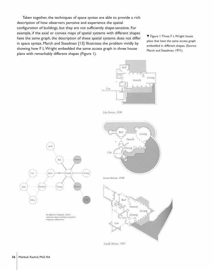
Taken together, the techniques of space syntax are able to provide a richdescription of how observers perceive and experience the spatialconfiguration of buildings, but they are not sufficiently shape-sensitive. Forexample, if the axial or convex maps of spatial systems with different shapeshave the same graph, the description of these spatial systems does not differin space syntax. March and Steadman [13] Illustrates the problem vividly byshowing how F L Wright embedded the same access graph in three houseplans with remarkably different shapes (Figure 1).

� Figure 1:Three F L Wright house

plans that have the same access graph

embedded in different shapes. (Source:

March and Steadman, 1971).

36 Mahbub Rashid, PhD, RA

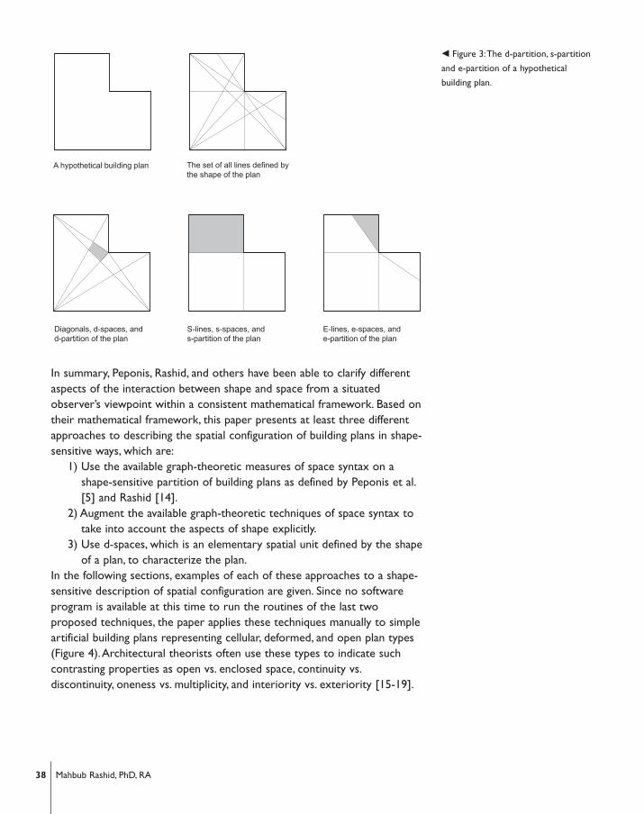
Hillier [10] applied graph theoretic measures to rectangular tessellationsembedded in different shapes in an attempt to overcome this problem.However, Hillier’s rectangular tessellations are not intrinsically related to theshapes they helped describe (Figure 2). In the late 1990s, Peponis, Rashid,and colleagues recognized this limitation of early space syntax moreexplicitly, and proposed shape-sensitive ways to describe visual experienceof a situated observer [5, 14]. Inspired by Hillier’s overlapping convexpartition, Peponis and colleagues [5] use walls of a plan and their surfaces togenerate a number of shape-sensitive partitions (Figure 3).They use wallsand s-lines (i.e., the extensions of extendible walls or surfaces) to define thes-partition with discrete s-spaces; and walls and e-lines (i.e., the extensionsof extendible walls and diagonals) to define the e-partition with discrete e-spaces.The s-partition of a plan is important, because each time an observercrosses an s-line an entire surface either appears into or disappears fromher visual field. In contrast, each e-line in an e-partition demarcates a changein the visibility of the endpoint/s of wall/s.They are also informationallystable because from any point within an e-space the number of visibleendpoints remains unchanged. In addition to s- and e-partitions, walls andsurfaces of a plan also help define the d-partition, which is composed of allthe d-spaces generated by the diagonals in a plan.This partition representsall possible triangulations of visibility between the endpoints of the plan[14].Triangulation is important because it represents the most elementarystructure of visual relations defined by the endpoints of a plan.

Peponis and his colleagues also help make the synthesis between formand space stronger by providing a process to determine the smallestnumber of positions on the e-partition of a plan from which all surfaces ofthe plan become visible [5].They argue that establishing such a set ofpositions is a step forward toward describing complicated shapes of buildingplans according to a more economical pattern. More recently, Rashid [15]provides techniques to characterize building plans based on mutual visibilityof the points defined by the walls and their surfaces within a plan.With thehelp of these techniques, Rashid is able to describe several elusiveproperties of different types of building plans.

� Figure 2:A shape may have different

degrees of spatial differentiation

depending on the size of the

tessellation used by Hillier (1996).


In summary, Peponis, Rashid, and others have been able to clarify differentaspects of the interaction between shape and space from a situatedobserver’s viewpoint within a consistent mathematical framework. Based ontheir mathematical framework, this paper presents at least three differentapproaches to describing the spatial configuration of building plans in shape-sensitive ways, which are:

1) Use the available graph-theoretic measures of space syntax on ashape-sensitive partition of building plans as defined by Peponis et al.[5] and Rashid [14].

2) Augment the available graph-theoretic techniques of space syntax totake into account the aspects of shape explicitly.

3) Use d-spaces, which is an elementary spatial unit defined by the shapeof a plan, to characterize the plan.

In the following sections, examples of each of these approaches to a shape-sensitive description of spatial configuration are given. Since no softwareprogram is available at this time to run the routines of the last twoproposed techniques, the paper applies these techniques manually to simpleartificial building plans representing cellular, deformed, and open plan types(Figure 4).Architectural theorists often use these types to indicate suchcontrasting properties as open vs. enclosed space, continuity vs.discontinuity, oneness vs. multiplicity, and interiority vs. exteriority [15-19].

� Figure 3:The d-partition, s-partition

and e-partition of a hypothetical

building plan.


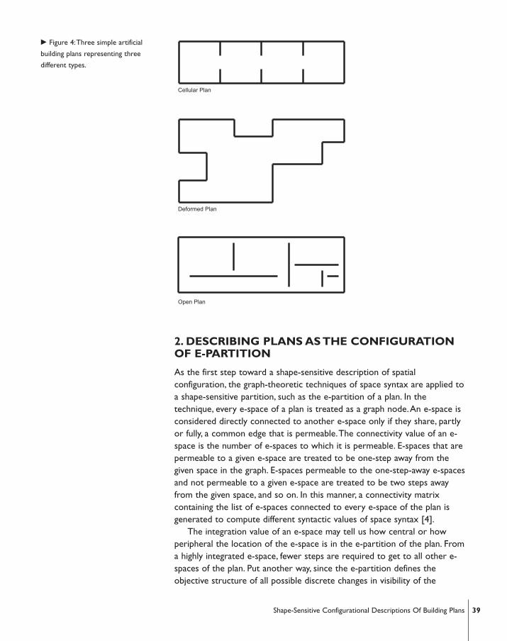
2. DESCRIBING PLANS AS THE CONFIGURATIONOF E-PARTITION

As the first step toward a shape-sensitive description of spatialconfiguration, the graph-theoretic techniques of space syntax are applied toa shape-sensitive partition, such as the e-partition of a plan. In thetechnique, every e-space of a plan is treated as a graph node.An e-space isconsidered directly connected to another e-space only if they share, partlyor fully, a common edge that is permeable.The connectivity value of an e-space is the number of e-spaces to which it is permeable. E-spaces that arepermeable to a given e-space are treated to be one-step away from thegiven space in the graph. E-spaces permeable to the one-step-away e-spacesand not permeable to a given e-space are treated to be two steps awayfrom the given space, and so on. In this manner, a connectivity matrixcontaining the list of e-spaces connected to every e-space of the plan isgenerated to compute different syntactic values of space syntax [4].

The integration value of an e-space may tell us how central or howperipheral the location of the e-space is in the e-partition of the plan. Froma highly integrated e-space, fewer steps are required to get to all other e-spaces of the plan. Put another way, since the e-partition defines theobjective structure of all possible discrete changes in visibility of the

� Figure 4:Three simple artificial

building plans representing three

different types.


vertices of a plan, it may be said that from a highly integrated e-space fewersteps are required to experience all possible discrete changes in visibility ofthe vertices of the plan. By implication, in a plan with high mean integrationthe average number of steps is fewer than that required in a plan with lowmean integration to experience all discrete changes in visibility of thevertices.To the extent changes in visibility of the vertices are a measure ofthe visual complexity of a plan, we may say that an integrated e-spaceprovides a less complex visual experience of the shape of the plan.

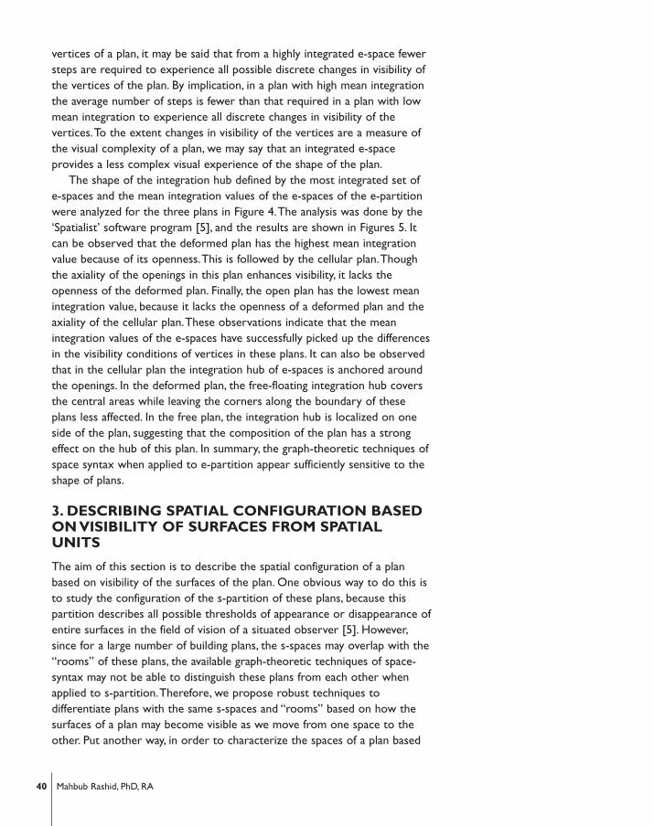
The shape of the integration hub defined by the most integrated set ofe-spaces and the mean integration values of the e-spaces of the e-partitionwere analyzed for the three plans in Figure 4.The analysis was done by the‘Spatialist’ software program [5], and the results are shown in Figures 5. Itcan be observed that the deformed plan has the highest mean integrationvalue because of its openness.This is followed by the cellular plan.Thoughthe axiality of the openings in this plan enhances visibility, it lacks theopenness of the deformed plan. Finally, the open plan has the lowest meanintegration value, because it lacks the openness of a deformed plan and theaxiality of the cellular plan.These observations indicate that the meanintegration values of the e-spaces have successfully picked up the differencesin the visibility conditions of vertices in these plans. It can also be observedthat in the cellular plan the integration hub of e-spaces is anchored aroundthe openings. In the deformed plan, the free-floating integration hub coversthe central areas while leaving the corners along the boundary of theseplans less affected. In the free plan, the integration hub is localized on oneside of the plan, suggesting that the composition of the plan has a strongeffect on the hub of this plan. In summary, the graph-theoretic techniques ofspace syntax when applied to e-partition appear sufficiently sensitive to theshape of plans.

3. DESCRIBING SPATIAL CONFIGURATION BASEDON VISIBILITY OF SURFACES FROM SPATIALUNITS

The aim of this section is to describe the spatial configuration of a planbased on visibility of the surfaces of the plan. One obvious way to do this isto study the configuration of the s-partition of these plans, because thispartition describes all possible thresholds of appearance or disappearance ofentire surfaces in the field of vision of a situated observer [5]. However,since for a large number of building plans, the s-spaces may overlap with the“rooms” of these plans, the available graph-theoretic techniques of space-syntax may not be able to distinguish these plans from each other whenapplied to s-partition.Therefore, we propose robust techniques todifferentiate plans with the same s-spaces and “rooms” based on how thesurfaces of a plan may become visible as we move from one space to theother. Put another way, in order to characterize the spaces of a plan based


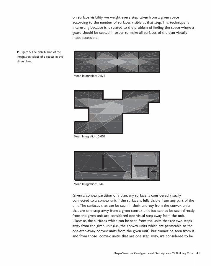
on surface visibility, we weight every step taken from a given spaceaccording to the number of surfaces visible at that step.This technique isinteresting because it is related to the problem of finding the space where aguard should be seated in order to make all surfaces of the plan visuallymost accessible.

Given a convex partition of a plan, any surface is considered visuallyconnected to a convex unit if the surface is fully visible from any part of theunit.The surfaces that can be seen in their entirety from the convex unitsthat are one-step away from a given convex unit but cannot be seen directlyfrom the given unit are considered one visual-step away from the unit.Likewise, the surfaces which can be seen from the units that are two stepsaway from the given unit (i.e., the convex units which are permeable to theone-step-away convex units from the given unit), but cannot be seen from itand from those convex unit/s that are one step away, are considered to be

� Figure 5:The distribution of the

integration values of e-spaces in the

three plans.


two visual steps away. In this manner, it is possible to determine how manysteps one has to take from a given convex unit in order to see all thesurfaces of a plan.We may call this the visual-depth of surfaces from thegiven convex unit. Note, however, that it may not be necessary to go toevery convex unit in a plan in order to see all the surfaces of the plan.

In order to calculate the “total visual depth of surfaces” from any givenunit within a plan, every surface, not every convex unit, is given a visualdepth value according to how many steps one needs to take from the givenunit in order to see the surface in its entirety.The sum of the values iscalled the total visual depth of surfaces from the given unit.The followingtable illustrates the procedure to compute the value taking Space #2 of theplan in Figure 6 as an example.

#Step #Spaces Reached #Surfaces visible Visual depth value

0 {2} {1,6,7,8,9,10,11,16,17} 0*9=0

1 {1,3} {2,3,4,5,12,13,14,15,21} 1*9=9

2 {4} {18,19,20,22} 2*4=8

Total visual depth of surfaces or TVDS from Space #2 17 � Figure 6: Procedure to compute the

surface visibility index taking space#2

as an example.


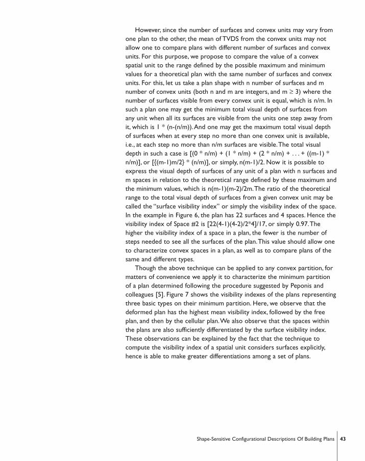
However, since the number of surfaces and convex units may vary fromone plan to the other, the mean of TVDS from the convex units may notallow one to compare plans with different number of surfaces and convexunits. For this purpose, we propose to compare the value of a convexspatial unit to the range defined by the possible maximum and minimumvalues for a theoretical plan with the same number of surfaces and convexunits. For this, let us take a plan shape with n number of surfaces and mnumber of convex units (both n and m are integers, and m ≥ 3) where thenumber of surfaces visible from every convex unit is equal, which is n/m. Insuch a plan one may get the minimum total visual depth of surfaces fromany unit when all its surfaces are visible from the units one step away fromit, which is 1 * (n-(n/m)).And one may get the maximum total visual depthof surfaces when at every step no more than one convex unit is available,i.e., at each step no more than n/m surfaces are visible.The total visualdepth in such a case is [(0 * n/m) + (1 * n/m) + (2 * n/m) + . . . + ((m-1) *n/m)], or [{(m-1)m/2} * (n/m)], or simply, n(m-1)/2. Now it is possible toexpress the visual depth of surfaces of any unit of a plan with n surfaces andm spaces in relation to the theoretical range defined by these maximum andthe minimum values, which is n(m-1)(m-2)/2m.The ratio of the theoreticalrange to the total visual depth of surfaces from a given convex unit may becalled the “surface visibility index” or simply the visibility index of the space.In the example in Figure 6, the plan has 22 surfaces and 4 spaces. Hence thevisibility index of Space #2 is [22(4-1)(4-2)/2*4]/17, or simply 0.97.Thehigher the visibility index of a space in a plan, the fewer is the number ofsteps needed to see all the surfaces of the plan.This value should allow oneto characterize convex spaces in a plan, as well as to compare plans of thesame and different types.

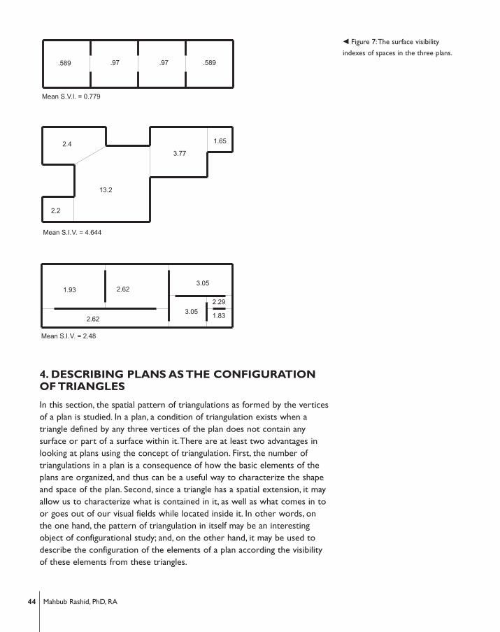
Though the above technique can be applied to any convex partition, formatters of convenience we apply it to characterize the minimum partitionof a plan determined following the procedure suggested by Peponis andcolleagues [5]. Figure 7 shows the visibility indexes of the plans representingthree basic types on their minimum partition. Here, we observe that thedeformed plan has the highest mean visibility index, followed by the freeplan, and then by the cellular plan.We also observe that the spaces withinthe plans are also sufficiently differentiated by the surface visibility index.These observations can be explained by the fact that the technique tocompute the visibility index of a spatial unit considers surfaces explicitly,hence is able to make greater differentiations among a set of plans.


4. DESCRIBING PLANS AS THE CONFIGURATIONOF TRIANGLES

In this section, the spatial pattern of triangulations as formed by the verticesof a plan is studied. In a plan, a condition of triangulation exists when atriangle defined by any three vertices of the plan does not contain anysurface or part of a surface within it.There are at least two advantages inlooking at plans using the concept of triangulation. First, the number oftriangulations in a plan is a consequence of how the basic elements of theplans are organized, and thus can be a useful way to characterize the shapeand space of the plan. Second, since a triangle has a spatial extension, it mayallow us to characterize what is contained in it, as well as what comes in toor goes out of our visual fields while located inside it. In other words, onthe one hand, the pattern of triangulation in itself may be an interestingobject of configurational study; and, on the other hand, it may be used todescribe the configuration of the elements of a plan according the visibilityof these elements from these triangles.

� Figure 7:The surface visibility

indexes of spaces in the three plans.


In discrete and, more recently, in computational geometry triangulationis used as an important partition of a geometric domain.According toToussaint, a set P, of n points in the plane, is triangulated by a subset,T, ofthe straight-line segments whose endpoints are in P, if T is a maximal subsetsuch that the line segments in T intersect only at their endpoints [20]. Insimple English, a point set is triangulated when its members are connectedby the maximum number of non-crossing diagonals or diagonals thatintersect at their endpoints only. Likewise, if we add as many non-crossingdiagonals as possible in a polygon or in a polyhedron we get thetriangulation of the polygon or of the polyhedra. More generally, then, atriangulation is a partition of a geometric domain, such as a point set,polygon, or polyhedron, into triangles that meet only at shared faces [21].

However, in contrast to the above definition where triangulation is usedas a partition, the paper treats triangulation as a cover, i.e., a collection oftriangles whose union is exactly the plan. Since triangulation is treated as acover, as opposed to a partition where triangles are not allowed tointersect except at their faces, there can be any number of triangles whichmay intersect or overlap each other, or which may contain one another.One of the primary reasons to use triangulation as a cover, rather than as apartition, is that the aim of the paper is to characterize plans based on therelational pattern of the triangles themselves. For its purpose, the papercharacterizes any given region within a plan based on the number of convextriangles each of which contains the given region.

4.1. Characterizing plans using triangulation

In a plan, wall surfaces restrict the visibility of its vertices. For plans with agiven number of surfaces and vertices, the number of visibility relations maydepend on the way surfaces are composed in these plans.As a result, thenumber of triangles may also vary in these plans. Naturally, for plans with ahigh visual density (i.e., with a higher number of diagonals between itsvertices) there may exist a high number of triangulations. Likewise, for planswith a poor visual density, there may exist a low number of diagonalsbetween its vertices, hence a low number of triangulations. Since thenumber of triangulations in a plan depends also on the number of itsvertices, the number of all possible convex triangles of a plan is divided bythe range defined by the maximum and minimum number of convextriangles possible for any plan with the same number of vertices in order tocharacterize and compare plans with different numbers of vertices.Thisratio is called the triangulation index of the plan. If one considers visualdensity as a measure of the visibility condition in a plan, then a hightriangulation index may suggest a better visibility condition in the plan.

In order to determine the triangulation index of a plan, first one needsto determine the number of convex triangles in the plan. For this, the


vertices of the plan are labeled from 1 to n.Any triangle that includesvertex1 is identified and listed:

{1,2,3}, {1,2,4}, {1,2,5} … {1,2,n}{1,3,4}, {1,3,5}, {1,3,6} … {1,3,n}{1,4,5}, {1,4,6}, {1,4,7} … {1,4,n}…{1,(n-2),(n-1)}, {1,(n-2),n}{1,(n-1),n}Once all possible triangles that include vertex1 are listed, the vertex is

dropped from the list of the vertices to be considered for furthertriangulation, and any triangle that includes vertex 2 is identified and listed.In a similar manner, when vertex 3 is considered, vertex1 and vertex 2 aredropped from the list of vertices to be considered for further triangulation.The process is continued until vertex (n-2) is reached, which has onetriangle, {(n-2),(n-1),n}, in its list.At this stage, all the non-convex trianglesare eliminated from the set of all listed triangles in order to determine thenumber of convex triangles in a plan.

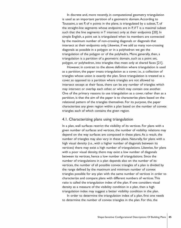
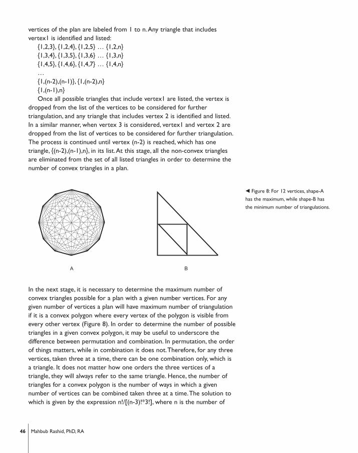
In the next stage, it is necessary to determine the maximum number ofconvex triangles possible for a plan with a given number vertices. For anygiven number of vertices a plan will have maximum number of triangulationif it is a convex polygon where every vertex of the polygon is visible fromevery other vertex (Figure 8). In order to determine the number of possibletriangles in a given convex polygon, it may be useful to underscore thedifference between permutation and combination. In permutation, the orderof things matters, while in combination it does not.Therefore, for any threevertices, taken three at a time, there can be one combination only, which isa triangle. It does not matter how one orders the three vertices of atriangle, they will always refer to the same triangle. Hence, the number oftriangles for a convex polygon is the number of ways in which a givennumber of vertices can be combined taken three at a time.The solution towhich is given by the expression n!/[(n-3)!*3!], where n is the number of

� Figure 8: For 12 vertices, shape-A

has the maximum, while shape-B has

the minimum number of triangulations.


vertices. For example, for a convex 10-gon the number of triangulationspossible between its vertices are 10!/[(10-3)!*3!], which is equal to 120.

In the following stage, it is necessary to determine the minimum numberof convex triangles possible for a plan with a given number of vertices. For agiven number of vertices a shape will have the least number of triangles, if itis possible to partition the plan is such a way that no more than threevertices of the plan are contained by a convex region (Figure 8).Theminimum number of possible triangles for an n-vertex plan is equal to n/3only when n is divisible by three. Note, however, that there are numbersthat are not divisible by three, hence cannot be partitioned in clusters ofthree. For such numbers it is also possible to define the minimum numberof triangulations.When n is not divisible by three, the remainder is either 1or 2.When the remainder is 1, the number of minimum triangles is equal to(n-4)/3 plus the minimum number of triangles for a 4-gon.And when theremainder is 2, the number of minimum triangles is (n-5)/3 plus theminimum number of triangles for a 5-gon.The minimum number of trianglefor a 4-vertex plan is two, and for a 5-vertex plan is three.Thus, for a 10-vertex plan the minimum number of triangle is [(10-4)/3]+2, which is 4.Andfor a 11-vertex plan it is [(11-5)/3]+3, which is 5. Once the number ofconvex triangles of a plan with a given number of vertices, and the possiblemaximum and minimum number of convex triangles for the plans with thesame number of vertices are determined, it is possible to compute thetriangulation index of the plan using the techniques suggested earlier.

The triangulation indexes of the three plans in Figure 4 were computed.It can be observed that the deformed plan is visually least restricted with atriangulation index of 0.141 suggesting a greater sense of global integrity byapproximating a condition where everything sees everything else as in thecase of a convex polygon.The free plan is visually most restricted with atriangulation index of 0.087. It allows neither the global nor the local visualintegrity because of such compositional rules as asymmetry and non-axiality.Finally, the cellular plan provides an in-between condition with atriangulation index of 0.127, because the composition of the plan limitstriangulations within local regions reducing the total number oftriangulations in the plan. However, it should be noted here that if thenumber of vertices is very high around a local convex region of a cellularplan, the number of triangulations in the region may increase significantlysuggesting local integrity. In a cellular plan, it is also possible to enhance theglobal integrity while maintaining local integrity by allowing triangulationsacross the convex regions or the “rooms” by compositional properties suchas axiality and centrality.


4.2. Characterizing regions within a plan using triangulation

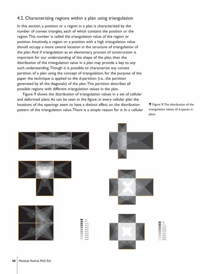
In this section, a position or a region in a plan is characterized by thenumber of convex triangles, each of which contains the position or theregion.This number is called the triangulation value of the region orposition. Intuitively, a region or a position with a high triangulation valueshould occupy a more central location in the structure of triangulation ofthe plan.And if triangulation as an elementary process of construction isimportant for our understanding of the shape of the plan, then thedistribution of the triangulation value in a plan may provide a key to anysuch understanding.Though it is possible to characterize any convexpartition of a plan using the concept of triangulation, for the purpose of thepaper the technique is applied to the d-partition (i.e., the partitiongenerated by all the diagonals) of the plan.This partition describes allpossible regions with different triangulation values in the plan.

Figure 9 shows the distribution of triangulation values in a set of cellularand deformed plans.As can be seen in the figure, in every cellular plan thelocations of the openings seem to have a distinct effect on the distributionpattern of the triangulation value.There is a simple reason for it: In a cellular


triangulation values of d-spaces in

plans.


plan, which is composed of rectangular units such as the ones in the figures,each unit would have only four triangulations amongst its own four verticeshad there been no opening. Openings introduce additional vertices to theseunits, and consequently the number of possible triangulations increaseswithin a local region. In fact, the more the number of vertices around aconvex unit, the more the number of triangulations within the unit. Inaddition, openings may also affect the distribution of the triangulation valueby providing further possibilities of triangulation across the convex units.Plans become globally oriented when openings allow triangulations acrossthese units, thus affecting our understanding of the plans as wholes.

The above suggestion is supported by the pattern of the distribution ofthe triangulation value in the deformed plans as well (Figure 9).The patternin each deformed plan suggests unambiguous centrality.This of course refersto the unity of the shape of these plans. However, the lack of any localcenter in these plans also suggests that in each of these cases the whole isachieved only at the cost of the parts. Nevertheless, the distribution patternalso picks up certain interesting differences between these plans. Forexample, in these deformed plans the changes made to the shape not onlyhave affected the triangulation values of d-spaces, but have also resulted indifferent forms of centrality.

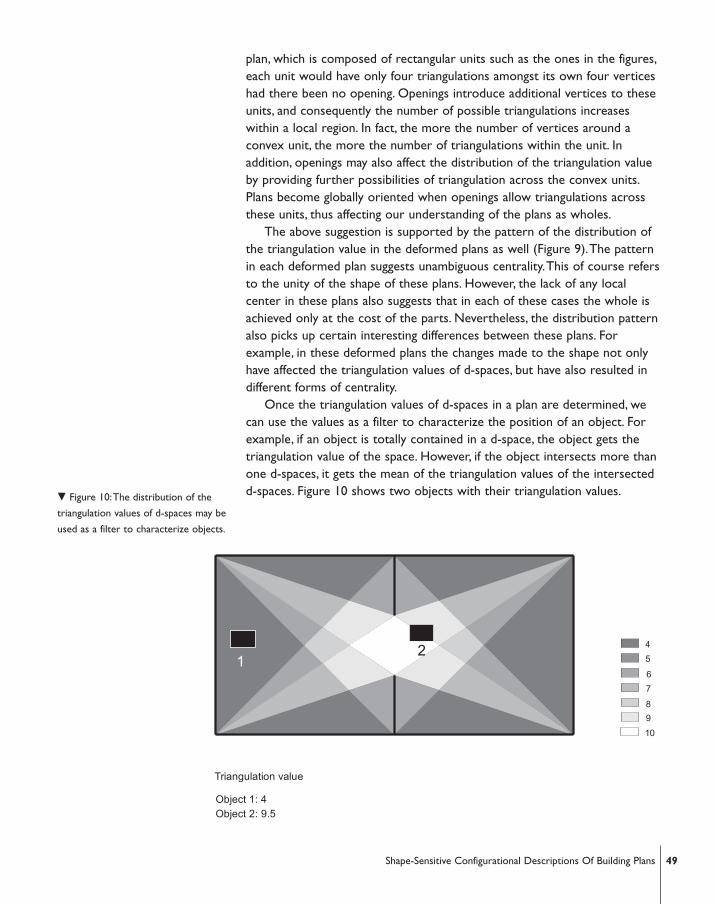
Once the triangulation values of d-spaces in a plan are determined, wecan use the values as a filter to characterize the position of an object. Forexample, if an object is totally contained in a d-space, the object gets thetriangulation value of the space. However, if the object intersects more thanone d-spaces, it gets the mean of the triangulation values of the intersectedd-spaces. Figure 10 shows two objects with their triangulation values.


triangulation values of d-spaces may be

used as a filter to characterize objects.


5. CONCLUSION

In this paper, techniques were developed to provide shape-sensitivedescriptions of the spatial configuration of buildings.To begin with, graph-theoretic techniques of space syntax were applied to the e-partition (i.e.,the most shape-sensitive partition of building plans) to characterize buildingplans.The mean integration values of the e-spaces and the shapes of theintegration hub of the e-spaces in these plans made it clear that thetechnique was sufficiently shape-sensitive.

Techniques were also developed to describe spatial configuration ofplans based on how surfaces become visible from spatial units. Here the keydescriptor was the surface visibility index.A space with a high visibility indexrequires fewer steps to see all the surfaces of the plan. Based on the study,it was possible to suggest that graph-theoretic techniques that considersurfaces explicitly were also able to provide shape-sensitive descriptions ofbuilding plans.

Finally, the concept of triangulation was used to describe theconfiguration of plans. Here the key descriptors were the triangulationindex and the triangulation value. It was suggested that higher triangulationindex of a plan should provide better visibility relations among the verticesof the plan, and that higher triangulation value of a spatial unit shouldindicate stronger centrality of a spatial unit in the structure of triangulationof the plan. Using these descriptors, interesting observations were made ona set of simple building plans. Since triangulation is a property intrinsic tothe shape of plans, any description of plans made using triangulation mayhelp bring the aspects of shape and space closer to each other inconfigurational studies than any other techniques suggested in this paper.

To conclude, we must note the relevance of the techniques proposedhere to visual perception in architecture.The literature indicates that ourvisual perception depends largely on the optic array, which is the pattern oflight provided to the eye by the environment and the objects containedwithin it, and that visual perception in architecture is often difficult todescribe for it must include both the static and dynamic optic arrays.Dynamic optic arrays—or the vista as J. J. Gibson calls it [22]—are neededto capture what and how the observer sees as she moves.They provide theinterface between the viewer and the world.

Earlier, Michael Benedikt [8] has proposed measures that quantify certainfeatures of isovists and isovist fields in a way that relates to the possibletransformations of a view in an architectural space. Over the last twodecades, space syntax has made isovists and isovist fields even morerelevant to architecture by providing techniques to study the relationalpatterns among an objectively defined set of isovists [e.g., 7, 12, 15]. In thefield of ecological optics, J. J. Gibson and his colleagues [23] made concertedefforts to analyze the information that is specific to the way surface are laidout in the three-dimensional space in which the viewer moves. Gibson’s


direct theory of perception holds that we respond directly to themathematic invariants in the transforming light to the eye.What is invariantdespite changes in viewpoint is of course the set of unchanging relationshipsamong the stationary surfaces in the environment. It is in this fact we mayfind the potential value of the techniques presented in this paper.Thesetechniques allow one to describe the unchanging relationships among alimited set of optic array that define the shape of the environment asrepresented in two-dimensional plans.With increasingly powerfulcomputers, there is no reason why these techniques cannot be extended todescribe the three-dimensional space or to describe more complicatedbuilding plans than the ones used in this study, thus enhancing ourunderstanding of the visual structure of the environment.

References1. Piaget, J., Psychology and Epistemology,Viking Press, New York, 1970.

2. Piaget, J., The Mechanisms of Perception, (Translated by G. N. Seagrim), BasicBooks, New York, 1969.

3. Piaget, J., and Inhelder, B., The Child’s Conception of Space, (Translated by F. J.Langdon, and J. L. Lunzer), Routledge & K. Paul, London, 1967.

4. Hillier, B., and Hanson, J., The Social Logic of Space, Cambridge, CambridgeUniversity Press, 1984.

5. Peponis, J.,Wineman, J., Rashid, M., Kim, S. H., Bafna, S., On the Description ofShape and Spatial Configuration Inside Buildings: Convex Partitions and TheirLocal Properties, Environment and Planning B: Planning and Design, 1997, 24, 761-781.

6. Peponis, J.,Wineman, J., Bafna, S., Rashid, M., Kim, S. H., On the Generation ofLinear Representations of Spatial Configuration, Environment and Planning B:Planning and Design, 1998, 25, 559-576.

7. Peponis, J.,Wineman, J., Rashid, M., Bafna, S., Kim, S. H., Describing PlanConfiguration According to the Co-visibility of Surfaces, Environment and PlanningB: Planning and Design, 1998, 25, 693-708.

8. Benedikt, M. L.,To Take Hold of Space: Isovists and Isovist Fields, Environment andPlanning B: Planning and Design, 1975, 6(1), 47-65.

9. Hanson, J., Deconstructing Architects’ Houses, Environment and Planning B:Planning and Design, 1994, 21, 675-704.

10. Hillier, B., Space is the Machine, Cambridge University Press, Cambridge, 1996.

11. Hillier, B., Specifically Architectural Knowledge, The Harvard Architecture Review,1993, 9, 8-27.

12. Turner,A., Doxa, M., O’Sullivan, D., Penn,A., From Isovists to Visibility Graphs:AMethodology For the Analysis of Architectural Space, Environment and Planning B:Planning and Design, 2001, 28, 103-121.

13. March, L., Steadman, P., The Geometry of Environment, MIT Press, Cambridge, MA,1971.

14. Rashid, M., On the Configurational Studies of Building Plans From the Viewpoint of aSituated Observer: A Partial Theory of Configuration For Plans Not Involving Curves,PhD Dissertation, Georgia Institute of Technology,Atlanta, Georgia, 1998.

15. Rashid, M., Mutual Visibility of Points in Building Plans, Journal of Architecture, 2011,16 (2), 231-266.


16. Giedion, S., Space,Time, and Architecture, Harvard University Press, Cambridge,MA, 1941, reprint 1967.

17. Zevi, B., Architecture As Space, Horizon Press, New York, 1957, reprint 1974.

18. Earl, F., and March, L.,Architectural Applications of Graph Theory, in:Wilson, R. B.,and Beineke, L.W. eds., Applications of Graph Theory,Academic Press, New York,1979.

19. Steadman, P., Built forms and Building Types: Some Speculations, Environment andPlanning B: Planning and Design, 1994, 21, 7-30.

20. Toussaint, G.T., Pattern Recognition and Geometrical Complexity, in: Proceedingsof the 5th International Conference on Pattern Recognition, Miami, FL, December 1-4,IEEE, New York, 1980, 1324-1347.

21. Bern, M.,Triangulations, in: Goodman J. E. and O’Rourke, J., eds., Handbook ofDiscrete and Computational Geometry, CRC Press, Boca Raton, 1997.

22. Gibson, J. J., The Senses Considered as Perceptual Systems, Houghton & Mifflin,Boston, 1966.

23. Gibson, J. J., The Ecological Approach to Visual Perception, Houghton & Mifflin,Boston, 1979.


Mahbub Rashid, PhD, RA

University of Kansas School of Architecture, Design, and Planning 1465 Jayhawk BoulevardLawrence, Kansas 66045

[email protected]

Documents

Shape-Sensitive Configurational Descriptions of Building Plans