Embed Size (px)
Citation preview
Non-parametric decoding on discrete time series and its applications inbioinformatics.
Hsieh Fushing, Univ. of California, Davis
Shu-Chun Chen, National Taiwan University,
Chii-Ruey Hwang, Math. Inst. Academia Sinica.
Short Title: Non-parametric decoding.
..............................................
Correspondence: Hsieh Fushing, Dept. of Statistics,
Mathematical Sciences Building, Univ. of California at Davis, CA 95616.
E-mail: [email protected]
1

Summary
We address the question: How do we non-parametrically decode the unknown state
space vector underlying a lengthy discrete time series possibly governed by one
non-autonomous dynamic with only two internal states? This question pertinently
reflects the dilemma of computing infeasibility against inferential bias found in many
scientific areas when considering whether to have, or not to have structural assump-
tions on the state space dynamics which are likely to be unrealistic. To resolve this
dilemma, the decoding problem is transformed into an event intensity change-point
problem without prior knowledge of the number of change-points involved. A new
decoding algorithm, called Hierarchical Factor Segmentation (HFS), is proposed to
achieve computability and robustness. Performance of the HFS algorithm in terms
of total decoding error is compared to the decoding benchmark Viterbi algorithm
through computer experiments. Under Hidden Markov Model (HMM) settings with
true parameter values, our HFS algorithm is competitive against the Viterbi algo-
rithm. Interestingly, when the Viterbi algorithm operates with maximum likelihood
estimated (MLE) parameter values, our HFS algorithm performs significantly bet-
ter. Similar favorable results are found when the Markov assumption is violated. We
further demonstrate one very important application of our HFS algorithm in bioin-
formatics as a promising computational solution for finding CpG islands – DNA
segments with aggregated CpG dinucleotides – on a genome sequence. A real illus-
tration on a subsequence of human chromosome #22 is carried out and compared
with one popular search algorithm.
Keywords: aggregating pattern; CpG island; Kullback distance; intensity change-
points analysis; maximum entropy distribution; Schwarz’ information criterion (BIC).
2

1 Introduction
Decoding is most often referred to in information theory as an algorithm for recov-
ering a sequence of code-words or messages, given a sequence of output signals in
communication through a noise channel (Geman and Kochanek, 2001). It is a task
corresponding to attempts to understand non-autonomous dynamics in mathemat-
ics and physics (Manuca and Savit, 1996). In general, a non-autonomous dynamic
is described via a system of difference, or differential, equations as:
∆X(t + 1) = G(X(t), S(t), θ);
∆S(t + 1) = F (S(t), ϑ). (1)
Here changes in an observable response variable X are regulated by the unobservable
internal state variable S(t) through G(· : θ), while S(t), also called the driving force,
is self-regulated by its own past history S(t) through F (· : ϑ). Thus the information
about the state space dynamics represented by F (· : ϑ) is the key to understanding
the whole dynamic.
In statistics, especially in time series literature, the idea of state-space models can
be traced back to a great extent to the non-autonomous dynamics given in equations
(1) above (Kalman, 1960; Durbin and Koopman, 2001; West and Harrison, 1997).
The functional forms of G(· : θ) and F (· : ϑ) are usually assumed known up to
the unknown parameters, as in mathematics, but the time series of Sn = {S(t) :
t = 1, 2, ..., n}, generally called the state space vector, is missing, as is often found
in physics. However, work on state space models commonly focuses on making
inferences about the parameters θ and ϑ under structural assumptions on G(·) and
F (·) based on the observed time series Xn = {X(t) : t = 1, 2, ..., n}. Most often,
if not always, the state space vector Sn is not the primary interest. It has become
routine that Sn is treated merely as missing data to be integrated out from the
complete data likelihood function of θ and ϑ in the EM-algorithm.
Here the specific task of recovering the unknown Sn based on Xn is called de-
3

coding. When G(· : θ) and F (· : ϑ) are assumed known up to θ and ϑ, this task is
called parametric decoding. Parametric decoding is popular in many real world ap-
plications, especially related to the Hidden Markov Model (HMM) with finite states.
For example, parametric decoding is used to compute the sequence of words given a
sequence of acoustic signals in speech recognition (Rabiner, 1989). It is also used to
compute the sequence of “business cycles,” or regime changes, given a time series of
the unemployment rate in quantitative finance and econometrics (Hamilton, 2005).
It is used to compute a sequence of exons and introns given a genome sequence in
computational genetics (Durbin, et al 1998). And as aforementioned, it is USED IN
computing a sequence of messages given an output signal sequence in information
theory (Geman and Kochanek, 2001).
From a computational perspective in parametric decoding, when the state vari-
able S(t) has a finite number |S| of states, decoding generally involves finding the
most “probable” n-vector of S(·) among |S|n possible configurations. An exhaustive
search for this most probable one is surely infeasible when n is large. Surprisingly,
under certain parametric structural assumptions, the decoding computation can be
reduced to a much more feasible level, such as one of order O(n|S|k) for a fixed num-
ber k. Usually this significant reduction in computation is achieved by a dynamic
programming technique. Thus most popular decoding algorithms have a dynamic
programming backbone. For example, the most widely used decoding technique is
the Viterbi algorithm (Viterbi, 1967). Its computation of the most likely configu-
ration can be achieved within O(n|S|2) operations (Geman and Kochanek, 2001).
Now several of its variant algorithms are also popular for different purposes, such
as the posterior Viterbi algorithm.
To put the achievements in parametric decoding in perspective, in order to
understand non-autonomous dynamics as a whole, it should be noted that these
parametric decoding algorithms all intrinsically rest on the parametric structural
assumptions. Therefore we can expect that these decoding results will be sensitive
4

to any assumption violation. In other words, parametric decoding can be rather
non-robust.
In this paper, decoding the unknown state space vector Sn, given no structural
assumptions imposed on the functionals G(·) and F (·), is our primary interest. This
task is termed “non-parametric decoding.” Thus the chief merits of non-parametric
decoding are freedom from the sensitivity of parametric assumptions, and avoidance
of biased statistical inference when extracting information of F (·).
Our non-parametric decoding algorithm is called the Hierarchical Factor Seg-
mentation (HFS) algorithm. It was originally developed in Fushing, et al. (2006)
for compressing the recording of animal behavior. In addition to the study of ani-
mal behavior, this technique has been shown to successfully provide very promising
results in the study of Circadian rhythms, psychological and emotional coherence,
and stock dynamics in several separate reports by the authors.
From the computational perspective under a nonparametric setting, there is no
platform for dynamic programming techniques, neither is an exhaustive search pos-
sible. Since the state variable S(t) only takes two values, ideally the non-parametric
decoding can be thought of as a task in change-point analysis, but without prior
knowledge as to how many change-point are involved. This is still a problem with
computing infeasibility.
To overcome this difficulty, the theoretical aspect of the HFS algorithm is briefly
depicted as follows. Instead of directly analyzing the measurement of Xn, we trans-
form this time series into a 0 or 1 record of a recurrent characteristic event. Our
HFS algorithm is performed on this 0-1 time series to partition the whole time se-
ries into segments, such that between adjacent segments intensities of the chosen
characteristic event are significantly different. Then a model selection problem in
deduced, and the Schwarz information criterion (BIC) is applied to select the “best”
partitions. The computational aspect of the HFS algorithm, as will be see in Section
3, is indeed very practical.
5

Regarding the decoding performance of the HFS algorithm, a series of computer
experiments are carried out, and the total number of decoding errors is used as the
performance index. Surprisingly, our HFS algorithm with its threshold parameters
selected via the Schwarz information criterion (BIC) achieves a very competitive
performance when compared to the benchmark Viterbi algorithm with the true
parameter values under the HMM setting. Very importantly, again under the same
HMM settings, the HFS algorithm is demonstrated to exhibit a performance much
superior to that of the Viterbi algorithm with maximum likelihood estimates (MLE)
for the parameter values. Furthermore, we also show that the performance of the
Viterbi algorithm is not as desirable as that of the HFS when the Markov structural
assumption is misspecified.
We then apply the HFS algorithm to identify CpG islands on a human genome
subsequence 1.4× 10⁵ base pairs long. We further demonstrate that our HFS algo-
rithm is a promising computational solution for finding CpG islands, which is one
very important issue in bioinformatics. The significance of finding CpG islands is
that this genome segment, with a high content of CpG dinucleotides (i.e., a cytosine
directly followed by a guanine), is found in most expressed genes (see Bird, 1986;
Bock, et al., 2007; Saxonov, et al., 2006). Recently its epigenome and functional
properties in normal and diseased cells or tissues have been under very intensive
investigation in biological and biomedical research. However, so far in bioinformat-
ics and computational genetics literature the identification of CpG islands is still
carried out through more or less ad hoc algorithms, or by the Viterbi algorithm and
its variants, where the Markov assumption is known to be invalid. Our HFS algo-
rithm provides very efficient computations for identifying CpG islands based on its
original epigenomic property. Indeed this is the problem that motivated our study.
This paper is organized as follows. The setting of a non-autonomous dynamic
system and computational measurements of evidence for an event aggregating pat-
tern is discussed in Section 2. Our HFS algorithm is introduced in Section 3 and
6

its optimal threshold values are derived in Section 4. In Section 5, we report the
results of computer experiments under HMM and beyond HMM settings. Real data
analysis of CpG islands is reported in Section 6. The final discussion section collects
several decoding-related issues.
2 Heuristic ideas, event aggregating patterns and
maximum entropy
In this section, we lay out the setting for decoding algorithms. To prepare the
development of the HFS algorithm, we discuss some related heuristic ideas, how
to perceive event aggregating patterns, and why the maximum entropy principle is
needed.
Throughout this paper we work on a discrete time series Xn of length n, with
X(t) taking values from a finite set of symbols A = {A1, ..., AK}, for t = 1, 2, ..., n.
Our development can easily be applied to time series of continuous measurement.
While the state variable S(t) takes only 0 or 1 values, X(t) is distributed according
to a discrete probability PS(t) defined on A = {A1, ..., AK}. Here we suppose that
for all symbols Ak ∈ A, 0 < P0(Ak)P1(Ak)
< ∞, so that no event can identify a state on
S(t) with certainty. As for the HMM setting, the Markov property of order one
is used for simplicity. This corresponds to a very simple linear graphic structure
sequentially linking S(1) through S(n). See Geman and Kochanek (2001) for an
example of a HMM represented by a more complex graph.
2.1 Heuristic ideas
The idea behind our development in this paper goes heuristically as follows: first,
we empirically choose an observable event that has the potential of separating P0
from P1; second, we then find evidence whether there exists an aggregating pattern
of such an event; third, the HFS algorithm is used to construct a segmentation on
Xn as a quasi-structure on Sn; fourth, by applying the maximum entropy principle
7

to each segment of the segmentation, a likelihood of two intensity parameters is
derived; and finally, the Schwarz information criterion is used to select the “best”
segmentation of Xn.
Therefore we do not construct a likelihood function for P0 and P1 and their
transition probabilities as in the HMM setting. Once a decoded Sn is available
from the HFS algorithm, statistical inference about P0 and P1 and the governing
dynamics of Sn become possible. Discussion of these related issues are deferred to
a separate study because they involve inferences that are rather distinct from the
decoding issues, which are the focus here, and would certainly lengthen this paper
considerably.
More specifically a segmentation of Xn can be perceived as a spatial mapping
for heterogeneity of recurrence times of the chosen event. In Subsection 2.2 we
try to evaluate the evidence of whether this particular event indeed reveals uneven
aggregating patterns on Xn. In Subsection 2.3, we look at an aspect of evidence
of aggregating patterns by comparing the empirical one to its maximum entropy
background, which supposedly contains no aggregating patterns at all.
2.2 Maximum entropy background
Consider a generic event of interest A taken from a σ-field constructed based on Ak
with small constant integer k(<< n). With event A, the observed time series Xn is
transformed into a 0-1 digital string, denoted by C0 = (C0(k), ...., C0(n − k + 1)),
according to the following coding scheme: C0(t) = 1 if event A is observed at time
t on Xn; otherwise, C0(t) = 0. A schematic coding on a genome subsequence and
an illustrative real example of C0 with k = 2 are given in Figs. 1(a) and (b),
respectively.
A permutation of C0 is denoted by C0σ = (C0(σ(1)), . . . , C0(σ(i)), . . . , C0(σ(n)))
with (σ(1), .., σ(i), . . . , σ(n)) being a permutation of (1, . . . , i, . . . , n). Further, we
use the notations TA, fA and c = E[TA] = E[TA|C0] to respectively denote the
recurrence time random variable, its frequency and the average recurrence time of
8

code word 1 on C0. These are equivalent to the recurrence time random variable
and frequency of event A along Xn.
It is noted that, given the event A, the frequency fA is invariant with respect to
all permutations on C0. We can show that the average recurrence time c = E[TA] is
nearly invariant in the sense that |c−E[TA|C0σ]| = Op(1/n). With the two invariance
properties, we can also perceive that the distribution of the recurrence time random
variable TA on the permuted digital string C0σ should be very close to the maximum
entropy distribution given the constraint c = E[TA]. As will be derived below, this
maximum entropy distribution turns out to be a geometric distribution GME(λ)
with characteristic intensity λ = log { cc−1} and fA = 1/c.
The maximum entropy distribution is derived as follows. Under the constraint
that the event A’s mean recurrence time E[T ] = c =∑∞
i=1 ipi is the only available
information pertaining to the non-autonomous dynamics of interest, the maximum
entropy distribution of TA is specified by:
p1 = 1/c;
pi = 1/ceλ(i−1);
λ = log{
c
c− 1
}
This geometric distribution is derived through the Lagrange Multiplier approach via
the target function
Q(p, λ) =∞∑i=0
pi log pi + η1
( ∞∑i=1
ipi − c
)+ η2
( ∞∑i=1
pi − 1
).
Thus from here on we take the geometric distribution GME(λ) as the background
distribution to be compared to the empirical one summarized from C0. An illustra-
tive comparison of the two distributions is given in Fig.1 (c) and (d). If there is
more invariant information available, than the same derivation would allow us to
compute the corresponding maximum entropy distribution.
9

2.3 Evidence of event aggregating patterns
We construct the empirical recurrence time distribution, or histogram, of TA from C0
and denote it as H∗. In order to perceive whether H∗ contains information about an
aggregating pattern of event A, we compare H∗ with the maximum entropy geomet-
ric distribution GME(λ) with λ = log { cc−1} and average recurrence time ˆE[TA] = c.
Heuristically, when there exist aggregating patterns along C0, H∗ should manifest
one vivid distinction from GME(λ): H∗ has higher probabilities on relatively ex-
tremely small as well as relatively extremely large recurrence times than that of
GME(λ), while the pattern is reversed on the middle region of recurrence time. This
distinct feature is illustrated in Fig. 1 based on a genome subsequence from human
chromosome #22. Visually, Fig. 1(b) shows a rather clear alternating pattern of
aggregation and sparsity of CG dinucleotides. These visual patterns are reflected in
the aforementioned distinction between GME(λ) and RA as shown in panel (c), and
even more vividly in panel (d).
10

Location 1 2 3 4 5 ……..………...13…....16…………………..........................32……G G G C G G A A A G A T C G C C G T G T A A T T C T A G A G T C G……
chormosome 22 bA111E21
Location
Se
gm
en
ts
0 2000 4000 6000 8000 10000
18
16
14
12
10
86
42
||| | || |||| | | | | | |||||||||||| |||| | |||||| || | || | | || | | ||| | | | | | | | || |||||||||||||| | || ||||||||||||||||| | |
| || || | | ||||||||||||||||||||||||||||||||||||||||||||||||||||||||||||||||||| |||||||||| |||||| | |||| | || ||||||||||||| ||| | | ||| | | || | | || || || | || | |||| ||||| | ||||| | || |
|||||||||||||||||| | ||||||| | | | | || || | || || || || ||||||||||||||||||||||||||||||||||||||||||||||||||||||||||||||||||||||||||||||||||||| | || | | | || | |||| | | | | ||| ||| || || |||| || || || | ||
|||| ||| | | | || | ||||||||||||||||||| || | | | ||| |||||||| | || | ||||| | | | | | | || | | | | | || | | | | ||||| ||||||
||| | | | || | || || || || | || | | |||||| | | || | | | | | | ||||||| ||| ||| |||||||||||||||||||||||||||||||||||| || || | | |||||
||||||||| | | | || | | | | || | || || | | || | || | | || | | | | | || | | | | |
|| ||||| | | | || | | | || | | || | || | ||| | | || ||||||| | | || ||||| |||| || |||||| ||| | ||||||||| | | |||| || || |
|||| ||| || || ||| | | | ||||| || | || | | | || | | | | | | | || ||| ||| ||| | | |||| | |||| ||| ||||| || ||| | | | |
| | |||| | || ||||||| || |||| | | | | | || | | || | | | ||| | | |||||||||||||||||||||||||||||||||||||||||||||||||||||||||||||||||||||||||||||||||||||||||||||| || | ||||||||||| ||| | ||| | |||
| | | | | | | || | || || || || | | | || | || | | || || | | | || | ||||||| ||| | | | | ||||| | |||| ||||| | ||||||||||||| | || | | ||||| ||| ||
|||| | ||| ||| || ||| || | || |||||| |||| ||||| | || | ||||||| | | | ||| |||||||| | | | |||||||||| | | | || | | | || | || | || |||| ||||| |||||||||||||||| |
||||||||| ||||||||| |||| |||| |||| ||||||||||| ||||||||||||||||| |||||||||||||||| ||||||||||||||||||||||||||||||||||||||||||||||||||||||||||| ||| || | |||||||||||||||| ||||||||||| |||||||||| ||||||| | ||| || || ||||||||| |||| |||||||||||||||||||| | ||||||||||||||||||||||||||||| |||||||||||||||||| ||||||| | | |
||||||||||||||||||||||||||||||||||||||||||| ||||||||||||||||||||||||||||||||||||||||||||||||||||||||||||||||||||||||||||||||||||||||||||||||||||||||||||||||||||||||||||||||||||||||||||||||||||||||||||||||||||||||||||||||||||||||||||||||||||||||||||||||||||||||||||||||||||||||||||||||||||||||||||||||||||||||||||||||||||||||||||||||||||||||||||||||||||||||||||||||||||||||||||||||||||||||||||||||||||||||||||||||||||||||||||||||||||||||||||||||||||||||||||||||||||||||||||||||||||||||||||||||||||||||||||||||||||||||||||||||||||||||||||||||||||||||||||||||||||||||||||||||||||||||||||||||||||||||||||||||||||||||||||||||||||||||||||||||||||||||||||||||||||||||||||||||||||||||||||||||||||||||||||||||||||||||||||||||||||||||||||||||||||||||||||||||||||||||||||||||||||||||||||||||||||||||||||||||||||||||||||||||||||||||| |||||||||||||||||||||||||||||||||||||||||||||||||||||||||||||||||||||||||||||||||||||||||||||||||||||||||||||||||||||||||||||||||||||||||||||||||||||||||||||||||||||||||||||||||||||||||||||||||||||||||||||||||||||||||||||||||||||||||||||||||||||||||||||||||||||||||||||||||||||||||||||||||||||||||||||||||||||||||||||||||||||||||||||||||||||||||||||||||||||||||||||||||||||||||||||||||||||||||||||||||||||||||||||||||||||||||||||||||||||||||||||||||||||||||||||||||||||||||||||||||||||||||||||||||||||||||||||||||||||||||||||||||||||||||||||
||||||||||||||||||||||||||||||||||||||||||||||||||||||||||||||||||||||||||||||||||||||||||||||||||||||||||||||||||||||||||||||||||||||||||||||||||||||||||||||||||||||||||||||||||||||||||||||||||||||||||||||||||||||||||||||||||||||||||||||||||||||||||||||||||||||||||||||||||||||||||||||||||||||||||||||||||||||||||||||||||||||||||||||||||||||||||||||||||||||||||||||||||||||||||||||||||||||||||||||||||||||||||||||||||||||||||||||||||||||||||||||||||||||||||||||||||||||||||||||||||||||||||||||||||||||||||||||||||||||||||||||||||||||||||||||||||||||||||||||||||||||||||||||||||||||||||||||||||||||||||||||||||||||||||||||||||||||||||||||||||||||||||||||||||||||||||||||||||||||||||||||||||||||||||||||||||||||||||||||||||||||||||||||||||||||||||||||||||||||||||||||||||||||||||||||||||||||||||||||||||||||||||||||||||||||||| |||||||||||| |||||||||||||||||||||||||||||||||||||||||||||||||||||||||| |||||||| |||||||||||||||||||||||||||||||||||||||||||||||||||||||||| |||||||| |||||||||||||||||||||||||||||||||||||||||||||||||||||||||| ||||||||||||||||||||||||||||||||| ||||||||||||||||||| |||||||||||
||||||||||||||||||||||||||| | ||||||||||||||||||||||||||||||||||||||||||||||||||||||||||||||||||||||||||||||||||||||||||||||||||||||||||||| ||||||||||||||||||||||||||||||||||||||||||||||||||||||| ||||||||||||||||||||||||||||||||||||||||||| |||||||||||||||||||||||||||||||||||||||||||||||| | | | || || || ||| | | | | ||||||||||||||||||||||||||||||||||||| ||||||||||||||||||||||||||||| |||||||||||||||||||| | | |
| | | | | || |||||||||||||||||||||||||||||||||||||||||||||||||||||||||||||||||||||||||||||||||||||||||||||||||||||||||||| | | | | ||||||| |||||||||| ||||||||||||||||||||||||||||||||||||||||||||||||| ||||||||| | |||||||||| | ||||||||||||||||||||||||| ||| |||||||||||||||||||||||||||||||| ||||||||||||||||| ||||||||| ||||||||||||||||
|||||||||||||||||||||||||||||||||||||||||||| | ||||||||||||||||| ||||||||||||||||||| |||||||||||||||||||||||||||||||||||||||||||||||| |||||||||||||||||||||||||| |||||||||||||||||| |||||||||||||||||| |||||||||||||||||| |||| | | |||||||||||||||||||||||||||||||||||||||||||| |||||| ||||||||||||||||||||||||||||||||||||||||||||||||||||||||||||||||||||||||||||||||||||||||||||||||||||||||||||||||||||||||||||||||||||||||||||||||||||||||||||||||||||||||||||||||||||||||||||||||||||||||||||||||||||||||||||||||||||||||||||||||||||||||||||||||||||||||||||||||||||||||||||||||||||||||||||||||||||||||||||||||||||||||||||||||||||||||||||||||||||||||||||||||||||||||||||||||||||||||||||||||||||||||||||||||||||||||||||||||||||||||||||||||||||||||||||||||||||||||||||||||||||||||||||||||||||||||||||||||||||||||||||||||||||||||||||||||||||||||||||||||||||||
|||||||||||||||||||||||||||||||||||||||||||||||||||||||||||||||||||||||||||||||||||||||||||||||||||||||||||||||||||||||||||||||||||||||||||||||||||||||||||||||||||||||||||||||||||||||||||||||||||||||||||||||||||||||||||||||||||||||||||||||||||||||||||||||||||||||||||||||||||||||||||||||||||||||||||||||||||||||||||||||||||||||||||||||||||||||||||||||||||||||||||||||||||||||||||||||||||||||||||||||||||||||||||||||||||||||||||||||||||||||||||||||||||||||||||||||||||||||||||||||||||||||||||||||||||||||||||||||||||||||||||||||||||||||||||||||||||||||||||||||||||||||||||||||||||||||||||||||||||||||||||||||||||||||||||||||||||||||||||||||||||||||||||||||||||||||||||||||||||||||||||||||||||||||||||||||||||||||||||||||||||||||||||||||||||||||||||||||||||||||||||||||||||||||||||||||||||||||||||||||||||||||||||||||||||||||||||||||||||||||||||||||||||||||||||||||||||||||||||||||||||||||||||||||||||||||||||||||||||||||||||||||||||||||||||||||||||||||||||||||||||||||||||||||||||||||||||||||||||||||||||||||||||||||||||||||||||||||||||||||||||||||||||||||||||||||||||||||||||||||||||||||||||||||||||||||||||||||||||||||||||||||||||||||||||||||||||||||||||||||||||||||||||||||||||||||||||||||||||||||||||||||||||||||||||||||||||||||||||||||||||||||||||||||||||||||||||||||||||||||||||||||||||||||||||||||||||||||||||||||||||||||||||||||||||||||||||||
(b)
(a)
recurrence time
Pro
ba
bility
0 500 1000 1500
0.0
00
.02
0.0
40
.06
0.0
80
.10
0.1
2
0.0 0.5 1.0 1.5 2.0 2.5 3.0
-3.5
-3.0
-2.5
-2.0
-1.5
-1.0
distance(log-scale,base=10)
Pro
bab
ility(l
og
-scale
,ba
se
=1
0)
(c) (d)
Fig.1 Event and event-time series, recurrencetime histogram and the maximum entropy dis-tribution. (a) The CG (one C followed by G)asthe chosen event, and a schematic transforma-tion of genome subsequence into an event-timeseries; (b) the event-time series; (c) the his-togram of recurrence time (H∗) and its cor-responding maximum entropy geometric distri-bution (GME(λ)); (d) H∗ vs GME(λ) on log-probability and log-time scale.
Though Fig. 1 reveals pictorial evidence of aggregating patterns, how to effec-
tively summarize such evidence quantitatively may not be obvious. For instance,
consider the Kullback distance between GME(λ) and H∗ defined as
K(H∗, GME(λ)) =∞∑i=1
H∗(i) logH∗(i)
GME(i : λ).
From Fig. 1(d), the log-probability ratios log H∗(i)
GME(i:λ)are positive for the two tail
regions, but negative on the middle region. Although the three regions are all
coherent with the aggregating pattern, the positive and negative cancelation would
make the Kullback distance a less effective summarizing statistic for evaluating the
11

characteristic feature. In order to resolve this shortcoming of Kullback distance, one
must determine how to mark the three regions first before evaluating a proposed
summarizing statistic. This task could involve smoothing techniques and possibly
some ad hoc choices of thresholds. Hence it is not at all a simple task that can be
done without potential disagreement.
In the next section, from the segmentation perspective, instead of comparing
GME(λ) and H∗, we propose a more effective methodology for evaluating an aggre-
gating pattern on Xn. Thus we are free from the above difficulty.
3 Hierarchical factor segmentation (HFS) algo-
rithm
The Hierarchical Factor Segmentation (HFS) algorithm is constructed based on the
event recurrent time distribution and multi-level coding schemes in this section.
Functionally it is designed to find where the aggregating patterns begin and end
along the temporal span of the time series of interest. Consequently the time series
is partitioned into alternating sequences of high and low event-intensity segments.
[Hierarchical factor segmentation(HFS) algorithm:] With a chosen ob-
servable event A on the time series Xn, the construction procedure of the HFS
algorithm is depicted via the following steps:
[HFS-1. ] By the event definition, Xn is transformed into 0-1 digital string of base 2
via the following coding scheme: code 1 for X(t) when the event is observed at
time t, otherwise code 0 for X(t). This first level 0-1 digital string is denoted
by the code sequence C0.
[HFS-2. ] Construct a histogram, says H∗, of the event recurrent time distribution
from C0, and denote the sequence of recurrence time (inter-event-spacing) by
R∗.
[HFS-3. ] Choose the first threshold value as an upper p∗ percentile on H∗, says
12

Cs, to transform the R∗ sequence into a 0∗-1∗ digital string via the second
level coding scheme: 1) a recurrent time less than Cs is coded by a 0∗; 2) a
recurrent time greater than Cs is coded by a 1∗. The resultant digital string
of base 2 is denoted by the code sequence C∗.
[HFS-4. ] Upon code sequence C∗, we take code word 1∗ as another “new” event
and construct its corresponding recurrent time histogramH@ and the sequence
of inter-1∗-event-spacing as R@.
[HFS-5. ] Choose the second threshold value as an upper p@ percentile from H@,
say Cs∗, to transform R@ into another 0@-1@ digital string via the top level
coding scheme: 1) an inter-1∗-event-spacing less than Cs∗ is coded by 0@; 2)
an inter-1∗-event-spacing greater than Cs∗ is coded by a 1@. The third digital
string of base 2 is denoted by C@.
HFS-6. The resultant code sequence C@ is mapped back on the time series C0 or
Xn as a partition of |R@|(= m) segments on the time span [1, n]. Denote this
partition as N (Xn) = {[NLi, NRi)}mi=1.
This partition or segmentation N (Xn) will be seen to achieve an aggregating pat-
tern by separating the high event-intensity segments against the low-event-intensity
ones. A segment, say [NLi, NRi), corresponding to 1@-code, is a period of time points
falling in between two widely separated 1∗-codes. The wide separation of two succes-
sive 1∗-codes implies that there are many 1-codes on the particular segment of code
sequence C0, equivalently, many events are observed on the segment of Xn. Thus
this is a segment of high event-intensity. In contrast, a segment, say [NLi′ , NRi′),
corresponding to 0@-code (including segments corresponding to the two 1∗-codes on
both of its ends) would present an extended period of having many 0-codes, but
very sparse 1-codes. Thus it is a segment of low event-intensity.
The computational essence of the HFS algorithm is that, under no parametric
assumptions, the number of partition N (Xn) pertaining to all the possible integer
13

threshold values (Cs,Cs∗) with regard to a chosen event is much less than 2n. It
is this small set of candidate partitions on Xn that will facilitate the computing
feasibility for model selection techniques, as discussed in the next section.
4 Intensity change-point analysis and Schwartz
information criterion (BIC)
After application of the HFS algorithm with threshold parameters (Cs,Cs∗), Xn
is partitioned into two classes of segments corresponding to code words 0@ and 1@
defining the segmentation N (Xn). Furthermore, we consider that the recurrence
time of event A within all segments corresponding to codeword 0@ is stationary and
geometrically distributed as G(· : λ0). In contrast, the recurrence time within all 1@
segments is stationary and G(· : λ1) distributed. Therefore any transition between
0@ and 1@ segments is taken as an intensity change-point. Denote the number of
change-points by H0(τ) with τ = (Cs,Cs∗) for notational simplicity.
Let {k0j}m0j=1 and {k1j′}m1
j′=1 denote the observed recurrent time in the 0@ and 1@
segments respectively. Next we compute the likelihood function of (λ0, λ1) based on
the observed recurrence times within the two classes of segments, assuming they are
independent copies, as
L(λ0, λ1) = Pm00 (λ0)
∏e−λ0(k0j−1)Pm1
0 (λ1)∏
e−λ1(k1j′−1) (2)
where P0(λ) = (1− e−λ), and m0 and m1 are the total number of recurrence times
on 0@ segments and 1@ segments, respectively.
The maximum likelihood estimates of (λ0, λ1) are derived as follows:
λ0 = log{
c0
c0 − 1
}λ1 = log
{c1
c1 − 1
}
where c0 =∑
k0j
m0and c1 =
∑k1j′
m1are the average recurrence times on 0@ segments
and 1@ segments, respectively.
14

As in the null case when no segmentation is imposed on Xn with the maximum
entropy applicable on its whole time span, the event recurrence time distribution is
again geometrically distributed. Indeed its maximum likelihood estimate coincides
with the maximum entropy distribution. This is due to the fact that the number of
events on Xn is a fixed constant. Denote this geometric distribution G(· : λ) with
λ = log 1+cc
, c = n/m and m = m0 + m1. The maximum likelihood affiliated with
G(· : λ) is calculated as L(λ|σ) = Pm0 (λ)e−λ(n−m).
Thus the log-likelihood ratio is computed as
∆0(τ) = log L(λ0, λ1|σ)− log L(λ|σ)
=1∑
k=0
[mk log
{1
ck − 1
}− lk log
{ck
ck − 1
}]
−[m log
{1
c− 1
}− n log
{c
c− 1
}]
where l0 + l1 = n, and l0 =∑
k0j and l1 =∑
k1j′ are the total lengths of the 0@ and
1@ segments, respectively.
It is clear that ∆0(τ) can be a reasonable and effective candidate for a test
statistic of the hypothesis of whether there exist aggregating patterns within Xn, as
briefly discussed in the previous section. It is worth emphasizing again here that
the number of change-points of event-intensity is unknown. Hence the lack of this
prior information raises an important question: Is ∆0(τ) approximately chi-squared
distributed, and, if so, with how many degrees of freedom under the null and the
alternative hypotheses? This question and the related regime change issues will be
addressed in detail in a separate report. Here we focus on the decoding issue.
To make use of ∆0(τ) for selecting an optimal threshold parameter τ in the
HFS algorithm, we apply the Schwartz’ information criterion, also called the BIC
criterion. That is, we perform the following optimization:
Γ(τ) = ∆0(τ)− log m
2(H0(τ) + 1)
τ opt = arg maxτ
[Γ(τ)]
15

¿From here on, the HFS algorithm is meant to be performed according the choice
of optimal threshold parameter τ opt.
Another closely-related alternative model selection procedure is based on the
minimum description length (MDL) of Rissanen (1996, 1997) (see also Lanterman
(2001) and Lee (2001) for review and tutorial). The MDL criterion applied in our
setting is the following:
Γ∗(τ) = ∆0(τ)− log n(H0(τ) + 1)− 1
2[log l0 + log l1]
τ opt∗ = arg maxτ
[Γ∗(τ)]
Based on experience from our computer experiments, the penalty for increasing the
number of change-points is too high. In fact, it might not be surprising, since this
criterion was derived when the order of the set of candidate partitions is 2n. In sharp
contrast, our set of candidate partitions via HFS is indeed many orders smaller.
5 Computer experiments under Hidden Markov
models and beyond
In this section we conduct computer experiments to numerically evaluate the decod-
ing performance of our HFS algorithm with the BIC-selected threshold parameter
τ opt. The performance index is measured through the average decoding error rate.
In the experiments, we also compute fully parametric decoding procedures via the
Viterbi and posterior-Viterbi algorithms under Hidden Markov Models (HMM) and
non-HMM models with the parameter values being either completely known or esti-
mated via the maximum likelihood estimation (MLE) approach. Their performances
are meant to serve as benchmarks for the decoding efficiency of the HFS algorithm.
5.1 HMM setting
Here we make use of the Hidden Markov Model setting with two dice: one is fair;
the other is loaded, an example considered in Durbin, et al. (1998, Chapter 3).
16

The alphabet is A = {1, 2, . . . , 6}, and the state P0(i) = 1/6 for the fair die is
designated as the state S(t) = 0, while the state P1(i) = 1/10 for i = 1, 2, . . . , 5,
and P1(6) = 1/2 for the loaded die is designated as the state S(t) = 1. The Markov
dynamic governed by the transition probability matrices of the two states 0 and 1 is
specified by p01 = Pr[S(t + 1) = 1 | S(t) = 0] and p10 = Pr[S(t + 1) = 0 | S(t) = 1].
Three cases of (p01, p10)s are considered: I)(p(1)01 , p
(1)10 ) = (0.05, 0.1); II) (p
(2)01 , p
(2)10 ) =
(0.1, 0.2); III) (p(3)01 , p
(3)10 ) = (0.4, 0.5).
The MLEs for all involved parameters are computed via the Baum-Welch algo-
rithm (Baum, 1970), which is equivalent to the EM algorithm (Dempster, Laird and
Rubin, 1977). The Viterbi algorithm, available in R-code, computes the most likely
configuration as:
SVn = arg max Pr[Sn | Xn,P1,P0, p10, p01]
with either the true parameter values of P1,P0, p10, p01 or their MLE estimates.
In contrast, the posterior-Viterbi algorithm computes the most likely S(t) for
each t individually as:
SPV (t) = arg max Pr[S(t) | Xn,P1,P0, p10, p01], t = 1, ...., n
also with either the true parameter values of P1,P0, p10, p01 or their MLE estimates.
In case I the state-space vector Sn is expected to have 11 . . . 11 segments (each
of expected length 10) being well-separated by 000 . . . 00 segments (each of expected
length 20). This kind of aggregating pattern in Sn is slightly blurred in case II due
to larger values of (p01, p10) and shorter expected lengths of repeating states. In case
III, it is very difficult to decode Sn, since the aggregating pattern almost disappears
into a fashion very close to that of a random fair coin toss.
As an illustration of our computational decoding results, the Occasionally Dis-
honest Casino example of Chapter 3 in Durbin, et al. (1998), is reanalyzed and
reported in Fig. 2. Based on the same data, the concave shape of Γ functions in
the BIC procedure over a region of threshold values is reported in Fig. 3. It is very
interestingly demonstrated as well that the modes of the concave curves are shown
17

to correspond to very low error rates, which is comparable to the benchmarks set by
the Viterbi and posterior-Viterbi algorithms with true parameter values. This corre-
sponding relationship indicates that the HFS algorithm with BIC-selected threshold
parameters captures the aggregating pattern on Sn fairly well in this data set. In
fact this case turns out to be rather typical under the Case I setting, as indicated
by results from a simulation study reported in Fig. 4.
3 1 5 1 1 6 2 4 6 4 4 6 6 4 4 2 4 5 3 1 1 3 2 1 6 3 1 1 6 4 1 5 2 1 3 3 6 2 5 1 4 4 5 4 3 6 3 1 6 51 1 1 1 1 1 1 1 1 1 1 1 1 1 1 1 1 1 1 1 1 1 1 1 1 1 1 1 1 1 1 1 1 1 1 1 1 1 1 1 1 1 1 1 1 0 0 0 0 01 1 1 1 1 1 1 1 1 1 1 1 1 1 1 1 1 1 1 1 1 1 1 1 1 1 1 1 1 1 1 1 1 1 1 1 1 1 1 1 1 1 1 1 1 1 1 1 0 01 1 1 1 1 1 1 1 1 1 1 1 1 1 1 1 1 1 1 1 1 1 1 1 1 1 1 1 1 1 1 1 1 1 1 1 1 1 1 1 1 1 1 1 1 1 1 0 0 01 1 1 1 1 1 1 1 1 1 1 1 1 1 1 1 1 1 1 1 1 1 1 1 1 1 1 1 1 1 1 1 1 1 1 1 1 1 1 1 1 1 1 1 1 0 0 0 0 0
RollsDieViterbiPost-VHFS
6 6 2 6 5 6 6 6 6 6 6 5 1 1 6 6 4 5 3 1 3 2 6 5 1 2 4 5 6 3 6 6 6 4 6 3 1 6 3 6 6 6 3 1 6 2 3 2 6 40 0 0 0 0 0 0 0 0 0 0 0 0 0 0 0 1 1 1 1 1 1 1 1 1 1 1 1 0 0 0 0 0 0 0 0 0 0 0 0 0 0 0 0 1 1 1 0 0 00 0 0 0 0 0 0 0 0 0 0 0 0 0 0 0 1 1 1 1 1 1 1 1 1 1 1 1 0 0 0 0 0 0 0 0 0 0 0 0 0 0 0 0 0 0 0 0 0 00 0 0 0 0 0 0 0 0 0 0 0 0 0 0 0 1 1 1 1 1 1 1 1 1 1 1 1 0 0 0 0 0 0 0 0 0 0 0 0 0 0 0 0 0 1 1 1 1 10 0 0 0 0 0 0 0 0 0 0 0 0 0 0 0 1 1 1 1 1 1 1 1 1 1 1 1 0 0 0 0 0 0 0 0 0 0 0 0 0 0 0 0 0 0 0 0 0 1
RollsDieViterbiPost-VHFS
5 5 2 3 6 2 6 6 6 6 6 6 2 5 1 5 1 6 3 1 2 2 2 5 5 5 4 4 1 6 6 6 5 6 6 5 6 3 5 6 4 3 2 4 3 6 4 1 3 10 0 0 0 0 0 0 0 0 0 0 1 1 1 1 1 1 1 1 1 1 1 1 1 1 1 1 1 0 0 0 0 0 0 0 0 0 0 0 0 0 1 1 1 1 1 1 1 1 10 0 0 0 0 0 0 0 0 0 0 0 1 1 1 1 1 1 1 1 1 1 1 1 1 1 1 1 1 1 1 1 1 1 1 1 1 1 1 1 1 1 1 1 1 1 1 1 1 11 1 1 1 0 0 0 0 0 0 0 0 1 1 1 1 1 1 1 1 1 1 1 1 1 1 1 1 1 0 0 0 0 0 0 0 0 0 1 1 1 1 1 1 1 1 1 1 1 11 1 1 1 0 0 0 0 0 0 0 0 1 1 1 1 1 1 1 1 1 1 1 1 1 1 1 1 1 0 0 0 0 0 0 0 0 0 0 0 1 1 1 1 1 1 1 1 1 1
RollsDieViterbiPost-VHFS
5 1 3 4 6 5 1 4 6 3 5 3 4 1 1 1 2 6 4 1 4 6 2 6 2 5 3 3 5 6 3 6 6 1 6 3 6 6 6 4 6 6 2 3 2 5 3 4 4 11 1 1 1 1 1 1 1 1 1 1 1 1 1 1 1 1 1 1 1 1 1 1 1 1 1 1 1 0 0 0 0 0 0 0 0 0 0 1 1 1 1 1 1 1 1 1 1 1 11 1 1 1 1 1 1 1 1 1 1 1 1 1 1 1 1 1 1 1 1 1 1 1 1 1 1 1 1 0 0 0 0 0 0 0 0 0 0 0 0 0 1 1 1 1 1 1 1 11 1 1 1 1 1 1 1 1 1 1 1 1 1 1 1 1 1 1 1 1 1 1 1 1 1 1 1 1 0 0 0 0 0 0 0 0 0 0 0 0 0 1 1 1 1 1 1 1 11 1 1 1 1 1 1 1 1 1 1 1 1 1 1 1 1 1 1 1 1 1 1 1 1 1 1 1 1 0 0 0 0 0 0 0 0 0 0 0 0 0 1 1 1 1 1 1 1 1
RollsDieViterbiPost-VHFS
3 6 6 1 6 6 1 1 6 3 2 5 2 5 6 2 4 6 2 2 5 5 2 6 5 2 5 2 2 6 6 4 3 5 3 5 3 3 3 6 2 3 3 1 2 1 6 2 5 31 1 1 1 1 1 1 1 1 1 1 1 1 1 1 1 1 1 1 1 1 1 1 1 1 1 1 1 1 1 1 1 1 1 1 1 1 1 1 1 1 1 1 1 1 1 1 1 1 11 1 1 1 1 1 1 1 1 1 1 1 1 1 1 1 1 1 1 1 1 1 1 1 1 1 1 1 1 1 1 1 1 1 1 1 1 1 1 1 1 1 1 1 1 1 1 1 1 11 0 0 0 0 0 0 1 1 1 1 1 1 1 1 1 1 1 1 1 1 1 1 1 1 1 1 1 1 1 1 1 1 1 1 1 1 1 1 1 1 1 1 1 1 1 1 1 1 11 1 1 1 1 1 1 1 1 1 1 1 1 1 1 1 1 1 1 1 1 1 1 1 1 1 1 1 1 1 1 1 1 1 1 1 1 1 1 1 1 1 1 1 1 1 1 1 1 1
RollsDieViterbiPost-VHFS
6 4 4 1 4 4 3 2 3 3 5 1 6 3 2 4 3 6 3 3 6 6 5 5 6 2 4 6 6 6 6 2 6 3 2 6 6 6 6 1 2 3 5 5 2 4 5 2 4 21 1 1 1 1 1 1 1 1 1 1 1 1 1 1 1 1 0 0 0 0 0 0 0 0 0 0 0 0 0 0 0 0 0 0 0 0 0 0 1 1 1 1 1 1 1 1 1 1 11 1 1 1 1 1 1 1 1 1 1 1 1 1 1 1 1 1 1 1 0 0 0 0 0 0 0 0 0 0 0 0 0 0 0 0 0 0 0 1 1 1 1 1 1 1 1 1 1 11 1 1 1 1 1 1 1 1 1 1 1 1 1 1 1 1 1 1 0 0 0 0 0 0 0 0 0 0 0 0 0 0 0 0 0 0 0 0 1 1 1 1 1 1 1 1 1 1 11 1 1 1 1 1 1 1 1 1 1 1 1 1 1 1 1 0 0 0 0 0 0 0 0 0 0 0 0 0 0 0 0 0 0 0 0 0 0 1 1 1 1 1 1 1 1 1 1 1
RollsDieViterbiPost-VHFS
18

Fig.2 Decoding on Occasionally Dishonest Casino example via HFS (16 errors),Viterbi (28 errors) and posterior-Viterbi (28 errors) algorithms. Discrepancies indecoding are marked with total decoding errors in parentheses.
-25-20
-15-10
-50
H0
Γ
1 3 5 7 9 11 14 17 20 23 26
cs=3cs=4cs=5cs=6cs=7cs=8cs=9cs=10
0.10.2
0.30.4
0.5
H0
error
rate
1 3 5 7 9 11 14 17 20 23 26
cs=3cs=4cs=5cs=6cs=7cs=8cs=9cs=10VPV
(a)
(b)
Fig.3 BIC criterion and corresponding er-ror rates based on Occasionally Dishon-est Casino example. (a) The γ functionalcurves pertaining to various threshold val-ues of H∗ with total number of change-points H0 as the X-axis; (b) Total de-coding error rate corresponding to eachcurve.
Fig. 4 presents the performance of the HFS algorithm with the optimal threshold
parameter τ opt in comparison to the Viterbi and Posterior-Viterbi algorithms with
both true and MLE-estimated parameter values on 100 simulated time series data
19

in case I. In panel (a), the HFS algorithm outperforms the Viterbi and Posterior-
Viterbi algorithms with true parameter values in around 30% of the simulated time
series. In contrast, it is better in more than 60% of the replications when the two
algorithms are carried out with MLE parameter values. The correlation between
the error rate and the Kullback distance between the maximum entropy geometric
distribution and the empirical recurrence time distribution are rather significant
among the 100 replications of the Viterbi and Posterior-Viterbi algorithms with
MLE-estimated parameter values, but less so among those with true parameter
values. This implies that the Viterbi and Posterior-Viterbi algorithms are not robust
with MLE-estimated parameter values, but also that this problem will become worse
when the decoding task gets more difficult.
In panel (b) via a histogram of error rates, overall the Viterbi and Posterior-
Viterbi algorithms with true parameter values perform better than the HFS algo-
rithm. But this overall pattern is reversed when the two algorithms are implemented
with MLE-estimated parameter values. In panel (c), the performance comparisons
are summarized in terms of operation characteristic (ROC) curves having the error
rate histogram of the HFS algorithm as the baseline (Hsieh and Turnbull, 1996).
These curves reconfirm the pattern in panel (b) in the sense that the histograms
of error rates of the Viterbi and Posterior-Viterbi algorithms with true parameter
values are located on the left hand side of the HFS’s, while the two histogram of the
Viterbi and Posterior-Viterbi algorithms with MLE-estimated parameter values are
located on the right hand side of the HFS’s.
The decoding task in case II becomes more difficult than that in case I as shown in
Fig. 5. In panel (a), the HFS algorithm only outperforms the Viterbi and Posterior-
Viterbi algorithms with true parameter values in around 20% of the simulated time
series, while it remains at more than 60% when the two algorithms are carried out
with MLE parameter values. Though panels (b) and (c) show decoding performance
results similar to those in Fig. 4, panel (c) especially reveals a very important
20

phenomenon – that the gap in performance between the Viterbi algorithm with
true and MLE parameter values becomes larger; likewise for the Posterior-Viterbi
algorithm.
0.2 0.4 0.6 0.8
10
20
30
40
Exp1, length=300
error rate
Ku
llba
ck d
ista
nce
D(f
|g)
Viterbi, r = 0.0836Post-V, r = 0.0835HFS, r = 0.0791MLE_V, r=-0.2233MLE_PV, r=-0.2393
(a)
0.0 0.2 0.4 0.6 0.8 1.0
0.0
0.2
0.4
0.6
0.8
1.0
Exp 1
HFS
de
cod
ing
me
tho
ds
V & HFSPV & HFSMLE_V & HFSMLE_PV & HFS
(c)
Exp1, length=300
error rate
fre
qu
en
cy
0.2 0.4 0.6 0.8
02
46
81
01
21
4
ViterbiPost-VHFSMLE_VMLE_PV
(b)
Fig.4 HMM case I’s total error rate for HFS and Viterbi and posterior-Viterbi (with true and MLE-estimated parameter values) algorithms.(a) Scatterplot of error rates w.r.t. Kullback distances; (b) Histogramsof total decoding errors of the five decoding algorithms; (c) ROC curveswith HFS’s histogram as the baseline.
21

0.0 0.2 0.4 0.6 0.8 1.0
0.0
0.2
0.4
0.6
0.8
1.0
Exp 2
HFS
de
cod
ing
me
tho
ds
V & HFSPV & HFSMLE_V & HFSMLE_PV & HFS
0.2 0.3 0.4 0.5 0.6 0.7
15
20
25
30
35
40
Exp2, length=300
error rate
Ku
llba
ck d
ista
nce
D(f
|g)
Viterbi, r = -0.0951Post-V, r = -0.0011HFS, r = -0.0192MLE_V, r= -0.2624MLE_PV, r= -0.2829
Exp2, length=300
error rate
fre
qu
en
cy
0.2 0.3 0.4 0.5 0.6 0.7
02
46
81
01
21
4
ViterbiPost-VHFSMLE_VMLE_PV
(a)
(b)
(c)
Fig.5 HMM case II’s total error rate for HFS and Viterbi and posterior-Viterbi (with true and MLE-estimated parameter values) algorithms.(a) Scatterplot of error rates w.r.t. Kullback distances; (b) Histogramsof total decoding errors of the five decoding algorithms; (c) ROC curveswith HFS’s histogram as the baseline.
In case III with the dynamic of Sn being nearly equivalent to that of fair coin
tossing, as shown in Fig. 6, the HFS algorithm is not comparable in decoding per-
formance to both the Viterbi and Posterior-Viterbi algorithms with true parameter
values. This is mainly due to the fact that there is almost no aggregating pattern
to be found on the simulated time series. However, the HFS algorithm surprisingly
still performs better than the Viterbi and Posterior-Viterbi algorithms with MLE-
estimated parameter values. In panel (c), once again the performance gap of the
22

Viterbi, or posterior-Viterbi, algorithm with both true and MLE parameter values
relative to the HFS’s is enlarged even more.
0.0 0.2 0.4 0.6 0.8 1.0
0.0
0.2
0.4
0.6
0.8
1.0
Exp 3
HFS
de
cod
ing
me
tho
ds
V(PV) & HFSMLE_V & HFSMLE_PV & HFS
0.25 0.30 0.35 0.40 0.45 0.50 0.55 0.60
15
20
25
30
35
40
Exp3, length=300
error rate
Ku
llba
ck d
ista
nce
D(f
|g)
Viterbi, r = -0.0390HFS, r = 0.0312MLE_V, r=-0.1650MLE_PV, r=-0.1540
Exp3, length=300
error rate
fre
qu
en
cy
0.25 0.30 0.35 0.40 0.45 0.50 0.55 0.60
02
46
81
01
21
4
ViterbiHFSMLE_VMLE_PV
(a)
(b)
(c)
Fig.6 HMM case III’s total error rate for HFS and Viterbi and posterior-Viterbi (with true and MLE-estimated parameter values) algorithms.(a) Scatterplot of error rates w.r.t. Kullback distances; (b) Histogramsof total decoding errors of the five decoding algorithms; (c) ROC curveswith HFS’s histogram as the baseline.
By summarizing the results reported in Fig. 3 through Fig. 6, we can conclude
with confidence that the HFS algorithm is an effective and robust nonparametric
23

decoding methodology under HMM setting. This computer experiment also perti-
nently points out that the robustness issues of the two benchmark decoding algo-
rithms, Viterbi and Posterior-Viterbi algorithms, need more research attention, and
have to be used with caution.
5.2 Beyond HMM setting
In another computer experiment, we consider a setting whose Sn dynamic has a
regular pattern of being in 0 and 1 states for equal and fixed lengths of duration.
This regularity violates the Markov property. By keeping P0 and P1 as in case I in the
previous subsection, time series of length 300, 600 and 1200 are generated with Sn
alternating its states every 10, 15 or 20 units of time. The Viterbi algorithm is carried
out by using MLE estimations for the parameters of P0 and P1 and (p01, p10). From
the experimental results reported in Fig. 7, we can see that the Viterbi algorithm
is also sensitive to the violation of the Markov assumption.
Finally, we emphasize again here that the demonstrated non-robustness of the
Viterbi and posterior-Viterbi algorithms with respect to MLE estimates and the
Markov assumption deserve proper caution in their real-world applications. Our
HFS algorithm is surely more than an alternative to these two benchmarks for
decoding purposes.
24

0.1 0.2 0.3 0.4 0.5 0.6 0.7
510
1520
25
FLFL, length=20, MLE for V
error rate
Kul
lbac
k di
stan
ce D
(f|g)
Viterbi, r = -0.4157HFS, r = -0.3789
FLFL, length=20, MLE for V
error rate
frequ
ency
0.1 0.2 0.3 0.4 0.5 0.6 0.7
02
46
810
12
ViterbiHFS
0.2 0.3 0.4 0.5 0.6 0.75
1015
2025
30
FLFL, length=15, MLE for V
error rate
Kul
lbac
k di
stan
ce D
(f|g)
Viterbi, r = -0.4114HFS, r = -0.3427
FLFL, length=15, MLE for V
error rate
frequ
ency
0.2 0.3 0.4 0.5 0.6 0.7
02
46
810
12
ViterbiHFS
0.2 0.3 0.4 0.5 0.6
510
1520
25
FLFL, length=10, MLE for V
error rate
Kul
lbac
k di
stan
ce D
(f|g)
Viterbi, r = -0.0.411HFS, r = -0.497
FLFL, length=10, MLE for V
error rate
frequ
ency
0.2 0.3 0.4 0.5 0.6
02
46
810
12
ViterbiHFS
(a)
(b)
Fig.7 Non-HMM case’s total error rate for HFS and Viterbi (with MLE-estimatedparameter values) algorithms. (a) Scatterplot of error rates w.r.t. Kullback dis-tances; (b) Histograms of total decoding errors of the five decoding algorithms.
6 CpG-island data analysis
The CpG dinucleotides (i.e., a cytosine directly followed by a guanine) were found to
be relatively rare in vertebrates (Bird, 1986; Gardiner-Garden and Frommer, 1987).
It occurs approximately three-quarters (≈ 75%) as often as would be expected via
the product of G (guanine) and C (cytosine) proportions in DNA of whole human
genomes under an independence assumption. The striking feature is that CpG is
very unevenly distributed throughout all 23 human chromosomes. Clusters of CpG
– so called CpG islands – are found to be associated with house-keeping genes
and are typically near the transcription start sites. It is also highly associated
with promoters, especially with coding exons, but not with non-coding exons nor
25

intons (Saxonov, Berg and Brutlag, 2006). One explanation put forth is that DNA
methylation in the human genome is largely confined to CpG dinucleotides, and
methylated CpGs restrict transcription, while unmethylated CpGs in the vicinity of
a gene allow the gene to be expressed. This gene expression property has lead to
intensive investigation and development for linking CpG islands with many disease
states (Laird, 2005). Another theory as to why many expressed genes have a very
high CpG content is through evolution via natural selection.
While the CpG island and its association is very actively studied in genetics,
its identification is typically based on the algorithm proposed in Gardiner-Garden
and Frommer (1987) and its variant (Takai and Jones, 2002). For convenience, the
following critera are listed below (see also the web site http://genome.ucsc.edu/cgi-
bin/hgTrack):
[CpG filtering criteria]:
CpG islands were predicted by searching the sequence one base at a time, scoring
each dinucleotide (+17 for CG and -1 for others) and identifying maximal scoring
segments. Each segment was then evaluated for the following criteria:
• GC content of 50% or higher
• length greater than 200bp
• ratio greater than 0.6 of observed number of CpG dinucleotides to the expected
number on the basis of the number of Gs and Cs in the segment.
This set of criteria has been widely used in many CpG island-finder algorithms in ge-
netics, many of them available on the Web (http://www.ebi.ac.uk/emboss/cpgplot).
On one hand the above set of criteria does not embrace epigenetic and functional
properties, with which CpG islands were originally identified (Bock,et al, 2006). On
the other hand, this set of criteria is not mathematically complete so as to be taken
as the CpG island “definition” on a genome sequence. This set of threshold-based
criteria is somehow ad hoc, because no objective standards are available for defining
26
CpG islands. Therefore, from a biological perspective, any research attempt to ana-
lyze CpG islands related to properties of promoters encounters the dual difficulty of
defining what constitutes a CpG island and what constitutes a CpG island-promoter
association (Saxonov, Berg and Brutlag, 2006).
Very importantly, from a computational perspective, this incompleteness would
render that finding all the CpG islands on a long enough genome is nearly infeasible
when no mathematical structural assumptions are imposed on the CpG dinucleotides
occurrence mechanism. Hence we can expect that many ad hoc CpG finder algo-
rithms run into the danger of missing many segments of a genome satisfying the
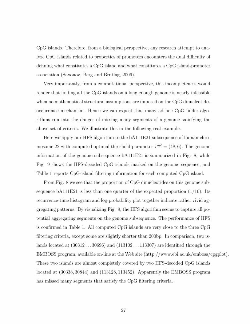
above set of criteria. We illustrate this in the following real example.
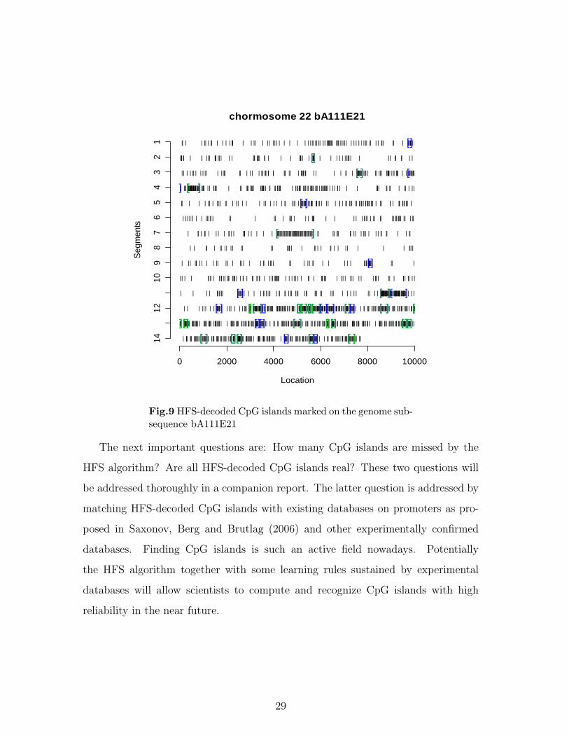
Here we apply our HFS algorithm to the bA111E21 subsequence of human chro-
mosome 22 with computed optimal threshold parameter τ opt = (48, 6). The genome
information of the genome subsequence bA111E21 is summarized in Fig. 8, while
Fig. 9 shows the HFS-decoded CpG islands marked on the genome sequence, and
Table 1 reports CpG-island filtering information for each computed CpG island.
From Fig. 8 we see that the proportion of CpG dinucleotides on this genome sub-
sequence bA111E21 is less than one quarter of the expected proportion (1/16). Its
recurrence-time histogram and log-probability plot together indicate rather vivid ag-
gregating patterns. By visualizing Fig. 9, the HFS algorithm seems to capture all po-
tential aggregating segments on the genome subsequence. The performance of HFS
is confirmed in Table 1. All computed CpG islands are very close to the three CpG
filtering criteria, except some are slightly shorter than 200bp. In comparison, two is-
lands located at (30312 . . . 30696) and (113102 . . . 113307) are identified through the
EMBOSS program, available on-line at the Web site (http://www.ebi.ac.uk/emboss/cpgplot).
These two islands are almost completely covered by two HFS-decoded CpG islands
located at (30338, 30844) and (113128, 113452). Apparently the EMBOSS program
has missed many segments that satisfy the CpG filtering criteria.
27

39891398913989139891296982969829698296982748427484274842748440645406454064540645
TTTTGGGGCCCCAAAA
128431284312843128431043710437104371043778397839783978398772877287728772TTTT
7396739673967396793979397939793955525552555255528811881188118811GGGG
9259925992599259165516551655165570437043704370439526952695269526CCCC
103931039310393103939666966696669666705070507050705013536135361353613536AAAA
TTTTGGGGCCCCAAAA
0120174.0137717
1655ˆ==
CGP
0.0 0.5 1.0 1.5 2.0 2.5 3.0
-3.0
-2.5
-2.0
-1.5
distance(log-scale,base=10)
Pro
bab
ility(l
og
-sca
le,b
ase
=1
0)
(a)
(c)
(b)
(d)
recurrence time
Pro
ba
bility
0 200 400 600 800 1000 1200
0.0
00
0.0
05
0.0
10
0.0
15
0.0
20
0.0
25
0.0
30
0.0
35
Fig.8 Summarized information of the genome subsequence bA111E21. (a) theA,G,T, and C nucleotides proportions; (b) 16 dinucleotides contents; (c) the re-currence time of CpG dinucleotides and the maximum entropy distribution basedon average recurrence time 1/PGC and the red line for maximum entropy Geometricdistribution; (d) the same comparison of panel (c) on log-probability vs log-lengthscales.
28
chormosome 22 bA111E21
Location
Segm
ents
0 2000 4000 6000 8000 10000
1412
109
87
65
43
21 || | | || | || | | | | ||| | | || | || ||| | | | | | | ||| || || || ||||||||| |||| ||||| | | | | | ||| || | | ||| || | ||||||||
|||||| | || ||| |||| ||| | | ||| |||| || | | | ||||| | ||||||||| | | | | | |||||| | || || || | |
|| | | || | | | || | |||| || | | | | ||| ||||| || ||| || | |||||||| | | | | || | ||||||||||||||||| || ||| ||||||| ||| |||| | | |||||||||||
|| ||| |||||||||||||||||||||||||||||||||||||| ||||| || ||||| | || ||| ||||| |||||||| || || |||||| | ||||||| |||||| |||||||| | |||||||| | | | || | | | |||| || || | || | ||
|| | | | || | ||| || | || | | | || | | | | || ||||| | ||||||||||||||||| ||||| | || | || | ||| ||| || ||||| ||||||||| | || || | ||| ||||||| |
| || || || | | ||||| | || | || | ||| | | | ||||| | | | | | |||| | || || || ||||||| || | ||
| || | || | | | | || | | |||| | | | | | ||||||||||||||||||||||||||||||||||||||||||||||||||| || || ||| || || | ||| | | | || || | | ||
| | || | || || || || || |||||| | || | | || | | || | | | ||||
| || ||| | | | | || || | || | | | || | || | ||| | || || | | | | | ||||| ||||||||| || |
|| | | |||| | |||| || ||| ||||| | || | || |||| | | || |||||||| | | | || | | || | |||||| | || | ||| | | | ||| | || | ||| || | |
| | | | ||||||| ||||||||| | | | || || || | || || | || ||| ||| ||| || | || | | | | | || | | |||||||||||||||||||||||||||||||||||||||||||||||||||||||||||||||||||||||| | |
| | | ||| | | |||||||||| | || | | | ||| ||||||| ||||||||||||||||||||||||||||||||| |||||||||| ||||||||||||||||| |||| |||||| ||||||||||||||||||||||||||||||| |||||||||||||||||||||||||||||||||||||||||||||| ||||||||||||||||||||||||||||| | || ||| |||||||||||||||||||||||| |||| ||||||| ||||| ||| |||
|||| ||||||||||||||| |||||||||| | ||||| ||||| |||||||||| | |||||| |||| |||||| |||| |||| |||||||||||||||||| | ||| || |||||||||||||||||||||||||||| |||| ||| || |||| |||| ||||||| |||||||||||||||| ||| ||||||| |||||| ||||| ||||||||| | |||||| |||| |||||| ||| ||||||||||||||||||||||||
| ||| ||| |||||||||||||||||||| |||| |||| ||||||| |||||||||||| ||||||||||||||||| |||||||||| | |||||| ||||| |||||||||| | ||||||| |||| |||||| |||||||||||||||||||||||||| | | ||| ||| |||||||||||||||||||||||||||| ||
[][][]
[ ][ ] [] [ ][ ]
[ ]
[ ][ ]
[]
[ ] [ ][ ][ ][ ] [][][ ][ ][] [][][ ][ ][][][ ][ ][ ][ ] [ ][ ][] [ ][ ] [
][
][][] [][] [ ][ ] [][][][] [ ][ ][][][ ][ ] [][][ ][ ] [] [ ][ ][] [ ][ ]
Fig.9 HFS-decoded CpG islands marked on the genome sub-sequence bA111E21
The next important questions are: How many CpG islands are missed by the
HFS algorithm? Are all HFS-decoded CpG islands real? These two questions will
be addressed thoroughly in a companion report. The latter question is addressed by
matching HFS-decoded CpG islands with existing databases on promoters as pro-
posed in Saxonov, Berg and Brutlag (2006) and other experimentally confirmed
databases. Finding CpG islands is such an active field nowadays. Potentially
the HFS algorithm together with some learning rules sustained by experimental
databases will allow scientists to compute and recognize CpG islands with high
reliability in the near future.
29

Table 1 Locations of CpG-islands identified by HFS algorithm with three filteringinformation.
Lstar 9721 15624 27553 29719 30338 45157 64127 88033 102484 108564
Lstop 9867 15736 27770 30019 30844 45394 65682 88179 102664 108900
length > 200 147 113 218 301 507 238 1556 147 181 337
GC content > 50% 0.544218 0.557522 0.555046 0.538206 0.65286 0.579832 0.522494 0.469388 0.436464 0.715134
O/E ratio > 0.6 0.572549 0.941176 0.675057 0.567108 0.700123 0.505115 0.637363 1.055104 0.833333 0.724138
Lstar 109011 111560 112960 113128 113517 115022 115186 115490 115648 116017
Lstop 109652 111759 113017 113452 113630 115126 115371 115565 115956 116236
length > 200 642 200 58 325 114 105 186 76 309 220
GC content > 50% 0.680685 0.47 0.706897 0.652308 0.640351 0.666667 0.612903 0.710526 0.631068 0.568182
O/E ratio > 0.6 0.492036 0.8284 0.87468 0.728155 0.523552 0.700337 0.699874 0.652174 0.655808 0.570313
Lstar 116296 117071 117280 118553 119964 120173 123222 123441 124851 126262
Lstop 116547 117215 117416 118840 120043 120310 123366 123567 125138 126341
length > 200 252 145 137 288 80 138 145 127 288 80
GC content > 50% 0.607143 0.655172 0.591241 0.576389 0.575 0.630435 0.648276 0.598425 0.583333 0.575
O/E ratio > 0.6 0.568467 0.609023 0.56044 0.613248 1.781955 0.88961 0.555985 0.593407 0.602941 1.781955
Lstar 126472 129505 129714 130897 132224 132456 134473 135525 135734 137207
Lstop 126611 129649 129850 131130 132333 132604 134592 135669 135852 137440
length > 200 140 145 137 234 110 149 120 145 119 234
GC content > 50% 0.621429 0.655172 0.59854 0.589744 0.572727 0.624161 0.4 0.662069 0.630252 0.589744
O/E ratio > 0.6 0.982065 0.614509 0.665734 0.62973 0.963384 0.979669 1.342105 0.671016 0.59 0.62973
7 Discussion
The HFS algorithm is proposed in this paper as a brand-new method of nonpara-
metric decoding for lengthy discrete time series. We reveal that HFS indeed has
high potential for decoding a binary state space vector through the evidence derived
from computer experiments and real genetic data analysis on CpG islands. Since
it requires no structural assumptions, its performance naturally is very robust and
free of systematic bias. For the same reason, its spectrum of applicability will be
rather wide.
Rigorous and theoretical developments for the HFS algorithm, beyond the in-
tensity change-point perspective considered here, will be further studied from the
30

perspectives of coding and data compression and Rissanen’s statistical complex-
ity. The fact that its construction rests on a hierarchy of recurrent time sequences
and distributions seems solid enough to allow it to be able to bring out dynamic
patterns of the observed time series, especially the aggregating pattern of certain
chosen events. This objective segmentation algorithm can be further extended to
decoding discrete time series generated from non-autonomous systems with internal
state variables taking values for more than two states. The computer experimental
results reported here also raise important theoretical and practical issues regarding
the robustness of the Viterbi algorithm as the most popular decoding technique.
More future research effort and attention is necessary to adequately address these
issues.
We further discuss why the Viterbi and its variant algorithms are not applicable
in the CpG island example. Originally the genome subsequence bA111E21 is a
symbolic string of A,G,T, and C (nucleotides). So there are 16 possible pairs of
dinucleotides, and one of them, the CG ordered pair, is defined as an event of interest.
There are two deterministic constraints: 1) given the previous symbol, there are only
4 possible dinucleotides to be seen, not 16; 2) after observing a CpG, the next pair
is certainly not be a CpG. To a great extent, these constraints disqualify the Viterbi
and its variant algorithms as natural candidates for decoding. It is worth noting that
these constraints have no impact at all on our HFS algorithm. We simply represent
the genome sequence as a 0-1 digital string, as in Fig. 9. The HFS algorithm takes
the 0-1 string as its data and performs the decoding computations. This is the great
advantage of our HFS algorithm.
Heuristically, the CpG island example is not particular; indeed all dynamic
programming-based decoding techniques are prone to sensitivity to the structural
assumptions on the state variable S(t), especially when analyzing lengthy dynamic
time series. Hence a non-parametric decoding algorithm would be not only desirable,
but also crucial in scientific endeavors.
31

Variant versions of our nonparametric decoding computations have been suc-
cessfully applied to the dissection of the circadian rhythmic cycles of the cockroach,
and to the identification of coherent emotional response variables of human subjects
when watching a series of films with different intensities of emotional stimuli. Cer-
tainly its applicability in behavioral study, where it was developed, is still pending.
Many other applications are explored as well at this stage.
8 References:
Bird, A. P. (1986). CpG island and the function of DNA methylation. Nature,
321, 209-213.
Bock, C., Walter, J., Paulsen, M., and Lengauer, T. (2006). CpG island mapping
by Epifenome prediction. PLoS Computational Biology, 6, 1055-1069.
Draper, D. (1995). Assessment and propagation of model uncertainty (with dis-
cussion). J. Roy. Stat. Soc. Ser. B57, 45-97.
Durbin, R. Eddy, S. Krogh, A. and Mitchison, G. (1998) Biological Sequence Anal-
ysis. Cambridge Univ. Press. Cambridge, UK.
Durbin, J. and Koopman, S. J. (2001) Time Series Analysis by State Space Meth-
ods. Oxford University Press, New York.
Fushing, H., Hwang, C. R., Lee, H. C., Lan, Y. C. and Horng, S. B. (2006) Testing
and mapping non-stationarity in animal behavioural processes: a case study
on an individual female bean weevil. J. Theor. Biol. 238, 805-816.
Gardiner-Garden, M. and Frommer, M (1987). CpG island in vertebrate genomes.
J. Mol. Biol. 196, 261-282.
Geman, S. and Kochanek, K. (2001) Dynamic programming and the graphic rep-
resentation of error-correcting codes. IEEE Trans. Inform. Theory, IT-47,
549-568.
32

Hamilton, J. D. (2005) What’s real about the business cycles? Federal Reserve
Bank of St. Louis Review, 87(4), 435-452.
Hsieh, F. and Turnbull, B. (1996). Non- and semi- parametric estimation of the
receiver operating characteristics (ROC) curve. Ann Statist. 24, 25-40.
Jaynes, E. T. (1957a). Information theory and statistical mechanics. Phys. Rev.
106, 620-630.
Jaynes, E. T. (1957b). Information theory and statistical mechanics II. Phys. Rev.
108, 171-190
Kalman, R. E. (1960). A new approach of linear filtering and prediction problems.
J. Basic Engineering. Transactions ASMA. Series D, 82, 35-45.
Laird, P. W. (2005). Cancer epigenetics. Hum. Mol. Genet. 14 R65-R76.
Lanterman, A. D. (2001). Schwarz, Wallace and Rissanen: Interwining themes
in theories of model order estimation. International Statistical Review, 69,
185-212.
Lee, T.C.M. (2001). An introduction to coding theory and the two-part minimum
description length principle. Inter. Statist. Rev., 69, 169-183.
Manuca, R. and Savit, R. (1996) Stationarity and nonstationarity in time series
analysis. Physica D. 99, 134-161
Rabiner, L. R. (1989) A tutorial on Hidden Markov models and selected applica-
tions in speech recognition. Proc. of IEEE 77, 257-286.
Rissanen, J. (1996). Fisher information and stochastic complexity. IEEE Trans.
Inform. Theory, IT-42, 40-47.
Rissanen, J. (1997). Stochastic complexity in learning. J. Computer and System
Sciences, 55, 89-95.
33

Saxonov, S. Berg, P. and Brutlag, D. (2006). A genome-wide analysis of CpG dinu-
cleotides in the human genome distinguishes two distinct classes of promoters.
Proc. Natl. Acad. Sci. U.S.A, 103, 1412-1417.
Schawrz, G. (1978) Estimating the dimension of a model. Ann. Stat. 6, 461-464.
Takai D. and Jones, P. A. (2002) Comprehensive analysis of CpG island in human
chromosomes 21 and 22. Proc. Natl. Acad. Sci. U.S.A, 99, 3740-3745.
Viterbi, A. J. (1967). Error bounds for convolutional codes and an asymptotically
optimal decoding algorithm. IEEE Trans. Inform. Theory, IT-13, 260-269.
West, M. and Harrison, J. (1997) Bayesian Forecasting and Dynamic Models. (2nd
ed.) Springer, New York.
34