Sieci neuronowe – bezmodelowa analiza danych?

K. M. GraczykIFT, Uniwersytet Wrocławski

Poland

Abstract• Podczas seminarium opowiem o zastosowaniu jednokierunkowych

sieci neuronowych do analizy danych eksperymentalnych. W szczególności skupię uwagę na podejściu bayesowskim, które pozwala na klasyfikację i wybór najlepszej hipotezy badawczej. Metoda ta ma w naturalny sposób wbudowane tzw. kryterium „brzytwy Ockhama”, preferujące modele o mniejszym stopniu złożoności. Dodatkowym atutem podejścia jest brak wymogu używania tzw. zbioru testowego do weryfikacji procesu uczenia.

• W drugiej części seminarium omówię własną implementacje sieci neuronowej, zawierającą metody uczenia bayesowskiego. Na zakończenie pokaże moje pierwsze zastosowania w analizie danych rozproszeniowych.

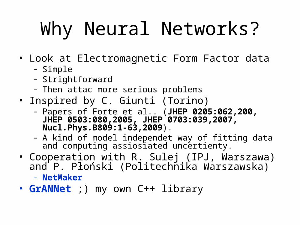
Why Neural Networks?

• Look at Electromagnetic Form Factor data– Simple– Strightforward– Then attac more serious problems

• Inspired by C. Giunti (Torino)– Papers of Forte et al.. (JHEP 0205:062,200, JHEP

0503:080,2005, JHEP 0703:039,2007, Nucl.Phys.B809:1-63,2009).

– A kind of model independet way of fitting data and computing assiosiated uncertienty.

• Cooperation with R. Sulej (IPJ, Warszawa) and P. Płoński (Politechnika Warszawska)– NetMaker

• GrANNet ;) my own C++ library

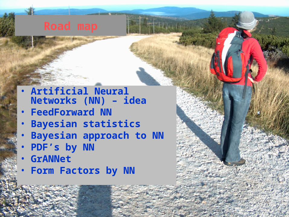
Road map

• Artificial Neural Networks (NN) – idea

• FeedForward NN• Bayesian statistics• Bayesian approach to NN• PDF’s by NN• GrANNet• Form Factors by NN

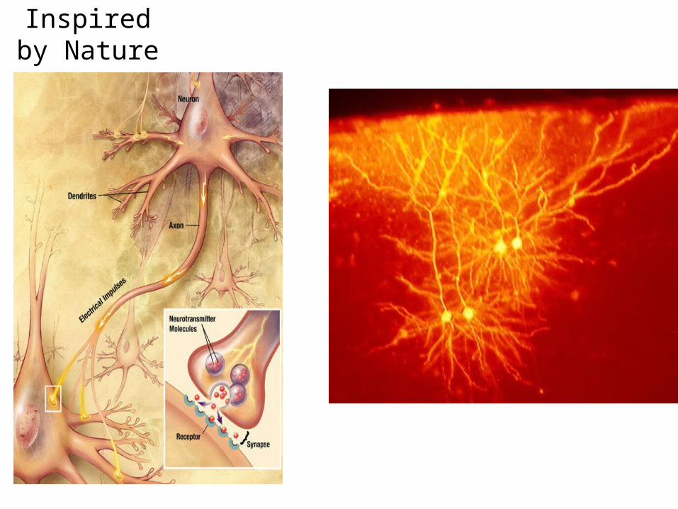
Inspired by Nature

Aplications, general list• Function approximation, or

regression analysis, including time series prediction, fitness approximation and modeling.

• Classification, including pattern and sequence recognition, novelty detection and sequential decision making.

• Data processing, including filtering, clustering, blind source separation and compression.

• Robotics, including directing manipulators, Computer numerical control.

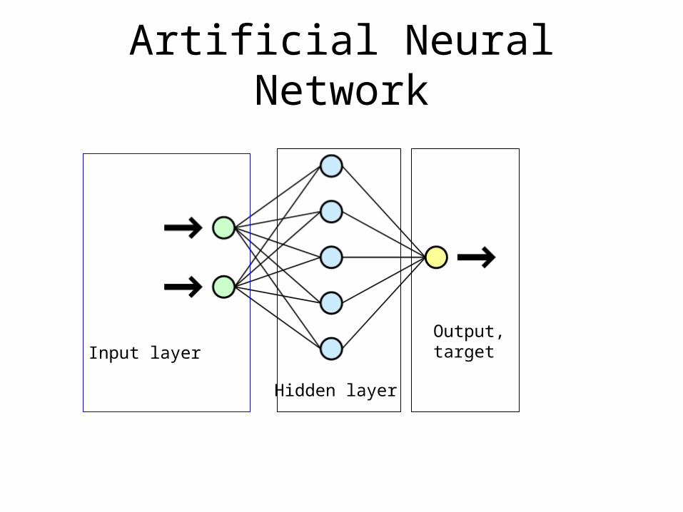
Artificial Neural Network

Input layer

Hidden layer

Output, target

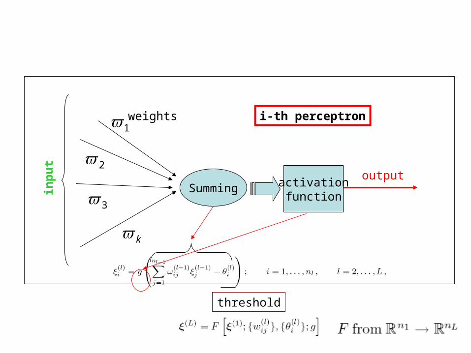
threshold

Summingoutput

activationfunction

inp

ut

1

2

3

k

i-th perceptronweights

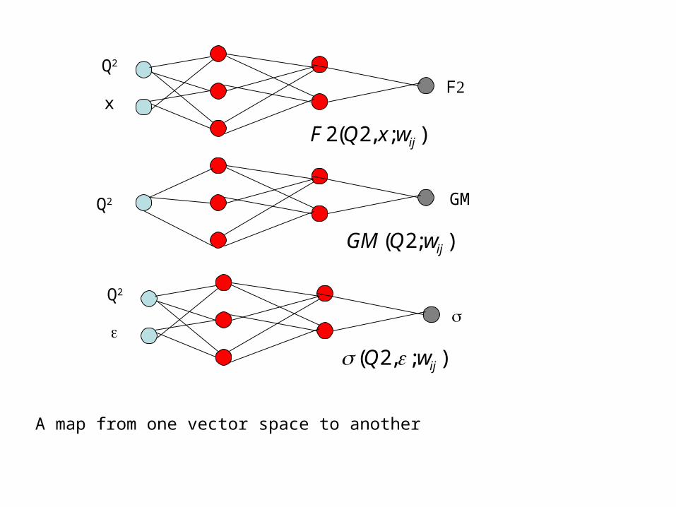
Q2

xF

);,2(2 ijwxQF

Q2

);,2( ijwQ

);2( ijwQGM

Q2 GM

A map from one vector space to another

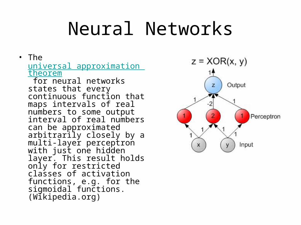
Neural Networks• The

universal approximation theorem for neural networks states that every continuous function that maps intervals of real numbers to some output interval of real numbers can be approximated arbitrarily closely by a multi-layer perceptron with just one hidden layer. This result holds only for restricted classes of activation functions, e.g. for the sigmoidal functions. (Wikipedia.org)

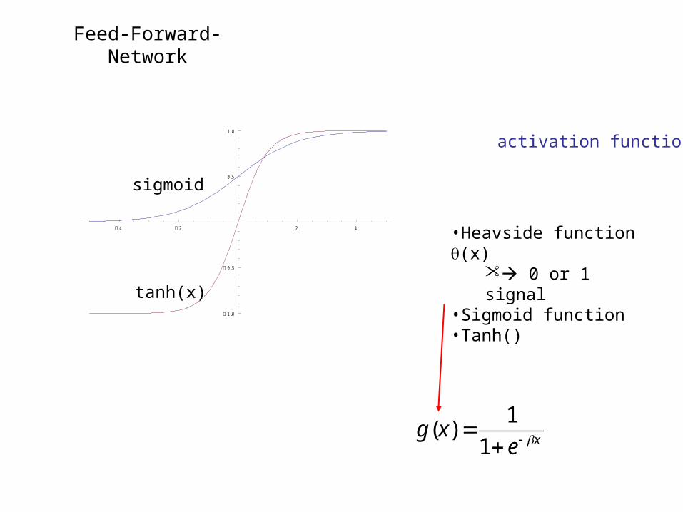
Feed-Forward-Network

activation function

•Heavside function (x) 0 or 1 signal

•Sigmoid function•Tanh()

xexg

1

1)(

4 2 2 4

1 .0

0 .5

0 .5

1 .0

tanh(x)

sigmoid

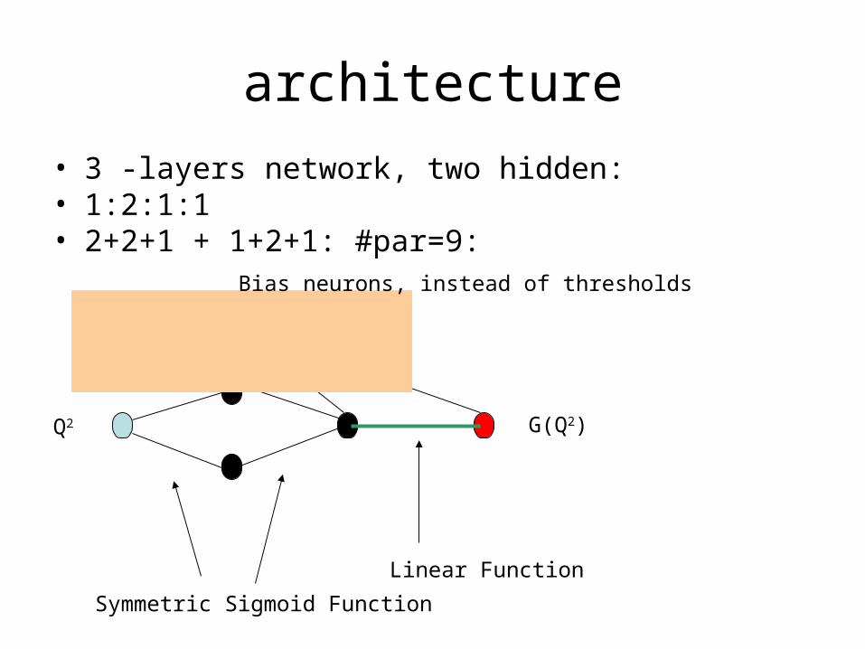
architecture

• 3 -layers network, two hidden:• 1:2:1:1• 2+2+1 + 1+2+1: #par=9:

Q2 G(Q2)

Linear Function

Symmetric Sigmoid Function

Bias neurons, instead of thresholds

Supervised Learning

• Propose the Error Function (Standard Error Function, chi2, etc, …, any continous function which has a global minimum)

• Consider set of the data

• Train given network with data marginalize the error function– Back propagation algorithms– Iterative procedure which fixes weights

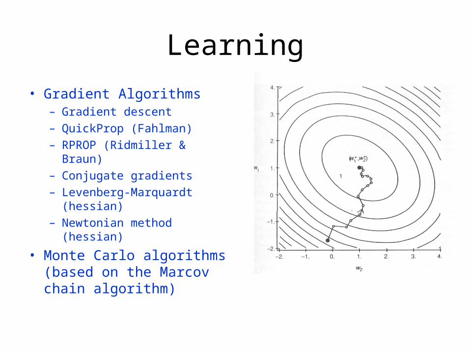
Learning

• Gradient Algorithms– Gradient descent– QuickProp (Fahlman)– RPROP (Ridmiller &

Braun)– Conjugate gradients– Levenberg-Marquardt

(hessian)– Newtonian method

(hessian)

• Monte Carlo algorithms (based on the Marcov chain algorithm)

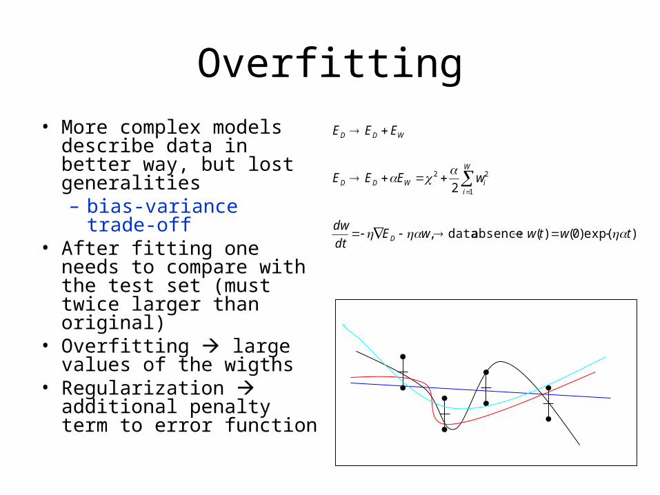
Overfitting

• More complex models describe data in better way, but lost generalities– bias-variance trade-off

• After fitting one needs to compare with the test set (must twice larger than original)

• Overfitting large values of the wigths

• Regularization additional penalty term to error function

)exp()0()(absence data,

2 1

22

twtwwEdt

dw

wEEE

EEE

D

W

iiWDD

WDD

Fitting data with Artificial Neural Networks

‘The goal of the network training is not to learn on exact representation of the training data itself, but rather to built statistical model for the process which generates the data’

C. Bishop, Neural Networks for Pattern Recognation

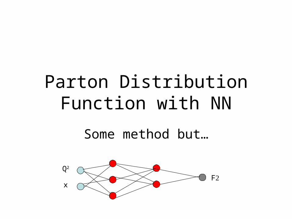
Parton Distribution Function with NN

Some method but…

Q2

xF

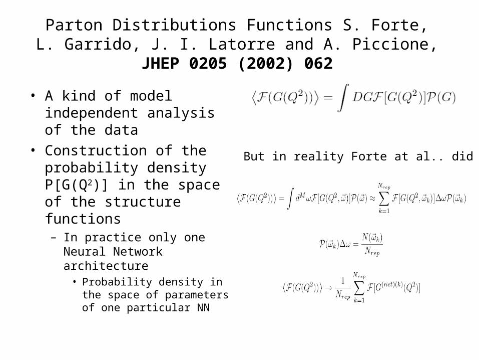
Parton Distributions Functions S. Forte, L. Garrido, J. I. Latorre and A. Piccione, JHEP 0205 (2002) 062

• A kind of model independent analysis of the data

• Construction of the probability density P[G(Q2)] in the space of the structure functions– In practice only one Neural

Network architecture• Probability density in the

space of parameters of one particular NN

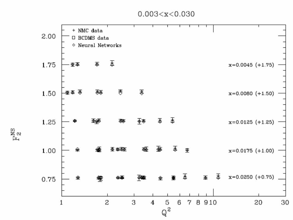
But in reality Forte at al.. did

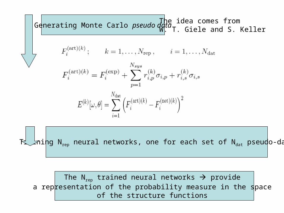
Training Nrep neural networks, one for each set of Ndat pseudo-data

Generating Monte Carlo pseudo data

The Nrep trained neural networks provide a representation of the probability measure in the space

of the structure functions

The idea comes fromW. T. Giele and S. Keller

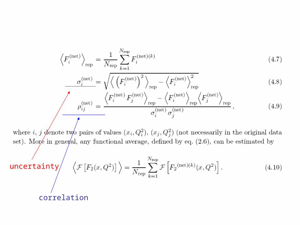
correlation

uncertainty

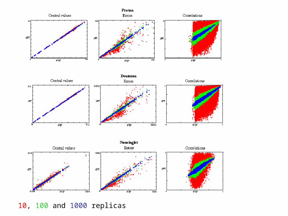
10, 100 and 1000 replicas

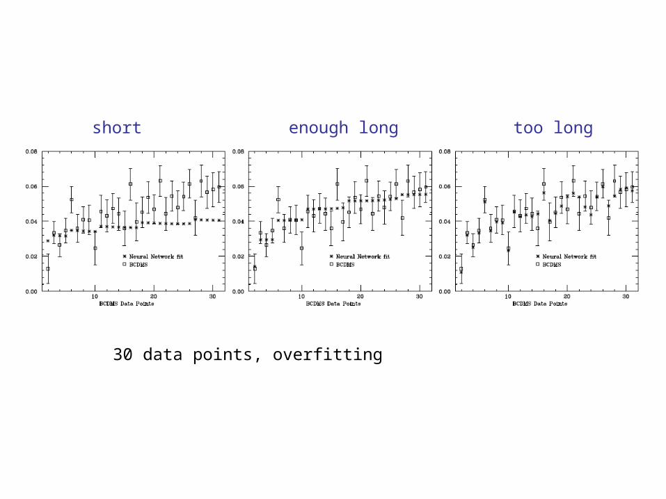
30 data points, overfitting

short enough long too long

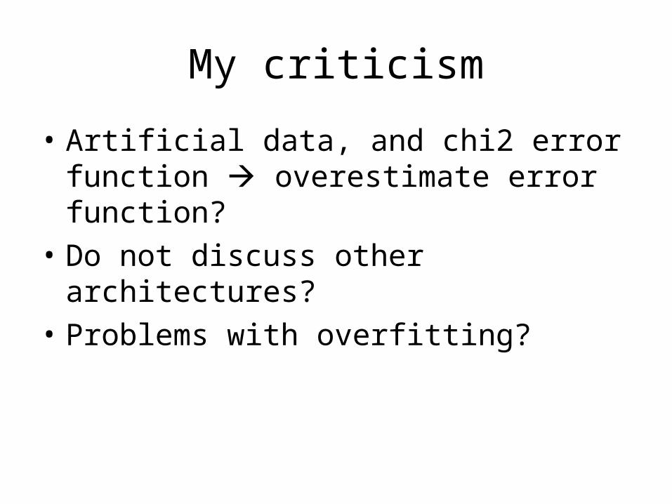
My criticism

• Artificial data, and chi2 error function overestimate error function?

• Do not discuss other architectures?

• Problems with overfitting?

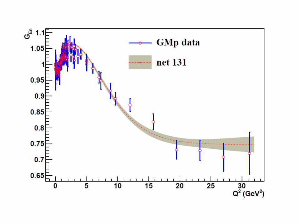
Form Factors with NN, done with FANN library

Applying Forte et al..

How to apply NN to the ep data

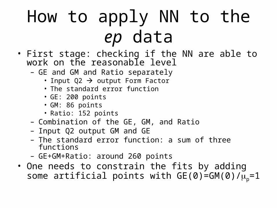
• First stage: checking if the NN are able to work on the reasonable level– GE and GM and Ratio separately

• Input Q2 output Form Factor• The standard error function• GE: 200 points• GM: 86 points• Ratio: 152 points

– Combination of the GE, GM, and Ratio– Input Q2 output GM and GE– The standard error function: a sum of three functions– GE+GM+Ratio: around 260 points

• One needs to constrain the fits by adding some artificial points with GE(0)=GM(0)/p=1

GMp

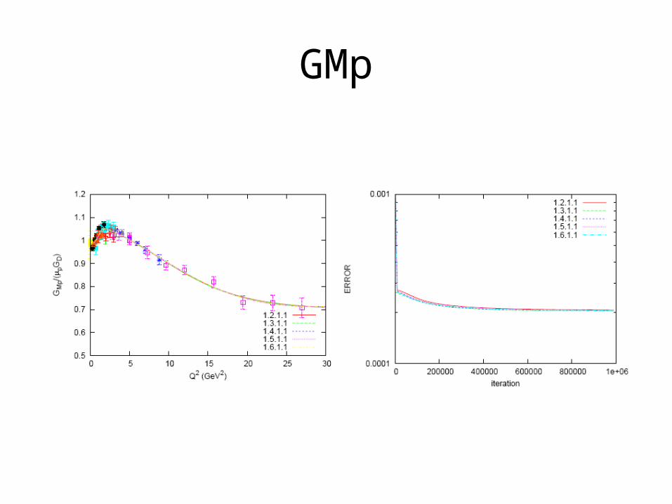
GMp

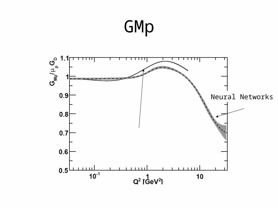
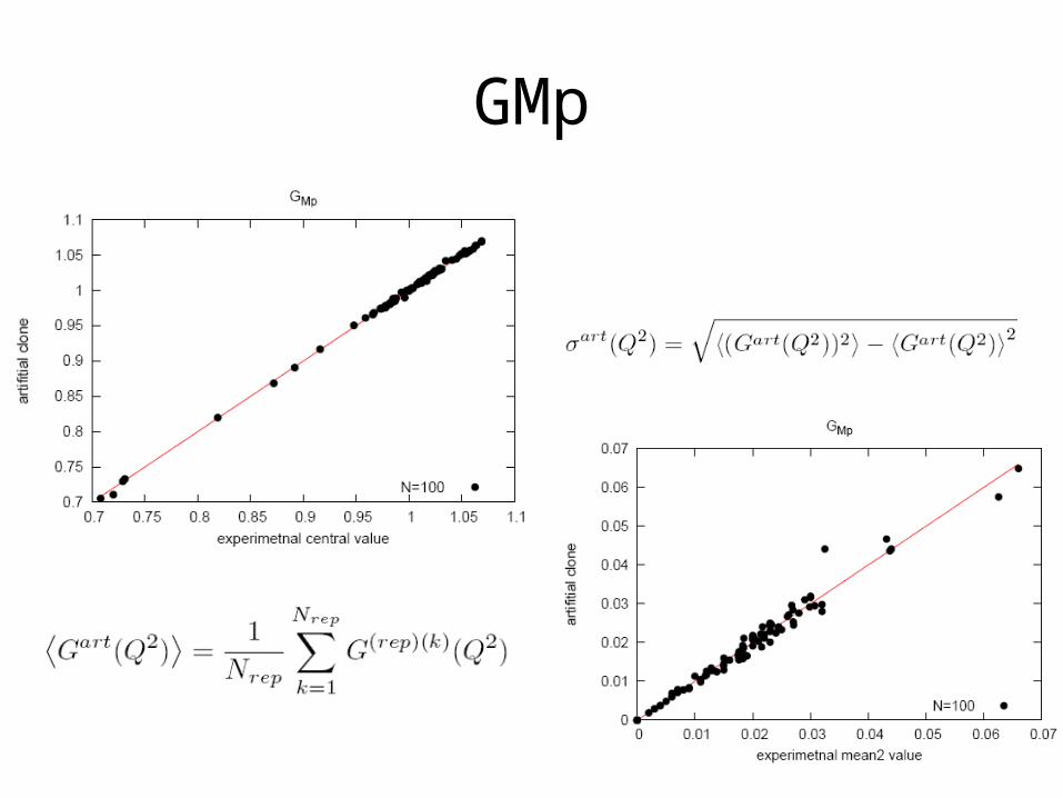
GMp

Fit with TPE (our work)

Neural Networks

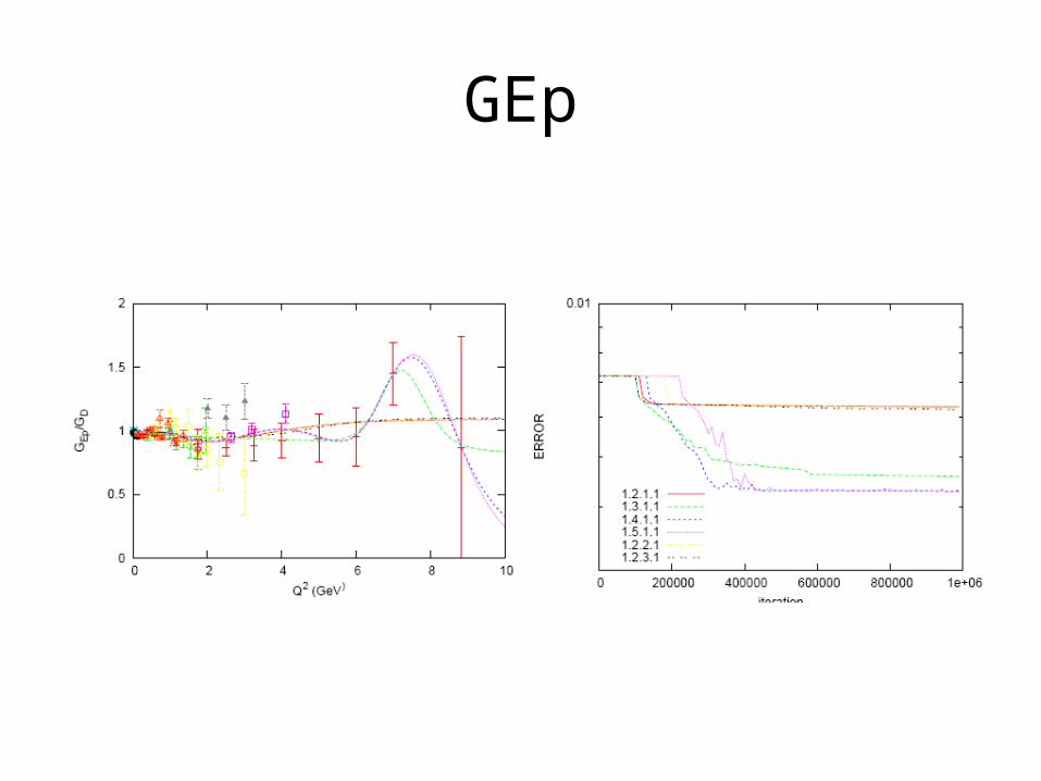
GEp

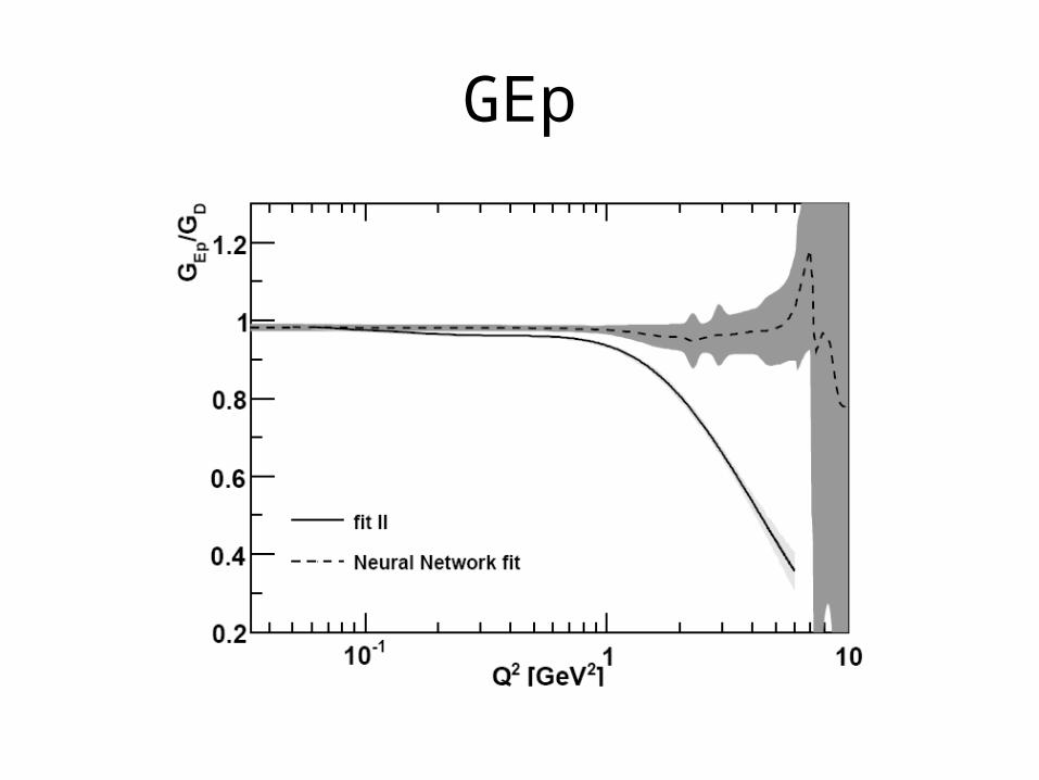
GEp

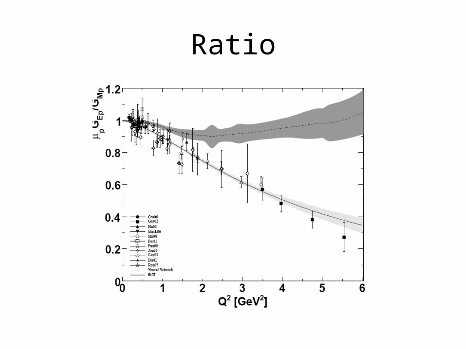
Ratio

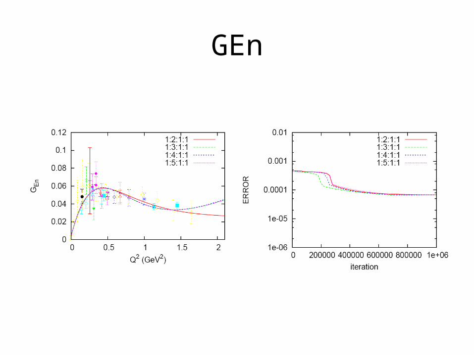
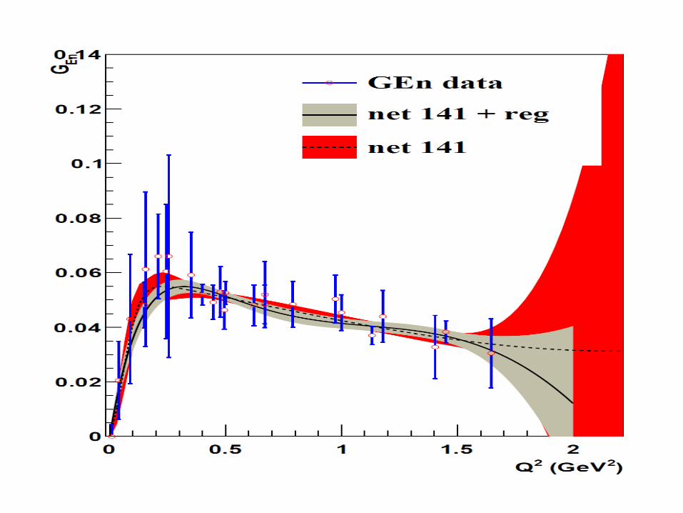
GEn

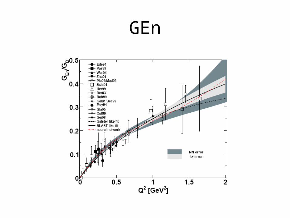
GEn

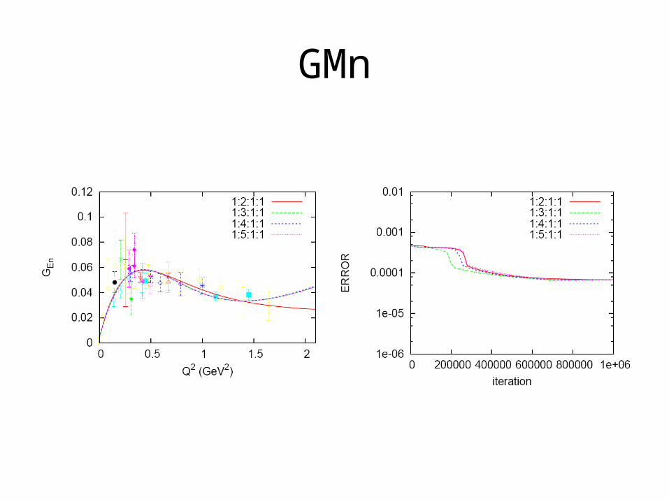
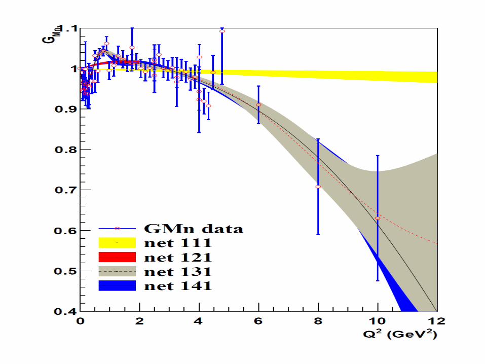
GMn

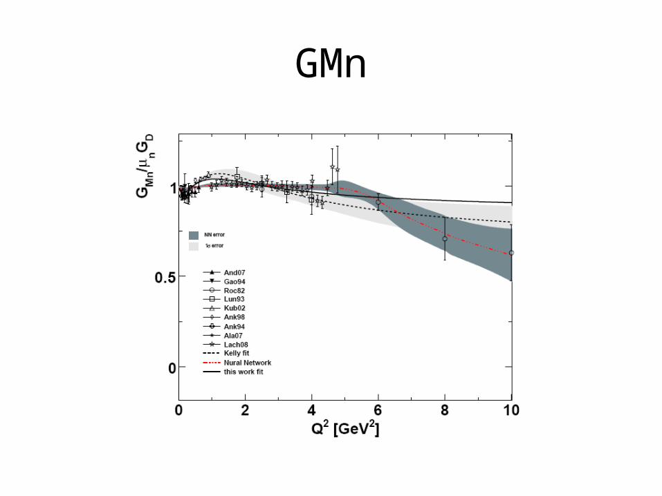
GMn

Bayesian Approach

‘common sense reduced to calculations’

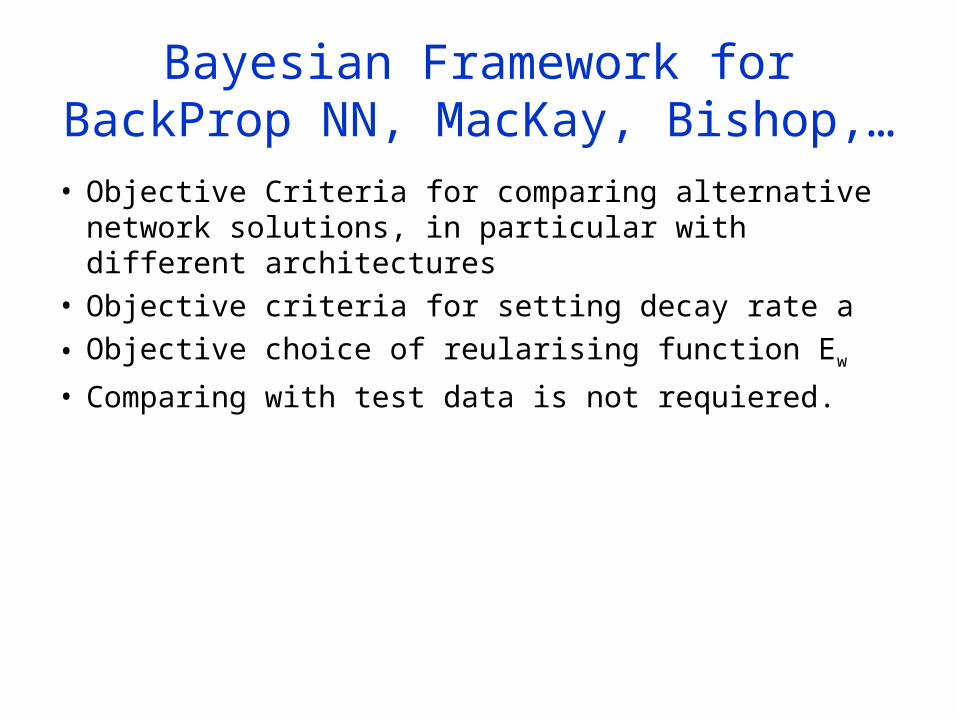
Bayesian Framework for BackProp NN, MacKay, Bishop,…

• Objective Criteria for comparing alternative network solutions, in particular with different architectures

• Objective criteria for setting decay rate a

• Objective choice of reularising function Ew

• Comparing with test data is not requiered.

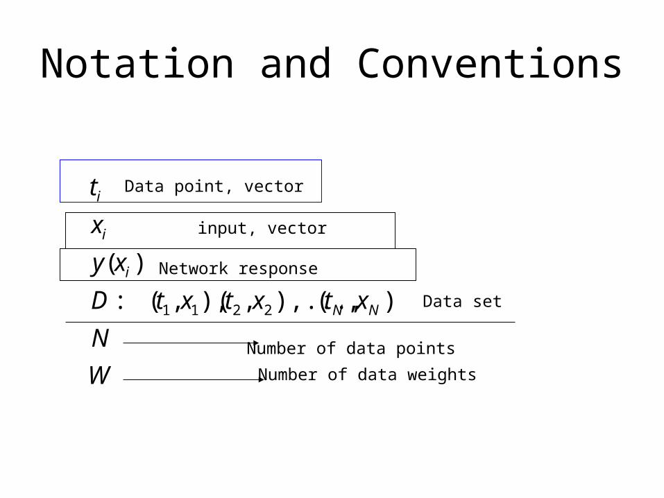
Notation and Conventions

W

N

xtxtxtD

xy

x

t

NN

i

i

i

),(),...,,(),,( :

)(

2211

Data point, vector

input, vector

Network response

Data set

Number of data points

Number of data weights

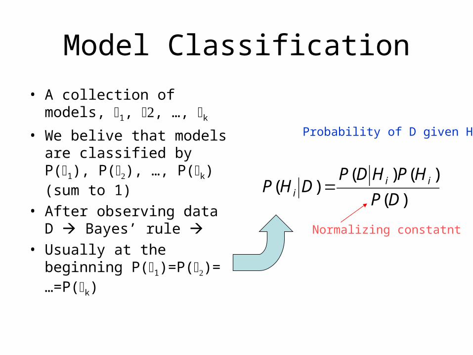
Model Classification

• A collection of models, 1, , …, k

• We belive that models are classified by P(1), P(), …, P(k) (sum to 1)

• After observing data D Bayes’ rule

• Usually at the beginning P(1)=P()= …=P(k)

)(

)()()(

DP

HPHDPDHP ii

i

Normalizing constatnt

Probability of D given Hi

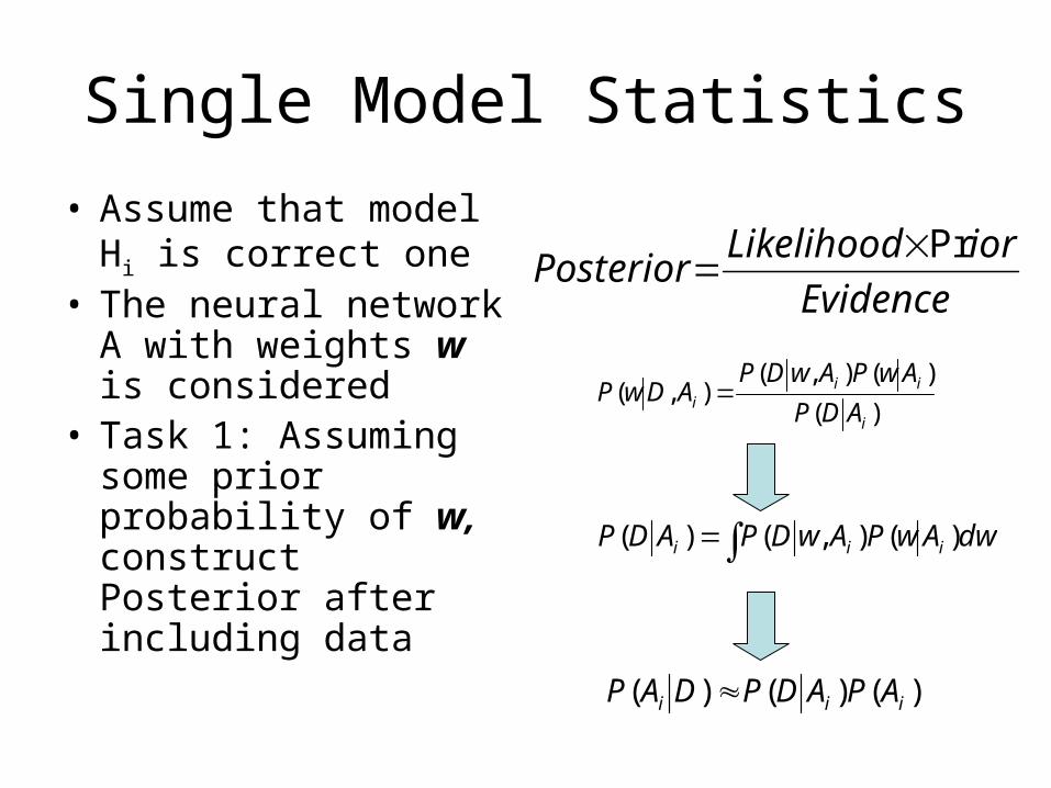
Single Model Statistics

• Assume that model Hi is correct one

• The neural network A with weights w is considered

• Task 1: Assuming some prior probability of w, construct Posterior after including data

)(

)(),(),(

i

iii ADP

AwPAwDPADwP

Evidence

iorLikelihoodPosterior

Pr

)()()( iii APADPDAP

dwAwPAwDPADP iii )(),()(

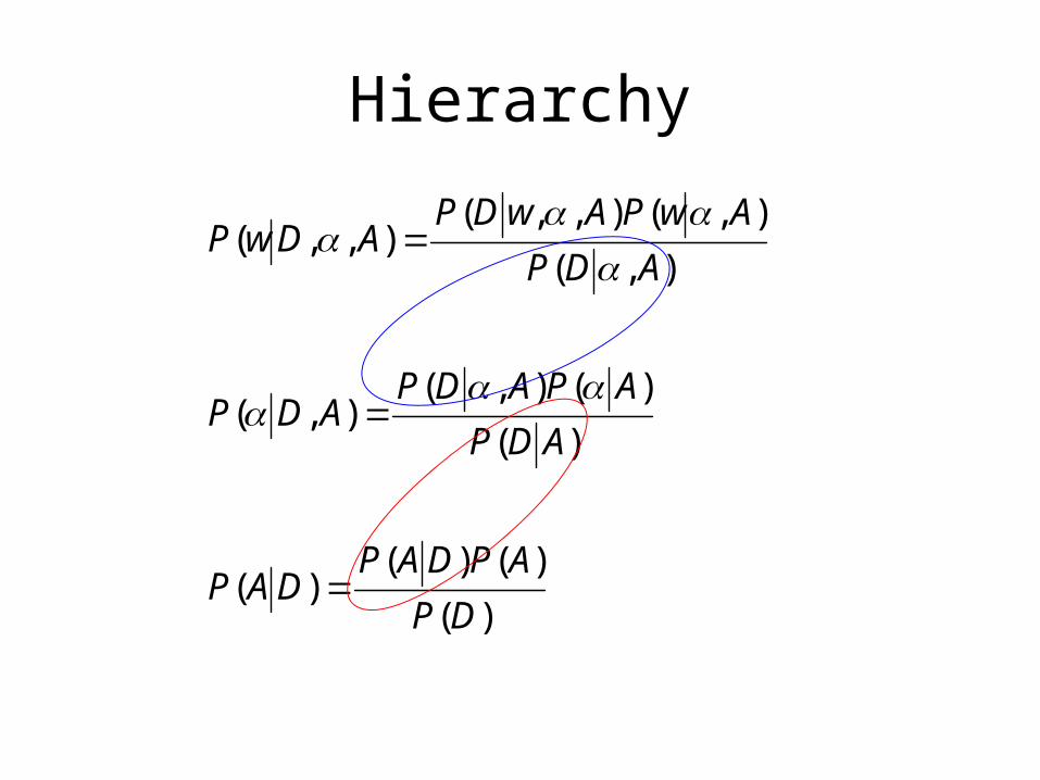
Hierarchy

)(

)()()(

)(

)(),(),(

),(

),(),,(),,(

DP

APDAPDAP

ADP

APADPADP

ADP

AwPAwDPADwP

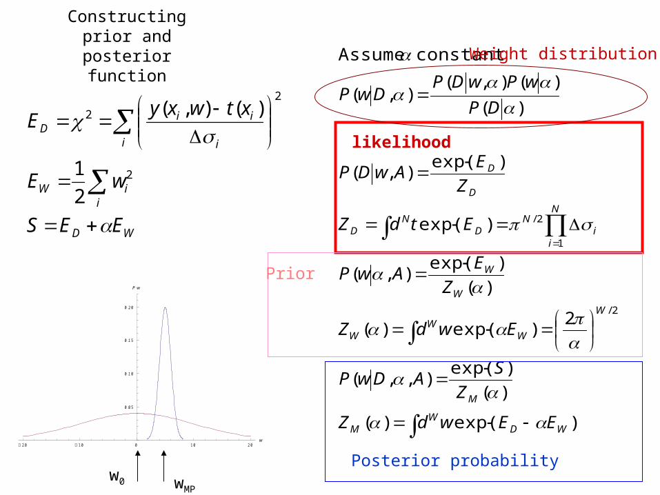
Constructing prior and posterior function

WD

iiW

i i

iiD

EES

wE

xtwxyE

2

2

2

2

1

)(),(

)exp()(

)(

)exp(),,(

2)exp()(

)(

)exp(),(

)exp(

)exp(),(

)(

)(),(),(

constant Assume

2/

1

2/

WDW

M

M

W

WW

W

W

W

N

ii

ND

ND

D

D

EEwdZ

Z

SADwP

EwdZ

Z

EAwP

EtdZ

Z

EAwDP

DP

wPwDPDwP

likelihood

Prior

Posterior probability 20 10 0 10 20

w

0 .05

0 .10

0 .15

0 .20

P w

wMPw0

Weight distribution!!!

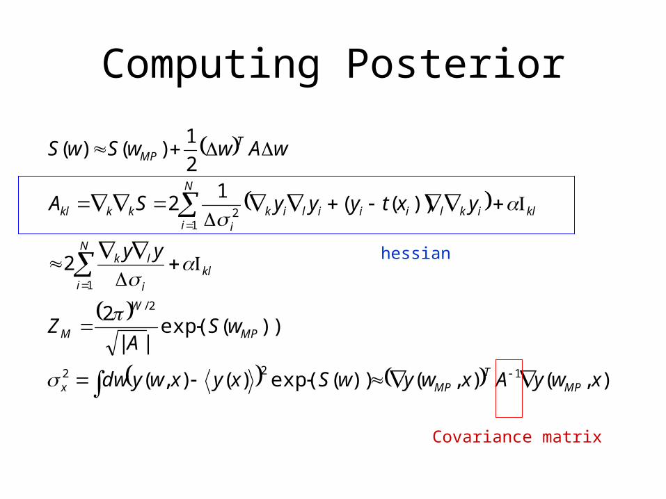
Computing Posterior

),(),())(exp()(),(

))(exp(||

2

2

))((1

2

2

1)()(

122

2/

1

12

xwyAxwywSxyxwydw

wSA

Z

yy

yxtyyySA

wAwwSwS

MPT

MPx

MP

W

M

kl

N

i i

lk

kl

N

iikliiilik

ikkkl

TMP

hessian

Covariance matrix

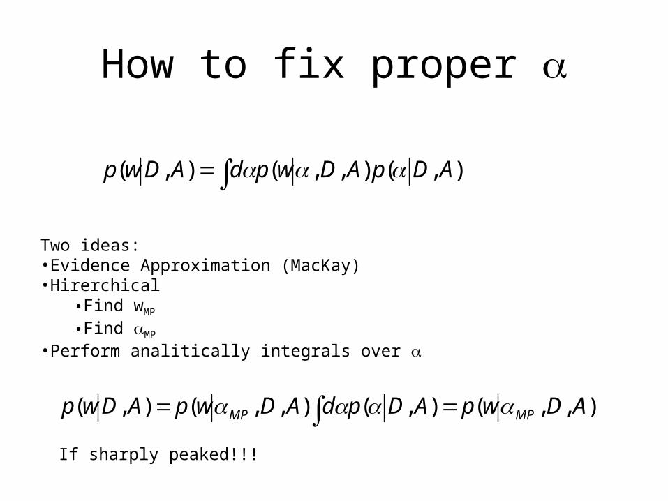
How to fix proper

),,(),(),,(),( ADwpADpdADwpADwp MPMP

Two ideas:•Evidence Approximation (MacKay)•Hirerchical

•Find wMP

•Find MP •Perform analitically integrals over

),(),,(),( ADpADwpdADwp

If sharply peaked!!!

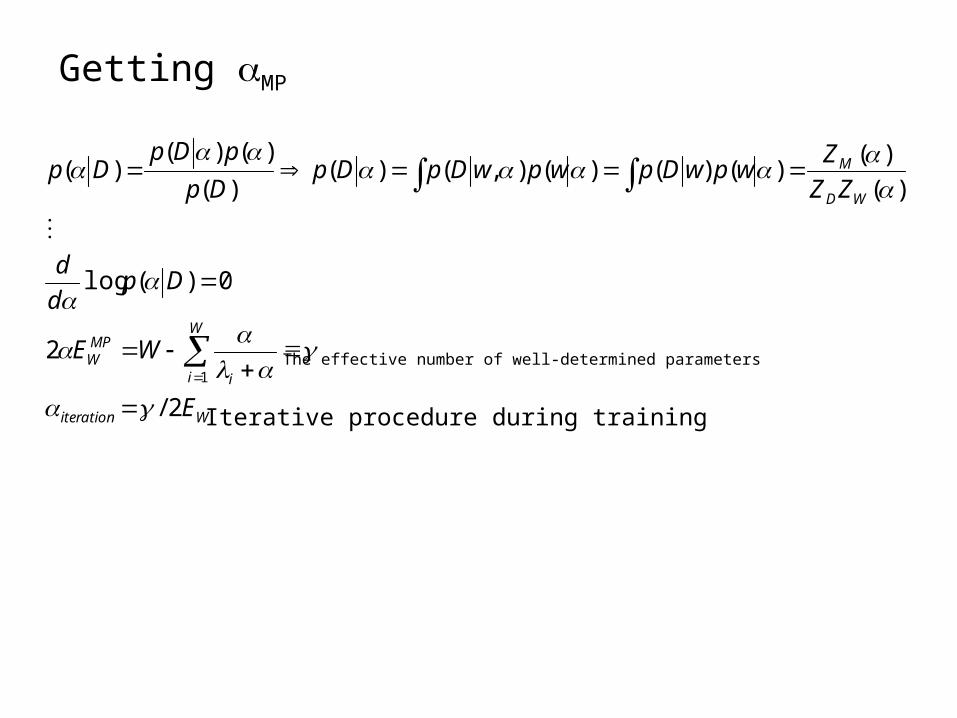
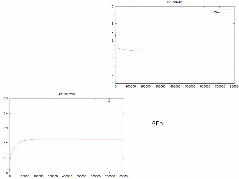
Getting MP

Witeration

W

i i

MPW

WD

M

E

WE

Dpd

d

ZZ

ZwpwDpwpwDpDp

Dp

pDpDp

2/

2

0)(log

)(

)()()()(),()(

)(

)()()(

1

The effective number of well-determined parameters

Iterative procedure during training

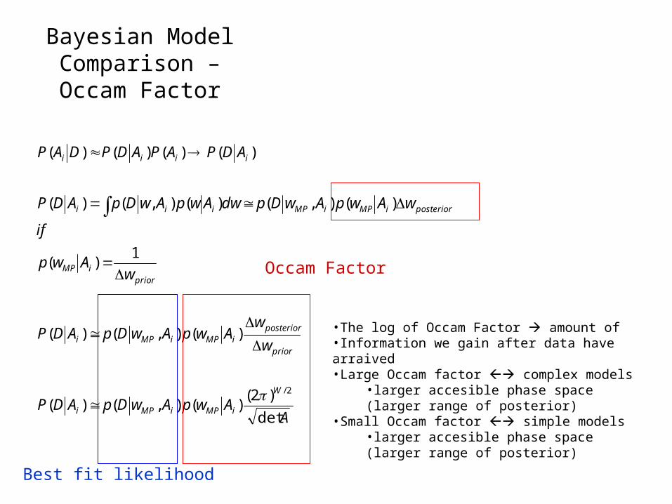
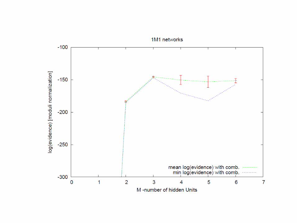
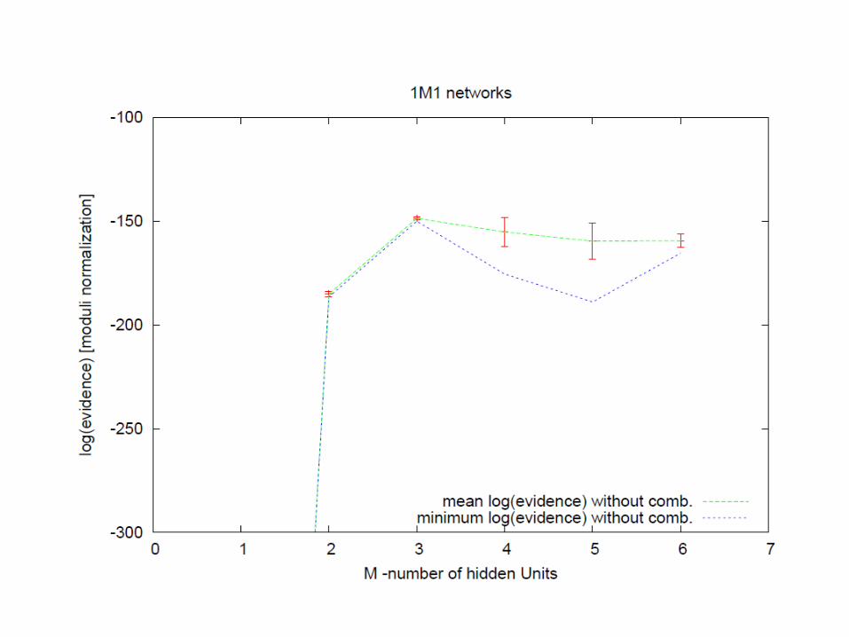
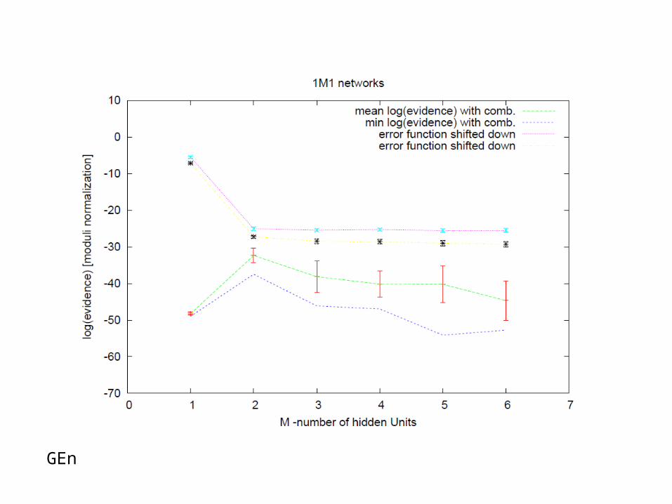
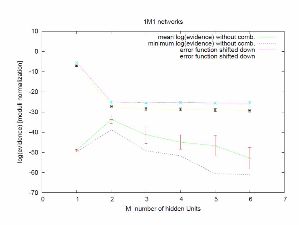
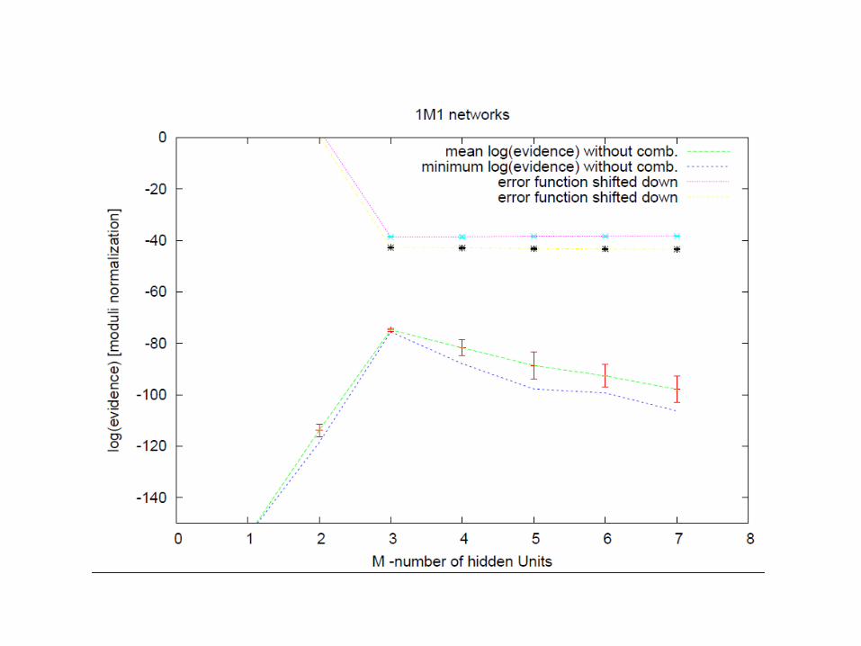
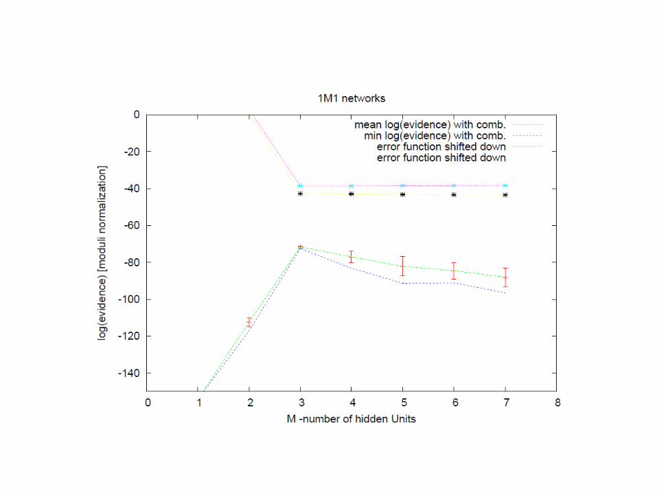
Bayesian Model Comparison – Occam Factor

AAwpAwDpADP

w

wAwpAwDpADP

wAwp

if

wAwpAwDpdwAwpAwDpADP

ADPAPADPDAP

W

iMPiMPi

prior

posterioriMPiMPi

prioriMP

posterioriMPiMPiii

iiii

det

)2()(),()(

)(),()(

1)(

)(),()(),()(

)()()()(

2/

Occam Factor

Best fit likelihood

•The log of Occam Factor amount of•Information we gain after data have arraived•Large Occam factor complex models

•larger accesible phase space (larger range of posterior)

•Small Occam factor simple models•larger accesible phase space (larger range of posterior)

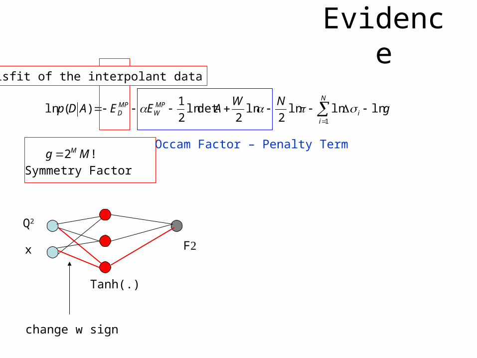
Evidence

!2

lnlnln2

ln2

detln2

1)(ln

1

Mg

gNW

AEEADp

M

N

ii

MPW

MPD

Symmetry Factor

Q2

x F

change w sign

Tanh(.)

Misfit of the interpolant data

Occam Factor – Penalty Term

What about cross sections

• GE and GM simultaneously, – Input Q2 and cross sections

• Standard error function• the chi-2-like function, with the covariance matrix obtained

from the Rosenbluth separation

– Possibilities:• The set of Neural Networks becomes a natural distribution of

the differential cross sections• One can produce artificial data in the wide range of the

epsilon and perform the Rosenbluth separation, searching the nonlinearities of R in the epsilon dependence.

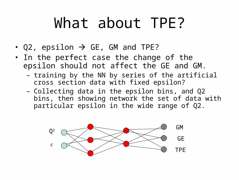
What about TPE?

• Q2, epsilon GE, GM and TPE?• In the perfect case the change of the epsilon should not

affect the GE and GM. – training by the NN by series of the artificial cross section data

with fixed epsilon?– Collecting data in the epsilon bins, and Q2 bins, then showing

network the set of data with particular epsilon in the wide range of Q2.

Q2

GM

GE

TPE

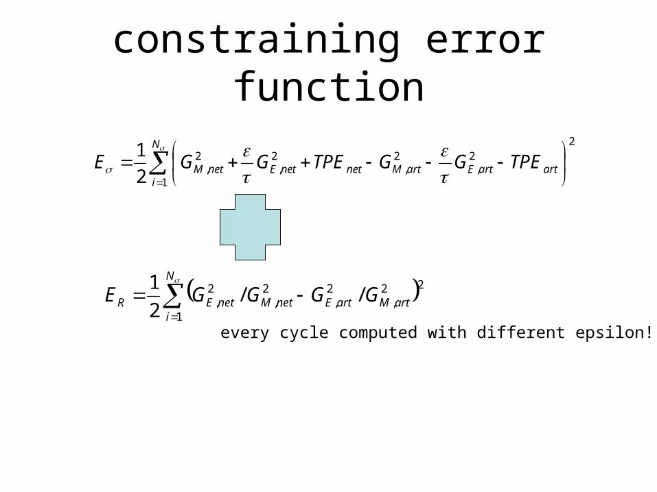
constraining error function

N

iartartEartMnetnetEnetM TPEGGTPEGGE

1

22

,2

,2

,2

,2

1

N

iartMartEnetMnetER GGGGE

1

22,

2,

2,

2, //

2

1

every cycle computed with different epsilon!

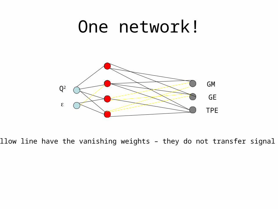
One network!

Q2

GM

GE

TPE

Yellow line have the vanishing weights – they do not transfer signal

Q2

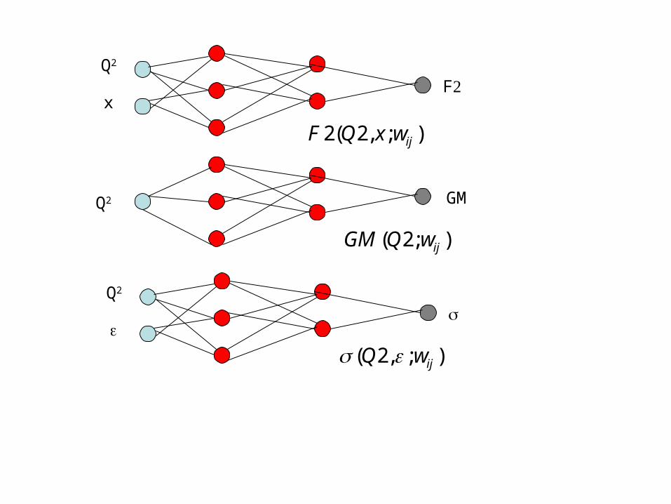
xF

);,2(2 ijwxQF

Q2

);,2( ijwQ

);2( ijwQGM

Q2 GM

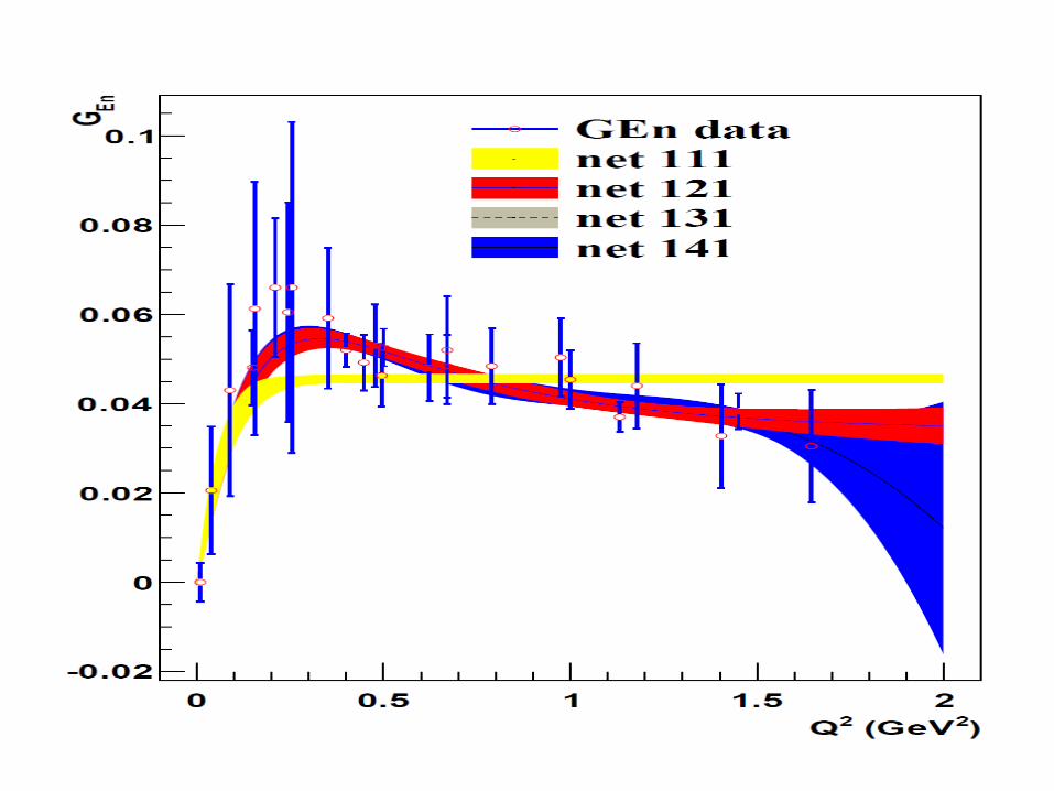
GEn

GEn

GMn

results

GEp

ddd

GMp