Optim LettDOI 10.1007/s11590-014-0740-z

ORIGINAL PAPER

Single machine serial-batching scheduling withindependent setup time and deteriorating jobprocessing times

Jun Pei · Xinbao Liu · Panos M. Pardalos ·Wenjuan Fan · Shanlin Yang

Received: 8 September 2013 / Accepted: 19 March 2014© Springer-Verlag Berlin Heidelberg 2014

Abstract This paper investigates the scheduling problems of a single serial-batchingmachine with independent setup time and deteriorating job processing times. Withthe assumption of deteriorating jobs, the job processing times are described by anincreasing function of their starting times. All the jobs are first partitioned into serialbatches and then processed on a single serial-batching machine. Before each batchis processed, an independent constant setup time is required. Two optimization algo-rithms are proposed to solve the problems of minimizing the makespan and the totalnumber of tardy jobs, respectively. Specifically, for the problem of minimizing thetotal completion time, two special cases with the smallest and the largest number ofbatches are studied, and an optimization algorithm is also presented for the specialcase without setup time.

J. Pei · X. Liu · W. Fan · S. YangSchool of Management, Hefei University of Technology, Hefei, China

J. Pei (B) · P. M. PardalosDepartment of Industrial and Systems Engineering, Center for Applied Optimization, Universityof Florida, Gainesville, USAe-mail: peijun@ufl.edu

X. Liu · S. YangKey Laboratory of Process Optimization and Intelligent Decision-Making of Ministry of Education,Hefei, China

P. M. PardalosLaboratory of Algorithms and Technologies for Networks Analysis, National Research UniversityHigher School of Economics, Moscow, Russia

W. FanDepartment of Computer Science, North Carolina State University, Raleigh, USA

123

J. Pei et al.

Keywords Serial-batching scheduling · Deteriorating jobs · Single machine · Setuptime

1 Introduction

In traditional scheduling problems, the processing times of jobs are assumed to befixed and independent constant values. However, in many production environments,we often encounter the situation that the job processing times vary with time. Sincethe scheduling problem with deteriorating jobs was first introduced by Gupta andGupta [1] and Browne and Yechiali [2], there has been additional research concerningvarious scheduling problems with deteriorating jobs. Batch production, as an importantprocessing way, exists in many scheduling environments. The types of the batch refer toparallel-batching and serial-batching. In recent years, the parallel-batching schedulingproblems with deteriorating jobs have been addressed in some papers, including Qi etal. [3], Li et al. [4], and Miao et al. [5,6].

The actual production scenario involving serial batches and deteriorating jobs canbe found in many manufacturing factories. As a practical example of the proposedscheduling model, the aluminum-making process in an aluminum plant is considered.In particular, cylindrical aluminum ingots are stored in a buffer awaiting the extrusionprocess after they are processed in a heating furnace. During the extrusion process, amold is required to assemble with the extrusion machine, which is a batch processingmachine that processes a batch of aluminum ingots for the extrusion process in theform of serial batches, i.e., aluminum ingots in the same batch are processed one afteranother. Before each batch of aluminum ingots is processed, a constant setup time isrequired. The processing time of an aluminum ingot depends on its type accordingto different customers’ requirements and the mold’s performance at the beginningof the process. The longer the mold processes the aluminum ingots, the worse theperformance of the mold is. Therefore, if an aluminum ingot waits a longer time beforethe extrusion process starts, then it takes more time to complete the extrusion process.Then the processing times of aluminum ingots can be modeled as an increasing linearfunction of their starting times. During the extrusion process, no aluminum ingots canbe removed from the batch. Consequently, the processing time of an aluminum ingotsbatch is the sum of the processing time of the ingots in the batch. The completion timeof each aluminum ingot in a batch is equal to the completion time of the batch, whichis equal to the sum of the setup time, the starting time, and the processing time of thebatch. The above described extrusion process can be regarded as the serial-batchingscheduling problem with independent setup time and linear deteriorating processingtimes.

Another scheduling problem similar to our study is the group scheduling problemwith deteriorating jobs, which is characterized by the group technology assumption.Under the similar production requirements, the jobs are previously classified intogroups. Recent studies that have considered group scheduling with deteriorating jobsinclude Wu et al. [7], Wu and Lee [8], Wang et al. [9,10], Zhang and Yan [11], Yangand Yang [12], Wang and Sun [13], Wei and Wang [14], Huang et al. [15], Yang [16],Bai et al. [17], Lee and Lu [18], and Wang et al. [19,20]. The major similarity between

123

Single machine serial-batching scheduling

serial batch scheduling problems and group scheduling problems is that the jobs ina batch or group are processed one after another. However, despite of this similarity,there are some key differences between them as follows:

(1) In serial-batching scheduling problems, the completion time of any job in a batchis equal to the completion time of the batch, which is equal to the completiontime of the last job in the batch, while in group scheduling problems the jobs inthe same group have different completion times.

(2) The machine capacity, which is not considered in group scheduling problems,should be taken into account in serial-batching scheduling problems.

(3) The group scheduling problems have an important assumption that all the jobsare classified into certain groups in advance, while in serial-batching schedulingproblems, we should make both decisions on jobs batching and batches sequenc-ing.

Although the topics of serial batches or deteriorating jobs have been widely studied inscheduling problems, to the best of our knowledge, no previous research has focusedon the problem combining both aspects. However, the situation involving serial batchesand deteriorating jobs exists in many realistic production environments. For filling thisgap, we study the scheduling model with serial batches and deteriorating jobs in thispaper.

The remainder of the paper is organized as follows. The notation and problemstatement are given in Sect. 2. In Sect. 3, we present the optimization algorithms forminimizing the makespan and the number of tardy jobs, respectively, followed by threespecial cases for minimizing the total completion time of jobs. Finally, we concludethe paper in Sect. 4.

2 Notation and problem statement

The notation used throughout this paper is first described as follows.A set of n independent jobs, which are available at time t0, is first partitioned into

serial batches and then processed on a single serial-batching machine. Serial batchesrequire that all the jobs within the same batch are processed one after another in aserial fashion [21], and their completion time is defined as the completion time ofthe last job in the batch. The number of the jobs in a batch cannot be larger than themachine capacity, i.e., nk ≤ b. Before each batch is processed, a constant setup times is required, i.e., Ci = S(Bk) + s + ∑

Ji ∈bkpi . The actual processing time of Ji is

indicated as a linear function of its starting time t , that is,

pi = ai t, i = 1, 2, ..., n

where ai and t are the deterioration rate and the starting time of Ji , respectively, andt ≥ t0. The assumption that t0 > 0 is made here to avoid the case of t0 = 0, whichindicates the processing time of each job would be 0.

For a given schedule π , let Ci (π) be the completion time of Ji under the scheduleπ . Cmax = {Ci |i = 1, 2, ..., n } and

∑ni=1 Ci represent the makespan and the total

123

J. Pei et al.

m The number of batches

Bk Batch k, k = 1, 2, . . . , m

nk The number of jobs in Bk , k = 1, 2, . . . , m

S(Bk ) The starting time of Bk , k = 1, 2, . . . , m

C(Bk ) The completion time of Bk , k = 1, 2, . . . , m

n The total number of jobs, i.e., n = n1 + n2 + · · · + nm

Ji Job i , i = 1, 2, ..., n

ai The deteriorating rate of the processing time for Ji , i = 1, 2, ..., n

pi The actual processing time of Ji , i = 1, 2, ..., n

s The setup time

d The common due date of all jobs

b The machine capacity, i.e., the maximum number of jobs in a batch

π A schedule of n jobs

Ci (π) The completion time of Ji under schedule π , i = 1, 2, ..., n

Cmax The makespan of all jobs∑n

i=1 Ui The number of tardy jobs∑n

i=1 Ci The total completion time of all jobs

completion time of a given schedule, respectively. All jobs have a common due dated. If Ci (π) > d, then Ui = 1. Otherwise, Ui = 0.

∑ni=1 Ui denotes the total number of

the tardy jobs. We consider the problems of minimizing the makespan, the total numberof tardy jobs, and the total completion time of jobs, respectively. In the remainingsection of the paper, all the problems considered will be denoted using the three-fieldnotation schema α |β| γ introduced by Graham et al. [22].

3 Some serial-batching scheduling problems on a single machine

In this section, we develop the optimization algorithms for minimizing the makespanand the total number of tardy jobs, respectively. For minimizing the total completiontime of the jobs, two special cases with the smallest and the largest number of batchesare first studied, and then a special case with s = 0 is considered.

3.1 Minimization of the Makespan

Lemma 1 For the problem 1 |s − batch, pi = ai t, b < n, s |Cmax , if σ = (B1, B2,..., Bm) is the processing order of the batches when the machine starts processing thefirst job in B1 at time t0 (t0 > 0) without idle time, then the makespan is

Cmax(σ ) = (t0 + s)n∏

i=1

(1 + ai ) + sm−1∑

k=1

n∏

i=1+∑kj=1 n j

(1 + ai ) (1)

123

Single machine serial-batching scheduling

Proof The lemma is proved by the induction on the number of the processing batches.When m = 1, Cmax(σ ) = (t0 + s)

∏ni=1 (1 + ai ), so Eq. (1) holds for m = 1. Assume

that Eq. (1) is satisfied when m = l, i.e., C(Bl) = (t0 + s)∏

∑lj=1 n j

i=1 (1 + ai ) +s∑l−1

k=1∏

∑lj=1 n j

i=1+∑kj=1 n j

(1 + ai ). For m = l + 1, we have

C(Bl+1)

=⎡

⎢⎣(t0 + s)

∑lj=1 n j∏

i=1

(1 + ai ) + sl−1∑

k=1

∑lj=1 n j∏

i=1+∑kj=1 n j

(1 + ai ) + s

⎤

⎥⎦

∑l+1j=1 n j∏

i=1+∑lj=1 n j

(1 + ai )

= (t0 + s)

∑l+1j=1 n j∏

i=1

(1 + ai ) + sl−1∑

k=1

∑lj=1 n j∏

i=1+∑kj=1 n j

(1 + ai ) ·

∑l+1j=1 n j∏

i=1+∑lj=1 n j

(1 + ai ) + s

∑l+1j=1 n j∏

i=1+∑lj=1 n j

(1 + ai )

= (t0 + s)

∑l+1j=1 n j∏

i=1

(1 + ai ) + s(l+1)−1∑

k=1

∑l+1j=1 n j∏

i=1+∑kj=1 n j

(1 + ai ).

Since∑l+1

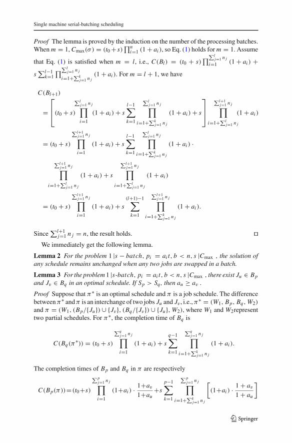
j=1 n j = n, the result holds. ��We immediately get the following lemma.

Lemma 2 For the problem 1 |s − batch, pi = ai t, b < n, s |Cmax , the solution ofany schedule remains unchanged when any two jobs are swapped in a batch.

Lemma 3 For the problem 1 |s-batch, pi = ai t, b < n, s |Cmax , there exist Ju ∈ Bp

and Jv ∈ Bq in an optimal schedule. If Sp > Sq , then au ≥ av .

Proof Suppose that π∗ is an optimal schedule and π is a job schedule. The differencebetween π∗ and π is an interchange of two jobs Ju and Jv , i.e., π∗ = (W1, Bp, Bq , W2)

and π = (W1, (Bp/{Ju}) ∪ {Jv}, (Bq/{Jv}) ∪ {Ju}, W2), where W1 and W2representtwo partial schedules. For π∗, the completion time of Bq is

C(Bq(π∗)) = (t0 + s)

∑qj=1 n j∏

i=1

(1 + ai ) + sq−1∑

k=1

∑qj=1 n j∏

i=1+∑kj=1 n j

(1 + ai ).

The completion times of Bp and Bq in π are respectively

C(Bp(π))=(t0+s)

∑pj=1 n j∏

i=1

(1+ai ) · 1+av

1+au+s

p−1∑

k=1

∑pj=1 n j∏

i=1+∑kj=1 n j

[

(1+ai ) · 1 + av

1 + au

]

123

J. Pei et al.

and C(Bq(π)) = [C p(π) + s] ·∑q

j=1 n j∏

i=1+∑q−1j=1 n j

(1 + ai ) · 1 + au

1 + av

= (t0 + s)

∑qj=1 n j∏

i=1

(1 + ai ) + sq−2∑

k=1

∑qj=1 n j∏

i=1+∑kj=1 n j

(1 + ai )

+ s

∑qj=1 n j∏

i=1+∑q−1j=1 n j

(1 + ai ) · 1 + au

1 + av

.

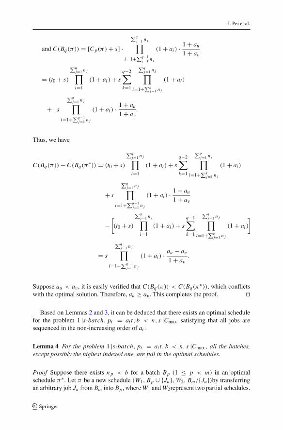
Thus, we have

C(Bq(π)) − C(Bq(π∗)) = (t0 + s)

∑qj=1 n j∏

i=1

(1 + ai ) + sq−2∑

k=1

∑qj=1 n j∏

i=1+∑kj=1 n j

(1 + ai )

+ s

∑qj=1 n j∏

i=1+∑q−1j=1 n j

(1 + ai ) · 1 + au

1 + av

−[

(t0 + s)

∑qj=1 n j∏

i=1

(1 + ai ) + sq−1∑

k=1

∑qj=1 n j∏

i=1+∑kj=1 n j

(1 + ai )

]

= s

∑qj=1 n j∏

i=1+∑q−1j=1 n j

(1 + ai ) · au − av

1 + av

.

Suppose au < av , it is easily verified that C(Bq(π)) < C(Bq(π∗)), which conflictswith the optimal solution. Therefore, au ≥ av . This completes the proof. ��

Based on Lemmas 2 and 3, it can be deduced that there exists an optimal schedulefor the problem 1 |s-batch, pi = ai t, b < n, s |Cmax satisfying that all jobs aresequenced in the non-increasing order of ai .

Lemma 4 For the problem 1 |s-batch, pi = ai t, b < n, s |Cmax , all the batches,except possibly the highest indexed one, are full in the optimal schedules.

Proof Suppose there exists n p < b for a batch Bp (1 ≤ p < m) in an optimalschedule π∗. Let π be a new schedule (W1, Bp ∪ {Ju}, W2, Bm/{Ju})by transferringan arbitrary job Ju from Bm into Bp, where W1 and W2represent two partial schedules.

123

Single machine serial-batching scheduling

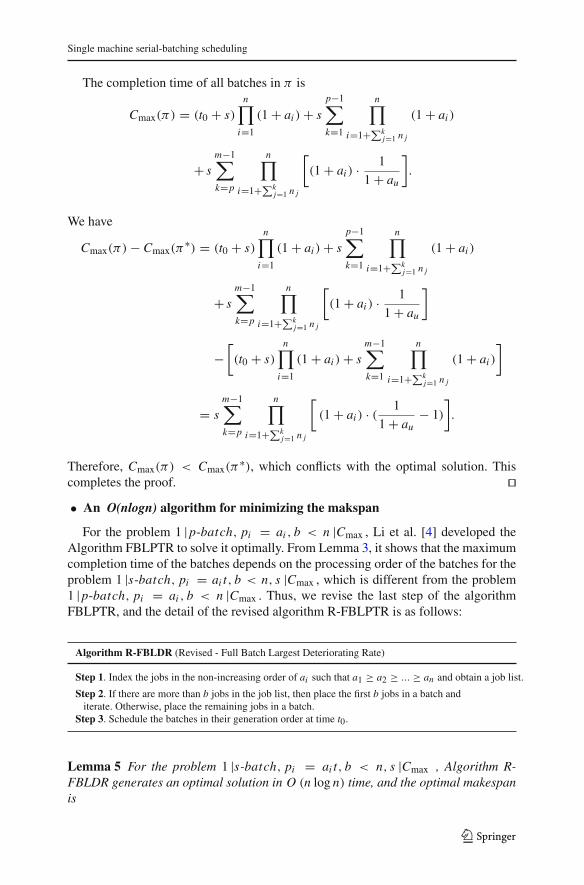
The completion time of all batches in π is

Cmax(π) = (t0 + s)n∏

i=1

(1 + ai ) + sp−1∑

k=1

n∏

i=1+∑kj=1 n j

(1 + ai )

+ sm−1∑

k=p

n∏

i=1+∑kj=1 n j

[

(1 + ai ) · 1

1 + au

]

.

We have

Cmax(π) − Cmax(π∗) = (t0 + s)

n∏

i=1

(1 + ai ) + sp−1∑

k=1

n∏

i=1+∑kj=1 n j

(1 + ai )

+ sm−1∑

k=p

n∏

i=1+∑kj=1 n j

[

(1 + ai ) · 1

1 + au

]

−[

(t0 + s)n∏

i=1

(1 + ai ) + sm−1∑

k=1

n∏

i=1+∑kj=1 n j

(1 + ai )

]

= sm−1∑

k=p

n∏

i=1+∑kj=1 n j

[

(1 + ai ) · (1

1 + au− 1)

]

.

Therefore, Cmax(π) < Cmax(π∗), which conflicts with the optimal solution. This

completes the proof. ��• An O(nlogn) algorithm for minimizing the makspan

For the problem 1 |p-batch, pi = ai , b < n |Cmax , Li et al. [4] developed theAlgorithm FBLPTR to solve it optimally. From Lemma 3, it shows that the maximumcompletion time of the batches depends on the processing order of the batches for theproblem 1 |s-batch, pi = ai t, b < n, s |Cmax , which is different from the problem1 |p-batch, pi = ai , b < n |Cmax . Thus, we revise the last step of the algorithmFBLPTR, and the detail of the revised algorithm R-FBLPTR is as follows:

Algorithm R-FBLDR (Revised - Full Batch Largest Deteriorating Rate)

Step 1. Index the jobs in the non-increasing order of ai such that a1 ≥ a2 ≥ ... ≥ an and obtain a job list.

Step 2. If there are more than b jobs in the job list, then place the first b jobs in a batch anditerate. Otherwise, place the remaining jobs in a batch.

Step 3. Schedule the batches in their generation order at time t0.

Lemma 5 For the problem 1 |s-batch, pi = ai t, b < n, s |Cmax , Algorithm R-FBLDR generates an optimal solution in O (n log n) time, and the optimal makespanis

123

J. Pei et al.

C∗max = (t0 + s)

n∏

i=1

(1 + ai ) + s

nb −1∑

k=1

n∏

i=1+kb

(1 + ai ) (2)

Proof Based on Lemmas 2, 3, and 4, Algorithm R-FBLDR can generate an optimalsolution. Also, the result of the optimal makespan can be obtained as Eq. (2). Thetime complicity of Algorithm R-FBLDR and Algorithm FBLDR proposed in [4] isthe same, which was proved to be O (n log n). Thus, the time complicity of AlgorithmR-FBLDR is also O (n log n). ��Corollary 1 For the problem 1 |s − batch, pi = ai t, b < n, s| Lmax, an optimalschedule can be obtained by Algorithm R-FBLDR.

Proof We have

Lmax = maxi=1,2,··· ,n{0, Ci − d} = max{0, Cmax − d}.

If Cmax is minimized, then the maximum lateness is also minimized since d is aconstant. From Lemma 5, the problem 1 |s-batch, pi = ai t, b < n, s |Cmax can besolved optimally by Algorithm R-FBLDR. This completes the proof. ��

3.2 Minimization of the number of tardy jobs

In this subsection, an O(n2) time algorithm is presented for minimizing the numberof tardy jobs. Let X and Y denote the sets of jobs of which the completion times areno more than and more than the common due date d, respectively. We first give someuseful lemmas for the optimal solutions.

Lemma 6 For the problem 1 |s-batch, pi = ai t, b < n, s| ∑ Ui , the optimal sched-ule satisfies the property that the job sequence in each batch can be in any order.

Lemma 7 For the problem 1 |s-batch, pi = ai t, b < n, s| ∑ Ui , there exists an opti-mal schedule satisfying the following properties:

(1) If the number of batches in X is no less than 2, then all the batches are full exceptpossibly the highest indexed batch in X.

(2) If there exists a batch bk in Y satisfying that S(Bk) < d and C(Bk) > d, then(S(Bk) + s)(1 + ai ) > d(Ji ∈ Y ).

(3) The jobs in X are sequenced in non-increasing order of ai .(4) The deterioration rate of an arbitrary job in X is no more than that of other jobs

in Y .

Proof (1) We omit the proof as it is similar to the proof of Lemma 4.(2) If there exists a batch bk in Y satisfying that S(Bk) < d, C(Bk) > d, and

(S(Bk) + s)(1 + ai ) ≤ d(Ji ∈ Y ), then job Ji can be placed into a single batch.The solution can be improved and it contradicts with the optimal schedule. Hence,it can be deduced that (S(Bk) + s)(1 + ai ) > d(Ji ∈ Y ).

123

Single machine serial-batching scheduling

(3) Based on Lemmas 3 and 6, this property can be derived.(4) Suppose that π∗ is an optimal schedule and π is a job schedule. The dif-

ference between π∗ and π is an interchange of two jobs Ju and Jv , i.e.,π∗ = (W1, Bp, W2, Bq , W3) and π = (W1, (Bp/{Ju}) ∪ {Jv}, W2, (Bq/{Jv}) ∪{Ju}, W3), where Bp ⊆ X , Bp ⊆ Y , and W1, W2, and W3 represent a partialschedule, respectively. The completion time of Bp in π∗ is

C(Bp(π∗)) = (t0 + s)

∑pj=1 n j∏

i=1

(1 + ai ) + sp−1∑

k=1

∑pj=1 n j∏

i=1+∑kj=1 n j

(1 + ai ).

The completion time of Bp in π is

C(Bp(π)) = (t0 + s)

∑pj=1 n j∏

i=1

(1+ai ) · 1+av

1+au+ s

p−1∑

k=1

∑pj=1 n j∏

i=1+∑kj=1 n j

[

(1+ai ) · 1 + av

1 + au

]

.

We have

C(Bp(π∗)) − C(Bp(π)) = (t0 + s)

∑pj=1 n j∏

i=1

(1 + ai ) · au − av

1 + au

+ sp−1∑

k=1

∑pj=1 n j∏

i=1+∑kj=1 n j

[

(1 + ai ) · au − av

1 + au

]

.

If au > av , then it is easily verified that C(Bp(π)) < C(Bp(π∗)), which conflicts

with the optimal solution. Therefore, au ≤ av . This completes the proof. ��• An O(n2) algorithm for minimizing the total number of tardy jobs

Based on the above lemmas, we design the following Algorithm 2 to solve theproblem 1 |s-batch, pi = ai t, b < n, s| ∑ Ui .

Algorithm 2

Step 1. Index the jobs such that a1 ≥ a2 ≥ ... ≥ an and obtain a job list.

Step 2. Set f = 1, T = 0.

Step 3. Initialize the batches, and set σ = φ, k = 1, i = f , bk = {Ji }, nk = 1, and T = (t0 + s)(1 + a f ).

Step 4. If i < n, then update i = i + 1 and go to step 5. Otherwise, batch the remaining jobsarbitrarily and output the schedule σ .

Step 5. If nk < b, then update bk = bk ∪ {Ji }, nk = nk + 1, and T = T · (1 + ai ). Otherwise,update σ = σ ∪ bk , k = k + 1, bk = {Ji }, nk = 1, and T = (T + s)(1 + ai ).

Step 6. If T ≤ d, then go to step 4. Otherwise, update f = f + 1 and go to step 3.

123

J. Pei et al.

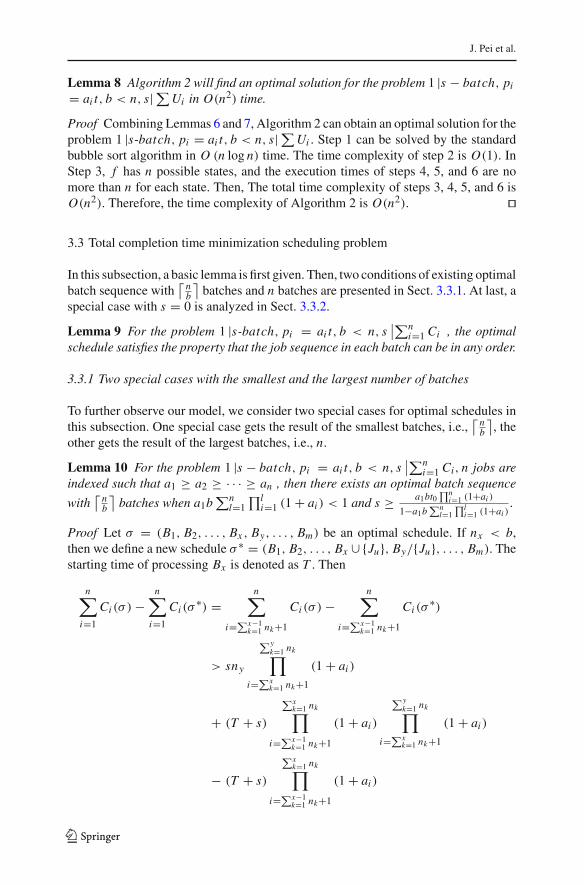
Lemma 8 Algorithm 2 will find an optimal solution for the problem 1 |s − batch, pi

= ai t, b < n, s| ∑ Ui in O(n2) time.

Proof Combining Lemmas 6 and 7, Algorithm 2 can obtain an optimal solution for theproblem 1 |s-batch, pi = ai t, b < n, s| ∑ Ui . Step 1 can be solved by the standardbubble sort algorithm in O (n log n) time. The time complexity of step 2 is O(1). InStep 3, f has n possible states, and the execution times of steps 4, 5, and 6 are nomore than n for each state. Then, The total time complexity of steps 3, 4, 5, and 6 isO(n2). Therefore, the time complexity of Algorithm 2 is O(n2). ��

3.3 Total completion time minimization scheduling problem

In this subsection, a basic lemma is first given. Then, two conditions of existing optimalbatch sequence with

⌈ nb

⌉batches and n batches are presented in Sect. 3.3.1. At last, a

special case with s = 0 is analyzed in Sect. 3.3.2.

Lemma 9 For the problem 1 |s-batch, pi = ai t, b < n, s∣∣∑n

i=1 Ci , the optimalschedule satisfies the property that the job sequence in each batch can be in any order.

3.3.1 Two special cases with the smallest and the largest number of batches

To further observe our model, we consider two special cases for optimal schedules inthis subsection. One special case gets the result of the smallest batches, i.e.,

⌈ nb

⌉, the

other gets the result of the largest batches, i.e., n.

Lemma 10 For the problem 1 |s − batch, pi = ai t, b < n, s∣∣∑n

i=1 Ci, n jobs areindexed such that a1 ≥ a2 ≥ · · · ≥ an , then there exists an optimal batch sequence

with⌈ n

b

⌉batches when a1b

∑nl=1

∏li=1 (1 + ai ) < 1 and s ≥ a1bt0

∏ni=1 (1+ai )

1−a1b∑n

l=1∏l

i=1 (1+ai ).

Proof Let σ = (B1, B2, . . . , Bx , By, . . . , Bm) be an optimal schedule. If nx < b,then we define a new schedule σ ∗ = (B1, B2, . . . , Bx ∪ {Ju}, By/{Ju}, . . . , Bm). Thestarting time of processing Bx is denoted as T . Then

n∑

i=1

Ci (σ ) −n∑

i=1

Ci (σ∗) =

n∑

i=∑x−1k=1 nk+1

Ci (σ ) −n∑

i=∑x−1k=1 nk+1

Ci (σ∗)

> sny

∑yk=1 nk∏

i=∑xk=1 nk+1

(1 + ai )

+ (T + s)

∑xk=1 nk∏

i=∑x−1k=1 nk+1

(1 + ai )

∑yk=1 nk∏

i=∑xk=1 nk+1

(1 + ai )

− (T + s)

∑xk=1 nk∏

i=∑x−1k=1 nk+1

(1 + ai )

123

Single machine serial-batching scheduling

− (T + s)au(nx + 1)

∑xk=1 nk∏

i=∑x−1k=1 nk+1

(1 + ai ) − s(ny − 1)

· 1

1 + au·

∑yk=1 nk∏

i=∑xk=1 nk+1

(1 + ai )

> s − (T + s)au(nx + 1)

∑xk=1 nk∏

i=∑x−1k=1 nk+1

(1 + ai )

≥ s − a1b

[

t0

n∏

i=1

(1 + ai ) + sn∑

l=1

l∏

i=1

(1 + ai )

]

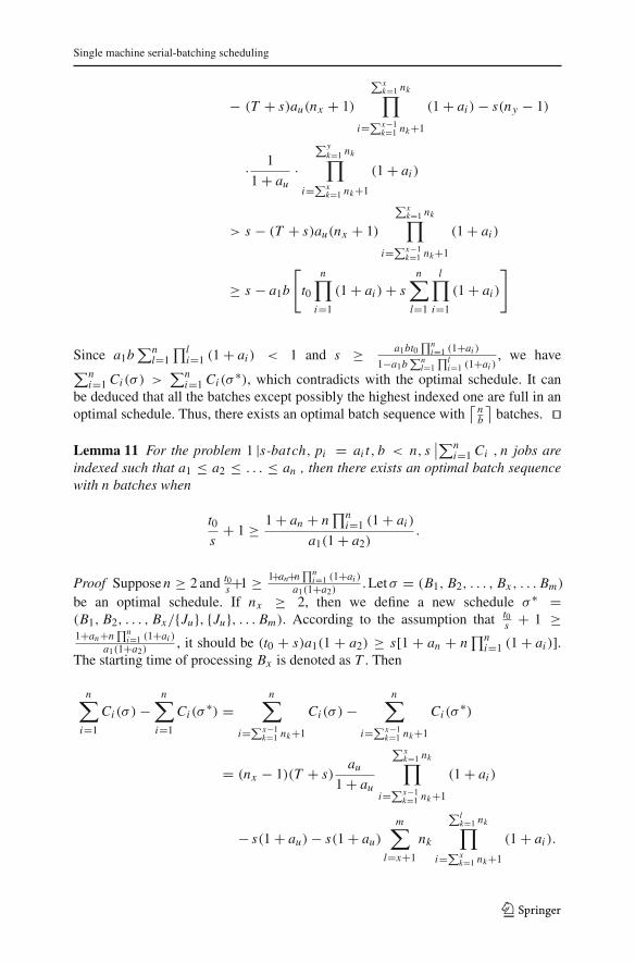
Since a1b∑n

l=1∏l

i=1 (1 + ai ) < 1 and s ≥ a1bt0∏n

i=1 (1+ai )

1−a1b∑n

l=1∏l

i=1 (1+ai ), we have

∑ni=1 Ci (σ ) >

∑ni=1 Ci (σ

∗), which contradicts with the optimal schedule. It canbe deduced that all the batches except possibly the highest indexed one are full in anoptimal schedule. Thus, there exists an optimal batch sequence with

⌈ nb

⌉batches. ��

Lemma 11 For the problem 1 |s-batch, pi = ai t, b < n, s∣∣∑n

i=1 Ci , n jobs areindexed such that a1 ≤ a2 ≤ . . . ≤ an , then there exists an optimal batch sequencewith n batches when

t0s

+ 1 ≥ 1 + an + n∏n

i=1 (1 + ai )

a1(1 + a2).

Proof Suppose n ≥ 2 and t0s+1 ≥ 1+an+n

∏ni=1 (1+ai )

a1(1+a2). Letσ = (B1, B2, . . . , Bx , . . . Bm)

be an optimal schedule. If nx ≥ 2, then we define a new schedule σ ∗ =(B1, B2, . . . , Bx/{Ju}, {Ju}, . . . Bm). According to the assumption that t0

s + 1 ≥1+an+n

∏ni=1 (1+ai )

a1(1+a2), it should be (t0 + s)a1(1 + a2) ≥ s[1 + an + n

∏ni=1 (1 + ai )].

The starting time of processing Bx is denoted as T . Then

n∑

i=1

Ci (σ ) −n∑

i=1

Ci (σ∗) =

n∑

i=∑x−1k=1 nk+1

Ci (σ ) −n∑

i=∑x−1k=1 nk+1

Ci (σ∗)

= (nx − 1)(T + s)au

1 + au

∑xk=1 nk∏

i=∑x−1k=1 nk+1

(1 + ai )

− s(1 + au) − s(1 + au)

m∑

l=x+1

nk

∑lk=1 nk∏

i=∑xk=1 nk+1

(1 + ai ).

123

J. Pei et al.

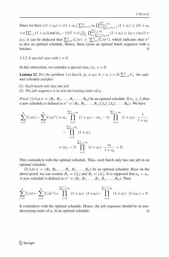
Since we have s(1 + au) + s(1 + au)∑m

l=x+1 nk∏∑l

k=1 nk

i=∑xk=1 nk+1

(1 + ai ) ≤ s[1 + an

+n∏n

i=1 (1 + ai )] and (nx −1)(T +s) au1+au

∏∑xk=1 nk

i=∑x−1k=1 nk+1

(1 + ai ) ≥ (t0 +s)a1(1+a2), it can be deduced that

∑ni=1 Ci (σ ) ≥ ∑n

i=1 Ci (σ∗), which indicates that σ ∗

is also an optimal schedule. Hence, there exists an optimal batch sequence with nbatches. ��

3.3.2 A special case with s = 0

In this subsection, we consider a special case, i.e., s = 0.

Lemma 12 For the problem 1 |s-batch, pi = ai t, b < n, s = 0| ∑ni=1 Ci , the opti-

mal schedule satisfies:

(1) Each batch only has one job.(2) The job sequence is in non-decreasing order of ai .

Proof (1) Let σ = (B1, B2, . . . , Bx , . . . , Bm) be an optimal schedule. If nx ≥ 2, thena new schedule is defined as σ ∗ = (B1, B2, . . . , Bx/{Ju}, {Ju}, . . . , Bm). We have

n∑

i=1

Ci (σ ) −n∑

i=1

Ci (σ∗) = nx

∑xk=1 nk∏

i=1

(1 + ai ) − (nx − 1)

∑xk=1 nk∏

i=1

(1 + ai ) · 1

1 + au

−∑x

k=1 nk∏

i=1

(1 + ai )

= (nx − 1)

∑xk=1 nk∏

i=1

(1 + ai ) · au

1 + au> 0.

This contradicts with the optimal schedule. Thus, each batch only has one job in anoptimal schedule.

(2) Let σ = (B1, B2, . . . , Bx , By, . . . , Bm) be an optimal schedule. Base on theabove proof, we can assume Bx = {Ju} and By = {Jv}. It is supposed that au > av .A new schedule is defined as σ ∗ = (B1, B2, . . . , By, Bx , . . . , Bm). Then

n∑

i=1

Ci (σ )−n∑

i=1

Ci (σ∗)=

∑x−1k=1 nk∏

i=1

(1 + ai ) · (1+au)−∑x−1

k=1 nk∏

i=1

(1 + ai ) · (1+av) > 0.

It contradicts with the optimal schedule. Hence, the job sequence should be in non-decreasing order of ai in an optimal schedule. ��

123

Single machine serial-batching scheduling

• An O(nlogn)algorithm for the special case with s=0

Algorithm 3

Step 1. Index the jobs such that a1 ≤ a2 ≤ . . . ≤ an and obtain a job list.

Step 2. Place each job into a single batch as the job sequence.

Step 3. Schedule the batches in their generation order at time t0.

Lemma 13 For the problem 1 |s-batch, pi = ai t, b < n, s = 0| ∑ni=1 Ci , Algorithm

3 generates the optimal solution in O (n log n) time, and the minimum total completiontime is

n∑

i=1

Ci = t0

n∑

l=1

l∏

i=1

(1 + ai ) (3)

Proof Based on Lemma 12, Algorithm 3 can generate the optimal solution for theproposed problem, and the result of the minimum total completion time is as Eq. (3)shows. Step 1 can be solved by the standard bubble sort algorithm in O (n log n) time,and the total time complexity of steps 2 and 3 is O (n). Therefore, the time complexityof Algorithm 3 is O (n log n). ��

4 Conclusion

In this paper, we have considered the single serial-batching machine scheduling prob-lems with independent setup time and deteriorating jobs. Job processing times aredescribed by a linear function of time. We propose optimization algorithms for theproblems of minimizing the makespan and the total number of tardy jobs, respectively.In addition, for the problem of minimizing the total completion time, two special caseswith the smallest and the largest number of batches are studied, and an optimal algo-rithm is presented for the special case with s = 0.

Acknowledgments We would like to thank the editors and referees for their valuable comments andsuggestions. This work is supported by the National Natural Science Foundation of China (Nos. 71231004,71171071, 71131002), and LATNA laboratory, NRU HSE, RF government grant, ag. 11.G34.31.0057.

References

1. Gupta, J.N.D., Gupta, S.K.: Single facility scheduling with nonlinear processing times. Comput. Ind.Eng. 14, 387–393 (1988)

2. Browne, S., Yechiali, U.: Scheduling deteriorating jobs on a single processor. Oper. Res. 38, 495–498(1990)

3. Qi, X.L., Zhou, S.G., Yuan, J.J.: Single machine parallel-batch scheduling with deteriorating jobs.Theor. Comput. Sci. 410, 830–836 (2009)

4. Li, S.S., Ng, C.T., Cheng, T.C.E., Yuan, J.J.: Parallel-batch scheduling of deteriorating jobs with releasedates to minimize the makespan. Eur. J. Oper. Res. 210, 482–488 (2011)

123

J. Pei et al.

5. Miao, C.X., Zhang, Y.Z., Cao, Z.G.: Bounded parallel-batch scheduling on single and multi machinesfor deteriorating jobs. Inf. Process. Lett. 111, 798–803 (2011)

6. Miao, C.X., Zhang, Y.Z., Wu, C.L.: Scheduling of deteriorating jobs with release dates to minimizethe maximum lateness. Theor. Comput. Sci. 462, 80–87 (2012)

7. Wu, C.C., Shiau, Y.R., Lee, W.C.: Single-machine group scheduling problems with deterioration con-sideration. Comput. Oper. Res. 35, 1652–1659 (2008)

8. Wu, C.C., Lee, W.C.: Single-machine group-scheduling problems with deteriorating setup times andjob-processing times. Int. J. Prod. Econ. 115, 128–133 (2008)

9. Wang, J.B., Lin, L., Shan, F.: Single-machine group scheduling problems with deteriorating jobs. Int.J. Adv. Manuf. Technol. 39, 808–812 (2008)

10. Wang, J.B., Gao, W.J., Wang, L.Y., Wang, D.: Single machine group scheduling with general lineardeterioration to minimize the makespan. Int. J. Adv. Manuf. Technol. 43, 146–150 (2009)

11. Zhang, X.G., Yan, G.L.: Single-machine group scheduling problems with deteriorated and learningeffect. Appl. Math. Comput. 216, 1259–1266 (2010)

12. Yang, S.J., Yang, D.L.: Single-machine group scheduling problems under the effects of deteriorationand learning. Comput. Ind. Eng. 58, 754–758 (2010)

13. Wang, J.B., Sun, L.Y.: Single-machine group scheduling with linearly decreasing time-dependent setuptimes and job processing times. Int. J. Adv. Manuf. Technol. 49, 765–772 (2010)

14. Wei, C.M., Wang, J.B.: Single machine quadratic penalty function scheduling with deteriorating jobsand group technology. Appl. Math. Model. 34, 3642–3647 (2010)

15. Huang, X., Wang, M.Z., Wang, J.B.: Single-machine group scheduling with both learning effects anddeteriorating jobs. Comput. Ind. Eng. 60, 750–754 (2011)

16. Yang, S.J.: Group scheduling problems with simultaneous considerations of learning and deteriorationeffects on a single-machine. Appl. Math. Model. 35, 4008–4016 (2011)

17. Bai, J., Li, Z.R., Huang, X.: Single-machine group scheduling with general deterioration and learningeffects. Appl. Math. Model. 36, 1267–1274 (2012)

18. Lee, W.C., Lu, Z.S.: Group scheduling with deteriorating jobs to minimize the total weighted numberof late jobs. Appl. Math. Comput. 218, 8750–8757 (2012)

19. Wang, J.B., Huang, X., Wu, Y.B., Ji, P.: Group scheduling with independent setup times, ready times,and deteriorating job processing times. Int. J. Adv. Manuf. Technol. 60, 643–649 (2012)

20. Wang, D., Huo, Y.Z., Ji, P.: Single-machine group scheduling with deteriorating jobs and allottedresource. Optim. Lett. (2012). doi:10.1007/s11590-012-0577-2

21. Xuan, H., Tang, L.X.: Scheduling a hybrid flowshop with batch production at the last stage. Comput.Oper. Res. 34, 2718–2733 (2007)

22. Graham, R.L., Lawler, E.L., Lenstra, J.K., Rinnooy Kan, A.H.G.: Optimization and approximation indeterministic sequencing and scheduling: a survey. Ann. Discret. Math. 5, 287–326 (1979)

123