Embed Size (px)
Citation preview
Slip Control during Slope Descent for a Rover with
Plowing Capability
Daniel Loret de Mola Lemus
CMU-RI-TR-13-10
Submitted in partial fulfillment of the
requirements for the degree of
Masters of Science in Robotics
The Robotics Institute
Carnegie Mellon University
Pittsburgh, Pennsylvania 15213
May 2013
Masters Committee:
David Wettergreen, Chair
William “Red” Whittaker
Scott Moreland
Copyright © 2013 by Daniel Loret de Mola Lemus. All rights reserved.

i
Abstract
Recent efforts in planetary robotic exploration aim toward craters, skylights, and other
depressions with challenging terrain conditions. The access to such places requires traversing on
extreme slopes where high levels of slip greatly hamper rover mobility and control. To
successfully reach valuable targets such as water ice and mineral outcrops in these locations, slip
must be promptly arrested. The work presented here develops an automatic system for a
plowing-capable rover that controls slip during descent on steep unconsolidated slopes.
The slip control system is implemented around the robot’s plow, and has two main
components: a slip estimation subsystem and the slip controller. Slip estimation is performed
through a visual odometry algorithm based on monocular optical flow. Two approaches were
explored for the slip controller: PID and fuzzy logic control. The design of the controllers was
aided by a model of the rover-terrain system formulated specifically for this purpose.
Field testing was carried out on conditions relevant to lunar crater exploration. The
experimental results showed that the control system is able to keep slip to a minimum for
different commanded vehicle speeds and slopes as steep as 31°. As a consequence, this work
expands current rover mobility and control capabilities by enabling precise descent on steep
slopes of unconsolidated material.

ii
Dedication
To my mother, whose tireless efforts and perseverance have
opened invaluable opportunities in my life.
To my father, whose professional excellence inspires all my
endeavors.
iii
Acknowledgements
I would like to thank my advisor, David Wettergreen, for his experienced guidance and constant
support throughout the development of this work and, in general, during my time in the Robotics
Institute. I am taking with me lessons that go beyond the academic setting.
I would also like to thank my former professor, Aarón Sariñana, for being amazingly
generous with his time and for his insightful advice on controls. I am grateful that he has kept
sharing with me his knowledge and expertise after I graduated from college.
I extend my gratitude to the planetary robotics group led by David Wettergreen, especially
Scott Moreland, Chuck Whittaker, and David Kohanbash. Scott was always available to answer
my never ending questions on terramechanics. Chuck’s assistance during field testing was
incredible, and he also gave Icebreaker another breath of life to complete the final experiments.
David Kohanbash was very helpful in troubleshooting several quirks of Icebreaker.
Finally, I would also like to thank Colin Creager and Kyle Johnson from NASA Glenn
Research Center for their wide support and ample time flexibility during field testing.
iv
Contents
List of Figures ................................................................................................................................ vi
List of Tables ................................................................................................................................. ix
1 Introduction...............................................................................................................................1
1.1 Related Work .................................................................................................................. 2
1.1.1 Dynamic modeling.................................................................................................. 2
1.1.2 Slip estimation ........................................................................................................ 3
1.1.3 Slip compensation/control strategies ...................................................................... 3
1.2 Problem Statement .......................................................................................................... 4
1.3 Overview of the Control System..................................................................................... 7
1.4 Overview of Thesis ......................................................................................................... 8
2 Dynamics of Rover-Terrain Interactions ..................................................................................9
2.1 Background on Terramechanics of a Track .................................................................... 9
2.2 Rover’s Model .............................................................................................................. 12
2.2.1 Kinematic model................................................................................................... 13
2.2.2 Dynamic model..................................................................................................... 14
2.3 Parameter Identification................................................................................................ 15
2.3.1 Experiment design ................................................................................................ 16
2.3.2 Planar terrain case ................................................................................................. 18
2.3.3 Inclined terrain case .............................................................................................. 21
3 Vision System.........................................................................................................................26
3.1 Background on Visual Odometry ................................................................................. 27
3.2 Algorithm Description .................................................................................................. 28
3.3 Performance on Lunar Regolith.................................................................................... 38
v
4 Classical Controllers...............................................................................................................42
4.1 Performance Objectives ................................................................................................ 43
4.2 On-Off Controller ......................................................................................................... 43
4.2.1 Design ................................................................................................................... 43
4.3 PI Controller.................................................................................................................. 44
4.3.1 Design ................................................................................................................... 44
4.3.2 Simulations ........................................................................................................... 45
5 Fuzzy Logic Controller...........................................................................................................50
5.1 Background on Fuzzy Logic......................................................................................... 50
5.1.1 Fundamental Theory ............................................................................................. 51
5.1.2 Fuzzy Logic Control ............................................................................................. 58
5.2 Design ........................................................................................................................... 60
5.3 Simulations ................................................................................................................... 65
6 Experimental Results ..............................................................................................................70
6.1 Experiment Design........................................................................................................ 71
6.2 Descent without Slip Control........................................................................................ 72
6.3 Slip-Control Proof of Concept: On-Off Controller....................................................... 74
6.4 Slip Regulation.............................................................................................................. 76
6.5 Nonzero Slip Reference ................................................................................................ 85
6.6 Slip Control with Odometric Error ............................................................................... 88
7 Discussion...............................................................................................................................92
7.1 Conclusions................................................................................................................... 92
7.2 Summary of Contributions............................................................................................ 93
7.3 Future Research ............................................................................................................ 94
References......................................................................................................................................96
vi
List of Figures
Fig. 1.1 Icebreaker rover ................................................................................................................ 5
Fig. 1.2 Diagram block representation of slip control system ....................................................... 7
Fig. 2.1 Tractive effort of a track................................................................................................. 10
Fig. 2.2 Skid-steering of the robot ............................................................................................... 13
Fig. 2.3 Free body diagram of the robot ...................................................................................... 14
Fig. 2.4 NASA GRC SLOPE facility........................................................................................... 17
Fig. 2.5 Model’s outputs for driving curves on horizontal terrain............................................... 19
Fig. 2.6 Model’s outputs for driving a straight line ..................................................................... 20
Fig. 2.7 Model’s output for descending without plow................................................................. 21
Fig. 2.8 Model’s output for descending with 0.07 m plow depth................................................ 22
Fig. 2.9 Model’s output for descending with 0.14 m plow depth. ............................................... 23
Fig. 2.10 Model’s output for descending with 0.20 m plow depth. ............................................. 23
Fig. 2.11 Model validation for descending with 0.035 m plow depth ......................................... 24
Fig. 2.12 Model validation for descending with 0.07 m plow depth ........................................... 25
Fig. 2.13 Model validation for descending with 0.10 m plow depth. .......................................... 25
Fig. 3.1 Vision system’s camera .................................................................................................. 26
Fig. 3.2 Flow chart diagram of the visual odometry algorithm. .................................................. 29
Fig. 3.3 Creation of feature selection mask ................................................................................. 31
Fig. 3.4 Image feature selection................................................................................................... 32
Fig. 3.5 Vision system’s speed estimation without plow.............................................................. 39
Fig. 3.6 Vision system’s speed estimation with 0.17 m plow depth............................................ 40
Fig. 3.7 Vision system’s speed estimation with 0.14 m plow depth............................................ 40
Fig. 3.8 Vision system’s speed estimation with 0.20 m plow depth............................................. 41
Fig. 4.1 Block diagram of PI control system ............................................................................... 45
Fig. 4.2 Simulation of PI controller regulating slip ..................................................................... 46
Fig. 4.3 Simulation of PI controller rejecting a disturbance ........................................................ 47
vii
Fig. 4.4 Simulation of PI controller under step change in reference ........................................... 48
Fig. 4.5 Simulation of PI controller in the presence of noise ...................................................... 49
Fig. 5.1 Membership function of a fuzzy set ............................................................................... 51
Fig. 5.2 Clipping inference method ............................................................................................. 54
Fig. 5.3 Scaling inference method ............................................................................................... 54
Fig. 5.4 Superimposition of inferred conclusions........................................................................ 54
Fig. 5.5 Fuzzy rule-based inference............................................................................................. 56
Fig. 5.6 Fuzzy control architecture .............................................................................................. 58
Fig. 5.7 Block diagram of fuzzy logic control system................................................................. 61
Fig. 5.8 Membership functions of error signal ............................................................................ 62
Fig. 5.9 Membership functions of change in error signal ............................................................ 63
Fig. 5.10 Membership functions of change in process’ input signal ........................................... 63
Fig. 5.11 Control surface ............................................................................................................. 65
Fig. 5.12 Simulation of fuzzy controller regulating slip.............................................................. 66
Fig. 5.13 Simulation of fuzzy controller rejecting a disturbance................................................. 67
Fig. 5.14 Simulation of fuzzy controller under step change in reference .................................... 68
Fig. 5.15 Simulation of fuzzy controller in the presence of noise ............................................... 69
Fig. 6.1 NASA GRC Dunes testing site....................................................................................... 71
Fig. 6.2 Descent at 0.3 rad/s without slip control ........................................................................ 73
Fig. 6.3 Descent at 0.42 rad/s without slip control ...................................................................... 73
Fig. 6.4 Experiment of on-off slip controller ............................................................................... 75
Fig. 6.5 Experiment of FLC regulating slip on 31° slope at 0.3 rad/s ......................................... 77
Fig. 6.6 Experiment of PI regulating slip on 31° slope at 0.3 rad/s ............................................. 78
Fig. 6.7 Experiment of FLC regulating slip on 31° slope at 0.4 rad/s ......................................... 79
Fig. 6.8 Experiment of PI regulating slip on 31° slope at 0.4 rad/s ............................................. 80
Fig. 6.9 Experiment of FLC regulating slip on 25° slope at 0.4 rad/s ......................................... 81
Fig. 6.10 Experiment of PI regulating slip on 25° at 0.4 rad/s .................................................... 82
Fig. 6.11 Experiment of FLC regulating slip on 20° slope at 0.2 rad/s ....................................... 83
Fig. 6.12 Experiment of PI regulating slip on 20° slope at 0.2 rad/s ........................................... 84
Fig. 6.13 Nonzero slip reference experiment with FLC .............................................................. 86

viii
Fig. 6.14 Nonzero slip reference experiment with PI ................................................................... 87
Fig. 6.15 Experiment of FLC regulating slip on not locally planar terrain ................................. 89
Fig. 6.16 Experiment of FLC in Dunes........................................................................................ 90
Fig. 6.17 Experiment of PI in Dunes ........................................................................................... 91

ix
List of Tables
Table 2.1 Vehicle parameters ...................................................................................................... 16
Table 2.2 Soil parameters of GRC-1............................................................................................ 17
Table 3.1 Camera’s technical specifications................................................................................ 27
Table 5.1 Rule-base of FLC......................................................................................................... 64
1
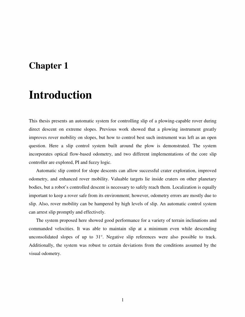
Chapter 1
Introduction
This thesis presents an automatic system for controlling slip of a plowing-capable rover during
direct descent on extreme slopes. Previous work showed that a plowing instrument greatly
improves rover mobility on slopes, but how to control best such instrument was left as an open
question. Here a slip control system built around the plow is demonstrated. The system
incorporates optical flow-based odometry, and two different implementations of the core slip
controller are explored, PI and fuzzy logic.
Automatic slip control for slope descents can allow successful crater exploration, improved
odometry, and enhanced rover mobility. Valuable targets lie inside craters on other planetary
bodies, but a robot’s controlled descent is necessary to safely reach them. Localization is equally
important to keep a rover safe from its environment; however, odometry errors are mostly due to
slip. Also, rover mobility can be hampered by high levels of slip. An automatic control system
can arrest slip promptly and effectively.
The system proposed here showed good performance for a variety of terrain inclinations and
commanded velocities. It was able to maintain slip at a minimum even while descending
unconsolidated slopes of up to 31°. Negative slip references were also possible to track.
Additionally, the system was robust to certain deviations from the conditions assumed by the
visual odometry.
1 Introduction
2
1.1 Related Work
Research on slope descent of rovers is in an early stage. Ziglar [1] and Kohanbash [2]
demonstrated that a plowing-capable tracked rover can successfully descend severe slopes with
low slippage. However, in a planetary mission a rover must have the capability to control slip
autonomously. Since research on dedicated slip control systems for robotic vehicles has been
scarce, the next subsections will present current work on the three necessary elements of a slip
control system: dynamic modeling, slip estimation, and slip compensation/control strategies.
1.1.1 Dynamic modeling
A rover’s vehicle-terrain interaction model is useful for analysis, simulation, and control. Models
of tracked vehicles have been proposed in terramechanics standard literature. But these do not
focus on slope traversal. More recently, some models have been proposed for slope traversal of
wheeled rovers.
Dynamic models of tracked vehicles on level terrain can be found in the standard
terramechanics literature. One example is J. Y. Wong’s model of a vehicle with rigid tracks [3].
Based on previous work by Bekker [4], he proposed a simple model that describes the steering of
a tracked vehicle on level ground and that is applicable to different types of soil. A more
complex model was devised by Muro and O’Brien [5]. This one uses a more realistic pressure
distribution under the track which takes into account center of mass displacement around the
track’s midline. The model requires several numerical procedures to solve for forces and slip.
With the recent interest on exploration of craters in other planetary bodies, some models that
deal with slope traversal have arisen. They are modifications of the classical wheel-soil
interaction models. One example is Ishigami et al.’s wheel model on inclined surface [6]. It takes
into account lateral forces due to wheel sinkage, and was used to analyze slope climbing and
cross-traversing capabilities of a rover. A similar approach was taken by Huang et al. [7]. In his
model, sinkages of the front and rear wheels are calculated separately, and was used to simulate
down-slope travel of a lunar rover.
Dynamic models of tracked vehicles have been proposed in the past, but they deal with level
terrain. Recent studies are starting to deal with slopes. The resulting models are adaptations of
the classical wheel-soil interaction model.
1 Introduction
3
1.1.2 Slip estimation
In order for a rover to automatically control its slip, it must have the capability to perceive and
estimate the degree of such phenomenon. The approaches to estimate slip can be grouped into
three broad groups: current-based, visual odometry, and indirect sensor fusion.
In current-based methods, motor currents of the running gear are mapped to slip by relating
current to torque, and torque to slip. This method was demonstrated by Ojeda et al. to correct
odometry of a six-wheeled Mars-analogous rover [8]. The technique requires knowledge of the
terrain. To gather such knowledge, two types of procedures are proposed. The first one requires
positional ground truth. The second one can only be applied to platforms with four or more
independently driven wheels.
Another method that has been used to detect slip is visual odometry. One instance is the
stereo feature tracking system implemented in the Mars Exploration Rovers (MER) [9]. When
the system was used, it detected slip and corrected position estimates accordingly. A faster and
more reliable version of this algorithm was programmed in the Mars Science Laboratory rover
(MSL) [10]. A monocular optical flow alternative was presented by Seegmiller and Wettergeen
[11]. Their method focused on reducing wrong measurements due to the effects of the rover’s
shadow in the images.
The third type of method consists in refining slip predictions from a vehicle’s model with
sensor measurements. The model can be kinematic or dynamic, but researchers frequently use
the latter. Le et al., for example, proposed an extended Kalman filter (EKF) that used position
measurements to compute the slip parameters of a tracked vehicle [12]. Dar and Longoria
applied this idea to a small tracked vehicle driving on flat terrain [13].
The methods to estimate slip are diverse in nature, but, given current research on the topic,
they can be classified into motor-current-based, visual odometry-based, and indirect sensor
fusion-based.
1.1.3 Slip compensation/control strategies
Currently, slip control has mostly been done in the form of compensation rather than direct
control. Hence, there are very few instances in which slip has been formalized as a control
problem.
1 Introduction
4
In a compensation approach some measure is taken to keep slip within an acceptable range.
The compensator is usually an additional component of a greater control scheme such as path
tracking. One example is the autonomous tracked excavator presented in [14]. Its slip
compensator decreases commanded track velocities by a constant factor when slip is greater than
a fixed threshold. A slightly more deliberate approach is taken by Ishigami et al. in [15]. His
compensator works to enable path tracking of a rover driving on a side slope. In order to keep
longitudinal wheel slip near a reference, each angular wheel speed is modified in proportion to
how far its slip is from the reference.
In direct control, the system would be exclusively dedicated to drive slip to the desired value.
Yoshida and Hamano applied this approach to a six-wheeled rover traversing small ditches on
loose soil [16]. He used a PI controller to regulate motor torques to achieve the desired slip. To
estimate slip, an empirical table relating motor duty cycle to slip was programmed in the robot.
The few slip control examples for robotic vehicles are within the area of compensation. The
cases of direct slip control systems are almost inexistent.
1.2 Problem Statement
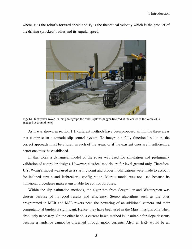
This thesis addresses the problem of developing an automatic system for a plowing-capable
rover to control slip during direct descent on steep unconsolidated slopes. The system is
implemented on the Icebreaker rover, a tracked robot with a plowing instrument (fig. 1.1). The
instrument, here called “plow,” is a one degree of freedom mechanism that can be driven into the
ground to act as a breaking device. The plow improves mobility in slopes of up to 38°. The slip
control system was built around the plow.
The focus is on direct descent and on slopes around 30° covered with unconsolidated
material. Direct descent means a straight traverse down-slope along the steepest direction.
Unconsolidated material refers to loose frictional soil. These two conditions validate the system
under high levels of slide (negative slip) similar to those that would be encountered while
descending a lunar crater.
Slip to be controlled is defined as:
T
T
vehicleV
xVi
&−=
(1.1)
1 Introduction
5
where x& is the robot’s forward speed and VT is the theoretical velocity which is the product of
the driving sprockets’ radius and its angular speed.
Fig. 1.1 Icebreaker rover. In this photograph the robot’s plow (dagger-like rod at the center of the vehicle) is
engaged at ground level.
As it was shown in section 1.1, different methods have been proposed within the three areas
that comprise an automatic slip control system. To integrate a fully functional solution, the
correct approach must be chosen in each of the areas, or if the existent ones are insufficient, a
better one must be established.
In this work a dynamical model of the rover was used for simulation and preliminary
validation of controller designs. However, classical models are for level ground only. Therefore,
J. Y. Wong’s model was used as a starting point and proper modifications were made to account
for inclined terrain and Icebreaker’s configuration. Muro’s model was not used because its
numerical procedures make it unsuitable for control purposes.
Within the slip estimation methods, the algorithm from Seegmiller and Wettergreen was
chosen because of its good results and efficiency. Stereo algorithms such as the ones
programmed in MER and MSL rovers need the powering of an additional camera and their
computational burden is significant. Hence, they have been used in the Mars missions only when
absolutely necessary. On the other hand, a current-based method is unsuitable for slope descents
because a landslide cannot be discerned through motor currents. Also, an EKF would be an
1 Introduction
6
inappropriate method. An EKF requires linearizations not well suited for the complex dynamics
of slope descents.
Finally, a simple compensation control method would not be enough to cope with the slip
phenomena experienced on highly inclined terrain. Landslides can suddenly occur and drag the
robot down-slope. A prompt and effective action must be taken in these cases. A dedicated slip
control system can provide this.
There are three main reasons that demand a rover to be able to autonomously control its slip
while descending extreme slopes: targets inside craters in other planetary bodies, the inadequacy
of controlling slip through teleoperation, and odometry errors.
First, findings of valuable targets inside craters must be confirmed through robotic explorers
capable of maneuvering on steep slopes and loose soil. For instance, NASA’s orbiter found large
deposits of water ice in the moon’s craters [17]. However, these craters have slopes of 30° - 40°
and are covered with fine regolith [18]. Other targets of scientific interest are geological
formations in Mars’ craters which could explain the origin of the planet [19].
The second reason is that a human would not be able to properly control rover’s slip via
teleoperation. During steep descents, sudden landslides under the robot’s running gear can carry
away the rover into potential threats. A fast response is necessary to counteract these
disturbances. Additionally, there is not an obvious way of manually enforcing an adequate slip
control strategy.
The third reason is that most odometry errors are due to slip. This is even more prominent in
rovers because the terrain in places such as the Moon or Mars is covered with fine loose regolith.
Minimizing slip and, as a consequence, odometry errors, would reduce the time and power
required for a rover to reach targets that, for example, could be located on the walls of craters.
In summary, this thesis presents a solution on how to automatically control the slip of a
plowing-capable rover during direct descent on extreme slopes. Current research exists on
dynamic modeling of rovers, slip estimation, and slip compensation. An integration of these
elements is necessary to bestow a rover the ability to safely descend steep slopes. This ability is
of utmost importance given recent discoveries that suggest the existence of valuable resources in
craters on other planetary bodies, the inherent difficulty of manually controlling slip, and the
necessity of more precise odometry.
1 Introduction
7
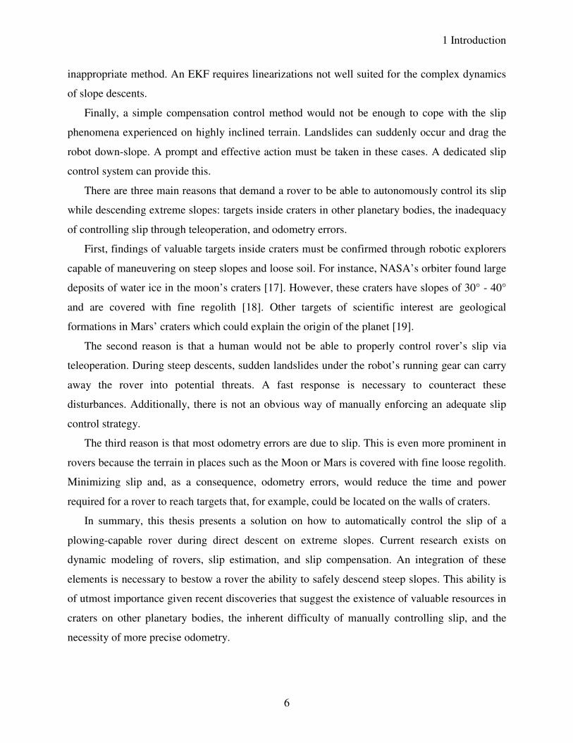
1.3 Overview of the Control System
The purpose of the system is to control slip as defined in eq. (1.1) by actuating the robot’s plow.
The angular speeds of the driving sprockets are not modified by the system. At the top level the
desired slip value is selected. The control system’s components are the plant, the controller, the
sensor, and the signals. A block diagram representation is shown in fig. 1.2.
Fig. 1.2 Diagram block representation of slip control system. The flow of information in the system is
represented by the arrows.
The plant is the vehicle-terrain system. The input to the plant is plow depth. The output of the
plant is the robot’s forward velocity. The sensor estimates this velocity, compares it with the
driving sprockets’ encoder data, and computes slip. The sensor is comprised by the camera,
visual odometry algorithm, and the application of equation (1.1). The plant and sensor together
form the process. The controller’s input is the error signal computed as the difference between
the set point and the estimated slip. The controller’s output is the commanded plow depth. Two
implementations of this component are tested: a PI controller and a fuzzy logic controller.
Each of the components will be discussed in detail in the following chapters. The next
subsection summarizes how the thesis is organized.
Plant
Encoder
Readings
Slip
Controller
Sensor
Vision
System
Slip
Computation
+
-
Slip Ref. Plow Depth

1 Introduction
8
1.4 Overview of Thesis
The organization of the thesis is as follows. Chapter 2 describes the rover-terrain system model
proposed and the identification of its parameters based on experimental data. In chapter 3 the
vision system is explained and tests under relevant conditions are presented. Chapters 4 and 5
present the design and simulation of the two slip controllers employed: PI and fuzzy logic-based,
respectively. Chapter 4 also covers the design of an on-off slip controller used as a slip control
proof-of-concept during the first stages of this work. Then, chapter 6 exposes the main
experimental results of the slip control system. Finally, chapter 7 presents the conclusions made
from this work, gives a summary of contributions of the thesis, and suggests possible paths for
future related research.
9
Chapter 2
Dynamics of Rover-Terrain
Interactions
This chapter describes the vehicle-terrain system’s model used in the design of the slip
controllers. The purpose of the model was to gain intuition about the system and aid in tuning the
controllers’ parameters. The explanation of the model will be given in the following order:
terramechanics of a track, rover’s model proposed, and identification of the parameters of the
model.
Section 2.1 covers the basics of the terramechanics of a track and focuses on two types of
track-soil interactions: motion resistance and tractive effort. These interactions are analyzed for
loose soils and rigid tracks.
After giving the fundamentals, section 2.2 explains the derivation of the rover’s model
comprised by a kinematic and a dynamic component. The kinematic model is used to compute
slip. The dynamic model represents the equations of motion of the vehicle. The rover’s model is
parameterized so that identification techniques can be applied.
Section 2.3 addresses the identification process performed on the model. A grey-box
identification approach is applied to the parameterized model of the rover. Experimental data
relevant to lunar terrain is used for the identification and validation.
2.1 Background on Terramechanics of a Track
As mentioned before, there are two types of interactions between the soil and a track: motion
resistance and tractive effort. Motion resistance comprises the forces exerted by the terrain
2 Dynamics of Rover-Terrain Interactions
10
opposite to the motion of the track due to deformation of the soil. Tractive effort is the force
developed on the track due to shearing of the soil by the track. In a driving state, the tractive
effort is in the direction of motion. In a breaking state (skid), the force is opposite to the direction
of motion.
The two main sources of motion resistance are soil compaction and bulldozing. The
magnitude of the resisting force due to soil compaction is related to the energy required by the
track to make a rut in the terrain. If the track is rigid, an expression for this force in terms of
vehicle geometry and soil parameters can be derived from the pressure-sinkage relationship [3].
On the other hand, bulldozing resistance is caused by soil accumulated in the front of the track.
Bulldozing can be significant on loose soils if vehicle sinkage is high. The force associated to
bulldozing can be computed using earth pressure theory [4]. Additionally, motion resistance can
be calculated experimentally. In the model proposed in the next section, motion resistance is
computed through a coefficient of friction obtained experimentally.
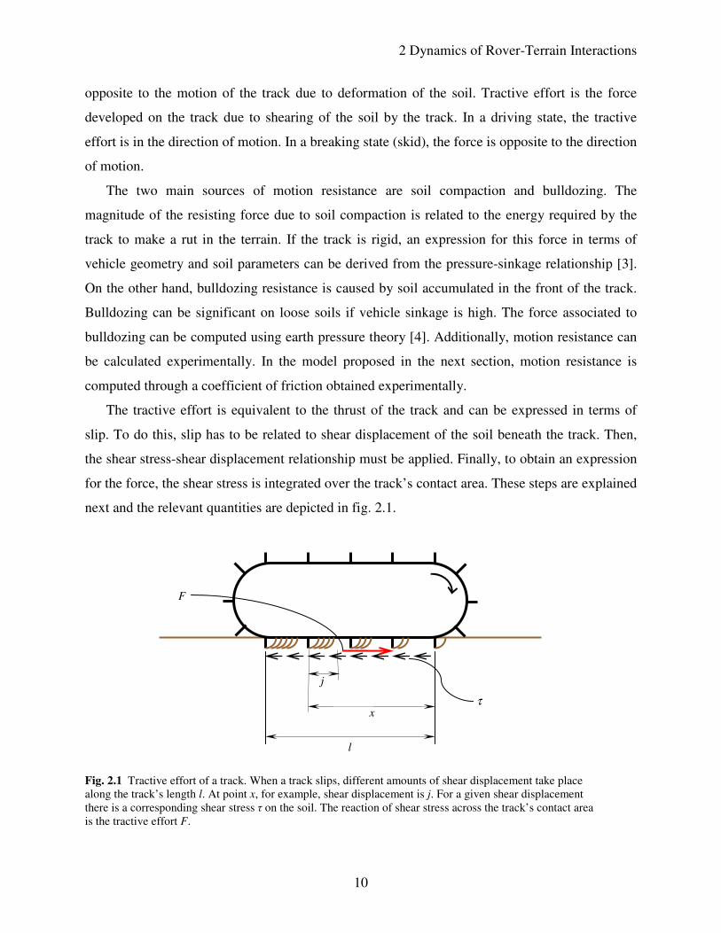
The tractive effort is equivalent to the thrust of the track and can be expressed in terms of
slip. To do this, slip has to be related to shear displacement of the soil beneath the track. Then,
the shear stress-shear displacement relationship must be applied. Finally, to obtain an expression
for the force, the shear stress is integrated over the track’s contact area. These steps are explained
next and the relevant quantities are depicted in fig. 2.1.
Fig. 2.1 Tractive effort of a track. When a track slips, different amounts of shear displacement take place
along the track’s length l. At point x, for example, shear displacement is j. For a given shear displacement
there is a corresponding shear stress τ on the soil. The reaction of shear stress across the track’s contact area
is the tractive effort F.
j
x
l
τ
F
2 Dynamics of Rover-Terrain Interactions
11
The relationship between slip and shear displacement is established first. The slip of a track i
is defined as:
t
j
t
t
t V
V
V
VV
V
V
r
Vi =
−=−=−= 11
ω (2.1)
where V is the track’s actual forward speed, Vt is the theoretical speed which is the product of the
angular speed ω and radius r of the pitch circle of the driving sprocket, and Vj is the speed of slip
of the track with respect to the ground. If it is assumed that the track does not stretch, Vj is
constant for each point along the track-terrain interface. This means that the more time a point of
the track spends in the ground, the more shear displacement j undergoes at that point.
Mathematically, this is:
tVj j= (2.2)
where t is the time a particular point has been in contact with the terrain. If x represents the
distance between such point and the front of the track, t can be calculated by:
tV
xt = (2.3)
Hence, by substituting eq. (2.3) into eq. (2.2) and using eq. (2.1), the relationship between slip
and shear displacement can be established:
ixV
xVj
t
j== (2.4)
Now, the shear stress-shear displacement relationship must be applied to relate shear stress
with slip. For loose sand such as lunar regolith, the shear stress-shear displacement relationship
can be approximated by [3]:
( )( )Kjepc −−+= 1tanφτ (2.5)
where τ is shear stress, p is the normal pressure exerted by the track on the soil, and c, ϕ, and K
are apparent cohesion, angle of internal shearing resistance, and shear deformation modulus of
the soil, respectively. Eq. (2.4) is substituted in eq. (2.5) to get the desired relationship:
( )( )Kixepc −−+= 1tanφτ (2.6)
2 Dynamics of Rover-Terrain Interactions
12
The last step is to integrate eq. (2.6) across the track’s contact area to obtain the expression of
the tractive effort:
( )( )∫∫−−+==
lKix
l
dxepcbdxbF00
1tanφτ (2.7)
where b is the width of the track and l is the length of the track’s contact area. If a uniform
normal pressure distribution is assumed, ( )blWp = where W is the normal load on the track,
and the integration of eq. (2.7) results in:
( ) ( )
−−+= − Kil
eil
KWAcF 11tanφ (2.8)
Eq. (2.8) is the expression of the tractive effort used in the model of the rover presented in
the next section.
2.2 Rover’s Model
This section describes the derivation of the model for the robot. It consists of a kinematic and a
dynamic model. Both models are derived starting from the analysis of a skid-steering maneuver.
The case of driving on a straight line corresponds to a turn of infinite radius R. A simplifying
assumption of the model is that the translation of the center of gravity (CG) of the robot due to
the plow’s displacement is negligible. This is reasonable since the plow represents a small
percentage of the total mass. It is also important to mention that the model does not account for
landslides. The reasons for this are their complex dynamics and random occurrence. Therefore,
landslides are considered disturbances to the system in this work.
As it will be seen, the model is parameterized in terms of lateral and longitudinal friction
coefficients, and the coefficients of the polynomial expression describing the force acting on the
plow. In section 2.3, these parameters are adjusted to fit experimental data.
The reference frame conventions throughout the thesis are as follows. The robot’s frame is
denoted by f: {x, y, z, t}. Its origin is fixed at the CG. The z axis points toward the top part of the
robot’s body. The inertial frame is denoted by F: {X, Y, Z, t}. The XY plane is parallel to the
terrain and the Z axis points outward the terrain.
2 Dynamics of Rover-Terrain Interactions
13
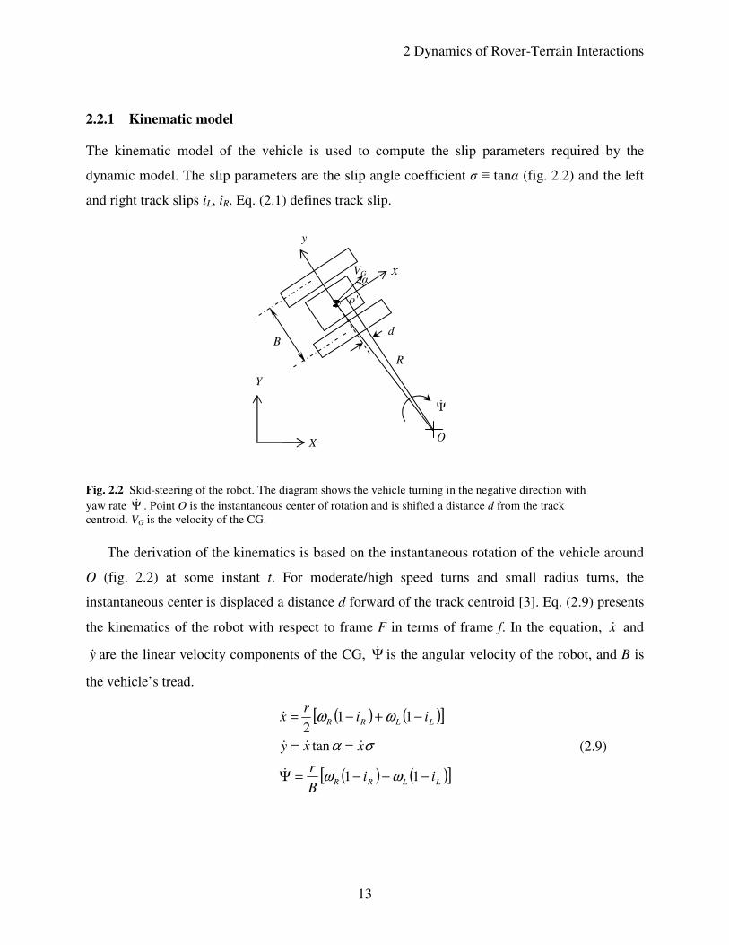
2.2.1 Kinematic model
The kinematic model of the vehicle is used to compute the slip parameters required by the
dynamic model. The slip parameters are the slip angle coefficient σ ≡ tanα (fig. 2.2) and the left
and right track slips iL, iR. Eq. (2.1) defines track slip.
Fig. 2.2 Skid-steering of the robot. The diagram shows the vehicle turning in the negative direction with
yaw rate Ψ& . Point O is the instantaneous center of rotation and is shifted a distance d from the track
centroid. VG is the velocity of the CG.
The derivation of the kinematics is based on the instantaneous rotation of the vehicle around
O (fig. 2.2) at some instant t. For moderate/high speed turns and small radius turns, the
instantaneous center is displaced a distance d forward of the track centroid [3]. Eq. (2.9) presents
the kinematics of the robot with respect to frame F in terms of frame f. In the equation, x& and
y& are the linear velocity components of the CG, Ψ& is the angular velocity of the robot, and B is
the vehicle’s tread.
( ) ( )[ ]
( ) ( )[ ]LLRR
LLRR
iiB
r
xxy
iir
x
−−−=Ψ
==
−+−=
11
tan
112
ωω
σα
ωω
&
&&&
&
(2.9)
X O
Y
B
x
y
Ψ&
o'
d
VG α
R
2 Dynamics of Rover-Terrain Interactions
14
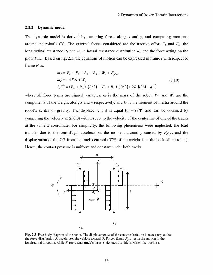
2.2.2 Dynamic model
The dynamic model is derived by summing forces along x and y, and computing moments
around the robot’s CG. The external forces considered are the tractive effort FL and FR, the
longitudinal resistance RL and RR, a lateral resistance distribution Rl, and the force acting on the
plow Fplow. Based on fig. 2.3, the equations of motion can be expressed in frame f with respect to
frame F as:
( ) ( ) ( ) ( ) ( )22 4222
4
dlRBRFBRFI
WdRym
FWRRFFxm
lLLRRG
yl
plowxRLRL
−+⋅+−⋅+=Ψ
+−=
+++++=
&&
&&
&&
(2.10)
where all force terms are signed variables, m is the mass of the robot, Wx and Wy are the
components of the weight along x and y respectively, and IG is the moment of inertia around the
robot’s center of gravity. The displacement d is equal to Ψ− &&y and can be obtained by
computing the velocity at (d,0,0) with respect to the velocity of the centerline of one of the tracks
at the same x coordinate. For simplicity, the following phenomena were neglected: the load
transfer due to the centrifugal acceleration, the moment around y caused by Fplow, and the
displacement of the CG from the track centroid (57% of the weight is at the back of the robot).
Hence, the contact pressure is uniform and constant under both tracks.
Fig. 2.3 Free body diagram of the robot. The displacement d of the center of rotation is necessary so that
the force distribution Rl accelerates the vehicle toward O. Forces Ri and Fplow resist the motion in the
longitudinal direction, while Fi represents track’s thrust (i denotes the side in which the track is).
RL RR
FL FR
Fplow
y
x
O
l d
B
Ψ&
Rl
2 Dynamics of Rover-Terrain Interactions
15
Computation of forces
In this section the expressions for each of the forces in eq. (2.10) will be presented. The tractive
effort of a track can be computed using the derivation of section 2.1. Since it is assumed that the
shearing behavior of the soil is the same for driving and breaking, eq. (2.8) can be rewritten as
follows:
( ) ( )isigneil
KWblcF
Kil
−
⋅−
+=
⋅−11tan
2φ (2.11)
where b is the width of the track and W is the component of the robot’s weight normal to the
terrain plane. The function sign(i) is 1 if i > 0, -1 if i < 0, and 0 if i = 0.
The resisting forces are expressed in terms of coefficients of friction. The coefficients are
assumed to be constant [4][3]. The longitudinal resistance R is computed as:
( )xsignW
fR r&
2−= (2.12)
where fr is a longitudinal friction coefficient. The lateral resistance distribution Rl due to sideslip
of the vehicle is calculated as:
( )Ψ−= &signl
WR tl
2µ (2.13)
where µt is a lateral friction coefficient.
The expression for the force acting on the plow is a second order polynomial of the variable
depth which is the plow depth measured from ground level (it ranges from 0 to 0.20 m for
Icebreaker). When depth < 0.05 m, Fplow = 0. This case is when only the conic part of the plow is
in the soil. Otherwise, the force is calculated by:
2
210 depthadepthaaFplow ⋅+⋅+= (2.14)
The rationale for the above mathematical form will be clear in the next section where a0, a1, and
a2 are computed through experimental data, along with fr and µt.
2.3 Parameter Identification
After programming the model in MATLAB’s Simulink, the identification was performed
through MATLAB’s Simulink Design Optimization toolbox which estimates model parameters
from data. The data comes from experiments of driving the robot on lunar relevant terrain. Two
sets of parameters were obtained for the planar and inclined terrain cases, respectively.
2 Dynamics of Rover-Terrain Interactions
16
Using the above toolbox, the experimental data was preprocessed before performing the
optimization. The preprocessing step consisted in outlier elimination and first order filtering. For
the optimization, the nonlinear least squares method and the trust-region-reflective algorithm
were selected to find the parameters fr, µt, a0, a1, and a2. Vehicle parameters measured directly on
the robot are presented in table 2.1. For IG, the robot was approximated as a prism encircling the
robot’s body without the plow.
Table 2.1 Vehicle parameters
m (kg) l (m) B (m) b (m) r (m) IG (kg·m2)
76 1.19 0.925 0.155 0.122 20.411
The optimization of a set of parameters requires one or more experimental data sets. Each
data set consisted of logged input and output signals of the robot. The optimization process feeds
the model with these inputs and adjusts the parameters so that the model’s outputs match the
experimental outputs. The experimental setup and the nature of these signals are described in
subsection 2.3.1.
Optimal parameters were obtained for driving on planar terrain (subsection 2.3.2) and
descending a steep slope (subsection 2.3.3), separately. The experiments on planar terrain
allowed computing fr and µt. The optimal value of µt was used as a fixed constant in the
optimization for inclined terrain where a new value of fr was calculated along with the plow
parameters a0, a1, and a2. A different longitudinal friction coefficient is obtained for the inclined
and planar cases because phenomena such as bulldozing is less significant in a steep slope where
the soil is already near its angle of repose.
The design of the experiments will be presented first and then the optimization results for the
planar and inclined terrain cases will be shown.
2.3.1 Experiment design
For achieving lunar relevant conditions, the experiments were carried out at the Simulated Lunar
Operations (SLOPE) facility at NASA Glenn Research Center, OH. High precision instruments
were used to log the data required by the optimization.
2 Dynamics of Rover-Terrain Interactions
17
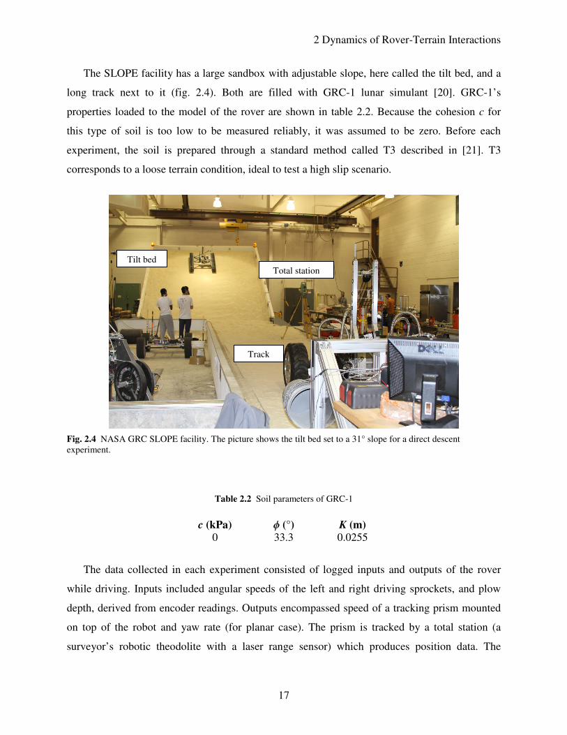
The SLOPE facility has a large sandbox with adjustable slope, here called the tilt bed, and a
long track next to it (fig. 2.4). Both are filled with GRC-1 lunar simulant [20]. GRC-1’s
properties loaded to the model of the rover are shown in table 2.2. Because the cohesion c for
this type of soil is too low to be measured reliably, it was assumed to be zero. Before each
experiment, the soil is prepared through a standard method called T3 described in [21]. T3
corresponds to a loose terrain condition, ideal to test a high slip scenario.
Fig. 2.4 NASA GRC SLOPE facility. The picture shows the tilt bed set to a 31° slope for a direct descent
experiment.
Table 2.2 Soil parameters of GRC-1
c (kPa) ϕ (°) K (m)
0 33.3 0.0255
The data collected in each experiment consisted of logged inputs and outputs of the rover
while driving. Inputs included angular speeds of the left and right driving sprockets, and plow
depth, derived from encoder readings. Outputs encompassed speed of a tracking prism mounted
on top of the robot and yaw rate (for planar case). The prism is tracked by a total station (a
surveyor’s robotic theodolite with a laser range sensor) which produces position data. The
Tilt bed
Track
Total station
2 Dynamics of Rover-Terrain Interactions
18
precision of the instrument is 5 mm and less than 0.0014°. Speed is obtained by using the
timestamps of the position data. Yaw rate is measured by a high precision fiber optic gyroscope
mounted in the robot. The gyroscope has a random walk of 4°/hr/√Hz.
The particular experiments for each of the terrain grade cases will be explained next along
with the optimization results.
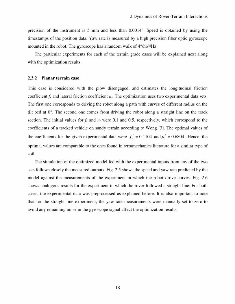
2.3.2 Planar terrain case
This case is considered with the plow disengaged, and estimates the longitudinal friction
coefficient fr and lateral friction coefficient µt. The optimization uses two experimental data sets.
The first one corresponds to driving the robot along a path with curves of different radius on the
tilt bed at 0°. The second one comes from driving the robot along a straight line on the track
section. The initial values for fr and ut were 0.1 and 0.5, respectively, which correspond to the
coefficients of a tracked vehicle on sandy terrain according to Wong [3]. The optimal values of
the coefficients for the given experimental data were 1104.0* =rf and 6804.0* =tµ . Hence, the
optimal values are comparable to the ones found in terramechanics literature for a similar type of
soil.
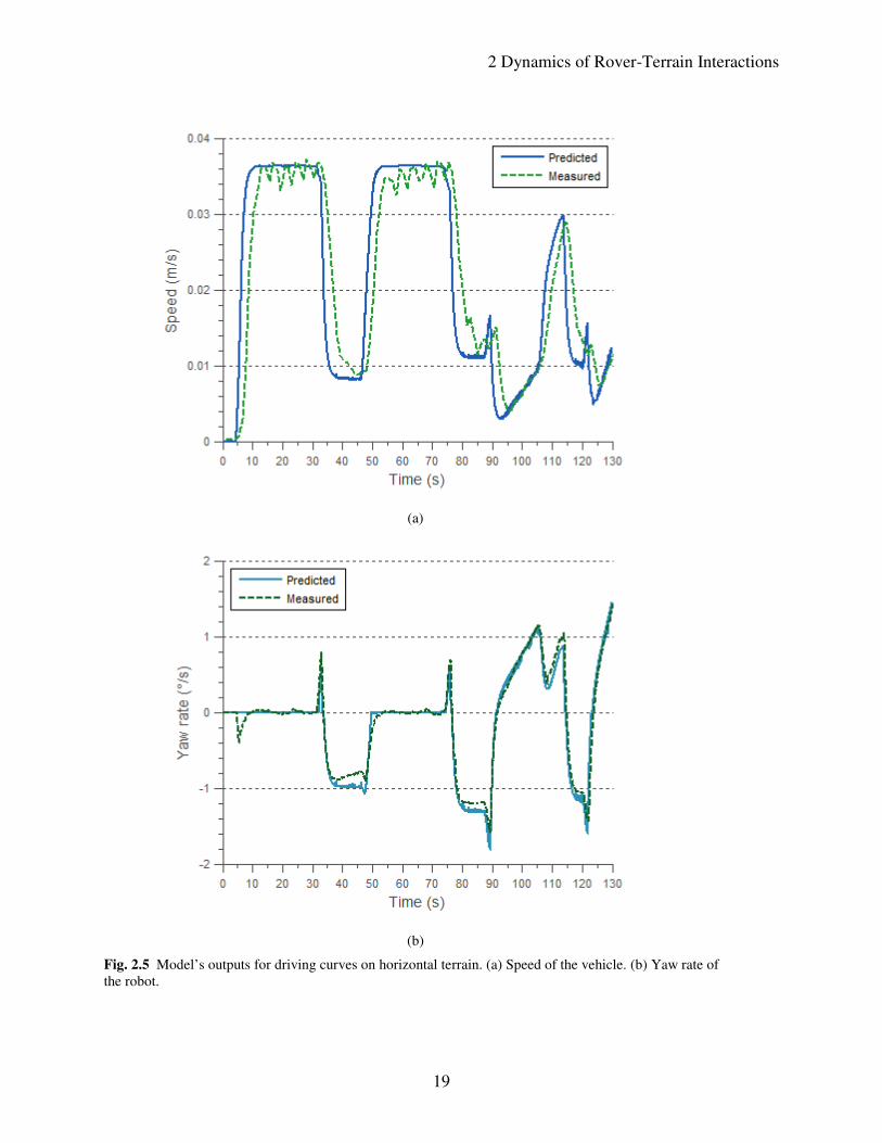
The simulation of the optimized model fed with the experimental inputs from any of the two
sets follows closely the measured outputs. Fig. 2.5 shows the speed and yaw rate predicted by the
model against the measurements of the experiment in which the robot drove curves. Fig. 2.6
shows analogous results for the experiment in which the rover followed a straight line. For both
cases, the experimental data was preprocessed as explained before. It is also important to note
that for the straight line experiment, the yaw rate measurements were manually set to zero to
avoid any remaining noise in the gyroscope signal affect the optimization results.
2 Dynamics of Rover-Terrain Interactions
19
(a)
(b)
Fig. 2.5 Model’s outputs for driving curves on horizontal terrain. (a) Speed of the vehicle. (b) Yaw rate of
the robot.
2 Dynamics of Rover-Terrain Interactions
20
Fig. 2.6 Model’s outputs for driving a straight line. (a) Speed of the vehicle. (b) Yaw rate of the robot.
2 Dynamics of Rover-Terrain Interactions
21
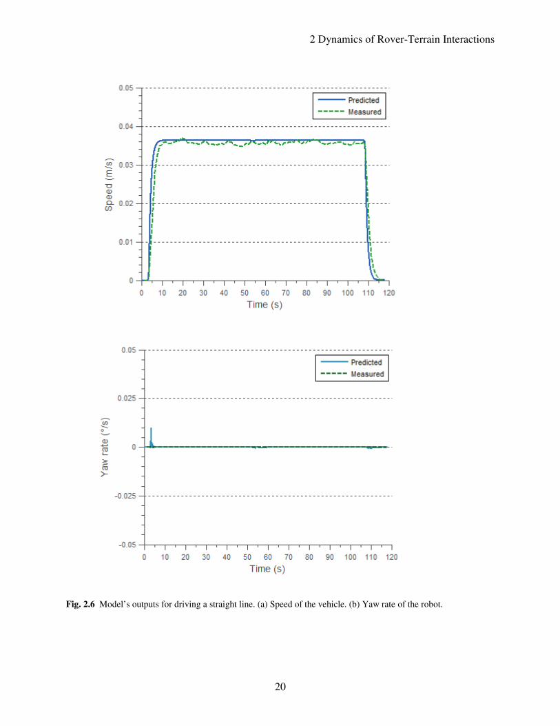
2.3.3 Inclined terrain case
For this case, fr is optimized first with one data set in which the plow is disengaged and then a0,
a1, and a2 are optimized with three data sets in which the plow is used. The output considered in
these optimizations is only speed. The portions of the data during which a landslide occurred
were eliminated. After all the parameters have been optimized, the model is validated with
additional data sets. All data sets correspond to direct descent experiments on the tilt bed at 31°.
The robot is commanded to drive down-slope at 0.3 rad/s until the lower part of the tilt bed is
reached. For each experiment the plow is set to a particular depth which is kept constant
throughout the run. It was observed that the speed is stable whenever a landslide is not
developing.
In the data set used to optimize fr the plow was not commanded into the ground. The initial
value for fr was the optimal value obtained in the planar terrain case. After optimization, its value
was 0.0939 which is lower than the planar case as expected. Fig. 2.7 shows how the speed
predicted by the model with the optimized coefficient is roughly the average of the
measurements when a landslide has not happened.
Fig. 2.7 Model’s output for descending without plow. The model predicts correctly the portions where a landslide is
not occurring (before 54 s).
2 Dynamics of Rover-Terrain Interactions
22
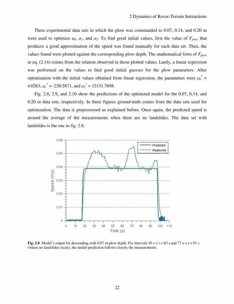
Three experimental data sets in which the plow was commanded to 0.07, 0.14, and 0.20 m
were used to optimize a0, a1, and a2. To find good initial values, first the value of Fplow that
produces a good approximation of the speed was found manually for each data set. Then, the
values found were plotted against the corresponding plow depth. The mathematical form of Fplow
in eq. (2.14) comes from the relation observed in those plotted values. Lastly, a linear regression
was performed on the values to find good initial guesses for the plow parameters. After
optimization with the initial values obtained from linear regression, the parameters were a0* =
4.0263, a1* = -230.5871, and a2
* = 12131.7698.
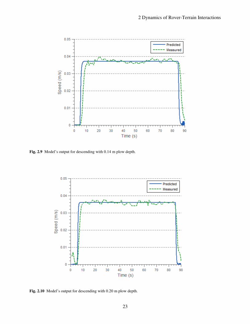
Fig. 2.8, 2.9, and 2.10 show the predictions of the optimized model for the 0.07, 0.14, and
0.20 m data sets, respectively. In these figures ground-truth comes from the data sets used for
optimization. The data is preprocessed as explained before. Once again, the predicted speed is
around the average of the measurements when there are no landslides. The data set with
landslides is the one in fig. 2.8.
Fig. 2.8 Model’s output for descending with 0.07 m plow depth. For intervals 45 s < t < 63 s and 77 s < t < 91 s
(where no landslides occur), the model prediction follows closely the measurements.
2 Dynamics of Rover-Terrain Interactions
23
Fig. 2.9 Model’s output for descending with 0.14 m plow depth.
Fig. 2.10 Model’s output for descending with 0.20 m plow depth.
2 Dynamics of Rover-Terrain Interactions
24
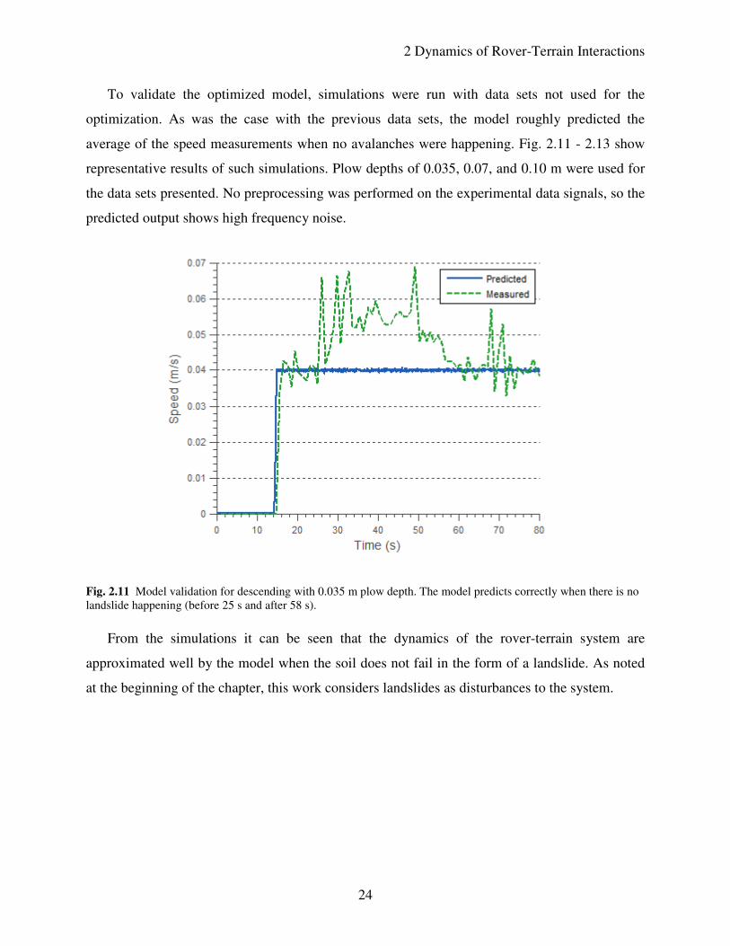
To validate the optimized model, simulations were run with data sets not used for the
optimization. As was the case with the previous data sets, the model roughly predicted the
average of the speed measurements when no avalanches were happening. Fig. 2.11 - 2.13 show
representative results of such simulations. Plow depths of 0.035, 0.07, and 0.10 m were used for
the data sets presented. No preprocessing was performed on the experimental data signals, so the
predicted output shows high frequency noise.
Fig. 2.11 Model validation for descending with 0.035 m plow depth. The model predicts correctly when there is no
landslide happening (before 25 s and after 58 s).
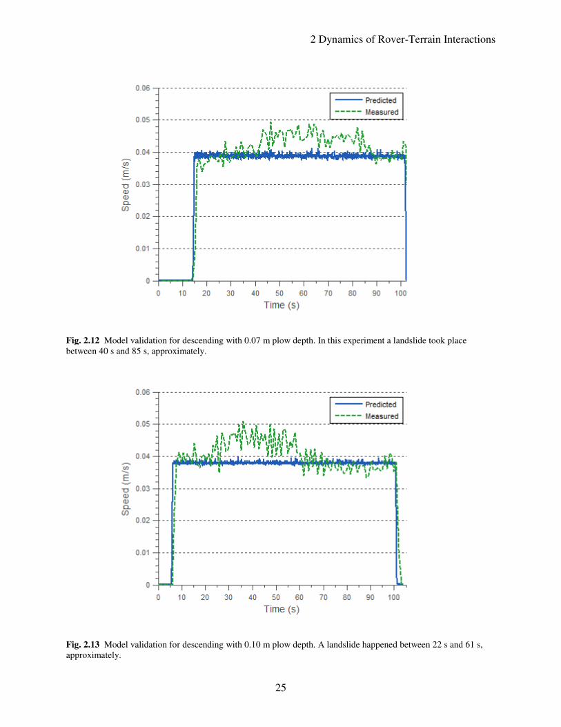
From the simulations it can be seen that the dynamics of the rover-terrain system are
approximated well by the model when the soil does not fail in the form of a landslide. As noted
at the beginning of the chapter, this work considers landslides as disturbances to the system.
2 Dynamics of Rover-Terrain Interactions
25
Fig. 2.12 Model validation for descending with 0.07 m plow depth. In this experiment a landslide took place
between 40 s and 85 s, approximately.
Fig. 2.13 Model validation for descending with 0.10 m plow depth. A landslide happened between 22 s and 61 s,
approximately.
26
Chapter 3
Vision System
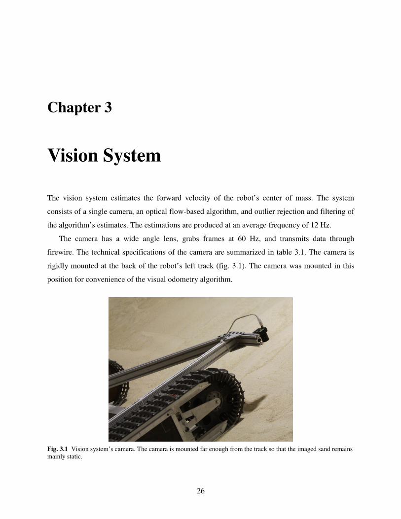
The vision system estimates the forward velocity of the robot’s center of mass. The system
consists of a single camera, an optical flow-based algorithm, and outlier rejection and filtering of
the algorithm’s estimates. The estimations are produced at an average frequency of 12 Hz.
The camera has a wide angle lens, grabs frames at 60 Hz, and transmits data through
firewire. The technical specifications of the camera are summarized in table 3.1. The camera is
rigidly mounted at the back of the robot’s left track (fig. 3.1). The camera was mounted in this
position for convenience of the visual odometry algorithm.
Fig. 3.1 Vision system’s camera. The camera is mounted far enough from the track so that the imaged sand remains
mainly static.
3 Vision System
27
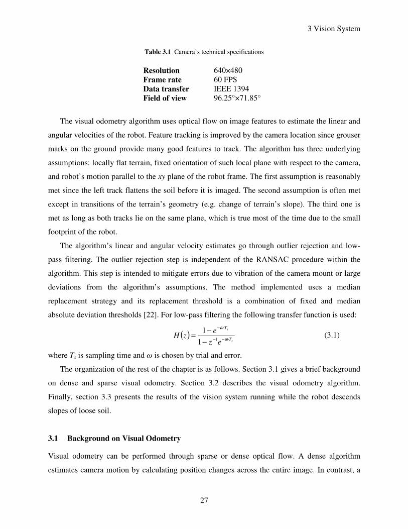
Table 3.1 Camera’s technical specifications
Resolution 640×480
Frame rate 60 FPS
Data transfer IEEE 1394
Field of view 96.25°×71.85°
The visual odometry algorithm uses optical flow on image features to estimate the linear and
angular velocities of the robot. Feature tracking is improved by the camera location since grouser
marks on the ground provide many good features to track. The algorithm has three underlying
assumptions: locally flat terrain, fixed orientation of such local plane with respect to the camera,
and robot’s motion parallel to the xy plane of the robot frame. The first assumption is reasonably
met since the left track flattens the soil before it is imaged. The second assumption is often met
except in transitions of the terrain’s geometry (e.g. change of terrain’s slope). The third one is
met as long as both tracks lie on the same plane, which is true most of the time due to the small
footprint of the robot.
The algorithm’s linear and angular velocity estimates go through outlier rejection and low-
pass filtering. The outlier rejection step is independent of the RANSAC procedure within the
algorithm. This step is intended to mitigate errors due to vibration of the camera mount or large
deviations from the algorithm’s assumptions. The method implemented uses a median
replacement strategy and its replacement threshold is a combination of fixed and median
absolute deviation thresholds [22]. For low-pass filtering the following transfer function is used:
( )s
s
T
T
ez
ezH
⋅−−
⋅−
−
−=
ω
ω
11
1 (3.1)
where Ts is sampling time and ω is chosen by trial and error.
The organization of the rest of the chapter is as follows. Section 3.1 gives a brief background
on dense and sparse visual odometry. Section 3.2 describes the visual odometry algorithm.
Finally, section 3.3 presents the results of the vision system running while the robot descends
slopes of loose soil.
3.1 Background on Visual Odometry
Visual odometry can be performed through sparse or dense optical flow. A dense algorithm
estimates camera motion by calculating position changes across the entire image. In contrast, a
3 Vision System
28
sparse approach calculates position changes of a set of features. Both methods can be
implemented using monocular or stereo imaging.
A dense optical flow algorithm estimates image motion by assuming that the intensity of a
scene point is constant (brightness conservation) and that the motion is smooth everywhere in the
image [23]. Dense optical flow is, in general, computationally demanding. One example of a
monocular implementation comes from the work of Campbell et al. [24]. They assumed a planar
world to estimate the motion of a mobile robot’s camera. On the other hand, Morency and Gupta
[25] used stereo imaging for computing large displacements of a camera.
Sparse optical flow algorithms track a group of features between consecutive images. This
makes the approach more computationally efficient than its dense counterpart. The assumption
of brightness conservation is also applied in sparse algorithms. Song et al. [26] used a monocular
sparse approach to estimate the motion of a mobile robot by assuming locally flat terrain.
Conversely, the MSL rover uses a stereo implementation of sparse optical flow to estimate its 6-
DOF motion [10].
Hence, visual odometry can be based on sparse or dense optical flow. Instances of monocular
and stereo implementations exist for each approach.
3.2 Algorithm Description
The visual odometry algorithm uses one camera looking at the ground and is based on sparse
optical flow [11]. Its main attributes are computational efficiency and robustness. The latter
comes from two actions. One is to apply a dynamic mask on the image to select features away
from the edges of the robot’s own shadow. The other is to enforce a rigidity constraint for outlier
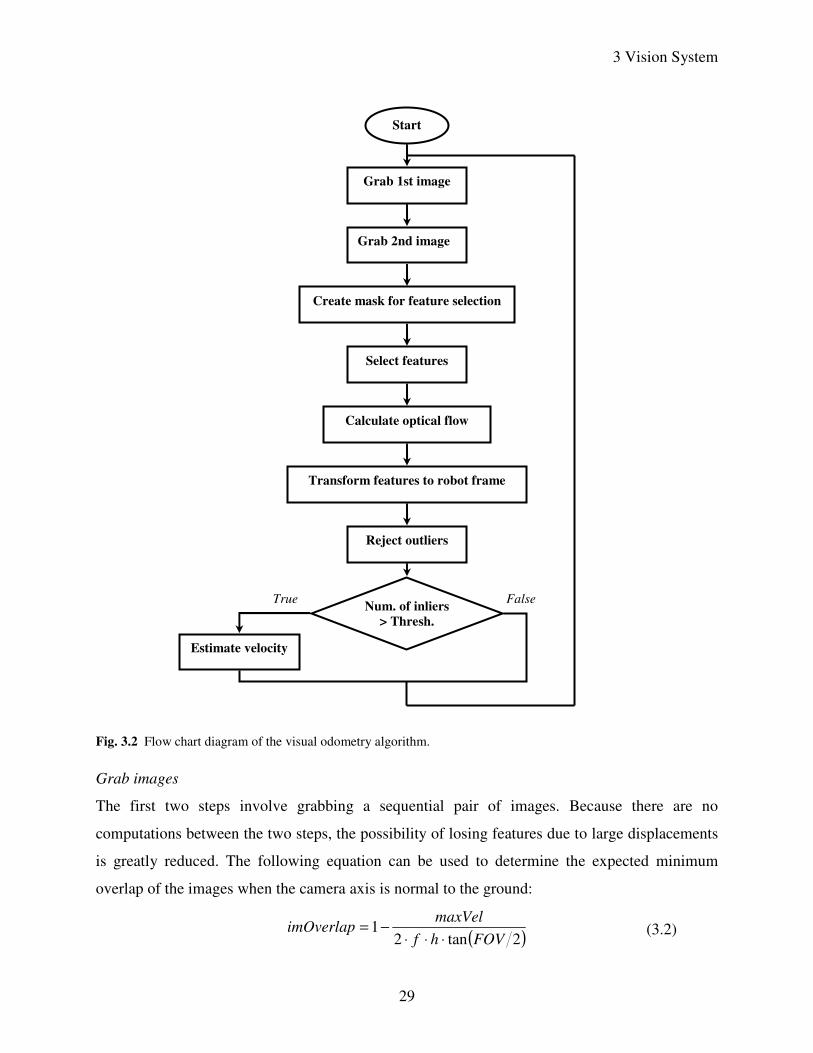
rejection of tracked features. The algorithm was implemented using the OpenCV library. Fig. 3.2
shows a flow chart diagram of the program. Each of the steps will be explained next.
3 Vision System
29
Fig. 3.2 Flow chart diagram of the visual odometry algorithm.
Grab images
The first two steps involve grabbing a sequential pair of images. Because there are no
computations between the two steps, the possibility of losing features due to large displacements
is greatly reduced. The following equation can be used to determine the expected minimum
overlap of the images when the camera axis is normal to the ground:
( )2tan21
FOVhf
VelmaximOverlap
⋅⋅⋅−= (3.2)
Start
Grab 1st image
Grab 2nd image
Create mask for feature selection
Select features
Calculate optical flow
Transform features to robot frame
Reject outliers
Num. of inliers
> Thresh.
Estimate velocity
True False
3 Vision System
30
where maxVel is the robot’s maximum velocity, f is the framerate, h is the height of the camera
with respect to the ground, and FOV is the camera’s angular field of view. The quantities
imOverlap, maxVel, and FOV are along the direction of travel. It is important to note that if the
camera axis is not perpendicular to the ground, the result of (3.2) is a lower bound of the actual
overlap. The lower bound for Icebreaker is 99%.
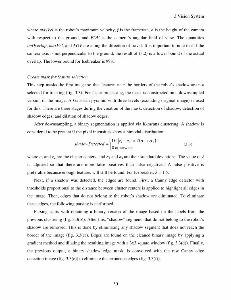
Create mask for feature selection
This step masks the first image so that features near the borders of the robot’s shadow are not
selected for tracking (fig. 3.3). For faster processing, the mask is constructed on a downsampled
version of the image. A Gaussian pyramid with three levels (excluding original image) is used
for this. There are three stages during the creation of the mask: detection of shadow, detection of
shadow edges, and dilation of shadow edges.
After downsampling, a binary segmentation is applied via K-means clustering. A shadow is
considered to be present if the pixel intensities show a bimodal distribution:
( )
+>−
=otherwise 0
if 1 2121 σσλccctedshadowDete (3.3)
where c1 and c2 are the cluster centers, and σ1 and σ2 are their standard deviations. The value of λ
is adjusted so that there are more false positives than false negatives. A false positive is
preferable because enough features will still be found. For Icebreaker, λ = 1.5.
Next, if a shadow was detected, the edges are found. First, a Canny edge detector with
thresholds proportional to the distance between cluster centers is applied to highlight all edges in
the image. Then, edges that do not belong to the robot’s shadow are eliminated. To eliminate
these edges, the following parsing is performed.
Parsing starts with obtaining a binary version of the image based on the labels from the
previous clustering (fig. 3.3(b)). After this, “shadow” segments that do not belong to the robot’s
shadow are removed. This is done by eliminating any shadow segment that does not reach the
border of the image (fig. 3.3(c)). Edges are found on the cleaned binary image by applying a
gradient method and dilating the resulting image with a 3x3 square window (fig. 3.3(d)). Finally,
the previous output, a binary shadow edge mask, is convolved with the raw Canny edge
detection image (fig. 3.3(e)) to eliminate the erroneous edges (fig. 3.3(f)).
3 Vision System
31
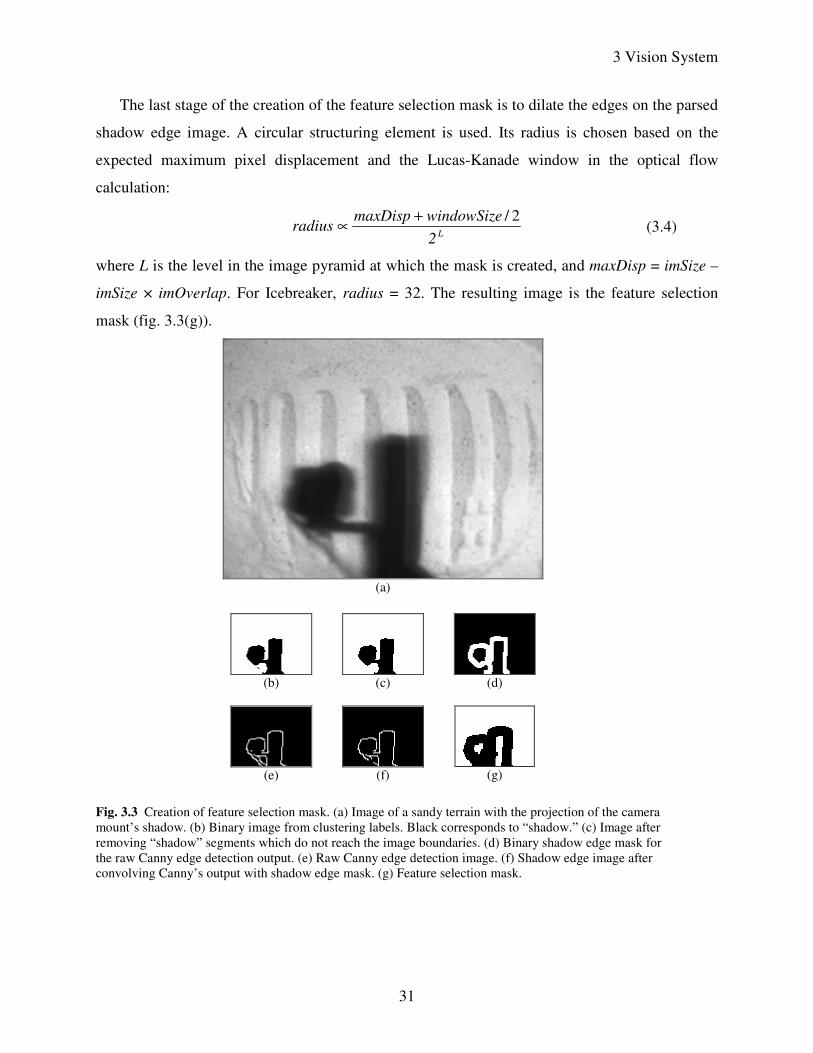
The last stage of the creation of the feature selection mask is to dilate the edges on the parsed
shadow edge image. A circular structuring element is used. Its radius is chosen based on the
expected maximum pixel displacement and the Lucas-Kanade window in the optical flow
calculation:
L
2
windowSizeDispmaxradius
2/+∝ (3.4)
where L is the level in the image pyramid at which the mask is created, and maxDisp = imSize –
imSize × imOverlap. For Icebreaker, radius = 32. The resulting image is the feature selection
mask (fig. 3.3(g)).
(a)
(b)
(c)
(d)
(e)
(f)
(g)
Fig. 3.3 Creation of feature selection mask. (a) Image of a sandy terrain with the projection of the camera
mount’s shadow. (b) Binary image from clustering labels. Black corresponds to “shadow.” (c) Image after
removing “shadow” segments which do not reach the image boundaries. (d) Binary shadow edge mask for
the raw Canny edge detection output. (e) Raw Canny edge detection image. (f) Shadow edge image after
convolving Canny’s output with shadow edge mask. (g) Feature selection mask.
3 Vision System
32
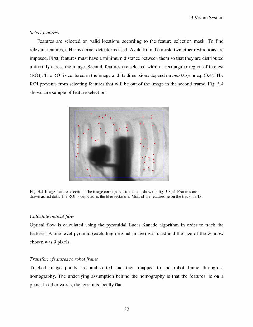
Select features
Features are selected on valid locations according to the feature selection mask. To find
relevant features, a Harris corner detector is used. Aside from the mask, two other restrictions are
imposed. First, features must have a minimum distance between them so that they are distributed
uniformly across the image. Second, features are selected within a rectangular region of interest
(ROI). The ROI is centered in the image and its dimensions depend on maxDisp in eq. (3.4). The
ROI prevents from selecting features that will be out of the image in the second frame. Fig. 3.4
shows an example of feature selection.
Fig. 3.4 Image feature selection. The image corresponds to the one shown in fig. 3.3(a). Features are
drawn as red dots. The ROI is depicted as the blue rectangle. Most of the features lie on the track marks.
Calculate optical flow
Optical flow is calculated using the pyramidal Lucas-Kanade algorithm in order to track the
features. A one level pyramid (excluding original image) was used and the size of the window
chosen was 9 pixels.
Transform features to robot frame
Tracked image points are undistorted and then mapped to the robot frame through a
homography. The underlying assumption behind the homography is that the features lie on a
plane, in other words, the terrain is locally flat.
3 Vision System
33
To undistort image points, the camera matrix and distortion coefficients are required. These
parameters are obtained through camera calibration.
The homography maps an undistorted image point to the {X, Y} coordinates of the
corresponding 3D point in the robot frame. The derivation is as follows. First, the pinhole camera
model relates the two coordinate systems through:
[ ]PtRKp ≡ (3.5)
where p is a 3×1 homogeneous coordinate vector of a point in the image, P is a 4×1
homogeneous coordinate vector of the corresponding 3D point in the robot frame, K is the 3×3
camera matrix, R is a 3×3 rotation matrix that transforms points expressed in the robot frame to
the camera frame, and t is a 3×1 position vector of the robot frame’s origin expressed in the
camera frame. The symbol “≡” denotes equivalence.
Now, if it is assumed that all 3D points lie in a plane, the Z coordinate of P can be expressed
in terms of X and Y:
[ ]
**
33333323331
23223222321
13113121311
3333231
2232221
1131211
1
1
PMY
X
crtbrrarr
crtbrrarr
crtbrrarr
cbYaXZ
Y
X
trrr
trrr
trrr
PtR
=
+++
+++
+++
=
++=
=
(3.6)
Substituting eq. (3.6) into (3.5) results in:
**PKMp ≡ (3.7)
Replacing the equivalence by equality in eq. (3.7):
**PsKMp = (3.8)
where s is a scale factor. Solving for P* in eq. (3.8) gives:
( ) HppKMsP ==−1** (3.9)
where H is the homography.
The {X, Y} coordinates of the point in 3D expressed in the robot frame are obtained by
dividing the components of sP* by the third component.
The homography is estimated through homogeneous linear least squares and is preloaded in
the visual odometry program. The set up of the minimization problem starts by rewriting eq.
3 Vision System
34
(3.9) with the components of sP* expressed explicitly and p being the augmented vector of the
image point (in pixels):
=
1
~
~
333231
232221
131211
y
x
hhh
hhh
hhh
s
Y
X
(3.10)
To obtain a set of equations which can be solved for the elements of H, the inhomogeneous
coordinates of the 3D point are first expressed as:
333231
131211
hyhxh
hyhxhX
++
++= ,
333231
232221
hyhxh
hyhxhY
++
++= (3.11)
By multiplying each equality in (3.11) by its denominator and rearranging terms, a system of
homogeneous equations is obtained:
0ha
0ha
=
=T
Y
T
X (3.12)
where
[ ]Thhhhhhhhh 333231232221131211=h
[ ]T
X XyXxXyx ⋅⋅−−−= 0001a
[ ]T
Y YyYxYyx ⋅⋅−−−= 1000a
Since a homography has 8 degrees of freedom and each point correspondence gives two
equations, a minimum of four correspondences are necessary to solve for h. However, the more
point correspondences are used, the more robust to errors the solution of h will be. With N
correspondences, the following linear system of equations can be formed:
0h =A (3.13)
where
=
T
Y
T
X
T
Y
T
X
N
N
A
a
a
a
a
M
1
1
Eq. (3.13) represents a homogeneous linear least squares problem. It can be solved with
singular value decomposition (SVD). If the SVD of A is computed as in eq. (3.14), the column of
3 Vision System
35
V that corresponds to the smallest singular value is the solution of h that minimizes eq. (3.13) in
the least squares sense.
TVΣUA = (3.14)
In practice, the point correspondences to compute H were obtained by taking an image of a
chessboard target lying flat on the ground. The target was placed in such a manner that the inner
corner locations were known with respect to the robot frame. Then the pixel coordinates of the
corresponding points in the image were extracted and undistorted.
Reject outliers
This step uses RANSAC to obtain the largest set of features that observe a rigidity constraint
between the pair of consecutive images. Hence, the model to which RANSAC fits the data is a
rigid body transformation. The method from Challis [27] is used to compute the transformation
parameters. The type of error sources addressed by this outlier rejection include shadows, out of
plane features, and moving objects, if the features they affect do not form the largest consistent
set. Each iteration of RANSAC consists in the following steps.
First, a random set of three pairs of tracked features (transformed to robot frame) are selected
from N pairs.
The model to be instantiated by the sampled set is derived as follows. First, the rigidity
constraint is established. It is assumed that the terrain is parallel to the xy plane of the robot
frame. Let qi be a 2×1 vector of the ith point from the first image after the transformation of the
visual odometry algorithm’s previous step. Similarly, let ci be the corresponding point in the
second image. The rigidity constraint can be expressed as:
vRqc ii += (3.15)
where R is a 2×2 rotation matrix describing the rotation of the robot frame at the instant the first
image was taken, with respect to its orientation when the second image was grabbed, and v is a
2×1 position vector of the robot frame’s origin at the first instant, with respect to the robot frame
when the second image was taken. R and v are the model parameters sought. It will be seen that
only R is required.
The model parameters can be found through a least squares minimization of:
( ) ( )∑=
−+−+n
i
iiTiicvRqcvRq
n 1
1 (3.16)
3 Vision System
36
where n is the number of points (n ≥ 3, in general).
Now, v will be eliminated from eq. (3.16) so that R is the only parameter needed. To do this,
eq. (3.15) is summed across the n points and the resulting equation is solved for v:
qRcv −= (3.17)
where c is the centroid of the points ci and q , of the points q
i. Equation (3.17) is replaced in eq.
(3.16) and after algebraic manipulation the equation below is obtained:
( )∑=
′′−′′+′′n
i
i
T
ii
T
ii
T
i qRcqqccn 1
21
(3.18)
where
qqq ii −=′
ccc ii −=′ (3.19)
Now, the minimization problem represented by eq. (3.16) can be expressed as the
maximization of the third summation term in eq. (3.18):
( )∑=
′′n
i
i
T
i qRcn 1
1 (3.20)
Before continuing, let’s define the matrices below:
[ ]nqqQ ′′=′ L1 (3.21)
[ ]Nall qqQ ′′=′ L1 (3.22)
Matrices C ′ and allC ′ are defined in an analogous way.
Going back to eq. (3.20), it can be re-expressed as:
( ) { }Κ=
′′=′′∑=
TTTn
i
i
T
i RQCn
RqRcn
trace1
trace1
1
(3.23)
where nQCK T′′= is called the correlation matrix. Next, the SVD of K is computed:
TT
VΣUQCn
K =′′=1
(3.24)
If the SVD of K is substituted in eq. (3.23) and the equality trace{ABT} = trace{B
TA} is
applied, we have:
{ } { }ΣURVR TTT tracetrace =Κ (3.25)
The attention is now focused on the matrix URVTT=Γ . It can be seen that this matrix is
orthogonal, so the absolute value of each element in the diagonal is less than 1. Also, since Σ is
3 Vision System
37
diagonal, only the diagonal of Γ has an effect in eq. (3.25). This means that eq. (3.25) has a
maximum when Γ is the identity matrix, in other words, when:
TUVR = (3.26)
Equations (3.19), (3.21), (3.24) and (3.26) can then be used to compute the rigid body
transformation parameter R.
In the RANSAC iteration, once the random sample of three pairs of correspondences has
been selected, the four equations just mentioned are used to instantiate the model (eq. (3.26)).
The next step of RANSAC is to determine the set of point pairs from the complete set that
have an error with respect to the model below a certain threshold. The error is computed by:
=′−′=
N
errerr
N
errerr
allallYY
XXQRCError
L
L
1
1
(3.27)
A point i is considered an inlier if ( ) ( )22 i
err
i
err YX + is less than the threshold. For Icebreaker,
the threshold used was 0.002 m due to the slow motion of the vehicle.
RANSAC terminates when the number of iterations reach a predefined number maxIter or
when the number of inliers found in the current iteration is greater than a threshold threshInliers,
whichever happens first. If the procedure terminates because of the number of iterations, then the
inliers selected correspond to the largest set in all the previous iterations.
Estimate velocity
Once points are expressed in the robot frame and their outliers are rejected, the linear and
angular velocities of the robot are estimated. This motion is measured with respect to an inertial
frame, but expressed in the robot frame. The linear velocity corresponds to the velocity of the
center of mass of the robot.
To relate the relative velocities of the points tracked with the motion of the vehicle, the
following equation of the motion of a particle for non-inertial frames is used:
roavrvv +×+= ω (3.28)
where va is the absolute velocity of the particle with respect to the inertial frame, v
o is the
velocity of the non-inertial frame’s origin with respect to the inertial frame, ω is the angular
velocity of the noninertial frame, r is the position vector of the particle with respect to the non-
inertial frame, and vr is the relative velocity of the particle with respect to the non-inertial frame.

3 Vision System
38
In this application, vo (velocity of the robot’s center of mass v
robot) and ω (angular velocity)
are the vectors to be estimated. Here, the inertial frame is a frame with the same position and
orientation as the robot frame when the second image is grabbed. The noninertial frame is the
robot frame itself. A feature is considered a particle in eq. (3.28). Since features are supposed to
be static points on the ground, va = 0. The position vector r corresponds to the feature location
with respect to the robot frame when the second image was grabbed. It is computed with eq.
(3.11). Finally, vr
is the velocity of the feature as perceived from the moving robot frame (non-
inertial frame). This is computed by subtracting the results of eq. (3.11) in the first image from
the results of the same equation in the second image, and dividing by the time difference
between frames.
Hence, eq. (3.28) can be rewritten as:
rvvrobotr ×+=− ω (3.29)
With the aforementioned assumption of motion parallel to the xy plane of the robot frame, eq.
(3.29) can be expressed as:
×
+
=
−
z
y
x
z
robot
y
robot
x
r
y
r
x
r
r
r
v
v
v
v
ω
0
0
00
(3.30)
Eq. (3.30) is for a single feature. Based on this, a system of linear equations can be set up:
−=
−
−
−
−
mr
y
mr
x
r
y
r
x
z
robot
y
robot
x
m
x
m
y
x
y
v
v
v
v
v
v
r
r
r
r
MMMM
1
1
1
1
10
01
10
01
ω
(3.31)
where m is the total number of inliers.
Eq. (3.31) requires a minimum of two features to be solved. To solve it, pseudoinverse is
applied.
3.3 Performance on Lunar Regolith
To assess the performance of the vision system, a set of 11 experiments were carried out at
NASA Glenn Research Center’s SLOPE facility. Each experiment consisted on a direct descent
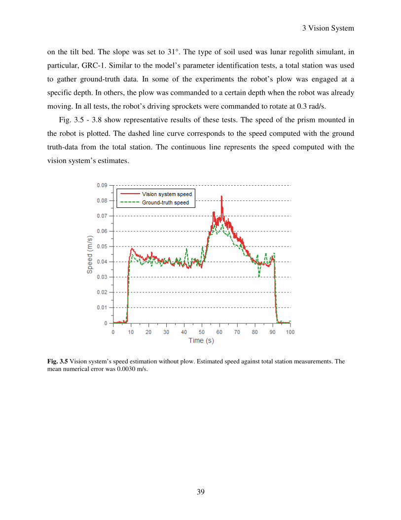
3 Vision System
39
on the tilt bed. The slope was set to 31°. The type of soil used was lunar regolith simulant, in
particular, GRC-1. Similar to the model’s parameter identification tests, a total station was used
to gather ground-truth data. In some of the experiments the robot’s plow was engaged at a
specific depth. In others, the plow was commanded to a certain depth when the robot was already
moving. In all tests, the robot’s driving sprockets were commanded to rotate at 0.3 rad/s.
Fig. 3.5 - 3.8 show representative results of these tests. The speed of the prism mounted in
the robot is plotted. The dashed line curve corresponds to the speed computed with the ground
truth-data from the total station. The continuous line represents the speed computed with the
vision system’s estimates.
Fig. 3.5 Vision system’s speed estimation without plow. Estimated speed against total station measurements. The
mean numerical error was 0.0030 m/s.
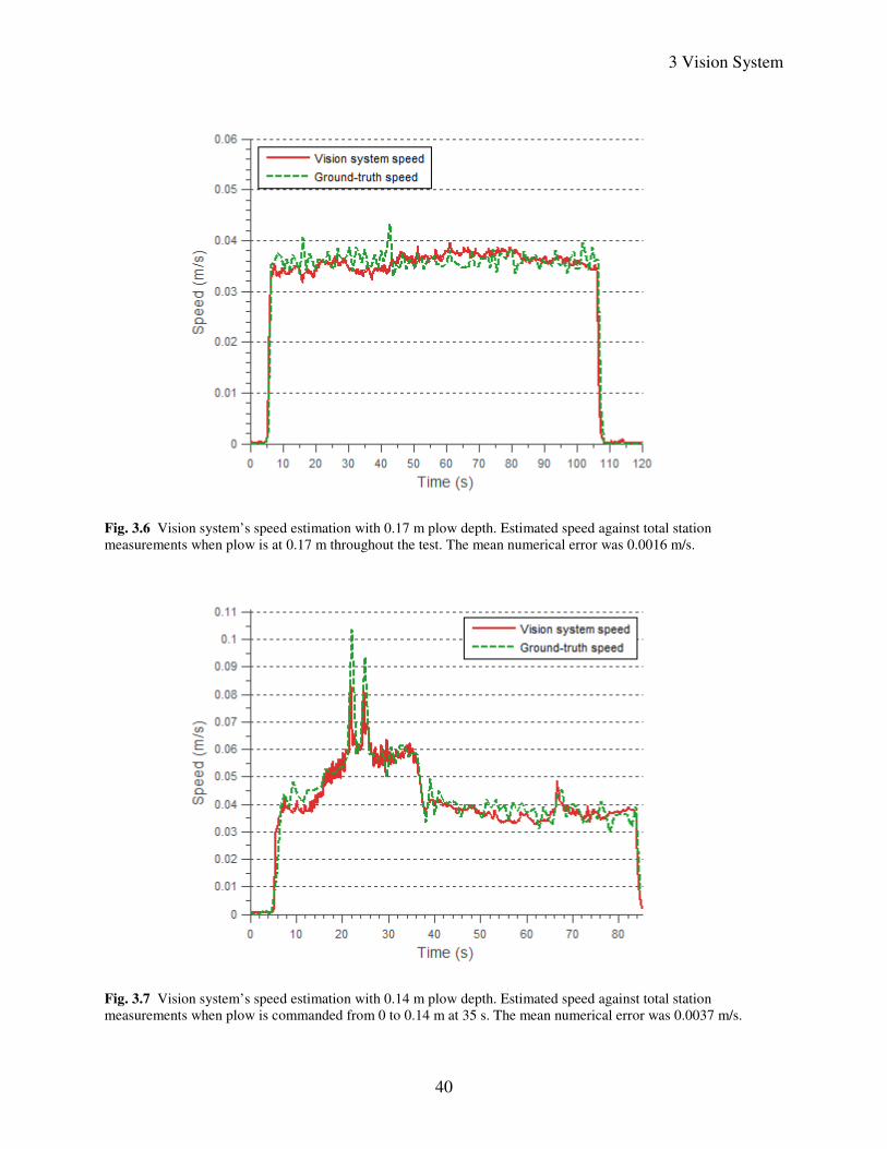
3 Vision System
40
Fig. 3.6 Vision system’s speed estimation with 0.17 m plow depth. Estimated speed against total station
measurements when plow is at 0.17 m throughout the test. The mean numerical error was 0.0016 m/s.
Fig. 3.7 Vision system’s speed estimation with 0.14 m plow depth. Estimated speed against total station
measurements when plow is commanded from 0 to 0.14 m at 35 s. The mean numerical error was 0.0037 m/s.
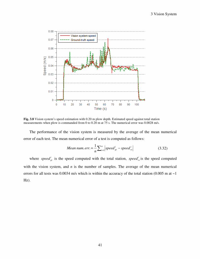
3 Vision System
41
Fig. 3.8 Vision system’s speed estimation with 0.20 m plow depth. Estimated speed against total station
measurements when plow is commanded from 0 to 0.20 m at 75 s. The numerical error was 0.0028 m/s.
The performance of the vision system is measured by the average of the mean numerical
error of each test. The mean numerical error of a test is computed as follows:
∑ =−=
n
i
i
vs
i
gt speedspeedn
err. num. Mean1
1 (3.32)
where i
gtspeed is the speed computed with the total station, i
vsspeed is the speed computed
with the vision system, and n is the number of samples. The average of the mean numerical
errors for all tests was 0.0034 m/s which is within the accuracy of the total station (0.005 m at ~1
Hz).
42
Chapter 4
Classical Controllers
This chapter presents the design of two standard types of controllers, applied here to regulate
vehicle slip. The first type is an on-off controller which takes one of three possible predefined
actions depending on the value of slip. The second type is a PID controller (PI after tuning).
Since the on-off controller was implemented in the robot only as a slip-control proof of concept,
simulations are presented for the PI case exclusively. Results of the actual implementation of the
on-off controller will be given in chapter 6.
For both standard controllers and the fuzzy logic controller discussed in the next chapter, the
process to be controlled is formulated as a single-input single-output (SISO) system, as explained
in section 1.3. The input to the system is commanded plow depth and the output is slip as defined
in eq. (1.1). The input to the controller is error in slip which is defined by:
vehicleref iie −= (4.1)
where iref is the slip reference or setpoint selected by the user. The output of the controller is
commanded plow depth. The output signal is in digital form and a zero-order hold is used to
interface it with the process, which has continuous signals.
The next section will outline the design specifications set out for the classical and fuzzy logic
controllers.
4 Classical Controllers
43
4.1 Performance Objectives
The design specifications presented here have the purpose of assessing the performance of the
slip controllers explored in this thesis. They serve to evaluate them in both simulation and actual
implementation. The slip controller should abide to the following:
• Steady-state error should be within ±5% slip from iref. Given the noisy nature of slip, this ±5%
range, called here the allowable band, is considered good tracking of the reference signal.
• The time required for the slip to enter the allowable band should be less than 10 seconds. This
time is measured from the instant in which the driving sprockets have reached the commanded
angular speed.
• Slip above 5% should be avoided. This has the intention to decrease the energy consumption
due to dragging the plow in the soil during descents.
• The above objectives should be achieved for different commanded angular speeds and slope
grades.
The design of each controller is targeted to comply with the above specifications. The on-off
controller will be explained first followed by the PI controller.
4.2 On-Off Controller
This is the simplest of the three controllers. It is comprised by a small set of if-then rules. Its
implementation in the robot helped to gain intuition on how to better control the system. This
knowledge was particularly useful during the design of the fuzzy logic controller.
4.2.1 Design
The controller is based on an incremental approach, that is, an increment to plow depth is first
obtained from the if-then rules. The increment is added to the current plow depth and saturated if
the value is beyond the plow depth range (0 – 0.20 m). The resulting plow depth is commanded
to the process. The pseudocode to compute the increment in plow depth ∆depth is the following:
if ivehicle < ( iref – 0.05 )
∆depth = 0.01
else if ivehicle > ( iref + 0.05 )
∆depth = -0.006 else
∆depth = -0.002
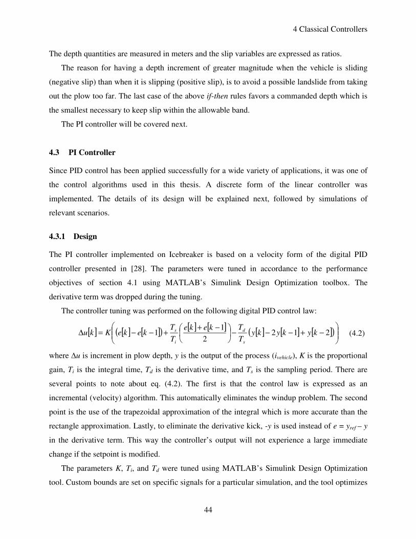
4 Classical Controllers
44
The depth quantities are measured in meters and the slip variables are expressed as ratios.
The reason for having a depth increment of greater magnitude when the vehicle is sliding
(negative slip) than when it is slipping (positive slip), is to avoid a possible landslide from taking
out the plow too far. The last case of the above if-then rules favors a commanded depth which is
the smallest necessary to keep slip within the allowable band.
The PI controller will be covered next.
4.3 PI Controller
Since PID control has been applied successfully for a wide variety of applications, it was one of
the control algorithms used in this thesis. A discrete form of the linear controller was
implemented. The details of its design will be explained next, followed by simulations of
relevant scenarios.
4.3.1 Design
The PI controller implemented on Icebreaker is based on a velocity form of the digital PID
controller presented in [28]. The parameters were tuned in accordance to the performance
objectives of section 4.1 using MATLAB’s Simulink Design Optimization toolbox. The
derivative term was dropped during the tuning.
The controller tuning was performed on the following digital PID control law:
[ ] [ ] [ ]( ) [ ] [ ] [ ] [ ] [ ]( )
−+−−−
−++−−=∆ 212
2
11 kykyky
T
Tkeke
T
TkekeKku
s
d
i
s (4.2)
where ∆u is increment in plow depth, y is the output of the process (ivehicle), K is the proportional
gain, Ti is the integral time, Td is the derivative time, and Ts is the sampling period. There are
several points to note about eq. (4.2). The first is that the control law is expressed as an
incremental (velocity) algorithm. This automatically eliminates the windup problem. The second
point is the use of the trapezoidal approximation of the integral which is more accurate than the
rectangle approximation. Lastly, to eliminate the derivative kick, -y is used instead of e = yref – y
in the derivative term. This way the controller’s output will not experience a large immediate
change if the setpoint is modified.
The parameters K, Ti, and Td were tuned using MATLAB’s Simulink Design Optimization
tool. Custom bounds are set on specific signals for a particular simulation, and the tool optimizes
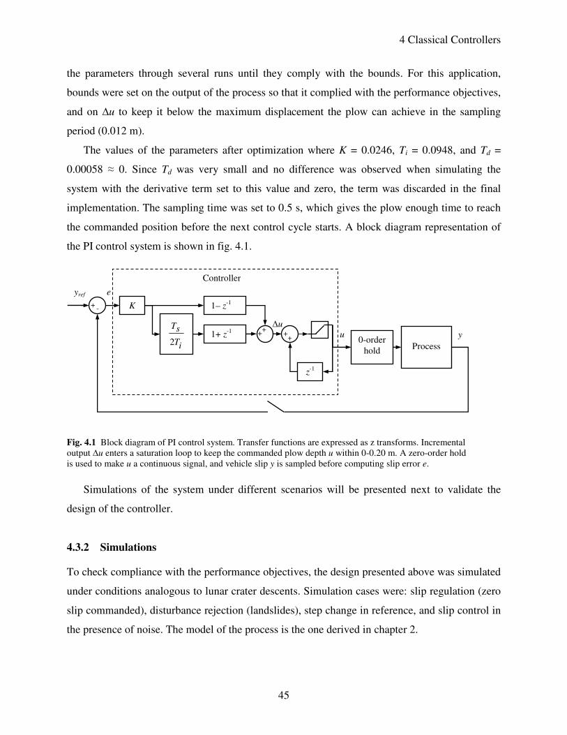
4 Classical Controllers
45
the parameters through several runs until they comply with the bounds. For this application,
bounds were set on the output of the process so that it complied with the performance objectives,
and on ∆u to keep it below the maximum displacement the plow can achieve in the sampling
period (0.012 m).
The values of the parameters after optimization where K = 0.0246, Ti = 0.0948, and Td =
0.00058 ≈ 0. Since Td was very small and no difference was observed when simulating the
system with the derivative term set to this value and zero, the term was discarded in the final
implementation. The sampling time was set to 0.5 s, which gives the plow enough time to reach
the commanded position before the next control cycle starts. A block diagram representation of
the PI control system is shown in fig. 4.1.
Fig. 4.1 Block diagram of PI control system. Transfer functions are expressed as z transforms. Incremental
output ∆u enters a saturation loop to keep the commanded plow depth u within 0-0.20 m. A zero-order hold
is used to make u a continuous signal, and vehicle slip y is sampled before computing slip error e.
Simulations of the system under different scenarios will be presented next to validate the
design of the controller.
4.3.2 Simulations
To check compliance with the performance objectives, the design presented above was simulated
under conditions analogous to lunar crater descents. Simulation cases were: slip regulation (zero
slip commanded), disturbance rejection (landslides), step change in reference, and slip control in
the presence of noise. The model of the process is the one derived in chapter 2.
1– z-1
K
iT
sT
2
+ -
+
+
+ + 1+ z
-1
0-order
hold
Process
z-1
Controller
y
yref e
u
∆u
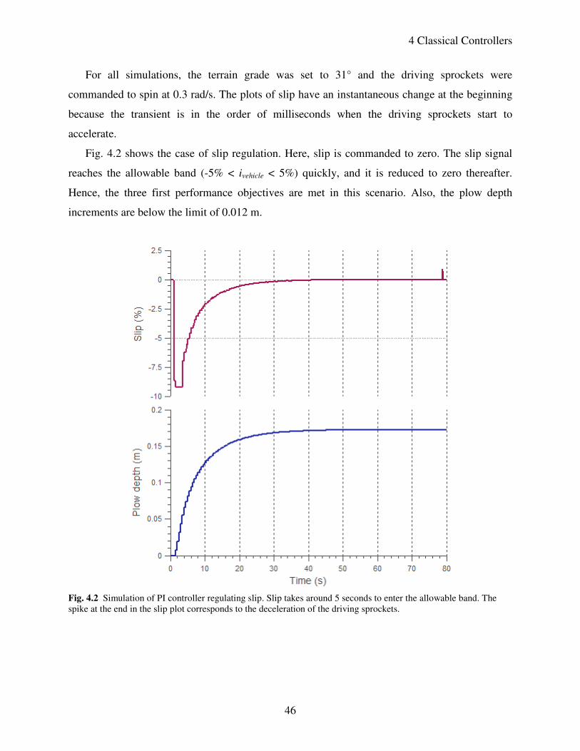
4 Classical Controllers
46
For all simulations, the terrain grade was set to 31° and the driving sprockets were
commanded to spin at 0.3 rad/s. The plots of slip have an instantaneous change at the beginning
because the transient is in the order of milliseconds when the driving sprockets start to
accelerate.
Fig. 4.2 shows the case of slip regulation. Here, slip is commanded to zero. The slip signal
reaches the allowable band (-5% < ivehicle < 5%) quickly, and it is reduced to zero thereafter.
Hence, the three first performance objectives are met in this scenario. Also, the plow depth
increments are below the limit of 0.012 m.
Fig. 4.2 Simulation of PI controller regulating slip. Slip takes around 5 seconds to enter the allowable band. The
spike at the end in the slip plot corresponds to the deceleration of the driving sprockets.
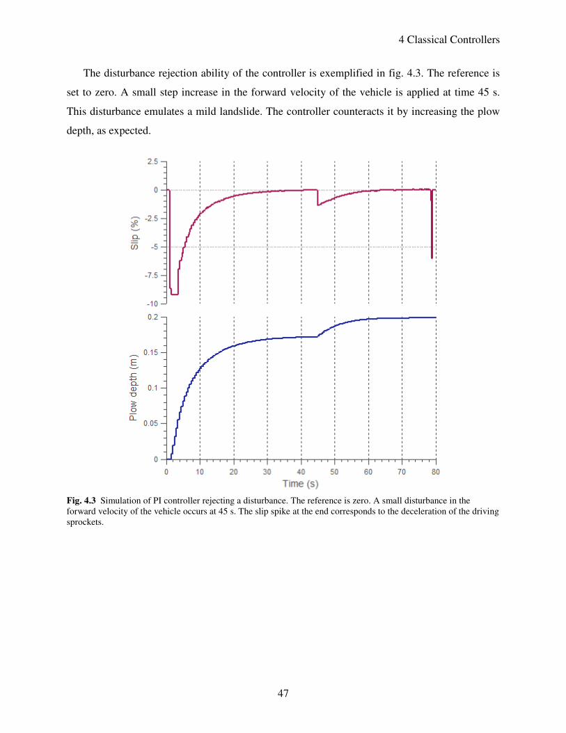
4 Classical Controllers
47
The disturbance rejection ability of the controller is exemplified in fig. 4.3. The reference is
set to zero. A small step increase in the forward velocity of the vehicle is applied at time 45 s.
This disturbance emulates a mild landslide. The controller counteracts it by increasing the plow
depth, as expected.
Fig. 4.3 Simulation of PI controller rejecting a disturbance. The reference is zero. A small disturbance in the
forward velocity of the vehicle occurs at 45 s. The slip spike at the end corresponds to the deceleration of the driving
sprockets.
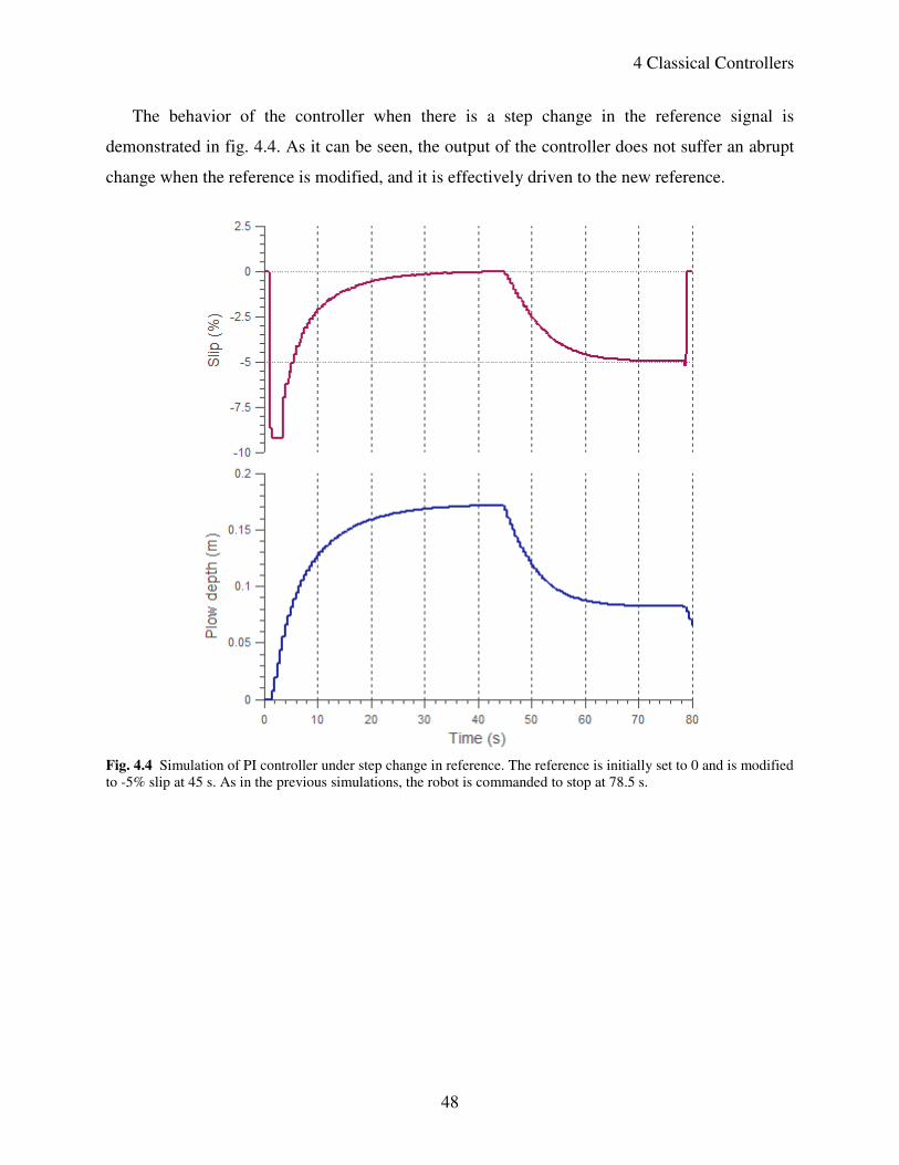
4 Classical Controllers
48
The behavior of the controller when there is a step change in the reference signal is
demonstrated in fig. 4.4. As it can be seen, the output of the controller does not suffer an abrupt
change when the reference is modified, and it is effectively driven to the new reference.
Fig. 4.4 Simulation of PI controller under step change in reference. The reference is initially set to 0 and is modified
to -5% slip at 45 s. As in the previous simulations, the robot is commanded to stop at 78.5 s.
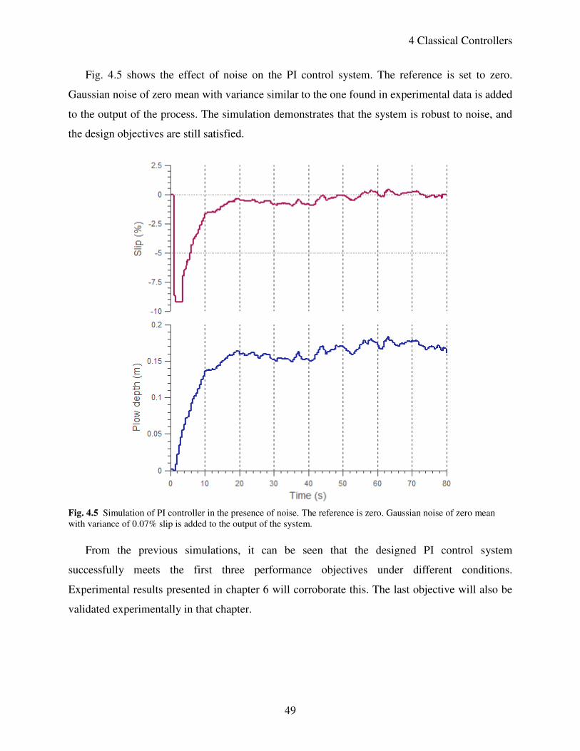
4 Classical Controllers
49
Fig. 4.5 shows the effect of noise on the PI control system. The reference is set to zero.
Gaussian noise of zero mean with variance similar to the one found in experimental data is added
to the output of the process. The simulation demonstrates that the system is robust to noise, and
the design objectives are still satisfied.
Fig. 4.5 Simulation of PI controller in the presence of noise. The reference is zero. Gaussian noise of zero mean
with variance of 0.07% slip is added to the output of the system.
From the previous simulations, it can be seen that the designed PI control system
successfully meets the first three performance objectives under different conditions.
Experimental results presented in chapter 6 will corroborate this. The last objective will also be
validated experimentally in that chapter.
50
Chapter 5
Fuzzy Logic Controller
This chapter covers the design and simulation of the vehicle slip control system based on a fuzzy
logic controller. The application of a fuzzy controller to vehicle slip control stems from two
reasons. First, fuzzy control allows a design based on informal knowledge of the system. This
permits accounting for phenomena such as landslides that cannot be properly described by a
mathematical model. Second, a fuzzy controller is a nonlinear controller which is a good match
for the nonlinear system studied in this thesis. Before going into the design details, the
fundamentals on fuzzy logic and fuzzy logic control will be presented. Only the concepts and
techniques relevant to this thesis are outlined.
5.1 Background on Fuzzy Logic
Fuzzy logic can be defined as the collection of theories and technologies that use fuzzy sets [29].
Fuzzy sets are a generalization of classical sets that allow smooth boundaries, as it will be
explained in the next subsection. Fuzzy logic has been successfully applied in numerous domains
because of the two main benefits it offers. First, it provides cost-effective approximate solutions
to complex problems by taking advantage of the tolerance for imprecision. Second, it is able to
handle concepts and knowledge with vague boundaries as human reasoning does.
Subsection 5.1.1 presents the basic concepts and methods of fuzzy logic. Subsection 5.1.2
frames these ideas in the context of control systems.
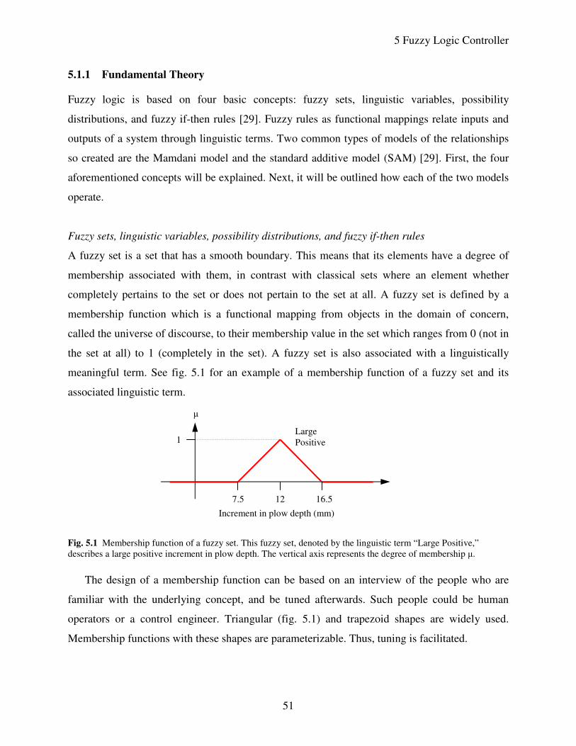
5 Fuzzy Logic Controller
51
5.1.1 Fundamental Theory
Fuzzy logic is based on four basic concepts: fuzzy sets, linguistic variables, possibility
distributions, and fuzzy if-then rules [29]. Fuzzy rules as functional mappings relate inputs and
outputs of a system through linguistic terms. Two common types of models of the relationships
so created are the Mamdani model and the standard additive model (SAM) [29]. First, the four
aforementioned concepts will be explained. Next, it will be outlined how each of the two models
operate.
Fuzzy sets, linguistic variables, possibility distributions, and fuzzy if-then rules
A fuzzy set is a set that has a smooth boundary. This means that its elements have a degree of
membership associated with them, in contrast with classical sets where an element whether
completely pertains to the set or does not pertain to the set at all. A fuzzy set is defined by a
membership function which is a functional mapping from objects in the domain of concern,
called the universe of discourse, to their membership value in the set which ranges from 0 (not in
the set at all) to 1 (completely in the set). A fuzzy set is also associated with a linguistically
meaningful term. See fig. 5.1 for an example of a membership function of a fuzzy set and its
associated linguistic term.
Fig. 5.1 Membership function of a fuzzy set. This fuzzy set, denoted by the linguistic term “Large Positive,”
describes a large positive increment in plow depth. The vertical axis represents the degree of membership µ.
The design of a membership function can be based on an interview of the people who are
familiar with the underlying concept, and be tuned afterwards. Such people could be human
operators or a control engineer. Triangular (fig. 5.1) and trapezoid shapes are widely used.
Membership functions with these shapes are parameterizable. Thus, tuning is facilitated.
1
7.5 12 16.5
Increment in plow depth (mm)
µ
Large
Positive
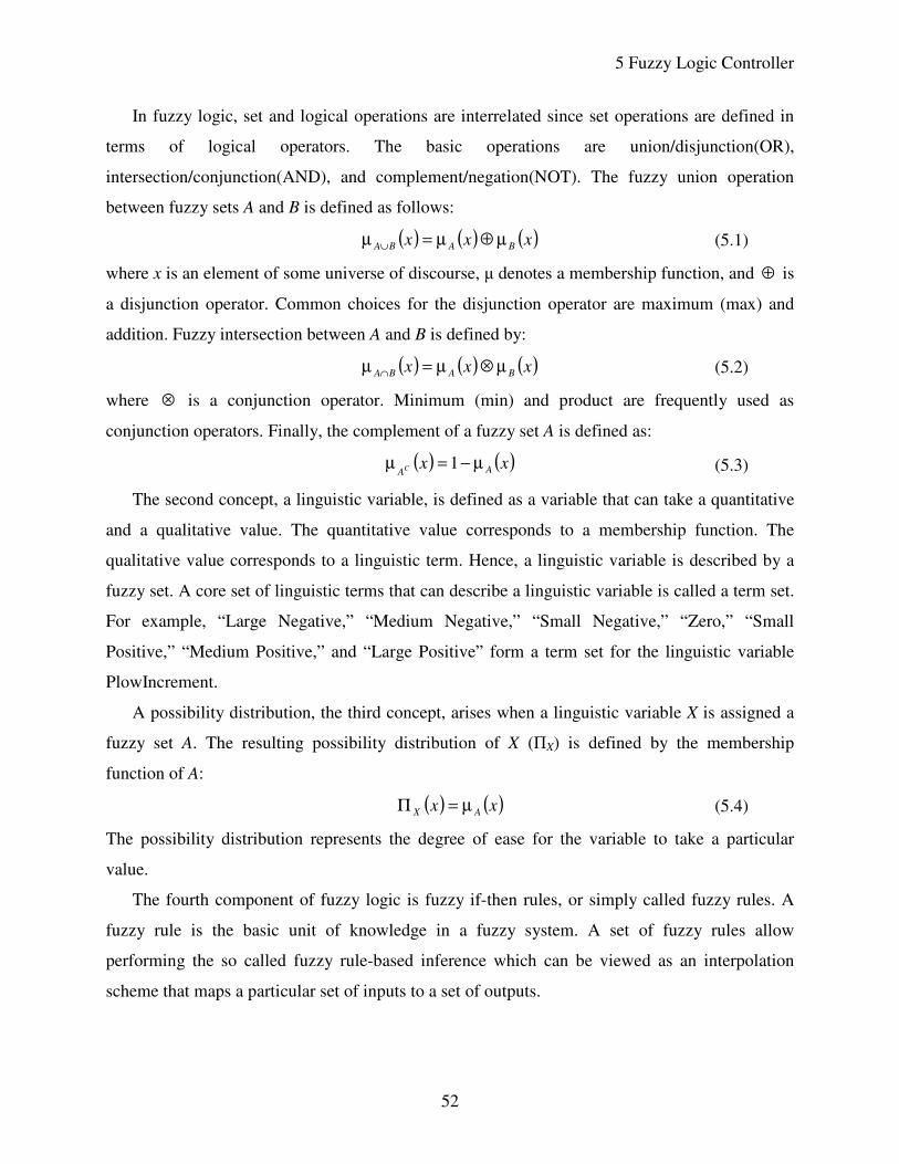
5 Fuzzy Logic Controller
52
In fuzzy logic, set and logical operations are interrelated since set operations are defined in
terms of logical operators. The basic operations are union/disjunction(OR),
intersection/conjunction(AND), and complement/negation(NOT). The fuzzy union operation
between fuzzy sets A and B is defined as follows:
( ) ( ) ( )xxx BABA µ⊕µ=µ ∪ (5.1)
where x is an element of some universe of discourse, µ denotes a membership function, and ⊕ is
a disjunction operator. Common choices for the disjunction operator are maximum (max) and
addition. Fuzzy intersection between A and B is defined by:
( ) ( ) ( )xxx BABA µ⊗µ=µ ∩ (5.2)
where ⊗ is a conjunction operator. Minimum (min) and product are frequently used as
conjunction operators. Finally, the complement of a fuzzy set A is defined as:
( ) ( )xx AAC µ−=µ 1 (5.3)
The second concept, a linguistic variable, is defined as a variable that can take a quantitative
and a qualitative value. The quantitative value corresponds to a membership function. The
qualitative value corresponds to a linguistic term. Hence, a linguistic variable is described by a
fuzzy set. A core set of linguistic terms that can describe a linguistic variable is called a term set.
For example, “Large Negative,” “Medium Negative,” “Small Negative,” “Zero,” “Small
Positive,” “Medium Positive,” and “Large Positive” form a term set for the linguistic variable
PlowIncrement.
A possibility distribution, the third concept, arises when a linguistic variable X is assigned a
fuzzy set A. The resulting possibility distribution of X (ПX) is defined by the membership
function of A:
( ) ( )xx AX µ=Π (5.4)
The possibility distribution represents the degree of ease for the variable to take a particular
value.
The fourth component of fuzzy logic is fuzzy if-then rules, or simply called fuzzy rules. A
fuzzy rule is the basic unit of knowledge in a fuzzy system. A set of fuzzy rules allow
performing the so called fuzzy rule-based inference which can be viewed as an interpolation
scheme that maps a particular set of inputs to a set of outputs.
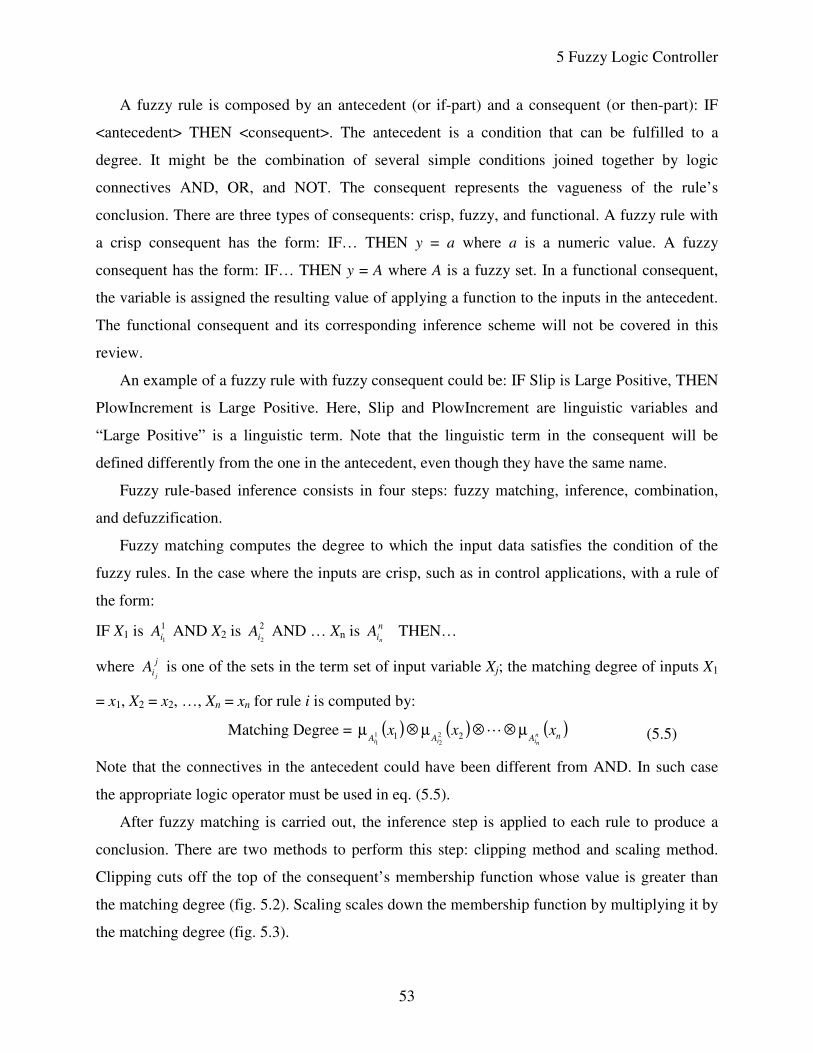
5 Fuzzy Logic Controller
53
A fuzzy rule is composed by an antecedent (or if-part) and a consequent (or then-part): IF
<antecedent> THEN <consequent>. The antecedent is a condition that can be fulfilled to a
degree. It might be the combination of several simple conditions joined together by logic
connectives AND, OR, and NOT. The consequent represents the vagueness of the rule’s
conclusion. There are three types of consequents: crisp, fuzzy, and functional. A fuzzy rule with
a crisp consequent has the form: IF… THEN y = a where a is a numeric value. A fuzzy
consequent has the form: IF… THEN y = A where A is a fuzzy set. In a functional consequent,
the variable is assigned the resulting value of applying a function to the inputs in the antecedent.
The functional consequent and its corresponding inference scheme will not be covered in this
review.
An example of a fuzzy rule with fuzzy consequent could be: IF Slip is Large Positive, THEN
PlowIncrement is Large Positive. Here, Slip and PlowIncrement are linguistic variables and
“Large Positive” is a linguistic term. Note that the linguistic term in the consequent will be
defined differently from the one in the antecedent, even though they have the same name.
Fuzzy rule-based inference consists in four steps: fuzzy matching, inference, combination,
and defuzzification.
Fuzzy matching computes the degree to which the input data satisfies the condition of the
fuzzy rules. In the case where the inputs are crisp, such as in control applications, with a rule of
the form:
IF X1 is 1
1iA AND X2 is 2
2iA AND … Xn is n
inA THEN…
where j
i jA is one of the sets in the term set of input variable Xj; the matching degree of inputs X1
= x1, X2 = x2, …, Xn = xn for rule i is computed by:
Matching Degree = ( ) ( ) ( )nAAA
xxx n
niii
µ⊗⊗µ⊗µ L21 2
2
1
1
(5.5)
Note that the connectives in the antecedent could have been different from AND. In such case
the appropriate logic operator must be used in eq. (5.5).
After fuzzy matching is carried out, the inference step is applied to each rule to produce a
conclusion. There are two methods to perform this step: clipping method and scaling method.
Clipping cuts off the top of the consequent’s membership function whose value is greater than
the matching degree (fig. 5.2). Scaling scales down the membership function by multiplying it by
the matching degree (fig. 5.3).
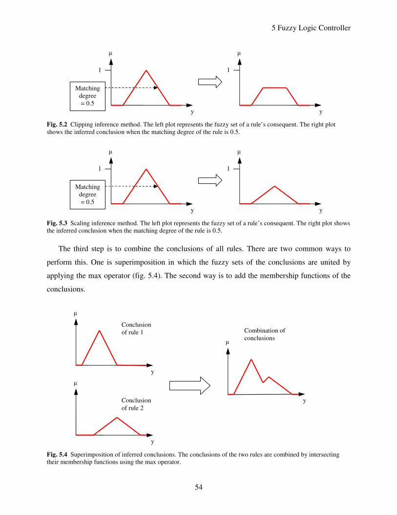
5 Fuzzy Logic Controller
54
Fig. 5.2 Clipping inference method. The left plot represents the fuzzy set of a rule’s consequent. The right plot
shows the inferred conclusion when the matching degree of the rule is 0.5.
Fig. 5.3 Scaling inference method. The left plot represents the fuzzy set of a rule’s consequent. The right plot shows
the inferred conclusion when the matching degree of the rule is 0.5.
The third step is to combine the conclusions of all rules. There are two common ways to
perform this. One is superimposition in which the fuzzy sets of the conclusions are united by
applying the max operator (fig. 5.4). The second way is to add the membership functions of the
conclusions.
Fig. 5.4 Superimposition of inferred conclusions. The conclusions of the two rules are combined by intersecting
their membership functions using the max operator.
1
µ
1
µ
Matching
degree
= 0.5
y y
1
µ
1
µ
Matching
degree
= 0.5
y y
µ
y
µ
y
Conclusion
of rule 1 Combination of
conclusions
µ
y
Conclusion
of rule 2
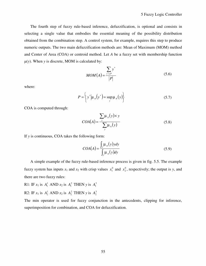
5 Fuzzy Logic Controller
55
The fourth step of fuzzy rule-based inference, defuzzification, is optional and consists in
selecting a single value that embodies the essential meaning of the possibility distribution
obtained from the combination step. A control system, for example, requires this step to produce
numeric outputs. The two main defuzzification methods are: Mean of Maximum (MOM) method
and Center of Area (COA) or centroid method. Let A be a fuzzy set with membership function
µ(y). When y is discrete, MOM is calculated by:
( )P
y
AMOMPy
∑∈
=*
*
(5.6)
where:
( ) ( )
µ=µ= yyyP Ay
A sup** (5.7)
COA is computed through:
( )( )
( )∑
∑
µ
×µ
=
y
A
y
A
y
yy
ACOA (5.8)
If y is continuous, COA takes the following form:
( )( )
( )∫
∫µ
µ=
yA
yA
dyy
ydyyACOA (5.9)
A simple example of the fuzzy rule-based inference process is given in fig. 5.5. The example
fuzzy system has inputs x1 and x2 with crisp values 0
1x and 0
2x , respectively; the output is y, and
there are two fuzzy rules:
R1: IF x1 is 1
1A AND x2 is 2
1A THEN y is 3
1A
R2: IF x1 is 1
2A AND x2 is 2
2A THEN y is 3
2A
The min operator is used for fuzzy conjunction in the antecedents, clipping for inference,
superimposition for combination, and COA for defuzzification.
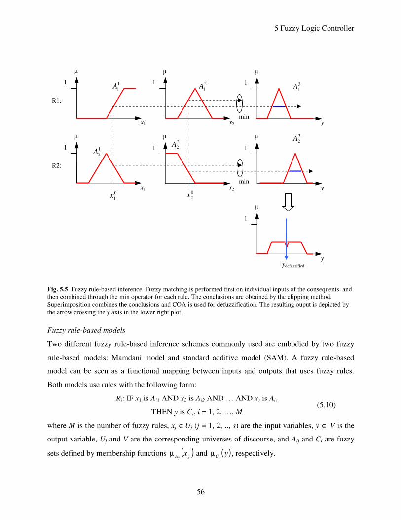
5 Fuzzy Logic Controller
56
Fig. 5.5 Fuzzy rule-based inference. Fuzzy matching is performed first on individual inputs of the consequents, and
then combined through the min operator for each rule. The conclusions are obtained by the clipping method.
Superimposition combines the conclusions and COA is used for defuzzification. The resulting ouput is depicted by
the arrow crossing the y axis in the lower right plot.
Fuzzy rule-based models
Two different fuzzy rule-based inference schemes commonly used are embodied by two fuzzy
rule-based models: Mamdani model and standard additive model (SAM). A fuzzy rule-based
model can be seen as a functional mapping between inputs and outputs that uses fuzzy rules.
Both models use rules with the following form:
Ri: IF x1 is Ai1 AND x2 is Ai2 AND … AND xs is Ais
THEN y is Ci, i = 1, 2, …, M (5.10)
where M is the number of fuzzy rules, xj ∈Uj (j = 1, 2, .., s) are the input variables, y ∈ V is the
output variable, Uj and V are the corresponding universes of discourse, and Aij and Ci are fuzzy
sets defined by membership functions ( )jA xij
µ and ( )yiCµ , respectively.
2
2A
x2
2
1A
x2
µ
x1
µ
1
1A 1
x1
1 1
2A
R1:
R2:
µ
1
µ
1
µ
y
3
1A 1
µ
y
3
2A
1
µ
y
1
v
min
min
0
1x 0
2x
ydefuzzified
5 Fuzzy Logic Controller
57
In the Mamdani model the result of the inference process can be obtained as follows. Given
inputs of the form:
x1 is A’1, x2 is A
’2, …, xs is A
’s
where A’1, A
’2, …, A
’s are fuzzy sets with universes of discourse U1, U2, …, Us, the conclusion of
rule Ri is:
( ) ( ) ( ) ( )yyyiii CisiiCiC µ∧∧∧∧=µ∧=µ ′ αααα L21 (5.11)
where ^ denotes the min operator, αi is the matching degree of rule Ri, and αij is the matching
degree between xj and Ri’s condition on xj:
( ) ( )( )jAjA
xij xx
ijj
j
µ∧µ= ′supα (5.12)
Eq. (5.11) is equivalent to the clipping inference method. The combination step to obtain the
fuzzy output C of the model is performed through superimposition:
( ) ( ) ( ) ( ){ }yyyyMCCCC ′′′ µµµ=µ ,,,max
21L (5.13)
The output can be defuzzified if necessary.
The SAM model is similar to the Mamdani but with the following differences: SAM assumes
crisp inputs, it uses scaling instead of clipping for inference, it applies addition instead of max
for combination, and it specifies COA as defuzzification technique. For a SAM model with two
inputs x1 and x2 that assume the crisp values 0
1x and 0
2x , respectively, the output of the model is:
( ) ( ) ( )
µ×µ×µ= ∑
i
CAA yxxCOAyiii
0
2
0
1 21 (5.14)
It can be proved that eq. (5.14) is equivalent to the following efficient expression:
( ) ( )( )
( ) ( )( )∑
∑
=
=
×µ×µ
××µ×µ
=M
i
iAA
M
i
iiAA
Bxx
gBxx
y
ii
ii
1
0
2
0
1
1
0
2
0
1
21
21
(5.15)
where:
( )∫ µ=y
Ci dyyBi
(5.16)
( )
( )∫
∫µ
µ=
yC
yC
i
dyy
ydyyg
i
i
(5.17)
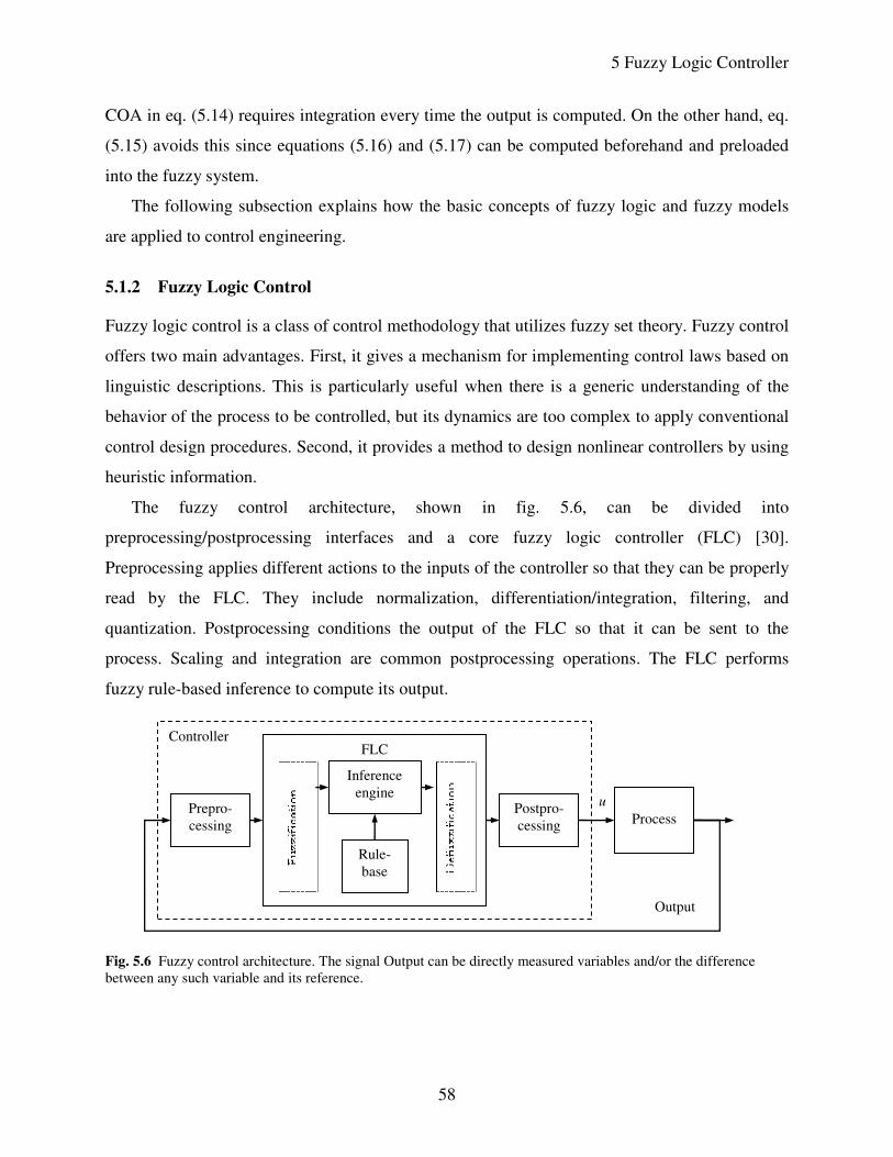
5 Fuzzy Logic Controller
58
COA in eq. (5.14) requires integration every time the output is computed. On the other hand, eq.
(5.15) avoids this since equations (5.16) and (5.17) can be computed beforehand and preloaded
into the fuzzy system.
The following subsection explains how the basic concepts of fuzzy logic and fuzzy models
are applied to control engineering.
5.1.2 Fuzzy Logic Control
Fuzzy logic control is a class of control methodology that utilizes fuzzy set theory. Fuzzy control
offers two main advantages. First, it gives a mechanism for implementing control laws based on
linguistic descriptions. This is particularly useful when there is a generic understanding of the
behavior of the process to be controlled, but its dynamics are too complex to apply conventional
control design procedures. Second, it provides a method to design nonlinear controllers by using
heuristic information.
The fuzzy control architecture, shown in fig. 5.6, can be divided into
preprocessing/postprocessing interfaces and a core fuzzy logic controller (FLC) [30].
Preprocessing applies different actions to the inputs of the controller so that they can be properly
read by the FLC. They include normalization, differentiation/integration, filtering, and
quantization. Postprocessing conditions the output of the FLC so that it can be sent to the
process. Scaling and integration are common postprocessing operations. The FLC performs
fuzzy rule-based inference to compute its output.
Fig. 5.6 Fuzzy control architecture. The signal Output can be directly measured variables and/or the difference
between any such variable and its reference.
Controller FLC
Prepro-
cessing
Inference
engine
Rule-
base
Postpro-
cessing
Process
u
Output
5 Fuzzy Logic Controller
59
The FLC has four main components: rule-base, inference engine, fuzzification interface, and
defuzzification interface [31]. The rule-base is the set of fuzzy if-then rules that encode the
control strategy. The inference engine executes the inference and combination steps of the fuzzy
rule-based inference process covered in subsection 5.1.1. Similarly, the fuzzification interface
performs the fuzzy matching step, and the defuzzification interface carries out the defuzzification
step.
As it was the case with membership functions, the rule-base can be derived from the
knowledge of the human operator of the process or the control engineer. An interview can be
done to the human operator, or the control engineer can rely on an intuitive model of the
behavior of the system obtained through experience: mathematical modeling, analysis,
experimentation, and design of control algorithms for the process.
The FLC can be implemented through any of the models outlined in the previous subsection:
Mamdani or SAM. These models are referred to as “standard fuzzy systems.” They rely on a
linguistic control strategy. Other models exist such as the Takagi-Sugeno-Kang (TSK) model
which is a “functional fuzzy system,” and is characterized by the use of functional consequents.
Functional fuzzy systems will no be covered here.
The control strategy encoded in the rule-base of the standard fuzzy control architecture has
the following general form:
IF OA1 is — AND OA2 is — AND …, THEN CA1 is — AND CA2 is — …
IF OA1 is — AND OA2 is — AND …, THEN CA1 is — AND CA2 is — …
…
where OA1, OA2, … are observable attributes of the given process and CA1, CA2, … are its
controllable attributes. Observable attributes can be directly measured variables, the difference
between such variables and their references, and/or filtered variables such as the derivative of
error. In fig. 5.6, they are the outputs of the preprocessing block. Controllable attributes are the
outputs of the FLC block in fig. 5.6.
The details of the specific design of the fuzzy controller proposed in this thesis are explained
in the next section.
5 Fuzzy Logic Controller
60
5.2 Design
The fuzzy logic controller designed for Icebreaker is a “standard fuzzy system” in which the
FLC core is implemented as the SAM fuzzy rule-based model. A standard fuzzy system was
selected because of the flexibility and simplicity of its design. In particular, control actions can
be established for specific slip scenarios, and the strategy can be defined via linguistic terms. The
SAM model was chosen because of its efficient implementation. This is crucial for planetary
rovers which usually have limited computing resources.
The architecture of the control system follows an incremental approach similar to the one
applied in the PI controller design. A block diagram representation of the system is shown in fig.
5.7. The fuzzy logic controller (FLC) acts in discrete time steps of period Ts. Its inputs are
normalized error en(t) and normalized change in error cen(t) which are defined as:
( ) ( )tente en = (5.18)
( ) ( ) ( )( )scen Ttetentce −−= (5.19)
where ne and nce are normalization factors. By computing change in error, the controller can use
the value to take preventive actions. The rules in the rule-base have the form:
IF en(t) is — AND cen(t) is —, THEN ∆un(t) is —
where ∆un(t) is the normalized output of the FLC. This output has to be denormalized, integrated,
and saturated to produce the control action u(t) sent to the process:
( ) ( ) ( )( )tudeTtutu nus ∆+−= ∆saturate (5.20)
where de∆u is the denormalization factor and saturate(·) is defined as:
( )
>
≤≤
<
=
20.0if20.0
20.00if
0if0
saturate
x
xx
x
x (5.21)
Signals yref, y, u, ∆u, and e are defined in the same way as they were defined in chapter 4: vehicle
slip reference, vehicle slip, commanded plow depth, commanded increment in plow depth, and
error in slip, respectively.
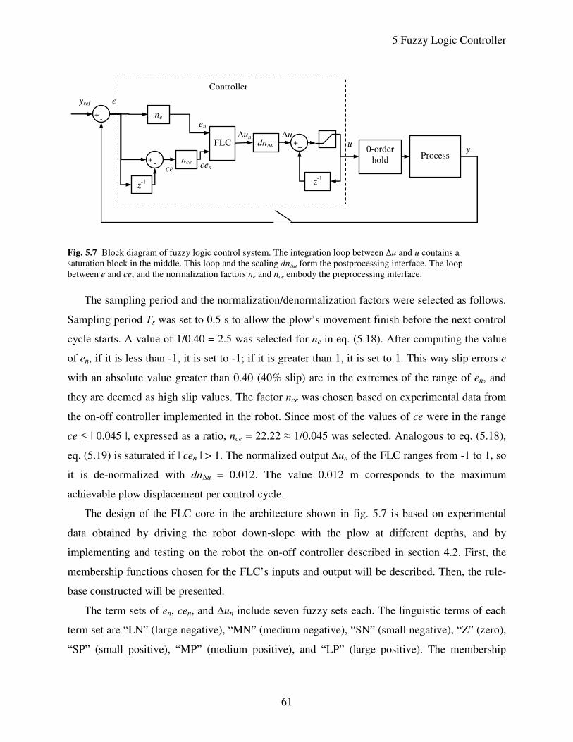
5 Fuzzy Logic Controller
61
Fig. 5.7 Block diagram of fuzzy logic control system. The integration loop between ∆u and u contains a
saturation block in the middle. This loop and the scaling dn∆u form the postprocessing interface. The loop
between e and ce, and the normalization factors ne and nce embody the preprocessing interface.
The sampling period and the normalization/denormalization factors were selected as follows.
Sampling period Ts was set to 0.5 s to allow the plow’s movement finish before the next control
cycle starts. A value of 1/0.40 = 2.5 was selected for ne in eq. (5.18). After computing the value
of en, if it is less than -1, it is set to -1; if it is greater than 1, it is set to 1. This way slip errors e
with an absolute value greater than 0.40 (40% slip) are in the extremes of the range of en, and
they are deemed as high slip values. The factor nce was chosen based on experimental data from
the on-off controller implemented in the robot. Since most of the values of ce were in the range
ce ≤ | 0.045 |, expressed as a ratio, nce = 22.22 ≈ 1/0.045 was selected. Analogous to eq. (5.18),
eq. (5.19) is saturated if | cen | > 1. The normalized output ∆un of the FLC ranges from -1 to 1, so
it is de-normalized with dn∆u = 0.012. The value 0.012 m corresponds to the maximum
achievable plow displacement per control cycle.
The design of the FLC core in the architecture shown in fig. 5.7 is based on experimental
data obtained by driving the robot down-slope with the plow at different depths, and by
implementing and testing on the robot the on-off controller described in section 4.2. First, the
membership functions chosen for the FLC’s inputs and output will be described. Then, the rule-
base constructed will be presented.
The term sets of en, cen, and ∆un include seven fuzzy sets each. The linguistic terms of each
term set are “LN” (large negative), “MN” (medium negative), “SN” (small negative), “Z” (zero),
“SP” (small positive), “MP” (medium positive), and “LP” (large positive). The membership
+ -
+ + 0-order
hold
Process
z-1
Controller
yref e
u ∆u
dn∆u ∆un
z-1
ne
nce + -
ce cen
en
FLC y
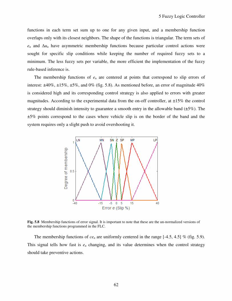
5 Fuzzy Logic Controller
62
functions in each term set sum up to one for any given input, and a membership function
overlaps only with its closest neighbors. The shape of the functions is triangular. The term sets of
en and ∆un have asymmetric membership functions because particular control actions were
sought for specific slip conditions while keeping the number of required fuzzy sets to a
minimum. The less fuzzy sets per variable, the more efficient the implementation of the fuzzy
rule-based inference is.
The membership functions of en are centered at points that correspond to slip errors of
interest: ±40%, ±15%, ±5%, and 0% (fig. 5.8). As mentioned before, an error of magnitude 40%
is considered high and its corresponding control strategy is also applied to errors with greater
magnitudes. According to the experimental data from the on-off controller, at ±15% the control
strategy should diminish intensity to guarantee a smooth entry in the allowable band (±5%). The
±5% points correspond to the cases where vehicle slip is on the border of the band and the
system requires only a slight push to avoid overshooting it.
Fig. 5.8 Membership functions of error signal. It is important to note that these are the un-normalized versions of
the membership functions programmed in the FLC.
The membership functions of cen are uniformly centered in the range [-4.5, 4.5] % (fig. 5.9).
This signal tells how fast is en changing, and its value determines when the control strategy
should take preventive actions.
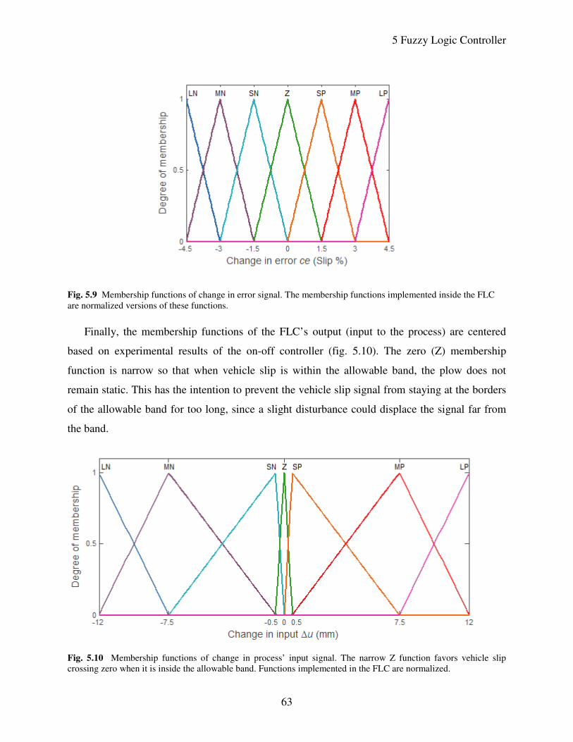
5 Fuzzy Logic Controller
63
Fig. 5.9 Membership functions of change in error signal. The membership functions implemented inside the FLC
are normalized versions of these functions.
Finally, the membership functions of the FLC’s output (input to the process) are centered
based on experimental results of the on-off controller (fig. 5.10). The zero (Z) membership
function is narrow so that when vehicle slip is within the allowable band, the plow does not
remain static. This has the intention to prevent the vehicle slip signal from staying at the borders
of the allowable band for too long, since a slight disturbance could displace the signal far from
the band.
Fig. 5.10 Membership functions of change in process’ input signal. The narrow Z function favors vehicle slip
crossing zero when it is inside the allowable band. Functions implemented in the FLC are normalized.
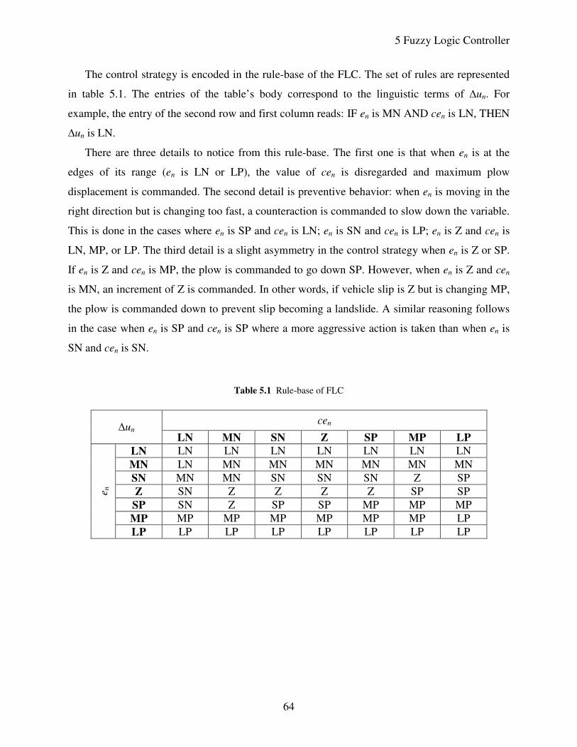
5 Fuzzy Logic Controller
64
The control strategy is encoded in the rule-base of the FLC. The set of rules are represented
in table 5.1. The entries of the table’s body correspond to the linguistic terms of ∆un. For
example, the entry of the second row and first column reads: IF en is MN AND cen is LN, THEN
∆un is LN.
There are three details to notice from this rule-base. The first one is that when en is at the
edges of its range (en is LN or LP), the value of cen is disregarded and maximum plow
displacement is commanded. The second detail is preventive behavior: when en is moving in the
right direction but is changing too fast, a counteraction is commanded to slow down the variable.
This is done in the cases where en is SP and cen is LN; en is SN and cen is LP; en is Z and cen is
LN, MP, or LP. The third detail is a slight asymmetry in the control strategy when en is Z or SP.
If en is Z and cen is MP, the plow is commanded to go down SP. However, when en is Z and cen
is MN, an increment of Z is commanded. In other words, if vehicle slip is Z but is changing MP,
the plow is commanded down to prevent slip becoming a landslide. A similar reasoning follows
in the case when en is SP and cen is SP where a more aggressive action is taken than when en is
SN and cen is SN.
Table 5.1 Rule-base of FLC
cen ∆un LN MN SN Z SP MP LP
LN LN LN LN LN LN LN LN
MN LN MN MN MN MN MN MN
SN MN MN SN SN SN Z SP
Z SN Z Z Z Z SP SP
SP SN Z SP SP MP MP MP
MP MP MP MP MP MP MP LP
e n
LP LP LP LP LP LP LP LP
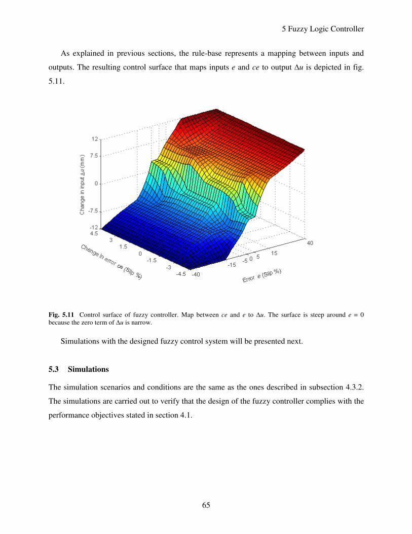
5 Fuzzy Logic Controller
65
As explained in previous sections, the rule-base represents a mapping between inputs and
outputs. The resulting control surface that maps inputs e and ce to output ∆u is depicted in fig.
5.11.
Fig. 5.11 Control surface of fuzzy controller. Map between ce and e to ∆u. The surface is steep around e = 0
because the zero term of ∆u is narrow.
Simulations with the designed fuzzy control system will be presented next.
5.3 Simulations
The simulation scenarios and conditions are the same as the ones described in subsection 4.3.2.
The simulations are carried out to verify that the design of the fuzzy controller complies with the
performance objectives stated in section 4.1.
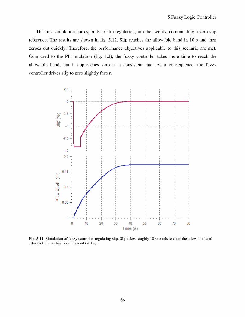
5 Fuzzy Logic Controller
66
The first simulation corresponds to slip regulation, in other words, commanding a zero slip
reference. The results are shown in fig. 5.12. Slip reaches the allowable band in 10 s and then
zeroes out quickly. Therefore, the performance objectives applicable to this scenario are met.
Compared to the PI simulation (fig. 4.2), the fuzzy controller takes more time to reach the
allowable band, but it approaches zero at a consistent rate. As a consequence, the fuzzy
controller drives slip to zero slightly faster.
Fig. 5.12 Simulation of fuzzy controller regulating slip. Slip takes roughly 10 seconds to enter the allowable band
after motion has been commanded (at 1 s).
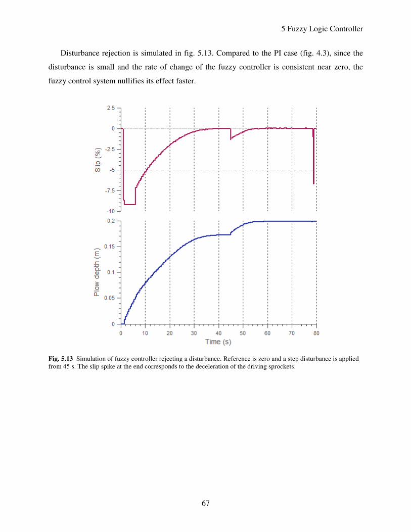
5 Fuzzy Logic Controller
67
Disturbance rejection is simulated in fig. 5.13. Compared to the PI case (fig. 4.3), since the
disturbance is small and the rate of change of the fuzzy controller is consistent near zero, the
fuzzy control system nullifies its effect faster.
Fig. 5.13 Simulation of fuzzy controller rejecting a disturbance. Reference is zero and a step disturbance is applied
from 45 s. The slip spike at the end corresponds to the deceleration of the driving sprockets.
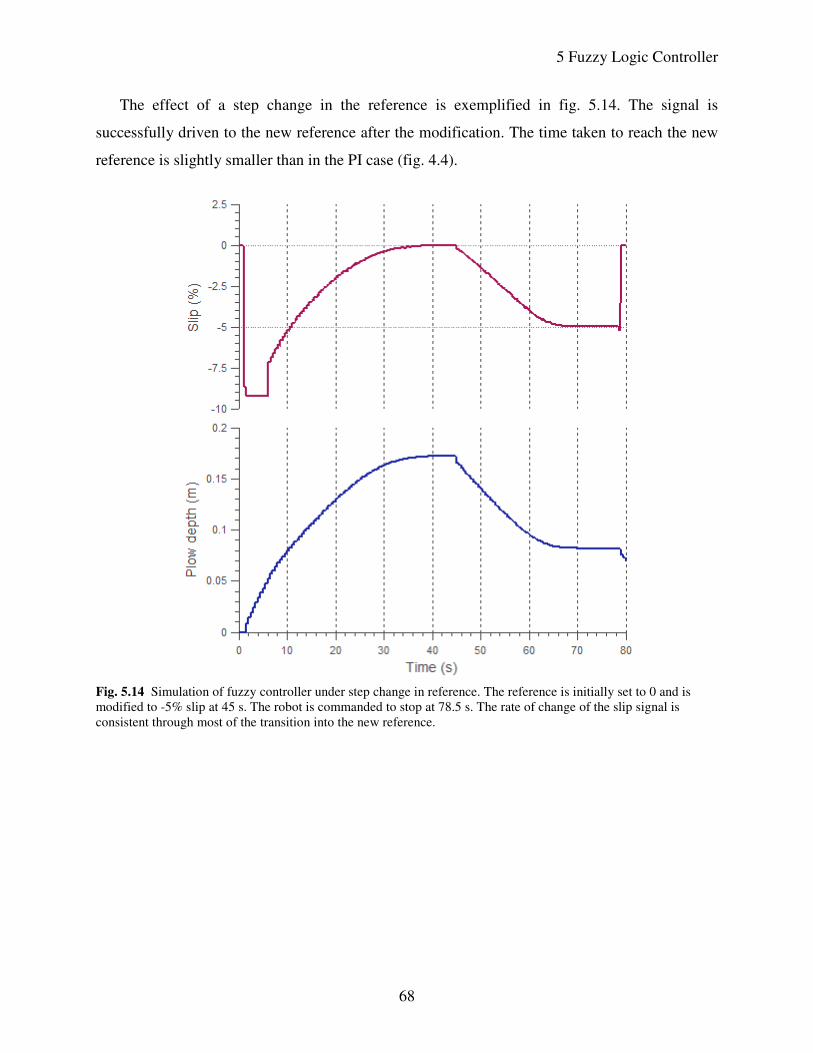
5 Fuzzy Logic Controller
68
The effect of a step change in the reference is exemplified in fig. 5.14. The signal is
successfully driven to the new reference after the modification. The time taken to reach the new
reference is slightly smaller than in the PI case (fig. 4.4).
Fig. 5.14 Simulation of fuzzy controller under step change in reference. The reference is initially set to 0 and is
modified to -5% slip at 45 s. The robot is commanded to stop at 78.5 s. The rate of change of the slip signal is
consistent through most of the transition into the new reference.
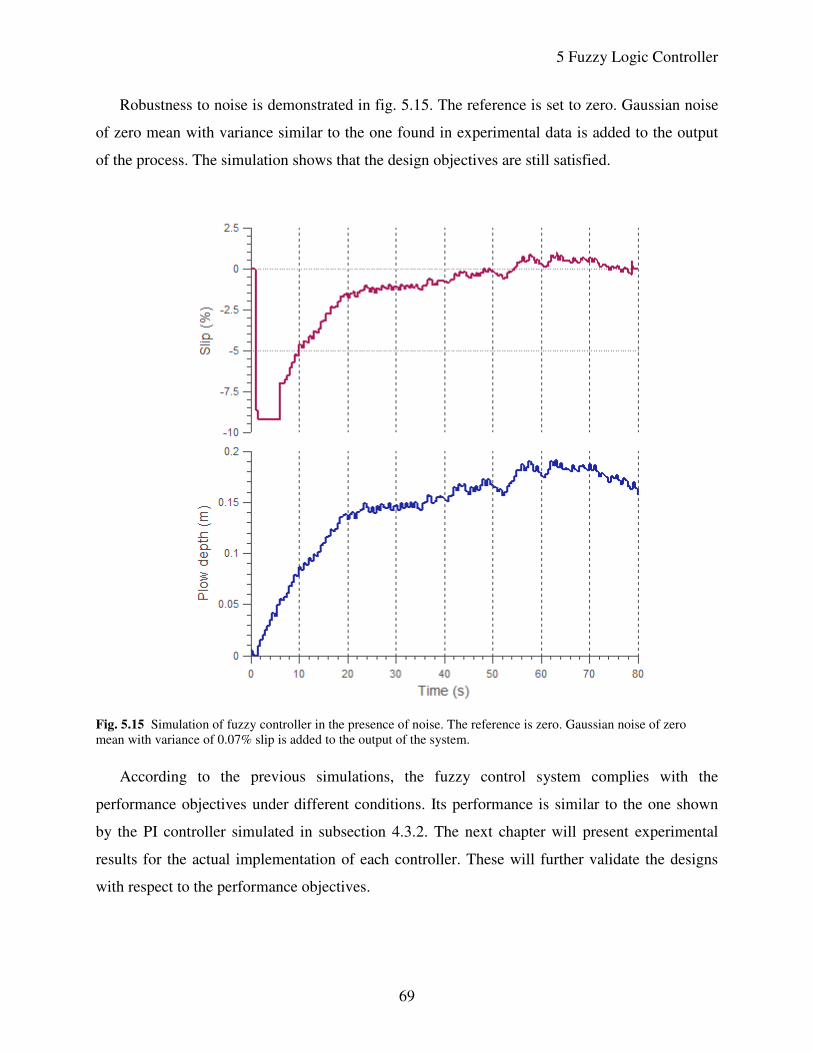
5 Fuzzy Logic Controller
69
Robustness to noise is demonstrated in fig. 5.15. The reference is set to zero. Gaussian noise
of zero mean with variance similar to the one found in experimental data is added to the output
of the process. The simulation shows that the design objectives are still satisfied.
Fig. 5.15 Simulation of fuzzy controller in the presence of noise. The reference is zero. Gaussian noise of zero
mean with variance of 0.07% slip is added to the output of the system.
According to the previous simulations, the fuzzy control system complies with the
performance objectives under different conditions. Its performance is similar to the one shown
by the PI controller simulated in subsection 4.3.2. The next chapter will present experimental
results for the actual implementation of each controller. These will further validate the designs
with respect to the performance objectives.
70
Chapter 6
Experimental Results
A series of experiments were carried out to corroborate that the performance objectives stated in
section 4.1 are met by the PI and fuzzy logic controller implementations, and to compare their
performance. In most of the tests, both controllers fully met the specifications, and only in very
few cases they were partially met. In general, it was found that the control system proposed is
able to arrest slip for different terrain grades and commanded speeds, to handle nonzero-slip
references under certain circumstances, and to cope with some deviations from the visual
odometry’s assumptions.
Some conventions were applied to the figures in this chapter. First, the robot’s driving
sprockets were already spinning at the commanded angular velocity in each plot. In other words,
the acceleration transitions of the sprockets when the rover is commanded to start moving and to
stop are not shown. Second, slip curves are plotted with small circles centered on the discrete
measurements. Third, the allowable band is depicted as dashed bold lines in the slip plots.
The chapter will explain first the experimental setup in which the tests were carried out. To
put into context the experimental results, an example of a descent without automatic slip control
will be presented afterwards. Then, the experiment with the on-off controller which served as a
slip-control proof of concept is shown. Finally, representative experiments that support the three
main results found are exposed and organized into: slip regulation (zero reference), slip control
of non-zero references, and slip control under violations of the visual odometry’s assumptions.
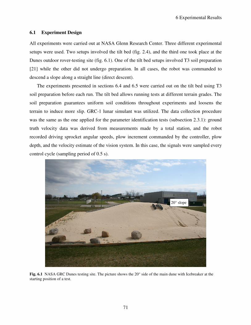
6 Experimental Results
71
6.1 Experiment Design
All experiments were carried out at NASA Glenn Research Center. Three different experimental
setups were used. Two setups involved the tilt bed (fig. 2.4), and the third one took place at the
Dunes outdoor rover-testing site (fig. 6.1). One of the tilt bed setups involved T3 soil preparation
[21] while the other did not undergo preparation. In all cases, the robot was commanded to
descend a slope along a straight line (direct descent).
The experiments presented in sections 6.4 and 6.5 were carried out on the tilt bed using T3
soil preparation before each run. The tilt bed allows running tests at different terrain grades. The
soil preparation guarantees uniform soil conditions throughout experiments and loosens the
terrain to induce more slip. GRC-1 lunar simulant was utilized. The data collection procedure
was the same as the one applied for the parameter identification tests (subsection 2.3.1): ground
truth velocity data was derived from measurements made by a total station, and the robot
recorded driving sprocket angular speeds, plow increment commanded by the controller, plow
depth, and the velocity estimate of the vision system. In this case, the signals were sampled every
control cycle (sampling period of 0.5 s).
Fig. 6.1 NASA GRC Dunes testing site. The picture shows the 20° side of the main dune with Icebreaker at the
starting position of a test.
20° slope
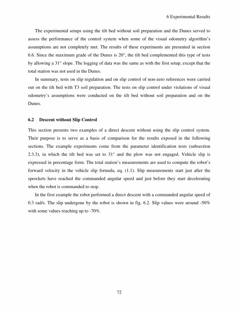
6 Experimental Results
72
The experimental setups using the tilt bed without soil preparation and the Dunes served to
assess the performance of the control system when some of the visual odometry algorithm’s
assumptions are not completely met. The results of these experiments are presented in section
6.6. Since the maximum grade of the Dunes is 20°, the tilt bed complemented this type of tests
by allowing a 31° slope. The logging of data was the same as with the first setup, except that the
total station was not used in the Dunes.
In summary, tests on slip regulation and on slip control of non-zero references were carried
out on the tilt bed with T3 soil preparation. The tests on slip control under violations of visual
odometry’s assumptions were conducted on the tilt bed without soil preparation and on the
Dunes.
6.2 Descent without Slip Control
This section presents two examples of a direct descent without using the slip control system.
Their purpose is to serve as a basis of comparison for the results exposed in the following
sections. The example experiments come from the parameter identification tests (subsection
2.3.3), in which the tilt bed was set to 31° and the plow was not engaged. Vehicle slip is
expressed in percentage form. The total station’s measurements are used to compute the robot’s
forward velocity in the vehicle slip formula, eq. (1.1). Slip measurements start just after the
sprockets have reached the commanded angular speed and just before they start decelerating
when the robot is commanded to stop.
In the first example the robot performed a direct descent with a commanded angular speed of
0.3 rad/s. The slip undergone by the robot is shown in fig. 6.2. Slip values were around -50%
with some values reaching up to -70%.
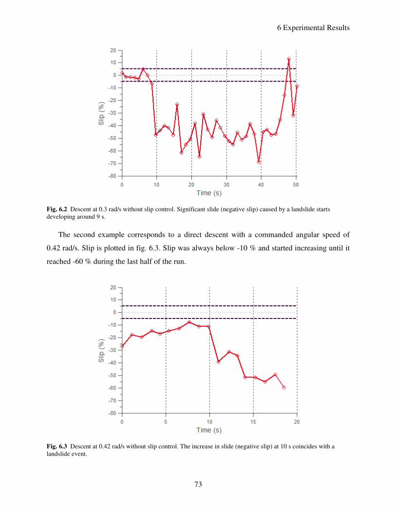
6 Experimental Results
73
Fig. 6.2 Descent at 0.3 rad/s without slip control. Significant slide (negative slip) caused by a landslide starts
developing around 9 s.
The second example corresponds to a direct descent with a commanded angular speed of
0.42 rad/s. Slip is plotted in fig. 6.3. Slip was always below -10 % and started increasing until it
reached -60 % during the last half of the run.
Fig. 6.3 Descent at 0.42 rad/s without slip control. The increase in slide (negative slip) at 10 s coincides with a
landslide event.
6 Experimental Results
74
Without slip control, the robot sled considerably, and slip values up to -70% appeared. The
next section covers an experiment that had the purpose of verifying if slip control for descending
steep slopes was feasible.
6.3 Slip-Control Proof of Concept: On-Off Controller
This experiment was performed during the first stages of the work presented in this thesis, and
had the intention of demonstrating that automatic slip control on extreme slopes was possible.
Since it was a proof of concept implementation, the forward velocity of the robot was computed
from measurements of the total station sent in real time to the robot, instead of using the vision
system. The details of the design of the on-off controller were presented in subsection 4.2.1. The
sampling time of the control system was set to 1 second. The experiment was carried out on the
tilt bed at 31° without soil preparation. Again, the soil was GRC-1. The robot was commanded
down slope driving the sprockets at 0.42 rad/s.
Vehicle slip and plow depth recorded during the experiment are shown in fig. 6.4. It can be
seen that even though at the beginning of the test a landslide occurred and caused slip values up
to -130%, the controller was able to overcome this and drove the slip toward the allowable band.
In the instances where the slip went out of the band, the controller took the signal inside again.
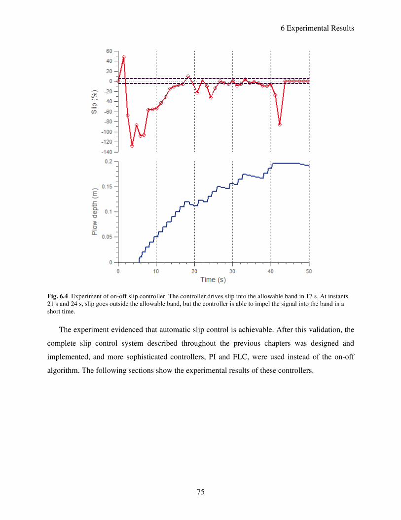
6 Experimental Results
75
Fig. 6.4 Experiment of on-off slip controller. The controller drives slip into the allowable band in 17 s. At instants
21 s and 24 s, slip goes outside the allowable band, but the controller is able to impel the signal into the band in a
short time.
The experiment evidenced that automatic slip control is achievable. After this validation, the
complete slip control system described throughout the previous chapters was designed and
implemented, and more sophisticated controllers, PI and FLC, were used instead of the on-off
algorithm. The following sections show the experimental results of these controllers.
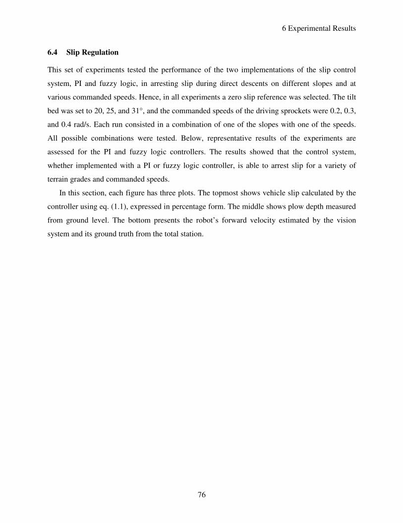
6 Experimental Results
76
6.4 Slip Regulation
This set of experiments tested the performance of the two implementations of the slip control
system, PI and fuzzy logic, in arresting slip during direct descents on different slopes and at
various commanded speeds. Hence, in all experiments a zero slip reference was selected. The tilt
bed was set to 20, 25, and 31°, and the commanded speeds of the driving sprockets were 0.2, 0.3,
and 0.4 rad/s. Each run consisted in a combination of one of the slopes with one of the speeds.
All possible combinations were tested. Below, representative results of the experiments are
assessed for the PI and fuzzy logic controllers. The results showed that the control system,
whether implemented with a PI or fuzzy logic controller, is able to arrest slip for a variety of
terrain grades and commanded speeds.
In this section, each figure has three plots. The topmost shows vehicle slip calculated by the
controller using eq. (1.1), expressed in percentage form. The middle shows plow depth measured
from ground level. The bottom presents the robot’s forward velocity estimated by the vision
system and its ground truth from the total station.
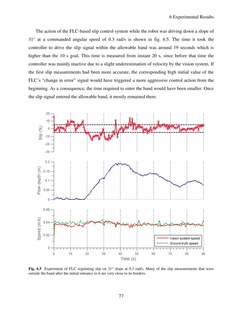
6 Experimental Results
77
The action of the FLC-based slip control system while the robot was driving down a slope of
31° at a commanded angular speed of 0.3 rad/s is shown in fig. 6.5. The time it took the
controller to drive the slip signal within the allowable band was around 19 seconds which is
higher than the 10 s goal. This time is measured from instant 20 s, since before that time the
controller was mainly inactive due to a slight underestimation of velocity by the vision system. If
the first slip measurements had been more accurate, the corresponding high initial value of the
FLC’s “change in error” signal would have triggered a more aggressive control action from the
beginning. As a consequence, the time required to enter the band would have been smaller. Once
the slip signal entered the allowable band, it mostly remained there.
Fig. 6.5 Experiment of FLC regulating slip on 31° slope at 0.3 rad/s. Many of the slip measurements that were
outside the band after the initial entrance to it are very close to its borders.
6 Experimental Results
78
An identical experiment was carried out using the PI-based slip control system. The results
are shown in fig. 6.6. The PI implementation took approximately 4.7 seconds to drive slip within
the allowable band. After the signal reached the band, very few points went outside the band, but
they were quickly brought back inside.
Fig. 6.6 Experiment of PI regulating slip on 31° slope at 0.3 rad/s. An initial high value of negative slip was
counteracted by a fast increase in plow depth.
For this pair of experiments, the PI was four times faster than the FLC with respect to the
first performance objective, the time taken to initially reach the allowable band. However, it is
important to keep in mind that in the FLC experiment there was a small underestimation of
velocity in the first seconds. The PI had fewer slip points above the band than the FLC, but
slightly more points below it. For both controllers, the points outside the band were near its
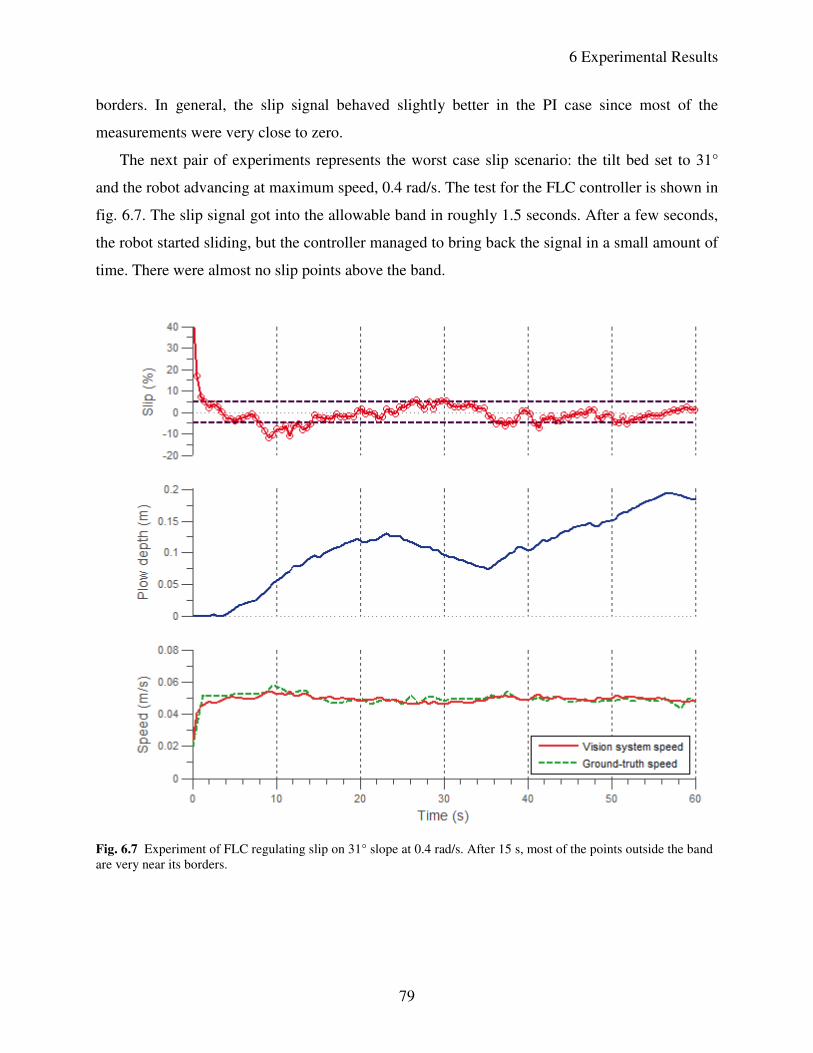
6 Experimental Results
79
borders. In general, the slip signal behaved slightly better in the PI case since most of the
measurements were very close to zero.
The next pair of experiments represents the worst case slip scenario: the tilt bed set to 31°
and the robot advancing at maximum speed, 0.4 rad/s. The test for the FLC controller is shown in
fig. 6.7. The slip signal got into the allowable band in roughly 1.5 seconds. After a few seconds,
the robot started sliding, but the controller managed to bring back the signal in a small amount of
time. There were almost no slip points above the band.
Fig. 6.7 Experiment of FLC regulating slip on 31° slope at 0.4 rad/s. After 15 s, most of the points outside the band
are very near its borders.
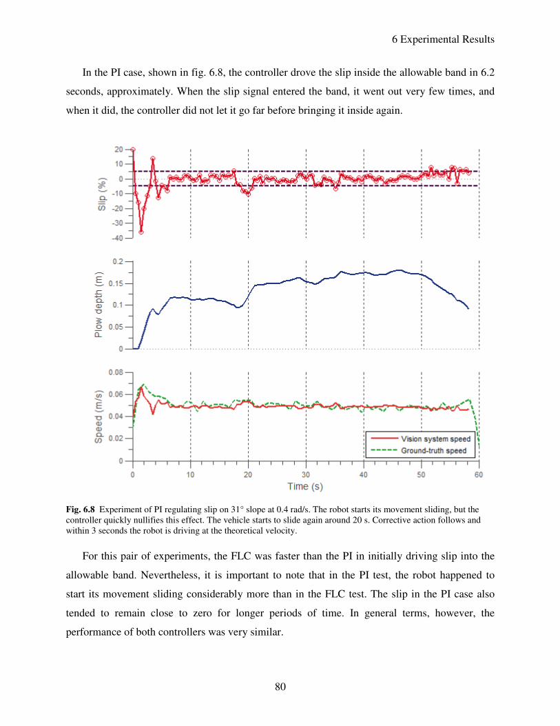
6 Experimental Results
80
In the PI case, shown in fig. 6.8, the controller drove the slip inside the allowable band in 6.2
seconds, approximately. When the slip signal entered the band, it went out very few times, and
when it did, the controller did not let it go far before bringing it inside again.
Fig. 6.8 Experiment of PI regulating slip on 31° slope at 0.4 rad/s. The robot starts its movement sliding, but the
controller quickly nullifies this effect. The vehicle starts to slide again around 20 s. Corrective action follows and
within 3 seconds the robot is driving at the theoretical velocity.
For this pair of experiments, the FLC was faster than the PI in initially driving slip into the
allowable band. Nevertheless, it is important to note that in the PI test, the robot happened to
start its movement sliding considerably more than in the FLC test. The slip in the PI case also
tended to remain close to zero for longer periods of time. In general terms, however, the
performance of both controllers was very similar.
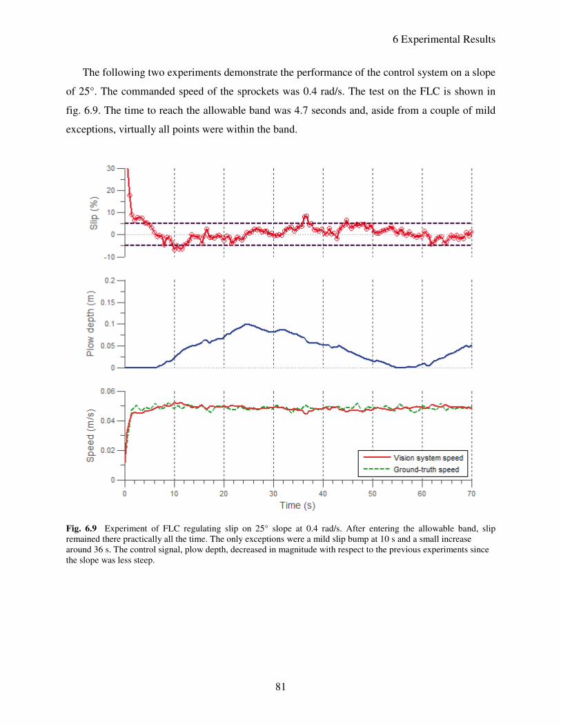
6 Experimental Results
81
The following two experiments demonstrate the performance of the control system on a slope
of 25°. The commanded speed of the sprockets was 0.4 rad/s. The test on the FLC is shown in
fig. 6.9. The time to reach the allowable band was 4.7 seconds and, aside from a couple of mild
exceptions, virtually all points were within the band.
Fig. 6.9 Experiment of FLC regulating slip on 25° slope at 0.4 rad/s. After entering the allowable band, slip
remained there practically all the time. The only exceptions were a mild slip bump at 10 s and a small increase
around 36 s. The control signal, plow depth, decreased in magnitude with respect to the previous experiments since
the slope was less steep.
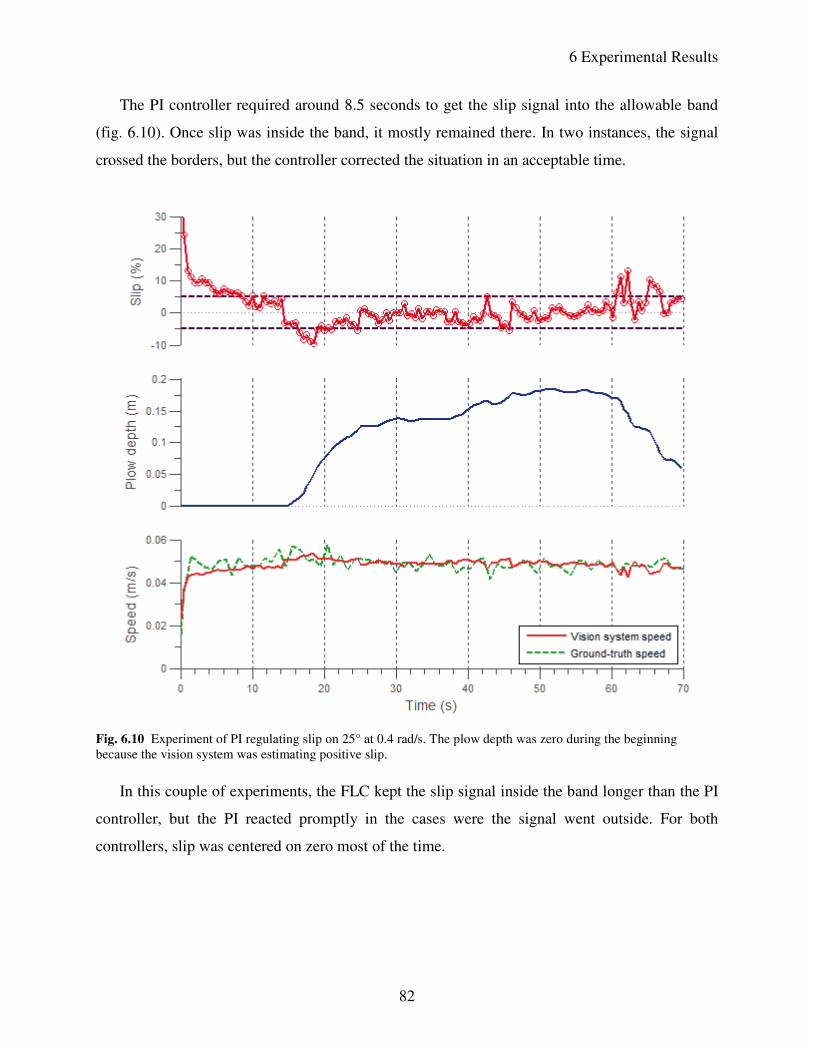
6 Experimental Results
82
The PI controller required around 8.5 seconds to get the slip signal into the allowable band
(fig. 6.10). Once slip was inside the band, it mostly remained there. In two instances, the signal
crossed the borders, but the controller corrected the situation in an acceptable time.
Fig. 6.10 Experiment of PI regulating slip on 25° at 0.4 rad/s. The plow depth was zero during the beginning
because the vision system was estimating positive slip.
In this couple of experiments, the FLC kept the slip signal inside the band longer than the PI
controller, but the PI reacted promptly in the cases were the signal went outside. For both
controllers, slip was centered on zero most of the time.
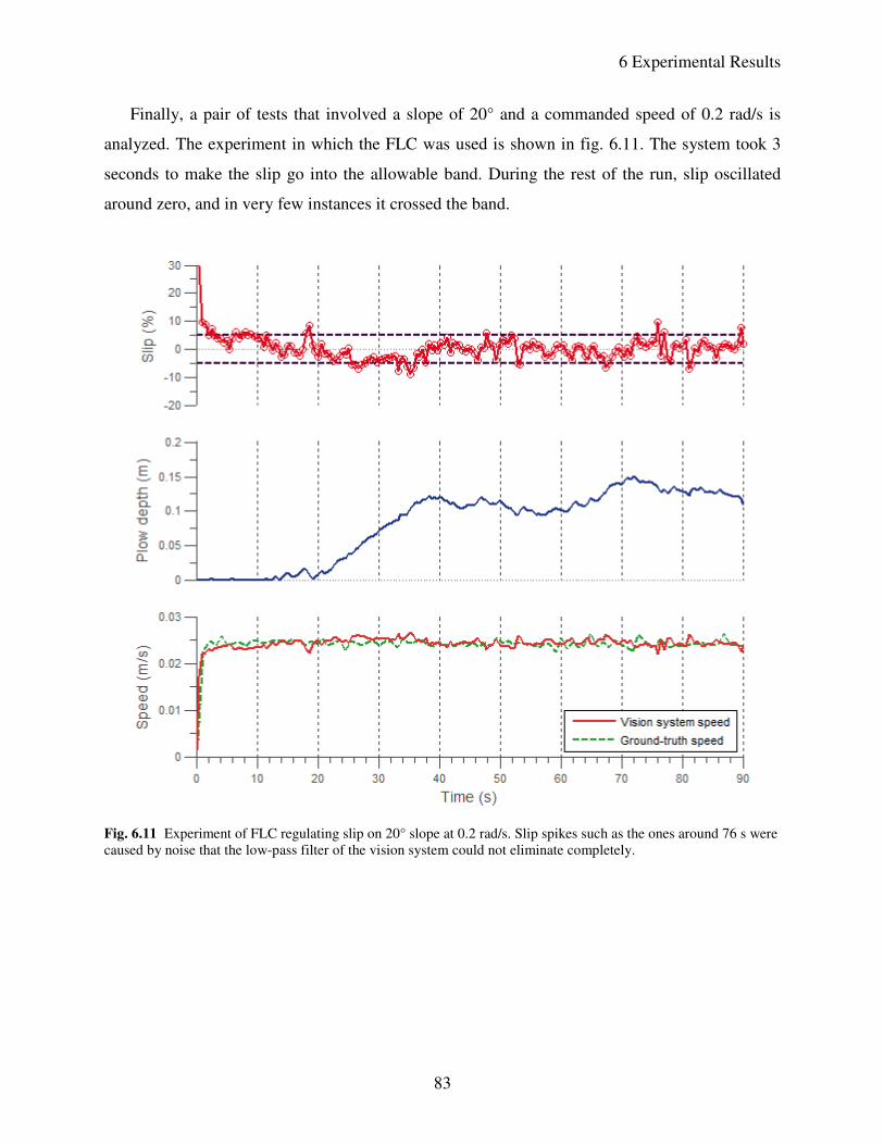
6 Experimental Results
83
Finally, a pair of tests that involved a slope of 20° and a commanded speed of 0.2 rad/s is
analyzed. The experiment in which the FLC was used is shown in fig. 6.11. The system took 3
seconds to make the slip go into the allowable band. During the rest of the run, slip oscillated
around zero, and in very few instances it crossed the band.
Fig. 6.11 Experiment of FLC regulating slip on 20° slope at 0.2 rad/s. Slip spikes such as the ones around 76 s were
caused by noise that the low-pass filter of the vision system could not eliminate completely.
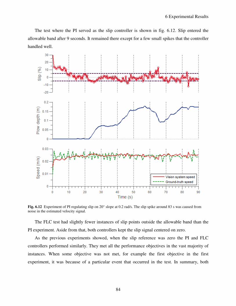
6 Experimental Results
84
The test where the PI served as the slip controller is shown in fig. 6.12. Slip entered the
allowable band after 9 seconds. It remained there except for a few small spikes that the controller
handled well.
Fig. 6.12 Experiment of PI regulating slip on 20° slope at 0.2 rad/s. The slip spike around 83 s was caused from
noise in the estimated velocity signal.
The FLC test had slightly fewer instances of slip points outside the allowable band than the
PI experiment. Aside from that, both controllers kept the slip signal centered on zero.
As the previous experiments showed, when the slip reference was zero the PI and FLC
controllers performed similarly. They met all the performance objectives in the vast majority of
instances. When some objective was not met, for example the first objective in the first
experiment, it was because of a particular event that occurred in the test. In summary, both
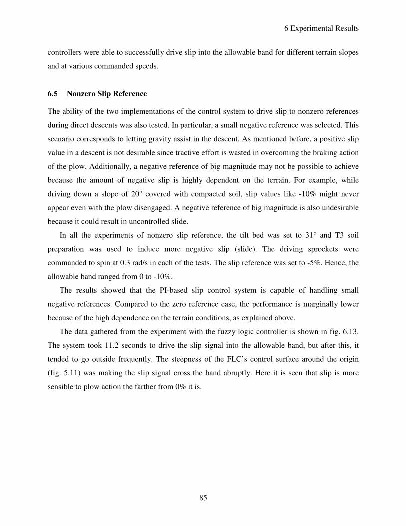
6 Experimental Results
85
controllers were able to successfully drive slip into the allowable band for different terrain slopes
and at various commanded speeds.
6.5 Nonzero Slip Reference
The ability of the two implementations of the control system to drive slip to nonzero references
during direct descents was also tested. In particular, a small negative reference was selected. This
scenario corresponds to letting gravity assist in the descent. As mentioned before, a positive slip
value in a descent is not desirable since tractive effort is wasted in overcoming the braking action
of the plow. Additionally, a negative reference of big magnitude may not be possible to achieve
because the amount of negative slip is highly dependent on the terrain. For example, while
driving down a slope of 20° covered with compacted soil, slip values like -10% might never
appear even with the plow disengaged. A negative reference of big magnitude is also undesirable
because it could result in uncontrolled slide.
In all the experiments of nonzero slip reference, the tilt bed was set to 31° and T3 soil
preparation was used to induce more negative slip (slide). The driving sprockets were
commanded to spin at 0.3 rad/s in each of the tests. The slip reference was set to -5%. Hence, the
allowable band ranged from 0 to -10%.
The results showed that the PI-based slip control system is capable of handling small
negative references. Compared to the zero reference case, the performance is marginally lower
because of the high dependence on the terrain conditions, as explained above.
The data gathered from the experiment with the fuzzy logic controller is shown in fig. 6.13.
The system took 11.2 seconds to drive the slip signal into the allowable band, but after this, it
tended to go outside frequently. The steepness of the FLC’s control surface around the origin
(fig. 5.11) was making the slip signal cross the band abruptly. Here it is seen that slip is more
sensible to plow action the farther from 0% it is.
6 Experimental Results
86
Fig. 6.13 Nonzero slip reference experiment with FLC. The shape of the FLC’s control surface around the origin
causes the slip signal to cross throughout the band in one sampling period (see instants 41 s and 57 s). The effect of
the surface’s shape is also reflected in the numerous small peaks in the plow depth signal.
The results of an analogous experiment with the PI controller are shown in fig. 6.14. The
performance objectives were met. The system took the slip into the allowable band in 5 seconds,
and from there on, it mostly remained inside the band. At the middle of the test there was a
considerable increase in slide, but the controller was able to bring the signal into the allowable
band in a short time. It can also be noted that the signal remained on the upper border of the band
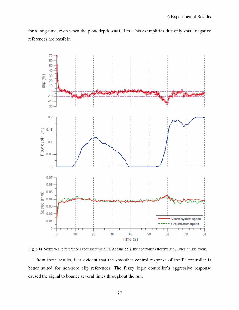
6 Experimental Results
87
for a long time, even when the plow depth was 0.0 m. This exemplifies that only small negative
references are feasible.
Fig. 6.14 Nonzero slip reference experiment with PI. At time 55 s, the controller effectively nullifies a slide event.
From these results, it is evident that the smoother control response of the PI controller is
better suited for non-zero slip references. The fuzzy logic controller’s aggressive response
caused the signal to bounce several times throughout the run.
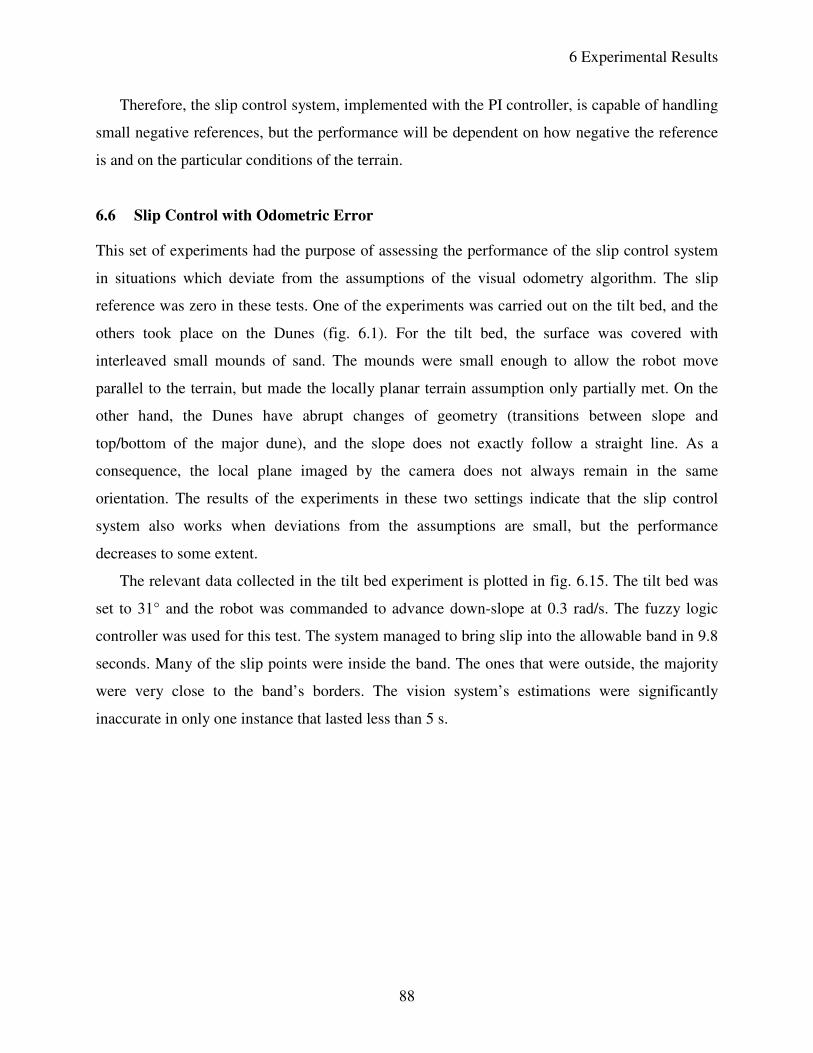
6 Experimental Results
88
Therefore, the slip control system, implemented with the PI controller, is capable of handling
small negative references, but the performance will be dependent on how negative the reference
is and on the particular conditions of the terrain.
6.6 Slip Control with Odometric Error
This set of experiments had the purpose of assessing the performance of the slip control system
in situations which deviate from the assumptions of the visual odometry algorithm. The slip
reference was zero in these tests. One of the experiments was carried out on the tilt bed, and the
others took place on the Dunes (fig. 6.1). For the tilt bed, the surface was covered with
interleaved small mounds of sand. The mounds were small enough to allow the robot move
parallel to the terrain, but made the locally planar terrain assumption only partially met. On the
other hand, the Dunes have abrupt changes of geometry (transitions between slope and
top/bottom of the major dune), and the slope does not exactly follow a straight line. As a
consequence, the local plane imaged by the camera does not always remain in the same
orientation. The results of the experiments in these two settings indicate that the slip control
system also works when deviations from the assumptions are small, but the performance
decreases to some extent.
The relevant data collected in the tilt bed experiment is plotted in fig. 6.15. The tilt bed was
set to 31° and the robot was commanded to advance down-slope at 0.3 rad/s. The fuzzy logic
controller was used for this test. The system managed to bring slip into the allowable band in 9.8
seconds. Many of the slip points were inside the band. The ones that were outside, the majority
were very close to the band’s borders. The vision system’s estimations were significantly
inaccurate in only one instance that lasted less than 5 s.
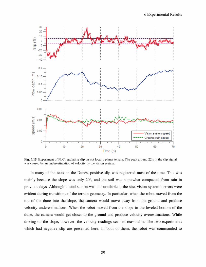
6 Experimental Results
89
Fig. 6.15 Experiment of FLC regulating slip on not locally planar terrain. The peak around 22 s in the slip signal
was caused by an underestimation of velocity by the vision system.
In many of the tests on the Dunes, positive slip was registered most of the time. This was
mainly because the slope was only 20°, and the soil was somewhat compacted from rain in
previous days. Although a total station was not available at the site, vision system’s errors were
evident during transitions of the terrain geometry. In particular, when the robot moved from the
top of the dune into the slope, the camera would move away from the ground and produce
velocity underestimations. When the robot moved from the slope to the leveled bottom of the
dune, the camera would get closer to the ground and produce velocity overestimations. While
driving on the slope, however, the velocity readings seemed reasonable. The two experiments
which had negative slip are presented here. In both of them, the robot was commanded to
6 Experimental Results
90
perform a direct descent at 0.4 rad/s. One of the tests used the FLC controller and the other the
PI. The data was logged while the robot was driving on the slope.
The results of the experiment with the FLC are shown in fig. 6.16. The controller drove the
slip into the band in 7 seconds. Many of the slip points were inside the band. Aside from an
interval of time in which the robot slipped with the plow disengaged, most of the points outside
the band were close to its borders.
Fig. 6.16 Experiment of FLC in Dunes. Between 22 and 35 s, the robot was slipping even though the plow was
disengaged, which means the event was closely related to local terrain conditions. It took around 10 seconds for the
slip to enter the allowable band again.
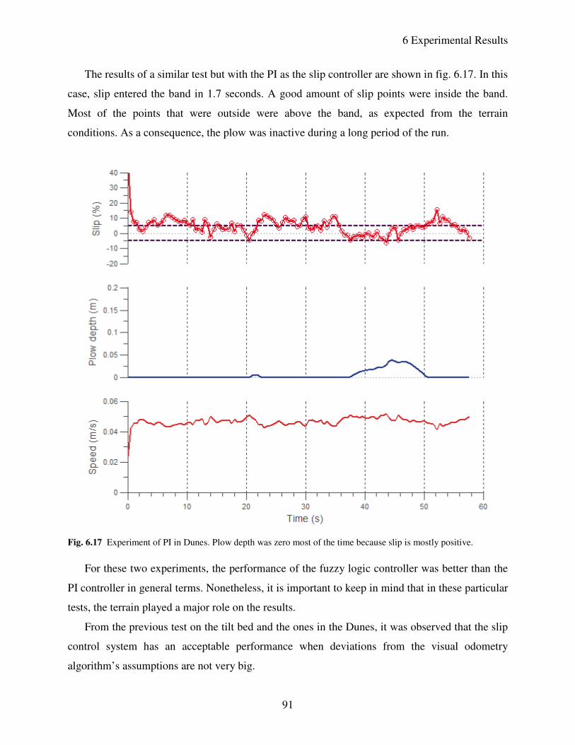
6 Experimental Results
91
The results of a similar test but with the PI as the slip controller are shown in fig. 6.17. In this
case, slip entered the band in 1.7 seconds. A good amount of slip points were inside the band.
Most of the points that were outside were above the band, as expected from the terrain
conditions. As a consequence, the plow was inactive during a long period of the run.
Fig. 6.17 Experiment of PI in Dunes. Plow depth was zero most of the time because slip is mostly positive.
For these two experiments, the performance of the fuzzy logic controller was better than the
PI controller in general terms. Nonetheless, it is important to keep in mind that in these particular
tests, the terrain played a major role on the results.
From the previous test on the tilt bed and the ones in the Dunes, it was observed that the slip
control system has an acceptable performance when deviations from the visual odometry
algorithm’s assumptions are not very big.

92
Chapter 7
Discussion
This chapter first gives the conclusions drawn from the work that has been presented. Then, it
exposes the contributions brought by this research. Finally, it outlines possible paths for further
work.
7.1 Conclusions
Several inferences can be made from the development of the slip control system presented in this
thesis: the system successfully controls slip during very steep descents; its two implementations
are comparable in terms of performance, but they differ in their design procedures; its vision
component does have a significant effect on performance; and the control action for nonzero
references should be smooth.
As chapter 6 demonstrates, the problem stated in section 1.2 has been solved: an automatic
system for controlling slip of a plowing-capable rover during direct descent on extreme slopes
has been developed. It rapidly drives the slip to the reference, and keeps the value close to the
setpoint. The experiments also showed that the system is able to handle a variety of terrain
grades and commanded speeds.
The two implementations of the system, classical control (PI) and fuzzy logic control,
performed similarly well; the difference lies mainly in their design procedures. The simplicity of
the PI controller comes at the cost of fewer options for fine-tuning its behavior. For example, it is
difficult to tune the controller constants so that for all possible inputs, the output is less than the
maximum allowable plow displacement per control cycle. On the other hand, the fuzzy logic
7 Discussion
93
controller offers increased flexibility at the cost of more design decisions to make. Nevertheless,
fuzzy logic streamlines the high level design with the linguistic formulation of the control law. In
this way, the control engineer can easily encode into the control strategy informal knowledge of
a process that has difficult to model dynamics.
Although the performance did not change much between the two slip controllers, the
accuracy of the vision system component has an important impact on it. This comes from the fact
that slip, eq. (1.1), is directly calculated from the vision system’s velocity estimate. So changes
of height between the camera and the ground, that can produce considerable velocity error, might
diminish the performance of the control system. However, if the deviations from the visual
odometry’s assumptions are small, as was the case with the terrain’s local flatness, the control
system is robust to the resulting inaccuracies.
Lastly, it was also observed that nonzero slip references require a smoother control action
when the signal is near the setpoint than zero references do. Such requirement was met by the PI
design. For the FLC case, the slip values bounced across the allowable band when the reference
was -5% (fig. 6.13). Additionally, the value of a feasible reference depends on terrain conditions.
For instance, the reference range [0, -5] % is acceptable for a slope of 31° covered with loose soil
(fig. 6.14). A more negative reference for this setting would not be possible since there are cases
when the slip values are near zero even though the plow depth is zero (e.g. 40 s – 50 s of fig.
6.14).
In summary, the research problem explained in the introduction of the thesis was solved, the
two implementations of the control system perform comparably while their design is different,
the vision system’s accuracy has an important impact on the performance of the control system,
and the control action for nonzero references should be smooth near the target.
7.2 Summary of Contributions
The main contributions of this thesis are the development of the first automatic system that uses
plowing for controlling rover’s slip during descent on extreme slopes, the realization of slip
control without affecting the commanded velocity of the vehicle, and the first demonstration of
fuzzy logic applied to slip control for extreme slope descents.
Foremost, this thesis developed the first system that automatically controls rover slip through
plowing while descending extreme slopes. Other research has dealt with slip control for rovers
7 Discussion
94
driving on uneven horizontal terrain [16] or simple motion strategies for steep descents [7]. The
automatic system proposed in this thesis directly controls the slip undergone by rovers
descending slopes of up to 31° covered with loose sand. This expands current rover mobility
capabilities, and represents a step forward toward the exploration of craters in other planetary
bodies.
The second contribution is the realization of slip control without affecting the commanded
velocity of the rover. Existing slip control systems employ wheel torques or speeds as controlled
variables. As a consequence, the commanded velocity of the robot has to be changed during the
control action. Icebreaker’s plow provides an additional degree of freedom through which slip
control can be executed independently of the commands sent to the running gear. This, for
example, facilitates correction of odometric errors. The control system, as shown in chapter 6,
minimizes the frequency and duration of slide events, and because it does not modify the
commanded velocity of the robot, it would only be necessary to keep track of slip when such
events happen.
Thirdly, this thesis demonstrated the first application of fuzzy logic to slip control for
extreme slope descents. This expands the myriad of successful applications of the fuzzy
methodology which include anti-lock braking systems (ABS), traction control systems (TCS),
and locomotive wheel slip control.
Therefore, the work presented in this thesis has a positive impact in the field of robotics and
controls by developing the first slip control system based on plowing for descent of extreme
slopes, by providing the capability of controlling slip independently of commanded speeds, and
by expanding the existing applications of fuzzy logic.
7.3 Future Research
The work presented in this thesis can be further extended in four different areas: slip estimation,
terramechanics of slope traversal, descent strategies, and slip controller.
The first opportunity for further research is the improvement of slip estimation on rough
terrain. Although velocity estimation was accurate most of the time, considerable errors were
observed in experiments that deviated enough from the visual odometry’s assumptions. One
example is the change of height between the camera and the ground. Possible solutions include
the use of a camera with telecentric lens. This way, the magnification of an imaged object is the
7 Discussion
95
same independently of its distance. Another option could be the use of a filter to enhance visual
odometry estimates. A sliding mode observer or a particle filter seem good choices because they
do not require the linearizations made by an EKF.
Also, a deep study in the terramechanics of slope traversal is required. The research on
fundamental terramechanics of slope traversal is scarce. As a consequence, the dynamics of
phenomena such as landslides are still not well understood. A sufficiently accurate mathematical
description of such interactions could be exploited by model-based control algorithms (fuzzy and
non-fuzzy) in controlling slip.
The third direction of future research is to expand slip control to other types of descents. This
thesis studied direct descents, but there are other strategies to descend slopes such as a “zig-zag”
approach. Performing other descent methods would require the control of the complete set of slip
parameters: longitudinal slip of each track and slip angle of the rover.
The fourth area of improvement is the slip controller itself. The experimental results of the
fuzzy controller were good, except for the nonzero slip reference tests where the PI performed
better. Since a fuzzy logic controller is a universal function approximator, its control surface can
be shaped around the origin so that it matches the PI. Then, nonlinearities in the surface can be
shaped away from the origin as required.
As it can be seen, the work presented in this thesis can be extended by improving the slip
estimation on rough terrain, studying the fundamental terramechanics of slope traversal,
expanding slip control to other types of descents, and incorporating the strengths of the PI
controller into the fuzzy logic controller.
96
References
[1] J. Ziglar, “Rover configuration for exploring lunar craters,” M.S. thesis, Robotics Inst.,
Carnegie Mellon Univ., Pittsburgh, PA, 2007.
[2] D. Kohanbash, “Plowing for rover control on extreme slopes,” M.S. thesis, Robotics Inst.,
Carnegie Mellon Univ., Pittsburgh, PA, 2011.
[3] J. Y. Wong, Theory of Ground Vehicles, 3rd ed. New York: John Wiley & Sons, 2001.
[4] M. G. Bekker, Theory of Land Locomotion. Ann Arbor, MI: Univ. of Michigan Press,
1956.
[5] T. Muro and J. O’Brien, Terramechanics Land Locomotion Mechanics. Lisse,
Netherlands: A. A. Balkema Publishers, 2004.
[6] G. Ishigami, A. Miwa, K. Nagatani, and K. Yoshida, “Terramechanics-based analysis on
slope traversability for a planetary exploration rover,” in Proc. 25th Int. Symp. Space
Technology and Science, Kanazawa, Japan, 2006, pp. 1025–1030.
[7] W. D. Huang, J. S. Bao, and Y. S. Xu, “Terramechanics model and motion control
strategy simulation for down-slope travel of a lunar rover,” Applied Mechanics and
Materials, vol. 215–216, pp. 1291–1297, Nov. 2012.
[8] L. Ojeda and D. Cruz, “Current-based slippage detection and odometry correction for
mobile robots and planetary rovers,” IEEE Trans. Robot., vol. 22, no. 2, pp. 366–378,
2006.
[9] M. Maimone, Y. Cheng, and L. Matthies, “Two years of visual odometry on the Mars
exploration rovers,” Journal of Field Robotics, vol. 24, no. 3, pp. 169–186, Mar. 2007.
[10] A. E. Johnson, S. B. Goldberg, Y. Cheng, and L. H. Matthies, “Robust and efficient stereo
feature tracking for visual odometry,” in 2008 IEEE Int. Conf. Robotics and Automation,
Pasadena, CA, 2008, pp. 39–46.
[11] N. Seegmiller and D. Wettergreen, “Optical flow odometry with robustness to self-
shadowing,” in 2011 IEEE/RSJ Int. Conf. Intelligent Robots and Systems, San Francisco,
CA, 2011, pp. 613–618.
[12] A. T. Le, D. C. Rye, and H. F. Durrant-White, “Estimation of track-soil interactions for
autonomous tracked vehicles,” in Proc. 1997 IEEE Int. Conf. Robotics and Automation,
Albuquerque, NM, 1997, pp. 1388–1393.
[13] T. M. Dar and R. G. Longoria, “Slip estimation for small-scale robotic tracked vehicles,”
in 2010 American Control Conf., Baltimore, MD, 2010, pp. 6816–6821.
[14] P. Saeedi et al., “An autonomous excavator with vision-based track slippage control,”
IEEE Trans. Control Systems Technology, vol. 13, no. 1, pp. 67–84, Jan. 2005.
[15] G. Ishigami, K. Nagatani, and K. Yoshida, “Slope traversal experiments with slip
compensation control for lunar/planertary exploration rover,” in 2008 IEEE Int. Conf.
Robotics and Automation, Pasadena, CA, 2008, pp. 2295–2300.
[16] K. Yoshida and H. Hamano, “Motion dynamics and control of a planetary rover with slip-
based traction model,” in Proc. 2002 IEEE Int. Conf. Robotics and Automation,
Washington, DC, 2002, pp. 3155–3160.
97
[17] U. S. NASA, “Walls of lunar crater may hold patchy ice, LRO radar finds,” 2012.
[Online]. Available: http://www.nasa.gov/mission_pages/LRO/news/shackleton-ice.html.
[Accessed: 21-Apr-2013].
[18] G. H. Heiken, D. T. Vaniman, and B. M. French, Lunar Sourcebook A User’s Guide to the
Moon. New York, NY: Cambridge Univ. Press, 1991.
[19] U. S. NASA, “Mount Sharp inside Gale Crater, Mars,” 2012. [Online]. Available:
http://www.nasa.gov/mission_pages/msl/multimedia/pia15292.html. [Accessed: 21-Apr-
2013].
[20] H. a. Oravec, X. Zeng, and V. M. Asnani, “Design and characterization of GRC-1: A soil
for lunar terramechanics testing in Earth-ambient conditions,” Journal of Terramechanics,
vol. 47, no. 6, pp. 361–377, Dec. 2010.
[21] A. C. Woodward, “Experimental analysis of the effects of the variation of drawbar pull
test parameters for exploration vehicles on GRC-1 lunar soil simulant,” M.S. thesis, Mech.
Eng. Dept., Virginia Polytechnic Inst. and State Univ., 2011.
[22] P. H. Menold, R. K. Pearson, and F. Allgower, “Online outlier detection and removal,” in
Proc. 7th Mediterranean Conf. Control and Automation, Haifa, Israel, 1999, pp. 1110–
1133.
[23] B. K. P. Horn and B. G. Schunck, “Determining optical flow,” Artificial Intelligence, vol.
17, no. 1–3, pp. 185–203, Aug. 1981.
[24] J. Campbell, R. Sukthankar, and I. Nourbakhsh, “Techniques for evaluating optical flow
for visual odometry in extreme terrain,” in 2004 IEEE/RSJ Int. Conf. Intelligent Robots
and Systems, Sendai, Japan, 2004, pp. 3704–3711.
[25] L.-P. Morency and R. Gupta, “Robust real-time egomotion from stereo images,” in Proc.
2003 Int. Conf. Image Processing, Barcelona, Spain, 2003, pp. 719–722.
[26] X. Song, Z. Song, L. D. Seneviratne, and K. Althoefer, “Optical flow-based slip and
velocity estimation technique for unmanned skid-steered vehicles,” 2008 IEEE/RSJ
Int.Conf. Intelligent Robots and Systems, pp. 101–106, Sep. 2008.
[27] J. Challis, “A procedure for determining rigid body transformation parameters,” Journal
of Biomechanics, vol. 28, no. 6, pp. 733–737, 1995.
[28] D. E. Seborg, D. A. Mellichamp, and F. E. Thomas, Process Dynamics and Control, 1st
ed. Somerset, NJ: John Wiley & Sons, 1986.
[29] J. Yen and R. Langari, Fuzzy Logic Intelligence, Control, and Information. Upper Saddle
River, NJ: Prentice Hall, 1999.
[30] J. Jantzen, “Design of fuzzy controllers,” Dept. Automation, Technical Univ. of Denmark,
Lyngby, Denmark, Tech. Rep. 98-E, 1998.