Small Transmitting Loop Antennas—A different perspective

on determining Q and efficiency

Over the past several decades there have been numerous published articles that describe the

construction and testing of small transmitting loop antennas. 'Small', in this context, refers to an

antenna that has a circumference that is less than about 0.1 wavelength. In this article I want to focus

more on evaluation of the performance of the antenna and little on the construction aspects. I will rely

on both models and measurements on a simple loop antenna. To my knowledge, there have been no

articles that describe the method of determining the Q of the antenna as presented herein. Note also,

that I do not attempt to cover electromagnetic modeling using such tools as NEC and EZNEC.

References at the end of this article describe construction methods, NEC models, etc.

The purpose of this paper:

-Describe the electrical behavior of a small transmitting loop antenna near the tuned frequency using an

electrical circuit analogue.

-Provide guidance in tuning the antenna for an impedance match to a coaxial transmission line.

-Describe a measurement for determining the 'Q' of the antenna system.

-Estimate the efficiency of the antenna (fraction of the applied power that is radiated to the far field)

based on measured Q.

-Compare model data with data obtained from measurements.

Assumptions-

-The circumference of the loop is small compared to wavelength (Current is essentially constant around

the loop).

-Coax is connected to a small coupling loop that is magnetically coupled to the main loop. The

analysis should also apply to a “delta” or “gamma” match.

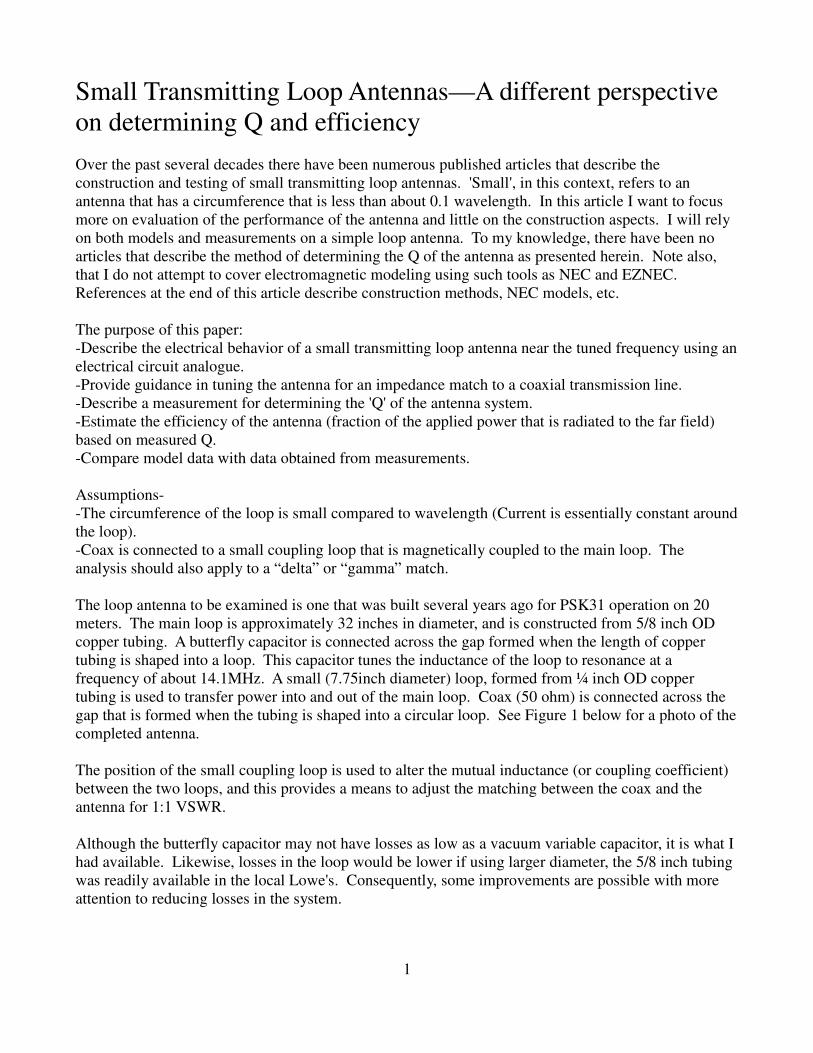
The loop antenna to be examined is one that was built several years ago for PSK31 operation on 20

meters. The main loop is approximately 32 inches in diameter, and is constructed from 5/8 inch OD

copper tubing. A butterfly capacitor is connected across the gap formed when the length of copper

tubing is shaped into a loop. This capacitor tunes the inductance of the loop to resonance at a

frequency of about 14.1MHz. A small (7.75inch diameter) loop, formed from ¼ inch OD copper

tubing is used to transfer power into and out of the main loop. Coax (50 ohm) is connected across the

gap that is formed when the tubing is shaped into a circular loop. See Figure 1 below for a photo of the

completed antenna.

The position of the small coupling loop is used to alter the mutual inductance (or coupling coefficient)

between the two loops, and this provides a means to adjust the matching between the coax and the

antenna for 1:1 VSWR.

Although the butterfly capacitor may not have losses as low as a vacuum variable capacitor, it is what I

had available. Likewise, losses in the loop would be lower if using larger diameter, the 5/8 inch tubing

was readily available in the local Lowe's. Consequently, some improvements are possible with more

attention to reducing losses in the system.

1

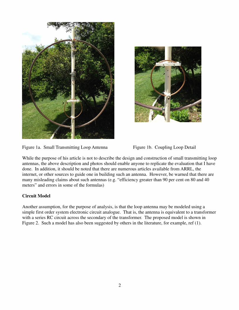
Figure 1a. Small Transmitting Loop Antenna Figure 1b. Coupling Loop Detail

While the purpose of his article is not to describe the design and construction of small transmitting loop

antennas, the above description and photos should enable anyone to replicate the evaluation that I have

done. In addition, it should be noted that there are numerous articles available from ARRL, the

internet, or other sources to guide one in building such an antenna. However, be warned that there are

many misleading claims about such antennas (e.g. “efficiency greater than 90 per cent on 80 and 40

meters” and errors in some of the formulas)

Circuit Model

Another assumption, for the purpose of analysis, is that the loop antenna may be modeled using a

simple first order system electronic circuit analogue. That is, the antenna is equivalent to a transformer

with a series RC circuit across the secondary of the transformer. The proposed model is shown in

Figure 2. Such a model has also been suggested by others in the literature, for example, ref (1).

2

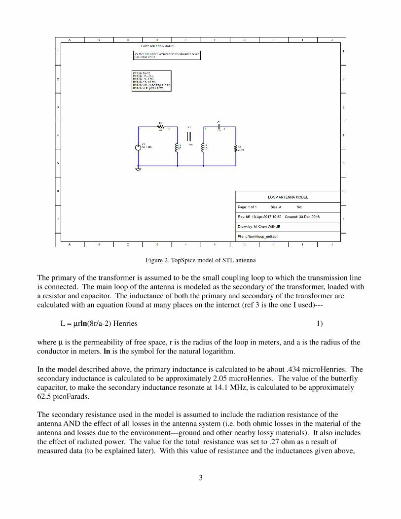
Figure 2. TopSpice model of STL antenna

The primary of the transformer is assumed to be the small coupling loop to which the transmission line

is connected. The main loop of the antenna is modeled as the secondary of the transformer, loaded with

a resistor and capacitor. The inductance of both the primary and secondary of the transformer are

calculated with an equation found at many places on the internet (ref 3 is the one I used)---

L = µrln(8r/a-2) Henries 1)

where µ is the permeability of free space, r is the radius of the loop in meters, and a is the radius of the

conductor in meters. ln is the symbol for the natural logarithm.

In the model described above, the primary inductance is calculated to be about .434 microHenries. The

secondary inductance is calculated to be approximately 2.05 microHenries. The value of the butterfly

capacitor, to make the secondary inductance resonate at 14.1 MHz, is calculated to be approximately

62.5 picoFarads.

The secondary resistance used in the model is assumed to include the radiation resistance of the

antenna AND the effect of all losses in the antenna system (i.e. both ohmic losses in the material of the

antenna and losses due to the environment—ground and other nearby lossy materials). It also includes

the effect of radiated power. The value for the total resistance was set to .27 ohm as a result of

measured data (to be explained later). With this value of resistance and the inductances given above,

3

electrical simulations and measured results are in close agreement.

To analyze the circuit in Figure 2, I use the free (demo) Version 8 of TopSpice (www.penzar.com).

This program was chosen because of previous experience with TopSpice and its ability to generate

SmithCharts. Although the demo version is limited in the number of components and nodes, it suffices

for the simple model we want to analyze.

To gain further insight into the the model, I also derived the equations that apply to the circuit. Using

simple current loop equations, the input impedance to the antenna (at the point the coax is connected to

the coupling loop) is found to be given by:

Zin(ω) = jωLp +(ωM)2/Zs(ω), where Zs(ω) is the series impedance of the secondary. 2)

Zs(ω) = Rs +jωLs +1/jωCs 3)

In this equation, Lp is the inductance of the coupling loop, Ls is the inductance of the main loop, Cs is

the capacitance value of the butterfly tuning capacitance (including any “stray” capacitance) and Rs is

the resistance that accounts for all power “loss” in the antenna system (including that which is

radiated). In order to more easily understand the behavior of the antenna near resonance, I have used a

change of variables in the equation for the input impedance. I have also employed the commonly used

expression for the 'Q' of the tuned circuit.

Additionally, the mutual inductance between the primary and secondary will be represented by the

coupling coefficient k using the formula

M2 = k2LpLs 4)

The resonant frequency of a series tuned circuit is given by f0=1/2π√LsCs

The Q factor is Q=ω0Ls/Rs where ω0=2πf0

Since we are interested in the behavior of the antenna near its resonant frequency, we make the

substitution f=f0*(1+δ) , where |δ| is much smaller than unity.

Without going into the detailed manipulation of the equation for the input impedance, it may be shown

that

Zin(δ) = jω0Lp(1+δ) + ((ω02M2(1+δ)2)/Zs(δ) 5)

Zs(δ) =Rs + jω0Ls(1+δ) + 1/(jω0Cs(1+δ)) 6)

Using the common definition of Q, shown above, the equation for the input impedance may be

simplified to

Zin(δ) = jω0Lp(1+δ) + (1+2δ)k2Q(1+j2δQ) 7)

Note: In the above expression, we have made the substitution (1+δ)2 = 1+2δ and 1/(1+δ) = 1-δ. As

long as |δ| is <<1, this should introduce negligible error. As you will see later, the calculated

4

impedance matches measured data very closely. These approximations imply that we have a high Q

system.

This equation will be used to examine the Real and Imaginary parts of the input impedance as a

function of the deviation of the frequency from the self-resonant frequency of the loop. The actual

frequency deviation is δ times the resonant frequency f0.

The real part of Zin(δ) is given by

Re(Zin(δ)) = ω0Lp(1+2δ)k2Q/(1+4δ2Q2) 8)

The imaginary part of Zin(δ) is given by

Im(Zin(δ)) = ω0Lp((1+δ) – (1+2δ)2δk2Q2/(1+4δ2Q2)) 9)

At resonance, we also want to satisfy two conditions--

Re(Zin(δ)) = Z0 and 10)

Im(Zin(δ)) = 0 11)

Z0 is the characteristic impedance of the coax transmission line, nominally 50 ohms.

From the condition on the real part we have

ω0Lp(1+2δ)k2Q/(1+4δ2Q2) = Z0 12)

or, (1+2δ)k2Q/(1+4δ2Q2) = Z0/ ω0Lp 13)

If we now insert expression 13) into 9) for the imaginary part of Zin(δ) we obtain the following-

Im(Zin(δ)) = ω0Lp((1+δ) – 2δQZ0/ ω0Lp) 14)

Setting this expression to 0, as required for resonance, we have

δres = 1/(2QZ0/ ω0Lp – 1) 15)

Therefore, when the frequency f is f0(1+ δres), the real part of the impedance will be Z0 and the

imaginary part will be 0.

We can now return to the expression 8) for the real part of the impedance to determine what coupling

coefficient is needed to achieve Z0 ohms for the real part. After some manipulation, we obtain-

k2 = Z0(1+4 δres 2Q2)/ω0Lp(1+2δres)Q 16)

In practice, we do not have to solve this equation for the coupling coefficient as we usually adjust the

coupling to achieve the desired resonance condition using either an impedance analyzer, or an SWR

bridge. However, it may be enlightening to make the calculation once we have an estimate of the Q.

5

Determination of the Q of the antenna

The Q of the antenna is of interest for two main reasons. First, the usable bandwidth (without the need

for retuning) is determined by the Q and, second, the efficiency of the antenna is dependent on Q.

It has been proposed (3-5) that the Q of an RLC circuit can be determined from VSWR measurement. I

have confirmed mathematically, using the circuit model, that VSWR measurements can, indeed, be

used to estimate the Q. However, for the method to work, the VSWR must be very close to 1:1 at the

operating frequency. When this condition is met, if one determines frequencies on either side of

resonance, where the VSWR reaches a specific level, the difference in frequencies at the specified

VSWR level, divided into the frequency at 1:1 VSWR provides a number that is proportional to the Q

of the antenna. For example, when the target VSWR is chosen to be 3:1, f0/(f1_3-f2_3) is Q/1.154. When

the target VSWR is 2.618, f0/(f1_2.618-f2_2.618) is numerically equal to Q. At a target VSWR of 2:1, f0/(f1_2-

f2_2) = .707Q. These expressions agree with ones published in reference 5. In the expressions above,

f1-xx and f2-xx are the two frequencies on either side of resonance where the VSWR reaches the value xx.

Since using the VSWR method to determine Q requires a good match (VSWR very close to 1:1), I

decided to look at an alternative method. Using plots of the real and imaginary part of Zin obtained

from the Spice model, Figure 3, it is obvious that changes in the coupling coefficient between the small

and large loops have very small effect on the frequencies at which the imaginary part of Z has its

maximum and minimum values (close to the resonant frequency f0). This led me to further analyze the

expression for the imaginary part of Zin, particularly, in the vicinity of f0.

Recall equation 9) for the imaginary part of Zin(δ)

Im(Zin(δ)) = ω0Lp((1+δ) – (1+2δ)2δk2Q2/(1+4δ2Q2)) 17)

Since δ is very small, we can approximate Im(Zin(δ)) with ω0Lp(1-2δk2Q2/(1+4δ2Q2)). We then

differentiate this expression with respect to δ and set the derivative to zero to locate the maximum and

minimum values as a function of δ. This yields the result that when δ = +/- 1/2Q, the imaginary part

of the input impedance will have either a maximum or minimum value.

Pursuing this further, we will now focus on the Spice model results.

The following figure 3 is an output from the TopSpice program showing the behavior of the real and

imaginary parts of the input impedance close to the resonant frequency f0.

6

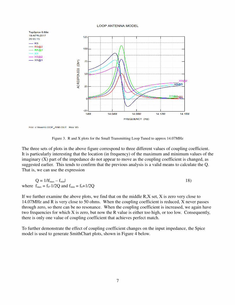
Figure 3. R and X plots for the Small Transmitting Loop Tuned to approx 14.07MHz

The three sets of plots in the above figure correspond to three different values of coupling coefficient.

It is particularly interesting that the location (in frequency) of the maximum and minimum values of the

imaginary (X) part of the impedance do not appear to move as the coupling coefficient is changed, as

suggested earlier. This tends to confirm that the previous analysis is a valid means to calculate the Q.

That is, we can use the expression

Q = 1/|fmax – fmin| 18)

where fmax = f0-1/2Q and fmin = f0+1/2Q

If we further examine the above plots, we find that on the middle R,X set, X is zero very close to

14.07MHz and R is very close to 50 ohms. When the coupling coefficient is reduced, X never passes

through zero, so there can be no resonance. When the coupling coefficient is increased, we again have

two frequencies for which X is zero, but now the R value is either too high, or too low. Consequently,

there is only one value of coupling coefficient that achieves perfect match.

To further demonstrate the effect of coupling coefficient changes on the input impedance, the Spice

model is used to generate SmithChart plots, shown in Figure 4 below.

7

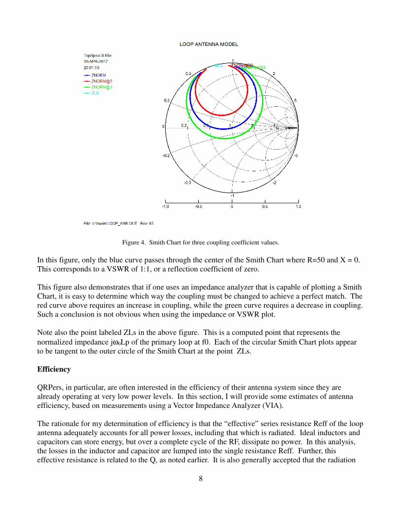
Figure 4. Smith Chart for three coupling coefficient values.

In this figure, only the blue curve passes through the center of the Smith Chart where R=50 and X = 0.

This corresponds to a VSWR of 1:1, or a reflection coefficient of zero.

This figure also demonstrates that if one uses an impedance analyzer that is capable of plotting a Smith

Chart, it is easy to determine which way the coupling must be changed to achieve a perfect match. The

red curve above requires an increase in coupling, while the green curve requires a decrease in coupling.

Such a conclusion is not obvious when using the impedance or VSWR plot.

Note also the point labeled ZLs in the above figure. This is a computed point that represents the

normalized impedance jω0Lp of the primary loop at f0. Each of the circular Smith Chart plots appear

to be tangent to the outer circle of the Smith Chart at the point ZLs.

Efficiency

QRPers, in particular, are often interested in the efficiency of their antenna system since they are

already operating at very low power levels. In this section, I will provide some estimates of antenna

efficiency, based on measurements using a Vector Impedance Analyzer (VIA).

The rationale for my determination of efficiency is that the “effective” series resistance Reff of the loop

antenna adequately accounts for all power losses, including that which is radiated. Ideal inductors and

capacitors can store energy, but over a complete cycle of the RF, dissipate no power. In this analysis,

the losses in the inductor and capacitor are lumped into the single resistance Reff. Further, this

effective resistance is related to the Q, as noted earlier. It is also generally accepted that the radiation

8

resistance, which is part of the effective resistance, represents power which is radiated by the structure

and is therefore lost.

The following formula, found in the literature (2), is used to calculate the radiation resistance Rrad,

based on the loop structure.

Rrad = 197Cλ4, 19)

where Cλ is the circumference of the loop in wavelengths.

Allow Irf to represent the RF current that flows in the loop. Therefore, the power that is dissipated in

the loop is given by

Ptotal = Irf2*Reff 20)

and the power radiated is represented by

Prad = Irf2*Rrad 21)

The fraction of the total power that is radiated (or efficiency) is therefore given by the ratio of Rrad to

Reff

efficiency=100 x Prad/Ptotal = 100 x Rrad/Reff 22)

However, since the Q of the antenna is given by

Q = ωLs/Reff (remember Reff is the same as the Spice Model Rs) 23)

we can also express efficiency as

efficiency = 100 x RradQ/ωLs 24)

This tells us that the only options we have for increasing efficiency is to increase Rrad or Q. Rrad may

be increased by making the loop larger. Q may be increased by using lower loss materials.

Measurements on a “Real” Loop Antenna

Next we discuss measurements made using a Vector Impedance Analyzer (VIA) offered by the Austin

Texas QRP group. For information on the VIA, see http://www.qsl.net/k5bcq/Kits/Kits.html

The VIA is first calibrated using a short piece of 50 ohm coax between the VIA and the open, short, and

calibration resistor. This makes the measurement point at the end of the coax, away from the VIA.

The antenna is initially set with the plane of the small loop parallel to the plane of the main loop. The

small coupling loop is positioned so that no point on its circumference is closer to the main loop than

about 1 inch. Also, as shown in Figure 1, the coupling loop is mounted diametrically opposite from the

9

tuning capacitor.

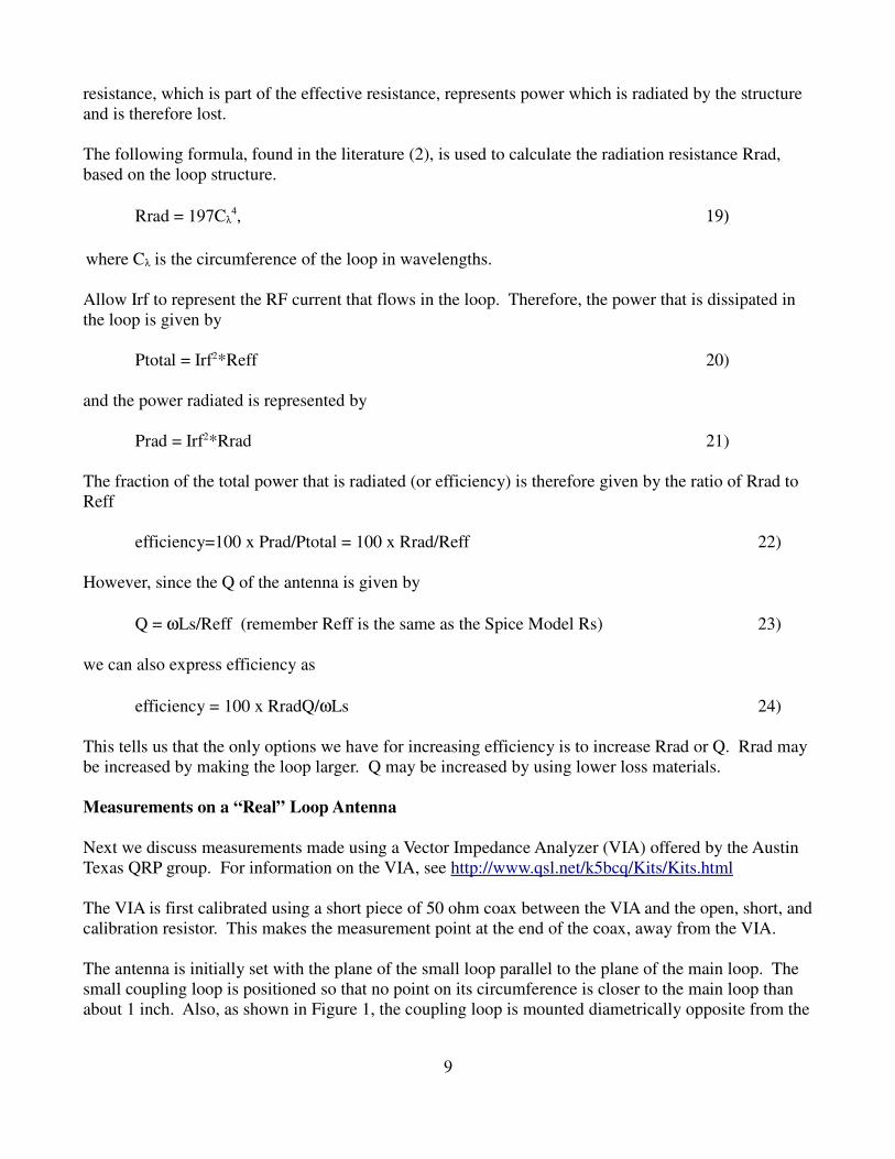
A VSWR scan is then run over a wide frequency range to determine the approximate tuned frequency.

See Figure 5. The tuning capacitor is adjusted, as needed, to set the operating frequency of the antenna

as close to 14.1MHz as possible. Having done this, the scan range of the VIA is reduced to a few

hundred kHz and recalibrated (not needed with the latest firmware in the VIA) –Figure 6. We then

scan the new range, using the Smith Chart plot option on the VIA-- Figure 7. Note the similarity to

Figure 4, above. This plot lets us know whether the coupling between the small and large loops is too

little, or too much. If the plot does not encircle the center of the chart, then the coupling is too little. If

the plot does encircle the chart center, then the coupling needs to be reduced.

Figure 5. Broad VSWR Scan (10 to 20MHz)

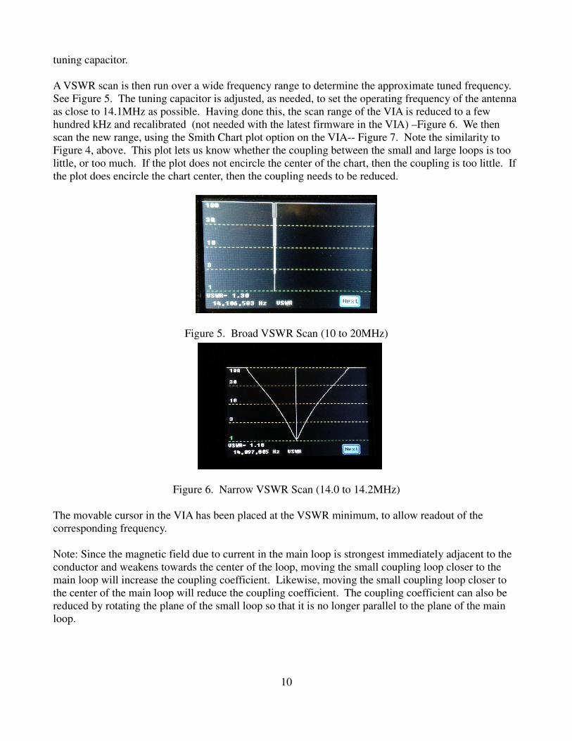
Figure 6. Narrow VSWR Scan (14.0 to 14.2MHz)

The movable cursor in the VIA has been placed at the VSWR minimum, to allow readout of the

corresponding frequency.

Note: Since the magnetic field due to current in the main loop is strongest immediately adjacent to the

conductor and weakens towards the center of the loop, moving the small coupling loop closer to the

main loop will increase the coupling coefficient. Likewise, moving the small coupling loop closer to

the center of the main loop will reduce the coupling coefficient. The coupling coefficient can also be

reduced by rotating the plane of the small loop so that it is no longer parallel to the plane of the main

loop.

10

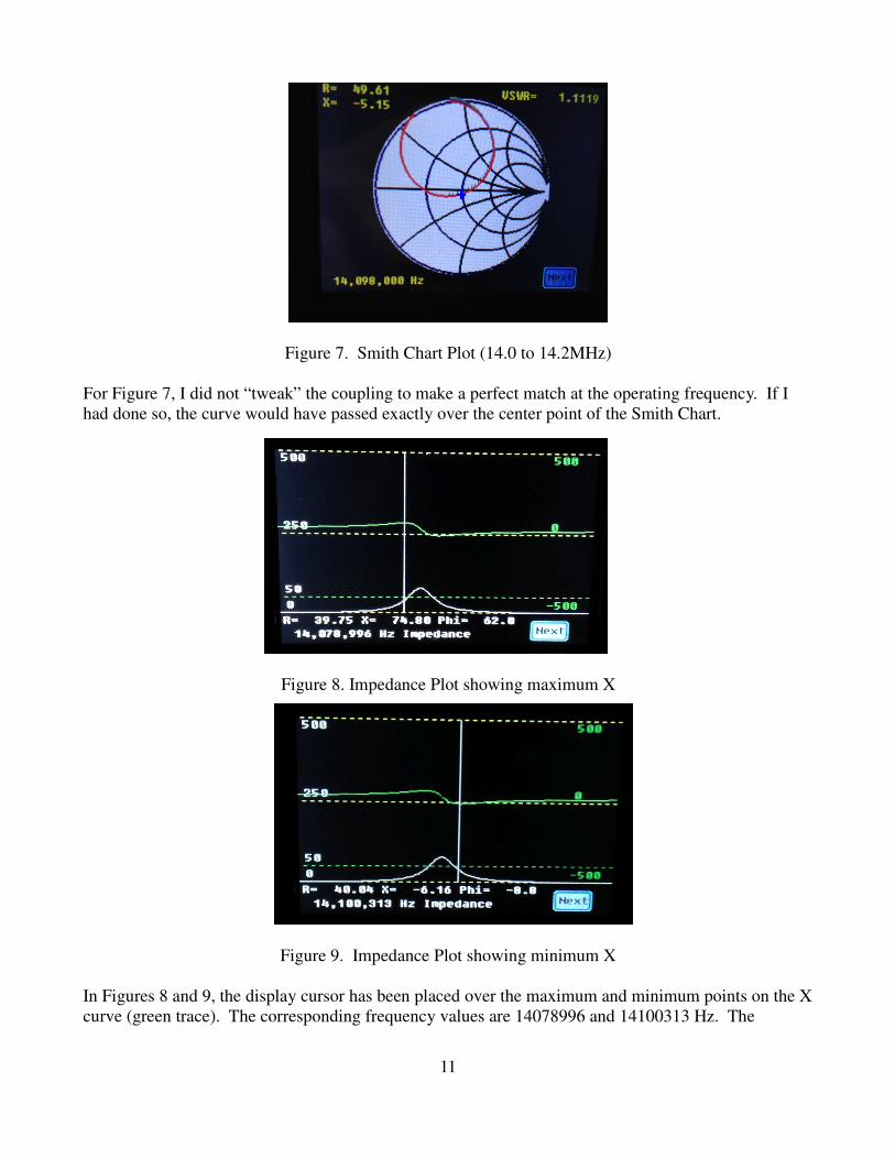
Figure 7. Smith Chart Plot (14.0 to 14.2MHz)

For Figure 7, I did not “tweak” the coupling to make a perfect match at the operating frequency. If I

had done so, the curve would have passed exactly over the center point of the Smith Chart.

Figure 8. Impedance Plot showing maximum X

Figure 9. Impedance Plot showing minimum X

In Figures 8 and 9, the display cursor has been placed over the maximum and minimum points on the X

curve (green trace). The corresponding frequency values are 14078996 and 14100313 Hz. The

11

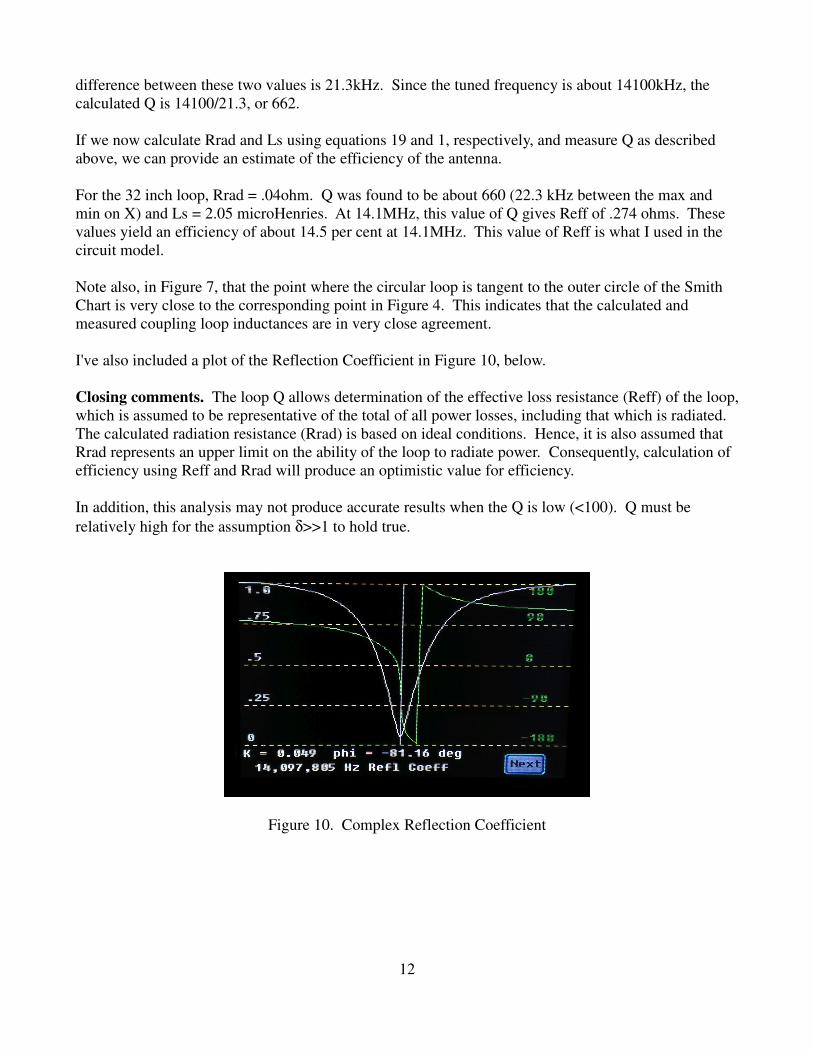
difference between these two values is 21.3kHz. Since the tuned frequency is about 14100kHz, the

calculated Q is 14100/21.3, or 662.

If we now calculate Rrad and Ls using equations 19 and 1, respectively, and measure Q as described

above, we can provide an estimate of the efficiency of the antenna.

For the 32 inch loop, Rrad = .04ohm. Q was found to be about 660 (22.3 kHz between the max and

min on X) and Ls = 2.05 microHenries. At 14.1MHz, this value of Q gives Reff of .274 ohms. These

values yield an efficiency of about 14.5 per cent at 14.1MHz. This value of Reff is what I used in the

circuit model.

Note also, in Figure 7, that the point where the circular loop is tangent to the outer circle of the Smith

Chart is very close to the corresponding point in Figure 4. This indicates that the calculated and

measured coupling loop inductances are in very close agreement.

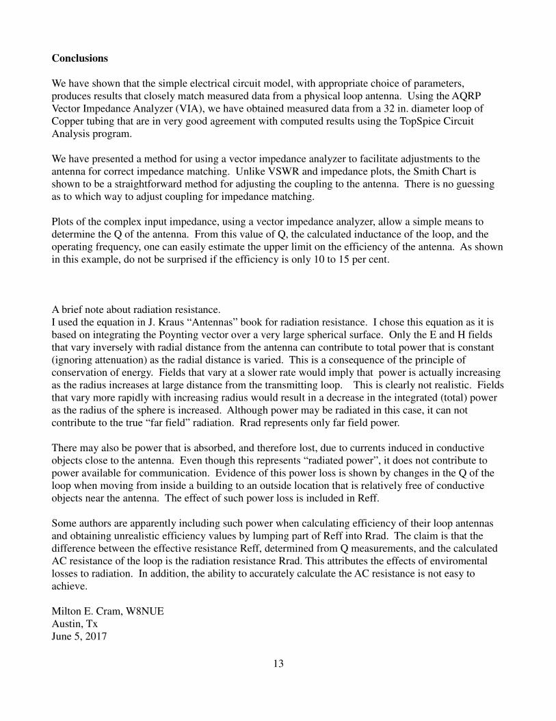
I've also included a plot of the Reflection Coefficient in Figure 10, below.

Closing comments. The loop Q allows determination of the effective loss resistance (Reff) of the loop,

which is assumed to be representative of the total of all power losses, including that which is radiated.

The calculated radiation resistance (Rrad) is based on ideal conditions. Hence, it is also assumed that

Rrad represents an upper limit on the ability of the loop to radiate power. Consequently, calculation of

efficiency using Reff and Rrad will produce an optimistic value for efficiency.

In addition, this analysis may not produce accurate results when the Q is low (<100). Q must be

relatively high for the assumption δ>>1 to hold true.

Figure 10. Complex Reflection Coefficient

12

Conclusions

We have shown that the simple electrical circuit model, with appropriate choice of parameters,

produces results that closely match measured data from a physical loop antenna. Using the AQRP

Vector Impedance Analyzer (VIA), we have obtained measured data from a 32 in. diameter loop of

Copper tubing that are in very good agreement with computed results using the TopSpice Circuit

Analysis program.

We have presented a method for using a vector impedance analyzer to facilitate adjustments to the

antenna for correct impedance matching. Unlike VSWR and impedance plots, the Smith Chart is

shown to be a straightforward method for adjusting the coupling to the antenna. There is no guessing

as to which way to adjust coupling for impedance matching.

Plots of the complex input impedance, using a vector impedance analyzer, allow a simple means to

determine the Q of the antenna. From this value of Q, the calculated inductance of the loop, and the

operating frequency, one can easily estimate the upper limit on the efficiency of the antenna. As shown

in this example, do not be surprised if the efficiency is only 10 to 15 per cent.

A brief note about radiation resistance.

I used the equation in J. Kraus “Antennas” book for radiation resistance. I chose this equation as it is

based on integrating the Poynting vector over a very large spherical surface. Only the E and H fields

that vary inversely with radial distance from the antenna can contribute to total power that is constant

(ignoring attenuation) as the radial distance is varied. This is a consequence of the principle of

conservation of energy. Fields that vary at a slower rate would imply that power is actually increasing

as the radius increases at large distance from the transmitting loop. This is clearly not realistic. Fields

that vary more rapidly with increasing radius would result in a decrease in the integrated (total) power

as the radius of the sphere is increased. Although power may be radiated in this case, it can not

contribute to the true “far field” radiation. Rrad represents only far field power.

There may also be power that is absorbed, and therefore lost, due to currents induced in conductive

objects close to the antenna. Even though this represents “radiated power”, it does not contribute to

power available for communication. Evidence of this power loss is shown by changes in the Q of the

loop when moving from inside a building to an outside location that is relatively free of conductive

objects near the antenna. The effect of such power loss is included in Reff.

Some authors are apparently including such power when calculating efficiency of their loop antennas

and obtaining unrealistic efficiency values by lumping part of Reff into Rrad. The claim is that the

difference between the effective resistance Reff, determined from Q measurements, and the calculated

AC resistance of the loop is the radiation resistance Rrad. This attributes the effects of enviromental

losses to radiation. In addition, the ability to accurately calculate the AC resistance is not easy to

achieve.

Milton E. Cram, W8NUE

Austin, Tx

June 5, 2017

13

References

1) Alan Boswell, Andrew J. Tyler, and Adam White, “Performance of a Small Loop Antenna in the

3-10 MHz Band” Downloaded from IEEE Explore March 24, 2010

2) J. Kraus, “Antennas”, McGraw Hill, 1950

3) https://technick.net/tools/inductance-calculator/circular-loop

4) A. D. Yaghjian and S. R. Best, “Impedance, Bandwidth and Q

of Antennas,” IEEE Intemational Symposium on Antennas and

Propagation Digest, 1, Columbus, Ohio, June 2003, pp. 501-504.

5) http://www.aa5tb.com/loop.html

6) http://gridtoys.com/glen/loop/loop3.html

7) http://owenduffy.net/blog/?p=4888

8) http://www.qsl.net/kp4md/magloophf.htm

9) https://www.nonstopsystems.com/radio/frank_radio_antenna_magloop.htm

10) A. D. Yaghian and S. R. Best, “Impedance, Bandwidth, and Q of Antennas”, IEEE International

Symposium on Antennas and Propagation, Digest 1, Columbus, Ohio June 2003, pp 501-504

11) John S. Belrose, “Performance of Electrically Small Tuned Transmitting Loop Antennas”

Radcom, Radio Society of Great Britain, London, UK, June/July 2004

12) Mike Underhill, “Small Loop Antenna Efficiency” Presented in Kempton UK, May 2006

14