Smith's Rule In Stochastic Scheduling - iasi.cnr.it · IntroRelated WorkPreliminariesThe ResultEnd Smith’s Rule In Stochastic Scheduling Caroline Jagtenberg Uwe Schwiegelshohn Marc

Intro Related Work Preliminaries The Result End

Smith’s Rule In Stochastic Scheduling

Caroline Jagtenberg Uwe Schwiegelshohn Marc UetzUtrecht University Dortmund University University of Twente

Aussois 2011

Marc Uetz Smith’s Rule in Stochastic Scheduling


The (classic) setting

Problem

n jobs, nonpreemptive, processing times pj and weights wj

m identical, parallel machines

Cj = completion time of job j

goal: minimize total weighted completion time,∑

wjCj

P| |∑

wjCj (thanks JKL)

Complexity

The problem is (strongly) NP-hard [Bruno et al. 1974]

PTAS exists [Skutella and Woeginger, 2000]



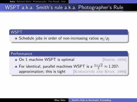
WSPT a.k.a. Smith’s rule a.k.a. Photographer’s Rule

WSPT

Schedule jobs in order of non-increasing ratios wj/pj

Performance

On 1 machine WSPT is optimal [Smith, 1956]

For identical, parallel machines WSPT is a 1+√

22 ≈ 1.207-

approximation; this is tight [Kawaguchi and Kyan, 1986]



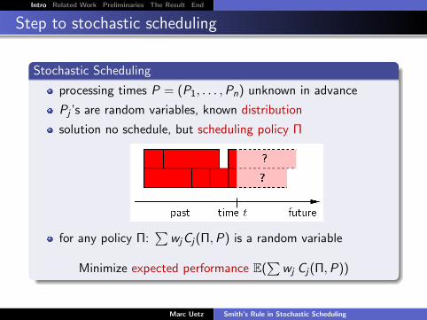
Step to stochastic scheduling

Stochastic Scheduling

processing times P = (P1, . . . ,Pn) unknown in advance

Pj ’s are random variables, known distribution

solution no schedule, but scheduling policy Π

for any policy Π:∑

wjCj(Π,P) is a random variable

Minimize expected performance E(∑

wj Cj(Π,P))



Complexity of (general) stochastic scheduling

In general, optimal policies are NP-hard to find

Calculating the objective value of a given policy can be # Pcomplete [Hagstrom 1988]

Optimal policy may require deliberate idleness [U. 2003]

Question

Does it become (significantly) easier if we restrict e.g. to onlyexponentially distributed processing times, i.e., Pj ∼ exp(λj)?

i.e., Pj ’s are memory-less, P[Pj > x + t | Pj > t] = P[Pj > x ]

Open Problem

1 Does there exist an optimal policy without deliberate idleness?



Intuition

Quote”Scheduling: Theory, Algorithms, and Systems” [Pinedo, 2002]

Example: P||Cmax is NP-hard for deterministic scheduling, but forPj ∼ exp(λj), LEPT is optimal [Weiss and Pinedo, 1980]



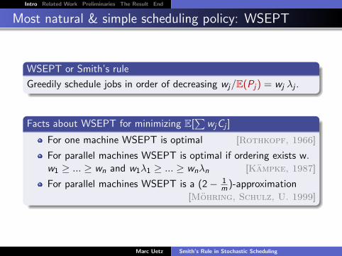
Most natural & simple scheduling policy: WSEPT

WSEPT or Smith’s rule

Greedily schedule jobs in order of decreasing wj/E(Pj) = wj λj .

Facts about WSEPT for minimizing E[∑

wjCj ]

For one machine WSEPT is optimal [Rothkopf, 1966]

For parallel machines WSEPT is optimal if ordering exists w.w1 ≥ ... ≥ wn and w1λ1 ≥ ... ≥ wnλn [Kampke, 1987]

For parallel machines WSEPT is a (2− 1m )-approximation

[Mohring, Schulz, U. 1999]



Our (Counterintuitive?) Result

Theorem

Performance of WSEPT is not better than 1.243 OPT.That is, ∃ instances where in expectation

E[∑

wjCWSEPTj ] > 1.243 E[

∑wjC

OPTj ]

Counterintuition: This is even worse than WSPT in deterministicscheduling, which is at most 1.207 OPT.

Proof

Follows from analysis and adaptation of the instance given byKawaguchi and Kyan.



Kawaguchi & Kyan (deterministic) example

x ·m big jobs with pj = wj = p, n ·m small jobs with pj = wj = 1n

Left schedule:∑

wjCj = (p2xm ) + ( 12

11−x m ) + o(1)

Right schedule:∑

wjCj = ((1 + p)pxm ) + ( 12m ) + o(1)

p = 1 +√

2 and x = 12+√

2gives a maximal ratio of 1+

√2

2 ≈ 1.207



Stochastic version of Kawaguchi & Kyan example

x ·m i.i.d. big jobs each with Pj ∼ exp(λ), and

wj := E[Pj ] =1

λ:= p

n ·m i.i.d. small jobs each with Pj ∼ exp(n), and

wj := E[Pj ] =1

n



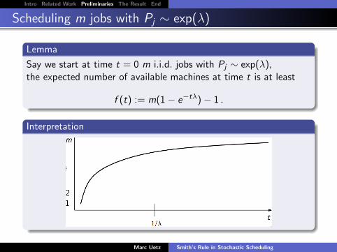
Scheduling m jobs with Pj ∼ exp(λ)

Lemma

Say we start at time t = 0 m i.i.d. jobs with Pj ∼ exp(λ),the expected number of available machines at time t is at least

f (t) := m(1− e−tλ)− 1 .

Interpretation



Behaviour of parallel jobs with Pj ∼ exp(λ)

When scheduling in parallel m jobs with i.i.d. processing timesPj ∼ exp(λ), the first completion is expected at time 1/(mλ).As Pj ’s are memory less, E[Pj − t | Pj > t] = E[Pj ] = 1/λ,the second completion is expected time 1/((m − 1)λ) later.

etc., so j th completion is expected at time tj =

j∑i=1

1

(m − i + 1)λ

Using H(m) =m∑

i=1

1

i≥ ln(m) + 0.58, find that tj ≤ 1

λ ln( mm−j ),

so # free machines at t: ≥ bm(1− e−tλ)c ≥ m(1− e−tλ)− 1



Stochastic version of (worst case) WSPT schedule

Remember Kawaguchi and Kyan’s (worst case) schedule

Machines finish processing short jobs “more or less” at t = 1E[difference] ≤ 1

n

∑m−1i=1

1i ≈ 0 (as we have n > m)

Each long job completes in expectation at time ≈ (1 + 1λ)

Hence, E[∑

wjCj ] ≈ to the deterministic case.



Stochastic version of (optimal) WSPT schedule

The expected optimal schedule of the stochastic variant:Contribution of long jobs is the same as in the deterministic case.What about the small jobs?

Compute time T such that∫ T0 f (t)dt ≥ total expected processing

volume of small jobs. How? Numerically, T = 1.2933 suffices.



We can now approximate location of small jobs.

But how much do they contribute to the objective value

E[∑

wjCj ] ?



Contribution of Small Jobs

Lemma

Consider nT jobs with i.i.d. processing times Pj ∼ exp(n) andweights wj = 1/n, scheduled on a single machine. Then for allε > 0 there exists n large enough so that

E[∑

j wjCj ] ≤∫ T

0t dt + ε .

Proof.

E[∑

j wjCj ] = 1n nT 1/n+T

2 = 12T 2 + 1

2nT =∫ T0 t dt + 1

2nT



Contribution of Small Jobs

Generalization

We can generalize this lemma for parallel machines.

Let m(t) be the number of machines available at time t, then

E[∑

j wjCj ] ≤∫ T

0m(t) t dt + ε



Comparing the objective values E[∑

wjCj ]

Ingredients

1 long jobs’ contribution same as in deterministic case

2 machines w. small jobs finish at ≈ equal times (“sand”)

3

for OPT

{# available machines ≥ f (t) = m(1− e−tλ)− 1

small jobs contribute E[∑

j wjCj ] ≤∫ T0 f (t) t dt

Putting all that together, we get

WSEPT is an α-approximation,

with α ≥ E(P

j wjCj [B])

E(P

j wjCj [A])

≥ 1.229 (n→∞,m→∞)



The result

Optimizing over # and length E[Pj ] of the long jobs

The result above was for

12+√

2m ≈ 0.29 m long jobs with E[Pj ] = 1 +

√2 ≈ 2.4

Taking for example:

0.43 m long jobs with E[Pj ] ≈ 1.8

yields α > 1.243

Theorem

For jobs with exponentially distributed processing times,WSEPT is no better than a 1.243 - approximation.



Conclusions

What we’ve found

With Pj ∼ exp(λj), WSEPT can be factor > 1.243 away fromoptimal policy (in expectation); worse than tight bound fordeterministic scheduling, ≈ 1.207 [→ WAOA 2010 proceedings]

Open Problems

2 Instance(s) where WSEPT performs even worse?

3 I’d rather go and improve the upper bound (2− 1/m) !

4 Stochastic scheduling for Pj ∼ exp(λj), hard at all?

5 And the complexity of computing E[∑

j wjCWSEPTj ]?



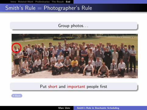
Smith’s Rule = Photographer’s Rule

Group photos. . .

Put short and important people first

Back


Documents

Smith's Rule In Stochastic Scheduling - iasi.cnr.it · IntroRelated WorkPreliminariesThe ResultEnd Smith’s Rule In Stochastic Scheduling Caroline Jagtenberg Uwe Schwiegelshohn Marc