NEA/NSC-DOC (96)29 AUGUST 1996

SMORN-VII

REPORTNEURAL NETWORK BENCHMARK

ANALYSIS RESULTS & FOLLOW-UP’96

Özer CIFTCIOGLUIstanbul Technical University, ITU

and

Erdinç TÜRKCANNetherlands Energy Research Foundation, ECN

VOLUME I(Revised, August 1998)

SMORN VIIA symposium on Nuclear Reactor

Surveillance and Diagnostics13-19 June, 1995, Avignon (FRANCE)

1

NEURAL NETWORKBENCHMARK FOR

SMORN-VIIANALYSIS RESULTS & FOLLOW-UP’96

Özer CIFTCIOGLUIstanbul Technical University, ITU

Electrical & Electronics Engineering Faculty, Istanbul, Turkey

and

Erdinç TÜRKCANNetherlands Energy Research Foundation, ECN

P.O. Box 1, 1755 ZG Petten, The Netherlands

SMORN VIIA symposium on Nuclear Reactor

Surveillance and Diagnostics13-19 June, 1995, Avignon (FRANCE)

2

This work is accomplished under the auspices of OECD with an exclusive agreementbetween OECD and the first author affiliated with ITU.Contract ref.: PERS/U3/96/509/AN/AMH.

NOTICE

1996All rights are at the discretion of OECD

The document is available at the web site:http://www.nea.fr/html/science/rsd/

All correspondences should be addressed to:Prof. Dr. Özer Ciftcioglu

Delft University of TechnologyInformatica, BK 5eBerlage weg 12629 CR DelftThe Netherlands

Tel : +31-15 2784485Fax : +31-15 2784127E-Mail: ciftciog@bk.tudelft.nl

3

CONTENTS

page

Foreword

Summary 1

1. Introduction 2

2. Neural Networks2.1. Network structures 62.2. Learning algorithms 9 2.2.1. Supervised Learning algorithms 10 2.2.2. Unsupervised Learning Algorithms 212.3. Sensitivity 23

3. Analysis of the Benchmark Results Reported 24

4. Further Studies with the Benchmark Data4.1. Advanced learning algorithms 304.2. Sensitivity analysis 34

5. NN Benchmark Follow-up’96 35

6. Conclusions 38

REFERENCES 119

APPENDIX 120

A-1 :Extended Summary

A-2 :Questionnaire of the Benchmark Tasks

A-3 :Reported results by participants

4

FOREWORD

NEURAL NETWORK BENCHMARK FOR SMORN-VIIANALYSIS RESULTS: FOLLOW-UP’96

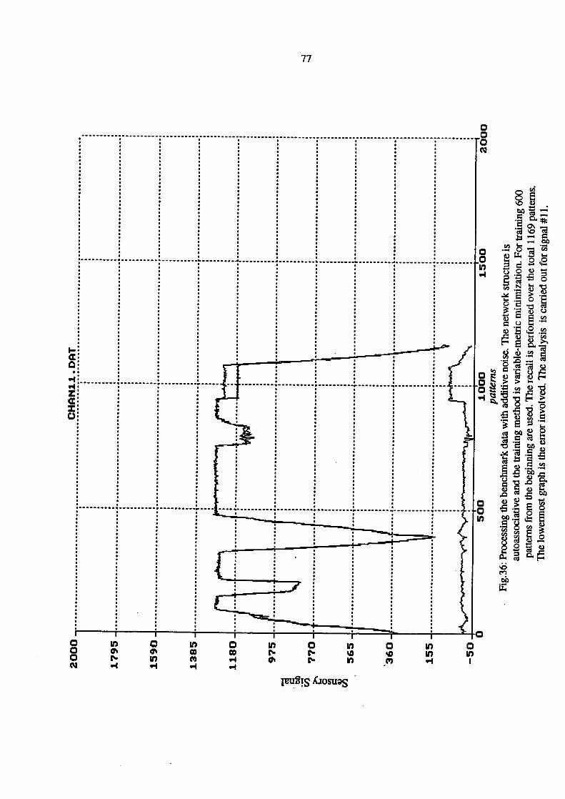
This work is a comprehensive final analysis report of the neural network benchmark(Benchmark-95) presented at SMORN-VII. The report contains the formal analysis of boththe benchmark-data for the prescribed formal tasks and additionally some optional items placedin the benchmark exercise for optional further analyses. Altogether, the work carried out is acomprehensive study of the benchmark exercise using different approaches in neural network(NN) training and performing respective evaluations of the results. Finally, the benchmarkanalysis results reported by each participant are addressed, evaluated and documented in thereport.

The work as a whole establishes some guidelines for neural network implementation especiallyfor the applications in process system monitoring for safety and cost effective operation. Insuch applications the source of information is measurement data obtained from the process orplant sensors with random measurement errors. Therefore, the benchmark data are so preparedthat they comprise the measurements obtained from an operating actual nuclear power plant tobenefit the participants maximally as a return for their appreciable participation efforts.

The generalization capability is an important concept in the terminology of neural networks. Inthis respect, in the benchmark data distributed, rinsing and stretch-out operations areimportant modes for the evaluation of the neural network performance. Along this line, anotherimportant related issue is the concept of neural network sensitivity where the sensitivity shoulddesirably be distributed evenly among the input-output signals. In the report, these topics arehighlighted, investigated and the results are evaluated in the form of a research work beyondthe prescribed formal analyses and foreseen tasks.

Considering this rather involved scope of Benchmark-95, the present study gives someindications about the state-of-the-art-functionality of the neural network technology forinformation processing and determines some guidelines for the effective neural networkutilization especially having the industrial process monitoring, like a power plant for instance, inview.

5

SUMMARY

A neural network (NN) benchmarks designed for condition monitoring in nuclear reactors isdescribed. As the neural network is a new technology arose in the last decade, its potentiality isgetting recognized only recently and its utilization is already taking place in industrialapplications. In this respect, the utilization of neural networks in nuclear reactors is alsoincreasing for diverse applications. Among the most beneficial utilization one can refer to costeffective plant operation and plant monitoring and surveillance with enhanced safety which aredue to the features inherently laying in the neural structure. The former is related to totalproductive maintenance including plant life extension. From the reactor noise analysisviewpoint, neural networks can be used for stochastic signal processing and spectral estimationsas well as for processing operational information from gross plant signals. In the benchmark,which is shortly referred to as NN Benchmark-95, the latter, that is, information using grossplant signals from the detectors describing the operational status is considered because of bothrelatively easy processing of these signals with neural network and relatively easy evaluation ofthe results. The NN Benchmark-95 evaluation results have been globally disclosed at thesymposium SMORN-VII and an extended summary have been presented. In this report, inaddition to the comprehensive benchmark analysis results the benchmark data preparation isbriefly described and the relevant tasks to be carried out by the participants are given for thecompleteness of the work. Also the prescribed tasks executed by the benchmark organizers areillustrated for guidance referring to both, the present participants and later probableembankments on the analysis of the benchmark data by prospective newcomers. This finalreport at hand is a comprehensive evaluation of the benchmark tasks analysis results submittedfor formal participation and some elaboration on the optional tasks. Additionally, in the light ofthese considerations a follow-up of the NN Benchmark-95 is designed for prospectiveparticipants for the purpose of providing further insight into information processing by neuralnetworks for enhanced utilization of this emerging technology in the nuclear technology.

6

1. INTRODUCTION

Although the neural networks, as a new information processing methodology, have appearedonly in the last decade, the rapid growth of the research in this field is quite conspicuous. Theapplications almost in all engineering fields as well as in the soft sciences and other diverseareas resulted in a new technology known as Neural Network Technology today. The morerecent growth of interest on the subject apparently to be caused by their promise to yieldsolutions that traditional approaches do not yield. Neural network (NN) is loosely articulated inthe context of artificial intelligence, and therefore named as artificial neural networks, in theliterature. It is claimed that it resembles the brain in some respects. In this context neuralnetwork can be defined as follows. A neural network is a distributed information processorwhere structural information can be stored and can be made available for use in later reference.It resembles the brain functions because the network through a learning process acquiresknowledge and the information/knowledge stored is distributed in the form of connectionweights of the network structure as brain does through synaptic weights connecting biologicalneurons to each other.

From the viewpoint of nuclear technology, in particular for power plant operation, the use ofneural networks provides the following useful properties and capabilities.

1. Non-linearity. The non-linearity is the inherent property of the neural network as it storesknowledge. By this property, the nonlinear relationships between the plant signals can easily bemodeled.

2. Pattern recognition. The most beneficial use of pattern recognition property in plantoperation is presumably due to the input-output mapping performed by the network. Thenetwork learns from the examples by constructing an input-output mapping of the plant signals.Once this mapping is established through the learning process, responding to multi inputexcitations and observing deviations from this mapping scheme at the output of the network is apotential tool for monitoring and surveillance. Explicitly, a neural network may be designed soas to classify an input pattern as one of several predefined types of fault states of a power plantand afterwards for easy recognition of such a state in critical situations. These applications havedemonstrated high performance. A more elaborated relevant application is for accidentmanagement [1].

3. Adaptivity. By adaptivity, a neural network can operate in a non-stationary environment andit can be used for adaptive pattern classification like normal-abnormal status decision making inan operating plant. In particular, one can refer their ability to respond in real-time to thechanging system-state descriptions provided by continuous sensor input. For a nuclear powerplant where many sensors are used, the real-time response is a challenge to both humanoperators and expert systems. In this context, the integration of a neural network with an expertsystem provides neural network utilization with a substantial potentiality for fault diagnosis. Inthis case, monitoring system thus formed gains the functionality of being an operating supportsystem as the decisions made are based on the power plant knowledge base of the expertsystem.

4. Fault tolerance. In hardware form, fault tolerance of a neural network refers to theperformance of the network that it is degraded gracefully under adverse operating

7

conditions. In software form, the same refers to the performance of the network where a neuralnetwork has the ability to recognize patterns, even the information making up these patterns isnoisy or incomplete. Because of this very feature, the adaptive neural networks are highlysuited for fault diagnosis and control and risk evaluation in nuclear power plant environments.

Neural network is a generic name for a number of different constructions where artificial neuralnodes are connected among themselves. The connections are called as (synaptic) weights.Presumably, feed-forward neural networks are the most popular types among others. Manyreported works with these types of networks indicated the recognition of neural networktechnology today. Although the reported outcomes showed the desire for effective utilizationand exploitation of the potentiality of this technology, globally, there is no consensus about theexact form of forming the network structure and the training procedures. In other words, for thesame data and network type, there are many different choices for forming the network structureas well as for its training with different input parameters apart from a number of differentchoices of input data reduction and/or preparation. Therefore the comparison of differentapproaches would be very informative to get insight into understanding the nature of differencesamong the various neural networks’ performances and establish some general rules to beobserved for enhanced utilization of neural networks.

From the above described viewpoint it was decided to establish a benchmark exercise forinvestigation of potential utilization of neural networks in condition monitoring in power plantsand try to establish some basic common understanding for the application of this emergingtechnology. By means of this some standard rules of utilization or recommendations could beconcluded and everyone working actively in this field could benefit. Hence, it is anticipated thatthe exercise would reveal or shade some light on the applicability of neural network technologyin nuclear industry for monitoring.

To this end, a set of real plant data for condition monitoring exercise from the plant sensorysignals is prepared having in mind that the condition monitoring is the common feature of allmodern maintenance technologies and in this respect the data at hand would be of generalconcern. The data were distributed to the participants by OECD-NEA to carry out the tasks ofthe benchmark exercise and reporting as feedback. They are asked to report their results in aprescribed form for precise comparisons among the reported results. This would also providethe benchmark organizers with the possibility of reproducibility of reported results for thepurpose of probable detailed studies.

With reference to the scope of SMORN VII, neural networks formed a new technology that canbe closely associated with the reactor noise analysis studies and the associated technologies.Because of this newly emerging feature and concerning their actual utilization in industry,neural networks are not widely known to the community of SMORN. Therefore to disseminatethe benchmark results effectively and benefit the community from this comprehensive work and,at the same time, to encourage the prospective new participation in a similar benchmarkframework, some associated essential information in a limited form will be presented. For thatpurpose, in the following section some basics of neural networks will be given. This willprovide a brief information about the field in order to benefit those who are not directlyinterested in neural networks or did not participate in the present benchmark, i.e., NNBenchmark-95, but they are interested in the benchmark results as well as

8

in getting to know about the neural networks and their utilization for power plant monitoring.As the field of neural networks is immense, even such a brief description of basics would bequite voluminous and would be out of the scope of this report. Therefore, in this descriptionespecially reference is made to the reported results from the participants. Next to the feed-forward neural networks, the description will especially highlight the topics dealt with in theparticipants’ reports as well as dealt with in this formal analysis report of the benchmark athand. This might be of help to assist the reader for better comprehension of the participants’reports as well as the results evaluated and conclusions reported here. The latter includes alsorecommendations in the form of proposals for a follow-up of the NN Benchmark-95.

The organization of this report is as follows:

The report preliminarily introduces neural network as a tool for information processing havingthe benchmark data analysis and the related tasks in view. In this respect, Section 2 deals withneural networks. The first subsection of chapter 2, deals with the essentials of the well-knownstandard feed-forward multi-layer feed-forward (MLP) neural networks. Following this, theclose associate of the MLP is the radial-basis function networks (RBF) is outlined. MLP andRBF networks have the same neural structure and they can be used at the same applications asefficient function approximators. Although their structures are the same, their training andoperation differ considering further details and merits. In connection with the training of RBFnetworks, the self-organizing neural networks are briefly introduced and this concludes theessentials of the neural network structures of interest in this work. The second subsection dealswith the learning algorithms being associated with the neural networks considered in thepreceding subsection. Basically, the learning algorithms that are alternatively termed as trainingalgorithms play important role on the performance of the associated network. This is simplydue to fact that the learning process is used to carry out the storage of in advance acquired andprocessed information at hand in to the neural network. The knowledge acquisition capacity ofthe network is, therefore, mainly dependent on this process as well as its inherent neuralstructure. In view of this importance, appropriate learning methods and the related algorithmsfor the analysis of the benchmark data are briefly described. Preliminarily this description isdivided into two major groups. In the first group, supervised learning algorithms and initially,the back-propagation (BP) algorithm is outlined, since this is perhaps the most popularalgorithm due to as it is relatively much easier to follow and implement. Following the BPalgorithm, in the same group, nonlinear unconstrained parameter optimization methods areoutlined. Among these, conjugate-gradient, quasi Newton methods are the most appropriatesones for the intended tasks in this benchmark exercise. With reference to these algorithms, theBP algorithm is essentially also a nonlinear algorithm and similar to the one known as steepest-descent. However, due to the approximate-gradient involvement during the convergenceprocess, it becomes a stochastic approximation in the optimization process. Considering thisform, another advanced stochastic approximation methods are the recursive-least-squares(RLS) and Kalman filtering approaches for supervised learning. Both methods and the relatedalgorithms have concluded that subsection. In the second group of learning, an unsupervisedlearning algorithm is considered. Although there are a number of such algorithms, from thebenchmark goals viewpoint, the algorithm subject to consideration is the Khonen’s self-organizing-feature-map (SOFM) algorithm due to its suitability for use in RBF networktraining. In the RBF training, the self-organizing algorithm constitutes one of the fouralternative training algorithms in use.

9

The last subsection of Section 2 considers the sensitivity in neural networks. Although,sensitivity is well-defined concept for engineering systems, the definition does not haveimmediate physical interpretation in the case of neural network systems, as a neural network isa computational model developed without having recourse to a physical or other actual model.However, in this very context, sensitivity attribution has very deep implications and therefore anappropriate interpretation would help greatly for enhanced and effective utilization of neuralnetworks. In this subsection these issues are addressed.

In Section 3, the analysis of the benchmark results reported is presented. Nine participant-reports are analyzed and assessed in perspective. Some major issues are highlighted and someimmediate explanatory statements are included.

In Section 4, further analyses results with the benchmark data are presented. The motivation isthe demonstration of the previous information given about neural networks and their enhancedand effective use. These analyses are primarily directed to those by whom, the basics of suchutilization for power plant monitoring and fault detection having been satisfactorilycomprehended, they wish to continue along with the neural network technology. Together withthe analyses results, the relevant peculiarities of the data are consistently explained andinteresting features of power plant monitoring with neural networks are pointed out.

In Section 5, a follow-up of the existing benchmark exercise prepared for SMORN-VII isconsidered and some follow-up schemes are proposed. These proposals aim to the furtheranceof the application of neural network technology to power plant operation for plant safety andcost effective operation. To achieve these goals reactor noise studies should desirably beassociated with the neural network technology or vice versa. In this context, among others, aproposal is also devised for stochastic signal processing by neural networks where dynamicsignal modeling and analysis by neural networks rather than model validation by gross plantsignals, is considered. Presumably, such utilization would be of most concern to the communityinterested in reactor noise.

In the last section (Section 6) the conclusions drawn from the analysis are presented and therebythe comprehensive final evaluation report of the benchmark is thus concluded.

The report is appended with the NN Benchmark-95 extended summary report, formalbenchmark questionnaire and the participants’ submissions for the sake of completeness of thiswork which can eventually be considered as a complete documentation of the presentbenchmark execution.

10

2. NEURAL NETWORKS

2.1. Network Structures

Feed-Forward Multi-layer Perceptron Neural Networks

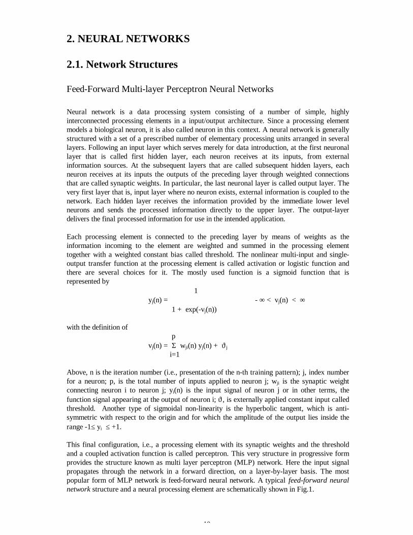
Neural network is a data processing system consisting of a number of simple, highlyinterconnected processing elements in a input/output architecture. Since a processing elementmodels a biological neuron, it is also called neuron in this context. A neural network is generallystructured with a set of a prescribed number of elementary processing units arranged in severallayers. Following an input layer which serves merely for data introduction, at the first neuronallayer that is called first hidden layer, each neuron receives at its inputs, from externalinformation sources. At the subsequent layers that are called subsequent hidden layers, eachneuron receives at its inputs the outputs of the preceding layer through weighted connectionsthat are called synaptic weights. In particular, the last neuronal layer is called output layer. Thevery first layer that is, input layer where no neuron exists, external information is coupled to thenetwork. Each hidden layer receives the information provided by the immediate lower levelneurons and sends the processed information directly to the upper layer. The output-layerdelivers the final processed information for use in the intended application.

Each processing element is connected to the preceding layer by means of weights as theinformation incoming to the element are weighted and summed in the processing elementtogether with a weighted constant bias called threshold. The nonlinear multi-input and single-output transfer function at the processing element is called activation or logistic function andthere are several choices for it. The mostly used function is a sigmoid function that isrepresented by

1 yj(n) = - ∞ < vj(n) < ∞

1 + exp(-vj(n))

with the definition of p vj(n) = Σ wji(n) yj(n) + ϑj

i=1

Above, n is the iteration number (i.e., presentation of the n-th training pattern); j, index numberfor a neuron; p, is the total number of inputs applied to neuron j; wji is the synaptic weightconnecting neuron i to neuron j; yi(n) is the input signal of neuron j or in other terms, thefunction signal appearing at the output of neuron i; ϑ, is externally applied constant input calledthreshold. Another type of sigmoidal non-linearity is the hyperbolic tangent, which is anti-symmetric with respect to the origin and for which the amplitude of the output lies inside therange -1≤ yi ≤ +1.

This final configuration, i.e., a processing element with its synaptic weights and the thresholdand a coupled activation function is called perceptron. This very structure in progressive formprovides the structure known as multi layer perceptron (MLP) network. Here the input signalpropagates through the network in a forward direction, on a layer-by-layer basis. The mostpopular form of MLP network is feed-forward neural network. A typical feed-forward neuralnetwork structure and a neural processing element are schematically shown in Fig.1.

11

ΣOutputLayer nonlinear

neural processing element

Σ

InputLayer

HiddenLayer ΣΣ

Weights w (i,k)

Σ

Fig.1. Schematic representation of a feed-forward neural network

Radial-Basis Function Networks

Another neural network structure similar to the feed-forward neural networks is the Radial-Basis Function Networks. The construction of a radial-basis function (RBF) network in its mostbasic form comprises three entirely different layers. The input layer that is made up of sensorysource nodes. The second layer is a hidden layer of radial base functions. The output layer thatgives the mapping of the input pattern. The transformation from the input space to the hidden-unit space is nonlinear, whereas the transformation from the hidden-unit space to the outputspace is linear. Architecture of a RBF network is shown in Fig.2.

ΣOutputLayer

InputLayer

HiddenLayer

Weights w (i,k)

inputs

basisfunctions

linearoutputs

ΦΦ1 Μ

Fig.2: Architecture of a radial-basis function network

12

Radial-basis function network and the multi-layer perceptrons are examples of nonlinearlayered feed-forward networks. They are both universal approximators. It is therefore alwayspossible to establish a RBF network capable of being accurately alternative to a specified multi-layer perceptron, or vice versa. The differences can be summarized as follows.1. An RBF network has a single hidden layer, whereas MLP network can have one or morehidden layers2. The argument of the activation function of each hidden unit in a RBF network computes theEuclidean norm between the input vector and the center of that unit. On the other hand, theactivation function of each unit in a MLP network computes the inner product of the inputvector and the synaptic weight vector of that unit.

The mapping by the RBF network has the form

Myk(x) = Σ wkj φj(x) + wko

j=1

where M is the number of hidden layer nodes; k, is the index parameter for the output nodes; φj

is the basis function. The biases can be included into the summation by including an extra basisfunction φo whose activation is set to 1. This is similar to the case in MLP networks. For thecase of Gaussian basis functions we have

||x - µj||2φj(x) = exp( )

2σj2

where x is the input vector with elements xi ; µj , is the vector determining the center of thebasis function φj and has elements µji . The Gaussian basis functions are not normalized.

Self-Organizing Neural Networks

Neural networks can learn from the environment, and through learning they improve theirperformance. Multi-layer perceptron networks and radial-basis function networks learn by anexternal teacher which provides the network with a set of targets of interest as this will betermed as supervised learning, and will be explained shortly afterwards. The targets may takethe form of a desired input-output mapping that the algorithm is required to approximate. Inself-organizing systems the network weights are determined by considering the inputinformation only, without recourse to an external teacher.

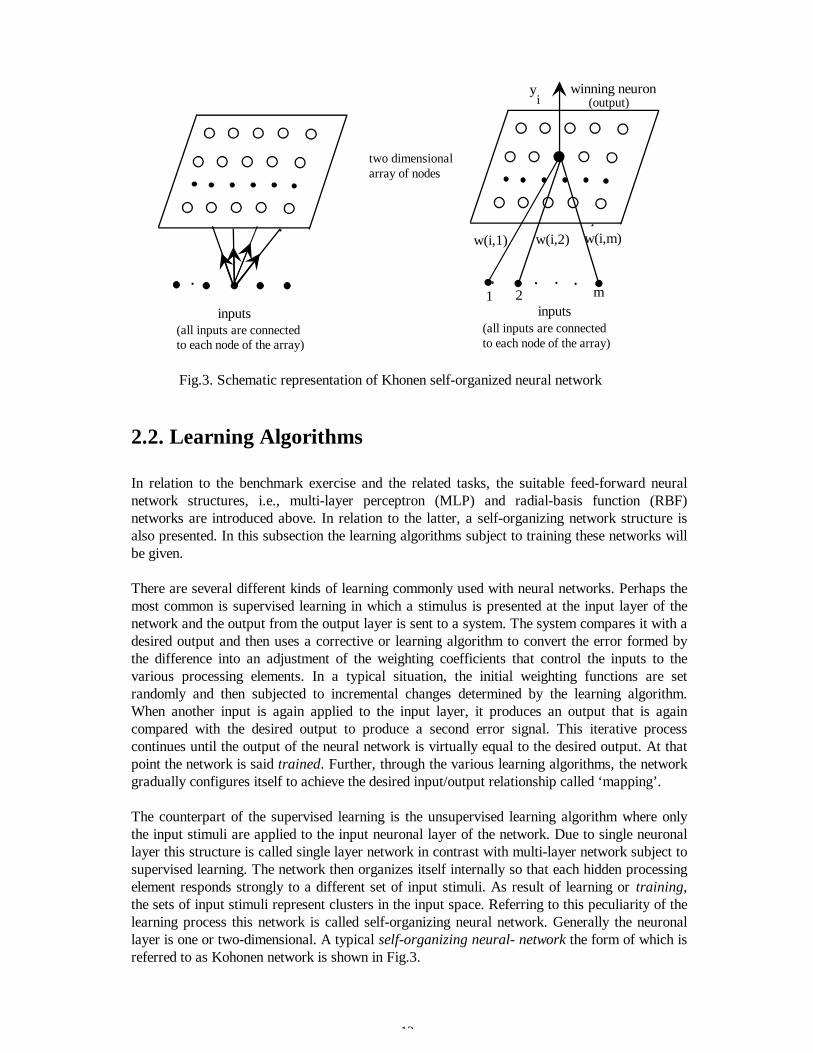
The structure of a self-organizing system may take on a variety of different forms. A mostpopular form consists of an input (source) layer and an output (representation) layer, with feed-forward connections from input to output and lateral connections between neurons in the outputlayer. In another form, it may be a feed-forward network with multiple layers, in which the self-organization proceeds on a layer-by-layer basis to develop a final configuration concerning theweights. The output neurons are usually arranged in a one- or two-dimensional lattice, i.e., atopology that ensures that each neuron has a set of neighbors. An example of such a structure isknown as Khonen model self-organizing network and shown in Fig.3. The Khonen model hasreceived relatively much more attention in implementation. This is because the model possessescertain properties. The associated learning algorithm for this network is called self-organizingfeature map (SOFM) which will briefly be described in the following section.

13

inputs inputs(all inputs are connectedto each node of the array)

(all inputs are connectedto each node of the array)

two dimensional array of nodes

winning neuron(output)

yi

w(i,1) w(i,2) w(i,m)

1 2 m

Fig.3. Schematic representation of Khonen self-organized neural network

2.2. Learning Algorithms

In relation to the benchmark exercise and the related tasks, the suitable feed-forward neuralnetwork structures, i.e., multi-layer perceptron (MLP) and radial-basis function (RBF)networks are introduced above. In relation to the latter, a self-organizing network structure isalso presented. In this subsection the learning algorithms subject to training these networks willbe given.

There are several different kinds of learning commonly used with neural networks. Perhaps themost common is supervised learning in which a stimulus is presented at the input layer of thenetwork and the output from the output layer is sent to a system. The system compares it with adesired output and then uses a corrective or learning algorithm to convert the error formed bythe difference into an adjustment of the weighting coefficients that control the inputs to thevarious processing elements. In a typical situation, the initial weighting functions are setrandomly and then subjected to incremental changes determined by the learning algorithm.When another input is again applied to the input layer, it produces an output that is againcompared with the desired output to produce a second error signal. This iterative processcontinues until the output of the neural network is virtually equal to the desired output. At thatpoint the network is said trained. Further, through the various learning algorithms, the networkgradually configures itself to achieve the desired input/output relationship called ‘mapping’.

The counterpart of the supervised learning is the unsupervised learning algorithm where onlythe input stimuli are applied to the input neuronal layer of the network. Due to single neuronallayer this structure is called single layer network in contrast with multi-layer network subject tosupervised learning. The network then organizes itself internally so that each hidden processingelement responds strongly to a different set of input stimuli. As result of learning or training,the sets of input stimuli represent clusters in the input space. Referring to this peculiarity of thelearning process this network is called self-organizing neural network. Generally the neuronallayer is one or two-dimensional. A typical self-organizing neural- network the form of which isreferred to as Kohonen network is shown in Fig.3.

14

2.2.1. Supervised Learning Algorithms

Back-propagation Algorithm

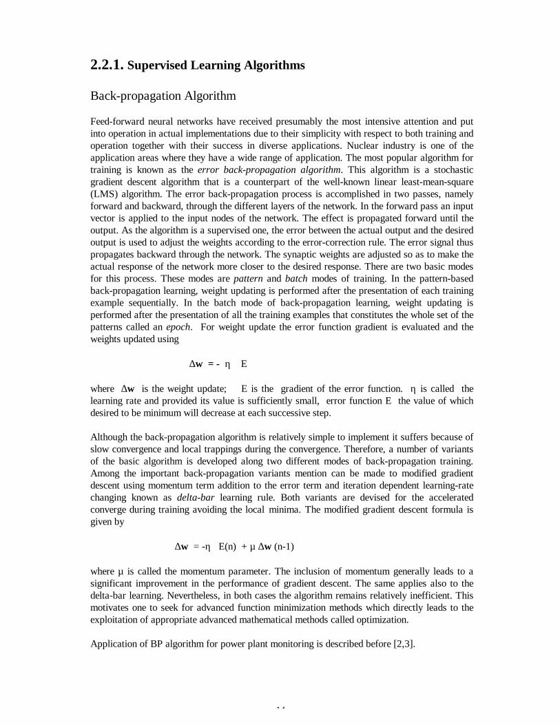
Feed-forward neural networks have received presumably the most intensive attention and putinto operation in actual implementations due to their simplicity with respect to both training andoperation together with their success in diverse applications. Nuclear industry is one of theapplication areas where they have a wide range of application. The most popular algorithm fortraining is known as the error back-propagation algorithm. This algorithm is a stochasticgradient descent algorithm that is a counterpart of the well-known linear least-mean-square(LMS) algorithm. The error back-propagation process is accomplished in two passes, namelyforward and backward, through the different layers of the network. In the forward pass an inputvector is applied to the input nodes of the network. The effect is propagated forward until theoutput. As the algorithm is a supervised one, the error between the actual output and the desiredoutput is used to adjust the weights according to the error-correction rule. The error signal thuspropagates backward through the network. The synaptic weights are adjusted so as to make theactual response of the network more closer to the desired response. There are two basic modesfor this process. These modes are pattern and batch modes of training. In the pattern-basedback-propagation learning, weight updating is performed after the presentation of each trainingexample sequentially. In the batch mode of back-propagation learning, weight updating isperformed after the presentation of all the training examples that constitutes the whole set of thepatterns called an epoch. For weight update the error function gradient is evaluated and theweights updated using

∆w = - η ∇E

where ∆w is the weight update; ∇E is the gradient of the error function. η is called thelearning rate and provided its value is sufficiently small, error function E the value of whichdesired to be minimum will decrease at each successive step.

Although the back-propagation algorithm is relatively simple to implement it suffers because ofslow convergence and local trappings during the convergence. Therefore, a number of variantsof the basic algorithm is developed along two different modes of back-propagation training.Among the important back-propagation variants mention can be made to modified gradientdescent using momentum term addition to the error term and iteration dependent learning-ratechanging known as delta-bar learning rule. Both variants are devised for the acceleratedconverge during training avoiding the local minima. The modified gradient descent formula isgiven by

∆w = -η∇E(n) + µ ∆w (n-1)

where µ is called the momentum parameter. The inclusion of momentum generally leads to asignificant improvement in the performance of gradient descent. The same applies also to thedelta-bar learning. Nevertheless, in both cases the algorithm remains relatively inefficient. Thismotivates one to seek for advanced function minimization methods which directly leads to theexploitation of appropriate advanced mathematical methods called optimization.

Application of BP algorithm for power plant monitoring is described before [2,3].

15

Parameter Optimization Algorithms

As the supervised neural network training can be viewed as a special case of functionminimization, advanced nonlinear optimization algorithms can be applied for that purpose.Among these grid search, line search, gradient search, gradient expansion, conjugate-gradient,quasi-Newton can be referred. These methods all have substantial merits subject to application.The common features of the optimization methods are the followings.

1. Entire set of weights are adjusted once instead of sequential adjustments2. The entire set of patterns to the network is introduced and the sum of all squared errors fromthe patters is used as the objective function.

During the iterative strategy of an optimization method, an appropriate search direction in thespace of the weights is selected. In that direction a distance is moved so that the value of theobjective function is improved when the new values of the weights are introduced into it. Forefficient i.e., fast and effective i.e., avoiding local minima, neural network training, conjugate-gradient and quasi-Newton are of major concern. These are briefly described below.

An essential degree of insight into the optimization problem, and into the various techniques forsolving it, can be obtained by considering a local quadratic approximation to the error function.Let us consider the Taylor expansion of E( w) around some point w* in the weight space

E(w) = E(w*)+(w-w* ) b + ½ (w-w*)T H(w-w*)

where b is is the gradient of E evaluated at w*

b = ∇E

and the Hessian matrix H is defined by

∂E(H)ij = w*

∂wi ∂wj

The local approximation for the gradient is given by

∇E = b + H (w-w*)

For points w which are close to w*, the quadratic approximation is reasonably valid for theerror and its gradient. Consider the special case of a local quadratic approximation around apoint w* which is a minimum of the error function. In this case there is no linear term, since∇E=0 at w*, and therefore the error function becomes

E(w) = E(w*) + ½ (w-w*) H (w- w* )

Consider the eigenvalue equation for the Hessian matrix

H ui = λi ui

where the eigenvectors ui form a complete orthonormal set, i.e .,

uiT uj = δij

16

We expand (w - w*) as a linear combination of the eigenvectors in the form

w - w* = ∑ αi ui

i

so that the substitution yields the error function of the form

E(w) = E(w*) + ½ ∑ λi αi2

iIn this procedure the coordinate system of w is transformed the another one in which the originis translated to, and the axes are rotated to align with the eigenvectors through the orthogonalmatrix whose columns are u.

Since the eigenvectors [ui] form a complete set, an arbitrary vector v can be writtenv = ∑ βi ui

iand therefore we write

vT H v = ∑ βi2 λi

iand so H will be positive definite i.e., vT H v > 0 for all v , if all of its eigenvalues arepositive. In the new coordinate system whose basis vectors are given by the eigenvectors [ui],the contours of constant E are ellipses centered on the origin, whose axes are aligned with theeigenvectors and whose lengths are inversely proportional to the square roots of the eigenvalues.This is illustrated in Fig.4. For a one-dimensional weight space, a stationary point w* will beminimum if

∂E w* > 0 ∂w

The corresponding result is that the Hessian matrix, evaluated at w* is positive definite.

Now, considering the quadratic error function E( w) the local gradient of this error function isgiven by

g(w) = b + H w

and the error function E(w) is minimized at the point w• given the preceding equation, by

b + H w* = 0

Suppose that at step n the current weight vector is w(n) and we seek a particular searchdirection d along which

w(n+1) = w(n) + λ(n) d(n)

and the parameter λ(n) is chosen to minimize

E(λ) = E(w(n) + λ d(n)) .

17

w1

2wu12u

Ellipse

λ12 -1/2λ

-1/2

w*

Fig.4 : Illustration of the coordinate transformation by means ofprincipal component analy sis

This requires that∂∂λ

E(w(n) + λ d(n) ) = 0

which givesgT (n+1) d(n) = 0

that is, the gradient at the new minimum is orthogonal to the previous search direction where g= ∇E. In the successive search, direction d(n) is selected such that, at each step the componentof the gradient in the previous search direction, is not altered so that minimum at that directionis maintained. In particular, at the point w(n+1), we have

gT(w(n+1)) d(n) = 0

We now choose the next search direction d(n+1) such that, along this new direction

gT(w(n+1) + λ d(n+1)) d(n) = 0

holds. If, we expand the preceding expression to first order in λ , we obtain

dT(n+1) H d(n) = 0

where H is the Hessian matrix evaluated at the point w(n+1). If the error surface is quadratic,this relation holds for arbitrary values of λ. Search directions complying with the requirementstated above are said to be conjugate. Approaching to minimum in this way forms the conjugategradient algorithm. We can find a set of P vectors where P is the dimensionality of the weightspace, which are mutually conjugate with respect to H, yielding

dj H di = 0 j ≠ i

This implies that these vectors are linearly independent provided H is positive definite. Hence,such vectors constitute a complete basis set in weight space. Assume we are at some point w1,and we aim to reach to the minimum w* of the error function.

18

The difference between the vectors w1 and w* can be written as a linear combination of theconjugate direction vectors in the form

Pw* - w1 = ∑ αI di

i=1This equation can be re-written recursively as

wj+1 = wj + αj dj

where j-1wj = w1 + ∑ αi di

i=1

In the successive steps, the step length is controlled by the parameter αj. From the aboveequations the explicit solution for these parameters is found to be

djT (b + H w1)

αj = - — — — — — — dj

T H dj

or alternatively dj

Tgj

αj = - dj

T H dj

Following the iterative procedure

j-1wj = w1 + ∑ αi di

i=1

the gradient vector i at the j-th step is orthogonal to all previous conjugate directions. Thisimplies that after P steps the components of the gradient along all directions have been madezero, that is the minimum is reached with the assumption the error surface is quadratic.

The construction of the set of mutually conjugate directions is accomplished as follows.Initially, the search direction is chosen to be the steepest descent, i.e., negative gradient d1 = -g1.Then, each successive direction is chosen to be a linear combination of the current gradient andthe previous search direction

dj+1 = - gj+1 + βj dj

where β is determined substituting this equation into the equation dj H di = 0 that it gives

gj+1T H dj

βj = dj

T H dj

It follows that by means of the successive use of the iterative search direction expression a setof P mutually conjugate directions are generated. Also at the same time dk is given by the linearcombination of all previous gradient vectors

19

k-1dk = - gk + Σ am gm

m=1

Since dkT gj =0 for all k< j ≤ P, we have

k-1gk

T gj = Σ am gmT gj for all k < j ≤ P

m=1

Since the initial search direction is just d1 = - g1, from the equation

gT (n+1)d(n) = 0

above g1T gj =0

so that the gradient at step j is orthogonal to the initial gradient. Further, from here by inductionwe find that the current gradient is orthogonal to all previous gradients

gkT gj = 0 for all k< j ≤ P

The method described above can be summarized as follows. Starting from a randomly chosenpoint w in the weight space, successive conjugate directions are constructed using the parameterβj. At each step, the weight vector is incremented along the corresponding direction using theparameters αj. The method finds the minimum of a general quadratic error function in at most Psteps.

The Conjugate-Gradient Algorithm

In the conjugate-gradient algorithm, the step length is determined by αj and the search directionis determined by βj.. These coefficients are dependent on the Hessian matrix H. However, forthe efficiency of the algorithm the computation of the Hessian is desirable avoided. For thisreason for βj different choices are possible which are obtained from the relationships givenabove. These are

gj+1T (gj+1 - gj)

βj = djT (gj+1 - gj )

or gj+1 (gj+1 - gj)βj = gj

T gj

20

or alternatively

gj+1T gj+1

βj = gj

T gj

These expressions are the equivalent for a quadratic function subject to minimization. In thesame way as βj is calculated without Hessian information, the coefficient αj is calculatedlikewise by

djT gj

αj = - dj

T H dj

This is the expression indicating a line minimization along the search direction dj. The steps ofthe algorithm can be summarized as follows:1- Choose an initial weight vector wo

2- Evaluate the gradient vector go, and set the initial search direction d o = - go

3- At step j, minimize E( wj + αdj) with respect to α to obtain wj+1 = wj + αmin dj

4- Check if the minimum is reached5- Evaluate the new gradient vector gj+1

6- Evaluate the new search direction by computing βj

7- Set j=j+1 and go to step 3

The Quasi-Newton Method

Using the local quadratic approximation, we can obtain directly an expression for the locationof the minimum of the error function. From the quadratic error function

E(w) = E(w) +(w-w•) b + ½ (w-w•)T H(w-w•)

the gradient at any point w* is given by the Newton formula

g = ∇E = H (w - w* )

so that the weight vector w corresponding to the minimum is computed to be

w* = w - H-1 g

Since the quadratic approximation used is not exact it would be necessary to apply thepreceding weight updating iterative, with the inverse Hessian being repeatedly computed at eachnew search point. To avoid this lengthy operations, alternatively, a sequence of matrices G(n)are generated which represent H-1 with increasing accuracy, using the information on the firstderivatives. To ensure that the Hessian is positive definite a special update procedure isdeveloped.

From the Newton formula, the weight vectors at steps n and n+1 are related to thecorresponding gradients by

21

w(n+1) - w(n) = - H-1 (g(n+1) - g(n) )

which is known as the Quasi-Newton condition. Assuming H is constant in the neighborhood ofa minimum, we can write

∆wo - ∆w = -H-1 gn+1

Above, ∆wo is the weight increase required to reach the minimum, and ∆w is the actual weightincrease. Since H is not constant, ∆w above cannot be directly calculated. Therefore for theevaluation of H-1, a symmetric non-negative definite matrix G is considered which is inparticular is to be positive if there are no constraints on the variables and might initially be aunit matrix. This matrix is modified after the i-th iteration using the information gained bymoving down the direction

∆wi = -Hi gi i= 1,2,...,N

in accordance with the equation before the preceding one. This direction points towards theminimum of the error function. The commonly used update formula is the Davidson-Fletcher-Power algorithm where, while moving down to the minimum, the line minimization isperformed, as it is the case for conjugate-gradient method. Therefore the method is calledvariable-metric minimization. The basic procedure for the quasi-Newton method is as follows.

1- A starting point is selected

2- define σI = αI ∆wi

3- set the weight values as wk+1 = wk + σI i=1,2,.....,N

4- evaluate E(wk+1) and gk+1

5- define yk = gk+1 - gk

σk σkT Gk yk yk

T Gk

Ak= , Bk=- σk yk yk

T Gyk

and evaluate the matrix G k+1 by setting

Gk+1 = Gk + Ak + Bk

6- Set k=k+1 and start from step 2, repeat the iteration until the minimum is reached.

The advantages of quasi-Newton (variable-metric) method can be stated as follows.- Use of second derivative ( Hessian) matrix makes the method the most robust optimizationmethod avoiding local optima- Relatively few iterations for convergenceThe method is ideally suited for neural network training with orthogonal input variables, e.g.,with principal component scores.

Application of optimization algorithms to neural network training for power plant monitoring isdescribed before [4]

22

Kalman Filtering Algorithm

The supervised training of a multi-layer perceptron is an adaptive nonlinear optimizationproblem for system identification. The function subject to minimization is the function of errorthat is the measure of deviations of the network outputs from desired or targets outputs. It isexpressed as a function of the weight vector w representing the synaptic weights and thresholdsof the network. The standard back-propagation algorithm is a basic optimization algorithm.With its simple form its convergence properties are relatively poor concerning speed andtrappings at the local minima. To improve its convergence properties alternative approaches areimplemented borrowing techniques from advanced adaptive non-linear least mean squareestimation. These techniques are collectively referred to as recursive least-squares (RLS)algorithms that are the special case of the Kalman filter. Since the Kalman filter equations arefor linear systems, in the neural network training this linear form should be modified. Thismodified form is known as extended Kalman filter and briefly described below.

Kalman filtering can be used for adaptive parameter estimation as well as optimal stateestimation for a linear dynamic system. In the application of Kalman filtering to neural networktraining the parameters are the network weights which are considered as states and theestimation of the states is performed using the information applied to the network. However thisinformation cannot be used directly as the size of the covariance matrix is equal to the square ofthe number of weights involved. To circumvent the problem we partition the global probleminto a number of sub-problems where each is at the level of a single neuron. Then, with theexclusion of the sigmoidal non-linearity part, the model is linear with respect to synapticweights. Now, we consider neuron i, which may be located anywhere in the network. During thetraining, the behavior of neuron i represent a nonlinear dynamical system so that the appropriatestate and measurement equations are

wi (n+1) = wi (n)

di (n) = ϕ (yiT(n) wi (n)) + zi (n)

where the iteration n corresponds to the presentation of the n- th patter; yi (n) is the input vectorof neuron i; ϕ (x) is the sigmoidal non-linearity. In the Kalman filtering zi(n) is the measurementnoise which is assumed to be Gaussian white for the optimality. The weight vector wi of theoptimum model for the neuron i is to be estimated through training with patterns.

For linearization, the measurement equation is expanded to Taylor series about the currentestimate wi (n) and linearized as

ϕ[yiT(n)n wi(n)] ≈ qi

T(n) wi(n) + {ϕ[yiT(n) wi(n) - qi

T(n) wi(n)}

where∂ϕ[yi

T(n) wi(n)]q(n) =

∂wi (n) wi(n)=wi(n)

that results in for a sigmoid function

q(n) = oi(n) [1- oi(n)] y(n)

23

where oi(n) is the output of neuron i corresponding to the weight estimate wi(n); y(n) is theinput vector. In the Taylor expansion the first term at the right hand side represents thelinearization and the second term is the modeling error. Neglecting the modeling error we arriveat

di(n) = qiT (n) wi (n) + zi(n)

In the RLS algorithm, the measurement error zi(n) is a localized error. The instantaneousestimation of it is assumed to be

∂E(n)zi(n) = -

∂oi(n)

where E(n) is the error function defined by

E(n) = ½ Σ [dj - oj]2

j∈O

where O represents the neural network output space. The resulting solution is defined by thesystem of recursive equations of the standard RLS algorithm that are

Qi(n) = λ-1 Pi(n) q(n)

Qi(n)ki(n)=

1+ QiT(n) q(n)

wi(n+1) = wi(n) + zi(n) ki(n)

Pi(n+1) = λ-1 P(n) - k(n) QiT(n)

where n is the index parameter of iteration, each iteration being the introduction of oneindividual pattern from an epoch. Pi(n) is the current estimate of the inverse of the covariancematrix of q(n), and k(n) is the Kalman gain. The parameter λ is a forgetting factor less butcloser to unity. The very last equation above is called Riccati difference equation. With theabove recursive algorithm each neuron in the network receives its own effective input q(n)thereby possesses its own covariance matrix Pi(n).

In the actual Kalman algorithm in contrast with the exponential weighting of all estimationerrors, a process noise is introduced in the state equation as

wi (n+1) = wi (n) + vi (n)

where vi(n) is the process noise which is white and assumed to be Gaussian for optimality. Inthis case the solution of the system equations presents a solution similar to those from RLSestimation as

24

wi (n+1) = wi(n) + Ki(n) [di(n) - qiT (n) wi (n) ]

Qi(n) = Pi(n-1) + R(k-1)

Qi(n) q(n)Ki(n) =

Z(k)+q(n)T QiT(n) q(n)

Pi (n) = Qi(n) - Ki(n) Qi(n)

where R and Z are the auto-covariance matrices of the process noise and measurement noise,respectively; Ki(n) is the Kalman gain; Pi(n), is the error covariance matrix indicating thevariances of the estimated parameters. The difference di(n) - qi

T (n) wi (n) is called innovationand is easily computed for the output neurons. However for the hidden layer - ∂E(n)/ ∂oi(n)can be used to replace the difference appearing in the state equation during the iterative period.

Kalman algorithm is relatively superior to other type of learning algorithms since it is a model-based algorithm and the modeling errors are counted in the measurement errors. On the otherhand, the learning process during the neural network training is a stochastic process and thiswill be shown shortly afterwards. The process noise in the model considers the stochastic natureof the learning process and thereby it plays important constructive role on the convergenceproperties of the adaptive process. Due to these features of Kalman filtering, the convergence ismuch faster and undesirable excessive learning called memorizing incidents in neural networktraining is avoided as the memorizing badly deteriorates the generalization capability of thenetwork. Additionally, the fast learning capability and ability of modeling stochastic signalsmake the Kalman filtering algorithm essential learning algorithm for using the neural networksfor stochastic signal processing. Application of Kalman filtering algorithm to neural networktraining for power plant monitoring is described before [5,6].

To see the stochastic nature of the learning process consider a vector x of independent variablesand a scalar d which is independent variable. If we have N measurements of x, we have x1, x2,......, xN and correspondingly d1,d2,...., dN . The neural network model is expressed by

d = g(x) + ε

where g(x) is some function of the vector x and ε is random expectation error. In this model,taking the expectation of both sides, the function g(x) is defined by

g(x) = E[d|x]

The conditional expectation defines the value of d that will be realized on the average given aparticular realization of x. Let the actual response of the network is defined by

y = F(x,w)

where w represents the synaptic vector. The synaptic weight minimization for the cost functionJ(w) used in neural network training

J(w) = E[(d - F(x,w))2]

would also minimize the multiple integral

25

E[(g(x) - F(x,w))2] = ∫ f(x) [g(x) - F(x,w)]2 dx

where f(x) is the probability density of x and note that, the function subject to minimization is arandom variable. This result therefore, indicates the statistical nature of the learning processeven though the different patterns of a particular realization of x are deterministic. From theprobability theory viewpoint, the difference between the input-output pairs of x used for thetraining obeys an arbitrary distribution f( x) and therefore do not take a functional relationshipbetween input and output deterministically. f (x|w) being the density function parameterized byw, the model f( x|w) with good generalization capability should approximate the true distributionf(x). In other words, the learning is dependent on the probability density of the input vectorwhere the network performance should not depend on the network structure, i.e., f( x|w)=f(x). Itshould only be dependent on the statistical properties of the input vector itself, if the appropriatenetwork model is used for training.

2.2.2. Unsupervised Learning Algorithms

Self Organizing Feature Map Network

Feature mapping converts patterns of arbitrary dimensionality into the responses of one or two-dimensional arrays of neurons called feature space. A network that performs such a mappingand the related algorithm are referred to as feature map and self-organizing feature mapping(SOFM), respectively. These networks are based on competitive learning where the outputneurons of the network compete among themselves to be activated so that only one outputneuron is on at any one time. The output neurons that win the competition are called winner-take-all neurons. In addition to achieving dimensionality reduction, also topology-preservingmap that represents the neighborhood relations of the input patterns is obtained. That is, thesimilar patterns in some sense should give outputs topologically close to each other. The outputlayer in this map commonly one or two-dimensional virtual array in the form of a lattice.Different input features are created over the lattice. Each component of the input vector x isconnected to each of the lattice nodes as shown in Fig.3. To describe the SOFM algorithm theinput vector x =[x1, x2,......,xp]T and the synaptic weight vector of neuron j , w =[wj1, wj2,........,wjp]T, j=1,2,..., N , is considered. n is the total number of neurons. To find the best match ofthe input vector x with the synaptic weight vectors wj , we compare the inner products wj

Tx forj=1,2,...,N and get the largest. In the formulation of an adaptive algorithm, it is convenient tonormalize the weight vector wj to constant Euclidean norm. In this case the best matchingcriterion is equivalent to the minimum Euclidean distance between vectors.

One approach to training a self-organizing feature map network is to use the Khonen learningrule with updated weights going to the neighbors of the winning neuron as well as to thewinning neuron itself. The topological neighborhood of the winning neuron i is shown in Fig. 5and it is represented as Λi (n) indicating its discrete time (iteration) dependence.

26

Λi=

Λi=

Λi=

0

1

2

Λi= 3

Fig.5: Square topological neighborhood Λ around winning neuron iat the middle

The basic self-organizing learning algorithm can be summarized as follows.

1. Initialization. Choose random values for the initial weight vectors wj (0)

2. Select Pattern. Draw a pattern x from the input patterns formed by a set of sensory signals

3. Similarity Matching. Find the best matching, that is, winning neuron i(x) at time n, using theminimum-distance Euclidean criterion:

i(x) = argj min || x(n)- wj|| , j=1,2,...,N

where N is the number of neurons in the two-dimensional lattice.

4. Updating. Adjust the synaptic weight vectors of all neurons, using the update formula

wj (n) + η(n) [ x(n) - wj (n)] j ∈ Λi (n)

wj (n+1) = { wj (n) otherwise

for the winning neuron where η(n) is the learning-rate parameter; Λ(n) is the neighborhoodfunction centered around the winning neuron i(x) and it is illustrated in Fig.5.

5. Continuation. Return to the step 2 and continue until no noticeable changes in the featuremap are observed.

27

With this learning rule, nearby nodes receives similar updates and thus end up responding tonearby input patterns. The neighborhood function and the learning constant η are changeddynamically during learning. As result of the of weight adjustment, a planar neuron map isobtained with weights coding the stationary probability density function p( x) of the patternvectors used for training. The ordered mapping of patterns establishes the weights indicated wij.The self-organizing learning process is stochastic in nature so that the accuracy of the mapdepends on the number of iterations of the SOFM algorithm. Also, the learning parameter η andthe neighborhood function Λi are critical parameters. That is their appropriate selection isessential for satisfactory performance after the training.

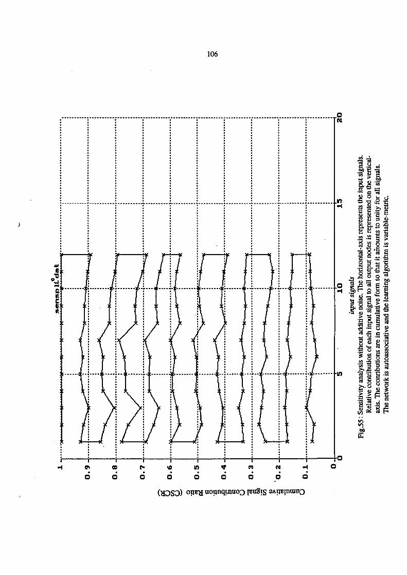
2.3. Sensitivity

Sensitivity analysis investigates the effect of changes in input variables on output predictions. Itis based on the perturbation of a system parameter at a point of interest in the form of partialderivatives ∂yj/∂xi where yj represents the j- th network output and xi represents i-th networkinput where y is expressed by

yj = f(x1, x2, ........., xn)

Also one can define dimensionless sensitivity coefficient ( dy/y)/(dx/x) which represents ratio ofthe percentage changes in the parameters. Sensitivity is a measure of contribution of an input tolet the network recognize a certain pattern in a non-temporal neural network application wherethe input-output mapping is static. That is both the input vector x and the output vector y arerepresent spatial pair of patterns that are independent of time as this is the case with thebenchmark data. Ideally, the relative sensitivities of each network’s input-output pair aredesired to be about the same for the robustness of the network. A robust network is one thatestimates the correct output for a respective input that contains an error or missing data,without degrading the output estimates of the other parameters at the network’s output. Toachieve robustness, certain degree of noise is superimposed on training data set. In this case thetraining set gains some probabilistic features subject to estimation. Referring to this, acommonly used probabilistic sensitivity measure that relates to input and response probabilitydistributions in terms of the standard deviations is (d σy/dσx). The importance of this due to theinformation it provides on the degree of response uncertainty or variability reduction as afunction of reduction of the input uncertainty. Similarly, a probabilistic measure associated witha change in the mean value is useful in examining the effect of the uncertainty in the mean valueof an input random variable. Probabilistic sensitivity measures identify essential inputparameters that contribute to the uncertainty in the estimation of the network. The relativeimportance or ranking of input random parameters can be used in making decisions leading touncertainty reduction.

3. ANALYSIS OF THE RESULTS REPORTED

The benchmark analysis results are globally presented at SMORN VI, in the form of anextended summary where also the analysis results of the benchmark organizers are illustrated.The full documentation of the related Extended Summary Report is given in the appendix A andthe report has also been documented in a recent OECD-NEA publication [7]. In this section theanalysis of the results reported by the participants are presented. The presentation comprises aconcise description of the documented results sent by the participants pointing out also the key

28

features. For the detailed information on any of these descriptions reference is made to the fulldocumentation which is included in the Appendix B. Below, is the concise evaluation of thesubmitted reports where the presentations are in alphabetic order referring to the respectivecountries.

1. H. Mayer, P. Jax and U. Kunze (Germany)

The participants used an algorithm coded in C ++ and developed by them. The extensive analyseshave been performed and their results are reported. For training the network standard back-propagation algorithm for multi-layer perceptrons (MLP) networks is used. For the prescribednetwork structures different back-propagation learning strategies i.e., variation the learning rateη and momentum rate µ, are employed. From the benchmark analysis submitted, the followingobservations are made- Various activation-functions for neurons are employed. These are, Sigmoid Fermi Function,Limited Sine Function, Unipolar Ramp Function, Gaussian Function.

- Standard back-propagation algorithm with some learning variants is employed. These aremainly

• Super SAB• Delta-bar-delta• Resilient Back-propagation

- In addition to the standard back-propagation algorithm, some variants of this algorithm arealso exercised where insufficient or no convergence was obtained. Among these are

• Zero-point search method• Batch learning in constant η• Learning with adapted global η• AMBP learning• Quickprop (back-propagation) learning

- The highest convergence rate and best generalization are achieved with the inputs when• Error function is based on L 2-norm• Each active neuron receives a constant excitation that is also subject to weighting,

i.e., threshold• Excitation is achieved in on-line learning by stochastic presentation of each pattern

with an epoch- Input and output signal normalizations are performed between 0 and 1- Errors are expressed as deviations- Basic sensitivity analysis is considered

The extensive study results are reported and they indicated that the participant have endeavoredto have thorough understanding of back-propagation neural network performance by using theactual plant data and they carried out researches beyond the formal benchmark analysis tasks;repeating the analyses with all available signals, for example. Their results are among theoutcomes of high performance category, considering the reported benchmark results ofparticipants in perspective. The standard back-propagation (BP) learning algorithm is ratherpopular because of its simplicity. However it has rather poor final convergence properties,although the initial convergence properties are satisfactory, and therefore it needs a lot ofelaboration during training. The elaboration is carried out and therefore extensive analysisresults are obtained. The deviations of the estimated signals by the network from the actualvalues are relatively small and generalization capability is quite satisfactory. However, someBP learning strategy might still improve them. This learning strategy should still be a dynamic

29

one as far as the learning parameters are considered in a BP approach. Although themathematical treatment is somewhat involved, basically, due to the learning process is astochastic process, the stochastic presentation of the training examples should be randomized(shuffled) from one epoch to other for better performance of BP algorithm. This general resultis also verified experimentally in the reported research. Although several variants of the BPalgorithm are investigated, any recommended reference to one of them among the others is notmade for eventual condition monitoring applications.

2. U. Fiedler (Germany)

The participant used a commercially available NeuralWorks II/Professional Plus algorithm byNeuralWare, Inc. From the benchmark analysis report submitted, the following observations aremade

- Normalization is performed and bipolar inputs are used- Standard back-propagation (BP) algorithm is used with sigmoid activation function.Momentum term is included into the learning algorithm although momentum coefficient isrelatively low and learning parameter is high. Learning parameter is decreased in the advancedstage of learning.- Errors are reported as root mean square (RMS) and MAX-error in % in contrast withdeviations from the nominal value.

From the inspection of the results reported it is to conclude that, the additional elaboration onthe training strategies would be suggested to improve the reported results.

3. Y. Ding (Germany)

The participant used a self-developed algorithm in Window environment. From the benchmarkanalysis report submitted, the following observations are made

- The neural network in use is especially designed for false alarm reduction in a monitoringtask. However it is modified for the present benchmark.- Normalization is made between 0 and 1 but 10% over ranging- The order in which the examples are presented to the network is randomized- Relatively high learning rates are used

The results reported indicated the global convergence ability of the algorithm used. However,the deviations between the network estimates and the nominal input counterparts at some partsof the learning period are relatively high and this can be improved by carrying out someelaborated learning strategies. Especially, the modification of the learning parameters, i.e.,learning rate η and the momentum coefficient α during the learning process should be varied forenhanced training. Increased training patterns gave better results for the training ranges as wellas the ranges beyond the prescribed training ranges. In spite of overall satisfactory performanceof the network used, a better performance requirement for this network in critical applications ismainly attributed to the original design of the network that is tuned for the benchmark analysis.Additional elaboration on the training strategies would apparently improve the reported resultsfor a desirable level of performance.

30

4. S. Thangasamy (India)

The participants used an algorithm in C language in UNIX environment. From the benchmarkanalysis report submitted, the following observations are made

- The algorithm makes use of a sigmoid function.- Batch mode of training is implemented. In the batch mode of learning, weight updating isperformed after the presentation of all training examples that constitutes an epoch.- The cost function which is conventionally sum of the squared errors divided by the number ofpatterns is further divided by the number of neurons to obtain an average square error perneuron. The latter is used to determine the success of training and terminate the process ofoptimization over the weight space.

- Maximum number of iterations is also used as a parameter to help intervene duringoptimization in situations of very low error thresholds or the nature of the problem leading topoor convergence.

The results reported indicated the global convergence ability of the algorithm used. However,the deviations between the network estimates and the nominal input counterparts at some partsof the learning period are relatively high. Increased training patterns gave better results for thetraining ranges as well as the ranges beyond the prescribed training ranges. In spite of overallsatisfactory performance of the network used, a better performance requirement for thisnetwork in critical applications is mainly attributed to the normalization of the data,presentation of the patterns to the network and the static nature of the learning parameters ηand α. Additional elaboration on the training strategies would apparently improve the reportedresults.

5. G.S. Srinivasan and Om Pal Singh (India)

The participants used back-propagation algorithm. Among the basic benchmark tasks, multi-input single-output structure was subject to study and the relevant results are reported. Fromthe benchmark analysis report submitted, the following observations are made- Sigmoidal activation function was assigned at the neural nodes- The initial weight values were randomly chosen from sampled background noise of steamgenerator environment of a fast reactor. The weight values were normalized between -1 and +1.- Momentum term in learning algorithm was not employed and still fast convergence is reported.The results reported indicated the global convergence ability of the algorithm used. However,deviations between the network estimates and the nominal input counterparts at some parts ofthe learning period and for some certain signals are relatively high and vice versa. This isattributed to the initial weight selection strategy and the missing momentum term in learning.The function of the momentum term during learning is twofold. One is that it acceleratesdescent in steady downhill directions. The second is that it prevents the learning process fromterminating in a shallow local minimum on the error surface in the multidimensional space. Theinitialization of the synaptic weights and threshold levels of the network should be uniformlydistributed inside a small range. This is because to reduce the likelihood of the neurons in thenetwork saturating and producing small error gradients. However, the range should not be madevery too small, as it can cause the error gradients to be very small and the learning therefore tobe initially very slow. Additional elaboration on the training strategies would apparentlyimprove the reported results.

31

6. M. Marseguerra and E. Padovani (Italy)

The participants have submitted a detailed analysis report of the benchmark tasks theyexecuted. They used an algorithm of their own coding. The neural network (NN) trainingperformed with the back-propagation (BP)-algorithm as follows.

• The initial values of the connection weights wij are randomly chosen in the interval -0.3, +0.3.

• Batch training mode is employed where the wij are updated after each batch of 10training patterns.

• Each batch of training patterns is repeatedly (15 times) presented to the network.• The whole training lasts N batches, each repeated 15 times. Thus the network

receives a total of 10x15xN training patterns and its weights are updated 15xN times. A typicalfigure for N is selected to be N=1.6 10 5.

• After the 15 repetitions of each batch (and therefore after 15 updating of the weights)the learning and momentum coefficients are varied according to a sigmoid function from theinitial values αo and ηo to zero.

• The initial values αo and ηo relating to the neural network for generated electric power(GEP) estimation are 0.7 and 0.3, respectively. Those for the auto-associative NN are 0.5 and0.6, respectively. The above values have been selected over a two-dimensional grid of pointswithin the unit-square.From the benchmark analysis report submitted, the following observations are made.- The cost (error) function subject to minimization is the square of the difference between thedesired and the computed (estimated by NN) output, averaged over the training set, i.e., numberof patterns in one epoch.- Normalization of the signals is performed between 0.2 and 0.8.- Errors between the estimated values and their counterparts are expressed in terms ofdeviations.- Sensitivity analysis is performed in great detail and a substantial discussion is presented. Theyare reported as a set of the partial derivatives of outputs with respect to inputs.

Since neural network is a non-linear device, the sensitivities, besides depending on the synapticweights that are constant once the NN is trained, also depend on the particular input pattern.Therefore, it should be expressed as an average value considering all input-output pattern pairsforming an epoch. Generally, a data set involving a set of input-output pairs and being used afeed-forward neural network training does not contain all the information about the dynamicsystem where the set comes from. Therefore the sensitivities between input and output representindividual neural network attribution for the signals in use rather than those representing theplant-sensitivity. For robust training these attributions are approximately expected evenlydistributed and independent of the initial point used to start training. The verifications on thesensitivity considerations are successfully carried out in this benchmark report with fruitfulrelevant discussions. The results reported indicated that the participant have endeavored to havethorough understanding of back-propagation neural network performance by using the actualplant data and they carried out researches beyond the basic benchmark analysis tasks andextended to optional tasks. Their results are among the outcomes of high performance category,considering the reported benchmark results of participants in perspective. The deviations of theestimated data by the network from their actual counterparts are relatively small andgeneralization capability is quite satisfactory. However, by some back-propagation learningstrategy they can still be improved. This learning strategy should still be a dynamic one as faras the learning parameters are considered in a BP approach.

32

7. K. Nabeshima (Japan)

The participant has submitted his benchmark analysis results, all the prescribed benchmarktasks having been performed. Additionally, he gave his results on the sensitivity analysis. Heused a code originally developed for on-line plant monitoring where the network graduallychanges its characteristics by updating the weights. Standard BP algorithm with sigmoidal non-linearity and momentum term was employed in his analysis where both input and output signalsare normalized to be in between -0.5 and +0.5 for inputs and 0.1 and 0.9 for the output signals.He reported the weight values and the learning errors of the trained networks used for thebenchmark tasks together with the minimum and maximum estimated signal values for eachcase. He repeated the similar experiments not only for the prescribed network structures for thebenchmark but also using various number of hidden layer nodes as optional investigation forfinding optimal number of hidden layer nodes in each case, starting from five. He reported both,the global training error and the corresponding error in the test (recall) phase outcomes. Thiswas carried out for both, auto-associative and hetero-associative cases aiming to obtain a betternetwork performance. Training errors decreased with the increasing number of hidden layernodes although this was not the case for the recall-phase outcomes that it makes the caseinconclusive. He eventually concluded that the number of hidden layer nodes is not a sensitiveparameter for learning. However, since the learning error is not the only factor for thedetermination of the performance, further elaboration on this issue is needed.

He carried out sensitivity analysis using the ratio of finite variations of the signals in place ofanalytical derivatives. The sensitivity results are rather uneven indicating some need ofconsideration on this issue as the even signal contributions are desirable for a better networkperformance. Because of gross computation of the derivatives, some additional errors mighthave affected the results.

Following the training, the reported errors are rather small so that, his detailed reported resultsare expectedly quite satisfactory while the results are among the outcomes of high performancecategory, considering the reported benchmark results of participants in perspective.

8. Dai-Il Kim (Republic of Korea)

The back-propagation algorithm used in this participation is coded in C and run in a Pentium-90 computer. The activation function considered is a bipolar function with a constant slope. Theslope is 1.0 for output neurons and 0.8 for the hidden neurons.From the benchmark analysis report submitted, the following observations are made.- Normalization of the signals was performed between -0.5 and +0.5.-Constant learning rate is employed where η=0.068- Errors between the estimated values and their counterparts are expressed in terms ofdeviations.- No momentum term is employed.- Some optional tests are performed for the robustness verification of the network and thesensitivity analysis is employed for this process.The results reported indicated the global convergence ability of the algorithm used. However,the deviations between the network estimates and the nominal input counterparts at some partsof the learning period and for certain signals are relatively high and vice versa. This isattributed to the constant learning rate and the missing momentum term in learning. Thefunction of the momentum term during learning is twofold as was explained before. Robustnessof a neural network can be defined as the stability of the learning process being independent ofthe starting point of the learning process in the multidimensional parameter space. Additionally,

33

the sensitivities are desirably expected approximately evenly distributed. In this contribution therobustness verification is performed with the help of sensitivity analysis. To this end, theinvestigations are extended to the network of 12:14:12 structure apart from the nominal auto-associative network of 12:8:12 structure prescribed in benchmark task execution. Thesensitivities reported are rather uneven and rather low. Additional conventional elaboration onthe training strategies would apparently improve the reported results.

9. E. Barakova (The Netherlands)

The standard back-propagation algorithm is used in this participation. For this, commercialsoftware called ‘InterAct’ is employed. Because of the limitations of the available software, thebenchmark data was considered to be a temporal data and accordingly very limited analysis wasperformed with temporal processing. However the benchmark data at hand is a combination ofdifferent operations at different times and the data sets are the in the form of patterns to apply tothe neural network as spatial input patterns rather than temporal sequences. Therefore thedeviations between the estimated signal values and the given counterparts are reported to berelatively high, as one should expect.

Temporal processing requires that the neural network should have dynamic properties thatmakes it representative to time-varying signals. For this purpose, time delays are introduced intothe synaptic structure of the network and to adjust their values during the learning phase. Sincethe benchmark tasks concern only spatial learning process in contrast with temporal (time-dependent) learning process the reported results are to be considered and re-reportedaccordingly.

4. FURTHER STUDIES WITH THE BENCHMARK DATA

In this section some further analyses carried out with the benchmark data will be presented.These include advanced learning algorithms and the sensitivity analysis and they are given in thefollowing subsections.

4.1. Advanced Learning Algorithms

As it is noted from the reported benchmark results, all participants used the standard back-propagation (BP) algorithm as a basic training algorithm. However, as it was pointed outearlier, this should be replaced with more advanced training methods to enhance the training. Incorroboration with these statements, it is interesting to note that although the training algorithmis the same and basic one, there is rather big performance difference among the reported results.This is because of the selection of the parameters and necessity of their modification duringtraining while a systematic approach for such a treatment cannot be prescribed in advance asthis is dependent on the data and the circumstances. The essential algorithms for this purposeare described in some detail in the preceding section. With respect to this, some additionalstudies have been carried out. In this context, some direct results together with the associatedresults obtained with the implementation of these algorithms are presented below.

The benchmark data analysis results obtained by BP algorithm were presented earlier and theyare illustrated in the extended summary report [8]. In this study, advanced nonlinearoptimization methods for training together with the enhanced sensitivity analyses areconsidered. Additionally, to emphasize the generalization capability of these algorithms the

34

reported analyses here are carried out also slightly different than those carried out forbenchmark standard benchmark tasks. In particular, in the benchmark task for the auto-associative neural network with multiple signal data, the training is carried out for initial 600patterns. The associated recall was performed for the total number of patterns of 1169 incontrast with 942 patterns used in the standard benchmark task (in place of 1169 patterns inTask a-1).

To begin with, the results obtained with the BP algorithm are given in Fig.6 where the learningis carried out first 1000 patterns and the task is designed to be BB-1. In this analysis, a set ofuncorrelated random data, i.e., noise, is imposed on the benchmark data. The effect of this noiseintroduction on the data can be explained in the following way. Since the benchmark data isobtained from actual power plant, it contains measurement errors. During the network trainingthis measurement errors affect the training and degrade the learning performance. In the extremecase these errors are also learned where this situation is termed as memorizing. To avoid this,the learning process should be limited in the case of working with measurement data. Onemethod for this limitation is the random data introduction to the data. As result of this, themeasurement errors are not traced in the learning process of the network and the net result issome reduction of the estimation errors by the network. This result is seen in Fig.6, where thestandard deviation of the noise introduced on a signal is equal to the 5% of the maximum valueof the respective signal among the total number of patterns and the standard deviation is keptconstant for that signal throughout the patterns. Attention is drawn that, by the noise additionthe estimation errors by the network are slightly reduced, for the cost of missing some minordetails also available in the given data. In connection with this, reference is particularly made toone of the peculiarities present in the benchmark data, the peculiarity being the rinsingoperation. This operation is generally done for thermal performance enhancement and this isincluded into the benchmark data twice consecutively but in opposite phases as this is seen inpatterns around 800. This particular operation belongs to the normal operation while theoperational conditions are slightly different than those involved during routine operation. Thetrained neural network without the rinsing-process experience is expected not to follow thisunknown operation. However, in this case the difference between the estimated signal value andthe signal itself would be relatively large so that this particular operation is detected. This isclearly seen in the illustrations of the benchmark analyses. Referring to this detail, the noiseintroduction to the data partly obscures the identification of this detail. However, thisconsequence can be assessed positively since the rinsing process belongs to normal operationand the estimation error should not be big as that could lead to reporting false alarms. Thetrade-off between these two considerations should be kept in view. In the framework of thepresent study, the other implications of the noise introduction on data will be illustrated shortlyafterwards in connection with sensitivity. A similar test as above but taking 600 patterns forlearning is given in Fig.7 where the task is designed to be BB-2. To show the signals and thesuperimposed noise magnitude involved in scale together, the same analysis above is illustratedagain in Fig.8 where the task is designed to be b-1. In Fig.8 particularly, in place of theestimated patterns, the patterns introduced at the neural network input are presented. The errorsseen in the figure are irrelevant but they are there because of the plotting routine bay thealgorithm used for plotting and therefore the errors are to be out of concern and subject toomission in this particular case. However, here a point noteworthy to mention is the peculiarityof the operation represented by the patterns after 942. This operation is termed as stretch-outand briefly described blow in connection with the further analyses. Referring to the stretch-outoperation, during the learning process using the patterns up to 1000, this particular operation isexplicitly included into the training. The resulting corresponding estimation i.e., estimationbeyond the pattern 942, by the network is much improved relative to those obtained using thepatterns until 942 from the beginning, for learning. The implications of this difference ispresented below together with the further analyses related.

35

The analyses are carried out using the advanced training algorithms as these algorithms aredescribed in the preceding section. These are namely, nonlinear optimization algorithms,Kalman filtering algorithm and radial-basis-functions (RBF) network algorithm (self-organizingand orthogonal-least-squares). In this context, some illustrations of auto-associative benchmarkdata analysis results with variable-metric nonlinear optimization algorithm are shown in Fig.9where the task is designed to be C-2. The range of training spans first 600 patterns of the dataset and recall is carried out over the total number of patterns, i.e., 1169. The back-propagationcounterparts of this analysis are reproduced here for convenience in Figs.10 and 11 while theyare presented in the extended summary report [7] earlier ( Benchmark Tasks a-1 and a-2). Thecounterpart benchmark tasks are in the form of two analyses in place of one due to the range ofthe analyses; namely, in the Task a-1, the learning spans first 600 patterns and thecorresponding recall is carried out over 942 patters from the beginning. In the Task a-2, thelearning spans first 1000 patterns and the corresponding recall is carried out over the total 1169patterns. In addition to the first peculiarity of the data described above, here the attention isespecially drawn to the second peculiarity which concerns a particular plant operation in theform of extended plant operation which is referred to as ‘stretch-out’. This type of operation isquite peculiar to the PWR plant from which the benchmark data prepared. This operation isperformed towards the end of the fuel-cycle to extend the plant operation for some time.Referring to the first principle of the Thermodynamics, this is accomplished by keeping thetemperature difference between the hot-leg and cold-leg about the nominal range although therespective temperatures themselves are below their nominal ranges. In this respect, the operationbelongs to the category of normal operation and the major differences between the operation inthe course of fuel cycle and at the end of the cycle are the temperatures as far as the neuralnetwork is concerned. Because of this very reason, in the benchmark, in place of individual hot-leg and cold-leg temperatures, the differences (two differences because of two primary loops)are considered for training and thereby the major difference between the operations have beeneliminated. The basic implication of this is that the total set of benchmark data being consideredis expected to be appropriate representative of one complete fuel-cycle power plant operation,the data being made exclusively suitable for training for the purpose of plant monitoring byneural networks. From the inspection of Fig.9, the enhancement in the pattern estimation andthe verification of the expected generalization capability achieved by using an advanced trainingmethod is rather outstanding.

In addition to the comprehensive analyses performed by the advanced training algorithms someillustrations of which described above, further analyses are carried out using the samebenchmark data and algorithms above with the superimposition of the uncorrelated random datathat might loosely be termed as noise. Because of the popularity of BP algorithm which isuniquely used by the participants, a comparison between BP and the advanced algorithmswould be of great concern and very informative. This illustrations are presented in Fig.12 wherethe task is designed to be C-3 and Fig.13 where the task is designed to be C-1. In Fig.12, theadvanced training algorithm considered is the quasi-Newton optimization algorithm. Thelearning part uses 600 patterns from the beginning and recall phase is carried out over the totalnumber of patterns.. The comparison reveals that, on one hand, the noise introduction let theestimation errors diminish since by doing so, the effects of the measurement errors areminimized as this was explained above. On the other hand, with the standard deviation of thenoise introduced on a signal that is equal to 3% of the maximum value of the respective signalof the pattern, the generalization ability of the network trained by the advanced trainingalgorithm is slightly inferior during the stretch-out operation. The generalization ability of aneural network can explicitly be tested during the stretch-out operation as this was explainedbefore. The exercised deterioration of the generalization ability in this case is a result that oneshould normally expect. This is due to the increased uncertainty imposed on the data.

36

Naturally, while the uncertainty due to noise, to some extend, eliminating the measurement erroreffects on the network for nominal operational conditions, it introduces also increaseduncertainty to the network for the extrapolated operational conditions, like the stretch-out, inthis case. Fig.13 represents the similar studies carried of with the standard back-propagationalgorithm. Comparison of Fig.12 with Fig.13 indicates the favorable estimations with theadvanced training methods relative to those obtained by the BP algorithm.

For easy inspection of the above described studies, the plots of twelve estimated auto-associatenetwork outputs with and without noise imposition are collectively given by Figs.14-37. Here,the learning part comprises 600 patterns from the beginning of the benchmark data and thelearning algorithm is based on advanced nonlinear optimization by quasi-Newton. For thecomparison of the noise magnitude with the magnitudes of the pattern components throughoutthe total number of patterns, they are presented together and illustrated in Figs.38-49.

It is noteworthy to mention that, noise impositions are made individually on each signal. Thisimplies that, the temperature differences used during the benchmark task executions are carriedout using these in-advance noise imposed individual temperature signals. Therefore the resultantnoise level of these signals are relatively high as this can be noted in Fig.8 and also, explicitly inFigs.41 and 42. However, it is interesting enough that, the corresponding estimations by theauto-associative network for these inputs are relatively better and satisfactory as these are to beseen in Figs.12, 13 or alternatively in Figs.29 and 30. This indicates that, following training, thedecision boundaries in a multi-dimensional space of a feed-forward neural network should notnecessarily be sharp for a better performance. In other words, fuzzy separation of boundariesmay equally be functional in contrast with intuitive expectation. Noise imposed temperaturesignals subjected to form the difference in the benchmark are explicitly shown in Figs.50-53.

Enhanced neural network performances with the Kalman filtering and radial-basis-function(RBF) network training algorithms are obtained. They are similar to those obtained with thegeneral nonlinear least-squares optimization methods with some subtle differences. Due to theapproximate equivalence of these outcomes and also due to the volume of this report at hand,illustrations of these results are not here included. However, it is noteworthy to mention thatKalman filtering training algorithm is especially very fast relative to other advanced trainingmethods mention made here already and this very algorithm inherently prevents the excessivetraining known as memorizing in the terminology of neural network training . Although theKalman filtering is for linear systems and it is optimal in the least-squares sense for Gaussiansignals, its adaptive parameter estimation form for neural network training is rather peculiarand superior, due to its inherent stochastic modeling properties. On the other hand Kalmanfiltering is the most suitable training algorithm for stochastic information processing by neuralnetworks as it is used in the form of stochastic signal modeling, the model parameters beingsimply the neural network weights in this case [5,6]. The RBF network is an alternative tomulti-layer perceptron (MPL) feed-forward neural network having the same multi-layerstructure but better functional approximation properties due to peculiar activation functions(radial-base-functions) and the linearized output layer which provides computational simplicityin training. Due to the self-organized training stage, the training of RBF networks may needrelatively more time for training, in this training mode among others. In return to this they canrepresent the given information more effectively due to clustering properties as this can playimportant role when a network is subject to training with high number of data representinginformation on different operational conditions.

4.2. Sensitivity Analysis

37

Sensitivity in the context of neural network training is defined and elaborated in the section II.3.In this section sensitivity analyses carried are presented. As the sensitivity is defined in theform of partial derivative the and averaged over the total number of patterns, such acomputation is very close to computations in batch learning. Batch type learning is involved inespecially general nonlinear optimization algorithms used for training where accumulatedgradient information over the total number of patterns is used to determine the direction towardsto minimum for convergence. Therefore it is rather convenient to carry out such analysesfollowing the training accomplished by such algorithms. In the present study, the sensitivityanalysis is carried out following the variable-metric optimization method for training. Therelevant computations are documented below.

The first analysis results are given in Table I under the title Sensitivity and Gradient Analysiswhere the benchmark data is subjected to a detailed sensitivity analysis. In this analysis firstly,sensitivities are given in an order with respect to the input node sequence where the sensitivitiesare normalized with respect to the magnitude of the maximum sensitivity among the signals sothat the maximum sensitivity value becomes unity. The same results are presented in an orderwith respect to their relative magnitudes. These two types of representations are presented in thesame way for all signals used in the auto-associative network.

The sensitivity analysis results described in Table I, are followed by the gradients of the weightsof the auto-associative network. With respect to each weight, all gradients are presented both,altogether and in detail. The gradient scheme given can be considered as a mapping of thelearning and it gives important information about the training performance of the neuralnetwork. For the case for which the gradients are reported here, the magnitude of the gradientsare rather low indicating the existence of a satisfactory minimum which is rather sharp in themultidimensional space with the positive indications of a rather satisfactory trainingperformance.

The illustrations of the sensitivity analyses results in Table I, are presented in Figs. 54 and 55.The presentations are carried out in two ways; namely, Fig.54 describes the sensitivity withrespect to each output node. The horizontal-axis is for the output nodes, and the vertical-axis isfor representing relative contributions of each input signal to any output signal in a cumulativeform that amounts to unity. The sensitivity pattern is clearly seen in this figure. This type ofrepresentation of the sensitivity is named in this study as Sensitivity of Type I. Fig.55,represents the sensitivity in a different form with additional information where the horizontal-axis is for the input nodes, and the vertical-axis is for representing relative contributions of eachinput signal to any output signal in a cumulative form which amounts to unity. This type ofrepresentation of the sensitivity is named in this study as Sensitivity of Type II. Ratherdesirable even distribution of the contributions is quite conspicuous.

The same analyses described above were repeated with the same data with noise superimposedon the data in the same way as described before. That is, the standard deviation of the noiseintroduced on a signal is equal to 3% of the maximum of that signal. For the total number ofpatterns the standard deviation is kept constant for that signal throughout the analyses. Theresults are presented in Table II in the same form as presented in Table I.

The sensitivity analysis results described in Table II are followed by the gradients of the weightsof the auto-associative network. With respect to each weight, all gradients are presented. In thisrespect, the gradient scheme given can be considered as a mapping of the learning with noise, inthis case and it gives important information about the training performance of the neuralnetwork. For the case for which the gradients are reported here, in contrast with the results

38

obtained without noise imposition, the magnitude of the gradients are relatively rather highindicating a gross minimum in the multidimensional space. However, even with this training,i.e., using noisy data, the performance of the network has only very slightly degraded as theperformance of this network is already described above, in detail. The implication of this resultis that, for a neural network to converge to a minimum defined by a cost (or energy) function isessential. However, it is possible to obtain a satisfactory performance from a neural networkwhere the training process converges to a gross minimum. Incidentally, the extreme ofconverging to the absolute minimum may lead to an undesirable form of learning to some extendwhich is termed as memorizing, as mentioned before. The illustrations of the sensitivityanalyses results with noisy data, given in Table II are presented in Figs. 56 and 57. Thepresentations are carried out in two ways for each case. Namely, Fig.56 describes the sensitivitywith respect to each output node. The horizontal-axis is for the output nodes, and the vertical-axis is for representing relative contributions of each input signal to any output signal in acumulative form which amounts to unity. This sensitivity representation is named as Sensitivityof Type I, above. The sensitivity pattern is clearly seen in this figure. Fig.57, represents thesensitivity in a different form with additional information where the horizontal-axis is for theinput nodes, and the vertical-axis is for representing relative contributions of each input signalto any output signal in a cumulative form which amounts to unity. This sensitivityrepresentation is named as Sensitivity of Type II, above. Rather even distribution of thecontributions in both cases is quite conspicuous. Strictly speaking, from the comparison ofFigs.56 and 57 with Figs.54 and 55, it is to conclude that with the addition of noise, thesensitivity of Type I is slightly improved. In return to this however, the sensitivity of Type II isslightly degraded. These results corroborate the previous analysis & evaluation resultsdescribed previously above, in this work.

5. NEURAL NETWORK BENCHMARK FOLLOW-UP-96

The recommendations for a follow-up of the benchmark-95 will be emphasized in this section.This very view having been concluded already, in this study, some alternative proposals for thecontent and form of the follow-up are developed and they are presented point-wise, below. Inthese proposals the common feature is that all proposals are intended for neural networkutilization primarily in nuclear industry to improve safety and operational cost-effectiveness. Inparallel with this, all benchmark proposals endeavor to accomplish stochastic informationprocessing as well as deterministic signals in the benchmark, although the latter is relativelyeasier to understand and implement. By means of this, the neural networks will be more ofconcern to reactor noise community and hence the implementations will also gain gravity in thatdirection so that the community would be provided with new potential tools and relatedpossibilities. However, due to present early stage of the stochastic signal analysis by neuralnetworks, the scope of such benchmarking would be relatively more carefully determined toencourage the participation. The detailed provisions of the specifications will be provided uponspecific request.

39

5.1. Follow-up-96: NN for Condition Monitoring

This proposal concerns the preceding benchmark (Benchmark-95) subjected to study here. Thisis basically due to the difficulties that the benchmark participants, with very few exceptions,generally encountered during the task executions. Both, to encourage the new participation andto encourage the existing participants to improve and/or complete their work that theyaccomplished and submitted it is highly recommended continuing, on this line. In this case theform of the Benchmark-95 tasks should be further elaborated from the presentation of theresults viewpoint, the contents of the tasks being exactly and strictly the same. Some optionaltasks are to be integrated into the formal tasks, however. Also, the participants should delivertheir results with a standard means (e.g., a 3 ½ “ diskette) rather than on mixed media. In thiscontext, the existing benchmark tasks descriptions should be revised and improved for thestandardization of the results reporting for efficient processing and reproducibility. Thisincludes both complementary information needed during the analysis of the results and dueformat of the reporting. The detailed design description of this benchmarking can becomprehended from the presentation of Benchmark-95 [8].

5.2. Follow-up-96: NN Training Algorithms

Although the standard back-propagation (BP) algorithm is quite popular since it is easy tounderstand due to its simplicity in implementation, however, there are serious limitations on theeffective utilization of such algorithm (or its variants, like quick BP, batch learning and soforth), in practice. Therefore, advanced and/or new training algorithms should be used forenhanced systematic approach for network training where effective and efficient use ofnetworks is highly required. In the present study report, the substantial improvement providedby such algorithms is clearly demonstrated with enhanced generalization and efficient i.e., fastlearning capabilities. Such a benchmarking would benefit the participants to train their networksbetter with reference to the network limitations in practical use. In this proposal, a newbenchmark data preparation is not central to the proposal as is the case in preceding proposaland Benchmark-95 data can be used for this proposal. Considering the experiences gainedduring the analysis of the Benchmark-95 data, such an approach is even quite appropriate. Thedetailed design description of this benchmarking can be comprehended from the chapter titledFurther Studies With the Benchmark Data, above (Section 4.1) where some algorithms,suitable for the intended goals, are described.

5.3. Follow-up-96: NN Sensitivity Analysis

The sensitivity analysis is an important issue in neural network utilization since it playsimportant role on the performance of the network. This is because sensitivity is closely relatedto the gradients with respect to synaptic weights and so does the network performance so that itprovides valuable information on network’s status following the training. It can giveinformation also on the pitfalls of the training process so that one might improve his/heralgorithm by better understanding the functionality of the algorithm. In this context, a newcondition monitoring benchmark in the form of follow-up could be designed where the gravityof the benchmark would be the sensitivity of the network in use. Such a benchmarking wouldbenefit the participants to follow the learning process of their networks together with thelimitations as well as possibilities involved. In this proposal, a new benchmark data preparationis not central to the proposal and Benchmark-95 data can be used for this proposal. With thesame reasoning given in the preceding proposal, such an approach is quite appropriate. The

40

detailed design description of this benchmarking can be comprehended from the chapter titledFurther Analysis With the Benchmark Data, above (Section 4.2) where some basic sensitivitystudies and analyses are carried out.

5.4. Follow-up-96: NN as a Tool in Noise Analysis

In this benchmark, utilization of neural networks in noise analysis is aimed. Here, in contrastwith stochastic signal processing using neural network, neural network is used to processspectral information obtained by stochastic signal processing methods. Therefore, the neuralnetwork itself is not stochastic and it is used as an information processor using the noiseinformation as plant signatures obtained earlier. For example, the outcome of the neuralnetwork can be used for monitoring of spectral changes, or spectral interdependencies of thestochastic signals. Such applications are important in power plant operations since smallspectral changes, drifts etc., can be very significant and can be the indicator of early failures.These types of failures are generally quite elusive and in the case of above example, suchspectrum inspections are normally difficult to carry out on a continuous basis, in practice. Thebenchmark tasks in such a benchmark exercise should be seen in two steps. In the first step,noise analysis is performed to obtain noise signatures from the data appropriately. In the secondstep, neural network is used for knowledge acquisition using the outcomes of the precedinginformation and/or signal processing. Such a benchmarking is quite significant for power plantmonitoring and early failure detection as a novel cooperative initiative bringing the conventionalnoise analysis techniques and the neural networks together.

5.5. Follow-up-96: NN for Reactor Noise Analysis with StochasticSignals

Stochastic neural networks are especially important for processing stochastic signals and theyare of main interest for parametric and non-parametric reactor noise analysis studies with neuralnetworks. Additionally, they are important especially for stochastic system dynamics modelingby neural networks. The neural network in such applications can be used for both system andsignal modeling as a novel stochastic information-processing tool. For basic understanding andutilization neural networks with stochastic signals by the help of basic feed-forward typestructures a pioneer benchmarking would be a very important initiative in this direction.Presumably, such a benchmark would be most appreciable for the reactor noise communityamong the other proposals. Stochastic neural networks generally require stochastic trainingalgorithms because of required fast convergence during adaptation with stochastic signals.Kalman filtering training algorithm is the most effective training algorithm in this respect. Anexample neural network approach for processing stochastic signals using wavelets is describedbefore [9]. The detailed design description of this benchmarking can easily be comprehendedconcerning stochastic parameter estimation, signal prediction, and spectral estimation problemsin the field of noise analysis. Some software support can be provided in this benchmark due toneed for advanced training algorithms relative to back-propagation.

41

6. CONCLUSIONS

As a new field, the scope of neural network research is wide and subject to exploration. Evenwith the limited scope of Benchmark-95, the present analysis results & follow-up’95 report athand, in addition to its mission, presents important research results on neural networks due tothe nature of its mission. This is provided by both participants through their contributions andstudies at hand here performed for thorough evaluation of these contributions. With the capacityof having the present results of the benchmark analysis, it is to conclude that, the Benchmark-95has received a satisfactory attention and feedback from the participants. It provided the neuralnetwork users in the nuclear industry with a valuable information source to test their neural-network-based methods for their diverse interests spanning nuclear industry and NuclearScience & Technology teaching. In addition to rather common nature of operational plant data,in particular, the two peculiar operations in the data, i.e., rinsing and stretch-out provide onewith important test facilities to verify and/or validate the performance of a neural network. Inthe benchmark design, these are especially included and some benchmark tasks are intentionallyso designed that each involves either of these operational cases for different learning and/orrecall phases in order to be able evaluate the benchmark tasks execution performances fromdifferent viewpoints. The benchmark data expectedly will preserve its value and will continue tobe subject to further analyses beyond the benchmark analyses for experimental research onneural networks in nuclear industry.

The benchmark undoubtedly helped to the participants to gain insight into the properties ofneural networks concerning their functionality, usefulness and utilization, the latter especiallybeing concerned with nuclear industry. With reference to the industrial neural networkimplementations, the neural network technology closely associates with the nuclear technologyas this can easily be noted from the literature in the year 90s. However, for the recognition ofthis technology for critical applications, like nuclear power plant fault detection, diagnosis,monitoring for instance, apparently requires further maturity of this technology. In this respect,the present benchmark also gave some key indications of the potential role of neural networks innuclear industry. These indications revealed the importance of the establishment of somegeneral guidelines for enhanced neural network training and effective utilization. Referring tothis, a follow-up benchmark will play an important role further. The benchmark has alsoprovided the opportunity of exchanging the neural network experiences among the participantsand others. It highlighted the potentialities of neural network technology in nuclear technologyduring SMORN-VII symposium and conveyed a message to the symposium participants. In thelight of these considerations and conclusions, a bottom line would be the strongrecommendation of a follow-up of Neural Network Benchmark-95 (SMORN-VII). This wouldbe very beneficial for better comprehension and effective utilization of neural networks innuclear industry eventually leading to benefit nuclear technology, from the potentialities ofneural networks and the related technology.

42

REFERENCES

1. E. Türkcan et al., Information processing system and neural network utilization for accident management support, Proc. FISA-95 Symposium, EU Research on Severe Accidents, Luxemboutg, 20-22 November 95. Also appeared in Report, Netherland Energy Research Foundation, ECN-RX--94-031, May 1994, The Netherlands

2. E.Türkcan, Ö. Ciftcioglu and K. Nabeshima, Neural networks for real-time NPP monitoring, Nuclear Europe Worldscan 11-12 November/December 1993

3. Ö. Ciftcioglu and E. Türkcan, On-line plant-wide monitoring using neural networks, 8th Power Plant Dynamics, Control and Testing Symposium, May 27-29, 1992, Knoxville, Tennessee, (USA)

4. Ö. Ciftcioglu and E. Türkcan, Neural network training by parameter optimization approach, Proc. International Conference on Artificial Intelligence ICANN’93, Amsterdam, September 13-16,1993, (The Netherlands)

5. Ö. Ciftcioglu and E. Türkcan, Optimal training for neural networks applied to nuclear technology, Neural Networks: Artificial Intelligence and Industrial Applications, Proc. 3rd Annual SNN Symposium of Neural Networks, 14-15 September,Nijmegen, (The Netherlands), Eds. Bert Kappen and Stan Gielen, Springer Verlag ISBN 3-540-19992-6

6. Ö. Ciftcioglu and E. Türkcan, Adaptive training of feed-forward neural networks by Kalman filtering, Report, Netherland Energy Research Foundation, ECN-R--95-001, February 1995, (The Netherlands)

7. OECD-NEA/NSC/DOC(96)17, May 1996, OVERVIEW, 7th Symposium on Reactor Surveillance and Diagnostics (SMORN -VII), 19th to 23rd June 1995, Avignon (France)

8. E. Türkcan and Ö. Ciftcioglu, Neural Network Benchmark for SMORN-VII, (Extended Summary Report), Proc. 7th Symposium on Reactor Surveillance and Diagnostics (SMORN-VII), 19-24 June, 1995, Avignon (France)

9. Ö. Ciftcioglu and E. Türkcan, Wavelet Understands Neural Networks, Proc. IEEE 2nd Signal Processing Symposium, 8-9 April 1994, Gokova, Turkey. Also appeared in Report, Netherlands Energy Research Foundation, ECN-RX--94-031, May 1994, (The Netherlands)