Solution Assignment 2

MA111 SOLUTIONS ASSIGNMENT 2PART I: Theoretical Problems (Total: 130 Marks)1 [20 MARKS]Consider the system of linear equations

10y − 4z + w = 1

x + 4y − z + w = 2

3x + 2y + z + 2w = 5

−2x − 8y + 2z − 2w = −4

x − 6y + 3z = 1(a) Obtain the reduced row-echelon form of the augmented matrix.

1 4 −1 1 | 2

0 10 −4 1 | 1

3 2 1 2 | 5

−2 −8 2 −2 | −4

1 −6 3 0 | 1

R1←→ R2

1 4 −1 1 | 2

0 10 −4 1 | 1

0 10 −4 1 | 1

0 0 0 0 | 0

0 10 −4 1 | 1

−3R1 + R3→ R3

−2R1 + R4→ R4

−R1 + R5→ R5

1 4 −1 1 | 2

0 1 −2

5

1

10| 1

10

0 10 −4 1 | 1

0 0 0 0 | 0

0 10 −4 1 | 1

R2/10→ R2

1

1 4 −1 1 | 2

0 1 −2

5

1

10| 1

10

0 0 0 0 | 0

0 0 0 0 | 0

0 0 0 0 | 0

−10R2 + R3→ R3

−10R2 + R4→ R4

−10R2 + R5→ R5

1 0 3

5

3

5| 8

5

0 1 −2

5

1

10| 1

10

0 0 0 0 | 0

0 0 0 0 | 0

0 0 0 0 | 0

−4R2 + R1→ R1

(b) Use Mathematica's command RowReduce to obtain the reduced row-echelon form and hence check that your answer in (a) is correct. [Seeattached Mathematica document.](c) Use the Gauss-Jordan elimination to solve the system.Solution. From the reduced row-echelon form of the augmented matrix,we havex +

3

5z +

3

5w =

8

5and y −

2

5z +

1

10w =

1

10There are three unknowns and two equations. This means there are in-�nitely many solutions. Thus, let w = r ∈ R and z = s ∈ R. Then, wehave the solutions(x, y, z, w) =

(

8

5−

[

3

5r +

3

5s]

,1

10−

[

−2

5r +

1

10s]

, s, r)(d) Use Mathematica's command LinearSolve to directly solve the systemand hence check that your answer in (c) is correct.Solution. If r = s = 0, then we have the Mathematica output.

[10 + 3 + 4 + 3 = 20] marks2 [20 MARKS]Consider the system:x + 2y − 3z = 4

3x − y + 5z = 2

4x + y + (a2 − 14)z = a + 22

(a) Which value(s) of a will the system have: (i) No solutions? (ii) Exactlyone solution? (iii) In�nitely many solutions?Solution. By Gaussian elimination, we have:

1 2 −3 | 4

3 −1 5 | 2

4 1 a2 − 14 | a + 2

1 2 −3 | 4

0 −7 14 | −10

0 −7 a2 − 2 | a− 14

−3R1 + R2→ R2

−4R1 + R3→ R3

1 2 −3 | 4

0 1 −2 | 10

7

0 0 (a− 4)(a + 4) | a− 4

−R2/7→ R2

7R2 + R3→ R3

(1)The reduced row-echelon form is:

1 0 0 | 8

7− 1

a+4

0 1 0 | 10

7+ 2

a+4

0 0 1 | 1

a+4

Thus(x, y, z) =

(

8

7−

1

a + 4,10

7+

2

a + 4,

1

a + 4

)(i) There are no solutions if a = −4. (ii) There is exactly one solution ifa 6= ±4. (iii) There are in�nitely many solutions if a = 4. This can bededuced from matrix (1), where, if a = 4, then the last row is a row ofzeros.(b) For part (iii), with a value of a you found, plot the three equations in3-dimensional space in one diagram using Plot3D command for values ofx, y ∈ [−5, 5]. Your graphs should all meet along a line in 3-D space. Getthe best possible view by rotating the diagram and submit that view.(See attached Mathematica document.)

[6 + 6 + 6 + 2 = 20] marks3

3 [40 MARKS]For each of the systems below;(1) Use the Gauss-Jordan Elimination to derive the inverse of the coe�cientmatrix.(2) Use the Mathematica's command Inverse to check your answer in (a).(3) Use the inverse matrix to conclude whether (a) there is exactly one solu-tion, or (b) there are in�nitely many or no solutions. Give your reasons.(i)−2b + 3c = 1

3a + 6b − 3c = −2

6a + 6b + 3c = 5

[15 + 3 + 2 = 20] marksSolution.(1) Reducing the matrix

0 −2 3 | 1 0 0

3 6 −3 | 0 1 0

6 6 3 | 0 0 1

by the Gauss-Jordan elimination, we get

1 0 2 | 0 −1

3

1

3

0 1 −3

2| 0 1

3−1

6

0 0 0 | 1 2

3−1

3

(2)Since we cannot have the form [I|A−1], the coe�cient matrix, A, does not havean inverse.(2) Mathematica shows that A is singular. See notebook attached.(3) It is clear from the matrix (2) that there are in�nitely many solutionsbecause the last row of the row-echelon form of A contains only zeros.4

(ii)x1 + x2 + 2x3 = 8

−x1 − 2x2 + 3x3 = 1

3x1 − 7x2 + 4x3 = 10

[15 + 3 + 2 = 20] marksSolution.(1) Reducing the matrix [A|I], that is,

1 1 2 | 1 0 0

−1 −2 3 | 0 1 0

3 −7 4 | 0 0 1

by the Gauss-Jordan elimination, we get

1 0 0 | 1

4− 9

26

7

52

0 1 0 | 1

4− 1

26− 5

52

0 0 1 | 1

4

5

26− 1

52

(3)Since we have the form [I|A−1], the coe�cient matrix, A, has the inverse

1

4− 9

26

7

52

1

4− 1

26− 5

52

1

4

5

26− 1

52

(2) Mathematica shows the same result. See notebook attached.(3) It is clear from the matrix (3) that there is exactly one solution since A−1exists.

5

4 [50 MARKS]Consider the following system2x1 = 4

−2x1 + x2 − x3 = −4

6x1 + 2x2 + x3 = 15

− x4 = −1(a) Via the Gauss-Jordan elimination, �nd a sequence of elementary matriceswhose product is the coe�cient matrix A.SOLUTIONA1 =

1 0 0 0

−2 1 −1 0

6 2 1 0

0 0 0 −1

R1/2→ R1

⇒ E1 =

1/2 0 0 0

0 1 0 0

0 0 1 0

0 0 0 1

⇒ E−1

1 =

2 0 0 0

0 1 0 0

0 0 1 0

0 0 0 1

E1A =

1/2 0 0 0

0 1 0 0

0 0 1 0

0 0 0 1

2 0 0 0

−2 1 −1 0

6 2 1 0

0 0 0 −1

=

1 0 0 0

−2 1 −1 0

6 2 1 0

0 0 0 −1

= A1

A2 =

1 0 0 0

0 1 −1 0

6 2 1 0

0 0 0 −1

2R1 + R2→ R2⇒ E2 =

1 0 0 0

2 1 0 0

0 0 1 0

0 0 0 1

⇒ E−1

2 =

1 0 0 0

−2 1 0 0

0 0 1 0

0 0 0 1

E2E1A = E2A1 =

1 0 0 0

2 1 0 0

0 0 1 0

0 0 0 1

1 0 0 0

−2 1 −1 0

6 2 1 0

0 0 0 −1

=

1 0 0 0

0 1 −1 0

6 2 1 0

0 0 0 −1

= A2

6

A3 =

1 0 0 0

0 1 −1 0

0 2 1 0

0 0 0 −1

−6R1 + R3→ R3⇒ E3 =

1 0 0 0

0 1 0 0

−6 0 1 0

0 0 0 1

⇒ E−1

3 =

1 0 0 0

0 1 0 0

6 0 1 0

0 0 0 1

E3E2E1A = A3

A4 =

1 0 0 0

0 1 −1 0

0 0 3 0

0 0 0 −1

−2R2 + R3→ R3⇒ E4 =

1 0 0 0

0 1 0 0

0 −2 1 0

0 0 0 1

⇒ E−1

4 =

1 0 0 0

0 1 0 0

0 2 1 0

0 0 0 1

E4E3E2E1A = A4

A5 =

1 0 0 0

0 1 −1 0

0 0 1 0

0 0 0 −1

R3/3→ R3⇒ E5 =

1 0 0 0

0 1 0 0

0 0 1

30

0 0 0 1

⇒ E−1

5 =

1 0 0 0

0 1 0 0

0 0 3 0

0 0 0 1

E5E4E3E2E1A = A5

A6 =

1 0 0 0

0 1 −1 0

0 0 1 0

0 0 0 1

−R3→ R3

⇒ E6 =

1 0 0 0

0 1 0 0

0 0 1 0

0 0 0 −1

⇒ E−1

6 =

1 0 0 0

0 1 0 0

0 0 1 0

0 0 0 −1

E6E5E4E3E2E1A = A6

A7 =

1 0 0 0

0 1 0 0

0 0 1 0

0 0 0 1

R3 + R2→ R2⇒ E7 =

1 0 0 0

0 1 1 0

0 0 1 0

0 0 0 1

⇒ E−1

7 =

1 0 0 0

0 1 −1 0

0 0 1 0

0 0 0 1

E7E6E5E4E3E2E1A = A7 = I(b) Use the elementary matrices to �nd A−1. Check you answer using Math-ematica.Solution.E7E6E5E4E3E2E1A = I ⇒ E7E6E5E4E3E2E1 = A−17

Indeed, we have (see Mathematica �le):E7E6E5E4E3E2E1 =

1

20 0 0

−2

3

1

3

1

30

−5

3−2

3

1

30

0 0 0 −1

Using Mathematica's Inverse[A] yields the same answer.(c) Use A−1 you found in (b) to solve the system. Check you answer usingMathematica.Solutionx = A−1b =

1

20 0 0

−2

3

1

3

1

30

−5

3−2

3

1

30

0 0 0 −1

4

−4

15

−1

=

2

1

1

1

Using Mathematica's LinearSolve[A,b] yields the same answer.(d) Find an LU-factorization of A.Solution. From (a), it is clear thatU = A4 =

1 0 0 0

0 1 −1 0

0 0 3 0

0 0 0 −1

Thus, A = E−11 E−1

2 E−13 E−1

4 U , so thatL = E−1

1 E−1

2 E−1

3 E−1

4 =

2 0 0 0

−2 1 0 0

6 2 1 0

0 0 0 1

(e) Solve the system using the LU-factorization method. Check that youranswer coincides with your answer in (c).8

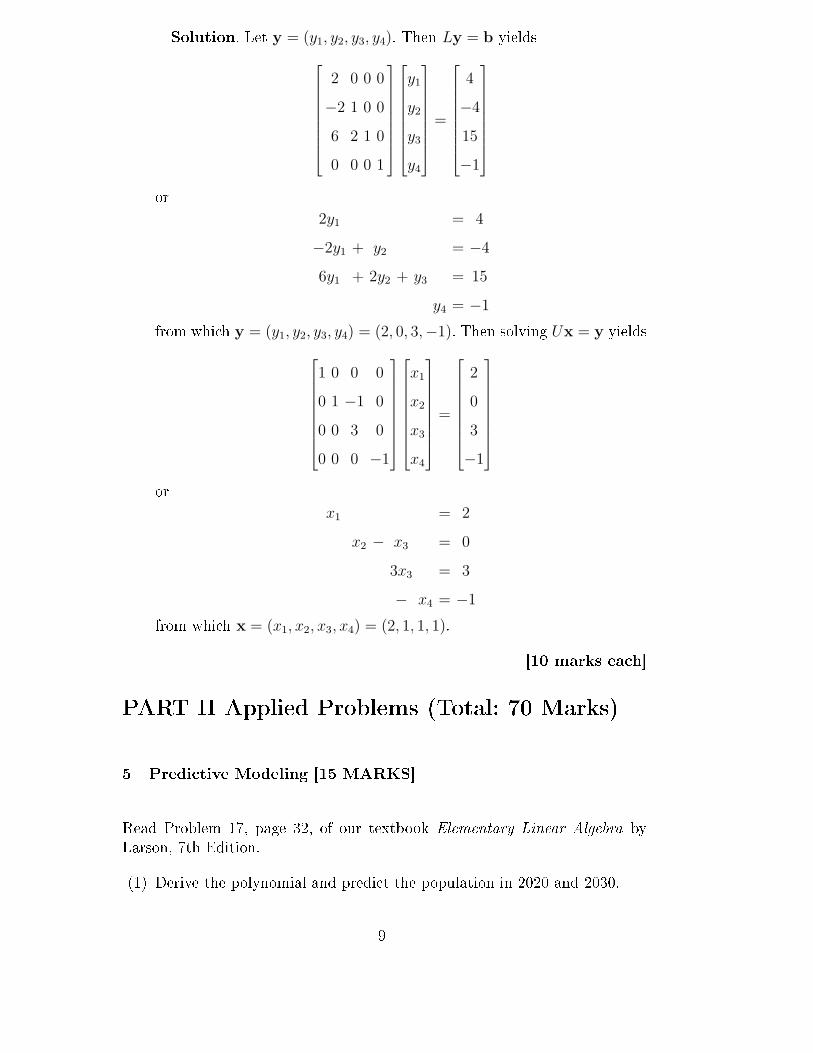
Solution. Let y = (y1, y2, y3, y4). Then Ly = b yields

2 0 0 0

−2 1 0 0

6 2 1 0

0 0 0 1

y1

y2

y3

y4

=

4

−4

15

−1

or2y1 = 4

−2y1 + y2 = −4

6y1 + 2y2 + y3 = 15

y4 = −1from which y = (y1, y2, y3, y4) = (2, 0, 3,−1). Then solving Ux = y yields

1 0 0 0

0 1 −1 0

0 0 3 0

0 0 0 −1

x1

x2

x3

x4

=

2

0

3

−1

orx1 = 2

x2 − x3 = 0

3x3 = 3

− x4 = −1from which x = (x1, x2, x3, x4) = (2, 1, 1, 1). [10 marks each]PART II Applied Problems (Total: 70 Marks)5 Predictive Modeling [15 MARKS]Read Problem 17, page 32, of our textbook Elementary Linear Algebra byLarson, 7th Edition.(1) Derive the polynomial and predict the population in 2020 and 2030.9

Solution. Let Year 0 be 1990. Then Year 10 is 2000, Year 20 is 2010,Year 30 is 2020 and Year 40 is 2030. We want to �t the polynomialp = a0 + a1t + a2t

2, t ≥ 0where t is in years, and p is in millions, through the points,(t, p) = (0, 249), (10, 281), (20, 309)Thus, we have a system of linear equations

a0 = 249

a0 + 10a1 + 100a2 = 281

a0 + 20a1 + 400a2 = 309or, since a0 = 249, we have simply10a1 + 100a2 = 281− 249 = 32

20a1 + 400a2 = 309− 249 = 60This is simple to solve to get (a1, a2) = (17/5,−1/50). Thus, the polyno-mial isp(t) = 249 +

17

5t−

1

50t2, t ≥ 0Thus, in 2020, that is, after t = 30 years, the population will be p(30) =

333 million, and in 2030, that is, after t = 40years, p(40) = 353 million.(2) Use Mathematica to plot the polynomial and extend it to include theyears up to 2030.

0 10 20 30 40t0

100

200

300

400p

Here t = 0, 10, 20, 30, 40 represent 1990, 2000, 2010, 2020 and 2030, respec-tively. [10 + 5 = 15] marks10

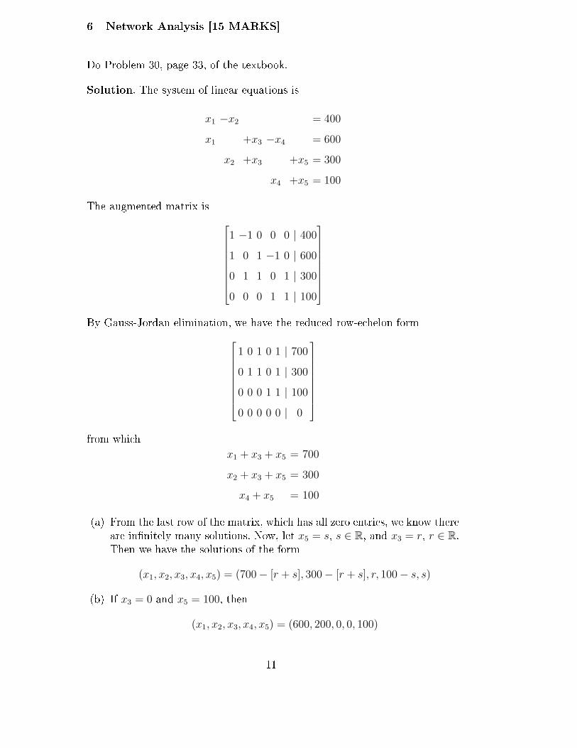
6 Network Analysis [15 MARKS]Do Problem 30, page 33, of the textbook.Solution. The system of linear equations isx1 −x2 = 400

x1 +x3 −x4 = 600

x2 +x3 +x5 = 300

x4 +x5 = 100The augmented matrix is

1 −1 0 0 0 | 400

1 0 1 −1 0 | 600

0 1 1 0 1 | 300

0 0 0 1 1 | 100

By Gauss-Jordan elimination, we have the reduced row-echelon form

1 0 1 0 1 | 700

0 1 1 0 1 | 300

0 0 0 1 1 | 100

0 0 0 0 0 | 0

from whichx1 + x3 + x5 = 700

x2 + x3 + x5 = 300

x4 + x5 = 100(a) From the last row of the matrix, which has all zero entries, we know thereare in�nitely many solutions. Now, let x5 = s, s ∈ R, and x3 = r, r ∈ R.Then we have the solutions of the form(x1, x2, x3, x4, x5) = (700− [r + s], 300− [r + s], r, 100− s, s)(b) If x3 = 0 and x5 = 100, then

(x1, x2, x3, x4, x5) = (600, 200, 0, 0, 100)11

(c) If x3 = 100 and x5 = 100, then(x1, x2, x3, x4, x5) = (500, 100, 100, 0, 100) [15 marks]7 Encryption [40 MARKS]Read Example 5 (page 88) and Example 6 (page 89). Repeat the same ex-amples, but use a di�erent 3× 3 invertible matrix, A. Will you get the samemessage?Solution. Any 3× 3 invertible matrix, A, will produce the same message.[20 + 20 = 40] marksEND OF ASSIGNMENT

12

Assignment 2 SolutionsPart I

Question 1A = 880, 10, -4, 1<, 81, 4, -1, 1<, 83, 2, 1, 2<, 8-2, -8, 2, -2<, 81, -6, 3, 0<<;

Ab = 880, 10, -4, 1, 1<, 81, 4, -1, 1, 2<,

83, 2, 1, 2, 5<, 8-2, -8, 2, -2, -4<, 81, -6, 3, 0, 1<<;

b = 81, 2, 5, -4, 1<;

MatrixForm@AbD

0 10 -4 1 1

1 4 -1 1 2

3 2 1 2 5

-2 -8 2 -2 -4

1 -6 3 0 1

MatrixForm@RowReduce@AbDDMatrixForm@LinearSolve@A, bDD

1 03

5

3

5

8

5

0 1 -

2

5

1

10

1

10

0 0 0 0 0

0 0 0 0 0

0 0 0 0 0

8

51

10

0

0

Question 2Ab = 881, 2, -3, 4<, 83, -1, 5, 2<, 84, 1, a^2 - 14, a + 2<<;

MatrixForm@AbD1 2 -3 4

3 -1 5 2

4 1 -14 + a2 2 + a

MatrixForm@RowReduce@AbDD

1 0 08

7-

1

4+a

0 1 010

7+

2

4+a

0 0 11

4+a

Plot3D@8HHx + 2 yL - 4L � 3, H2 - H3 x - yLL � 5, H6 - H4 x + yLL � 2<, 8x, -5, 5<, 8y, -5, 5<D

-50

5

-5

0

5

-10

0

10

Question 3 (i)

AI = 880, -2, 3, 1, 0, 0<, 83, 6, -3, 0, 1, 0<, 86, 6, 3, 0, 0, 1<<;

MatrixForm@AIDMatrixForm@RowReduce@AIDD

0 -2 3 1 0 0

3 6 -3 0 1 0

6 6 3 0 0 1

1 0 2 0 -

1

3

1

3

0 1 -

3

20

1

3-

1

6

0 0 0 12

3-

1

3

A = 880, -2, 3<, 83, 6, -3<, 86, 6, 3<<;

Inverse@AD

Inverse::sing : Matrix 880, -2, 3<, 83, 6, -3<, 86, 6, 3<< is singular. �

Inverse@880, -2, 3<, 83, 6, -3<, 86, 6, 3<<D

Question 3 (ii)AI = 881, 1, 2, 1, 0, 0<, 8-1, -2, 3, 0, 1, 0<, 83, -7, 4, 0, 0, 1<<;

MatrixForm@AIDMatrixForm@RowReduce@AIDD

1 1 2 1 0 0

-1 -2 3 0 1 0

3 -7 4 0 0 1

1 0 01

4-

9

26

7

52

0 1 01

4-

1

26-

5

52

0 0 11

4

5

26-

1

52

2 ASS_02_PART_I.nb

A = 881, 1, 2<, 8-1, -2, 3<, 83, -7, 4<<;

MatrixForm@Inverse@ADD1

4-

9

26

7

521

4-

1

26-

5

521

4

5

26-

1

52

Question 4A = 882, 0, 0, 0<, 8-2, 1, -1, 0<, 86, 2, 1, 0<, 80, 0, 0, -1<<;

b = 84, -4, 15, -1<;

MatrixForm@ADMatrixForm@bD

2 0 0 0

-2 1 -1 0

6 2 1 0

0 0 0 -1

4

-4

15

-1

E1 = 881 � 2, 0, 0, 0<, 80, 1, 0, 0<, 80, 0, 1, 0<, 80, 0, 0, 1<<;

A1 = E1.A;

MatrixForm@A1D1 0 0 0

-2 1 -1 0

6 2 1 0

0 0 0 -1

E2 = 881, 0, 0, 0<, 82, 1, 0, 0<, 80, 0, 1, 0<, 80, 0, 0, 1<<;

A2 = E2.E1.A;


0 1 -1 0

6 2 1 0

0 0 0 -1

E3 = 881, 0, 0, 0<, 80, 1, 0, 0<, 8-6, 0, 1, 0<, 80, 0, 0, 1<<;

A3 = E3.E2.E1.A;


0 1 -1 0

0 2 1 0

0 0 0 -1

ASS_02_PART_I.nb 3

E4 = 881, 0, 0, 0<, 80, 1, 0, 0<, 80, -2, 1, 0<, 80, 0, 0, 1<<;

A4 = E4.E3.E2.E1.A;


0 1 -1 0

0 0 3 0

0 0 0 -1

E5 = 881, 0, 0, 0<, 80, 1, 0, 0<, 80, 0, 1 � 3, 0<, 80, 0, 0, 1<<;

A5 = E5.E4.E3.E2.E1.A;


0 1 -1 0

0 0 1 0

0 0 0 -1

E6 = 881, 0, 0, 0<, 80, 1, 0, 0<, 80, 0, 1, 0<, 80, 0, 0, -1<<;

A6 = E6.E5.E4.E3.E2.E1.A;


0 1 -1 0

0 0 1 0

0 0 0 1

E7 = 881, 0, 0, 0<, 80, 1, 1, 0<, 80, 0, 1, 0<, 80, 0, 0, 1<<;

A7 = E7.E6.E5.E4.E3.E2.E1.A;


0 1 0 0

0 0 1 0

0 0 0 1

MatrixForm@[email protected]@E2D.

[email protected]@[email protected]@E6D.Inverse@E7DD2 0 0 0

-2 1 -1 0

6 2 1 0

0 0 0 -1

[email protected]

20 0 0

-

2

3

1

3

1

30

-

5

3-

2

3

1

30

0 0 0 -1

MatrixForm@Inverse@ADD1

20 0 0

-

2

3

1

3

1

30

-

5

3-

2

3

1

30

0 0 0 -1

4 ASS_02_PART_I.nb

MatrixForm@[email protected]

2

1

1

1

MatrixForm@LinearSolve@A, bDD

2

1

1

1

LU Factorization of A

L = [email protected]@[email protected]@E4D;

MatrixForm@LD2 0 0 0

-2 1 0 0

6 2 1 0

0 0 0 1

[email protected]

2 0 0 0

-2 1 -1 0

6 2 1 0

0 0 0 -1

y = 8y1, y2, y3, y4<;

[email protected] y1

-2 y1 + y2

6 y1 + 2 y2 + y3

y4

MatrixForm@bD

4

-4

15

-1

ysol = LinearSolve@L, bD

82, 0, 3, -1<

x = 8x1, x2, x3, x4<;

[email protected]

x2 - x3

3 x3

-x4

xsol = LinearSolve@A4, ysolD

82, 1, 1, 1<

ASS_02_PART_I.nb 5

Assignment 2 SolutionsPart II

Question 5A = 8810, 100<, 820, 400<<;

b = 832, 60<;

LinearSolve@A, bD

:17

5, -

1

50>

p@t_D := 249 +

17

5t -

1

50t2 ;

p@30Dp@40D333

353

Plot@p@tD, 8t, 0, 40<, LabelStyle ® Directive@LargeD,

PlotRange ® 880, 41<, 80, 400<<, GridLines ® Automatic, AxesLabel ® 8"t", "p"<D

0 10 20 30 40t0

100

200

300

400p

Question 6A = 881, -1, 0, 0, 0<, 81, 0, 1, -1, 0<, 80, 1, 1, 0, 1<, 80, 0, 0, 1, 1<<;

b = 8400, 600, 300, 100<;

Ab = 881, -1, 0, 0, 0, 400<,

81, 0, 1, -1, 0, 600<, 80, 1, 1, 0, 1, 300<, 80, 0, 0, 1, 1, 100<<;

MatrixForm@ADMatrixForm@bDMatrixForm@AbD1 -1 0 0 0

1 0 1 -1 0

0 1 1 0 1

0 0 0 1 1

400

600

300

100

1 -1 0 0 0 400

1 0 1 -1 0 600

0 1 1 0 1 300

0 0 0 1 1 100

MatrixForm@RowReduce@AbDD

1 0 1 0 1 700

0 1 1 0 1 300

0 0 0 1 1 100

0 0 0 0 0 0

TeXForm@%D

\left(\begin{array}{cccccc} 1 & 0 & 1 & 0 & 1 & 700 \\ 0 & 1 & 1 & 0 & 1 & 300 \\ 0 & 0 & 0 & 1 & 1 & 100 \\ 0 & 0 & 0 & 0 & 0 & 0 \\\end{array}\right)

LinearSolve@A, bD

8700, 300, 0, 100, 0<

2 ASS_02_PART_II.nb

Documents

Solution Assignment 2