Space-time multigrid method for molecular

dynamics simulations

Haim Waisman and Jacob Fish

Department of Civil, Mechanical and Aerospace Engineering, RensselaerPolytechnic Institute, Troy, NY 12180-3590

Abstract

We present a novel multiscale approach for molecular dynamics simulations. It isaimed at bridging discrete scales with either coarse grained discrete or continuumscales. The method consists of the waveform relaxation scheme aimed at capturingthe high frequency response of atomistic vibrations and the coarse scale solution inspace and time aimed at resolving smooth features (in both space and time domains)of the discrete medium. The method is implicit in space and time, possesses superiorstability properties and consequently enables larger time steps governed by theaccuracy considerations of coarse scale quantities of interest. Performance studieson polymer melts have shown significant speed-up compared to the classical explicitmethods, in particular on parallel machines.

Key words: Waveform relaxation, Space-Time Multigrid, Molecular Dynamicsintegration

1 Introduction

Molecular dynamics (MD) simulations provide the methodology for detailedfine scale modeling on the molecular level. MD can be viewed as a processby which one generates atomic trajectories of a system of particles by directnumerical integration of Newton’s equations of motion with the appropriateinitial and boundary conditions. The system can be formulated either by dy-namic equilibrium consideration or by means of variational principle and is

∗ Corresponding author: fishj@rpi.edu (Jacob Fish)

Preprint submitted to Elsevier Science 11 September 2005

written as

Md = F int (d)− F ext (d)

d(0) = d0

d(0) = v0

(1)

where d is a vector of atom positions, M the mass matrix and F int = −∇Φ(d)the force field defined as the gradient of the potential energy.Current MD algorithms severely restrict the modeling efforts to relativelysmall systems and/or short time intervals. The algorithmic challenges fac-ing MD simulations stem from the difficulty of designing methods which areinsensitive in terms of the integration time step to rapid fluctuations in chem-ical bonds and short ranged forces. Most widely used algorithms in MD areexplicit methods, such as Verlet and Gear’s predictor-corrector methods. Asevere limitation in the ability of the explicit methods to propagate numericaltrajectories stems from a wide range of time scales spanning many orders ofmagnitude. For instance, in polymer chains, bond-stretching vibrations arethe fastest atomic motions in a molecule, typically in the order of femtosec-onds, whereas the relaxation of polymers in the form of segmental motions orterminal relaxations of chains is spanning the time scales in the range between10−2s to 104s The maximum time step is limited by the smallest oscillationperiod that can be found in the simulated system. This time step is necessaryto maintain stability of explicit numerical integration schemes [1].Considerable efforts have been devoted to increasing the critical time step.Many insightful observations on the numerical properties of the algorithmswere reported, and numerous improvements have been proposed. Neverthe-less, the increases in the integration time step have been quite modest sofar [2]. This temporal gap can be partially circumvented by parallel algorithms.However, due to inherently sequential nature of time integration schemes, par-allelism has been exploited in the spatial domain only, while computations intime domain remain primarily sequential. One promising research avenue isto develop integration algorithms, which are parallelizable in time domain. Adifferent (or complimentary) approach is to exploit implicit integration. Im-plicit methods require solution of coupled nonlinear equations at every timestep, which is both expensive and difficult to implement. Nevertheless, theyreduce stability restrictions and enable much larger time step, typically gov-erned by accuracy considerations [3, 4]. In general, accuracy means how closeis the solution of atomic trajectories obtained by the numerical integrationto the true trajectories. We refer to this type of definition as the accuracy inlocal quantities. Molecular systems, however, are highly nonlinear and exhibitsensitive dependence on perturbations. Moreover, the initial conditions areusually assigned randomly. Thus, accurate approximation of local trajectorieson meaningful time intervals is neither obtainable nor desired. This suggeststo analyzing the accuracy with respect to the global quantities of interest,such as temperature, energy, diffusion and others.In the present manuscript we present a novel multiscale approach based on

2

the space-time variational multigrid principle for molecular systems charac-terized by diverse spatial and temporal scales. Our approach is implicit inboth space and time domains that uses typically 10 to 50 times larger timesteps than explicit methods selected based on the accuracy of global fields ofinterest. The space-time character of the method provides an improved stabil-ity without directly solving the space-time problem. The multiscale nature ofthe system is exploited in two ways: First, it substantially reduces the cost ofmultigrid iterations (see Section 2.1), and secondly, it is parallelizable in timedomain by exploiting the waveform relaxation (WR) scheme in the smoothingprocess (see Section 2.2). In Section 3 we develop the variational space-timemultigrid method suitable for MD simulations, which exploits the multiscalenature of the problem. It consists of the WR scheme aimed at capturing theresponse atomistic vibrations and the coarse scale solution in space and timeintended to resolve the slow features of the discrete medium. The coarse gridproblem is derived from the Hamilton’s principle on the subspace of coarsescale functions. In Section 4 we show that for linear case the method reducesto the sequential multigrid method [5]. Performance studies are conducted inSection 5.

2 Motivation

2.1 Multigrid as a multiscale solver

The motivation for use of multigrid ideas for multiscale problems was givenin [6, 7]. To convey the basic ideas, consider a continuum one-dimensionaltwo-scale elliptic problem for the scalar field u

ddx

(k(x)du

dx

)+ b(x) = 0

u(0) = u(L) = 0(2)

on the interval x ∈ [0, L] with oscillatory periodic piecewise constant coeffi-cients k1 and k2 and 0.5 volume fraction. In many applications of interest andin particular those described at the atomistic scale k1 À k2 yielding highlyheterogenous systems. Equation (2) is discretized using finite elements or fi-nite difference leading to a linear system Ku = f . Analyzing the eigenvaluesof K reveals the following. The eigenvalues are clustered at the two ends of thespectrum on the right half plane. More importantly, the eigenvalues clusteredclose to zero are identical to those obtained by the problem with homogenizedcoefficients [6, 7]. This character of the spectrum suggests a computationalstrategy based on the philosophy of multigrid methods. In such a multigridstrategy the smoother is designed to capture the higher frequency response ofthe fine scale model represented by a linear combination of the highest eigen-

3

modes. The auxiliary coarse model is then engineered to effectively capturethe remaining lower frequency response of the fine scale problem. For a pe-riodic heterogeneous medium, such an auxiliary coarse model coincides withthe boundary value problem with homogenized coefficients as evidenced by theidentical eigenvalues. The resulting multiscale prolongation operator is givenby

Q = Qc + Qf

where Qc and Qf are the classical (smooth) prolongation and the fine scalecorrection obtained from the discretization of the influence functions, respec-tively. The rate of convergence of the multigrid process for the two-scale prob-lem given by Eq. (2) is governed by [6, 7]

‖ei+1‖ =q

4− q‖ei‖

where ‖ei+1‖ is the norm of the error at iteration i + 1 and

q =2√

k1k2

(k1 + k2). (3)

Note that for k1 = k2 the media is homogeneous, and one recovers the clas-sical multigrid rate of 1

3[8]. However, for example if either k1

k2or k2

k1is 100,

then the convergence factor reduces to 15

and the two-scale process convergesin five iterations up to the tolerance of 10−5. In this manuscript we devisea multilevel-like strategy for efficient solution of MD equations. We view theintegration of Newton’s equations of motion as problem on a space-time grid.This observation suggests a unique space-time multigrid approach that ex-ploits multiple spatial and temporal scales of a molecular system.

2.2 The waveform relaxation scheme

One of the major barriers for efficient solution of large scale MD equations isthe sequential character of time integration methods. The waveform relaxation(WR) method is an iterative solution of space-time problems that offers par-allelization [9, 10]. Due to its implicit nature, WR provides superior stabilityand large time steps compared to explicit methods.In the WR algorithm, the space-time domain is partitioned in space intosmaller subsystems, thereafter to be referred to as the spatial blocks or sim-ply blocks. Each block is then integrated over the temporal grid. The spatialblocks can be integrated independently on different processors. The temporalgrid is divided into intervals called windows. Windows are used to accelerateconvergence and to reduce storage. At every time step an algebraic system ofequations is solved on a spatial grid. See Figure 1 for definitions. Informationtransfer between different windows takes place once the integration over the

4

Time

Spatial Slab

Spatial Block

Window

t∆

Space (1D)

Temporal grid

Atoms

Fig. 1. Slabs, windows and blocks in the waveform relaxation method

corresponding windows is completed. The main advantage of the method isthat it permits simultaneous integration of spatial blocks in each window andits ability for unstructured integration. For instance, spatial blocks involvingstiff connections will require smaller time steps than those having more com-pliant connections analogous to the multiple time step (MTS) techniques [2].The WR method has been primarily used in electrical network simulationsand parabolic initial value problems. Limited studies have been conductedfor hyperbolic [11] and second order [12] systems. In the remaining of thissection we give some technical details of the WR method focusing on non-linear systems. For highly nonlinear systems, such as those arising from MDsimulations, two versions of WR method are common. The first is a direct ex-tension of the linear WR formulations, so called Waveform Relaxation Newton(WRN) method [13]. In the MD context, the basic idea is to solve the followingnonlinear scalar equations

midν+1i = F int(dν

1, ..., dνi−1, d

ν+1i , dν

i+1, ..., dνN)

dν+1i (0) = d0i

dν+1i (0) = v0i

(4)

for every atom i in the system (without lost of generality, we assume F ext = 0).The superscripts, ν and ν+1 , denote the iteration count within a time windowt ∈ [t0, tn].Each atom (or a spatial block consisting of several atoms) in iteration ν + 1is integrated over a time window based on its previous position in time (inthe same iteration ν + 1) and the information about its neighbor positions.As opposed to classical integrators, neighboring positions are taken from the

5

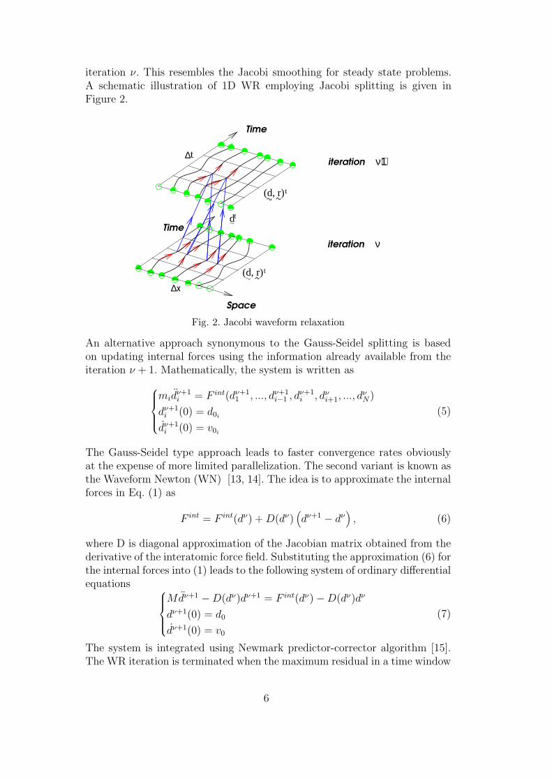
iteration ν. This resembles the Jacobi smoothing for steady state problems.A schematic illustration of 1D WR employing Jacobi splitting is given inFigure 2.

Time

td

Time

νiteration

ν+1iteration

Space

� �� �� ��������� �� �� ����

� �� �� ���� � �� �� � ���� �� �� � � �� �� ���� �� ���� �� �� ��� t(d, r)

t(d, r)

x∆

t∆

� �� �� ���

� �� �� ����� �� �� ���� �� �� ����� �� ���� �� �� ���� !!" "" "" "###

$$%%& && &'' ( (( (( ())* ** ** *+++, ,, ,--. .. .. .// 0 00 011

2 22 22 23334 44 44 45556 66 66 677

Fig. 2. Jacobi waveform relaxation

An alternative approach synonymous to the Gauss-Seidel splitting is basedon updating internal forces using the information already available from theiteration ν + 1. Mathematically, the system is written as

midν+1i = F int(dν+1

1 , ..., dν+1i−1 , dν+1

i , dνi+1, ..., d

νN)

dν+1i (0) = d0i

dν+1i (0) = v0i

(5)

The Gauss-Seidel type approach leads to faster convergence rates obviouslyat the expense of more limited parallelization. The second variant is known asthe Waveform Newton (WN) [13, 14]. The idea is to approximate the internalforces in Eq. (1) as

F int = F int(dν) + D(dν)(dν+1 − dν

), (6)

where D is diagonal approximation of the Jacobian matrix obtained from thederivative of the interatomic force field. Substituting the approximation (6) forthe internal forces into (1) leads to the following system of ordinary differentialequations

Mdν+1 −D(dν)dν+1 = F int(dν)−D(dν)dν

dν+1(0) = d0

dν+1(0) = v0

(7)

The system is integrated using Newmark predictor-corrector algorithm [15].The WR iteration is terminated when the maximum residual in a time window

6

is smaller than a specified tolerance

max{‖rν+1(t)‖2} = max{‖Mdν+1 − F int(dν+1

1 , ..., dν+1i , ..., dν+1

N

)‖}. (8)

or alternatively when

max{‖dν+1(t)− dν(t)‖} ≤ ε, (9)

for some small positive constant ε. The major drawback of the WR method(both aforementioned versions) is in its slow convergence in case of a strongcoupling between spatial blocks and sizable windows [16, 17]. In the proposedvariational space-time multigrid approach (presented in Section 3) the WRtakes the role of smoother aimed at capturing the high frequency response ofatomistic vibrations. To this end we note that the combination of the WRsmoothing and the coarse grid correction is not new. The so-called multigridwaveform relaxation (MWR) has been developed in [18, 19] in the context ofparabolic partial differential equations. However, for highly nonlinear molec-ular dynamics systems we find this approach either slow to converge or notconverging at all.

3 Variational space-time multigrid method

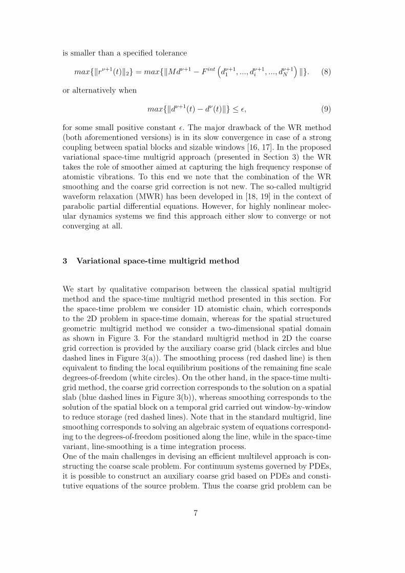
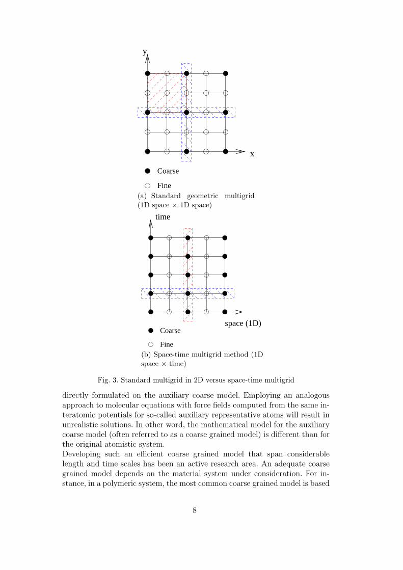
We start by qualitative comparison between the classical spatial multigridmethod and the space-time multigrid method presented in this section. Forthe space-time problem we consider 1D atomistic chain, which correspondsto the 2D problem in space-time domain, whereas for the spatial structuredgeometric multigrid method we consider a two-dimensional spatial domainas shown in Figure 3. For the standard multigrid method in 2D the coarsegrid correction is provided by the auxiliary coarse grid (black circles and bluedashed lines in Figure 3(a)). The smoothing process (red dashed line) is thenequivalent to finding the local equilibrium positions of the remaining fine scaledegrees-of-freedom (white circles). On the other hand, in the space-time multi-grid method, the coarse grid correction corresponds to the solution on a spatialslab (blue dashed lines in Figure 3(b)), whereas smoothing corresponds to thesolution of the spatial block on a temporal grid carried out window-by-windowto reduce storage (red dashed lines). Note that in the standard multigrid, linesmoothing corresponds to solving an algebraic system of equations correspond-ing to the degrees-of-freedom positioned along the line, while in the space-timevariant, line-smoothing is a time integration process.One of the main challenges in devising an efficient multilevel approach is con-structing the coarse scale problem. For continuum systems governed by PDEs,it is possible to construct an auxiliary coarse grid based on PDEs and consti-tutive equations of the source problem. Thus the coarse grid problem can be

7

Fine

Coarse

x

y

(a) Standard geometric multigrid(1D space × 1D space)

time

space (1D)

Fine

Coarse

(b) Space-time multigrid method (1Dspace × time)

Fig. 3. Standard multigrid in 2D versus space-time multigrid

directly formulated on the auxiliary coarse model. Employing an analogousapproach to molecular equations with force fields computed from the same in-teratomic potentials for so-called auxiliary representative atoms will result inunrealistic solutions. In other word, the mathematical model for the auxiliarycoarse model (often referred to as a coarse grained model) is different than forthe original atomistic system.Developing such an efficient coarse grained model that span considerablelength and time scales has been an active research area. An adequate coarsegrained model depends on the material system under consideration. For in-stance, in a polymeric system, the most common coarse grained model is based

8

on the equation of motion of the Langevin type (also known as Brownian dy-namics)

M∂2Ri

∂2t+ C

∂Ri

∂t= F s

i

where Ri is the position of coarse grained particle i (or blob) M is its mass;C the equivalent friction between polymer chains; and F s

i represents both theGaussian random forces and the force, which mimic molecular collisions andtherefore a thermal reservoir (see for example [20, 21]). In the present man-uscript we adopt a different approach by which the coarse grained equationsare constructed directly from the fine scale using Hamilton’s principle on thesubspace of the coarse scale functions. The proposed formulation providesa superior rate of convergence, but is computationally more expensive thanevolving the coarse grained model directly since it involves computations ofthe force fields on the fine scale. Let e be the coarse scale correction aimedat updating the fine scale solution, where m ¿ N is the size of the coarsemodel. The updated fine scale solution at a certain time step is given bydν+1 ← dν +Qe where dν ∈ RN . To find the optimal correction we express theLagrangian in terms of the correction Qe

L(Qe,Qe) =1

2< M(dν + Qe), (dν + Qe) > −Φ(dν + Qe). (10)

The prolongation Q is assumed to be constant over a certain period of time.By Hamilton’s principle e(t) is the minimizer of

S[e(t)] =∫ t2

t1L(Qe,Qe)dt, (11)

written asδS

δe(t)= 0 t1 < t < t2. (12)

which is equivalent to solving the following Euler-Lagrange equations

d

dt

(∂L

∂e

)− ∂L

∂e=

δS

δe(t)= 0. (13)

Substituting the Lagrangian into (13) results in the following coarse grid prob-lem

QT MQe−QT F int(dν + Qe) = −QT Mdν

e(0) = 0

e(0) = 0

(14)

We will refer to Eq. (14) as the coarse grid correction in space and time.The system (14) can be integrated explicitly or implicitly. For the latter, ourexperience indicates (see Section 5) that it is sufficient to perform only oneor two Newton iterations to reduce the computational cost. Once the erroris calculated it is prolongated to the fine scale at each time step within a

9

window. Algorithmic details of the nonlinear space-time multigrid method aresummarized in tables corresponding to Algorithms 1, 2 and 3. Capital lettersindicate matrices and capital letters with subscript t indicate a column ina matrix corresponding to discrete time t. An illustration of the space-timemultigrid method is presented in Figure 4. Arrows depicts the informationflow.

Time

t

dt

Q rtT

coarse grid evolution

Space

Time

Timee

Qe

t

Space

� �� �� ��� � �� �� ���� �� �� ����

� �� �� ���� �� �� ���� �� �� � � �� �� ����� �� ���

� �� �� ���� �� �� ���� �� ��� � �� �� ���� �� �� ��� � �� �� ����

� �� �� ����∆x

∆t

(d, r)t

iteration ν+1

iteration ν !!" "" "##$ $$ $$ $%%

& && && &''

( (( ())

* ** ** *+++ , ,, ,, ,--

. .. .. .// 0 00 0112 22 22 233 4 44 44 455 6 66 66 6778 88 88 899 : :: :: :;;;

< << <==> >> >> >??? @ @@ @@ @AAB BB BB BCCCD DD DD DEE F FF FF FGGG

Fig. 4. Space-Time multigrid method

Algorithm 1 Nonlinear space-time multigrid method

1: [M, d0, v0, t0, tn] = setup()2: X ← [d1, .., dn] {%} initialize on space-time3: while normR ≥ tol do4: X0 = X5: [X,A] = WRNL(M, X, d0, v0, t0, tn, ν1) {%} smooth ν1 times6: X = MG(M, X,A, t0, tn) {%} coarse grid evolution7: [X,A] = WRNL(M, X, d0, v0, t0, tn, ν2) {%} smooth ν2 times8: normR ← max{‖Xt −X0

t ‖2} {%} compute residual9: end while

Remark 1: In the case of Harmonic potentials, i.e. F int(d) = −Kd the coarsegrid correction in space and time is consistent with the linear formulationsgiven in [18]

QT MQe + QT KQe = QT rs

e(0) = 0

e(0) = 0

(15)

where rs = −Kdν+1s − Mdν+1

s is the defect computed on the fine scale aftersmoothing.Remark 2: The performance of the variational space-time multigrid methodcan be improved using the windowing technique. By this approach the integra-tion domain is broken into non-overlapping subintervals [0, T1], [T1, T2], ..., [Tn−1, Tn]

10

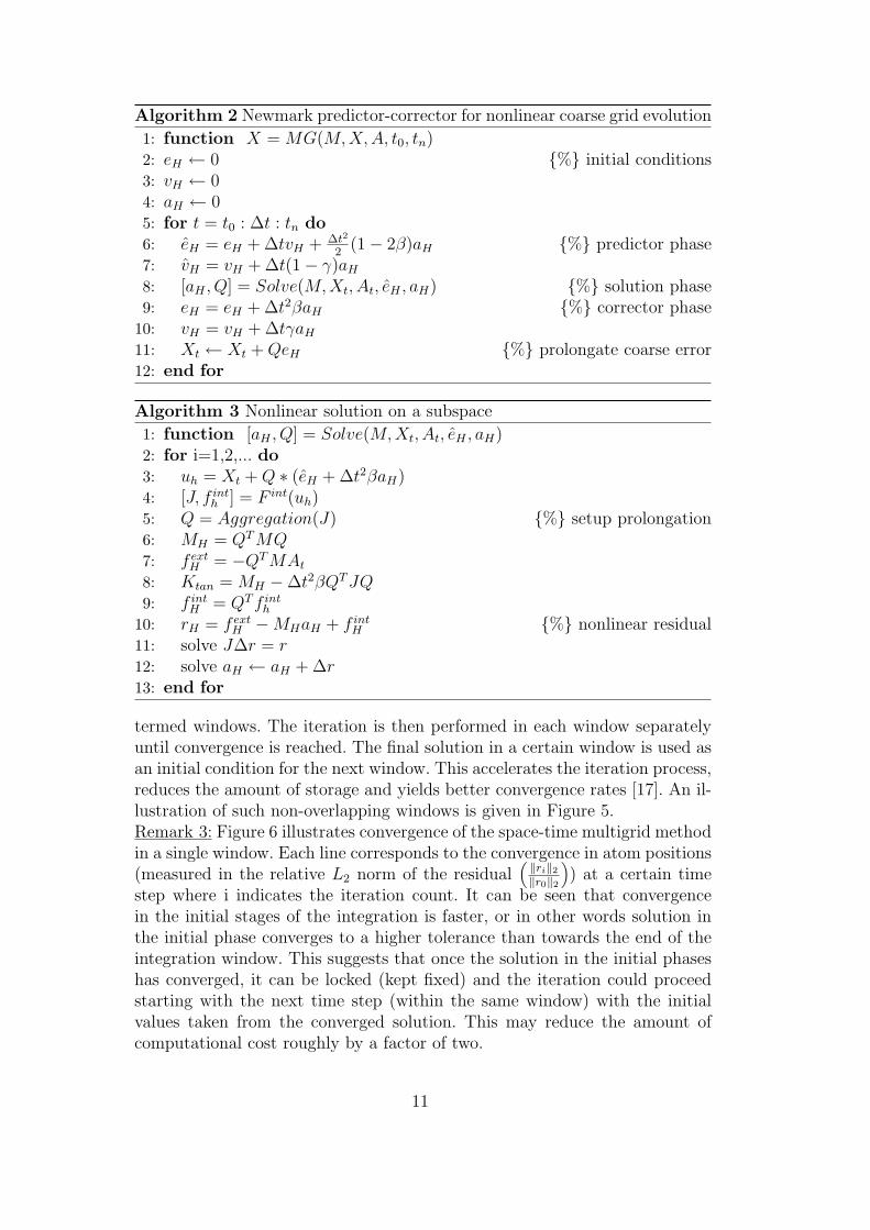
Algorithm 2 Newmark predictor-corrector for nonlinear coarse grid evolution

1: function X = MG(M, X,A, t0, tn)2: eH ← 0 {%} initial conditions3: vH ← 04: aH ← 05: for t = t0 : ∆t : tn do6: eH = eH + ∆tvH + ∆t2

2(1− 2β)aH {%} predictor phase

7: vH = vH + ∆t(1− γ)aH

8: [aH , Q] = Solve(M,Xt, At, eH , aH) {%} solution phase9: eH = eH + ∆t2βaH {%} corrector phase

10: vH = vH + ∆tγaH

11: Xt ← Xt + QeH {%} prolongate coarse error12: end for

Algorithm 3 Nonlinear solution on a subspace

1: function [aH , Q] = Solve(M,Xt, At, eH , aH)2: for i=1,2,... do3: uh = Xt + Q ∗ (eH + ∆t2βaH)4: [J, f int

h ] = F int(uh)5: Q = Aggregation(J) {%} setup prolongation6: MH = QT MQ7: f ext

H = −QT MAt

8: Ktan = MH −∆t2βQT JQ9: f int

H = QT f inth

10: rH = f extH −MHaH + f int

H {%} nonlinear residual11: solve J∆r = r12: solve aH ← aH + ∆r13: end for

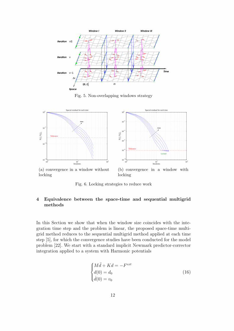
termed windows. The iteration is then performed in each window separatelyuntil convergence is reached. The final solution in a certain window is used asan initial condition for the next window. This accelerates the iteration process,reduces the amount of storage and yields better convergence rates [17]. An il-lustration of such non-overlapping windows is given in Figure 5.Remark 3: Figure 6 illustrates convergence of the space-time multigrid methodin a single window. Each line corresponds to the convergence in atom positions(measured in the relative L2 norm of the residual

( ‖ri‖2‖r0‖2

)) at a certain time

step where i indicates the iteration count. It can be seen that convergencein the initial stages of the integration is faster, or in other words solution inthe initial phase converges to a higher tolerance than towards the end of theintegration window. This suggests that once the solution in the initial phaseshas converged, it can be locked (kept fixed) and the iteration could proceedstarting with the next time step (within the same window) with the initialvalues taken from the converged solution. This may reduce the amount ofcomputational cost roughly by a factor of two.

11

Window II Window III

Space

Time

Window I

(d, r)tI

����������

��������������

��� �� �

�����

�����������������

����������

�����������������

!!"""###$$$%%%

&&&'''

((())

* ** *++,,,--

..//00011

222333444555

66677

νiteration

iteration ν−1

iteration ν+1

∆x

∆t

888999: :: :;;

<<<===

>>>??

@ @@ @AABBBCCC

DDDEE

FFFGGHHHII JJJKKK

LLLMMMNNNOO PPPQQ

RRRSSTTTUUU

VVVWW XXXYYYZZZ[[

\\\]]

^^__

``aa

bbccddeeffgghhii

jjkkllmm

nnooppqqrrssttuuvvwwxxyy

zzz{{{

||}}

~~�� ��������

���������

���� ���������

����

Fig. 5. Non-overlapping windows strategy

100

101

102

10−15

10−10

10−5

100

Spacial residual for each time

Iterations

||ri|| 2/ |

|r 0|| 2

Tolerance

time

(a) convergence in a window withoutlocking

100

101

102

10−10

10−8

10−6

10−4

10−2

100

Spacial residual for each time

Iterations

||ri|| 2/ |

|r 0|| 2

Tolerance

time

Locked

(b) convergence in a window withlocking

Fig. 6. Locking strategies to reduce work

4 Equivalence between the space-time and sequential multigridmethods

In this Section we show that when the window size coincides with the inte-gration time step and the problem is linear, the proposed space-time multi-grid method reduces to the sequential multigrid method applied at each timestep [5], for which the convergence studies have been conducted for the modelproblem [22]. We start with a standard implicit Newmark predictor-correctorintegration applied to a system with Harmonic potentials

Md + Kd = −F ext

d(0) = d0

d(0) = v0

(16)

12

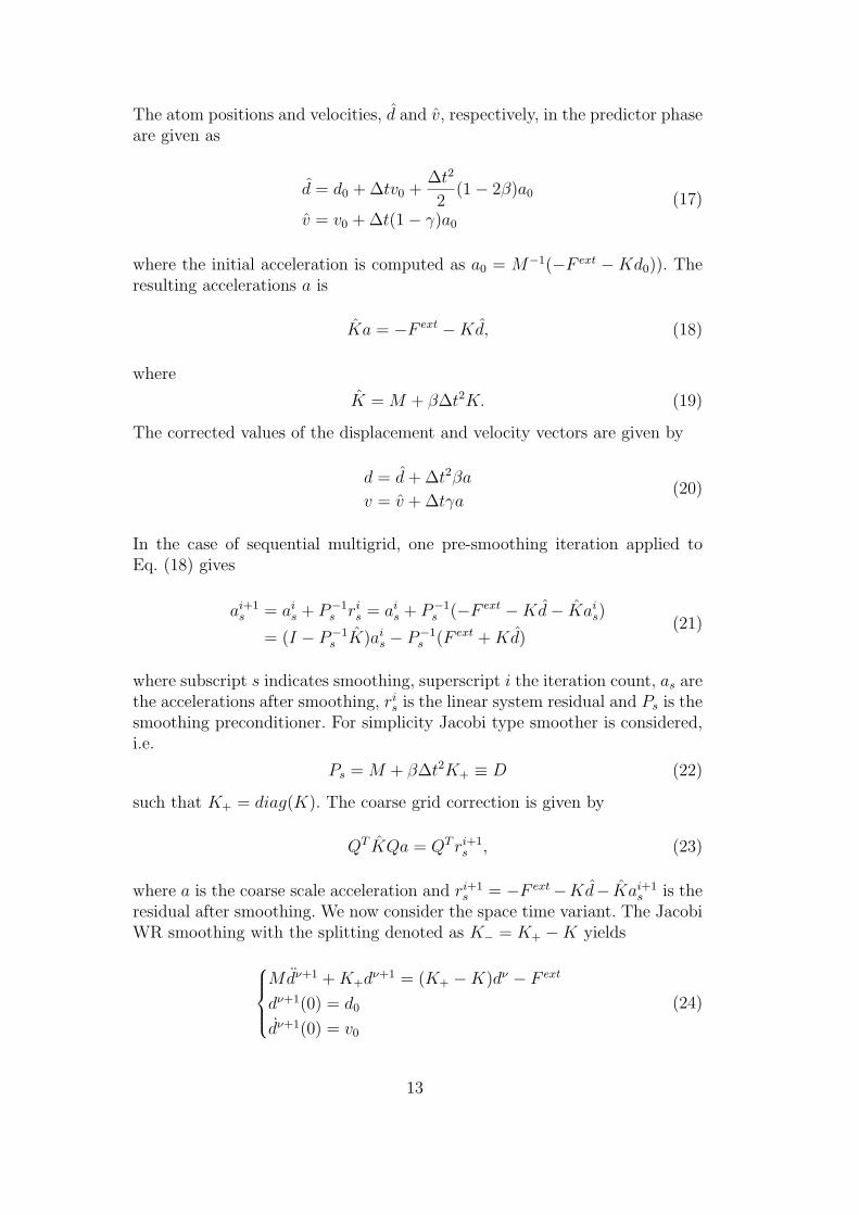
The atom positions and velocities, d and v, respectively, in the predictor phaseare given as

d = d0 + ∆tv0 +∆t2

2(1− 2β)a0

v = v0 + ∆t(1− γ)a0

(17)

where the initial acceleration is computed as a0 = M−1(−F ext −Kd0)). Theresulting accelerations a is

Ka = −F ext −Kd, (18)

where

K = M + β∆t2K. (19)

The corrected values of the displacement and velocity vectors are given by

d = d + ∆t2βa

v = v + ∆tγa(20)

In the case of sequential multigrid, one pre-smoothing iteration applied toEq. (18) gives

ai+1s = ai

s + P−1s ri

s = ais + P−1

s (−F ext −Kd− Kais)

= (I − P−1s K)ai

s − P−1s (F ext + Kd)

(21)

where subscript s indicates smoothing, superscript i the iteration count, as arethe accelerations after smoothing, ri

s is the linear system residual and Ps is thesmoothing preconditioner. For simplicity Jacobi type smoother is considered,i.e.

Ps = M + β∆t2K+ ≡ D (22)

such that K+ = diag(K). The coarse grid correction is given by

QT KQa = QT ri+1s , (23)

where a is the coarse scale acceleration and ri+1s = −F ext−Kd− Kai+1

s is theresidual after smoothing. We now consider the space time variant. The JacobiWR smoothing with the splitting denoted as K− = K+ −K yields

Mdν+1 + K+dν+1 = (K+ −K)dν − F ext

dν+1(0) = d0

dν+1(0) = v0

(24)

13

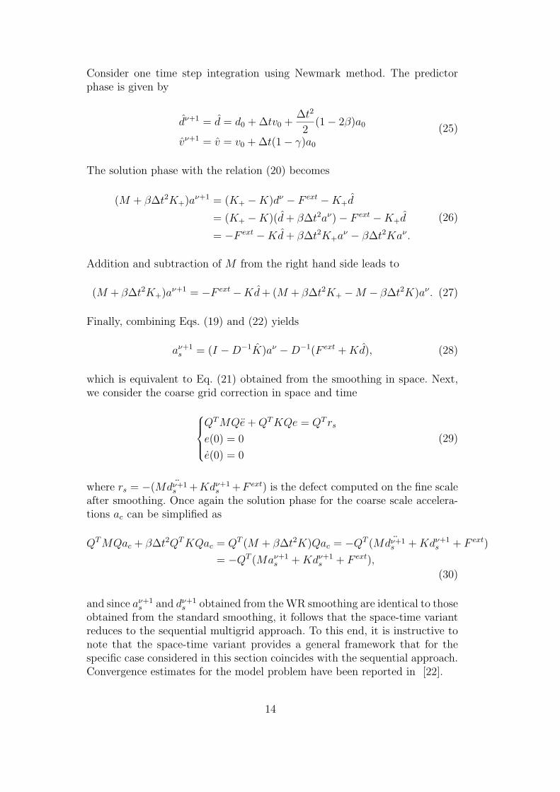
Consider one time step integration using Newmark method. The predictorphase is given by

dν+1 = d = d0 + ∆tv0 +∆t2

2(1− 2β)a0

vν+1 = v = v0 + ∆t(1− γ)a0

(25)

The solution phase with the relation (20) becomes

(M + β∆t2K+)aν+1 = (K+ −K)dν − F ext −K+d

= (K+ −K)(d + β∆t2aν)− F ext −K+d

= −F ext −Kd + β∆t2K+aν − β∆t2Kaν .

(26)

Addition and subtraction of M from the right hand side leads to

(M + β∆t2K+)aν+1 = −F ext −Kd + (M + β∆t2K+ −M − β∆t2K)aν . (27)

Finally, combining Eqs. (19) and (22) yields

aν+1s = (I −D−1K)aν −D−1(F ext + Kd), (28)

which is equivalent to Eq. (21) obtained from the smoothing in space. Next,we consider the coarse grid correction in space and time

QT MQe + QT KQe = QT rs

e(0) = 0

e(0) = 0

(29)

where rs = −(M ¨dν+1s +Kdν+1

s +F ext) is the defect computed on the fine scaleafter smoothing. Once again the solution phase for the coarse scale accelera-tions ac can be simplified as

QT MQac + β∆t2QT KQac = QT (M + β∆t2K)Qac = −QT (M ¨dν+1s + Kdν+1

s + F ext)

= −QT (Maν+1s + Kdν+1

s + F ext),

(30)

and since aν+1s and dν+1

s obtained from the WR smoothing are identical to thoseobtained from the standard smoothing, it follows that the space-time variantreduces to the sequential multigrid approach. To this end, it is instructive tonote that the space-time variant provides a general framework that for thespecific case considered in this section coincides with the sequential approach.Convergence estimates for the model problem have been reported in [22].

14

5 Numerical results

In this section we conduct performance studies of the space-time multigridmethod on a model problem of an atomistic chain and a polymer melt.

5.1 Atomistic chain with Harmonic potentials

We first consider an atomistic chain with heterogeneous Harmonic potentials inperiodic arrangement with one stiff and one compliant connection; the stiffnessratio between the two connection is taken as

kstiff

ksoft= 100. We consider periodic

long interactions such that each atom interacts with 10 closest neighbors.Newmark predictor-corrector algorithm is used to integrate the equations ofmotion. The integration time step for the explicit velocity-verlet method islimited by stability considerations. The critical step is obtained by consideringhow fast a wave travels in the stiffest cell, given by

∆tcr =2√

ρ(A),

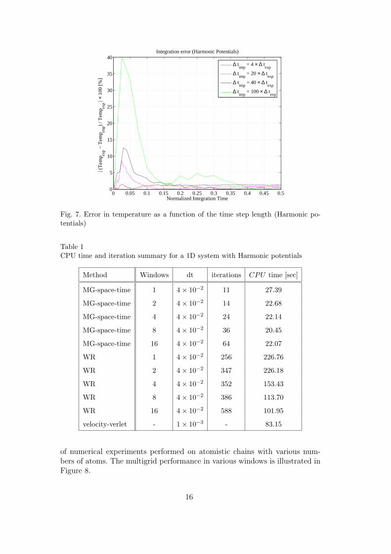
where ρ(A) is the spectral radius (highest eigenvalue) of A = M−1K [15].For the multigrid and waveform methods considered, the length of the timestep is governed by the accuracy of the coarse fields of interest, selected hereas temperature, which is the average kinetic energy of the system. Figure 7depicts the relative error in the implicit methods computed as

Er[%] =|Tempexp − Tempimp|

|Tempexp| × 100, (31)

where Tempexp is the temperature obtained by the velocity-verlet methodand Tempimp is the temperature obtained by the implicit methods for vari-ous time steps. Despite the fact that the implicit time step is 40 times largerthan that of the explicit scheme the normalized error in of the temperature, atsteady-state, is less than 0.5%. Consequently, the time step for the space-timemultigrid method is chosen as ∆timp = 40×∆texp. Table 1 reports convergenceresults for the space-time multigrid method compared to the velocity-verletand waveform relaxation method. The atomic chain consists of 1001 atomsand is integrated over 16 implicit time steps. We use one pre Jacobi smooth-ing and a coarse grid correction. The coarse grid possess homogenized materialproperties [6, 7]. Various columns in Table 1 correspond to the type of method,number of windows selected, integration time step (dt), total number of it-erations and overall CPU time. All calculations were performed on a singleprocessor machine. It can be seen that the space-time multigrid method hasthe best performance. To study the windowing strategy, we conduct a series

15

0 0.05 0.1 0.15 0.2 0.25 0.3 0.35 0.4 0.45 0.50

5

10

15

20

25

30

35

40

Normalized Integration Time

| (T

emp ex

p − T

emp im

p) / T

emp ex

p | ×

100

[%]

Integration error (Harmonic Potentials)

∆ timp

= 4 × ∆ texp

∆ timp

= 20 × ∆ texp

∆ timp

= 40 × ∆ texp

∆ timp

= 100 × ∆ texp

Fig. 7. Error in temperature as a function of the time step length (Harmonic po-tentials)

Table 1CPU time and iteration summary for a 1D system with Harmonic potentials

Method Windows dt iterations CPU time [sec]

MG-space-time 1 4× 10−2 11 27.39

MG-space-time 2 4× 10−2 14 22.68

MG-space-time 4 4× 10−2 24 22.14

MG-space-time 8 4× 10−2 36 20.45

MG-space-time 16 4× 10−2 64 22.07

WR 1 4× 10−2 256 226.76

WR 2 4× 10−2 347 226.18

WR 4 4× 10−2 352 153.43

WR 8 4× 10−2 386 113.70

WR 16 4× 10−2 588 101.95

velocity-verlet - 1× 10−3 - 83.15

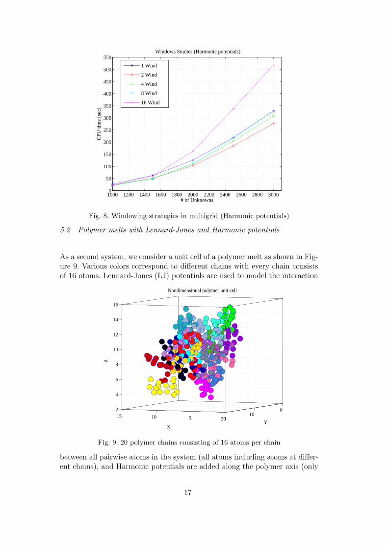
of numerical experiments performed on atomistic chains with various num-bers of atoms. The multigrid performance in various windows is illustrated inFigure 8.

16

1000 1200 1400 1600 1800 2000 2200 2400 2600 2800 30000

50

100

150

200

250

300

350

400

450

500

550

# of Unknowns

CPU

tim

e [s

ec]

Windows Studies (Harmonic potentials)

1 Wind

2 Wind

4 Wind

8 Wind

16 Wind

Fig. 8. Windowing strategies in multigrid (Harmonic potentials)

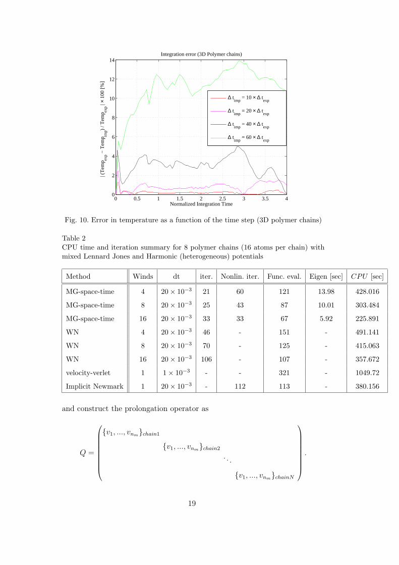
5.2 Polymer melts with Lennard-Jones and Harmonic potentials

As a second system, we consider a unit cell of a polymer melt as shown in Fig-ure 9. Various colors correspond to different chains with every chain consistsof 16 atoms. Lennard-Jones (LJ) potentials are used to model the interaction

0510150

1020

2

4

6

8

10

12

14

16

Y

Nondimensional polymer unit cell

X

zz

Fig. 9. 20 polymer chains consisting of 16 atoms per chain

between all pairwise atoms in the system (all atoms including atoms at differ-ent chains), and Harmonic potentials are added along the polymer axis (only

17

within a chain). Mathematically we have

Φ =N∑

i=1

N−1∑

j>1

ΦLJ(rij) +1

2

∑

bonds

kbondc (rc − r0)

2. (32)

The LJ potential describes the energy of interaction between two atoms as afunction of the distance between their centers rij. The standard pairwise LJpotential is given by

ΦLJ(rij) = 4ε

(σ

rij

)12

−(

σ

rij

)6 (33)

where rij =√

(rx,i − rx,j)2 + (ry,i − ry,j)2 + (rz,i − rz,j)2; ε is the well-depth ofthe interaction and σ is the collision diameter. The total potential energy isgiven as a sum over all pairs

Φ =1

2

N∑

i=1

N∑

j=1i 6=j

ΦLJ(rij) =N∑

i=1

N−1∑

j>1

ΦLJ(rij). (34)

In our simulations we use normalized units with ε = σ = 1 and heterogeneousHarmonic potentials to model the chains. That is, different bond stretchingconstants kbond

c are used for different chains. Specifically,

kbondc =

1 c = 1, 3, ...

10 c = 2, 4, ...(35)

and r0 = 1. This heterogeneity creates a range of time scales, and thus theexplicit velocity-verlet algorithm, due to stability requirement, is limited bythe fast vibrating components. As before, we control the accuracy in temper-ature. Figure 10 shows the normalized error in temperature for 20 polymerchains that consist of 16 atoms per chain (see Figure 9). We use the explicitmethod with ∆texp = 1×10−3 as the reference solution. The allowable error intemperature is selected to be 1.5%. This corresponds to the implicit time stepthat is 20 times larger than the explicit time step. The system is integratedover 16 implicit steps. We apply one presmoothing of Jacobi waveform Newton(WN). The iteration is terminated when ‖dν+1 − dν‖2 ≤ 10−4 for all times.The prolongation operator in the space-time multigrid method is computedbased on the aggregation approach [23]. Specifically, we form a local Jacobianmatrix for every aggregate Jagg. In our case each aggregate corresponds to onepolymer chain. We select the 32 lowest modes by solving the eigen problem

Jaggvi = λivi i = 1, .., nm (36)

18

0 0.5 1 1.5 2 2.5 3 3.5 40

2

4

6

8

10

12

14

Normalized Integration Time

| (T

emp ex

p − T

emp im

p) / T

emp ex

p | ×

100

[%]

Integration error (3D Polymer chains)

∆ timp

= 10 × ∆ texp

∆ timp

= 20 × ∆ texp

∆ timp

= 40 × ∆ texp

∆ timp

= 60 × ∆ texp

Fig. 10. Error in temperature as a function of the time step (3D polymer chains)

Table 2CPU time and iteration summary for 8 polymer chains (16 atoms per chain) withmixed Lennard Jones and Harmonic (heterogeneous) potentials

Method Winds dt iter. Nonlin. iter. Func. eval. Eigen [sec] CPU [sec]

MG-space-time 4 20× 10−3 21 60 121 13.98 428.016

MG-space-time 8 20× 10−3 25 43 87 10.01 303.484

MG-space-time 16 20× 10−3 33 33 67 5.92 225.891

WN 4 20× 10−3 46 - 151 - 491.141

WN 8 20× 10−3 70 - 125 - 415.063

WN 16 20× 10−3 106 - 107 - 357.672

velocity-verlet 1 1× 10−3 - - 321 - 1049.72

Implicit Newmark 1 20× 10−3 - 112 113 - 380.156

and construct the prolongation operator as

Q =

{v1, ..., vnm}chain1

{v1, ..., vnm}chain2

. . .

{v1, ..., vnm}chainN

.

19

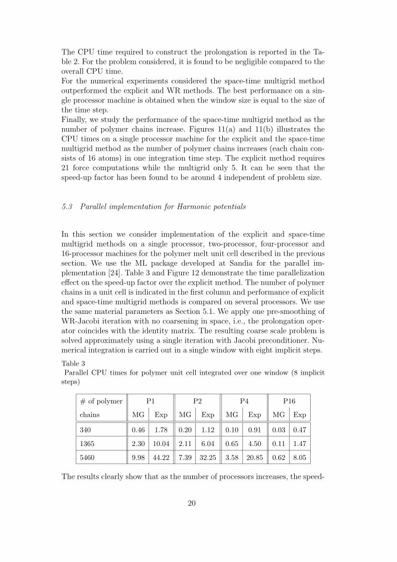
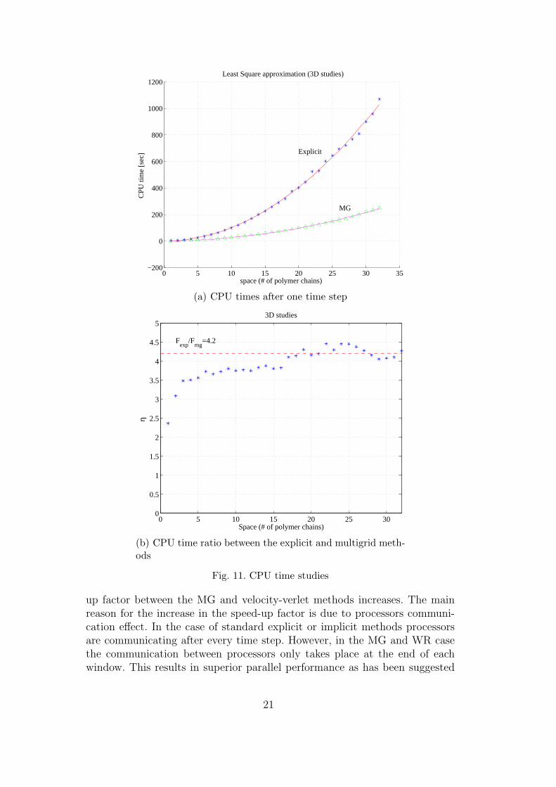
The CPU time required to construct the prolongation is reported in the Ta-ble 2. For the problem considered, it is found to be negligible compared to theoverall CPU time.For the numerical experiments considered the space-time multigrid methodoutperformed the explicit and WR methods. The best performance on a sin-gle processor machine is obtained when the window size is equal to the size ofthe time step.Finally, we study the performance of the space-time multigrid method as thenumber of polymer chains increase. Figures 11(a) and 11(b) illustrates theCPU times on a single processor machine for the explicit and the space-timemultigrid method as the number of polymer chains increases (each chain con-sists of 16 atoms) in one integration time step. The explicit method requires21 force computations while the multigrid only 5. It can be seen that thespeed-up factor has been found to be around 4 independent of problem size.

5.3 Parallel implementation for Harmonic potentials

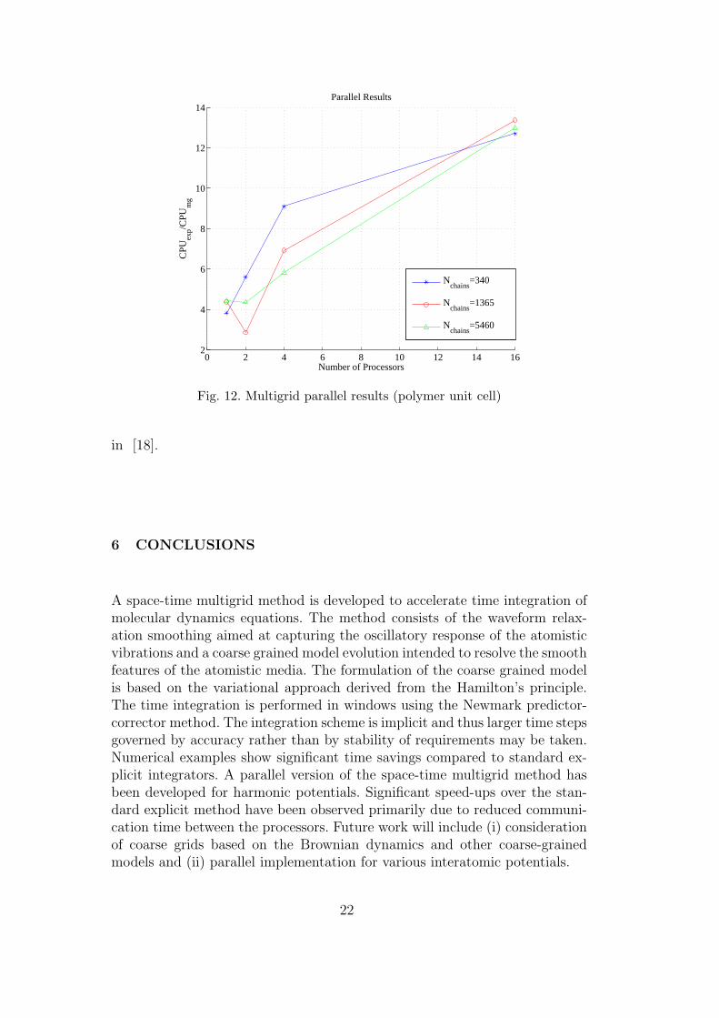
In this section we consider implementation of the explicit and space-timemultigrid methods on a single processor, two-processor, four-processor and16-processor machines for the polymer melt unit cell described in the previoussection. We use the ML package developed at Sandia for the parallel im-plementation [24]. Table 3 and Figure 12 demonstrate the time parallelizationeffect on the speed-up factor over the explicit method. The number of polymerchains in a unit cell is indicated in the first column and performance of explicitand space-time multigrid methods is compared on several processors. We usethe same material parameters as Section 5.1. We apply one pre-smoothing ofWR-Jacobi iteration with no coarsening in space, i.e., the prolongation oper-ator coincides with the identity matrix. The resulting coarse scale problem issolved approximately using a single iteration with Jacobi preconditioner. Nu-merical integration is carried out in a single window with eight implicit steps.

Table 3Parallel CPU times for polymer unit cell integrated over one window (8 implicit

steps)

# of polymer P1 P2 P4 P16

chains MG Exp MG Exp MG Exp MG Exp

340 0.46 1.78 0.20 1.12 0.10 0.91 0.03 0.47

1365 2.30 10.04 2.11 6.04 0.65 4.50 0.11 1.47

5460 9.98 44.22 7.39 32.25 3.58 20.85 0.62 8.05

The results clearly show that as the number of processors increases, the speed-

20

0 5 10 15 20 25 30 35−200

0

200

400

600

800

1000

1200 Least Square approximation (3D studies)

space (# of polymer chains)

CP

U ti

me

[sec

]

MG

Explicit

(a) CPU times after one time step

0 5 10 15 20 25 300

0.5

1

1.5

2

2.5

3

3.5

4

4.5

5

Space (# of polymer chains)

η

Fexp

/Fmg

=4.2

3D studies

(b) CPU time ratio between the explicit and multigrid meth-ods

Fig. 11. CPU time studies

up factor between the MG and velocity-verlet methods increases. The mainreason for the increase in the speed-up factor is due to processors communi-cation effect. In the case of standard explicit or implicit methods processorsare communicating after every time step. However, in the MG and WR casethe communication between processors only takes place at the end of eachwindow. This results in superior parallel performance as has been suggested

21

0 2 4 6 8 10 12 14 162

4

6

8

10

12

14

Number of Processors

CPU

exp/C

PUm

g

Parallel Results

Nchains

=340

Nchains

=1365

Nchains

=5460

Fig. 12. Multigrid parallel results (polymer unit cell)

in [18].

6 CONCLUSIONS

A space-time multigrid method is developed to accelerate time integration ofmolecular dynamics equations. The method consists of the waveform relax-ation smoothing aimed at capturing the oscillatory response of the atomisticvibrations and a coarse grained model evolution intended to resolve the smoothfeatures of the atomistic media. The formulation of the coarse grained modelis based on the variational approach derived from the Hamilton’s principle.The time integration is performed in windows using the Newmark predictor-corrector method. The integration scheme is implicit and thus larger time stepsgoverned by accuracy rather than by stability of requirements may be taken.Numerical examples show significant time savings compared to standard ex-plicit integrators. A parallel version of the space-time multigrid method hasbeen developed for harmonic potentials. Significant speed-ups over the stan-dard explicit method have been observed primarily due to reduced communi-cation time between the processors. Future work will include (i) considerationof coarse grids based on the Brownian dynamics and other coarse-grainedmodels and (ii) parallel implementation for various interatomic potentials.

22

Acknowledgements

The financial supports of National Science Foundation under grants CMS-0310596, 0303902, 0408359 and Sandia National Laboratory under contractDE-ACD4-94AL85000 are gratefully acknowledged. In particular, the authorswish to thank Dr. Ray Tuminaro from Sandia National Laboratory for hisconstructive suggestions

References

[1] D.C. Rapaport. The art of molecular dynamics simulations. Cambridgeuniversity press, 1995.

[2] D. Barash, L. Yang, X. Qian, and T. Schlick. Inherent speedup limita-tions in multiple time step/particle mesh ewald algorithms. Journal ofComputational Chemistry, 24:77–88, 2003.

[3] B. J. Leimkuhler, S. Reich, and R. D. Skeel. Integration methods formolecular dynamics. IMA Volumes in Mathematics and its Applications,82:161–186, 1997.

[4] D. Janezic and B. Orel. Implicit Runge-Kutta method for moleculardynamics integration. Journal of Chemical Information and ComputerSciences, 33:252–257, 1993.

[5] J. Fish and W. Chen. Discrete-to-continuum bridging based on multigridprinciples. Computer Methods in Applied Mechanics and Engineering,193:1693–1711, 2004.

[6] J. Fish and V. Belsky. Multigrid method for periodic heterogeneous mediapart 1: Convergence studies for one-dimensional case. Computer Methodsin Applied Mechanics and Engineering, 126:1–16, 1995.

[7] J. Fish and V. Belsky. Multi-grid method for periodic heterogeneous me-dia part 2: Multiscale modeling and quality control in multidimensionalcase. Computer Methods in Applied Mechanics and Engineering, 126:17–38, 1995.

[8] W. Hackbusch. Multi-grid methods and applications. Springer, 1985.[9] E. Lelarasmee, A. E. Ruehli, and A. L. Sangiovanni-Vincentelli. The

waveform relaxation method for time-domain analysis of large scale inte-grated circuits. IEEE transactions on computer-aided design of integratedcircuits and systems, CAD-1(3):131–145, 1982.

[10] K. Burrage. Parallel and sequential methods for ordinary differential equa-tions. Oxford University Press, 1995.

[11] S. Ta”san and H. Zhang. Fourier-laplace analysis of multigrid waveformrelaxation method for hyperbolic equations. Technical Report ICASE96-53, NASA, 1996.

23

[12] B. Leimkuhler. Timestep acceleration of waveform realxation. SIAMJournal on Numerical Analysis, 35(1):31–50, 1998.

[13] R. Saleh and J. White. Accelerating relaxation algorithms for circuit sim-ulation using waveform-newton and step-size refinement. IEEE Transac-tions on computer-aided design, 9(9):951–958, 1990.

[14] Andrew Lumsdaine and Mark W. Reichelt. Waveform iterative tech-niques for device transient simulation on parallel machines. In Sixth SIAMConference on Parallel Processing for Scientific Computing, Norfolk, VA,1993.

[15] T. J. R. Hughes. The finite element method. Linear static and dynamicfinite element analysis. Prentice-Hall, 1987.

[16] U. Miekkala and O. Nevanlinna. Convergence of dynamic iteration meth-ods for initial value problems. SIAM Journal on Scientific and StatisticalComputing, 8(4):459–482, 1987.

[17] E. Giladi and H. B. Keller. Space time domain decomposition for par-abolic problems. Numerische Mathematik, 93(2):279–313, 2002.

[18] S. Vandewalle. The parallel solution of parabolic partiall differential equa-tions by multigrid waveform relaxation methods. PhD thesis, KatholikeUniversiteit Leuven, 1992.

[19] G. Horton and S. Vandewalle. A space-time multigrid method for par-abolic partial differential equations. SIAM Journal on Scientific and Sta-tistical Computing, 16(4):848–864, 1995.

[20] J. T. Padding and W. J. Briels. Coarse-grained molecular dynamics sim-ulations of polymer melts in transient and steady shear flow. Journal ofChemical Physics, 118(22):10276–10286, 2003.

[21] C. S Peskin and Schlick T. Molecular dynamics by the backward-eulermethod. Communications On Pure and Applied Mathematics, 42:1001–1031, 1989.

[22] J. Fish and W. Chen. Rve-based multilevel method for periodic hetero-geneous media with strong scale mixing. Journal of Engineering Mathe-matics, 46:87–106, 2003.

[23] J. Fish and V. Belsky. Generalized Aggregation Multilevel solver. Interna-tional Journal for Numerical Methods in Engineering, 40(23):4341–4361,1997.

[24] C. Tong and R. S. Tuminaro. ML 2.0 smoothed aggregation user’s guide.Technical Report SAND2001-8028, Sandia National Laboratories, 2000.

24