arX

iv:1

407.

5155

v4 [

cs.L

G]

22 A

ug 2

015

1

Sparse and spurious:dictionary learning with noise and outliers

Remi Gribonval,IEEE Fellow, Rodolphe Jenatton, Francis Bach

Abstract—A popular approach within the signal processingand machine learning communities consists in modelling signalsas sparse linear combinations of atoms selected from alearneddictionary. While this paradigm has led to numerous empir-ical successes in various fields ranging from image to audioprocessing, there have only been a few theoretical argumentssupporting these evidences. In particular, sparse coding,or sparsedictionary learning, relies on a non-convex procedure whose localminima have not been fully analyzed yet. In this paper, weconsider a probabilistic model of sparse signals, and show that,with high probability, sparse coding admits a local minimumaround the reference dictionary generating the signals. Ourstudy takes into account the case of over-complete dictionaries,noisy signals, and possible outliers, thus extending previous worklimited to noiseless settings and/or under-complete dictionaries.The analysis we conduct is non-asymptotic and makes it possibleto understand how the key quantities of the problem, such asthe coherence or the level of noise, can scale with respect tothedimension of the signals, the number of atoms, the sparsity andthe number of observations.

I. I NTRODUCTION

Modelling signals as sparse linear combinations of atomsselected from a dictionary has become a popular paradigm inmany fields, including signal processing, statistics, and ma-chine learning. This line of research has witnessed the devel-opment of several well-founded theoretical frameworks (see,e.g., [44, 45]) and efficient algorithmic tools (see, e.g., [7] andreferences therein).

However, the performance of such approaches hinges onthe representation of the signals, which makes the questionof designing “good” dictionaries prominent. A great deal ofeffort has been dedicated to come up with efficientpredefineddictionaries, e.g., the various types of wavelets [29]. Theserepresentations have notably contributed to many successfulimage processing applications such as compression, denoising

This is a substantially revised version of a first draft that appeared as apreprint titled “Local stability and robustness of sparse dictionary learning inthe presence of noise”, [25].

This work was supported in part by the EU FET- Open programmethrough the SMALL Project under Grant 225913 and in part by the EuropeanResearch Council through the PLEASE Project (ERC-StG-2011-277906) andthe SIERRA project (ERC-StG-2011-239993).

R. Gribonval is with the Institut de Recherche en Systemes Aleatoires (Inria& CNRS UMR 6074), Rennes 35042, France (email: remi.gribonval@inria.fr).

R. Jenatton was with the Laboratoire d’Informatique,Ecole NormaleSuperieure, Paris 75005, France. He is now the Amazon Development CenterGermany, Berlin 10178, Germany (e-mail: jenatton@amazon.com).

F. Bach is with the Laboratoire d’Informatique,Ecole Normale Superieure,Paris 75005, France (e-mail: francis.bach@ens.fr).

Copyright (c) 2015 IEEE. Personal use of this material is permitted.However, permission to use this material for any other purposes must beobtained from the IEEE by sending a request to pubs-permissions@ieee.org.

and deblurring. More recently, the idea of simultaneouslylearning the dictionary and the sparse decompositions of thesignals—also known assparse dictionary learning, or simply,sparse coding—has emerged as a powerful framework, withstate-of-the-art performance in many tasks, including inpaint-ing and image classification (see, e.g., [28] and referencestherein).

Although sparse dictionary learning can sometimes be for-mulated as convex [6, 9], non-parametric Bayesian [47] andsubmodular [27] problems, the most popular and widely useddefinition of sparse coding brings into play a non-convexoptimization problem. Despite its empirical and practicalsuccess, the theoretical analysis of the properties of sparsedictionary learning is still in its infancy. A recent line ofwork[31, 41, 32] establishes generalization bounds which quantifyhow much theexpectedsignal-reconstruction error differs fromthe empirical one, computed from a random and finite-sizesample of signals. In particular, the bounds obtained by Maurerand Pontil [31], Vainsencher et al. [41], Gribonval et al. [21]are non-asymptotic, and uniform with respect to the wholeclass of dictionaries considered (e.g., those with normalizedatoms).

a) Dictionary identifiability.: This paper focuses on acomplementary theoretical aspect of dictionary learning:thecharacterization of local minima of an optimization problemassociated to sparse coding, in spite of the non-convexity ofits formulation. This problem is closely related to the questionof identifiability, that is, whether it is possible torecover areference dictionary that is assumed to generate the observedsignals. Identifying such a dictionary is important when theinterpretation of the learned atoms matters, e.g., in sourcelocalization [12], where the dictionary corresponds to theso-called mixing matrix indicating directions of arrival, in topicmodelling [24], where the atoms of the dictionary are expectedto carry semantic information, or in neurosciences, wherelearned atoms have been related to the properties of the visualcortex in the pioneering work of Field and Olshausen [14].

In fact, characterizing how accurately one can estimatea dictionary through a given learning scheme also mattersbeyond such obvious scenarii where the dictionary intrinsicallycarries information of interest. For example, when learninga dictionary for coding or denoising, two dictionaries areconsidered as perfectly equivalent if they lead to the samedistortion-rate curve, or the same denoising performance.Insuch contexts, learning an ideal dictionary through the directoptimization of the idealized performance measure is likelyto be intractable, and it is routinely replaced by heuristicsinvolving the minimization of proxy, i.e., a better behaved

2

cost function. Characterizing (local) minima of the proxy islikely to help in providing guarantees that such minima existclose to those of the idealized performance measure and, moreimportantly, that they also achieve near-optimal performance.

b) Contributions and related work.:In contrast to earlyidentifiability results in this direction by Georgiev et al.[18], Aharon et al. [4], which focused on deterministic butcombinatorial identifiability conditions with combinatorial al-gorithms, Gribonval and Schnass [19] pioneered the analysisof identifiability using a non-convex objective involving an ℓ1

criterion, in the spirit of the cost function initially proposedby Zibulevsky and Pearlmutter [48] in the context of blindsignal separation. In the case where the reference dictionaryforms a basis, they obtained local identifiability results withnoiseless randomk-sparse signals, possibly corrupted by some“mild” outliers naturally arising with the considered Bernoulli-Gaussian model. Still in a noiseless setting and withoutoutliers, with ak-sparse Gaussian signal model, the analysiswas extended by Geng et al. [17] toover-completedictionaries,i.e., dictionaries composed of more atoms than the dimensionof the signals. Following these pioneering results, a numberof authors have established theoretical guarantees on sparsecoding that we summarize in Table I. Most of the existingresults do not handle noise, and none handles outliers. Inparticular, the structure of the proofs of Gribonval and Schnass[19], Geng et al. [17], hinges on the absence of noise andcannot be straightforwardly transposed to take into accountsome noise.

In this paper, we analyze the local minima of sparse codingin the presence of noise and outliers. For that, we considersparse coding with a regularized least-square cost functioninvolving anℓ1 penalty, under certain incoherence assumptionson the underlying ground truth dictionary and appropriate sta-tistical assumptions on the distribution of the training samples.To the best of our knowledge, this is the first analysis whichrelates to the widely used sparse coding objective functionassociated to the online learning approach of Mairal et al.[28]. In contrast, most of the emerging work on dictionaryidentifiability considers either an objective function based onℓ1 minimization under equality constraints [19, 17], for whichthere is no known efficient heuristic implementation, or on anℓ0 criterion [35] a la K-SVD [4]. More algorithmic approacheshave also recently emerged [37, 5] demonstrating the existenceof provably good (sometimes randomized) algorithms of poly-nomial complexity for dictionary learning. Agarwal et al. [2]combine the best of both worlds by providing a polynomialcomplexity algorithm based on a clever randomized clusteringinitialization [3, 5] followed by alternate optimization based onan ℓ1 minimization principle with equality constraints. Whilethis is a definite theoretical breakthrough, these algorithms areyet to be tested on practical problems, while on open sourceimplementation (SPAMS1) of the online learning approach ofMairal et al. [28] is freely available and has been extensivelyexploited on practical datasets over a range of applications.

c) Main contributions.: Our main contributions can besummarized as follows:

1http://spams-devel.gforge.inria.fr/

1) We consider the recovery of a dictionary withp atomsD

o ∈ Rm×p using ℓ1-penalized formulations with

penalty factorλ > 0, given a training set ofn signalsgathered in a data matrixX ∈ R

m×n. This is detailed inSection II-A.

2) We assume a general probabilistic model of sparse sig-nals, where the data matrixX ∈ R

m×n is generated asD

oA

o plus additive noiseε. Our model, described inSection II-C, corresponds to ak-sparse support with loosedecorrelation assumptions on the nonzero coefficients. Itis closely connected to theΓk,C model of Arora et al.[5, Definition 1.2]. In particular, unlike in independentcomponent analysis (ICA) and in most related work,noindependence is assumed between nonzero coefficients.

3) We show that under deterministic (cumulative)coherence-based sparsity assumptions (see Section II-D)the minimized cost function has a guaranteed localminimum around the generating dictionaryDo with highprobability.

4) We also prove support and coefficient recovery, which isimportant for blind source separation.

5) Our work makes it possible to better understand:

a) how small the neighborhood around the referencedictionary can be, i.e., tending to zero as the noisevariance goes to zero.

b) how many signalsn are sufficient to hope for theexistence of such a controlled local minimum, i.e.,n =Ω(mp3). In contrast to several recent results [35, 5, 36]where the sample complexity depends on the targetedresolutionr such that‖D−D

o‖ 6 r, our main samplecomplexity estimates areresolution-independentin thenoiseless case. This is similar in nature to the bettersample complexity resultsn = Ω(p2 log p) obtainedby Agarwal et al. [2] for a polynomial algorithm ina noiseless context, orn = Ω(p logmp) obtained byAgarwal et al. [3] for Rademacher coefficients. This isachieved through a precise sample complexity analysisusing Rademacher averages and Slepian’s lemma. Inthe presence of noise, a factor1/r2 seems unavoidable[35, 5, 36].

c) what sparsity levels are admissible. Our main result isbased on the cumulative coherence (see Section II-D)µk(D

o) 6 1/4. It also involves a condition that re-stricts our analysis to overcomplete dictionaries wherep . m2, where previous works seemingly apply tovery overcomplete settings. Intermediate results onlyinvolve restricted isometry properties. This may allowfor much larger values of the sparsity levelk, and moreovercompleteness, but this is left to future work.

d) what level of noise and outliers appear as manageable,with a precise control of the admissible “energy”of these outliers. While a first naive analysis wouldsuggest a tradeoff between the presence of outliersand the targeted resolutionr, we conduct a tailoredanalysis that demonstrates the existence of aresolution-independentthreshold on the relative amount of out-liers to which the approach is robust.

3

Reference Ove

rcom

plet

e

Noi

se

Out

liers

Glo

bal

min

/al

gori

thm

Pol

ynom

ial

algo

rith

m

Exa

ct(n

ono

ise,

noou

tlier

,nfin

ite)

Sam

ple

com

plex

ity(n

ono

ise)

Adm

issi

ble

spar

sity

for

exact

reco

very

Coe

ffici

ent

mod

el(m

ain

char

acte

rist

ics)

Georgiev et al. [18] k = m− 1,Combinatorial approach X X X m

(

pm−1

)

δm(Do) < 1 CombinatorialAharon et al. [4]Combinatorial approach X X X (k + 1)

(

pk

)

δ2k(Do) < 1 Combinatorial

Gribonval and Schnass [19] km

< Bernoulli(k/p)

ℓ1 criterion X m2 logmk

1− ‖D⊤D− I‖2,∞ -Gaussian

Geng et al. [17] k-sparseℓ1 criterion X X kp3 O(1/µ1(D

o)) -GaussianSpielman et al. [37] Bernoulli(k/p)ℓ0 criterion X X m logm O(m) -Gaussian orER-SpUD (randomized) P (X) X X m2 log2 m O(

√m) -Rademacher

Schnass [35] ‖D−Do‖2,∞ “Symmetric

K-SVD criterion(unit norm tight frames only)

X X 6 r =O(pn−1/4)

mp3 O(1/µ1(Do)) decaying”:

αj = ǫjaσ(j)

Arora et al. [5] ‖D−Do‖2,∞ p2 log p

k2 O(

min( 1µ1(Do) logm

, k-sparse

Clustering (randomized) X X P (X) X 6 r +p log p ·(

k2+log 1r

)

p2/5)

1 6 |αj | 6 C

Agarwal et al. [3] O(

min(1/√

µ1(Do), k-sparseClustering (randomized) &ℓ1

X P (X) X X p logmp m1/5, p1/6))

(+ dynamic range)-Rademacher

Agarwal et al. [2] O(

min(1/√

µ1(Do), k-sparseℓ1 optim with AltMinDict &randomized clustering init.

X P (X) X X p2 log p m1/9, p1/8))

- i.i.d.α 6 |αj | 6 M

Schnass [36] ‖D−Do‖2,∞ “Symmetric

Response maxim. criterion X X 6 r mp3kr2

O(1/µ1(Do)) decaying”

This contribution ‖D−Do‖F k-sparse,

Regularizedℓ1 criterion withpenalty factorλ

X X X 6 r = O(λ)Xfor λ → 0

mp3 µk(Do) 6 1/4 α 6 |αj |,

‖α‖2 6 Mα

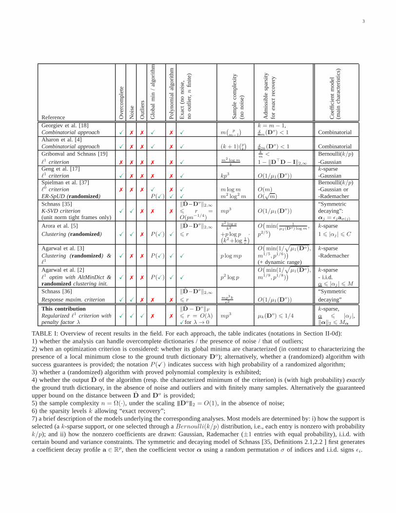
TABLE I: Overview of recent results in the field. For each approach, the table indicates (notations in Section II-0d):1) whether the analysis can handle overcomplete dictionaries / the presence of noise / that of outliers;2) when an optimization criterion is considered: whether its global minima are characterized (in contrast to characterizing thepresence of a local minimum close to the ground truth dictionary D

o); alternatively, whether a (randomized) algorithm withsuccess guarantees is provided; the notationP (X) indicates success with high probability of a randomized algorithm;3) whether a (randomized) algorithm with proved polynomialcomplexity is exhibited;4) whether the outputD of the algorithm (resp. the characterized minimum of the criterion) is (with high probability)exactlythe ground truth dictionary, in the absence of noise and outliers and with finitely many samples. Alternatively the guaranteedupper bound on the distance betweenD andDo is provided;5) the sample complexityn = Ω(·), under the scalingDo2 = O(1), in the absence of noise;6) the sparsity levelsk allowing “exact recovery”;7) a brief description of the models underlying the corresponding analyses. Most models are determined by: i) how the support isselected (ak-sparse support, or one selected through aBernoulli(k/p) distribution, i.e., each entry is nonzero with probabilityk/p); and ii) how the nonzero coefficients are drawn: Gaussian, Rademacher (±1 entries with equal probability), i.i.d. withcertain bound and variance constraints. The symmetric and decaying model of Schnass [35, Definitions 2.1,2.2 ] first generatesa coefficient decay profilea ∈ R

p, then the coefficient vectorα using a random permutationσ of indices and i.i.d. signsǫi.

4

II. PROBLEM STATEMENT

We introduce in this section the material required to defineour problem and state our results.

d) Notations.: For any integerp, we define the setJ1; pK , 1, . . . , p. For all vectorsv ∈ R

p, we denoteby sign(v) ∈ −1, 0, 1p the vector such that itsj-th entry[sign(v)]j is equal to zero ifvj = 0, and to one (respectively,minus one) ifvj > 0 (respectively,vj < 0). The notationsA

⊤ and A+ denote the transpose and the Moore-Penrose

pseudo-inverse of a matrixA. We extensively manipulatematrix norms in the sequel. For any matrixA ∈ R

m×p, wedefine its Frobenius norm by‖A‖F , [

∑mi=1

∑pj=1 A

2ij ]

1/2;similarly, we denote the spectral norm ofA by A2 ,max‖x‖261 ‖Ax‖2, we refer to the operatorℓ∞-norm asA∞ , max‖x‖∞61 ‖Ax‖∞ = maxi∈J1;mK

∑pj=1 |Aij |,

and we denote‖A‖1,2 ,∑

j∈J1;pK ‖aj‖2 with aj the j-th

column ofA. In several places we will exploit the fact thatfor any matrixA we have

A2 6 ‖A‖F .

For any square matrixB ∈ Rn×n, we denote bydiag(B) ∈

Rn the vector formed by extracting the diagonal terms ofB,

and conversely, for anyb ∈ Rn, we useDiag(b) ∈ R

n×n

to represent the (square) diagonal matrix whose diagonalelements are built from the vectorb. Denote off(A) ,A−Diag(diag(A)) the off-diagonal part ofA, which matchesA except on the diagonal where it is zero. The identity matrixis denotedI.

For anym×p matrixA and index setJ ⊂ J1; pK we denoteby AJ the matrix obtained by concatenating the columns ofA

indexed byJ. The number of elements or size ofJ is denoted|J|, and its complement inJ1; pK is denotedJc. Given a matrixD ∈ R

m×p and a support setJ such thatDJ has linearlyindependent columns, we define the shorthands

GJ , GJ(D) , D⊤J DJ

HJ , HJ(D) , G−1J

PJ , PJ(D) , DJD+J = DJHJD

⊤J ,

respectively the Gram matrix ofDJ and its inverse, andthe orthogonal projector onto the span of the columns ofD

indexed byJ.For any functionh(D) we define∆h(D′;D) , h(D′) −

h(D). Finally, the ball (resp. the sphere) of radiusr > 0centered onD in R

m×p with respect to the Frobenius normis denotedB(D; r) (resp.S(D; r)).

The notationa = O(b), or a . b, indicates the existence ofa finite constantC such thata 6 Cb. Vice-versa,a = Ω(b),or a & b, meansb = O(a), anda ≍ b means thata = O(b)andb = O(a) hold simultaneously.

A. Background material on sparse coding

Let us consider a set ofn signalsX , [x1, . . . ,xn] ∈R

m×n each of dimensionm, along with a dictionaryD ,[d1, . . . ,dp] ∈ R

m×p formed of p columns called atoms—also known as dictionary elements. Sparse coding simultane-ously learnsD and a set ofn sparsep-dimensional vectors

A , [α1, . . . ,αn] ∈ Rp×n, such that each signalxi can be

well approximated byxi ≈ Dαi for i in J1;nK. By sparse, wemean that the vectorαi hask ≪ p non-zero coefficients, sothat we aim at reconstructingxi from only a few atoms. Beforeintroducing the sparse coding formulation [33, 48, 28], weneed some definitions. We denote byg : Rp → R

+ a penaltyfunction that will typically promote sparsity.

Definition 1. For any dictionaryD ∈ Rm×p and signalx ∈

Rm, we define

Lx(D,α) , 12‖x−Dα‖22 + g(α) (1)

fx(D) , infα∈Rp

Lx(D,α). (2)

Similarly for any set ofn signalsX , [x1, . . . ,xn] ∈ Rm×n,

we introduce

FX(D) , 1n

n∑

i=1

fxi(D). (3)

Based on problem (2) with theℓ1 penalty,

g(α) , λ‖α‖1, (4)

refered to as Lasso in statistics [38], and basis pursuit insignal processing [11], the standard approach to perform sparsecoding [33, 48, 28] solves the minimization problem

minD∈D

FX(D), (5)

where the regularization parameterλ in (4) controls thetradeoff between sparsity and approximation quality, whileD ⊆ R

m×p is a compact constraint set; in this paper,Ddenotes the set of dictionaries with unitℓ2-norm atoms, alsocalled theoblique manifold[1], which is a natural choice insignal and image processing [28, 19, 34, 39]. Note howeverthat other choices for the setD may also be relevant dependingon the application at hand (see, e.g., Jenatton et al. [24] wherein the context of topic models, the atoms inD belong to theunit simplex). The sample complexity of dictionary learningwith general constraint sets is studied by Maurer and Pontil[31], Gribonval et al. [21] for various families of penaltiesg(α).

B. Main objectives

The goal of the paper is to characterize some local minimaof the functionFX with the ℓ1 penalty, under a generativemodel for the signalsxi. Throughout the paper, the mainmodel we consider is that of observed signals generatedindependentlyaccording to a specified probabilistic model.The signals are typically drawn asxi , D

oαi + εi whereD

o is a fixed reference dictionary,αi is a sparse coefficientvector, andεi is a noise term. The specifics of the underlyingprobabilistic model, and its possible contamination without-liers are considered in Section II-C. Under this model, we canstate more precisely our objective: we want to show that, forlarge enoughn,

P(

FX has a local minimum in a “neighborhood” ofDo)

≈ 1.

We loosely refer to a “neighborhood” since in our regularizedformulation, a local minimum is not necessarily expected to

5

appear exactly atDo. The proper meaning of this neighbor-hood is in the sense of the Frobenius distance‖D − D

o‖F .Other metrics can be envisioned and are left as future work.How largen should be for the results to hold is related to thenotion of sample complexity.

e) Intrinsic ambiguities of sparse coding.:Importantly,we so far referred toDo asthereference dictionary generatingthe signals. However, and as already discussed by Gribonvaland Schnass [19], Geng et al. [17] and more generally in therelated literature on blind source separation and independentcomponent analysis [see, e.g., 12], it is known that theobjective of (5) is invariant by sign flips and permutationsof the atoms. As a result, while solving (5), we cannothope to identify the specificDo. We focus instead on thelocal identifiability of the wholeequivalence classdefinedby the transformations described above. From now on, wesimply refer toDo to denote one element of this equivalenceclass. Also, since these transformations arediscrete, our localanalysis is not affected by invariance issues, as soon as we aresufficiently close to some representant ofD

o.

C. The sparse and the spurious

The considered training set is composed of two types ofvectors:the sparse, drawn i.i.d. from a distribution generating(noisy) signals that are sparse in the dictionaryD

o; and thespurious, corresponding tooutliers.

1) The sparse: probabilistic model of sparse signals (in-liers): Given a reference dictionaryDo ∈ D, each (inlier)signalx ∈ R

m is built independentlyin three steps:• Support generation: Draw uniformly without replace-

mentk atoms out of thep available inDo. This procedurethus defines a supportJ ⊂ J1; pK whose size is|J| = k.

• Coefficient vector: Draw a sparse vectorαo ∈ Rp

supported onJ (i.e., with αoJc = 0).

• Noise: Eventually generate the signalx = Doαo + ε.

The random vectorsαoJ and ε satisfy the following assump-

tions, where we denoteso = sign(αo).

Assumption A (Basic signal model).

E

αoJ[α

oJ]

⊤ | J

= Eα2 · I (6)

coefficient whiteness

E

soJ [s

oJ ]

⊤ | J

= I (7)

sign whiteness

E

αoJ[s

oJ ]

⊤ | J

= E|α| · I (8)

sign/coefficient decorrelation

E

ε[αoJ]

⊤ | J

= E

ε[soJ ]⊤ | J

= 0 (9)

noise/coefficient decorrelation

E

εε⊤|J

= Eǫ2 · I (10)

noise whiteness

In light of these assumptions we define the shorthand

κα ,E|α|√Eα2

. (11)

By Jensen’s inequality, we haveκα 6 1, with κα = 1corresponding to the degenerate situation whereαJ almost

surely has all its entries of the same magnitude, i.e., withthe smallest possible dynamic range. Conversely,κα ≪ 1corresponds to marginal distributions of the coefficients witha wide dynamic range. In a way,κα measures the typical“flatness” ofα (the largerκα, the flatter the typicalα)

A boundednessassumption will complete Assumption A tohandle sparse recovery in our proofs.

Assumption B (Bounded signal model).

P(minj∈J

|αoj | < α | J) = 0, for someα > 0 (12)

coefficient threshold

P(‖αo‖2 > Mα) = 0, for someMα (13)

coefficient boundedness

P(‖ε‖2 > Mε) = 0, for someMε. (14)

noise boundedness

Remark 1. Note that neither Assumption A nor Assumption Brequires that the entries ofαo indexed byJ be i.i.d. Infact, the stable and robust identifiability ofDo from thetraining set X rather stems from geometric properties ofthe training set (its concentration close to a union of low-dimensional subspaces spanned by few columns ofD

o) thanfrom traditional independent component analysis (ICA). Thiswill be illustrated by a specific coefficient model (inspiredbythe symmetric decaying coefficient model of Schnass [35]) inExample 1.

To summarize, the signal model is parameterized by thesparsityk, the expected coefficient energyE α2, the minimumcoefficient magnitudeα, maximum normMα, and the flatnessκα. These parameters are interrelated, e.g.,α

√k 6 Mα.

a) Related models:The Bounded model above is relatedto theΓk,C model of Arora et al. [5] (which also covers [3, 2]):in the latter, our assumptions (12)-(13) are replaced by1 6|αj | 6 C. Note that theΓk,C model of Arora et al. [5] doesnot assume that the support is chosen uniformly at random(among all k-sparse sets) and some mild dependencies areallowed. Alternatives to (13) with a control on‖α‖q for some0 < q 6 ∞ can easily be dealt with through appropriatechanges in the proofs, but we chose to focus onq = 2 forthe sake of simplicity. Compared to early work in the fieldconsidering a Bernoulli-Gaussian model [19] or ak-sparseGaussian model [17], Assumptions A & B are rather genericand do not assume a specific shape of the distributionP(α).In particular, the conditional distribution ofαJ given J maydepend onJ, provided its “marginal moments”E α2 andE |α|satisfy the expressed assumptions.

2) The spurious:outliers: In addition to a set ofnin

inliers drawn i.i.d. as above, the training set may containnout

outliers, i.e., training vectors that may have completely distinctproperties and may not relate in any manner to the referencedictionaryDo. Since the considered cost functionFX(D) isnot altered when we permute the columns of the matrixX

representing the training set, without loss of generality we willconsider thatX = [Xin,Xout]. As we will see, controllingthe ratio ‖Xout‖2F /nin of the total energy of outliers to thenumber of inliers will be enough to ensure that the local

6

minimum of the sparse coding objective function is robustto outliers. While this control does not require any additionalassumptions, the ratio‖Xout‖2F /nin directly impacts the errorin estimating the dictionary (i.e., the local minimum inD isfurther away fromD

o). With additional assumptions (namelythat the reference dictionary is complete), we show that if‖Xout‖1,2/nin is sufficiently small, then our upper bound onthe distance from the local minimum toDo remains valid.

D. The dictionary: cumulative coherence and restricted isom-etry properties

Part of the technical analysis relies on the notion ofsparserecovery. A standard sufficient support recovery condition isreferred to as theexact recovery conditionin signal pro-cessing [16, 40] or theirrepresentability condition(IC) inthe machine learning and statistics communities [44, 46].It is a key element to almost surely control the supportsof the solutions ofℓ1-regularized least-squares problems. Tokeep our analysis reasonably simple, we will impose theirrepresentability conditionvia a condition on thecumulativecoherenceof the reference dictionaryDo ∈ D, which is astronger requirement [43, 15]. This quantity is defined (see,e.g., [16, 13]) for unit-norm columns (i.e., on the obliquemanifoldD) as

µk(D) , sup|J|6k

supj /∈J

‖D⊤J d

j‖1. (15)

The termµk(D) gives a measure of the level of correlationbetween columns ofD. It is for instance equal to zero inthe case of an orthogonal dictionary, and exceeds one ifD

contains two colinear columns. For a given dictionaryD,the cumulative coherence ofµk(D) increases withk, andµk(D) 6 kµ1(D) whereµ1(D) = maxi6=j |〈di,dj〉| is theplain coherence ofD.

For the theoretical analysis we conduct, we consider adeterministic assumption based on the cumulative coherence,slightly weakening the coherence-based assumption consid-ered for instance in previous work on dictionary learning [19,17]. Assuming thatµk(D

o) < 1/2 wherek is the level ofsparsity of the coefficient vectorsαi, an important step will beto show that such an upper bound onµk(D

o) loosely transfersto µk(D) provided thatD is close enough toDo, leading tolocally stable exact recovery results in the presence of boundednoise(Proposition 3).

Many elements of our proofs rely on a restricted isometryproperty (RIP), which is known to be weaker than the co-herence assumption [43]. By definition therestricted isometryconstantof orderk of a dictionaryD, δk(D) is the smallestnumberδk such that for any support setJ of size |J| = k andz ∈ R

k,

(1− δk) ‖z‖22 6 ‖DJz‖22 6 (1 + δk) ‖z‖22. (16)

In our context,the best lower bound and best upper bound willplay significantly different roles, so we define them separatelyas δk(D) and δk(D), so thatδk(D) = max(δk(D), δk(D)).Both can be estimated by the cumulative coherence asδk(D) 6 µk−1(D) by Gersgorin’s disc theorem [40]. Possible

extensions of this work that would fully relax the incoherenceassumption and only rely on the RIP are discussed in Sec-tion V.

III. M AIN RESULTS

Our main results, described below, show that under appro-priate scalings of the dictionary dimensionsm, p, number oftraining samplesn, and model parameters, the sparse codingproblem (5) admits a local minimum in a neighborhood ofD

o of controlled size, for appropriate choices of the regular-ization parameterλ. The main building blocks of the results(Propositions 1-2-3) and the high-level structure of theirproofsare given in Section IV. The most technical lemmata arepostponed to the Appendix.

A. Stable local identifiability

We begin with asymptotic results (n being infinite), in theabsence of outliers.

Theorem 1 (Asymptotic results, bounded model, no outlier).Consider the following assumptions:

• Coherence and sparsity level:considerDo ∈ D and ksuch that

µk(Do) 6 1/4 (17)

k 6p

16(Do2 + 1)2. (18)

• Coefficient distribution: assume the Basic & Boundedsignal model (Assumptions A & B) and

E α2

MαE |α| > 84 · (Do2 + 1) ·

kp · ‖[Do]⊤Do − I‖F

1− 2µk(Do).

(19)

This impliesCmin < Cmax where we define

Cmin , 24κ2α · (Do

2 + 1) · kp· ‖[Do]⊤Do − I‖F ,

(20)

Cmax ,2

7· E |α|Mα

· (1− 2µk(Do)). (21)

• Regularization parameter: consider a small enoughregularization parameter,

λ 6α

4. (22)

Denotingλ , λE |α| , this impliesCmax · λ 6 0.15.

• Noise level:assume a small enough relative noise level,

Mε

Mα

<7

2· (Cmax − Cmin) · λ. (23)

Then, for any resolutionr > 0 such that

Cmin · λ < r < Cmax · λ, (24)

andMε

Mα

<7

2

(

Cmax · λ− r)

, (25)

the functionD ∈ D 7→ E FX(D) admits a local minimumDsuch that‖D−D

o‖F < r.

7

no noise / no outliers no outliers many small outliers few large outliers

Fig. 1: Noise and outliers: illustration with three atoms intwo dimensions (blue crosses: inliers, red circles:outliers).

Remark 2 (Limited over-completeness ofDo). It is perhapsnot obvious how strong a requirement is assumption(19). Onthe one hand, its left hand side is easily seen to be less thanone (and as seen above can be made arbitarily close to onewith appropriate coefficient distribution). On the other handby the Welsh bound‖[Do]⊤Do−Id‖F ≥

√

p(p−m)/m, theboundDo2 ≥ ‖Do‖F /

√m =

√

p/m, and the assumptionµk(D

o) 6 1/4, its right hand side is bounded from belowby Ω(k

√

(p−m)/m2). Hence, a consequence of assump-tion (19) is that Theorem 1 only applies to dictionaries withlimited over-completeness, withp . m2. This is likely to be anartifact from the use of coherence in our proof, and a degreeof overcompletenessp = O(m2) covers already interestingpractical settings: for example [28] considerm = (8 × 8)patches withp = 256 atoms< m2 = 642 = 4096)

Since kp · ‖[Do]⊤Do − I‖F 6 kµ1(D

o) and µk(Do) 6

kµ1(Do), a crude upper bound on the rightmost factor

in (19) is kµ1(Do)/(1− 2kµ1(D

o)), which appears in manycoherence-based sparse-recovery results.

1) Examples:Instantiating Theorem 1 on a few exampleshighlights the strength of its main assumptions.

Example 1 (Incoherent pair of orthonormal bases). WhenDo

is an incoherent dictionary inRm×p, i.e., a dictionary with(plain) coherenceµ = µ1(D

o) ≪ 1, we have the estimates[40] µk(D

o) 6 kµ and

‖[Do]⊤Do − I‖F 6√

p(p− 1)µ2 6 pµ.

Assumption(17) therefore holds as soon ask 6 1/(4µ). In thecase wherep = 2m andD

o is not only incoherent but also aunion of two orthonormal bases, we further haveDo2 =

√2

hence assumption(18) is fulfilled as soon ask 6 p/100 =m/50. Moreover, the right hand side in(19) reads

84 · (Do+1) ·

kp · ‖[Do]⊤Do − I‖F

1− 2µk(Do)6

203kµ

1− 2kµ6 406kµ,

and assumption(19) holds provided thatEα2/(MαE|α|) ex-ceeds this threshold. We discuss below concrete signal settingswhere this condition can be satisfied:

• i.i.d. bounded coefficient model: on the one hand,consider nonzero coefficients drawn i.i.d. withP(|αj | <α|j ∈ J) = 0. The almost-sure upper-boundMα on‖α‖2 implies the existence ofα ≥ α such thatP(|αj | >α|j ∈ J) = 0. As an example, consider coefficientsdrawn i.i.d. with P(αj = ±α|j ∈ J) = π ∈ (0, 1)and P(αj = ±α|j ∈ J) = 1 − π. For large α we

haveEα2 = πα2 + (1 − π)α2 ≍ πα2, E|α| ≍ πα, andMα =

√kα. This yields

limα→∞

Eα2/(MαE|α|) = 1/√k,

This shows the existence of a coefficient distributionsatisfying (19) as soon as406kµ < 1/

√k, that is

to say k < 1/(406µ)2/3. In the maximally incoherentcase, for largep, we haveµ = 1/

√m ≍ p−1/2, and

conditions(17)-(18)-(19) read k = O(p1/3).• fixed amplitude profile coefficient model:on the other

hand, completely relax the independence assumptionand consider essentially the coefficient model introducedby Schnass [35] whereαj = ǫjaσ(j) with i.i.d. signsǫj such thatP(ǫj = ±1) = 1/2, a random permutationσ of the index setJ, and a a given vector with entriesaj ≥ α, j ∈ J. This yields

Eα2/(MαE|α|) = 1k‖a‖

22/(‖a‖2 · 1k‖a‖1) = ‖a‖2/‖a‖1,

which can be made arbitrarily close to one even withthe constraintaj ≥ α, j ∈ J. This shows the existenceof a coefficient distribution satisfying(19) as soon as406kµ < 1, a much less restrictive condition leadingto k = O(p1/2). The reader may notice that suchdistributions concentrate most of the energy ofα on justa few coordinates, so in a sense such vectors are muchsparser thank-sparse.

Example 2 (Spherical ensemble). ConsiderDo ∈ Rm×p a

typical draw from the spherical ensemble, that is a dictionaryobtained by normalizing a matrix with standard independentGaussian entries. As discussed above, condition(19) imposesoverall dimensionality constraintsp . m2. Moreover, usingusual results for such dictionaries [see, e.g., 10], the conditionin (17) is satisfied as soon asµk 6 kµ1 ≈ k

√log p/

√m =

O(1), i.e., k = O(√

m/ log p), while the condition in(18) issatisfied as long ask = O(m) (which is weaker).

2) Noiseless case: exact recovery:In the noiseless case(Mε = 0), (23) imposes no lower bound on admissibleregularization parameter. Hence, we deduce from Theorem 1that a local minimum ofE FX(·) can be found arbitrarily closeto D

o, provided that the regularization parameterλ is smallenough. This shows that the reference dictionaryD

o itself is infact a local minimum of the problem considered by Gribonvaland Schnass [19], Geng et al. [17],

minD∈D

F 0X(D) whereF 0

X(D) , minA:DA=X

‖A‖1. (26)

8

Note that here we consider a different random sparse signalmodel, and yet recover the same results together with a newextension to the noisy case.

3) Stability to noise: In the presence of noise, condi-tions (22) and (23) respectively impose an upper and a lowerlimit on admissible regularization parameters, which are onlycompatible for small enough levels of noise

Mε . α(1− 2µk(Do)).

In scenarios whereCmin ≪ Cmax (i.e., when the left handside in (19) is large enough compared to its right hand side),admissible regularization parameters are bounded from belowgiven (23) asλ & Mε

MαCmax

, therefore limiting the achievable“resolution” r to

r > Cminλ &Mε

Mα

· Cmin

Cmax

≍ Mε√E α2

· κα · Do2 ·

kp · ‖[Do]⊤Do − I‖F

1− 2µk(Do).

(27)

Hence, with enough training signals and in the absence ofoutliers, the main resolution-limiting factors are

• the relative noise levelMε/√E α2: the smaller the better;

• the level of typical “flatness” ofα as measured byκα:the peakier (the smallerκα) the better;

• the coherence of the dictionary as measured jointly byµk(D

o) and kp · ‖[Do]⊤Do − I‖F : the least coherent the

better.

Two other resolution-limiting factors are the finite numberof training samplesn and the presence of outliers, which wenow discuss.

B. Robust finite sample results

We now trade off precision for concision and express finitesample results with two non-explicit constantsC0 and C1.Their explicit expression in terms of the dictionary and signalmodel parameters can be tracked back by the interested readerin the proof of Theorem 2 (Section IV-G), but they are leftaside for the sake of concision.

Theorem 2 (Robust finite sample results, bounded model).Consider a dictionaryDo ∈ D and a sparsity levelk satisfyingthe assumptions(17)-(18) of Theorem 1, and the Basic &Bounded signal model (Assumptions A & B) with parame-ters satisfying the assumption(19). There are two constantsC0, C1 > 0 independent of all considered parameters with thefollowing property.

Given a reduced regularization parameterλ and a noiselevel satisfying assumptions(22) and (23), a radius r satis-fying (24) and (25), and a confidence levelx > 0, whennin

training samples are drawn according to the Basic & Boundedsignal model with

nin > C0 · (mp+ x) · p2 ·(

M2

α

E‖α‖2

2

)2

·

r+

(

Mε

Mα

+λ

)

+

(

Mε

Mα

+λ

)

2

r−Cmin·λ

2

,

(28)

we have: with probability at least1− 2e−x, the functionD ∈D 7→ FX(D) admits a local minimumD such that‖D −D

o‖F < r. Moreover, this is robust to the addition of outliersXout provided that

‖Xout‖2

F

nin6 E‖α‖22 ·

[

14p ·

(

1− Cmin·λr

)

− C1

√

(mp+x)nin

]

· r2.(29)

As soon as the dictionary is coherent, we haveCmin 6= 0,hence the constraint(24) implies that the right hand sideof (29) scales asO(r2) = O(λ2). In the noiseless case,this imposes a tradeoff between the seeked resolutionr, thetolerable total energy of outliers, and the number of inliers.With a more refined argument, we obtain the alternativecondition

‖Xout‖1,2

nin6 3

√kE ‖α‖2

2

E|α| ·[

1p ·(

1− Cmin·λr

)

− C1

√

(mp+x)nin

]

· rλ· (Ao)3/2

18p3/2 ,

(30)

where Ao is the lower frame bound ofDo, i.e., such thatAo‖x‖22 6 ‖(Do)⊤x‖22 for any signalx.

The factorM2α/E ‖α‖22 = “ sup ‖α‖22′′/E ‖α‖22 in the

right hand side of (28) is always greater than 1, but typicallyremains bounded (note that if the distribution ofα allowsoutliers, they could be treated within the outlier model). Inthe symmetric decaying model of Schnass [35] whereα isa randomly permuted and signed flipped version of a givenvector, this factor is equal to one.

Even though the robustness to outliers is expressed in (29)as a control of‖Xout‖2F /nin, it should really be consid-ered as a control of anoutlier to inlier energy ratio:‖Xout‖2F /[ninE ‖α‖22], and similarly with a proper adaptationin (30). One may notice that the robustness to outliers ex-pressed in Theorem 2 is somehow a “free” side-effect of theconditions that hold on inliers with high probability, rather thanthe result of a specific design of the cost functionFX(D).

1) Example: orthonormal dictionary:Considerp = m andD

o an orthonormal dictionary inRm×p. Sinceµk(Do) = 0,

Do2 = 1 and‖[Do]⊤Do−I‖F = 0, assumption (18) reads2

k 6 p/64, assumptions (17) and (19) impose no constraint,andCmin = 0. Moreover, the reader can check that ifMε <λ 6 α/4, then (22)-(25) hold for0 < r < 2(λ−Mε)

7Mα

.• Low-noise regime: if Mε < α/4 and k 6 p/64, then

choosingMε < λ 6 α/4 yields:– by Theorem 1 (the limit of largen), EFX(D) admits

a local minimumexactly atDo;– by Theorem 2,even though the regularization pa-

rameter cannot be made arbitrarily small, we obtainthat for any confidence levelx > 0 and arbitrarysmall precision r > 0, FX(D) admits a localminimum within radiusr aroundDo with probabilityat least1− 2e−x provided that

n = Ω(

(mp3 + xp2)(

Mε/Mα

r

)2 )

.

2Improved constants in Theorem 1 are achievable when specializing toorthonormal dictionaries, they are left to the reader.

9

While the orthogonality of the dictionary remarkablyallows to achieve an arbitrary precision despite thepresence of noise, we still have to pay a price forthe presence of noise through a resolution-dependentsample complexity.

• Noiseless regime (Mε = 0): with λ ≍ r, an arbitraryresolution r is reached with aresolution independentnumber of training samples

n = Ω(mp3 + xp2).

This is robust to outliers provided‖Xout‖1,2/nin does notexceed aresolution independentthreshold.

The case of orthonormal dictionaries is somewhat special inthe sense that orthonormality yieldsCmin = 0 and breaksthe forced scalingr ≍ λ otherwise imposed by (24). Belowwe discuss in more details the more generic case of non-orthonormal dictionaries in the noiseless case.

2) Noiseless case: exact recovery and resolution indepen-dent sample complexity:Consider now the noiseless case(Mε = 0) without outlier (Xout = 0). In general we haveCmin > 0 hence the best resolutionr > 0 guaranteed by The-orem 1 in the asymptotic regime isr = rmin , Cmin · λ > 0.When Cmax > 2Cmin, Theorem 2 establishes that the onlyslightly worse resolutionr = 2rmin can be achieved withhigh probability with a number of training samplesn whichis resolution independent. More precisely (28) indicates thatwhenM2

α/E ‖α‖22 ≈ 1, it is sufficient to have a number oftraining samples

n = Ω(mp3)

to ensure the existence of a local minimum within a radiusraround the ground truth dictionaryDo, wherethe resolutionr can be made arbitrarily fine by choosingλ small enough.This recovers the known fact that, with high probability, thefunctionF 0

X(D) defined in (26) has a local minimumexactly

at Do, as soon asn = Ω(mp3). Given our boundedness

assumption, the probabilistic decay ase−x is expected andshow that as soon asn ≥ Ω(mp3), the infinite sample resultis reached quickly.

In terms of outliers, both (29) and (30) provide a controlof the admissible “energy” of outliers. Without additionalassumption onDo, the allowed energy of outliers in (29)has a leading term inr2, i.e., to guarantee a high precision,we can only tolerate a small amount of outliers as measuredby the ratio‖Xout‖2F/nin. However, when the dictionaryDo

is complete –a rather mild assumption– the alternate ratio‖Xout‖1,2/nin does not need to scale with the targeted res-olution r for r = 2Cminλ. In the proof, this corresponds toreplacing the control of the minimized objective function bythat of its variations.

The above described resolution-independent results are ofcourse specific to the noiseless setting. In fact, as describedin Section III-A3, the presence of noise when the dictionaryis not orthonormal imposes an absolute limit to the resolutionr > rmin we can guarantee with the techniques established inthis paper. When there is noise, [5] discuss why it is in factimpossible to get a sample complexity with better than1/r2

dependency.

IV. M AIN STEPS OF THE ANALYSIS

For many classical penalty functionsg, including the con-sideredℓ1 penaltyg(α) = λ‖α‖1, the functionD 7→ FX(D)is continuous, and in fact Lipschitz [21] with respect to theFrobenius metricρ(D′,D) , ‖D′−D‖F on allRm×p, hencein particular on the compact constraint setD ⊂ R

m×p. Givena dictionaryD ∈ D, we have‖D‖F =

√p, and for any radius

0 < r 6 2√p the sphere

S(r) , S(Do; r) = D ∈ D : ‖D−Do‖F = r

is non-empty (forr = 2√p it is reduced toD = −D

o). Wedefine

∆FX(r) , infD∈S(r)

∆FX(D;Do). (31)

where we recall that for any functionh(D) we define∆h(D;D′) , h(D)−h(D′). Our proof technique will consistin choosing the radiusr to ensure that∆FX(r) > 0 (with highprobability on the draw ofX): the compactness of the closedballs

B(r) , B(Do; r) = D ∈ D : ‖D−Do‖F 6 r (32)

will then imply the existence of a local minimumD of D 7→FX(D) such that‖D−D

o‖F < r.

A. The need for a precise finite-sample (vs. asymptotic) anal-ysis

Under common assumptions on the penalty functiongand the distribution of “clean” training vectorsx ∼ P, theempirical cost functionFX(D) converges uniformly to itsexpectationEx∼Pfx(D): except with probability at most2e−x

[31, 41, 21], we have

supD∈D

|FX(D)− Ex∼Pfx(D)| 6 ηn. (33)

whereηn depends on the penaltyg, the data distributionP, thesetS(r) (via its covering number) and the targeted probabilitylevel 1− 2e−x. Thus, with high probability,

∆FX(r) ≥ ∆fP(r) − 2ηn

with

∆fP(r) , infD∈S(r)

∆fP(D;Do) (34)

wherefP(D) , Ex∼Pfx(D). (35)

As a result, showing that∆fP(r) > 0 will imply that, withhigh probability, the functionD 7→ FX(D) admits a localminimum D such that‖D − D

o‖F < r, provided that thenumber of training samplesn satisfiesηn < ∆fP(r)/2. For theℓ1 penaltyg(α) = λ‖α‖1, the generative model considered inSection II-C1, and the oblique manifoldD, a direct application

of the results of [21] yieldsηn 6 c√

(mp+x)·lognn for some

explicit constantc. The desired result follows when the numberof training samples satisfies

n

logn≥ (mp+ x) · 4c2

[∆fP(r)]2 .

10

This is slightly too weak in our context where the interestingregime is when∆fP(r) is non-negative but small. Typically, inthe noiseless regime, we target an arbitrary small radiusr > 0through a penalty factorλ ≍ r and get∆fP(r) = O(r2).Sincec is a fixed constant, the above direct sample complexityestimates apparently suggestsn/ logn = Ω(mpr−2), a num-ber of training sample that grow arbitrarily large when thetargeted resolutionr is arbitrarily small. Even though this isthe behavior displayed in recent related work [35, 5, 36], this isnot fully satisfactory, and we get more satisfactoryresolutionindependentsample complexity estimatesn = Ω(mp) throughmore refined Rademacher averages and Slepian’s lemma inSection IV-G. Incidentally we also gain alogn factor.

B. Robustness to outliers

Training collections are sometimes contaminated byout-liers, i.e., training samples somehow irrelevant to the con-sidered training task in the sense that they do not sharethe “dominant” properties of the training set. Consideringacollection X of nin inliers and nout outliers, andXin (resp.Xout) the matrix extracted fromX by keeping only its columnsassociated to inliers (resp. outliers), we have

(nin + nout) ·∆FX(r) ≥ nin ·∆FXin(r) + nout ·∆FXout(r).

As a result, the robustness of the learning process with respectto the contamination of a “clean” training setXin with outlierswill follow from two quantitative bounds: a lower bound∆FXin(r) > 0 for the contribution of inliers, together withan upper bound on the perturbating effectsnout · |∆FXout(r)|of outliers.

For classical penalty functionsg with g(0) = 0, such assparsity-inducing norms, one easily checks that for anyD wehave0 6 nout ·FXout(D) 6 1

2‖Xout‖2F [see, e.g., 21] hence theupper bound

nout · |∆FXout(r)| 6 12‖Xout‖2F . (36)

This implies the robustness to outliers provided that:

‖Xout‖2F < 2nin ·∆FXin(r).

In our context, in the interesting regime we have (with highprobability) ∆FXin(r) = O(r2) with r arbitrarily small andλ ≍ r. Hence, the above analysis suggests that‖Xout‖2F/nin

should scale asO(r2): the more “precision” we require (thesmallerr), the least robust with respect to outliers.

In fact, the considered learning approach is much morerobust to outliers that it would seem at first sight: inSection IV-G4, we establish an improved bound onnout ·|∆FXout(r)|: under the assumption thatDo is complete (i.e.,D

o is a frame with lower frame boundAo), we obtain whenλ ≍ r

nout · |∆FXout(r)| 618p3/2√

k‖Xout‖1,2

(

E|α| rλ

(Ao)3/2

)

, (37)

where‖Xout‖1,2 ,∑

i∈out‖xi‖2. The upper bound onnout ·|∆FXout(r)| now scales asO(r2) whenλ ≍ r, and we haverobustness to outliers provided that

‖Xout‖1,2 < nin ·∆FXin(r)

r2· rλ·[

√k

18p3/2(Ao)3/2

E|α|]

.

This is now resolution-independent in the regimeλ ≍ r.

C. Closed-form expression

As the reader may have guessed, lower-bounding∆fP(r)is the key technical objective of this paper. One of the maindifficulties arises from the fact thatfx(D) is only implicitlydefined through the minimization ofLx(D,α) with respect tothe coefficientsα.

From now on we concentrate on theℓ1 penalty,g(α) =λ‖α‖1. We leverage here a key property of the functionfx.Denote byα⋆ = α⋆

x(D) ∈ R

p a solution of problem (2),that is, the minimization definingfx. By the convexity ofthe problem, there always exists such a solution such that,denotingJ , j ∈ J1; pK; α⋆

j 6= 0 its support, the dictionaryDJ ∈ R

m×|J| restricted to the atoms indexed byJ haslinearly independent columns (henceD

⊤J DJ is invertible) [16].

Denotings⋆ = s⋆x(D) ∈ −1, 0, 1p the sign ofα⋆ andJ its

support,α⋆ has a closed-form expression in terms ofDJ, xands⋆ [see, e.g., 44, 16]. This property is appealing in that itmakes it possible to obtain a closed-form expression forfx,provided that we can control the sign pattern ofα⋆. In lightof this remark, it is natural to define:

Definition 2. Let s ∈ −1, 0, 1p be an arbitrary sign vectorand J = J(s) be its support. Forx ∈ R

m and D ∈ Rm×p,

we define

φx(D|s) , infα∈Rp, support(α)⊂J

12‖x−Dα‖22 + λs⊤α. (38)

WheneverD⊤J DJ is invertible, the minimum is achieved at

α = αx(D|s) defined by

αJ = D+J x− λ

(

D⊤J DJ

)−1sJ ∈ R

J and αJc = 0, (39)

and we have

φx(D|s) = 1

2

[

‖x‖22−(D⊤J x−λsJ)

⊤(D⊤J DJ)

−1(D⊤J x−λsJ)

]

.

(40)Moreover, ifsign(α) = s, then

φx(D|s) = minα∈Rp, sign(α)=s

12‖x−Dα‖22 + λs⊤α

= minα∈Rp, sign(α)=s

Lx(D,α) = Lx(D, α).(41)

Hence, with s⋆ the sign of a minimizerα⋆, we have

fx(D) = φx(D|s⋆). While α⋆ is unknown, in light of thegenerative modelx = D

oαo+ε for inliers (see Section II-C1),a natural guess fors⋆ is s

o = sign(αo).

D. Closed form expectation and its lower bound

Under decorrelation assumptions, one can compute

∆φP(D;Do|so) , E ∆φx(D;Do|so). (42)

We use the shorthandsGoJ = GJ(D

o), HoJ , HJ(D

o), andP

oJ , PJ(D

o).

11

Proposition 1. Assume that bothδk(Do) < 1 andδk(D) < 1

so thatDJ andDoJ have linearly independent columns for any

J of sizek. Under Assumption A we have

∆φP(D;Do|so) = Eα22 · EJTr[D

oJ]

⊤(I−PJ)DoJ

−λ · E|α| · EJTr(

[DoJ]

+ −D+J

)

DoJ

+λ2

2 · EJTr (HoJ −HJ) . (43)

The proof is in Appendix B. In light of this result we switchto the reduced regularization parameterλ , λ

E |α| . Our mainbound leverages Proposition 1 and Lemma 7 (Appendix C).

Proposition 2. Consider a dictionaryDo ∈ Rm×p such that

δk(Do) 6

1

4(44)

k 6p

16(Do2 + 1)2. (45)

Under the basic signal model (Assumption A):

• whenλ 6 1/4, for any r 6 0.15 we have, uniformly forall D ∈ S(r;Do):

∆φP(D;Do|so) ≥ E α2

8· kp· r(

r − rmin(λ))

. (46)

with rmin(λ) , 23Cmin · λ ·

(

1 + 2λ)

.• if in addition λ < 3

20Cmin

, then rmin(λ) < 0.15 andthe lower bound in(46) is non-negative for allr ∈(rmin(λ), 0.15].

The proof is in Appendix C.

E. Exact recovery

The analysis of∆φP(D;Do|so) would suffice for ourneeds if the sign of the minimizerαx(D) was guaranteedto always match the ground truth signso. In fact, if theequalitysign(αx(D)) = s

o held unconditionally on the radiusr, then the analysis conducted up to Proposition 2 wouldshow (assuming a large enough number of training samples)the existence of a local minimum ofFX(·) within a ballB((1+o(1))rmin). Moreover, given the lower bound providedby Proposition 2, theglobal minimum ofFX(·) restricted overthe ball B((1 + o(1))rmin) would in fact beglobal over thepotentially much larger ballB(0.15).

However, with the basic signal model (Assumption A), theequality ∆fx(D;Do) = ∆φx(D;Do|so) has no reason tohold in general. This motivates the introduction of strongerassumptions involving the cumulative coherence ofD

o andthe bounded signal model (Assumption B).

Proposition 3 (Exact recovery; bounded model). Let Do bea dictionary inRm×p such that

µok , µk(D

o) <1

2. (47)

Consider the bounded signal model (Assumption B),λ 6α

2·E |α| and r < Cmax · λ where

Cmax ,2

7· E |α|Mα

· (1− 2µok). (48)

If the relative noise level satisfies

Mε

Mα

<7

2

(

Cmax · λ− r)

, (49)

then, forD ∈ D such that‖D − Do‖F = r, αx(D|so) is

almost surely the unique minimizer inRp of α 7→ 12‖x −

Dα‖22 + λ‖α‖1, and we have

sign(αx(D|so)) = so (50)

fx(D) = φx(D|so) (51)

∆fx(D;Do) = ∆φx(D;Do|so). (52)

F. Proof of Theorem 1

Noticing that α 6 Mα, we let the reader check thatassumption (19) implies α

4E |α| 63

20Cmin

. Hence, by (22) wehave

λ < α4E |α| 6 min

(

1

4,

3

20Cmin,

α

2 · E |α|

)

,

where we use the inequalityα 6 E |α|. Assump-tions (17) and (18) imply (44) and (45), and we haveλ 6 min(14 ,

320Cmin

), hence we can leverage Proposition 2.Similarly, assumption (17) implies (47), and we haveλ 6

α2·E |α| , hence we can also apply Proposition 3. Furthermore,assumption (19) impliesCmin < Cmax, and we haveλ 6 1

4 ,hence2

3Cmin · λ · (1+ 2λ) 6 Cmin · λ < Cmax · λ. Finally, thefact thatλ 6 α

2·E |α| further impliesCmax · λ 6 0.15. Puttingthe pieces together, we have23Cmin · λ · (1+2λ) 6 Cmin · λ <Cmax · λ 6 0.15, and for anyr ∈

(

Cmin · λ, Cmax · λ)

weobtain

∆fP(r) ≥E α2

8· kp· r(

r − Cmin · λ)

> 0. (53)

as soon as the relative noise level satisfies (49).

G. Proof of Theorem 2

In order to prove Theorem 2, we need to control thedeviation of the average of functions∆φxi(D;Do|so) aroundits expectation, uniformly in the ballD, ‖D−D

o‖F 6 r.1) Review of Rademacher averages.:We first review results

on Rademacher averages. LetF be a set of measurablefunctions on a measurable setX , and n i.i.d. random vari-ablesX1, . . . , Xn, in X . We assume that all functions arebounded byB (i.e., |f(X)| 6 B almost surely). Using usualsymmetrisation arguments [8, Sec. 9.3], we get

EX supf∈F

(

1

n

n∑

i=1

f(Xi)− EXf(X)

)

6 2EX,ε supf∈F

(

1

n

n∑

i=1

εif(Xi)

)

,

where εi, 1 6 i 6 n are independent Rademacher randomvariables, i.e., with values1 and−1 with equal probability12 .Conditioning on the dataX1, . . . , Xn, the functionε ∈ R

n 7→supf∈F

(

1n

∑ni=1 εif(Xi)

)

is convex. Therefore, ifη is anindependent standard normal vector, by Jensen’s inequality,

12

using that the normal distribution is symmetric andE|ηi| =√

2/π, we get

EX,ε supf∈F

(

1

n

n∑

i=1

εif(Xi)

)

=√

π/2 · EX,ε supf∈F

(

1

n

n∑

i=1

εiE|ηi|f(Xi)

)

6√

π/2 · EX,η supf∈F

(

1

n

n∑

i=1

ηif(Xi)

)

.

Moreover, the random variable Z =supf∈F

(

1n

∑ni=1(f(Xi) − Ef(X))

)

only changes by atmost 2B/n when changing a single of then randomvariables. Therefore, by Mac Diarmid’s inequality, we obtain

with probability at least1 − e−x: Z 6 EZ + B√

2xn . We

may thus combine all of the above, to get, with probability atleast1− e−x:

supf∈F

(

1

n

n∑

i=1

f(Xi)− Ef(X)

)

6 2√

π/2 · EX,η supf∈F

(

1

n

n∑

i=1

ηif(Xi)

)

+B

√

2x

n.

(54)

Note that in the equation above, we may also consider theabsolute value of the deviation by redefiningF asF ∪ (−F).

We may now prove two lemmas that will prove useful inour uniform deviation bound.

Lemma 1 (Concentration of a real-valued function on matricesD). If h1, . . . , hn are random real-valued i.i.d. functions onD, ‖D − D

o‖F 6 r, such that they are almost surelybounded byB on this set, as well as,R-Lipschitz-continuous(with respect to the Frobenius norm). Then, with probabilitygreater than1− e−x:

sup‖D−Do‖F6r

∣

∣

∣

∣

1n

n∑

i=1

hi(D)−Eh(D)

∣

∣

∣

∣

6 4√

π2

Rr√mp√n

+B√

2xn .

Proof: Given Eq. (54), we only need to provide anupper-bound onE sup‖D−Do‖F6r

∣

∣

1n

∑ni=1 ηihi(D)

∣

∣ for η astandard normal vector. Conditioning on the draw of functionsh1, . . . , hn, consider two Gaussian processes, indexed byD,AD = 1

n

∑ni=1 ηihi(D) andCD = R√

n

∑mi=1

∑pj=1 ζij(D −

Do)ij , where η and ζ are standard Gaussian vectors. We

have, for allD andD′, E|AD − AD′ |2 6 R2

n ‖D−D′‖2F =

E|CD − CD′ |2.Hence, by Slepian’s lemma [30, Sec. 3.3],

E sup‖D−Do‖F6r AD 6 E sup‖D−Do‖F6r CD =Rr√nE‖ζ‖F 6 Rr

√mp√n

. Thus, by applying the abovereasoning to the functionshi and −hi and taking theexpectation with respect to the draw ofh1, . . . , hn, we get:E sup‖D−Do‖F6r

∣

∣

1n

∑ni=1 ηihi(D)

∣

∣ 6 2Rr

√mp√n

, hence theresult.

Lemma 2 (Concentration of matrix-valued function on ma-trices D). Consider g1, . . . , gn random i.i.d. functions onD, ‖D − D

o‖F 6 r, with values in real symmetric

matrices of sizes. Assume that these functions are almostsurely bounded byB (in operator norm) on this set, as well as,R-Lipschitz-continuous (with respect to the Frobenius norm,i.e.,gi(D)2 6 B andgi(D)−gi(D

′)2 6 R‖D−D′‖F ).

Then, with probability greater than1− e−x:

sup‖D−Do‖F6r

1

n

n∑

i=1

gi(D) − Eg(D)

2

6 4√

π/2

(√2mpRr√

n+

B√8s√n

)

+B

√

2x

n.

Proof: For any symmetric matrixM, M2 =sup‖z‖261 |z⊤Mz|. Given Eq. (54), we only need to upper-bound

E sup‖D−Do‖F6r

1

n

n∑

i=1

ηigi(D)

2

= E sup‖D−Do‖F6r,‖z‖261

∣

∣

1

n

n∑

i=1

ηiz⊤gi(D)z

∣

∣,

for η a standard normal vector. We thus consider two Gaus-sian processes, indexed byD and ‖z‖2 6 1, AD,z =1n

∑ni=1 ηiz

⊤gi(D)z andCD,z =√2R√n

∑mi=1

∑pj=1 ζij(D −

Do)ij +

2B√2√

n

∑si=1 ξizi, whereη andζ are, again, standard

normal vectors. We have, for all(D, z) and (D′, z′),

E|AD,z −AD′,z′ |2

6 1n

(

R‖D−D′‖F +

∣

∣z⊤gi(D)z − (z′)⊤gi(D)z′

∣

∣

)2

6 1n

(

R‖D−D′‖F + 2B‖z− z

′‖2)2

6 2nR

2‖D−D′‖2F + 8B2

n ‖z− z′‖22 = E|CD,z − CD′,z′ |2.

Applying Slepian’s lemma toAD,z and to−AD,z, we get

E sup‖D−Do‖F6r

1n

n∑

i=1

ηigi(D)

2

6 2√2Rr√n

E‖ζ‖F + 2 2B√2√

nE‖ξ‖2

6√8mpRr√

n+ B

√32s√n

,

hence the result.2) Decomposition of∆φx(D;Do|so).: Our goal is to uni-

formly bound the deviations ofD 7→ ∆φx(D;Do|so) from itsexpectation onS(Do; r). With the notations of Appendix D,we use the following decomposition

∆φx(D;Do|so) =[

∆φx(D;Do|so)−∆φα,α(D;Do)]

+∆φα,α(D;Do)

=h(D) + ∆φα,α(D;Do),

with ∆φα,α(D;Do) := 12 [α

o]⊤[Do]⊤(I − PJ)Doαo and

h(D) :=(

∆φx(D;Do|so)−∆φα,α(D;Do))

.For the first term, by Lemma 9 in Appendix D, the function

h on B(Do; r) is almost surelyL-Lipschitz-continuous withrespect to the Frobenius metric and almost surely bounded byc = Lr, where we denote

√

1− δ ,√

1− δk(Do)− r > 0

13

and

L , 1√1−δ

·(

Mε +λ√k√

1−δ

)

·(

2

√

1 + δk(Do)Mα +Mε +λ√k√

1−δ

)

.

We can thus apply Lemma 1, withB = c = Lr andR = L.Regarding the second term, since(I − PJ)Dαo = (I −

PJ)DJαoJ = 0, one can rewrite it as

∆φα,α(D;Do)

=1

2[αo]⊤(D−D

o)⊤(I−PJ)(D −Do)αo

=1

2vec(D−D

o)⊤

αo[αo]⊤ ⊗ (I−PJ)

vec(D−Do).

whereA ⊗ B denotes the Kronecker product between twomatrices (see, e.g., [22]). Thus, withg(D) = αo[αo]⊤ ⊗ (I−PJ) a random matrix-valued function withs = mp, we havean upper-bound ofB′ = M2

α (as the eigenvalues ofA ⊗ B

are products of eigenvalues ofA and eigenvalues ofB [22])and, by Lemma 4 and Lemma 5 in Appendix D, a Lipschitz-constantR′ = M2

α(1− δ)−1/2. We may thus apply Lemma 2to show that uniformly, the deviation of∆φα,α(D;Do) arebounded by‖vec(D − D

o)‖22 = r2 times the deviations ofg(D) in operator norm.

We thus get, with probability at least1− 2e−x, deviationsfrom the expectations upper-bounded by:

4√

π2

Lr√mp√n

+ Lr√

2xn

+ r2

(

4√

π2

(√2mp√n

M2

αr√

1−δ+

M2

α

√8mp√n

)

+M2α

√

2xn

)

,

We notice thatR′r = M2αr/

√1− δ < B′ sincer <

√1− δ,

hence this is less thanβr√

2xn + β′r

√

mpn with

β , L+ rM2α, β′ , 4

√

π

2

(

L+ 3√2rM2

α

)

6 12√πβ

Overall, with probability at least1 − 2e−x, the devi-ations of D 7→ ∆φx(D;Do|so) from its expectationon S(Do; r) are uniformly bounded byηn , r(L +

M2αr)

(

√

2x/n+ 12√

πmp/n)

.3) Sample complexity.:As briefly outlined in Section IV-A,

with nin inliers, the existence of a local minimum ofFX(·)within a radiusr aroundDo is guaranteed with probability atleast1−2e−x as soon as2ηnin < ∆fP(r). Combining with theasymptotic lower bound (53) and the above refined uniformcontrol overS(Do; r), ηn , it is sufficient to have

2r(L+M2αr)·

(√

2xnin

+ 12√

πmpnin

)

< E α2

8 · kp ·r(

r−Cmin ·λ)

.

i.e.

nin ≥(√

2x+12√πmp

)2

·

16E α2 · p

k · L+M2

αr

(

r−Cmin·λ)

2

(55)

By (17) we havemax(δk(Do), δk(D

o)) 6 1/4, hence

2√

1 + δk(Do) 6√5. Moreover, sincer < Cmax · λ 6 0.15,

we have√1− δ =

√

1− δk(Do) − r ≥

√

3/4 − 0.15 ≥√

1/2. As a result

L 6√2(Mε + λ

√2k) ·

(√5Mα +Mε + λ

√2k)

=√10Mα(Mε + λ

√2k) +

√2(Mε + λ

√2k)2

Further, sinceλ√2k = λE|α|

√2k = λ

√

2/kE‖α‖1 6λ√

2/kE√k‖α‖2 6 λ

√2Mα, we have

L+M2αr 6

√20M2

α ·(

r +Mε

Mα

+ λ+

(

Mε

Mα

+ λ

)2)

.

(56)Eqs (55) and (56) with the bound(

√2x+12

√πmp)2 . mp+x

yield our main sample complexity result (28).4) Robustness to outliers.:In the presence of outliers, we

obtain the naive robustness to outliers (29) in Theorem 2using the reasoning sketched in Section IV-B. with the naivebound (36). Obtaining the “resolution independent” robustnessresult (30) requires refining the estimate of the impact ofoutliers on the cost functionFX(D) by gaining two factors:one factorO(r) (thanks to a Lipschitz property), and one factorO(λ) (thanks to the completeness of the dictionary).

a) Gaining a first factorO(r) using a Lipschitz property.:The arguments of [21, Lemma 3 and Corollary 2] can bestraightforwardly adapted to show that for any signalx, thefunction D 7→ fx(D) is uniformly locally Lipschitz on theconvex ballD ∈ R

m×p : ‖D−Do‖F 6 r (not restricted to

normalized dictionaries). Its Lipschitz constant is bounded byLx(r) , sup‖D−Do‖F6r Lx(D) with Lx(D) , ‖α‖2 · ‖x−Dα‖2. where we denoteα = αx(D) a coefficient vectorminimizing Lx(D,α). It follows that

nout|∆FXout(r)| 6(

∑

i∈out

Lxi(r)

)

· r.

Compared to the naive bound (36), we already gained a firstfactorr, provided we uniformly bound the Lipschitz constantsLx(r).

b) Gaining a second factorO(λ) under a completenessassumption.:Introducing

C(D) , supu 6=0,u∈span(D)

infβ:Dβ=u

‖β‖1‖u‖2

,

we first show that‖α‖2 6 C(D) · ‖x‖2. Indeed, denotingPthe orthonormal projection onto span(D), by definition ofαwe have, for any signalx and any coefficient vectorβ,

12‖x− Px‖22 + 1

2‖Px−Dα‖22 + λ‖α‖1= 1

2‖x−Dα‖22 + λ‖α‖16 1

2‖x−Dβ‖22 + λ‖β‖1 (57)

= 12‖x− Px‖22 + 1

2‖Px−Dβ‖22 + λ‖β‖1.

Specializing to the minimumℓ1 norm vectorβ such thatDβ = Px yields

‖α‖2 6 ‖α‖1 6 ‖β‖1 6 C(D) · ‖Px‖2 6 C(D) · ‖x‖2.

To complete the control ofLx(D) = ‖α‖2 · ‖x −Dα‖2 wenow bound‖x−Dα‖2. A first approach that does not require

14

any further assumption onD consists in specializing (57) toβ = 0, yielding ‖x−Dα‖2 6 ‖x‖2, Lx(D) 6 C(D) · ‖x‖22,and finally

nout|∆FXout(r)| 6 C(r) · ‖Xout‖2F · r,with

C(r) , sup‖D−Do‖F6r

C(D).

However, as the reader may have noticed, this still lacks oneO(r) factor for our needs. This is obtained in the regimeof interestλ ≍ r under the assumption thatD is complete(span(D) = R

m). In this case we introduce

C′(D) , supu 6=0

‖u‖2‖D⊤u‖∞

< ∞

andC′(r) , sup

‖D−Do‖F6r

C′(D).

By the well known optimality conditions for theℓ1 regressionproblem,α = αx(D) satisfies‖D⊤(x−Dα)‖∞ = λ, hence

‖x−Dα‖2 6 C′(D) · ‖D⊤(x−Dα)‖∞ 6 C′(D) · λ.Overall we getLx(D) 6 λ·C(D)·C′(D)·‖x‖2 and eventually

nout|∆FXout(r)| 6∑

i∈out

‖xi‖2 · E|α| · C(r) · C′(r) · rλ. (58)

To conclude, we now boundC(r) and C′(r). Note that assoon asDβ = u, since‖u‖22 = 〈β,D⊤

u〉 6 ‖β‖1‖D⊤u‖∞,

we haveC′(D) 6 C(D).

Lemma 3. AssumeD ∈ Rm×p is a frame with lower frame

boundA such thatA‖x‖22 6 ‖D⊤x‖22 for any signalx. Then

C′(D) 6√

p/A. If in addition, δk(D) < 1 then

C(D) 62

A· p√

k· 1 + δk(D)√

1− δk(D).

Proof: For anyx we have‖D⊤x‖2∞ ≥ ‖D⊤

x‖22/p ≥A‖x‖22/p hence the bound onC′(D). To boundC(D) wedefinePT the orthoprojector onto span(DT ) whereT ⊂ J1; pK,r0 = x and for i ≥ 1

Ti = arg max|T |6k

‖PT ri−1‖2ri = ri−1 − PTiri−1

αi s.t. PTiri−1 = DTiαi.

We notice that for anyr

sup|T |6k

‖PT r‖22 ≥ sup|T |6k

‖D⊤T r‖22

1 + δk≥ 1

1 + δk· kp‖D⊤

r‖22

≥ Aℓ

(1 + δk)p‖r‖22 =: γ2‖r‖22.

As a result for anyi ≥ 1, ‖ri‖22 = ‖ri−1‖22 − ‖PTiri−1‖22 6(1− γ2)‖ri−1‖22 hence by induction‖ri‖22 6 (1− γ2)i · ‖x‖22.This implies

‖αi‖1 6√k‖αi‖2 6

√

k1−δk

‖DTiαi‖2 6√

k1−δk

‖ri−1‖2

6√

k1−δk

(√

1− γ2)i−1‖x‖2

Denotingα =∑

i≥1 αi we havex = Dα and

‖α‖1 6∑

i≥1

‖αi‖1 6√

k1−δk

· ‖x‖2 ·∑

i≥1

(√

1− γ2)i−1

=√

k1−δk

· ‖x‖2 ·1

1−√

1− γ2

=√

k1−δk

· ‖x‖2 ·1 +

√

1− γ2

γ2

6√

k1−δk

· ‖x‖2 ·2

γ2.

We may now provide a control on bothC′(r) andC(r).

Corollary 1. AssumeDo ∈ Rm×p is a frame with lower

frame boundAo such that Ao‖x‖22 6 ‖(Do)⊤x‖22 forany signal x, and maxδk(Do), δk(D

o) 6 14 . Consider

r 6 min√Ao/2,

√

1− δk(Do) and let δ = δ(r) ,

(√

1 + δk(Do)+r)2−1 andδ = δ(r) , 1−(√

1− δk(Do)−

r)2. Then, for anyD such that‖D − Do‖F 6 r, C′(D) 6

8Ao · p√

k· 1+δ√

1−δandC(D) 6

√

4p/Ao.

Proof: From the proof of Lemma 4, for anyD suchthat ‖D − D

o‖F 6 r, we haveδk(D) 6 δ. Using a similarreasoning, we get:δk(D) 6 δ. Moreover, using the triangularinequality, we have

‖D⊤x‖2 ≥ ‖[Do]⊤x‖2−‖(Do−D)⊤x‖2 ≥

√Ao‖x‖2−r‖x‖2,

and thus withA = Ao/4 andr 6√Ao/2, Do is a frame with

lower frame boundA. We may thus apply the lemma above,to obtain the desired results.

c) Summary.:With the assumptions of Theorem 2, wethus obtain from (58) and Corollary 1 the following bound:

nout|∆FXout(r)| 6 ‖Xout‖1,2·E|α|·8

Ao· p√

k· 1 + δ√

1− δ·√

4p

Ao·rλ,(59)

where ‖Xout‖1,2 ,∑

i∈out‖xi‖2. Assumption (17) impliesδk(D

o) 6 1/4, and the other assumptions of Theorem 2 implyr < 0.15. It follows that

81 + δ√1− δ

6 8(√

1 + 1/4 + 0.15)2√

1− 1/4− 0.156 18.

With this refined bound, we obtain the “resolution indepen-dent” robustness result (30) in Theorem 2 using the samereasoning sketched in Section IV-B with the naive bound (36).

V. CONCLUSION AND DISCUSSION

We conducted an asymptotic as well as precise finite-sampleanalysis of the local minima of sparse coding in the presenceof noise, thus extending prior work which focused on noiselesssettings [19, 17]. Given a probabilistic model of sparse signalsthat only combines assumptions on certain first and secondorder moments, and almost sure boundedness, we have shownthat a local minimum exists with high probability around thereference dictionary, under cumulative-coherence assumptionson the ground truth dictionary. We have shown the robustnessof the approach to the presence of outliers, provided a certain

15

“outlier to inlier energy ratio” remains small enough. Incontrast to related prior work, the sample complexity estimateswe obtained are independent of the precision of the predictedrecovery. Similarly, the admissible level of outliers under someadditional completeness assumption has been shown to beharmless to the targeted resolution.

Our study could be further developed in multiple ways.First, we may target more realistic of widely accepted gen-erative models forαo such as the spike and slab modelsof Ishwaran and Rao [23], or signals with compressiblepriors [20]. Second, one may want to deal with other constraintsetsD on the dictionary to deal with related problems such asstructured dictionary learning [21] or blind calibration.Thismay yield improved sample complexity estimates where, e.g.,a factormp could be replaced with the upper box-countingdimension ofD. Moreover, more refined estimates in the spiritof [31] could possibly provide sample complexity estimatesthat no longer depend on the signal dimensionm, or fastratesηn = O(1/n), rather thanηn = O(1/

√n) which would

both translate into better sample complexity estimates (e.g.,mp2 rather thanmp3 with fast rates). Note here that thelower-bound recently proved by Jung et al. [26] leads to asample complexity of at leastp2, which still leaves room forimprovement (either for the lower or upper bounds).

Third, the analysis could potentially be extended to otherpenalties thanℓ1, e.g., with mixed norms promoting groupsparsity. A related problem is that of considering complex-valued rather than only real-valued dictionary learning prob-lems. The recent results of Vaiter et al. [42] establishing thestable recovery of a generalized notion of “support” through ageneralized irrepresentability condition might be instrumentalwith this respect.

d) Beyond exact recovery, and beyond coherence ?:The spirit of our analysis, as described in Section IV, isthat one can approximate the empirical cost functionD 7→∆FX(D;Do) by the expectation of the idealized cost functionD 7→ Ex∆φx(D;Do|so) (Proposition 1). A simple restrictedisometry property is enough to show the existence of a localminimum of the latter which is both close toDo (Proposi-tion 2) and global on a large ball aroundDo. However, we usemore heavy artillery to control how closely∆FX is approxi-mated byEx∆φx: a cumulative coherence assumption coupledwith the assumption that nonzero coefficients are boundedfrom below. Using exact recovery arguments (Proposition 3),this implies that in a neighborhood ofDo of controlled (butsmall) size, we have almost surely equality betweenφx(D)andfx(D).

While this route has the merit of a relative simplicity3, it isalso introduces several limitations:

• limited sparsity: the cumulative coherence assumptionrestricts much more the admissible sparsity levels thana simple restricted isometry property assumption.

• local vs global: Proposition 3 controls the quality of theapproximation ofE∆FX by Ex∆φx on a neighborhoodwhose sizer cannot exceedO(λ). In contrast, usingonly a RIP assumption, Proposition 2 provides a lower

3From a certain point of view . . .

bound (46) ofD 7→ Ex∆φx(D;Do|so) which is validon a large neighborhood ofDo of radiusr = O(1).Even though dictionaries inRm×p can be at much highermutual Frobenius distances thatO(1), one cannot envi-sion to significantly improve over the radiusr = O(1)for which E∆FX(r) > 0. To see why, considerDa dictionary of coherenceµ1(D), and i, j a pair ofdistinct atoms such that|[di]⊤dj | = µ1(D). ConsiderD

′ obtained by permuting these two atoms and possiblyflipping the sign of one of them: thenFXD

′) = FX(D),and‖D′ −D‖2F = 2‖di ± d

j‖22 = 2 − 2µ1(D). Hence,D

′ is within radiusr 6√

2(1− µ1(D)) = O(1) of D(in the Frobenius distance) but∆FX(D′;D) = 0.Of course, Proposition 3 is sufficient to prove the desiredexistence of a local minimumD of D 7→ E∆FX(D)(Theorem 1). However, controlling the quality of theapproximation ofE∆FX by Ex∆φx on a much largerneighborhood would seem desirable, since it would showthat D is not only a local minimum, but also that it isglobal over a ball of large radiusr = O(1) aroundDo.This has the potential of opening the way to algorithmicresults in terms of the practical optimization ofFX(D)rather than just properties of this cost function, in thespirit of the recent results [2] etc. establishing the sizeof the basin of convergence of an alternate minimizationapproach based on exactℓ1 minimization.

To address the above limitations, one can envision ananalysis that would replace the assumption onµk(D

o) byan assumption onδk(D

o). This would imply, e.g., to replaceLemma 11 and Lemma 12 to obtain recovery resultswithhigh probabilityrather thanalmost surely, through an explicitexpression ofαx(D|so)−αo and a control of itsℓ∞ norm withhigh probability, in the spirit of Candes and Plan [10]. As aby-product of such improvements, one can expect to remove theunnecessarily conservative assumption (12) involvingα, butalso replacingα with E |α| in Theorem 1 (assumption (22))and Theorem 2, as well as replacingMα and Mε withexpected values rather than worst case quantities. To supportthese improvements, a promising approach consists in exploit-ing convex duality to directly lower boundFX(D)−FX(Do)without resorting to exact recovery. This also has the po-tential to yield guarantees where assumption (19) is relaxed,thus encompassing very overcomplete dictionaries beyond thep . m2 barrier faced in this paper.

ACKNOWLEDGEMENTS

Many thanks to Karin Schnass for suggesting to make ourlife much easier with a boundedness rather than sub-Gaussianassumption in the signal model, to Martin Kleinsteuber forhelping to disentangle sample complexity from local stabil-ity, and to Nancy Bertin for suggesting the cinematographicreference in the title.

REFERENCES

[1] P. A. Absil, R. Mahony, and R. Sepulchre.Optimizationalgorithms on matrix manifolds. Princeton UniversityPress, 2008.

16

[2] Alekh Agarwal, Animashree Anandkumar, Prateek Jain,Praneeth Netrapalli, and Rashish Tandon. LearningSparsely Used Overcomplete Dictionaries via AlternatingMinimization. Technical Report 1310.7991v1, arXiv,October 2013.

[3] Alekh Agarwal, Animashree Anandkumar, and PraneethNetrapalli. Exact Recovery of Sparsely Used Overcom-plete Dictionaries. Technical Report 1309.1952v1, arXiv,September 2013.

[4] Michal Aharon, Michael Elad, and Alfred M Bruckstein.On the uniqueness of overcomplete dictionaries, and apractical way to retrieve them.Linear Algebra and itsApplications, 416(1):48–67, July 2006.

[5] Sanjeev Arora, Rong Ge, and Ankur Moitra. NewAlgorithms for Learning Incoherent and OvercompleteDictionaries. Technical Report 1308.6273v1, arXiv, Au-gust 2013.

[6] F. Bach, J. Mairal, and J. Ponce. Convex sparse matrixfactorizations. Technical Report 0812.1869, arXiv, 2008.

[7] F. Bach, R. Jenatton, J. Mairal, and G. Obozinski. Op-timization with sparsity-inducing penalties.Foundationsand Trends in Machine Learning, 4(1):1–106, 2011.

[8] S. Boucheron, G. Lugosi, and P. Massart.ConcentrationInequalities: A Nonasymptotic Theory of Independence.Oxford University Press, 2013.

[9] D. M. Bradley and J. A. Bagnell. Convex coding.In Proceedings of the Conference on Uncertainty inArtificial Intelligence (UAI), 2009.

[10] E. J. Candes and Y. Plan. Near-ideal model selection byℓ1 minimization.Annals of Statistics, 37(5A):2145–2177,2009.

[11] S. S. Chen, D. L. Donoho, and M. A. Saunders. Atomicdecomposition by basis pursuit.SIAM Journal on Scien-tific Computing, 20(1):33–61, 1998.

[12] P. Comon and C. Jutten, editors.Handbook of BlindSource Separation, Independent Component Analysis andApplications. Academic Press, 2010.

[13] D. L. Donoho and X. Huo. Uncertainty principlesand ideal atomic decomposition.IEEE Transactions onInformation Theory, 47(7):2845–2862, 2001.

[14] D J Field and B A Olshausen. Emergence of simple-cellreceptive field properties by learning a sparse code fornatural images.Nature, 381:607–609, 1996.

[15] Simon Foucart and Holger Rauhut.A MathematicalIntroduction to Compressive Sensing. Springer, May2012.

[16] J. J. Fuchs. Recovery of exact sparse representations inthe presence of bounded noise.IEEE Transactions onInformation Theory, 51(10):3601–3608, 2005.

[17] Q. Geng, H. Wang, and J. Wright. On the LocalCorrectness of L1 Minimization for Dictionary Learning.Technical Report 1101.5672, arXiv, 2011.

[18] P Georgiev, F J Theis, and Andrzej Cichocki. SparseComponent Analysis and Blind Source Separation ofUnderdetermined Mixtures. Neural Networks, IEEETransactions on, 16(4):992–996, 2005.

[19] R. Gribonval and K. Schnass. Dictionary identification—sparse matrix-factorization viaℓ1-minimization. IEEE

Transactions on Information Theory, 56(7):3523–3539,2010.

[20] Remi Gribonval, Volkan Cevher, and Michael E Davies.Compressible Distributions for High-Dimensional Statis-tics. IEEE Trans. Information Theory, 58(8):5016–5034,2012.

[21] Remi Gribonval, R Jenatton, F Bach, M Kleinsteuber, andM Seibert. Sample Complexity of Dictionary Learningand Other Matrix Factorizations.IEEE Trans. Inf. Theor.,61(6):3469–3486, 2015.

[22] R. A. Horn and C. R. Johnson.Matrix analysis. Cam-bridge University Press, 1990.

[23] H. Ishwaran and J. S. Rao. Spike and slab variableselection: frequentist and Bayesian strategies.Annals ofStatistics, 33(2):730–773, 2005.

[24] R. Jenatton, J. Mairal, G. Obozinski, and F. Bach. Prox-imal methods for hierarchical sparse coding.Journal ofMachine Learning Research, 12:2297–2334, 2011.

[25] Rodolphe Jenatton, Remi Gribonval, and Francis Bach.Local stability and robustness of sparse dictionarylearning in the presence of noise. Technical ReportarXiv:1202.3778, CMAP, 2012.

[26] Alexander Jung, Yonina C. Eldar, and Norbert Gortz.Performance limits of dictionary learning for sparsecoding. Technical Report 1402.4078, arXiv, 2014.

[27] A. Krause and V. Cevher. Submodular dictionary se-lection for sparse representation. InProceedings of theInternational Conference on Machine Learning (ICML),2010.

[28] J. Mairal, F. Bach, J. Ponce, and G. Sapiro. Online learn-ing for matrix factorization and sparse coding.Journalof Machine Learning Research, 11(1):19–60, 2010.

[29] S. Mallat. A Wavelet Tour of Signal Processing. Aca-demic Press, 3rd edition, December 2008.

[30] P. Massart. Concentration Inequalities and Model Se-lection: Ecole d’ete de Probabilites de Saint-Flour 23.Springer, 2003.

[31] A. Maurer and M. Pontil.k-dimensional coding schemesin hilbert spaces. IEEE Transactions on InformationTheory, 56(11):5839–5846, 2010.

[32] N. A. Mehta and A. G. Gray. On the sample complexityof predictive sparse coding. Technical report, preprintarXiv:1202.4050, 2012.

[33] B. A. Olshausen and D. J. Field. Sparse coding withan overcomplete basis set: A strategy employed by V1?Vision Research, 37:3311–3325, 1997.

[34] Ron Rubinstein, A M Bruckstein, and Michael Elad.Dictionaries for Sparse Representation Modeling.Pro-ceedings of the IEEE, 98(6):1045–1057, 2010.

[35] Karin Schnass. On the identifiability of overcompletedictionaries via the minimisation principle underlyingK-SVD. Appl. Comp. Harm. Anal., 37(3):464–491,November 2014.

[36] Karin Schnass. Local Identification of OvercompleteDictionaries. Technical Report 1401.6354v1, arXiv, Jan-uary 2014.

[37] Daniel A Spielman, Huan Wang, and John Wright.Exact recovery of sparsely-used dictionaries.Journal of

17

Machine Learning Research: Workshop and ConferenceProceeedings, 23:1–18, June 2012.

[38] R. Tibshirani. Regression shrinkage and selection viatheLasso.Journal of the Royal Statistical Society. Series B,pages 267–288, 1996.

[39] I. Tosic and P. Frossard. Dictionary learning.SignalProcessing Magazine, 28(2):27–38, 2011.

[40] J. A. Tropp. Greed is good: Algorithmic results forsparse approximation.IEEE Transactions on InformationTheory, 50(10):2231–2242, 2004.

[41] D Vainsencher, S Mannor, and A M Bruckstein. TheSample Complexity of Dictionary Learning.Journal ofMachine Learning Research, 12:3259–3281, 2011.

[42] Samuel Vaiter, Mohammad Golbabaee, Jalal M Fadili,and Gabriel Peyre. Model Selection with Low Complex-ity Priors. Information and Inference: A Journal of theIMA, page 52 p., 2015.

[43] S. Van de Geer and P. Buhlmann. On the conditions usedto prove oracle results for the Lasso.Electronic Journalof Statistics, 3:1360–1392, 2009.

[44] M. J. Wainwright. Sharp thresholds for noisy and high-dimensional recovery of sparsity usingℓ1- constrainedquadratic programming.IEEE Transactions on Informa-tion Theory, 55:2183–2202, 2009.

[45] T. Zhang. Some sharp performance bounds for leastsquares regression with l1 regularization.Annals ofStatistics, 37(5A):2109–2144, 2009.

[46] P. Zhao and B. Yu. On model selection consistency ofLasso.Journal of Machine Learning Research, 7:2541–2563, 2006.

[47] M. Zhou, H. Chen, J. Paisley, L. Ren, G. Sapiro, andL. Carin. Non-parametric Bayesian dictionary learningfor sparse image representations. InAdvances in NeuralInformation Processing Systems, 2009.

[48] Michael Zibulevsky and Barak A Pearlmutter. BlindSource Separation by Sparse Decomposition in a SignalDictionary. Neural Computation, 13(4):863–882, 2001.

APPENDIX

A. Expression of∆φx(D;D′|so)By Definition 2 we have

φx(D|so)

=1

2

[

‖x‖22 − (D⊤J x− λsJ)

⊤(D⊤J DJ)

−1(D⊤J x− λsJ)

]

=1

2‖x‖22 −

1

2x⊤PJx+ λs⊤J D

+J x− λ2

2s⊤J HJsJ.

Sincex = Doαo + ε = D

oJ[α

o]J + ε, it follows that for anypair D,D′

∆φx(D;D′|so)

=1

2x⊤[P′

J −PJ]x− λs⊤J[

[D′J]

+ −D+J

]

x

+λ2

2s⊤J [H

′J −HJ]sJ

=∆φα,α +∆φα,ε +∆φε,ε +∆φs,α +∆φs,ε +∆φs,s

with the following shorthands

∆φα,α(D;D′) ,1

2[αo]⊤[Do]⊤(P′

J −PJ)Doαo

∆φα,ε(D;D′) , ε⊤(P′J −PJ)D

oαo

∆φε,ε(D;D′) ,1

2ε⊤(P′

J −PJ)ε

∆φs,α(D;D′) , −λs⊤J ([D′J]

+ −D+J )D

oαo

∆φs,ε(D;D′) , −λs⊤J ([D′J]

+ −D+J )ε

∆φs,s(D;D′) ,λ2

2s⊤J (H

′J −HJ)sJ

B. Expectation of∆φx(D;Do|so)Specializing toD′ = D

o we have

∆φα,α ,1

2[αo]⊤[Do]⊤(I−PJ)D

oαo

∆φα,ε , ε⊤(I−PJ)Doαo

∆φs,α , −λs⊤J (I−D+J D

o)αo (60)

Moreover, under the basic signal model (Assumption A), bythe decorrelation betweenα andε we have

E∆φα,ε = E∆φs,ε = 0.

Moreover, we can rewrite

∆φα,α =1

2· Tr(

αoJ[α

o]⊤J · [DoJ]

⊤(I−PJ)DoJ

)

∆φε,ε =1

2· Tr(

εε⊤ · (PoJ −PJ)

)

∆φs,α = −λ · Tr(

αoJ s

⊤J · (I−D

+J D

oJ))

∆φs,s =λ2

2· Tr (Ho

J −HJ) .

SincePJ is an orthoprojector onto a subspace of dimensionk, Tr(Po

J −PJ) = k − k = 0, hence

E∆φα,α = Eα22 · EJ

Tr(

[DoJ]

⊤(I−PJ)DoJ

)

E∆φε,ε = Eε22 · EJ

Tr(PoJ −PJ)

= 0

E∆φs,α = −λ · E|α| · EJ

Tr(

I−D+J D

oJ

)

E∆φs,s = λ2

2 · EJ Tr (HoJ −HJ) .

C. Proof of Proposition 2

The lower bound for∆φP(D;Do|so) relies on a series oflemmatas whose proof is postponed to Appendix D.

Lemma 4. LetD ∈ Rm×p be a dictionary such thatδk(D) <

1. Then, for anyJ of sizek, theJ×J matrixHJ is well definedand we have

HJ2 61

1− δk(D). (61)

D+J 2 6

1√

1− δk(D). (62)

Moreover, for anyD′ such that ‖D′ − D‖F 6 r <√

1− δk(D) we have

1− δk(D′) ≥ (

√

1− δk(D)− r)2 , 1− δ (63)

18

Lemma 5. For any δ < 1, D,D′ such thatmax(δk(D), δk(D

′)) 6 δ, andJ of sizek, we have

I−D+J D

′J2 6 (1− δ)−1/2 ‖D−D

′‖FH

′J −HJ2 6 2(1− δ)−3/2 ‖D−D

′‖F[D′

J]+ −D

+J 6 2(1− δ)−1 ‖D−D

′‖FP

′J −PJ2 6 2(1− δ)−1/2 ‖D−D

′‖F .

Lemma 6. Denote D the oblique manifold. Given anyD1,D2 ∈ D, there exists a matrixW ∈ R

m×p withdiag(D⊤

W) = 0 and diag(W⊤W) = I, i.e., W =

[w1, . . . ,wp], wj ⊥ dj1, ‖wj‖2 = 1, j ∈ J1; pK, and a vector

θ , θ(D1,D2) ∈ [0, π]p such that

D2 = D1C(θ) +WS(θ) (64)

C(θ) , Diag(cos θ) (65)

S(θ) , Diag(sinθ) (66)

wherecosθ (resp.sinθ) is the vector with entriescosθj (resp.sinθj). Moreover, we have

2

πθj 6 ‖dj

2 − dj1‖2 = 2 sin

(

θj

2

)

6 θj , ∀j, (67)

2

π‖θ‖2 6 ‖D2 −D1‖F 6 ‖θ‖2 (68)

Vice-versa,D1 = D2C(θ) +W′S(θ) whereW′ has its unit

columns orthogonal to those ofD2.

The above lemma involvesθ(·, ·), with is related to thegeodesic distance‖θ‖2 on the oblique manifoldD [1]. Ourmain technical bounds exploit this distance.

Lemma 7. Consider two dictionariesD,Do ∈ Rm×p and

scalarsδ, A,B such that

A ≥ max

‖D⊤D− I‖F , ‖[Do]⊤Do − I‖F )

(69)

B ≥ max D2, Do2 (70)

δ ≥ maxδk(D), δk(Do). (71)

Then, withθ = θ(Do,D):

EJTr[DoJ]

⊤(I−PJ)DoJ ≥ k

p‖θ‖22(1− k

pB2

1−δ ) (72)∣

∣EJTr(

I−D+J D

oJ

)∣

∣ 6 kp‖θ‖2

2

2 + k2

p2

AB1−δ‖θ‖2 (73)

|EJTr (HoJ −HJ)| 6 k2

p2

4AB(1−δ)2 ‖θ‖2. (74)

Equipped with these lemmatas we first establish a lowerbound on∆φP(D;Do) for a fixed pairD,Do.

Lemma 8. Consider two dictionariesD,Do ∈ Rm×p and

scalars δ, A,B such that (69)-(70)-(71) hold. Consider thebasic signal model (Assumption A) and assume that thereduced regularization parameter satisfies

k

p

B2

1− δ+ λκ2

α 61

2. (75)

Then, we have the lower bound

∆φP(D;Do) ≥ E α2

4· kp· ‖D−D

o‖F ·[

‖D−Do‖F − r0

]

.

(76)

where

r0 , (1 + 2λ) · λκ2α · k

p· 2AB

(1− δ)2. (77)

Proof: Under the basic signal model, applying Proposi-tion 1 and Lemma 7, yields the bound

∆φP(D;Do) ≥ E α2

2kp‖θ‖2

[

‖θ‖2(

1− kp

B2

1−δ − λκ2α

)

− (1 + 2λ) · λκ2α · k

p · 2AB

(1 − δ)2

]

.

By assumption (75) it follows that

∆φP(D;Do) ≥ E α2

4kp‖θ‖2·[

‖θ‖2 − (1 + 2λ) · λκ2α · k

p · 2AB(1−δ)2

]

.

We conclude using the fact that‖θ‖2 ≥ ‖D−Do‖F .

We now show that the lower bound does not only hold fora given pairD,Do: given D

o, we identify a radiusr suchthat ∆φP(D;Do) > 0 for any D ∈ S(r). This establishesProposition 2.

Proof of Proposition 2: Define the shorthandsAo ,‖[Do]⊤Do − I‖F and Bo , Do2. Considerr 6 1 andD ∈ S(r), we have

D2 6 Do2 + D−D

o2

6 Bo + ‖D−Do‖F = Bo + r 6 Bo + 1

‖D⊤D− I‖F 6 ‖D⊤

D−D⊤D

o‖F+‖D⊤ − [Do]⊤‖F · Do

2

+‖[Do]⊤Do − I‖F6 D

⊤2 · ‖D−D

o‖F+‖D⊤

Do − [Do]⊤Do‖F +Ao

6 Ao + 2Br = Ao + 2(Bo + 1)r

By construction, assumptions (69)-(70) of Lemma 9 thereforehold withB , Bo+1 andA , Ao+2Br. Denotingδ , 1/2and δo , δk(D

o) we haveδo 6 δ < 1. Since λ 6 1/4 andκα 6 1, assumptions (44) and (45) imply that

k

p

B2

1− δ+ λκ2

α 6k

p2B2 + λ 6

1

2.

showing that assumption (75) of Lemma 9 also holds. Nowwe observe that

0.15 6√

3/4−√

1/2 6√

1− δo −√

1− δ.

Hence, by Lemma 4, whenr 6 0.15 we have√

1− δk(D) ≥√

1− δo − r ≥ √1− δ, that is to say the remaining assump-

tion (71) of Lemma 9 holds withδ, and we can leverageLemma 9. This yields

∆φP(D;Do) ≥ E α2

4 · kp · ‖D−D

o‖F ·[

‖D−Do‖F − γ

2AB

]

with

γ , (1 + 2λ) · λκ2α · k

p4B2

(1−δ)2

= (1 + 2λ) · λκ2α · k

p · 16B2 6(

1 + 2λ)

· λκ2α 6 3

8

19

where we used (45) once more. Sinceγ 6 3/8 6 1/2 and‖D−D

o‖F = r we have

‖D−Do‖F − γ

2AB = r − γ (Ao+2Br)

2B = r(1 − γ)− γ Ao

2B

≥ 12

(

r − γ Ao

B

)

.

To summarize, noticing that

γAo

B= (1+2λ)λ ·16κ2

α

k

pBAo = 2

3Cmin(1+2λ)λ = rmin(λ)

we have shown that holds (46) for anyr 6 0.15 and D ∈S(r;Do). Finally, since1 + 2λ 6 3/2, the assumption thatλ < 3

20Cmin

implies thatrmin(λ) =(

1 + 2λ)

· λ · 23Cmin <

0.15.

D. Control ofh(D)

To obtain finite sample results in Section IV-G, we need tocontrolh(D) = ∆φx(D;Do|so)−∆φα,α(D;Do).

Lemma 9. Consider a dictionaryDo ∈ Rm×p, k and r > 0

such thatr <√

1− δk(Do), and define

√

1− δ ,√

1− δk(Do)− r > 0.

Under the Bounded signal model (Assumption B), the functionh(D) is almost surely Lipschitz onB(Do; r) with respect tothe Frobenius metricρ(D′,D) , ‖D′ −D‖F , with Lipschitzconstant upper bounded by

L , 1√1−δ

(

Mε +λ√k√

1−δ

)

·(

2

√

1 + δk(Do)Mα +Mε +λ√k√

1−δ

) (78)

As a consequence,|h(D)| = |h(D)− h(Do)| is almost surelybounded onB(Do; r) by c , Lr.

Proof: Denoteρ = ‖D′−D‖F . Combining Lemma 4 andLemma 5 we bound the operator norms of the matrix differ-ences appearing in the terms∆φα,ε(D;D′) to ∆φs,s(D;D′)in Equation (60):

|∆φα,ε(D;D′)| 6 Mε · P′J −PJ2 ·

√

1 + δk(Do)Mα

6 ρ · 2Mε

√

1 + δk(Do)Mα · (1 − δ)−1/2

|∆φs,α(D;D′)| 6 λ√k[D′

J]+ −D

+J 2

√

1 + δk(Do)Mα

6 ρ · 2λ√k

√

1 + δk(Do)Mα · (1− δ)−1

|∆φε,ε(D;D′)| 6 12P

′J −PJ2 ·M2

ε

6 ρ ·M2ε (1− δ)−1/2

|∆φs,ε(D;D′)| 6 λ√k · [D′

J]+ −D

+J 2 ·Mε

6 ρ · 2λ√kMε · (1 − δ)−1

|∆φs,s(D;D′)| 6 λ2

2 · HoJ −HJ2 · k

6 ρ · λ2k · (1− δ)−3/2

Sinceh(D)− h(D′) = ∆φx(D;D′|so)−∆φα,α(D;D′), weobtain the desired bound on the Lipschitz constant by summingthe right hand side of the above inequalities. To conclude,observe thath(Do) = 0.

Lemma 10. ConsiderD ∈ Rm×p with normalized columns

and J ⊆ J1; pK with |J| 6 k. We haveδk(D) 6 µk−1(D)henceD⊤

J DJ − I2 6 µk−1(D), and DJD⊤J 2 =

D⊤J DJ2 6 1 + µk−1(D). Similarly, it holds

D⊤J DJ − I∞ 6 µk−1(D), D⊤

J DJ∞ 61 + µk−1(D) and D⊤

JcDJ∞ 6 µk(D). If we furtherassumeµk−1(D) < 1, thenHJ = (D⊤

J DJ)−1 is well-defined

and

max

HJ − I∞, HJ − I2, D⊤JcDJ

(

D⊤J DJ

)−1∞

6µk

1− µk−1,

along withmax

HJ∞, HJ2

6 11−µk−1

.

Proof: These properties are already well-known [see, e.g.40, 16].

Lemma 11. Consider a dictionaryD ∈ Rm×p, a support

set J ⊆ J1; pK such thatD⊤J DJ is invertible, a sign vector

s ∈ −1, 1J, and x ∈ Rm a signal. If the following two

conditions hold

sign(

D+J x− λ(D⊤

J DJ)−1

s

)

= s,

‖D⊤Jc(I−PJ)x‖∞ + λD⊤

JcDJ(D⊤J DJ)

−1∞ < λ,

then αx(D|s) is the unique solution ofminα∈Rp [ 12‖x −Dα‖22 + λ‖α‖1] and we havesign(αJ) = s.

Proof: We first check thatα is a solution of the Lassoprogram. It is well-known [e.g., see 16, 44] that this statementis equivalent to the existence of a subgradientz ∈ ∂‖α‖1such that−D

⊤(x−Dα) + λz = 0, wherezj = sign(αj) ifαj 6= 0, and |zj | 6 1 otherwise. We now build froms sucha subgradient. Given the definition ofα and the assumptionmade on its sign, we can takezJ , s. It now remains to finda subgradient onJc that agrees with the fact thatαJc = 0.More precisely, we definezJc by

λzJc , D⊤Jc(x−Dα) = D

⊤Jc(I−PJ)x+λD⊤

JcDJ(D⊤J DJ)

−1s.

(79)Using our assumption, we have‖zJc‖∞ < 1. We havetherefore proved thatα is a solution of the Lasso program.The uniqueness comes from [44, Lemma 1].

Lemma 12. Considerx = DoJα

oJ+ε for some(Do,αo, ε) ∈

Rm×p×R

p×Rm, so the sign ofαo andJ its support. Consider

a dictionaryD ∈ Rm×p such thatD⊤

J DJ is invertible. Wehave

‖[αx(D|so)−αo]J‖∞6 [D⊤

J DJ]−1

∞[

λ+ ‖D⊤J (x−Dαo) ‖∞

]

.

Proof: The proof consists of simple algebraic manipula-tions. We plug the expression ofx into that ofα, then use thetriangle inequality for‖.‖∞, along with the definition and thesub-multiplicativity of.∞.

Lemma 13. Assume thatµk(D) 6 µk < 1/2. If

minj∈J

|[αo]j | ≥ 2λ (80)

‖x−Dαo‖2 < λ(1 − 2µk). (81)

20

then αx(D|so) is the unique solution ofminα∈Rp [ 12‖x −Dα‖22 + λ‖α‖1].

Proof: Since‖dj‖2 = 1 for all j, we have by assump-tion (81):

‖D⊤J (x−Dαo)‖∞ 6 ‖x−Dαo‖2 < λ(1− 2µk)(82)

‖D⊤Jc(I−PJ)x‖∞ 6 ‖(I−PJ)x‖2

6 ‖x−Dαo‖2 < λ(1− 2µk)(83)

where we use the fact that by definition of the orthogonalprojectorPJ on the span ofDJ, the vectorPJx is a betterapproximation tox thanDαo = DJα

oJ. By Lemma 10 we

have

(

D⊤J DJ

)−1∞ 6

1

1− µk−1(D)6

1

1− µk

D⊤JcDJ

(

D⊤J DJ

)−1∞ 6

µk

1− µk−1(D)6

µk

1− µk< 1

Exploiting Lemma 12 and the bounds (80) and (82) we have

‖[α−αo]J‖∞6

(

D⊤J DJ

)−1∞[

λ+ ‖D⊤J (x−Dαo)‖∞

]

<1

1− µk· λ · [1 + (1 − 2µk)] = 2λ 6 min

j∈J

∣

∣[αo]j∣

∣,

We conclude thatsign(α) = sign(αo). There remains to provethat α is the unique solution of the Lasso program, usingLemma 11. We recall the quantity which needs to be smallerthanλ

‖D⊤Jc(I−PJ)x‖∞ + λD⊤

JcDJ

(

D⊤J DJ

)−1∞.

The quantity above is first upper bounded by

‖D⊤Jc(I−PJ)x‖∞ + λµk/(1− µk),

and then, exploiting the bound (83), upper bounded byλ(1 − 2µk) + λµk/(1− µk) < λ. Putting together the pieceswith sign(α) = sign(αo), Lemma 11 leads to the desiredconclusion.

Proof of Proposition 3: First observe that almost surely

‖x−Dαo‖2 = ‖[Do −D]J[αo]J‖2 + ‖ε‖2

6 [D−Do]J2 · ‖[αo]J‖2 +Mε

6 ‖D−Do‖F ·Mα +Mε.

Now, sinceµk−1(Do) 6 µo

k 6 1/2, using Lemma 14 belowand the shorthandr = ‖D−D

o‖F , we have

λ(1− 2µk(D)) − ‖D−Do‖FMα −Mε

≥ λ(1 − 2µok)−Mαr − 2λ

√k(2 + 1/2)r −Mε

≥ λ(1 − 2µok)−

(

Mα + 5λ√k)

r −Mε

≥ λ(1 − 2µok)− 7

2Mαr −Mε = 72Mα

(

Cmaxλ− r)

−Mε

where we usedλ√k 6 α

2

√k 6 Mα

2 . For r < Cmax · λ, theassumption on the noise level implies that‖D−D

o‖FMα +Mε < λ(1 − 2µk(D)), hence we can apply Lemma 13. Weconclude by observing that the result applies in particulartoD = D

o.

Lemma 14. Consider D,Do ∈ Rm×p with normalized

columns such that‖D−Do‖F 6 r. For k 6 p we have

µk(D) 6 µk(Do) +

√k · r · [2 + µk−1(D

o)]. (84)

Proof of Lemma 14: ConsiderJ ⊆ J1; pK with |J| 6 kandj /∈ J . By the triangle inequality

‖D⊤J d

j‖16 ‖[Do

J]⊤[d0]

j‖1 + ‖[DoJ]

⊤(dj − [d0]j)‖1

+ ‖(DJ −DoJ)

⊤dj‖1

6 µk(Do) +

√k‖[Do

J]⊤(dj − [d0]

j)‖2+√k‖(DJ −D

oJ)

⊤dj‖2

6 µk(Do) +

√k√

1 + µk−1(Do) · ‖dj − [d0]j‖2

+√k(DJ −D

oJ)

⊤2

6 µk(Do) +

√kr [1 + µk−1(D

o) + 1] .

The final section of this appendix gathers technical lemmasrequired by the main results of the paper.

E. Proof of Lemma 4

By definition of δk(D) we have, in the sense of symmetricpositive definite matrices:

(

1 − δk(D))

· I D⊤J DJ. As

a result,D⊤J DJ is invertible soHJ is indeed well defined,

and HJ2 = (D⊤J DJ)

−12 6 1/(1 − δk(D)). Moreover

D+J 2 = HJD

⊤J 2 =

√

HJD⊤J DJHJ2 =

√HJ2 6

1√1−δk(D)

.

Consider nowD′. By the triangle inequality for anyJ ofsizek andz ∈ R

J we have

‖D′Jz‖2 ≥ ‖DJz‖2 − ‖[D′

J −DJ]z‖2≥

(√

1− δk(D)− r)

· ‖z‖2 =√

1− δ‖z‖2.

where we used the fact thatD′J −DJ2 6 ‖D′

J −DJ‖F 6‖D′ −D‖F .

F. Proof of Lemma 5

The assumptions combined with Lemma 4 yield

max(HJ2, H′J2) 6 (1 − δ)−1

max(D+J 2, [D

′J]

+2) 6 (1 − δ)−1/2.

21

Moreover, denotingr = ‖D−D′‖F , we have

DJ −D′J2 6 ‖DJ −D

′J‖F 6 r. It follows that

I−D+J D

′J2 = D

+J (DJ −D

′J)2 6 D

+J 2r

6 r(1 − δ)−1/2

H′J −HJ = H

′J(D

⊤J DJ − [D′

J]⊤DJ

+[D′J]

⊤DJ − [D′

J]⊤D

′J)HJ

= H′J(D

⊤J − [D′

J]⊤)DJHJ

+H′J[D

′J]

⊤(DJ −D′J)HJ

H′J −HJ2 6 H

′J2r[D

⊤J ]

+2

+[D′J]

+2rHJ2

6 2r(1− δ)−3/2

(H′J −HJ)D

⊤J = H

′J(D

⊤J − [D′

J]⊤)DJHJD

⊤J

+H′J[D

′J]

⊤(DJ −D′J)HJD

⊤J

= H′J(D

⊤J − [D′

J]⊤)PJ

+[D′J]

+(DJ −D′J)D

+J

[D′J]

+ −D+J = H

′J([D

′J]

⊤ −D⊤J )

+(H′J −HJ)D

⊤J

= H′J([D

′J]

⊤ −D⊤J )(I−PJ)

+[D′J]

+(DJ −D′J)D

+J

[D′J]

+ −D+J 2 6 H

′J2r + [D′

J]+2rD

+J 2

6 2r(1− δ)−1

P′J −PJ = D

′J([D

′J]

+ −D+J ) + (D′

J −DJ)D+J

= D′JH

′J([D

′J]

⊤ −D⊤J )(I −PJ)

+D′J[D

′J]

+(DJ −D′J)D

+J

+(D′J −DJ)D

+J

= ([D′J]

+)⊤([D′J]

⊤ −D⊤J )(I −PJ)

+(I−P′J)(D

′J −DJ)D

+J

P′J −PJ2 6 [D′

J]+2r + rD+

J 2

6 2r(1− δ)−1/2.

G. Proof of Lemma 6

Each columndj2 of D2 can be uniquely expressed as

dj2 = u + z, with u ∈ span(dj

1) and u⊤z = 0. Since

‖dj2‖2 = 1, the previous relation can be rewritten asdj

2 =cos(θj)d

j1 + sin(θj)w

j , for someθj ∈ [0, π] and some unitvectorwj orthogonal todj

1 (except for the caseθj ∈ 0, π,the vectorwj is unique). The sign indetermination inwj

is handled thanks to the conventionsin(θj) ≥ 0. We have‖θ‖∞ 6 π and

‖dj2 − d

j1‖22 = ‖(1− cos(θj))d

j − sin(θj)wj‖22

= (1− cos(θj))2 + sin2(θj)

= 2(1− cos(θj)) = 4 sin2(θj/2).

We conclude using the inequalities2π 6 sinuu 6 1 for 0 6 u 6

π/2. The result when we interchangeD1 andD2 is obvious,andθ(D1,D2) = θ(D2,D1) since‖dj

1−dj2‖2 = ‖dj

2−dj1‖2

for all j.

H. Proof of Lemma 7

The proof of Lemma 7 will exploit the following lemmata.

Lemma 15. Let J ⊂ p be a random support and denote byδ(i) , 1J(i) the indicator function ofJ. Assume that for alli 6= j ∈ J1; pK

Eδ(i) =k

p

Eδ(i)δ(j) =k(k − 1)

p(p− 1).

Then for any integerm and matricesA,B ∈ Rm×p such that

diag(A⊤B) = 0, we have

EJ‖AJ‖2F =k

p‖A‖2F (85)

EJ‖A⊤J BJ‖2F =

k(k − 1)

p(p− 1)· ‖A⊤

B‖2F (86)

Proof: We simply expand

EJ‖AJ‖2F = E

∑

j∈J1;pK

δ(j) · ‖Aj‖22

=∑

j∈J1;pK

kp‖Aj‖22

EJ‖A⊤J BJ‖2F = E

∑

i∈J1;pK

∑

j∈J1;pK,j 6=i

δ(i)δ(j) ·A⊤iBj

=∑

i∈J1;pK

∑

j∈J1;pK,j 6=i

k(k−1)p(p−1) ·A

⊤iBj.

Lemma 16. Assume that

δ ≥ max δk(D), δk(Do)

A ≥ max

‖D⊤D− I‖F , ‖[Do]⊤Do − I‖F )

with δ < 1, and defineUk , EJ

[

IJHJI⊤J

]

and Vk ,EJ

[

IJHJHoJI

⊤J

]

where the expectation is taken over all sup-ports J of sizek drawn uniformly at random. Then we have

‖off(Uk)‖F 6k(k − 1)

p(p− 1)

A

1− δ(87)

‖off(Vk)‖F 6k(k − 1)

p(p− 1)

2A

(1− δ)2. (88)

Proof: SinceHJGJ = I, using the RIP assumption andLemma 4 we obtain

‖off(HJ)‖F 6 ‖HJ − I‖F = ‖HJ(I−GJ)‖F6

1

1− δ‖I−GJ‖F

‖off(HJHoJ)‖F 6 ‖HJH

oJ − I‖F

= ‖(HJ − I)HoJ + (Ho

J − I)‖F6

1

1− δ‖HJ − I‖F + ‖Ho

J − I‖F

61

(1− δ)2‖I−GJ‖F +

1

1− δ‖I−G

oJ‖F

In the following,KJ denotes eitherHJ or HJHoJ, andWk

eitherUk or Vk. For anyJ, J ′ of sizek, we denoteKJ∩J′

J

22

the restriction ofKJ to the pairs of indices inJ ∩ J ′, i.e.K

J∩J′

J = I⊤J∩J′KJIJ∩J′ , where we recall thatIJ∩J′ is the

restriction of thep×p identity matrixI to its columns indexedby J ∩ J ′. We obtain

‖off(Wk)‖2F= ‖EJoff(KJ)‖2F = 〈EJoff(KJ),EJ′off(KJ′)〉F= EJ,J′〈off(KJ), off(KJ′)〉F= EJ,J′〈off(KJ∩J′

J ), off(KJ∩J′

J′ )〉6 EJ,J′‖off(KJ∩J′

J )‖F · ‖off(KJ∩J′

J′ )‖F6√

EJ,J′‖off(KJ∩J′

J )‖2F ·√

EJ,J′‖off(KJ∩J′

J′ )‖2F= EJEJ′‖off(KJ∩J′

J )‖2FUsing Lemma 15 we obtain

‖off(Wk)‖2F 6 EJk(k−1)p(p−1) ‖off(KJ)‖2F

Specializing toUk and using again Lemma 15 we obtain

‖off(Uk)‖2F 6 EJk(k−1)p(p−1)

1(1−δ)2 ‖I−GJ‖2F

= k(k−1)p(p−1)

1(1−δ)2

k(k−1)p(p−1) ‖I−D

⊤D‖2F

It follows that

‖off(Uk)‖F 6 k(k−1)p(p−1)

A

1− δ.

Specializing now toVk we obtain similarly

‖off(Vk)‖2F6k(k−1)

p(p−1)2

(1−ν)8

· EJ

‖I−GJ‖2F + ‖I−GoJ‖2F

=k(k−1)p(p−1)

2(1−ν)8

k(k−1)p(p−1)

·

‖I−D⊤D‖2F + ‖I− [Do]⊤Do‖2F

and we finally obtain

‖off(Vk)‖F 6 k(k−1)p(p−1)

2A

(1− δ)2.

We can now proceed to the proof of Lemma 7.a) Proof of Equation(72): We write D = D

oC(θ) +

WS(θ) using Lemma 6. For simplicity we first assume thatθj 6= π/2, for all j ∈ J1; pK. Hence, the matrixC(θ) isinvertible andDo = DC

−1−WT with T = Diag(tan(θj)).The columns of[DC

−1]J belong to the span ofDJ hence

Tr(

[DoJ]

⊤(I−PJ)DoJ

)

= ‖(I−PJ)DoJ‖2F

= ‖(I−PJ)[WT]J‖2F= ‖[WT]J‖2F − ‖PJ[WT]J‖2F .

For the first term, by Lemma 15, we have

EJ ‖[WT]J‖2F = kp‖WT‖2F

For the second term, sincePJ = DJHJD⊤J , using Lemma 4,

we have the bound

‖PJ[WT]J‖2F 6 HJ2‖D⊤J [WT]J‖2F 6 1

1−δ‖D⊤J [WT]J‖2F ,

Now, by Lemma 15,

EJ ‖D⊤J [WT]J‖2F = k(k−1)

p(p−1) ‖D⊤WT‖2F 6 k2

p2 B2‖WT‖2F

Putting the pieces together, we obtain the lower bound

EJ Tr(

[DoJ]

⊤(I−PJ)DoJ

)

≥ kp‖WT‖2F

(

1− kp

B2

1−δ

)

.

To conclude, we observe that since‖wj‖2 = 1 andtanu ≥ ufor 0 6 u 6 π/2,

‖WT‖2F =

p∑

j=1

tan2(θj)2 ≥

p∑

j=1

θ2j = ‖θ‖22.

Finally, by continuity the obtained bound also holds whenθj = π/2 for somej.

b) Proof of Equation(73): Applying Lemma 6 , we writeD

o = DC(θ) +WS(θ), and obtain,

Tr(

I−D+J D

oJ

)

= k −∑

j∈J

cos(θj)− Tr(

D+J [WS(θ)]J

)

,

=∑

j∈J

(1− cos(θj))− Tr(

HJD⊤J [WS(θ)]J

)

.

The first term is simple to handle since we have, by Lemma 15and the inequality1− cos(u) 6 u2/2, u ∈ R,

EJ

∑

j∈J

(1 − cos(θj)) 6 EJ‖θJ‖222

=k

p· ‖θ‖

22

2.

We now turn to the second term

EJ Tr[

HJD⊤J [WS]J

]

= EJ Tr[

HJ(D IJ)⊤WSIJ

]

= EJ Tr[

IJHJI⊤J D

⊤WS

]

= Tr[

UkD⊤WS

]

.

Sincediag(D⊤WS) = 0, it follows

∣

∣Tr[

UkD⊤WS

]∣

∣ 6 ‖off(Uk)‖F · ‖D⊤WS‖F

6 ‖off(Uk)‖F ·B · ‖WS‖F .

Since‖wj‖2 = 1 and sinu 6 u for 0 6 u 6 π/2, we have‖WS‖F 6 ‖θ‖2, and we conclude the proof using Lemma 16and the fact that(k − 1)/(p− 1) 6 k/p.

c) Proof of Equation(74): SinceHJ = (D⊤J DJ)

−1 andsimilarly for Ho

J we have

HoJ −HJ = H

oJ(D

⊤J DJ − [Do

J]⊤D

oJ)HJ

= HoJI

⊤J (D

⊤D− [Do]⊤Do)IJHJ (89)

Tr [HoJ −HJ] = Tr

[

IJHJHoJI

⊤J (D

⊤D− [Do]⊤Do)

]

(90)

EJ Tr [HoJ −HJ] = Tr

[

V(D⊤D− [Do]⊤Do)

]

(91)

Sincediag(D⊤D− [Do]⊤Do) = 0 we further have

|EJ Tr [HoJ −HJ]| 6 ‖off(V)‖F · ‖D⊤

D− [Do]⊤Do‖F .

We conclude using Lemma 16 after noticing that

‖D⊤D− [Do]⊤Do‖F 6 ‖D⊤(D−D

o)‖F+‖(D⊤ − [Do]⊤)Do‖F

6 2B‖D−Do‖F 6 2B‖θ‖2.

23

Remi Gribonval (FM’14) is a Senior Researcher with Inria (Rennes, France),and the scientific leader of the PANAMA research group on sparse audioprocessing. A former student atEcole Normale Superieure (Paris, France),he received the Ph. D. degree in applied mathematics from Universite deParis-IX Dauphine (Paris, France) in 1999, and his Habilitation a Diriger desRecherches in applied mathematics from Universite de Rennes I (Rennes,France) in 2007. His research focuses on mathematical signal processing,machine learning, approximation theory and statistics, with an emphasis onsparse approximation, audio source separation and compressed sensing.

Rodolphe Jenatton received the PhD degree from the Ecole NormaleSuperieure, Cachan, France, in 2011 under the supervision of Francis Bachand Jean-Yves Audibert. He then joined the CMAP at Ecole Polytechnique,Palaiseau, France, as a postdoctoral researcher working with Alexandred’Aspremont. From early 2013 until mid 2014, he worked for Criteo, Paris,France, where he was in charge of improving the statistical and optimizationaspects of the ad prediction engine. He is now a machine learning scientistat Amazon Development Center Germany, Kurfurstenddamm, Berlin. Hisresearch interests revolve around machine learning, statistics, (convex) opti-mization, (structured) sparsity and unsupervised models based on latent factorrepresentations.

Francis Bach graduated from the Ecole Polytechnique, Palaiseau, France,in 1997. He received the Ph.D. degree in 2005 from the Computer ScienceDivision at the University of California, Berkeley. He is the leading researcherof the Sierra project-team of INRIA in the Computer Science Department ofthe Ecole Normale Suprieure, Paris, France. His research interests includemachine learning, statistics, optimization, graphical models, kernel methods,and statistical signal processing. He is currently the action editor of the Journalof Machine Learning Research and associate editor of IEEE Transactions inPattern Analysis and Machine Intelligence.