Spatial Changes in Labour Market Inequality - Iza

DI

SC

US

SI

ON

P

AP

ER

S

ER

IE

S

Forschungsinstitut zur Zukunft der ArbeitInstitute for the Study of Labor

Spatial Changes in Labour Market Inequality

IZA DP No. 7600

August 2013

Joanne LindleyStephen Machin

Spatial Changes in

Labour Market Inequality

Joanne Lindley King’s College London

Stephen Machin

University College London, CEP, London School of Economics and IZA

Discussion Paper No. 7600 August 2013

IZA

P.O. Box 7240 53072 Bonn

Germany

Phone: +49-228-3894-0 Fax: +49-228-3894-180

E-mail: [email protected]

Any opinions expressed here are those of the author(s) and not those of IZA. Research published in this series may include views on policy, but the institute itself takes no institutional policy positions. The IZA research network is committed to the IZA Guiding Principles of Research Integrity. The Institute for the Study of Labor (IZA) in Bonn is a local and virtual international research center and a place of communication between science, politics and business. IZA is an independent nonprofit organization supported by Deutsche Post Foundation. The center is associated with the University of Bonn and offers a stimulating research environment through its international network, workshops and conferences, data service, project support, research visits and doctoral program. IZA engages in (i) original and internationally competitive research in all fields of labor economics, (ii) development of policy concepts, and (iii) dissemination of research results and concepts to the interested public. IZA Discussion Papers often represent preliminary work and are circulated to encourage discussion. Citation of such a paper should account for its provisional character. A revised version may be available directly from the author.

mailto:[email protected]

IZA Discussion Paper No. 7600 August 2013

ABSTRACT

Spatial Changes in Labour Market Inequality* We study spatial changes in labour market inequality for US states and MSAs using Census and American Community Survey data between 1980 and 2010. We report evidence of significant spatial variations in education employment shares and in the college wage premium for US states and MSAs, and show that the pattern of shifts through time has resulted in increased spatial inequality. Because relative supply of college versus high school educated workers has risen faster at the spatial level in places with higher initial supply levels, we also report a strong persistence and increased inequality of spatial relative demand. Bigger relative demand increases are observed in more technologically advanced states that have experienced faster increases in R&D and computer usage, and in states where union decline has been fastest. Finally, we show the increased concentration of more educated workers into particular spatial locations and rising spatial wage inequality are important features of labour market polarization, as they have resulted in faster employment growth in high skill occupations, but also in a higher demand for low wage workers in low skill occupations. Overall, our spatial analysis complements research findings from labour economics on wage inequality trends and from urban economics on agglomeration effects connected to education and technology. JEL Classification: J31, R11 Keywords: spatial changes, education shares, college wage premium, relative demand,

polarization Corresponding author: Stephen Machin Department of Economics University College London 30 Gordon Street London WC1H 0AX United Kingdom E-mail: [email protected]

* We would like to thank David Dorn, Gilles Duranton, Lowell Taylor, participants in the II Workshop on Urban Economics in Barcelona, at the WPEG conference in Sheffield, a seminar in Sussex and two anonymous referees for a number of helpful comments and suggestions. For help with the occupation definitions used in the paper we would especially like to thank David Dorn, as well as Ben Sand. Finally, we are grateful to Kory Kantenga and Scott Murani for research assistance.

mailto:[email protected]

1

1. Introduction

Study of changing labour market inequality has become a major preoccupation of

empirical economists. A widening of the wage distribution showing rising wage inequality

in a number of countries has been very clearly documented in this work.1 Empirical

studies have highlighted the temporal evolution of particular wage differentials linked to,

for example, education or experience emphasising increases in the college wage premium

or the wage return to experience that have gone hand-in-hand with rising wage inequality.

At the same time, the structure of employment has altered significantly, in particular with

more educated and skilled workers doing better in relative terms than before.

Despite there being a big urban economics literature studying the urban wage

premium2, study of the spatial dimensions of rising labour market inequality remains

relatively sparse.3 In part, this is because within/between type decompositions show that a

significant part of the increase in overall wage inequality, or in particular wage

differentials, has been within, rather than between, spatial units of observation like

regions, states, cities or local labour markets.

Nonetheless, at a given point in time, there are sizable spatial differences in wages

and in wage differentials between different groups of workers. Given the relatively small

body of work in this area, a notable exception is the analysis of Black, Kolesnikova and

Taylor’s (2009) which reports sizable spatial disparities in education related wage

differentials. In the past, these kinds of spatial earnings or income differences tended to

1 See Katz and Autor (1999) or Acemoglu and Autor (2010) for reviews of the large literature in labour economics and Hornstein et al. (2005) for a review of the work in macroeconomics. 2 See Puga (2010) or Rosenthal and Strange (2004) for discussions of the literature on urban wage premia and how they relate to agglomeration effects that raise productivity in cities. 3 Although less concerned with inequality rises over time, see the recent work on spatial wage differences and skill sorting (e.g. Combes, Duranton and Gobillon, 2008 or Baum-Snow and Pavan, 2012) and on local wage and skill distributions (Combes et al., 2012). A handful of older papers in labour economics did also look at rising wage inequality in US regions (Topel, 1994) or in small numbers of metropolitan areas (Borjas and Ramey, 1995).

2

show persistence through time, with if anything there being evidence of regional and

spatial convergence.4

It is interesting to note that, in the period since wage inequality started to rise in the

US (since the mid-to-late 1970s), this convergence pattern seems to have stalled. Since

then mean reversion or convergence in spatial wage differences is less marked or absent as

the spatial persistence of wages has strengthened and there is even some evidence of

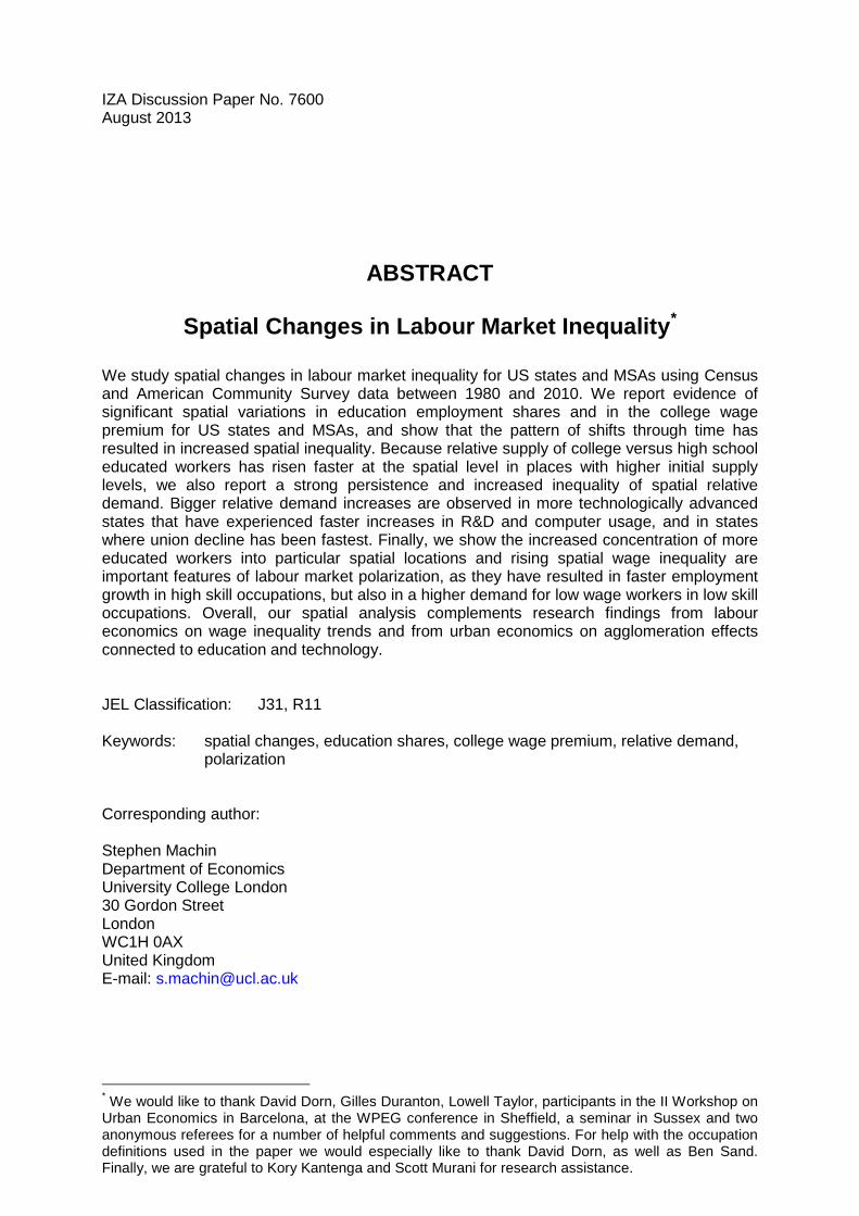
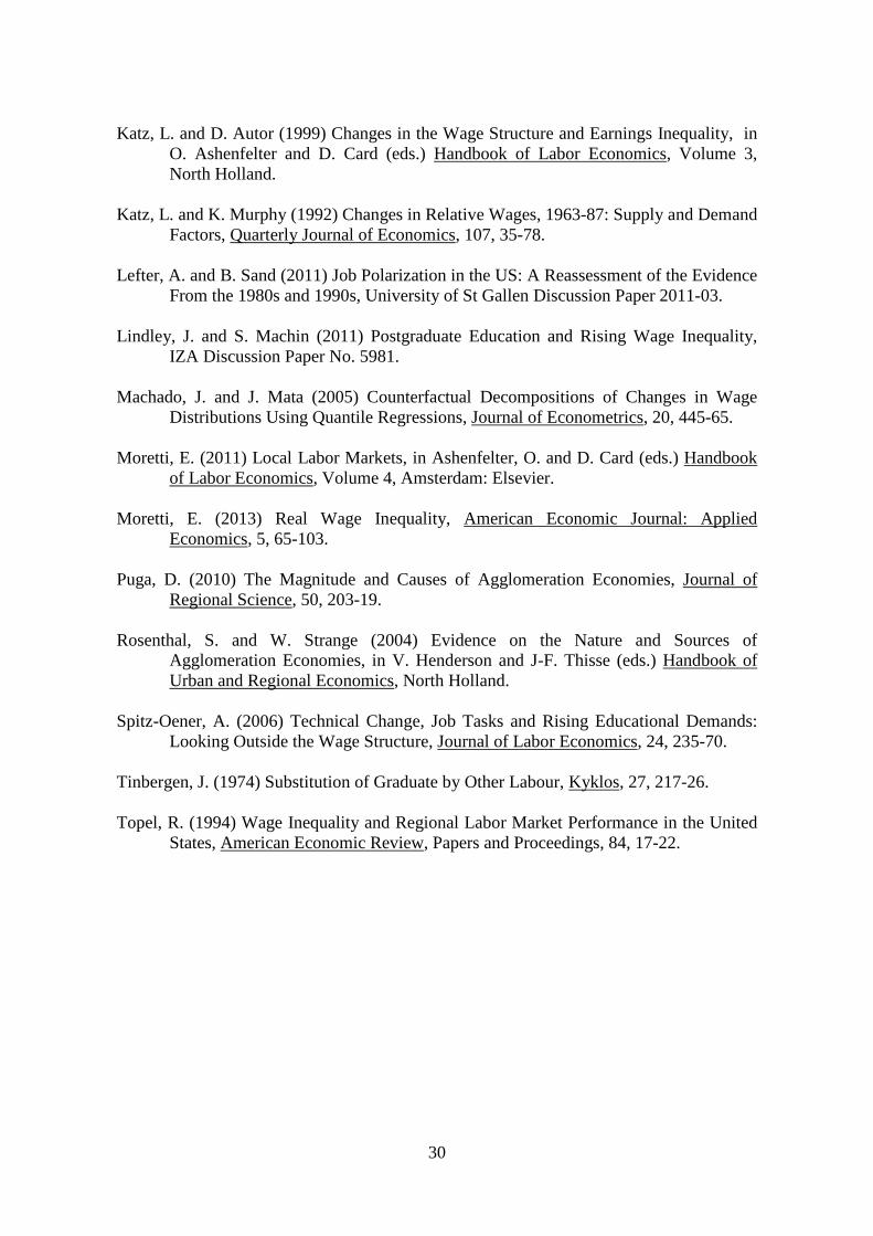
higher wage growth in places with higher initial wages. Moretti (2011), for example,

shows plots of the wages of college graduates and high school graduates in 288 US

Metropolitan Statistical Areas (MSAs) in 1980 and 2000 where wages grow faster in

MSAs with higher wage levels in 1980 for both groups of workers. We find a similar

pattern using data between 1980 and 2010 for 216 MSAs, as shown in Figure 1.5 This

shows either constant or faster increases, and no evidence of convergence, in wage levels

in MSAs with higher wage levels in 1980. For college workers there is significantly higher

wage growth in MSAs where their wages were already higher in 1980.

In this paper, our interest is in the spatial dimensions of labour market inequality

and how they have altered through time. We study changing patterns of spatial college

wage premia in the context of changing relative supply and demand of college educated

versus high school educated workers. In a similar vein to some of the aspects of earlier

work by Berry and Glaeser (2005), Black, Kolesnikova and Taylor (2009) and Moretti

(2013), we begin by documenting the nature of changes in education-specific employment

shares and the college wage premium across different spatial units, looking at their

4 See, inter alia, Barro and Sala-i-Martin (1991) who show regional income convergence using data from the mid-1800s up to 1980. 5 The Figure is based on the 5 percent 1980, 1990 and 2000 Censuses and the 1 percent samples of the 2009, 2010 and 2011 ACS which we collapse to 216 consistently defined MSAs. The Figure replicates Moretti's (2011) Figure based on 1980 and 2000 Census data. Moretti (2011) reported slope coefficients (and associated standard errors) of 1.82 (0.89) for high school graduates and 3.54 (0.11) for college graduates.

3

evolution over time at state and MSA level. To do so, we use US Census and American

Community Survey (ACS) data from 1980 through 2010 (2009 to 2011 pooled). We

uncover an interesting spatial dimension where, despite very rapid increases in the supply

of college workers, the college wage premia has risen almost everywhere, but to varying

degrees as the spatial variation in the wage gap between college educated and high school

educated workers has become more persistent over time.

In the wage inequality literature, rising wage gaps between college and high school

workers have been connected to shifts in the relative demand and supply of these groups

of workers. Indeed, aggregate evidence shows that a key aspect of rising wage college

premia has been an increased relative demand for college educated workers (see Katz and

Murphy, 1992; Katz and Autor, 1999; Acemoglu and Autor, 2010). The presence of rising

spatial college wage premia at different rates in the face of rapidly rising supply also

suggests there may be differential relative demand shifts occurring at the spatial level. We

thus modify the commonly used relative demand and supply model to calculate the extent

of spatial relative demand shifts and examine variations in their evolution through time.

We also consider what factors may have been correlated with the observed spatial shifts in

relative demand, exploring the extent to which technology measures (like R&D spending,

patent intensity or computer usage) and the reduced importance of labour market

institutions (through union decline) display spatial correlations with changes in relative

demand.

Another key feature of labour market inequality that has featured prominently in

more recent research is the polarization of work across more and less skilled occupations.

Autor, Katz and Kearney (2008) and Autor and Dorn (2013) show that job growth in the

4

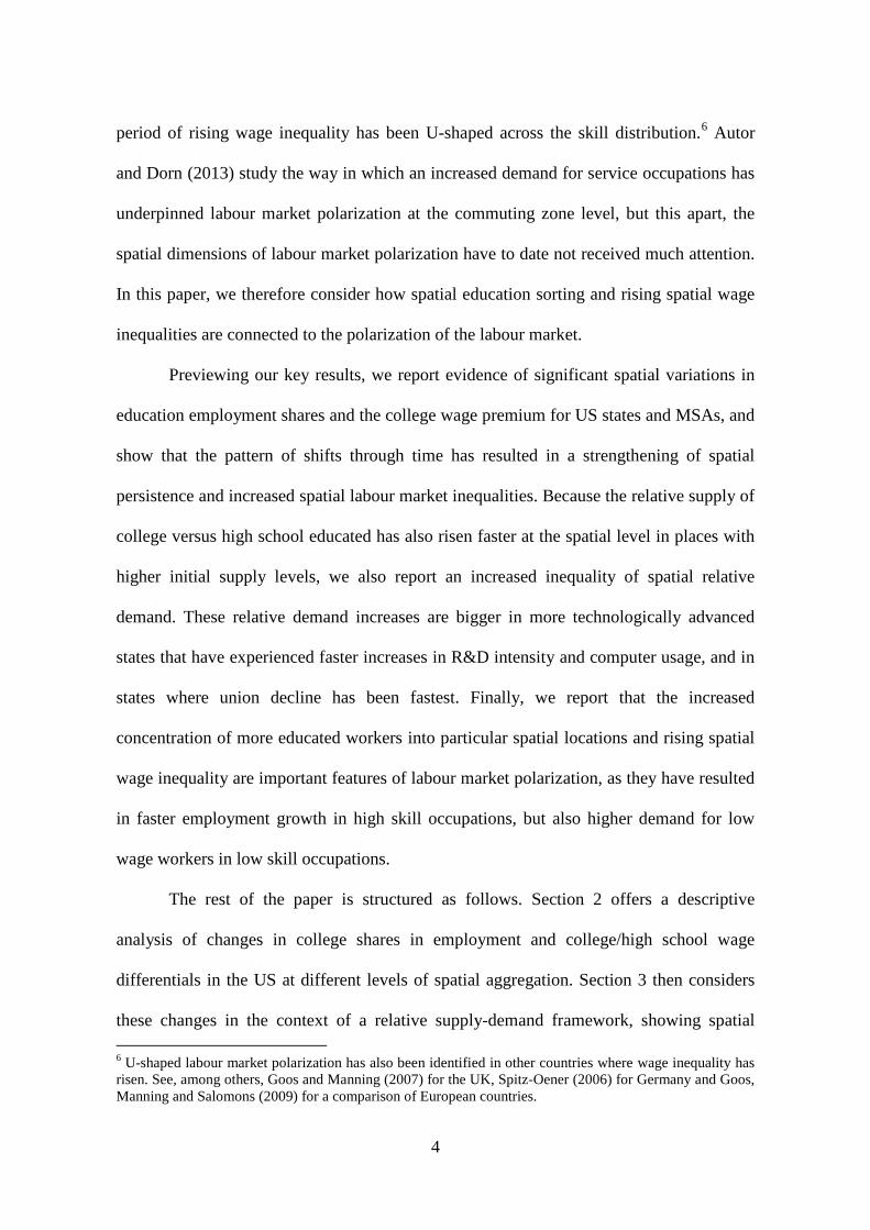
period of rising wage inequality has been U-shaped across the skill distribution.6 Autor

and Dorn (2013) study the way in which an increased demand for service occupations has

underpinned labour market polarization at the commuting zone level, but this apart, the

spatial dimensions of labour market polarization have to date not received much attention.

In this paper, we therefore consider how spatial education sorting and rising spatial wage

inequalities are connected to the polarization of the labour market.

Previewing our key results, we report evidence of significant spatial variations in

education employment shares and the college wage premium for US states and MSAs, and

show that the pattern of shifts through time has resulted in a strengthening of spatial

persistence and increased spatial labour market inequalities. Because the relative supply of

college versus high school educated has also risen faster at the spatial level in places with

higher initial supply levels, we also report an increased inequality of spatial relative

demand. These relative demand increases are bigger in more technologically advanced

states that have experienced faster increases in R&D intensity and computer usage, and in

states where union decline has been fastest. Finally, we report that the increased

concentration of more educated workers into particular spatial locations and rising spatial

wage inequality are important features of labour market polarization, as they have resulted

in faster employment growth in high skill occupations, but also higher demand for low

wage workers in low skill occupations.

The rest of the paper is structured as follows. Section 2 offers a descriptive

analysis of changes in college shares in employment and college/high school wage

differentials in the US at different levels of spatial aggregation. Section 3 then considers

these changes in the context of a relative supply-demand framework, showing spatial 6 U-shaped labour market polarization has also been identified in other countries where wage inequality has risen. See, among others, Goos and Manning (2007) for the UK, Spitz-Oener (2006) for Germany and Goos, Manning and Salomons (2009) for a comparison of European countries.

5

variations in the nature of relative demand shifts over time. Section 4 considers the

relationship between state level relative demand shifts and potential correlates of these

shifts. Section 5 considers the spatial dimensions of labour market polarization, whilst

Section 6 concludes.

2. Spatial Employment Shares and Wage Differentials – Initial Descriptive Analysis

To investigate spatial changes in labour market inequality we use data from the US

Census in 1980, 1990 and 2000, and the American Community Survey (ACS) pooled

across 2009 to 2011. We use the 5 percent Census samples and the three 1 percent ACS

samples of 2009, 2010 and 2011 to study the evolution of education employment shares

and wage differentials for the 48 contiguous US states (dropping Alaska, Hawaii and the

District of Columbia) and for 216 consistently defined MSAs. In this analysis, we focus

on US born individuals aged 26-50.7

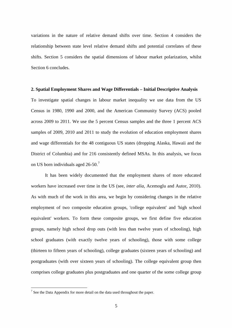
It has been widely documented that the employment shares of more educated

workers have increased over time in the US (see, inter alia, Acemoglu and Autor, 2010).

As with much of the work in this area, we begin by considering changes in the relative

employment of two composite education groups, 'college equivalent' and 'high school

equivalent' workers. To form these composite groups, we first define five education

groups, namely high school drop outs (with less than twelve years of schooling), high

school graduates (with exactly twelve years of schooling), those with some college

(thirteen to fifteen years of schooling), college graduates (sixteen years of schooling) and

postgraduates (with over sixteen years of schooling). The college equivalent group then

comprises college graduates plus postgraduates and one quarter of the some college group

7 See the Data Appendix for more detail on the data used throughout the paper.

6

(both weighted by their wage relative to college graduates).8 High school equivalent

workers are defined analogously as high school graduates or high school dropouts plus

three quarters of some college workers (with the high school dropouts and some college

workers having efficiency weights defined as their wage relative to high school

graduates).

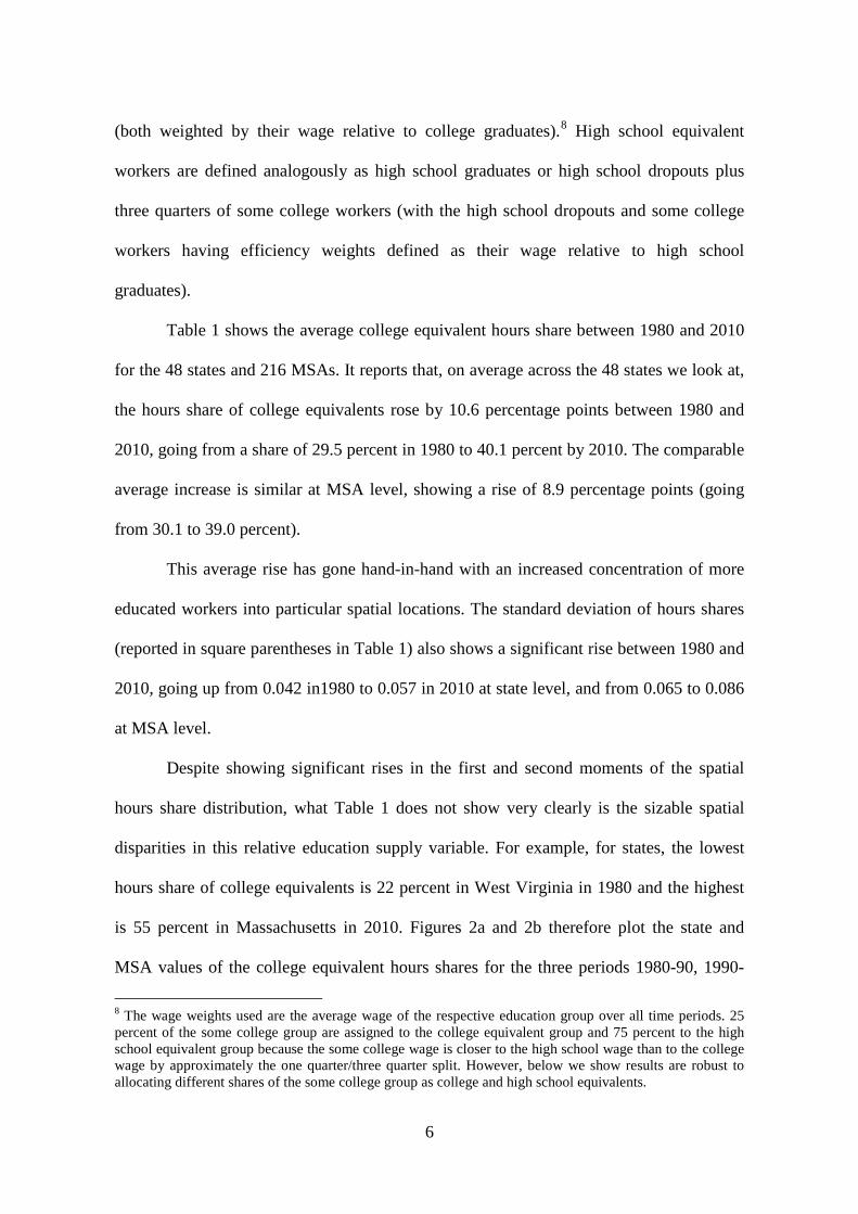
Table 1 shows the average college equivalent hours share between 1980 and 2010

for the 48 states and 216 MSAs. It reports that, on average across the 48 states we look at,

the hours share of college equivalents rose by 10.6 percentage points between 1980 and

2010, going from a share of 29.5 percent in 1980 to 40.1 percent by 2010. The comparable

average increase is similar at MSA level, showing a rise of 8.9 percentage points (going

from 30.1 to 39.0 percent).

This average rise has gone hand-in-hand with an increased concentration of more

educated workers into particular spatial locations. The standard deviation of hours shares

(reported in square parentheses in Table 1) also shows a significant rise between 1980 and

2010, going up from 0.042 in1980 to 0.057 in 2010 at state level, and from 0.065 to 0.086

at MSA level.

Despite showing significant rises in the first and second moments of the spatial

hours share distribution, what Table 1 does not show very clearly is the sizable spatial

disparities in this relative education supply variable. For example, for states, the lowest

hours share of college equivalents is 22 percent in West Virginia in 1980 and the highest

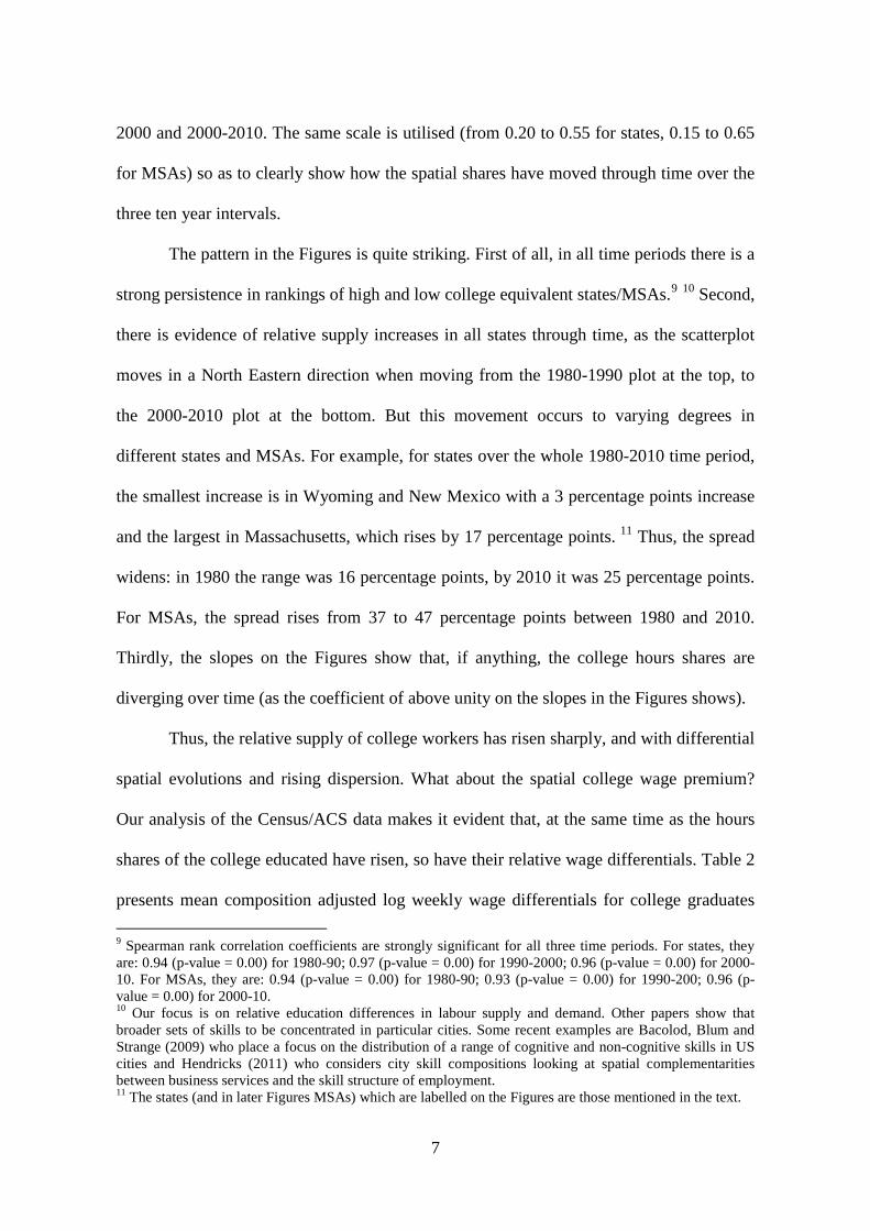
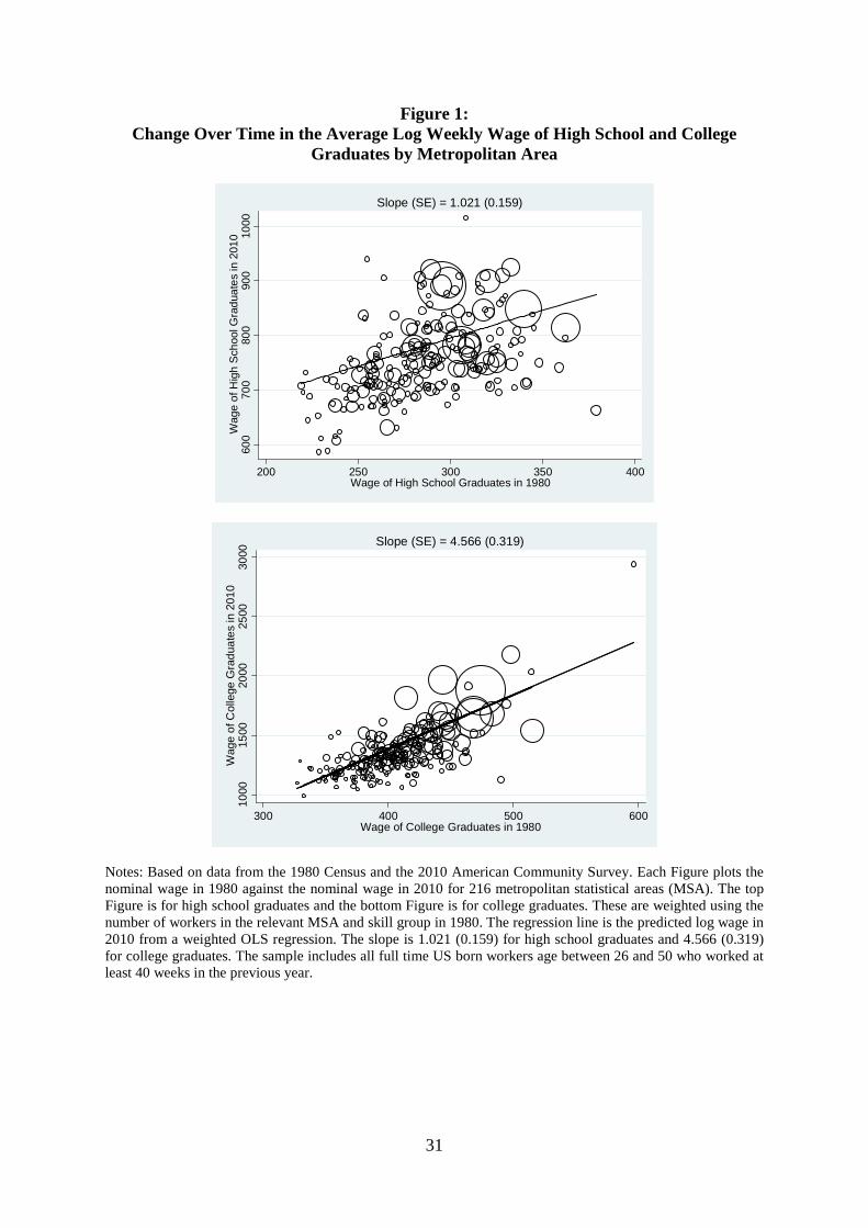
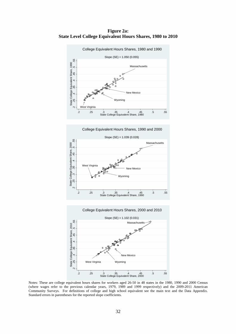
is 55 percent in Massachusetts in 2010. Figures 2a and 2b therefore plot the state and

MSA values of the college equivalent hours shares for the three periods 1980-90, 1990-

8 The wage weights used are the average wage of the respective education group over all time periods. 25 percent of the some college group are assigned to the college equivalent group and 75 percent to the high school equivalent group because the some college wage is closer to the high school wage than to the college wage by approximately the one quarter/three quarter split. However, below we show results are robust to allocating different shares of the some college group as college and high school equivalents.

7

2000 and 2000-2010. The same scale is utilised (from 0.20 to 0.55 for states, 0.15 to 0.65

for MSAs) so as to clearly show how the spatial shares have moved through time over the

three ten year intervals.

The pattern in the Figures is quite striking. First of all, in all time periods there is a

strong persistence in rankings of high and low college equivalent states/MSAs.9 10 Second,

there is evidence of relative supply increases in all states through time, as the scatterplot

moves in a North Eastern direction when moving from the 1980-1990 plot at the top, to

the 2000-2010 plot at the bottom. But this movement occurs to varying degrees in

different states and MSAs. For example, for states over the whole 1980-2010 time period,

the smallest increase is in Wyoming and New Mexico with a 3 percentage points increase

and the largest in Massachusetts, which rises by 17 percentage points. 11 Thus, the spread

widens: in 1980 the range was 16 percentage points, by 2010 it was 25 percentage points.

For MSAs, the spread rises from 37 to 47 percentage points between 1980 and 2010.

Thirdly, the slopes on the Figures show that, if anything, the college hours shares are

diverging over time (as the coefficient of above unity on the slopes in the Figures shows).

Thus, the relative supply of college workers has risen sharply, and with differential

spatial evolutions and rising dispersion. What about the spatial college wage premium?

Our analysis of the Census/ACS data makes it evident that, at the same time as the hours

shares of the college educated have risen, so have their relative wage differentials. Table 2

presents mean composition adjusted log weekly wage differentials for college graduates 9 Spearman rank correlation coefficients are strongly significant for all three time periods. For states, they are: 0.94 (p-value = 0.00) for 1980-90; 0.97 (p-value = 0.00) for 1990-2000; 0.96 (p-value = 0.00) for 2000-10. For MSAs, they are: 0.94 (p-value = 0.00) for 1980-90; 0.93 (p-value = 0.00) for 1990-200; 0.96 (p-value = 0.00) for 2000-10. 10 Our focus is on relative education differences in labour supply and demand. Other papers show that broader sets of skills to be concentrated in particular cities. Some recent examples are Bacolod, Blum and Strange (2009) who place a focus on the distribution of a range of cognitive and non-cognitive skills in US cities and Hendricks (2011) who considers city skill compositions looking at spatial complementarities between business services and the skill structure of employment. 11 The states (and in later Figures MSAs) which are labelled on the Figures are those mentioned in the text.

8

relative to high school graduates across states and MSAs.12 One can see the well known

average pattern of increasing wage payoffs to college graduates as the college/high school

log wage premium rises by 0.259 percentage points between 1980 and 2010 across states

of residence and by 0.257 percentage points across MSAs. The standard deviation of the

composition adjusted spatial wage differentials also increases over time at state and MSA

level, revealing rising inequality in the spatial college wage premium through time.

Previous research by Black, Kolesnikova and Taylor (2009) has noted that, at a

point in time (in their case the cross-sections from the 1980, 1990 and 2000 US Census),

there are sizable spatial disparities in education related wage differentials. This is also the

case for our analysis, both in terms of the yearly variations across spatial units (thus

confirming the Black, Kolesnikova and Taylor findings) and in terms of the sharp increase

in the college premium and its variability.

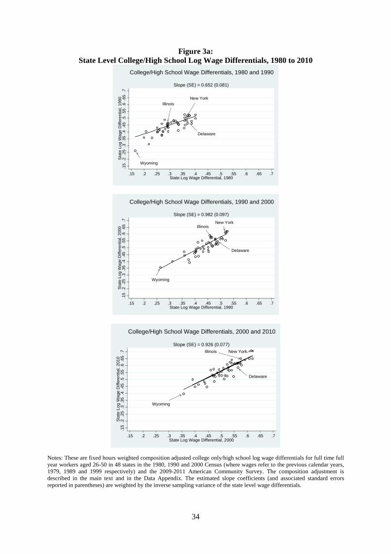
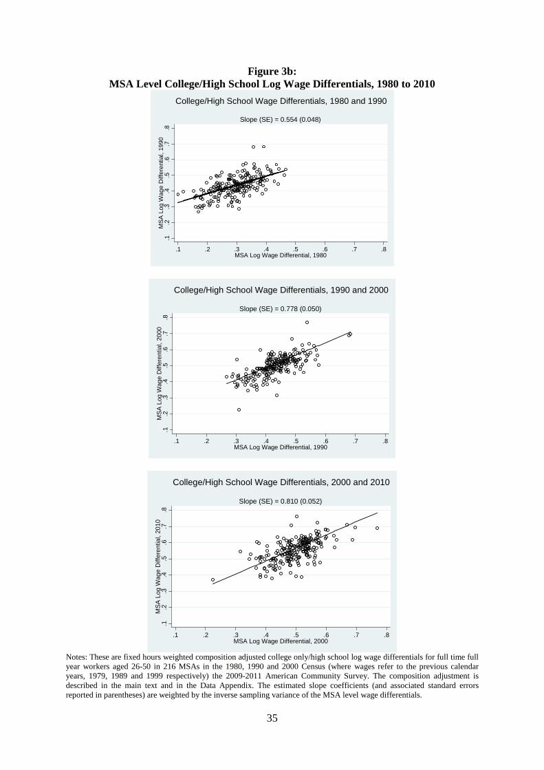
This can also be described in the same way as for our earlier analysis of relative

education supply, as Figures 3a and 3b show the spatial distributions of the college wage

premium for the three sub-periods, 1980-1990, 1990-2000 and 2000-2010. There is very

clear evidence of wide variations in the college premium. The lowest college/high school

wage differential is 0.16 log points in Wyoming in 1980 and the highest is 0.71 log points

in New York in 2010. Within years there is a wide spread which widens over time, from

0.23 log points in 1980, reaching 0.31 log points by 2010. Comparing the three Panels in

12 To ensure that we study movement in spatial wage premia that are likely to be related to productivity changes rather than changes in composition, the wages are composition adjusted on the basis of estimating log weekly wage equations for full time full year workers separately for each year, for five sets of five year birth cohorts/ages and by gender in each year for the 48 states and 216 MSAs respectively. The equations include dummies for age and race. To derive the composition adjusted educational wage differentials, education dummies are included for college workers (comprising postgraduates with more than 16 years of education and college only workers with 16 years of education), some college (13 to 15 years of education) and high school dropouts (less than 12 years of education) relative to the omitted group of high school graduates (12 years of schooling). The college/high school graduate log wage differential is the estimated coefficient on the college variable, which we weight across the sub-groups for states/MSAs over the 1980 to 2010 time period.

9

the Figures also reveals, as was the case for relative supply changes, a significant North

Eastern movement over time. Thus, the college wage premium rises in all states, mirroring

the national pattern, but it goes up by more in some places. In terms of states, the smallest

rise is in Delaware (at 0.15 log points) and the largest is in Illinois (at 0.36 log points).

This upward movement in spatial wage differentials is also characterised by

persistence over time, and a persistence that seems to get stronger. For the state level

analysis in Figure 3a, the estimated slope over the ten year interval rises from 0.65 in

1980-1990 to 0.93 in 1990-2010 and 0.93 in 2000-2010. Thus, in the first decade there is

some evidence of catch up, or mean reversion in the wage premia, from the states that has

lower wage premia to begin with. However, this alters in 1990-2000 and 2000-2010 where

the slope steepens as the premia move in the North Eastern direction in the Figures and

become insignificantly different from unity. The same qualitative pattern of a steepening

slope also occurs in the MSA data in Figure 3b, although there is also more evidence of

mean reversion at this more disaggregated level (possibly due to more noise because of

smaller samples of individuals from the Census/ACS data at this level of aggregation).

This descriptive section of the paper has highlighted spatial disparities in education

supply and in the college wage premium in the US over the last thirty years. In the

remainder of the paper, we focus on reasons why these disparities are present and why

they have been persistent. In the next section we consider spatial demand and supply

models that enable us to use these patterns of change in education supply and the college

wage premium to calculate spatial shifts in relative demand.

10

3. Spatial Relative Supply and Demand Models

The spatial dimensions of rising supply of more educated workers and simultaneously

rising college wage premia suggests a need to consider how these empirical phenomena

map into a supply-demand model of spatial labour markets. Consequently, we now draw

upon the Katz and Murphy (1992) canonical model of relative supply and demand to see if

there are differential relative demand shifts by state and MSA.

The starting point is a Constant Elasticity of Substitution production function

where output in for state or MSA s in period t (Yst) is produced by two education groups

(E1st and E2st) with associated technical efficiency parameters (θ1st and θ2st) as follows:

1/ρρ2st2st

ρ1st1stst )EθE(θY += (1)

where ρ = 1 – 1/σE, and σE is the elasticity of substitution between the two education

groups.

Equating wages to marginal products for each education group, taking logs and

expressing as a ratio leads to a relative wage equation (or inverse relative demand

function) of the form

=

2st

1stst

E2st

1st

EE

log- Dσ1

WW

log (2)

where stD is an index of relative demand.13

This equation therefore relates the relative wage to relative demand and supply

factors, and this is why the approach is sometimes framed as a race between supply and

demand.14 The extent to which increases in relative supply affect relative wages is

determined by the elasticity of substitution between the education groups of interest, σE. A

13 For the production function in (1), Dst = log(θ1st/θ2st). 14 This dates back to Tinbergen (1974).

11

by now quite large literature has, in various ways, attempted to estimate σE.15 For our

purposes, we would like an estimate of σE at the spatial level, so that we can construct a

measure of implied relative demand at the spatial level by rearranging equation (2) as:

WW

logEσ EE

log stD2st

1st

2st

1st

+

= (3)

where spatial relative demand is the relative supply plus the product of the elasticity of

substitution and the relative wage.

There are two main routes to obtaining an estimate of σE which we can use to put

together the patterns of spatial college wage premia and spatial relative education supplies

we described in Section 2 of the paper to form this index of spatial relative demand. First,

we could use estimates from existing research. However, there are only a few at state

level as most existing estimates are at the aggregate level. Moreover, the ones that do exist

do not match our samples and time period of study. Thus, we decided to follow the second

route and estimate σE ourselves. To check robustness, we do also benchmark our estimates

to other state level estimates of the substitution elasticity (albeit from the different samples

studied in Ciccone and Peri, 2005, and Fortin, 2006). It is worth noting that this is not at

all fundamental for our analysis as we are only going to use a single estimate of σE applied

to all states and so it is really only a scaling factor that weights the relative employment

and wage parts of the demand shift. Nonetheless, we do require an estimate to calculate

the implied relative demand shifts and so use an estimate from our own empirical analysis

and also calibrate using an upper and lower bound from the existing literature.

An issue in estimating σE, particularly at the sub-national level, is the possibility of

bias emerging from geographical migration or because of potential endogeneity. In

15 For the traditional labour demand work, see Hamermesh (1993). For the wage inequality research, see Acemoglu and Autor (2010).

12

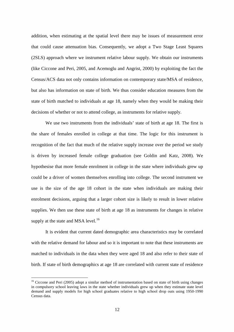
addition, when estimating at the spatial level there may be issues of measurement error

that could cause attenuation bias. Consequently, we adopt a Two Stage Least Squares

(2SLS) approach where we instrument relative labour supply. We obtain our instruments

(like Ciccone and Peri, 2005, and Acemoglu and Angrist, 2000) by exploiting the fact the

Census/ACS data not only contains information on contemporary state/MSA of residence,

but also has information on state of birth. We thus consider education measures from the

state of birth matched to individuals at age 18, namely when they would be making their

decisions of whether or not to attend college, as instruments for relative supply.

We use two instruments from the individuals’ state of birth at age 18. The first is

the share of females enrolled in college at that time. The logic for this instrument is

recognition of the fact that much of the relative supply increase over the period we study

is driven by increased female college graduation (see Goldin and Katz, 2008). We

hypothesise that more female enrolment in college in the state where individuals grew up

could be a driver of women themselves enrolling into college. The second instrument we

use is the size of the age 18 cohort in the state when individuals are making their

enrolment decisions, arguing that a larger cohort size is likely to result in lower relative

supplies. We then use these state of birth at age 18 as instruments for changes in relative

supply at the state and MSA level.16

It is evident that current dated demographic area characteristics may be correlated

with the relative demand for labour and so it is important to note that these instruments are

matched to individuals in the data when they were aged 18 and also refer to their state of

birth. If state of birth demographics at age 18 are correlated with current state of residence

16 Ciccone and Peri (2005) adopt a similar method of instrumentation based on state of birth using changes in compulsory school leaving laws in the state whether individuals grew up when they estimate state level demand and supply models for high school graduates relative to high school drop outs using 1950-1990 Census data.

13

demographics then this may raise concerns about the suitability of this identification

strategy. The extent to which this is the case therefore adds extra justification for

considering alternative estimates of σE that come from other identification strategies used

in the related literature.

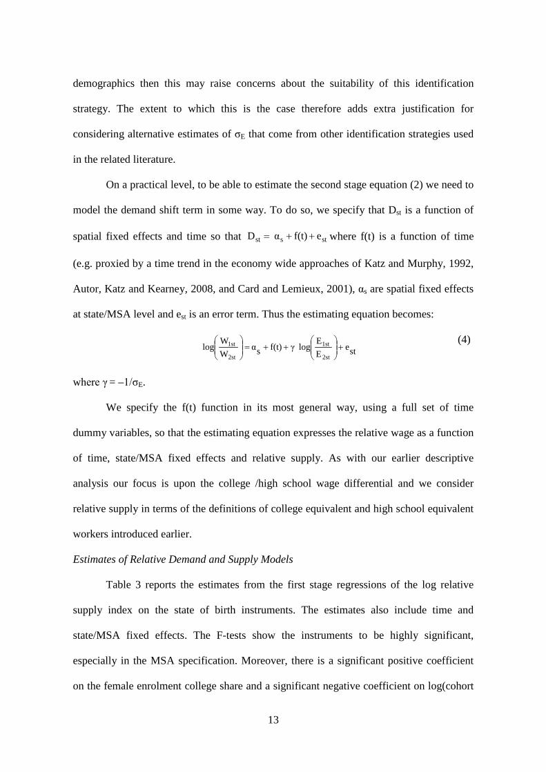
On a practical level, to be able to estimate the second stage equation (2) we need to

model the demand shift term in some way. To do so, we specify that Dst is a function of

spatial fixed effects and time so that stsst ef(t)α D ++= where f(t) is a function of time

(e.g. proxied by a time trend in the economy wide approaches of Katz and Murphy, 1992,

Autor, Katz and Kearney, 2008, and Card and Lemieux, 2001), αs are spatial fixed effects

at state/MSA level and est is an error term. Thus the estimating equation becomes:

steEE

log γ f(t) sα WW

log2st

1st

2st

1st +

++=

(4)

where γ = –1/σE.

We specify the f(t) function in its most general way, using a full set of time

dummy variables, so that the estimating equation expresses the relative wage as a function

of time, state/MSA fixed effects and relative supply. As with our earlier descriptive

analysis our focus is upon the college /high school wage differential and we consider

relative supply in terms of the definitions of college equivalent and high school equivalent

workers introduced earlier.

Estimates of Relative Demand and Supply Models

Table 3 reports the estimates from the first stage regressions of the log relative

supply index on the state of birth instruments. The estimates also include time and

state/MSA fixed effects. The F-tests show the instruments to be highly significant,

especially in the MSA specification. Moreover, there is a significant positive coefficient

on the female enrolment college share and a significant negative coefficient on log(cohort

14

size). Thus these instruments seem to work well, and in the empirical direction as

hypothesised above.

Table 4 provides the 2SLS estimates of equation (4). Again, these include time and

geographical fixed effects. The estimate of the labour supply parameter γ is negative, and

quite precisely determined, for the state and MSA models. At state level, the 2SLS

estimate is -0.489, which provides an estimated elasticity of substitution of 2.05. For the

MSA level estimates, the estimate of γ equal to -0.340 is smaller (in absolute magnitude)

with an estimated elasticity of substitution of 2.94.17 18 These magnitudes are in line with

estimates in the aggregate literature: for example, Lindley and Machin (2011) derive an

estimate of around 2.6 using aggregate March CPS data from 1963 to 2010 which is in the

same ballpark as Autor, Katz and Kearney's (2008) estimate of 2.4, who also analyse the

same March CPS data with a time series of five fewer years (from 1963 to 2005).19

The estimated parameters on the time dummies in Table 4 also tell us something

about the relative demand shifts that have occurred on a decade by decade basis. Relative

to the 1980s the relative demand for college graduates has increased across all time

periods although these incremental changes get smaller over time. This is in line with

there being a quadratic relationship over the thirty years we study, or a slowing down of

17 We also restricted the college wage premium to include just college only workers (excluding postgraduates). Doing so produced an estimate (standard error) of γ = -0.452 (0.168) at the state level, with an elasticity of substitution of 2.21. At the MSA level the estimate was -0.359 (0.103), generating an elasticity of 2.79. 18 Restricting the college equivalent labour supply to include only college plus and postgraduate workers, by placing all (rather than 75 percent) of some college workers into the high school equivalent group produced estimates (and standard errors) of γ = -0.441 (0.158) at the state level and -0.315 (0.090) at the MSA level. Allocating half of some college workers to each group produced state and MSA estimates of -0.513 (0.212) and -0.368 (0.109) respectively. 19 Like Ciccone and Peri (2005) we also considered other estimation methods that are robust to issues to do with potentially weak instruments. Our instruments do not seem to suffer from such an issue (see the F-statistics reported in Table 3), but we also used limited information maximum likelihood (LIML) estimation methods to produce very similar estimates. For example, the state level 2SLS estimate (and standard error) of γ = -0.489 (0.186) was numerically the same.

15

the increased relative wage in the 2000s (as also noted in Beaudry, Green and Sand, 2013,

in the aggregate).20

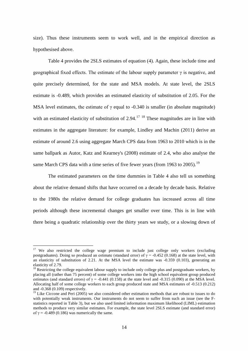
Implied Relative Demand Shifts

We are now in a position to combine the spatial changes in wage differentials and

supply into an implied relative demand index using our estimates of σE. As noted above,

the demand index for spatial unit s in year t can be calculated as

)/Wlog(Wσ )/Elog(E D 2st1stE2st1stst += for any two particular education groups. We

construct the spatial relative demand index based upon our relative supply measure of

college equivalent (CE) versus high school equivalent (HE) workers and our composition

adjusted college/high school wage differentials (WC/WH) as

)/Wlog(Wσ )/Elog(E D Hst

CstE

HEst

CEstst += .

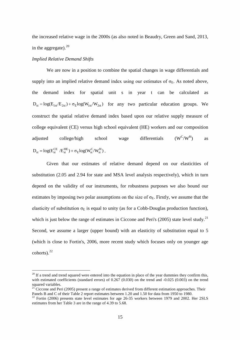
Given that our estimates of relative demand depend on our elasticities of

substitution (2.05 and 2.94 for state and MSA level analysis respectively), which in turn

depend on the validity of our instruments, for robustness purposes we also bound our

estimates by imposing two polar assumptions on the size of σE. Firstly, we assume that the

elasticity of substitution σE is equal to unity (as for a Cobb-Douglas production function),

which is just below the range of estimates in Ciccone and Peri's (2005) state level study.21

Second, we assume a larger (upper bound) with an elasticity of substitution equal to 5

(which is close to Fortin's, 2006, more recent study which focuses only on younger age

cohorts).22

20 If a trend and trend squared were entered into the equation in place of the year dummies they confirm this, with estimated coefficients (standard errors) of 0.267 (0.030) on the trend and -0.025 (0.003) on the trend squared variables. 21 Ciccone and Peri (2005) present a range of estimates derived from different estimation approaches. Their Panels B and C of their Table 2 report estimates between 1.20 and 1.50 for data from 1950 to 1980. 22 Fortin (2006) presents state level estimates for age 26-35 workers between 1979 and 2002. Her 2SLS estimates from her Table 3 are in the range of 4.39 to 5.68.

16

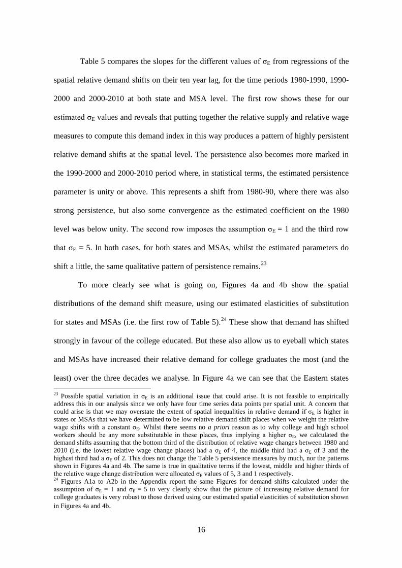
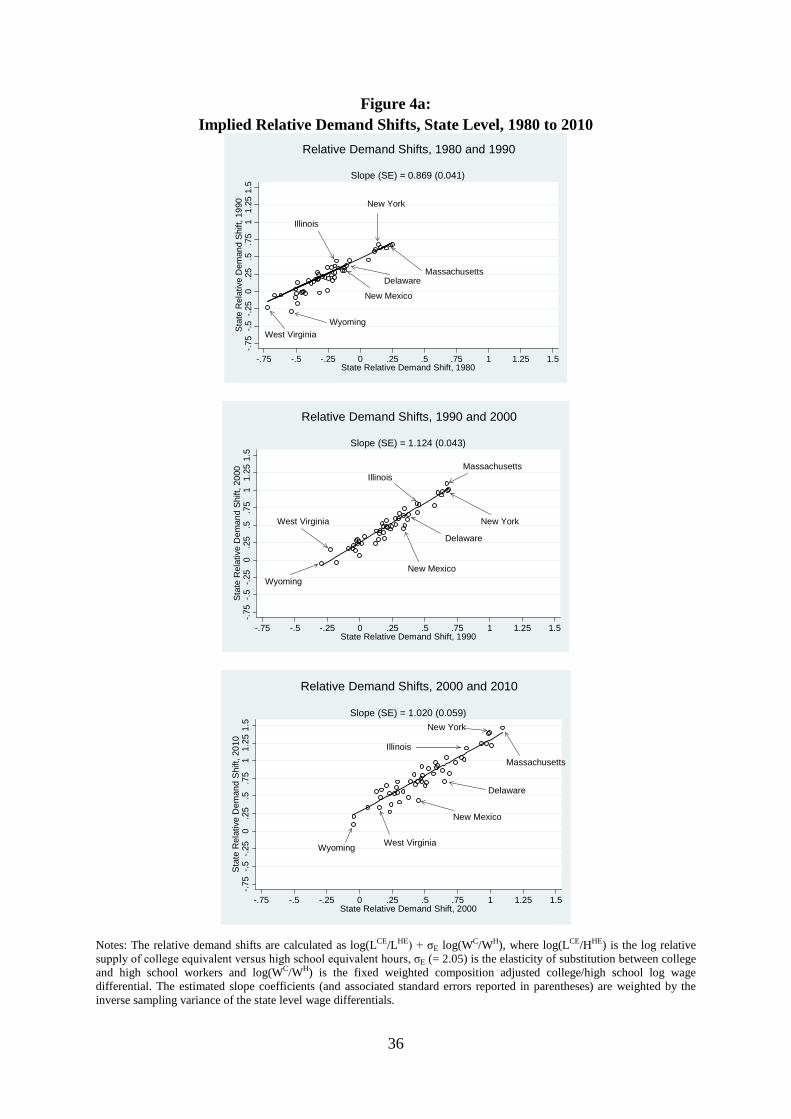
Table 5 compares the slopes for the different values of σE from regressions of the

spatial relative demand shifts on their ten year lag, for the time periods 1980-1990, 1990-

2000 and 2000-2010 at both state and MSA level. The first row shows these for our

estimated σE values and reveals that putting together the relative supply and relative wage

measures to compute this demand index in this way produces a pattern of highly persistent

relative demand shifts at the spatial level. The persistence also becomes more marked in

the 1990-2000 and 2000-2010 period where, in statistical terms, the estimated persistence

parameter is unity or above. This represents a shift from 1980-90, where there was also

strong persistence, but also some convergence as the estimated coefficient on the 1980

level was below unity. The second row imposes the assumption σE = 1 and the third row

that σE = 5. In both cases, for both states and MSAs, whilst the estimated parameters do

shift a little, the same qualitative pattern of persistence remains.23

To more clearly see what is going on, Figures 4a and 4b show the spatial

distributions of the demand shift measure, using our estimated elasticities of substitution

for states and MSAs (i.e. the first row of Table 5).24 These show that demand has shifted

strongly in favour of the college educated. But these also allow us to eyeball which states

and MSAs have increased their relative demand for college graduates the most (and the

least) over the three decades we analyse. In Figure 4a we can see that the Eastern states 23 Possible spatial variation in σE is an additional issue that could arise. It is not feasible to empirically address this in our analysis since we only have four time series data points per spatial unit. A concern that could arise is that we may overstate the extent of spatial inequalities in relative demand if σE is higher in states or MSAs that we have determined to be low relative demand shift places when we weight the relative wage shifts with a constant σE. Whilst there seems no a priori reason as to why college and high school workers should be any more substitutable in these places, thus implying a higher σE, we calculated the demand shifts assuming that the bottom third of the distribution of relative wage changes between 1980 and 2010 (i.e. the lowest relative wage change places) had a σE of 4, the middle third had a σE of 3 and the highest third had a σE of 2. This does not change the Table 5 persistence measures by much, nor the patterns shown in Figures 4a and 4b. The same is true in qualitative terms if the lowest, middle and higher thirds of the relative wage change distribution were allocated σE values of 5, 3 and 1 respectively. 24 Figures A1a to A2b in the Appendix report the same Figures for demand shifts calculated under the assumption of σE = 1 and σE = 5 to very clearly show that the picture of increasing relative demand for college graduates is very robust to those derived using our estimated spatial elasticities of substitution shown in Figures 4a and 4b.

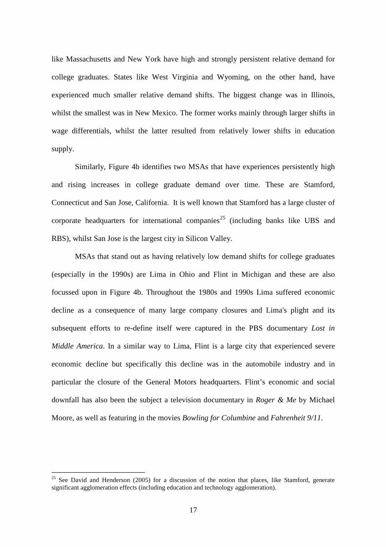
17

like Massachusetts and New York have high and strongly persistent relative demand for

college graduates. States like West Virginia and Wyoming, on the other hand, have

experienced much smaller relative demand shifts. The biggest change was in Illinois,

whilst the smallest was in New Mexico. The former works mainly through larger shifts in

wage differentials, whilst the latter resulted from relatively lower shifts in education

supply.

Similarly, Figure 4b identifies two MSAs that have experiences persistently high

and rising increases in college graduate demand over time. These are Stamford,

Connecticut and San Jose, California. It is well known that Stamford has a large cluster of

corporate headquarters for international companies25 (including banks like UBS and

RBS), whilst San Jose is the largest city in Silicon Valley.

MSAs that stand out as having relatively low demand shifts for college graduates

(especially in the 1990s) are Lima in Ohio and Flint in Michigan and these are also

focussed upon in Figure 4b. Throughout the 1980s and 1990s Lima suffered economic

decline as a consequence of many large company closures and Lima's plight and its

subsequent efforts to re-define itself were captured in the PBS documentary Lost in

Middle America. In a similar way to Lima, Flint is a large city that experienced severe

economic decline but specifically this decline was in the automobile industry and in

particular the closure of the General Motors headquarters. Flint’s economic and social

downfall has also been the subject a television documentary in Roger & Me by Michael

Moore, as well as featuring in the movies Bowling for Columbine and Fahrenheit 9/11.

25 See David and Henderson (2005) for a discussion of the notion that places, like Stamford, generate significant agglomeration effects (including education and technology agglomeration).

http://en.wikipedia.org/wiki/PBS

http://en.wikipedia.org/w/index.php?title=Lost_in_Middle_America&action=edit&redlink=1

http://en.wikipedia.org/w/index.php?title=Lost_in_Middle_America&action=edit&redlink=1

http://en.wikipedia.org/wiki/Roger_%26_Me

http://en.wikipedia.org/wiki/Michael_Moore

http://en.wikipedia.org/wiki/Michael_Moore

http://en.wikipedia.org/wiki/Bowling_for_Columbine

http://en.wikipedia.org/wiki/Fahrenheit_9/11

18

4. Correlates of Spatial Relative Demand Shifts

We can relate our estimated spatial relative demand shifts to variables that can be directly

measured at the state level. We have looked at four different potential factors at state level

that have been considered in some of the existing literature, but which are usually

analysed at the aggregate or industry level.26 These are changes in the R&D stock

(measured relative to state GDP), patent intensities (measured by the number of new

patents per worker) and the proportions of workers using computers and who are covered

by union collective bargaining.27

Our empirical model studies how decadal spatial changes in relative demand relate

to these variables in a framework where we also allow for the spatial persistence in

relative demand seen in the spatial auto-regressions reported in Table 5 above. We do so

by including the lag of the spatial relative demand index in the estimated change

equations, allowing for differential persistence by decade via time varying coefficients.

The estimating equation is:

stυ tTstλΔZ)tT x 3

1d10ts,(Ddδ stΔD +++∑

=−= (5)

where Z denotes the potential correlates of relative demand we consider, T is a set of year

dummies and υ an error term and we estimate the model on the three decadal changes (d =

1 to 3, corresponding to 1980-1990, 1990-2000 and 2000-2010).

26 Like the aggregate and industry level studies, we also study associations between these factors and changing relative demand at the spatial level in a descriptive manner to explore correlations. Generally this is an area where finding credible instruments for a causal analysis is demanding. 27 We include computer use alongside our other technology measures with an acknowledgment that Beaudry, Doms and Lewis (2010) critically appraise the extent to which the widespread use of personal computers reflects a technological revolution, especially as in the recent past computers have very much become a general purpose technology.

19

Table 6 reports estimates of equation (5).28 The first four columns shows estimates

when we entered the four Z variables of interest separately and the fifth when we enter

them all at the same time into a change in demand equation where D is calculated using

our estimated spatial elasticities of substitution. The final two columns show estimates

with all Z variables simultaneously included when we assume our two polar extremes for

an elasticity of substitution equal to 1 and 5.

When entered separately into the equation, the Z variables mostly display a

significant association with changes in relative demand at the state level. Over the thirty

year period we study, increases in relative demand were faster in states with higher R&D

intensities and where more workers use computers (although not with the number of new

patents issued, the coefficient on which is positive but insignificant). Thus technology

improvements related to R&D and computers have gone hand-in-hand with increases in

relative demand. At the same time, states where collective bargaining coverage has fallen

by more have also seen slower demand shifts in favour of more educated workers. When

entered simultaneously (as reported in column (5) of Table 6), the same pattern remains,

revealing that the positive association with faster technological changes, and with faster

union decline, remain robust to allowing for them all to have a role.

In the final two columns of the Table, we consider models of changes in relative

demand for the alternative assumptions of the value of the elasticity of substitution

between college and high school graduates. The same overall pattern of results remains,

but there are some more nuanced shifts in the associations between changes in relative

28 Note that the estimates are weighted by the inverse sampling variance of the state level wage differentials since the wage differentials are themselves estimates.

20

demand and technology and union measures.29 For an elasticity of substitution of unity

(where the demand shift variable becomes the relative wage bill), the computer and R&D

variable dominate the technology associations as the estimated coefficient on the new

patents per worker variable remains insignificantly different from zero. However, for an

assumed elasticity of substitution of five, the patents variable does attract a positive and

significant coefficient. As the difference is a bigger weight on the relative wage term in

computing demand shifts for the larger elasticity, this seems to suggest that the patents and

R&D variables work through a stronger correlation with increased relative wages.

Because the scale of the dependent variable, and therefore also the estimated

coefficients, differ under the σE assumptions it is also useful to consider the magnitudes of

the empirical associations. The standard deviation of the relative demand shifts dependent

variable is 0.461 for columns (1)-(5) of the Table, 0.360 for column (6) and 0.776 for

column (7). We can calculate how much of this a one standard deviation increase in our

four main independent variables can account for.30 In the specifications where all four

variables are entered simultaneously (columns (5)-(7)), the ranges of magnitudes that

emerge from the three specifications are as follows: R&D intensity, 7.8 to 12.4 percent;

Patents, -2.8 to 5.4 percent; Computer usage, 13.6 to 19.6 percent; Union coverage, -21.0

to -12.9 percent.

Figure 5 further shows the spatial aspects of these empirical connections between

the state level relative demand increases and technology/union variables, by plotting long

run 1980-2010 spatial demand shifts against the four potential demand side factors 29 A higher elasticity of substitution places more weight on the relative wage movements as compared to the employment movements. We also estimated separate relative wage and relative employment equations (freeing up the elasticity of substitution), with similar results. These are available from the authors on request. 30 That is, by multiplying the estimated coefficient by a one standard deviation increase in the independent variable of interest and then dividing the resultant product by the standard deviation of the relative demand shifts. So, for example, in column (1) for the R&D variable, which has a standard deviation of 0.070, this is (0.070*0.678) / 0.461 = 0.103, or about 10 percent.

21

connected to inequality. Presenting the empirical associations in graphical form enables us

to see which states are the most and least correlated with the proximate determinants. For

example, Massachusetts has the largest long run increase in R&D, together with a

significant increase in relative demand. The interpretation for identifying the main states

driving the changes in computer use is less obvious, mainly because of the mass

implementation of general purpose computer technology (especially in more recent

decades) which probably makes computers a less good proxy for technical change.

Notice in the plot of the demand shifts against the change in the proportion of

union covered workers there is union decline in all states. This reflects the overall

aggregate longer run decline in union coverage. However, over our sample period, some

of the largest declines occurred in Michigan, Indiana, Pennsylvania, Ohio, Illinois,

Tennessee and West Virginia. These are states that have typically been more affected by

de-industrialisation, with sectoral shifts away from unionised large scale manufacturing

firms and towards non-unionised service sector firms who are also likely to employ more

graduates.

5. Spatial Inequalities and Labour Market Polarization

The increased spatial concentration of more educated workers and rising demand for these

workers has driven up wage inequality, but has also impacted upon the demands for goods

and services on offer in particular spatial locations. Autor and Dorn (2013) have studied

this in detail, arguing that in places where there are now more high paid workers, they

have also increased their demand for services (like child care, or cleaning) that are

typically done by low wage workers. A complementarity between high and low wage

workers (e.g. high wage workers who are now richer wanting a cleaner) has tempered the

22

reduced demand for some low wage occupations, typically those that were not

substitutable by skill-biased technologies. Because of this, the shifts in employment

structure have polarized, with job growth high for high wage occupations that are

complementary to skill-biased technologies, low for low or medium wage occupations that

can be substituted by skill-biased technologies, but with job growth still taking place for

low wage occupations that still have to be done by people and are not substitutable by new

technologies.

This polarization of the labour market is shown in Figure 6. The Figure extends

Autor and Dorn’s analysis to 2010 looking at job growth by skill percentile (defined at the

1980 mean occupational wage across 320 consistently defined occupations) between 1980

and 2010. The job growth is scaled relative to the average across all occupational wage

percentiles and so a positive number shows an increased share in total employment and

negative ones show a decreased share. The pattern is very clear, with very rapid job

growth in the upper part of the distribution, a hollowing out in the middle part (roughly the

20th to 70th percentiles), but increased growth also at the bottom.

What about the spatial level? We carried out the same exercise for our 48 states,

exploring the extent of polarization in state labour markets between 1980 and 2010. This

revealed that almost all state labour markets are characterised by the U-shape polarization

seen for the aggregate labour market in Figure 6. However, there are differences in the

extent of polarization, with some showing a very marked U-shape and others being far

more moderate and some having very little job growth for the lower skill percentiles.

We therefore classified states into three groups (high, medium and low

polarization) so as to show the differential extent of polarization. The three groups’

polarization patterns are presented in Figure 7. The high polarization group (comprising

23

18 states) shows a very marked U-shape, with higher job growth at the top and bottom,

together with a bigger fall in the middle. The medium polarization group (comprising 24

states) displays similarities, but is more muted in growth at the top and bottom, and in the

hollowing out of the middle. The low polarization group (made up of 6 states) shows high

growth at the top, and also loss of middle range jobs, but importantly show no growth at

all in the low wage jobs in the lower percentiles of the distribution.

We can ask the question how much these state-level differences in labour market

polarization are connected to the increased concentration of more educated workers into

particular spatial locations and the rise in wage inequality (measured by the college/high

school wage premium) that we have considered earlier. We do this in two ways. First, we

can consider how spatial education sorting and rising wage inequality have differed across

our classification of high, medium and low polarization states. Second, we can ask the

counterfactual question of what would polarization have looked like in the aggregate had

the state education and inequality changes not occurred (i.e. if they remained at their 1980

levels).

The first consideration is explored in Panel A of Table 7, which shows differences

in the 1980-2010 changes in college equivalent education shares and the college wage

premium across the three groups of states. We know from the earlier analysis that

education sorting and a widening of the college wage gap occurred across all states, but to

varying degrees. The numbers in the table make it evident that the states where there was

more education sorting and where the college wage gap widened the most were the ones

characterised by stronger patterns of polarization.

Our second consideration investigates what the overall polarization Figure would

look like if we held constant the state level education shares and wage differentials at their

24

1980 levels.31 Figure 8 shows these counterfactual experiments. The upper Panel of the

Figure shows that holding constant the extent of education sorting (shown by the dashed

line) strongly dampens down the polarization pattern. A U-shaped polarization pattern

remains, but is much more muted, and of a slightly different shape. At the top end, in

particular, almost all the jobs growth can be accounted for by the spatial education share

changes. The hollowing out of the middle part of the distribution is also explained well by

the changing education shares. At the bottom end of the distribution the changed

education shares play a role, but less than in the other parts of the distribution.

These patterns are consistent with recent discussion in the polarization work which

shows that to uncover a clear U-shaped pattern of labour market polarization, the skill

percentiles on the x-axis of the Figure are better defined in terms of ranks of occupational

wages rather than on occupations ranked by education. If education is used to delineate the

initial skill structure of employment, then less of a U-shape emerges. The likely reason is

that the low wage jobs are not all being done by the lowest education groups and this is in

part why we see the pattern we do in Figure 8 at the bottom part of the distribution.

Overall, however, the Figure shows that spatial education sorting matters as a factor in the

polarization of the labour market.

The lower Panel of Figure 8 shows a counterfactual exercise that holds constant

the college/high school wage differential. This time the shaded counterfactual line shows a

different pattern, explaining very little in the middle and top part of the distribution, but

accounting for most of the change in the lower percentiles. Our interpretation of this is

that spatial differences in the between group wage differential we are considering here is,

31 On a practical level, we carry out this counterfactual exercise in a similar way to the full accounting decompositions of Machado and Mata (2005) or Firpo et al (2010) by standardising job growth in each occupation percentile across states for a variable of interest (the state level change in education shares or the college wage premium) from separate regressions across the 100 percentiles for the 48 states.

25

in this exercise, effectively operating as a barometer of different levels of wage inequality

across states and thus is picking up the notion that the increased demand for low wage

goods and services is higher in higher wage inequality states.

Panel B of Table 7 shows changes in the occupational shares of service jobs and

managerial jobs between 1980 and 2010 (using the classifications of Autor and Dorn,

2013). The high polarization states see a bigger increase in both of these occupational

shares, in line with the notion that increased demand for more educated workers in states

has gone hand-in-hand with an increased demand for low wage services. It is also the case,

again in line with the Autor and Dorn (2013) patterns of change across US commuting

zones, that the places where these occupational shifts were more pronounced were those

where the employment share of occupations involving routine tasks was higher in 1980

(i.e. the kind of jobs which would subsequently be more substitutable by computer capital

or other forms of automation). This is shown for Autor and Dorn’s occupational task

routineness measures in the last row of Panel B of Table 7 which is significantly higher in

the high polarization group of states.32

A final set of observations relates to recent work that considers cost of living

differences between higher and lower inequality locations. Moretti (2013), for example,

reports that house prices are higher and have risen faster in cities where wage inequality

has risen by more. He therefore argues that real wage inequality has risen by less than

nominal wage inequality as the beneficiaries of higher relative wages driven by increased

relative demand have had to pay more on housing costs. Diamond (2012) and Handbury

(2012) also study this question, but by considering wider definitions of well being and

connecting to skill-biased consumption patterns. Diamond argues that the high inequality,

32 As in Autor and Dorn (2013) we define the highest one third of employment weighted occupations based on the share of routine tasks (so by construction the overall mean of the routineness variable is 1/3).

26

high house price locations also have a range of amenities that are demanded by higher

earnings individuals, like more eating and drinking places, or book stores, and grocery and

apparel stores. To the extent that the presence of these amenities drive up the demand for

low wage workers as we have already described, then the polarization patterns we have

found should emerge more in these high inequality, high house price, high amenity places.

Handbury (2012) looks at price differences within cities facing consumers for different

income and skill levels, presenting evidence that income and skill specific consumption

externalities exist.

We have also therefore looked at differences in house prices and amenities for our

high, medium and low polarization states. Table 7 shows significantly higher house price

growth in the high polarization states, and that for the most part there have been bigger

increases in the numbers of eating and drinking places, apparel stores and hair and beauty

salons. This is very much in line with the notion that high polarization locations are

characterised by the sorting in of more educated individuals (who also get paid more) and

that, whilst this has driven up housing costs, to meet their higher standards of living they

have also demanded more services which are supplied by low wage labour. One way of

interpreting this is the presence of skill-biased consumption patterns in places where

labour market polarization has been more pronounced.

6. Concluding Comments

In this paper, we study spatial changes in labour market inequality for states and cities

using US Census and American Community Survey data between 1980 and 2010. We

report evidence of significant spatial variations and increases over time in college

education shares and in the college wage premium for US states and MSAs. We use

27

estimates of spatial relative demand and supply models to calculate implied relative

demand shifts for college graduates vis-à-vis high school graduates. These calculated

demand shifts also show significant spatial disparities that are, if anything, widening over

the time period we study. Considering potential correlates of the differential spatial trends,

we show that relative demand has increased faster in those states and cities that have

experienced faster increases in R&D intensity and computer use, and increased slower in

those states and cities where union decline has been more marked. Finally the extent of

labour market polarization that has occurred is different across states, with more

polarization occurring where there have been bigger increases in college education share

and in spatial wage inequality.

These findings complement those from the more aggregated work in labour

economics on trends in wage inequality, on shifts in the relative demand and supply of

more and less educated workers and on the phenomenon of labour market polarization.

They also complement the work in urban economics that emphasises agglomeration

effects in locations that are strongly connected to education and technology. Our analysis

brings these two strands of research work together, by emphasising that the US has seen

significant rises in educational wage differentials despite rapid increases in education

supply, and that there have been important spatial aspects to this, and to the relative

demand shifts by education and the patterns of labour market polarization that have

occurred over the last thirty years.

28

References

Acemoglu, D. and J. Angrist (2000) How Large are Human-Capital Externalities? Evidence from Compulsory Schooling Laws, NBER Macroeconomics Annual, 15, 9-59.

Acemoglu, D. and D. Autor (2010) Skills, Tasks and Technologies: Implications for

Employment and Earnings, in Ashenfelter, O. and D. Card (eds.) Handbook of Labor Economics Volume 4, Amsterdam: Elsevier.

Autor, D. and D. Dorn (2013) The Growth of Low Skill Service Jobs and the Polarization

of the US Labor Market, American Economic Review, 103, 1553-97. Autor, D., L. Katz, and M. Kearney (2008) Trends in U.S. Wage Inequality: Re-Assessing

the Revisionists, Review of Economics and Statistics, 90, 300-323. Bacolod, M., B. Blum and W. Strange (2009) Skills and the City, Journal of Urban

Economics, 67, 127-35. Barro, R. and X. Sala-i-Martin (1991) Convergence Across US States and Regions,

Brookings Papers on Economic Activity, 1, 107-82. Baum-Snow, N. and R. Pavan (2012) Understanding the City Size Wage Gap, Review of

Economic Studies, 79, 88-127. Beaudry, P., M. Doms and E. Lewis (2010) Should the Personal Computer Be Considered

a Technological Revolution? Evidence from U.S. Metropolitan Areas, Journal of Political Economy, 118, 988-1036.

Beaudry, P., D. Green and B. Sand (2013) The Great Reversal in the Demand for Skill and

Cognitive Tasks, National Bureau of Economic Research Working Paper 18901. Berry, C. and E. Glaeser (2005) The Divergence of Human Capital Levels across Cities,

Regional Science, 84, 407-444. Black, D., N. Kolesnikova and L. Taylor (2009) Earnings Functions When Wages and

Prices Vary by Location, Journal of Labor Economics, 27, 21-47. Borjas, G. and V. Ramey (1995) Foreign Competition, Market Power and Wage

Inequality, Quarterly Journal of Economics, 110, 1075-1110. Card, D. and T. Lemieux (2001) Can Falling Supply Explain the Rising Return to College

for Younger Men? A Cohort-Based Analysis, Quarterly Journal of Economics, 116, 705-46.

Ciccone, A. and G. Peri (2005) Long Run Substitutability Between More and Less Educated Workers: Evidence From US States 1950-1990, Review of Economics and Statistics, 87, 652-63.

29

Combes, P., G. Duranton and L. Gobillon (2008) Spatial Wage Disparities: Sorting Matters!, Journal of Urban Economics, 63, 253-66.

Combes, P., G. Duranton, L. Gobillon and S. Roux (2012) Sorting and Local Wage and

Skill Distributions in France, Regional Science and Urban Economics, 42, 913-930.

David, J. and V. Henderson (2005) The Agglomeration of Headquarters, Regional Science

and Urban Economics, 38, 445-60. Diamond, R. (2012) The Determinants and Welfare Implications of US Workers'

Diverging Location Choices by Skill: 1980-2000, Harvard University mimeo. Firpo, S., N. Fortin and T. Lemieux (2010) Decomposition Methods in Economics, in

Card, D. and O. Ashenfelter (eds.), Handbook of Labor Economics, Volume 4, Amsterdam: Elsevier.

Fortin, N. (2006) Higher-Education Policies and the College Wage Premium: Cross-State

Evidence from the 1990s, American Economic Review, 96, 959-87. Goldin, C. and Katz, L. (2008) The Race Between Education and Technology, Harvard

University Press. Goos, M. and A. Manning (2007) Lousy and Lovely Jobs: The Rising Polarization of

Work in Britain, Review of Economics and Statistics, 89, 118-33. Goos, M., A. Manning and A. Salomons (2009) The Polarization of the European Labor

Market, American Economic Review, Papers and Proceedings, 99, 58-63. Hamermesh, D. (1993) Labor Demand, Princeton, NJ: Princeton University Press. Hanbury, J. (2012) Are Poor Cities Cheap for Everyone? Non-Homotheticity and the Cost

of Living Across U.S. Cities, Wharton University of Pennsylvania Working Paper. Hendricks, L. (2011) The Skill Composition of US Cities, International Economic

Review, 52, 1-32. Hirsch, B. and D. Macpherson (2003) Union Membership and Coverage Database from

the Current Population Survey, Industrial and Labor Relations Review, 56, 349-54. Hornstein, A., P. Krusell and G. Violante (2005) The Effects of Technical Change on

Labour Market Inequalities, in P. Aghion and P. Howitt (eds.) Handbook of Economic Growth, North Holland.

Jaeger, D. (1997) Reconciling the Old and New Census Bureau Education Questions:

Recommendations for Researchers, Journal of Business and Economic Statistics, 15, 300-309.

http://unionstats.gsu.edu/Hirsch-Macpherson_ILRR_CPS-Union-Database.pdf

http://unionstats.gsu.edu/Hirsch-Macpherson_ILRR_CPS-Union-Database.pdf

30

Katz, L. and D. Autor (1999) Changes in the Wage Structure and Earnings Inequality, in O. Ashenfelter and D. Card (eds.) Handbook of Labor Economics, Volume 3, North Holland.

Katz, L. and K. Murphy (1992) Changes in Relative Wages, 1963-87: Supply and Demand

Factors, Quarterly Journal of Economics, 107, 35-78. Lefter, A. and B. Sand (2011) Job Polarization in the US: A Reassessment of the Evidence

From the 1980s and 1990s, University of St Gallen Discussion Paper 2011-03. Lindley, J. and S. Machin (2011) Postgraduate Education and Rising Wage Inequality,

IZA Discussion Paper No. 5981. Machado, J. and J. Mata (2005) Counterfactual Decompositions of Changes in Wage

Distributions Using Quantile Regressions, Journal of Econometrics, 20, 445-65. Moretti, E. (2011) Local Labor Markets, in Ashenfelter, O. and D. Card (eds.) Handbook

of Labor Economics, Volume 4, Amsterdam: Elsevier. Moretti, E. (2013) Real Wage Inequality, American Economic Journal: Applied

Economics, 5, 65-103. Puga, D. (2010) The Magnitude and Causes of Agglomeration Economies, Journal of

Regional Science, 50, 203-19. Rosenthal, S. and W. Strange (2004) Evidence on the Nature and Sources of

Agglomeration Economies, in V. Henderson and J-F. Thisse (eds.) Handbook of Urban and Regional Economics, North Holland.

Spitz-Oener, A. (2006) Technical Change, Job Tasks and Rising Educational Demands:

Looking Outside the Wage Structure, Journal of Labor Economics, 24, 235-70. Tinbergen, J. (1974) Substitution of Graduate by Other Labour, Kyklos, 27, 217-26. Topel, R. (1994) Wage Inequality and Regional Labor Market Performance in the United

States, American Economic Review, Papers and Proceedings, 84, 17-22.

31

Figure 1: Change Over Time in the Average Log Weekly Wage of High School and College

Graduates by Metropolitan Area

600

700

800

900

1000

Wag

e of

Hig

h S

choo

l Gra

duat

es in

201

0

200 250 300 350 400Wage of High School Graduates in 1980

Slope (SE) = 1.021 (0.159)

1000

1500

2000

2500

3000

Wag

e of

Col

lege

Gra

duat

es in

201

0

300 400 500 600Wage of College Graduates in 1980

Slope (SE) = 4.566 (0.319)

Notes: Based on data from the 1980 Census and the 2010 American Community Survey. Each Figure plots the nominal wage in 1980 against the nominal wage in 2010 for 216 metropolitan statistical areas (MSA). The top Figure is for high school graduates and the bottom Figure is for college graduates. These are weighted using the number of workers in the relevant MSA and skill group in 1980. The regression line is the predicted log wage in 2010 from a weighted OLS regression. The slope is 1.021 (0.159) for high school graduates and 4.566 (0.319) for college graduates. The sample includes all full time US born workers age between 26 and 50 who worked at least 40 weeks in the previous year.

32

Figure 2a: State Level College Equivalent Hours Shares, 1980 to 2010

Massachusetts

New Mexico

Wyoming

West Virginia.2.2

5.3

.35

.4.4

5.5

.55

Sta

te C

olle

ge E

quiv

alen

t Sha

re, 1

990

.2 .25 .3 .35 .4 .45 .5 .55State College Equivalent Share, 1980

Slope (SE) = 1.050 (0.055)

College Equivalent Hours Shares, 1980 and 1990

Massachusetts

New Mexico

Wyoming

West Virginia

.2.2

5.3

.35

.4.4

5.5

.55

Sta

te C

olle

ge E

quiv

alen

t Sha

re, 2

000


Slope (SE) = 1.039 (0.028)


Massachusetts

New Mexico

WyomingWest Virginia

.2.2

5.3

.35

.4.4

5.5

.55

Sta

te C

olle

ge E

quiv

alen

t Sha

re, 2

010


Slope (SE) = 1.102 (0.031)


Notes: These are college equivalent hours shares for workers aged 26-50 in 48 states in the 1980, 1990 and 2000 Census (where wages refer to the previous calendar years, 1979, 1989 and 1999 respectively) and the 2009-2011 American Community Surveys. For definitions of college and high school equivalent see the main text and the Data Appendix. Standard errors in parentheses for the reported slope coefficients.

33

Figure 2b: MSA Level College Equivalent Hours Shares, 1980 to 2010

.15

.25

.35

.45

.55

.65

MS

A C

olle

ge E

quiv

alen

t Sha

re, 1

990

.15 .25 .35 .45 .55 .65MSA College Equivalent Share, 1980

Slope (SE) = 1.035 (0.026)


.15

.25

.35

.45

.55

.65

MS

A C

olle

ge E

quiv

alen

t Sha

re, 2

000


Slope (SE) = 1.031 (0.032)


.15

.25

.35

.45

.55

.65

MS

A C

olle

ge E

quiv

alen

t Sha

re, 2

010


Slope (SE) = 1.073 (0.021)


Notes: These are college equivalent hours shares for workers aged 26-50 in 216 MSAs in the 1980, 1990 and 2000 Census (where wages refer to the previous calendar years, 1979, 1989 and 1999 respectively) and the 2009-2011 American Community Surveys. For definitions of college and high school equivalent see the main text and the Data Appendix. Standard errors in parentheses for the reported slope coefficients.

34

Figure 3a: State Level College/High School Log Wage Differentials, 1980 to 2010

New York

Delaware

Illinois

Wyoming

.15

.2.2

5.3

.35

.4.4

5.5

.55

.6.6

5.7

Sta

te L

og W

age

Diff

eren

tial,

1990

.15 .2 .25 .3 .35 .4 .45 .5 .55 .6 .65 .7State Log Wage Differential, 1980

Slope (SE) = 0.652 (0.081)

College/High School Wage Differentials, 1980 and 1990

New YorkIllinois

Wyoming

Delaware

.15

.2.2

5.3

.35

.4.4

5.5

.55

.6.6

5.7

Stat

e Lo

g W

age

Diff

eren

tial,

2000


Slope (SE) = 0.982 (0.097)


New YorkIllinois

Delaware

Wyoming

.15

.2.2

5.3

.35

.4.4

5.5

.55

.6.6

5.7

Sta

te L

og W

age

Diff

eren

tial,

2010


Slope (SE) = 0.926 (0.077)


Notes: These are fixed hours weighted composition adjusted college only/high school log wage differentials for full time full year workers aged 26-50 in 48 states in the 1980, 1990 and 2000 Census (where wages refer to the previous calendar years, 1979, 1989 and 1999 respectively) and the 2009-2011 American Community Survey. The composition adjustment is described in the main text and in the Data Appendix. The estimated slope coefficients (and associated standard errors reported in parentheses) are weighted by the inverse sampling variance of the state level wage differentials.

35

Figure 3b: MSA Level College/High School Log Wage Differentials, 1980 to 2010

.1.2

.3.4

.5.6

.7.8

MSA

Log

Wag

e D

iffer

entia

l, 19

90

.1 .2 .3 .4 .5 .6 .7 .8MSA Log Wage Differential, 1980

Slope (SE) = 0.554 (0.048)


.1.2

.3.4

.5.6

.7.8

MS

A L

og W

age

Diff

eren

tial,

2000


Slope (SE) = 0.778 (0.050)


.1.2

.3.4

.5.6

.7.8

MS

A L

og W

age

Diff

eren

tial,

2010


Slope (SE) = 0.810 (0.052)


Notes: These are fixed hours weighted composition adjusted college only/high school log wage differentials for full time full year workers aged 26-50 in 216 MSAs in the 1980, 1990 and 2000 Census (where wages refer to the previous calendar years, 1979, 1989 and 1999 respectively) the 2009-2011 American Community Survey. The composition adjustment is described in the main text and in the Data Appendix. The estimated slope coefficients (and associated standard errors reported in parentheses) are weighted by the inverse sampling variance of the MSA level wage differentials.

36

Figure 4a: Implied Relative Demand Shifts, State Level, 1980 to 2010

New York

Massachusetts

West VirginiaWyoming

Illinois

Delaware

New Mexico

-.75

-.5-.2

50

.25

.5.7

51

1.25

1.5

Sta

te R

elat

ive

Dem

and

Shi

ft, 1

990

-.75 -.5 -.25 0 .25 .5 .75 1 1.25 1.5State Relative Demand Shift, 1980

Slope (SE) = 0.869 (0.041)

Relative Demand Shifts, 1980 and 1990

Massachusetts

New York

Wyoming

West Virginia

Illinois

Delaware

New Mexico

-.75

-.5-.2

50

.25

.5.7

51

1.25

1.5

Stat

e R

elat

ive

Dem

and

Shift

, 200

0


Slope (SE) = 1.124 (0.043)


Massachusetts

New York

Wyoming West Virginia

New Mexico

Delaware

Illinois

-.75

-.5-.2

50

.25

.5.7

51

1.25

1.5

Sta

te R

elat

ive

Dem

and

Shi

ft, 2

010


Slope (SE) = 1.020 (0.059)


Notes: The relative demand shifts are calculated as log(LCE/LHE) + σE log(WC/WH), where log(LCE/HHE) is the log relative supply of college equivalent versus high school equivalent hours, σE (= 2.05) is the elasticity of substitution between college and high school workers and log(WC/WH) is the fixed weighted composition adjusted college/high school log wage differential. The estimated slope coefficients (and associated standard errors reported in parentheses) are weighted by the inverse sampling variance of the state level wage differentials.

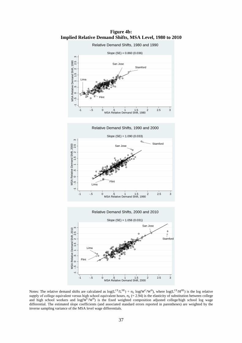
37

Figure 4b: Implied Relative Demand Shifts, MSA Level, 1980 to 2010

StamfordSan Jose

Lima

Flint

-1-.5

0.5

11.

52

2.5

3M

SA R

elat

ive

Dem

and

Shift

, 199

0

-1 -.5 0 .5 1 1.5 2 2.5 3MSA Relative Demand Shift, 1980

Slope (SE) = 0.860 (0.036)


StamfordSan Jose

LimaFlint

-1-.5

0.5

11.

52

2.5

3M

SA

Rel

ativ

e D

eman

d S

hift,

200

0


Slope (SE) = 1.090 (0.033)


Stamford

San Jose

Lima

Flint

-1-.5

0.5

11.

52

2.5

3M

SA

Rel

ativ

e D

eman

d S

hift,

201

0


Slope (SE) = 1.056 (0.031)


Notes: The relative demand shifts are calculated as log(LCE/LHE) + σE log(WC/WH), where log(LCE/HHE) is the log relative supply of college equivalent versus high school equivalent hours, σE (= 2.94) is the elasticity of substitution between college and high school workers and log(WC/WH) is the fixed weighted composition adjusted college/high school log wage differential. The estimated slope coefficients (and associated standard errors reported in parentheses) are weighted by the inverse sampling variance of the MSA level wage differentials.

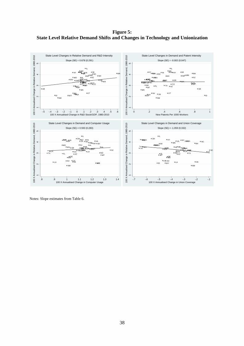
38

Figure 5: State Level Relative Demand Shifts and Changes in Technology and Unionization

DE

IDNM

WY

WV

NY

NV

MO

FL

OK

TN

AZ

LA

MT

PA

MD

KY

MS

OH

VT

MEIA

KSARSD

GAVA

SC

TXNEND

IN

AL

IL

WI

UT

RICA

MNNJ

CT

MI

CO

NCNH

ORWA

MA

12

34

5

-.5 -.4 -.3 -.2 -.1 0 .1 .2 .3 .4 .5 .6

100

X A

nnua

lised

Cha

nge

in R

elat

ive

Dem

and,

198

0-20

10

Slope (SE) = 0.678 (0.291)

100 X Annualised Change in R&D Stock/GDP, 1980-2010

State Level Changes in Relative Demand and R&D Intensity

ID

DE

CA

NJ

MA

VTCT

MNNH

MI

WAOR

NY

CO

IL

AZ

PAOH

UT

WI

TX

MDRI

IN

OK

NC

NM

IA

FL

VA

MO

NV

GA

KSTNSC

KY

LA

MEWV

MT

NE

WY

ND

ALSDAR

MS

12

34

5

0 .2 .4 .6 .8 1

100

X A

nnua

lised

Cha

nge

in R

elat

ive

Dem

and,

198

0-20

10

Slope (SE) = -0.002 (0.047)

New Patents Per 1000 Workers

State Level Changes in Demand and Patent Intensity

TXCA

LA

MO

FL

NYMI

WV

NV

MA

NM

MS

IN

DE

OR

UTOK

COAZ

OH

AR

NJ

GA

CTMD

KY

RISD

IL

NE

ME

NCPA

TN

VT

IAMN

WAKS

NHVA

WY

WI

ID

ND

AL

MT

SC

12

34

5

.8 .9 1 1.1 1.2 1.3 1.4

100

X A

nnua

lised

Cha

nge

in R

elat

ive

Dem

and,

198

0-20

10

Slope (SE) = 0.593 (0.283)

100 X Annualised Change in Computer Usage

State Level Changes in Demand and Computer Usage

SCVT

NC

OK

NH

NM

NETXAR

GAMA

RICA

KSOR

NY

SD

ME

AZCOCT

VA

LA

AL

ND

MN

DE

KY

MS

NVWY

MDWA

UT

FL

WI

MT

IL

ID

MONJIA

OHPAIN

WV

MI

TN

12

34

5

-.7 -.6 -.5 -.4 -.3 -.2 -.1

100

X A

nnua

lised

Cha

nge

in R

elat

ive

Dem

and,

198

0-20

10Slope (SE) = -1.059 (0.332)

100 X Annualised Change in Union Coverage

State Level Changes in Demand and Union Coverage

Notes: Slope estimates from Table 6.

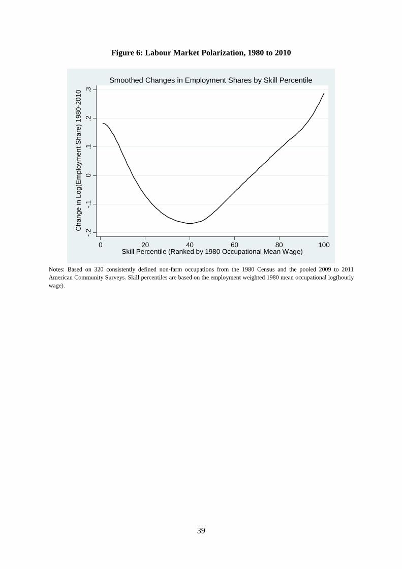
39

Figure 6: Labour Market Polarization, 1980 to 2010

-.2-.1

0.1

.2.3

0 20 40 60 80 100Skill Percentile (Ranked by 1980 Occupational Mean Wage)

Cha

nge

in L

og(E

mpl

oym

ent S

hare

) 198

0-20

10Smoothed Changes in Employment Shares by Skill Percentile

Notes: Based on 320 consistently defined non-farm occupations from the 1980 Census and the pooled 2009 to 2011 American Community Surveys. Skill percentiles are based on the employment weighted 1980 mean occupational log(hourly wage).

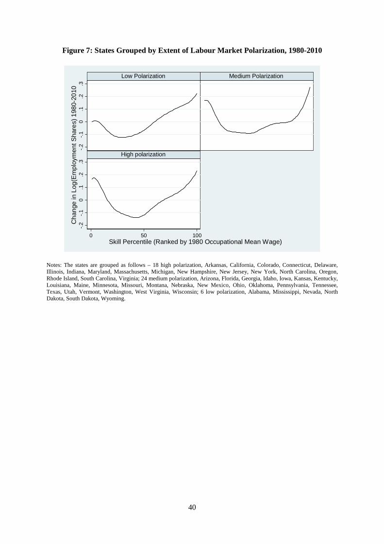
40

Figure 7: States Grouped by Extent of Labour Market Polarization, 1980-2010

-.2-.1

0.1

.2.3

-.2-.1

0.1

.2.3

0 50 100

Low Polarization Medium Polarization

High polarization

Cha

nge

in L

og(E

mpl

oym

ent S

hare

s) 1

980-

2010

Skill Percentile (Ranked by 1980 Occupational Mean Wage)

Notes: The states are grouped as follows – 18 high polarization, Arkansas, California, Colorado, Connecticut, Delaware, Illinois, Indiana, Maryland, Massachusetts, Michigan, New Hampshire, New Jersey, New York, North Carolina, Oregon, Rhode Island, South Carolina, Virginia; 24 medium polarization, Arizona, Florida, Georgia, Idaho, Iowa, Kansas, Kentucky, Louisiana, Maine, Minnesota, Missouri, Montana, Nebraska, New Mexico, Ohio, Oklahoma, Pennsylvania, Tennessee, Texas, Utah, Vermont, Washington, West Virginia, Wisconsin; 6 low polarization, Alabama, Mississippi, Nevada, North Dakota, South Dakota, Wyoming.

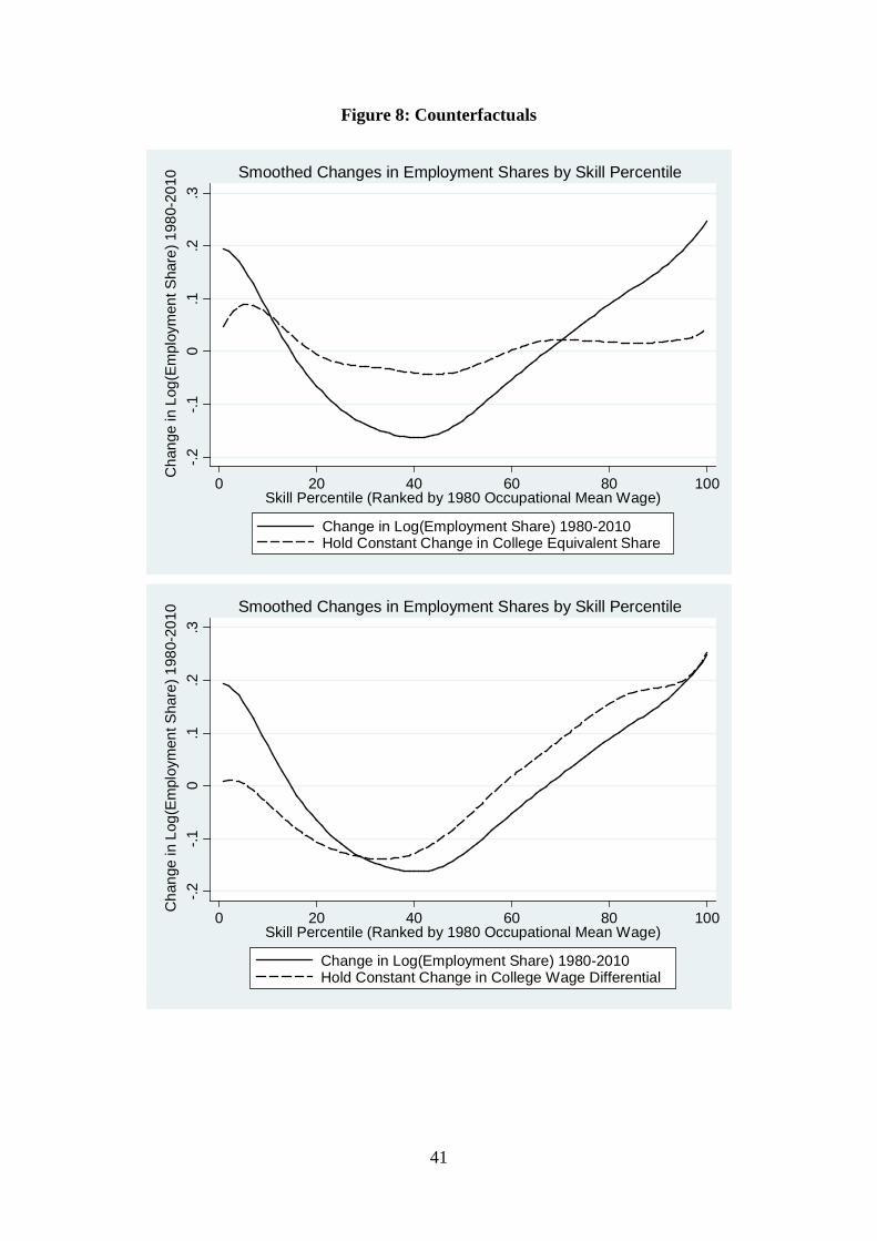
41

Figure 8: Counterfactuals

-.2-.1

0.1

.2.3

0 20 40 60 80 100

Change in Log(Employment Share) 1980-2010Hold Constant Change in College Equivalent Share

Cha

nge

in L

og(E

mpl

oym

ent S

hare

) 198

0-20

10


Smoothed Changes in Employment Shares by Skill Percentile-.2

-.10

.1.2

.3

0 20 40 60 80 100

Change in Log(Employment Share) 1980-2010Hold Constant Change in College Wage Differential

Cha

nge

in L

og(E

mpl

oym

ent S

hare

) 198

0-20

10


Smoothed Changes in Employment Shares by Skill Percentile

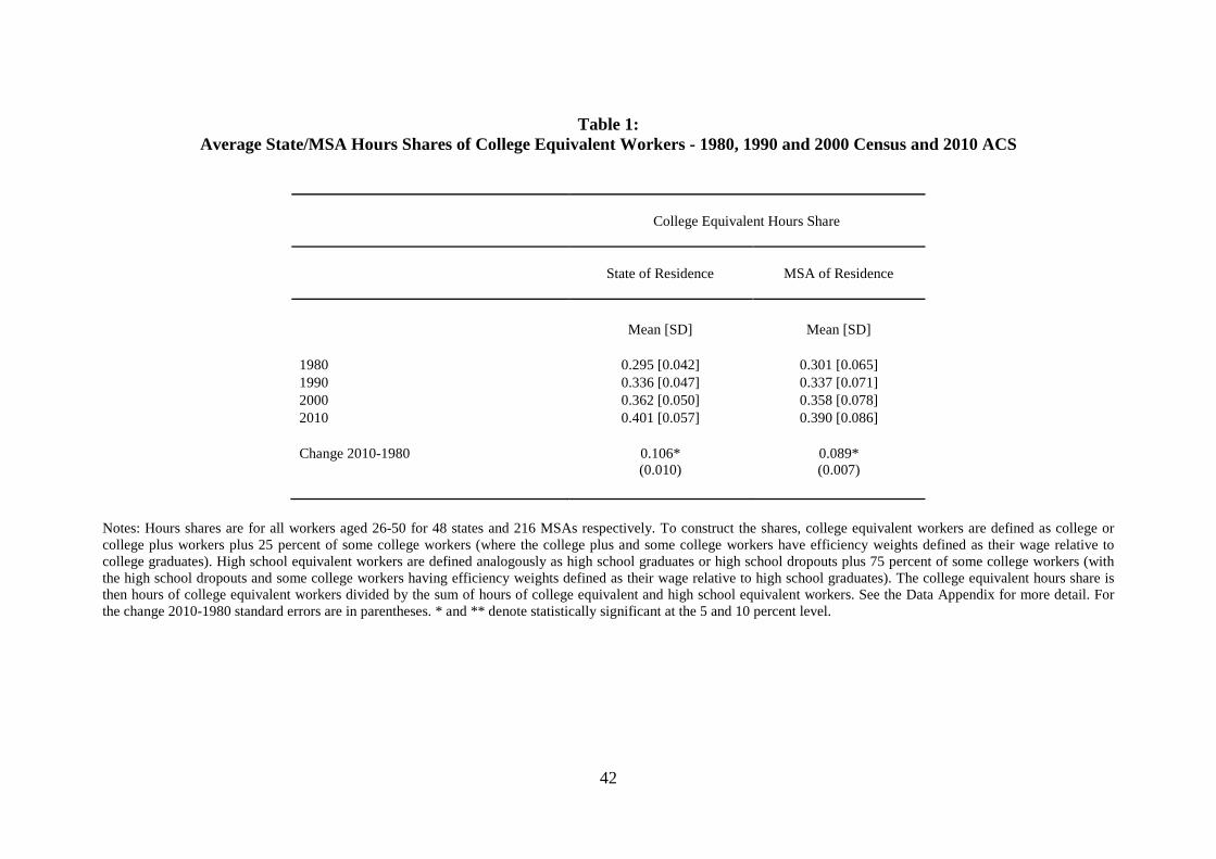
42

Table 1: Average State/MSA Hours Shares of College Equivalent Workers - 1980, 1990 and 2000 Census and 2010 ACS

College Equivalent Hours Share

State of Residence

MSA of Residence

Mean [SD] Mean [SD] 1980 0.295 [0.042] 0.301 [0.065] 1990 0.336 [0.047] 0.337 [0.071] 2000 0.362 [0.050] 0.358 [0.078] 2010 0.401 [0.057] 0.390 [0.086] Change 2010-1980 0.106*

(0.010) 0.089* (0.007)

Notes: Hours shares are for all workers aged 26-50 for 48 states and 216 MSAs respectively. To construct the shares, college equivalent workers are defined as college or college plus workers plus 25 percent of some college workers (where the college plus and some college workers have efficiency weights defined as their wage relative to college graduates). High school equivalent workers are defined analogously as high school graduates or high school dropouts plus 75 percent of some college workers (with the high school dropouts and some college workers having efficiency weights defined as their wage relative to high school graduates). The college equivalent hours share is then hours of college equivalent workers divided by the sum of hours of college equivalent and high school equivalent workers. See the Data Appendix for more detail. For the change 2010-1980 standard errors are in parentheses. * and ** denote statistically significant at the 5 and 10 percent level.

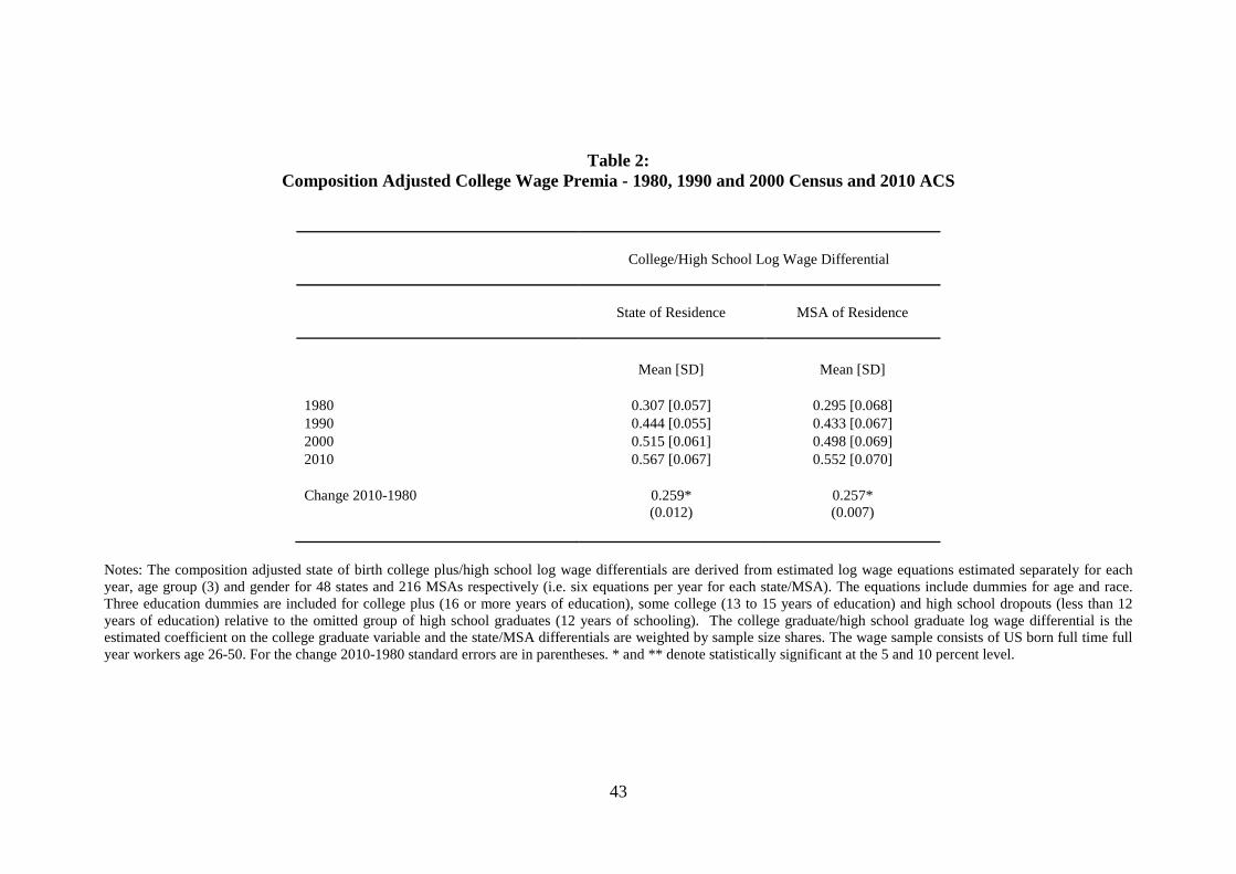
43

Table 2: Composition Adjusted College Wage Premia - 1980, 1990 and 2000 Census and 2010 ACS

College/High School Log Wage Differential

State of Residence

MSA of Residence

Mean [SD] Mean [SD] 1980 0.307 [0.057] 0.295 [0.068] 1990 0.444 [0.055] 0.433 [0.067] 2000 0.515 [0.061] 0.498 [0.069] 2010 0.567 [0.067] 0.552 [0.070] Change 2010-1980 0.259*

(0.012) 0.257* (0.007)

Notes: The composition adjusted state of birth college plus/high school log wage differentials are derived from estimated log wage equations estimated separately for each year, age group (3) and gender for 48 states and 216 MSAs respectively (i.e. six equations per year for each state/MSA). The equations include dummies for age and race. Three education dummies are included for college plus (16 or more years of education), some college (13 to 15 years of education) and high school dropouts (less than 12 years of education) relative to the omitted group of high school graduates (12 years of schooling). The college graduate/high school graduate log wage differential is the estimated coefficient on the college graduate variable and the state/MSA differentials are weighted by sample size shares. The wage sample consists of US born full time full year workers age 26-50. For the change 2010-1980 standard errors are in parentheses. * and ** denote statistically significant at the 5 and 10 percent level.

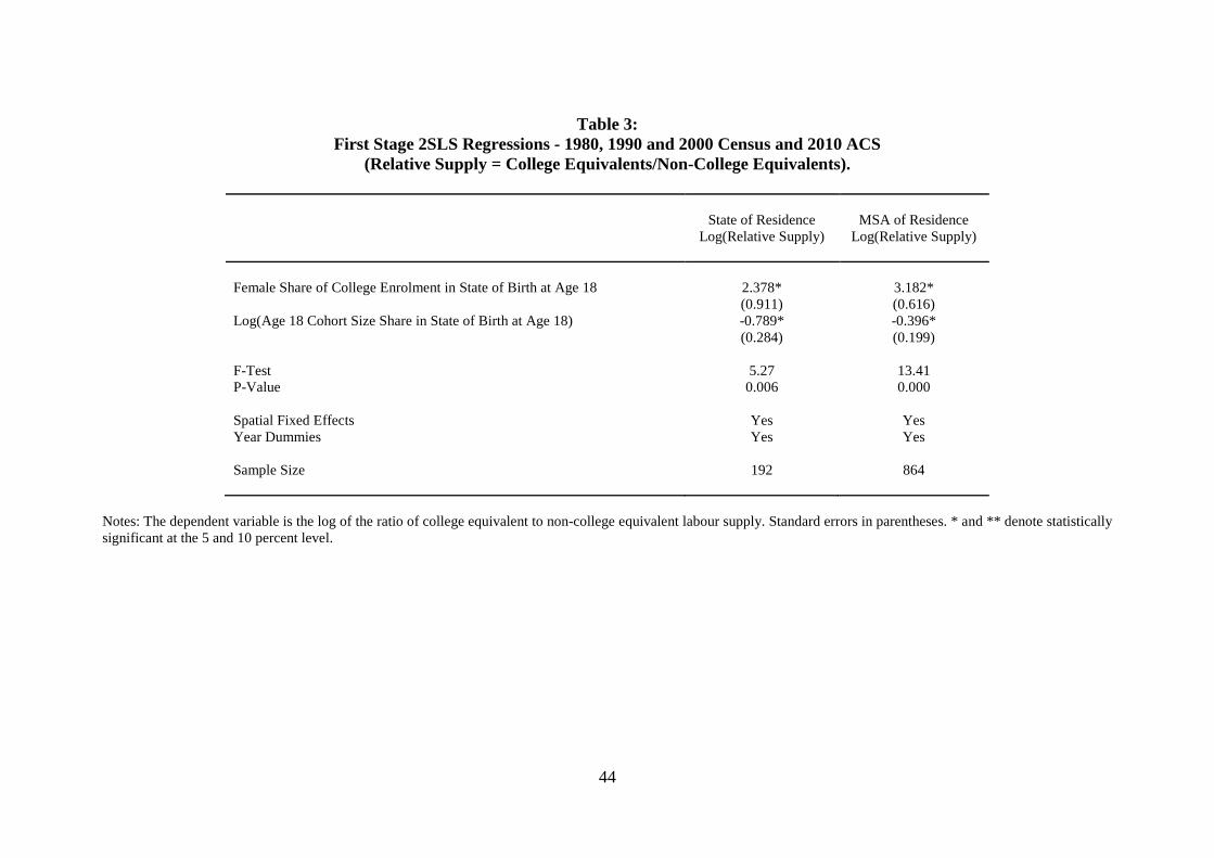
44

Table 3: First Stage 2SLS Regressions - 1980, 1990 and 2000 Census and 2010 ACS

(Relative Supply = College Equivalents/Non-College Equivalents).

State of Residence

Log(Relative Supply)

MSA of Residence

Log(Relative Supply)

Female Share of College Enrolment in State of Birth at Age 18 2.378*

(0.911) 3.182* (0.616)

Log(Age 18 Cohort Size Share in State of Birth at Age 18) -0.789* (0.284)

-0.396* (0.199)

F-Test 5.27 13.41 P-Value 0.006 0.000 Spatial Fixed Effects Yes Yes Year Dummies Yes Yes

Sample Size 192 864

Notes: The dependent variable is the log of the ratio of college equivalent to non-college equivalent labour supply. Standard errors in parentheses. * and ** denote statistically significant at the 5 and 10 percent level.

45

Table 4: 2SLS Estimates of Supply-Demand Models of College Plus/High School Wage Differentials - 1980, 1990 and 2000 Census and 2010 ACS

(Relative Supply = College Equivalents/Non-College Equivalents)

State of Residence

Log(Relative Wage)

MSA of Residence

Log(Relative Wage)

Log(Relative Supply) -0.489*

(0.186) -0.340* (0.098)

Year = 1990 0.247* (0.040)

0.210* (0.022)

Year = 2000 0.391* (0.064)

0.329* (0.032)

Year= 2010 0.532* (0.095)

0.446* (0.048)

Spatial Fixed Effects Yes Yes Sample Size 192 864

Notes: The dependent variable is the log of the composition adjusted college/high school wage differential. The female share of college enrolment in the state of birth at age 18 and the log of the age 18 cohort size in the state of birth at age 18 are used as instruments for Log(Relative Supply) - the first stages are in Table 3. Estimates are weighted by the inverse sampling variance of the state/MSA level wage differentials. Standard errors in parentheses. * and ** denote statistically significant at the 5 and 10 percent level.

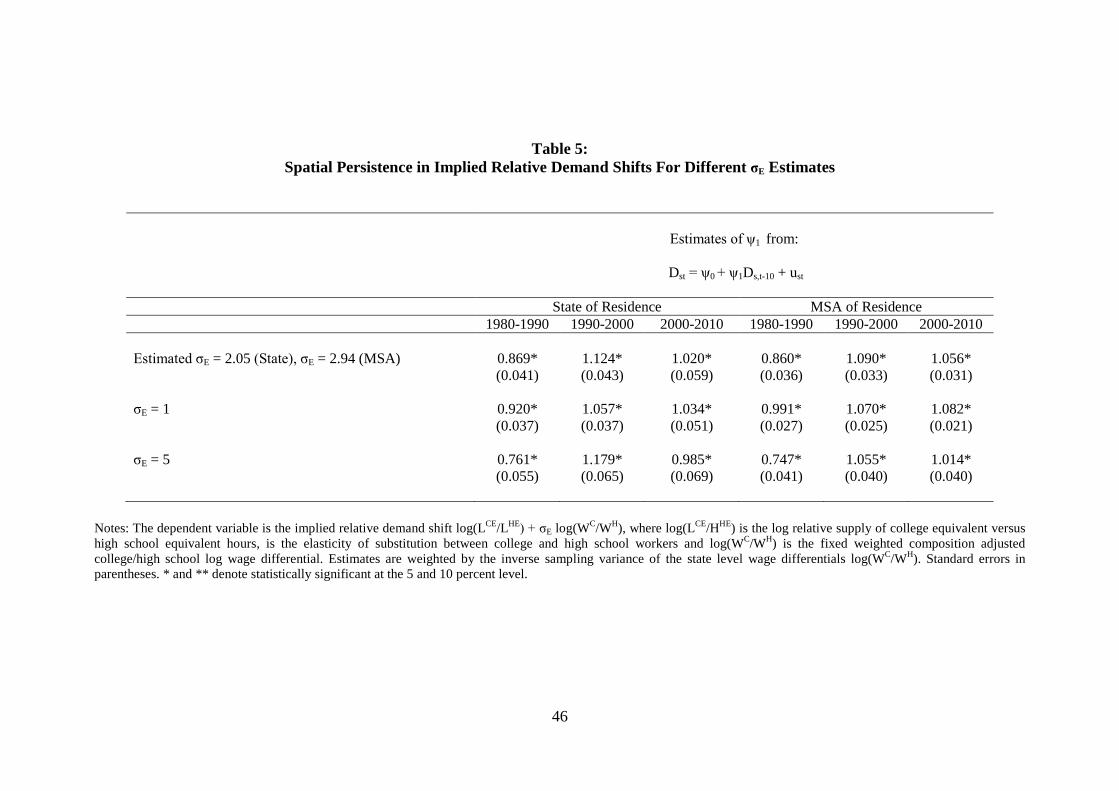
46

Table 5: Spatial Persistence in Implied Relative Demand Shifts For Different σE Estimates

Estimates of ψ1 from:

Dst = ψ0 + ψ1Ds,t-10 + ust

State of Residence MSA of Residence 1980-1990 1990-2000 2000-2010 1980-1990 1990-2000 2000-2010 Estimated σE = 2.05 (State), σE = 2.94 (MSA) 0.869*

(0.041) 1.124* (0.043)

1.020* (0.059)

0.860* (0.036)

1.090* (0.033)

1.056* (0.031)

σE = 1 0.920*

(0.037) 1.057* (0.037)

1.034* (0.051)

0.991* (0.027)

1.070* (0.025)

1.082* (0.021)

σE = 5 0.761*

(0.055) 1.179* (0.065)

0.985* (0.069)

0.747* (0.041)

1.055* (0.040)

1.014* (0.040)

Notes: The dependent variable is the implied relative demand shift log(LCE/LHE) + σE log(WC/WH), where log(LCE/HHE) is the log relative supply of college equivalent versus high school equivalent hours, is the elasticity of substitution between college and high school workers and log(WC/WH) is the fixed weighted composition adjusted college/high school log wage differential. Estimates are weighted by the inverse sampling variance of the state level wage differentials log(WC/WH). Standard errors in parentheses. * and ** denote statistically significant at the 5 and 10 percent level.

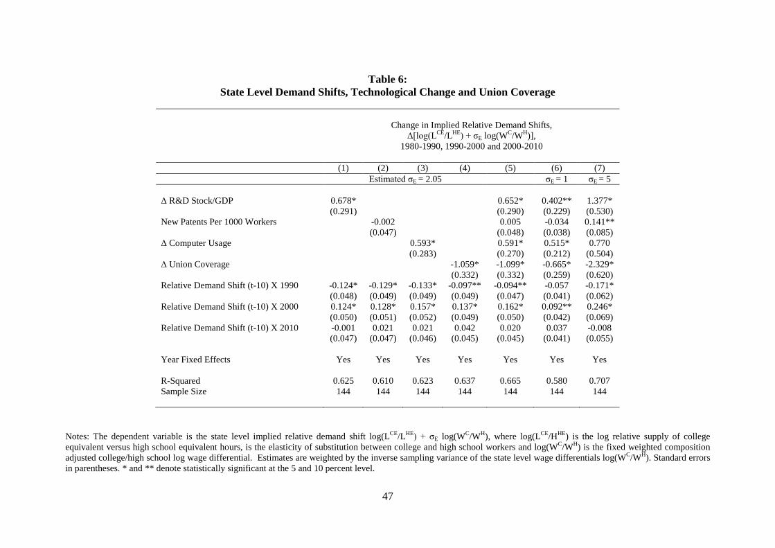
47

Table 6: State Level Demand Shifts, Technological Change and Union Coverage

Change in Implied Relative Demand Shifts, Δ[log(LCE/LHE) + σE log(WC/WH)],

1980-1990, 1990-2000 and 2000-2010

(1) (2) (3) (4) (5) (6) (7) Estimated σE = 2.05 σE = 1 σE = 5 Δ R&D Stock/GDP 0.678*

(0.291) 0.652*

(0.290) 0.402** (0.229)

1.377* (0.530)

New Patents Per 1000 Workers -0.002 (0.047)

0.005 (0.048)

-0.034 (0.038)

0.141** (0.085)

Δ Computer Usage 0.593* (0.283)

0.591* (0.270)

0.515* (0.212)

0.770 (0.504)

Δ Union Coverage -1.059* (0.332)

-1.099* (0.332)

-0.665* (0.259)

-2.329* (0.620)

Relative Demand Shift (t-10) X 1990 -0.124* (0.048)

-0.129* (0.049)

-0.133* (0.049)

-0.097** (0.049)

-0.094** (0.047)

-0.057 (0.041)

-0.171* (0.062)

Relative Demand Shift (t-10) X 2000 0.124* (0.050)

0.128* (0.051)

0.157* (0.052)

0.137* (0.049)

0.162* (0.050)

0.092** (0.042)

0.246* (0.069)

Relative Demand Shift (t-10) X 2010 -0.001 (0.047)

0.021 (0.047)

0.021 (0.046)

0.042 (0.045)

0.020 (0.045)

0.037 (0.041)

-0.008 (0.055)

Year Fixed Effects Yes Yes Yes Yes Yes Yes Yes R-Squared 0.625 0.610 0.623 0.637 0.665 0.580 0.707 Sample Size 144 144 144 144 144 144 144

Notes: The dependent variable is the state level implied relative demand shift log(LCE/LHE) + σE log(WC/WH), where log(LCE/HHE) is the log relative supply of college equivalent versus high school equivalent hours, is the elasticity of substitution between college and high school workers and log(WC/WH) is the fixed weighted composition adjusted college/high school log wage differential. Estimates are weighted by the inverse sampling variance of the state level wage differentials log(WC/WH). Standard errors in parentheses. * and ** denote statistically significant at the 5 and 10 percent level.

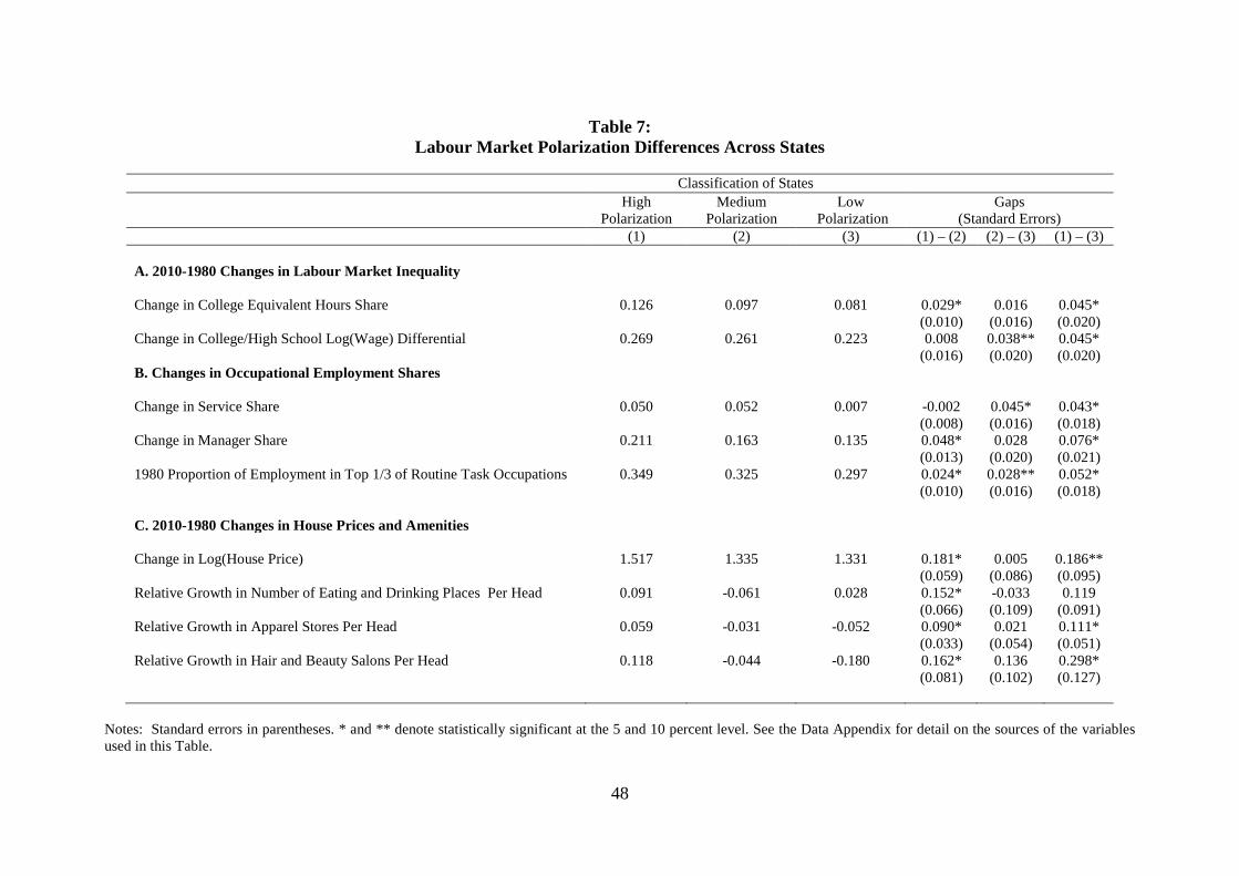
48

Table 7: Labour Market Polarization Differences Across States

Classification of States High

Polarization Medium

Polarization Low

Polarization Gaps

(Standard Errors) (1) (2) (3) (1) – (2) (2) – (3) (1) – (3) A. 2010-1980 Changes in Labour Market Inequality Change in College Equivalent Hours Share 0.126 0.097 0.081 0.029*

(0.010) 0.016

(0.016) 0.045* (0.020)

Change in College/High School Log(Wage) Differential 0.269 0.261 0.223 0.008 (0.016)

0.038** (0.020)

0.045* (0.020)

B. Changes in Occupational Employment Shares Change in Service Share 0.050 0.052 0.007 -0.002

(0.008) 0.045* (0.016)

0.043* (0.018)

Change in Manager Share 0.211 0.163 0.135 0.048* (0.013)

0.028 (0.020)

0.076* (0.021)

1980 Proportion of Employment in Top 1/3 of Routine Task Occupations 0.349 0.325 0.297 0.024* (0.010)

0.028** (0.016)

0.052* (0.018)

C. 2010-1980 Changes in House Prices and Amenities Change in Log(House Price) 1.517 1.335 1.331 0.181*

(0.059) 0.005

(0.086) 0.186** (0.095)

Relative Growth in Number of Eating and Drinking Places Per Head 0.091 -0.061 0.028 0.152* (0.066)

-0.033 (0.109)

0.119 (0.091)

Relative Growth in Apparel Stores Per Head 0.059 -0.031 -0.052 0.090* (0.033)

0.021 (0.054)

0.111* (0.051)

Relative Growth in Hair and Beauty Salons Per Head 0.118 -0.044 -0.180 0.162* (0.081)

0.136 (0.102)

0.298* (0.127)

Notes: Standard errors in parentheses. * and ** denote statistically significant at the 5 and 10 percent level. See the Data Appendix for detail on the sources of the variables used in this Table.

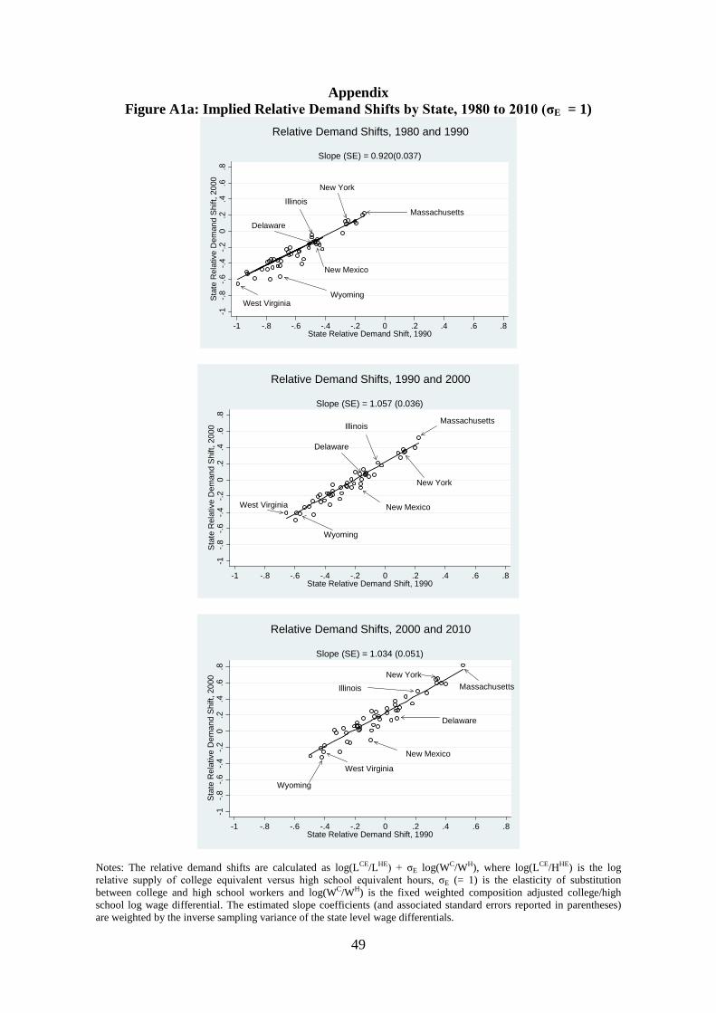
49

Appendix Figure A1a: Implied Relative Demand Shifts by State, 1980 to 2010 (σE = 1)

Massachusetts

New York


Illinois

Delaware

New Mexico

-1-.8

-.6-.4

-.20

.2.4

.6.8

Sta

te R

elat

ive

Dem

and

Shi

ft, 2

000

-1 -.8 -.6 -.4 -.2 0 .2 .4 .6 .8State Relative Demand Shift, 1990

Slope (SE) = 0.920(0.037)


Massachusetts

New York

West Virginia

Wyoming

Illinois

Delaware

New Mexico

-1-.8

-.6-.4

-.20

.2.4

.6.8

Sta

te R

elat

ive

Dem

and

Shi

ft, 2

000


Slope (SE) = 1.057 (0.036)


MassachusettsNew York

Wyoming

West Virginia

New Mexico

Delaware

Illinois

-1-.8

-.6-.4

-.20

.2.4

.6.8

Sta

te R

elat

ive

Dem

and

Shi

ft, 2

000


Slope (SE) = 1.034 (0.051)


Notes: The relative demand shifts are calculated as log(LCE/LHE) + σE log(WC/WH), where log(LCE/HHE) is the log relative supply of college equivalent versus high school equivalent hours, σE (= 1) is the elasticity of substitution between college and high school workers and log(WC/WH) is the fixed weighted composition adjusted college/high school log wage differential. The estimated slope coefficients (and associated standard errors reported in parentheses) are weighted by the inverse sampling variance of the state level wage differentials.

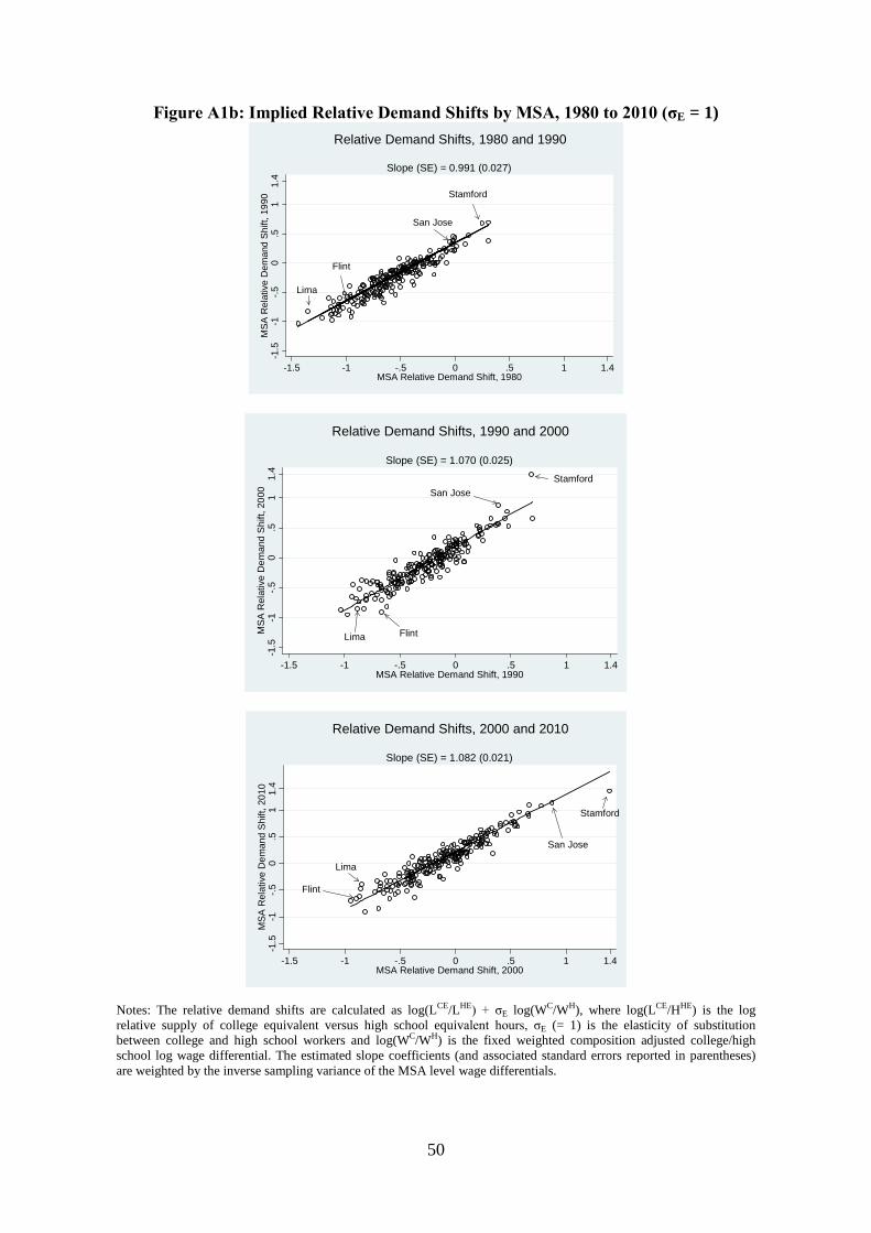
50

Figure A1b: Implied Relative Demand Shifts by MSA, 1980 to 2010 (σE = 1)

Stamford

Lima

Flint

San Jose

-1.5

-1-.5

0.5

11.

4M

SA R

elat

ive

Dem

and

Shift

, 199

0

-1.5 -1 -.5 0 .5 1 1.4MSA Relative Demand Shift, 1980

Slope (SE) = 0.991 (0.027)


StamfordSan Jose

FlintLima

-1.5

-1-.5

0.5

11.

4M

SA

Rel

ativ

e D

eman

d S

hift,

200

0


Slope (SE) = 1.070 (0.025)


Stamford

San Jose

Lima

Flint

-1.5

-1-.5

0.5

11.

4M

SA R

elat

ive

Dem

and

Shift

, 201

0


Slope (SE) = 1.082 (0.021)


Notes: The relative demand shifts are calculated as log(LCE/LHE) + σE log(WC/WH), where log(LCE/HHE) is the log relative supply of college equivalent versus high school equivalent hours, σE (= 1) is the elasticity of substitution between college and high school workers and log(WC/WH) is the fixed weighted composition adjusted college/high school log wage differential. The estimated slope coefficients (and associated standard errors reported in parentheses) are weighted by the inverse sampling variance of the MSA level wage differentials.

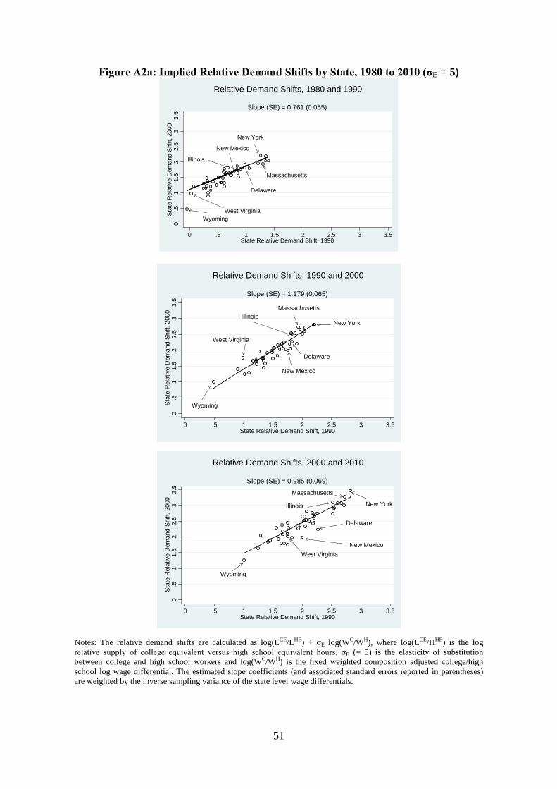
51

Figure A2a: Implied Relative Demand Shifts by State, 1980 to 2010 (σE = 5)

Massachusetts

New York


Delaware

New Mexico

Illinois

0.5

11.

52

2.5

33.

5St

ate

Rel

ativ

e D

eman

d Sh

ift, 2

000

0 .5 1 1.5 2 2.5 3 3.5State Relative Demand Shift, 1990

Slope (SE) = 0.761 (0.055)


New York

Massachusetts

West Virginia

Wyoming

Delaware

New Mexico

Illinois

0.5

11.

52

2.5

33.

5S

tate

Rel

ativ

e D

eman

d S

hift,

200

0


Slope (SE) = 1.179 (0.065)


New York

Massachusetts

Wyoming

West Virginia

Illinois

New Mexico

Delaware

0.5

11.

52

2.5

33.

5St

ate

Rel

ativ

e D

eman

d Sh

ift, 2

000


Slope (SE) = 0.985 (0.069)


Notes: The relative demand shifts are calculated as log(LCE/LHE) + σE log(WC/WH), where log(LCE/HHE) is the log relative supply of college equivalent versus high school equivalent hours, σE (= 5) is the elasticity of substitution between college and high school workers and log(WC/WH) is the fixed weighted composition adjusted college/high school log wage differential. The estimated slope coefficients (and associated standard errors reported in parentheses) are weighted by the inverse sampling variance of the state level wage differentials.

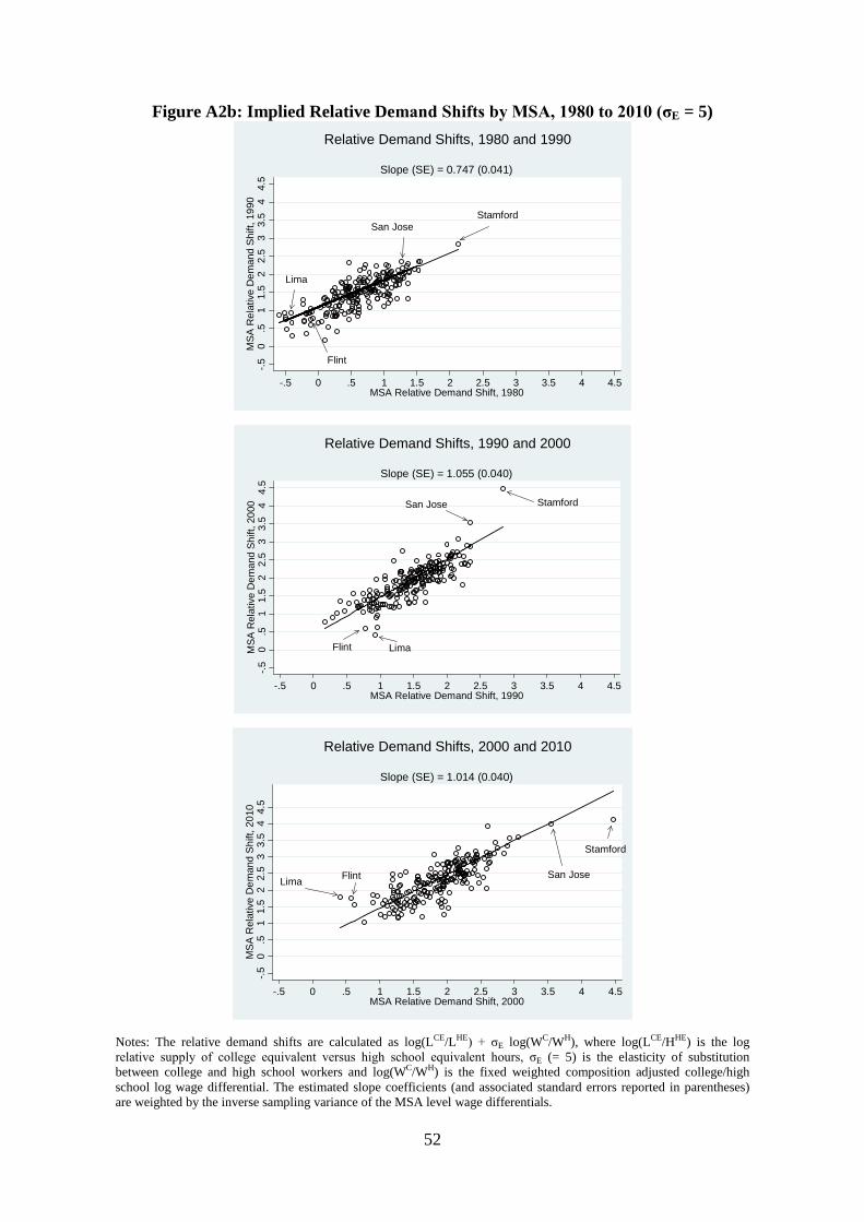
52

Figure A2b: Implied Relative Demand Shifts by MSA, 1980 to 2010 (σE = 5)

StamfordSan Jose

Flint

Lima

-.50

.51

1.5

22.

53

3.5

44.

5M

SA

Rel

ativ

e D

eman

d S

hift,

199

0

-.5 0 .5 1 1.5 2 2.5 3 3.5 4 4.5MSA Relative Demand Shift, 1980

Slope (SE) = 0.747 (0.041)


StamfordSan Jose

LimaFlint

-.50

.51

1.5

22.

53

3.5

44.

5M

SA

Rel

ativ

e D

eman

d S

hift,

200

0


Slope (SE) = 1.055 (0.040)


Stamford

San JoseFlintLima

-.50

.51

1.5

22.

53

3.5

44.

5M

SA

Rel

ativ

e D

eman

d S

hift,

201

0


Slope (SE) = 1.014 (0.040)


Notes: The relative demand shifts are calculated as log(LCE/LHE) + σE log(WC/WH), where log(LCE/HHE) is the log relative supply of college equivalent versus high school equivalent hours, σE (= 5) is the elasticity of substitution between college and high school workers and log(WC/WH) is the fixed weighted composition adjusted college/high school log wage differential. The estimated slope coefficients (and associated standard errors reported in parentheses) are weighted by the inverse sampling variance of the MSA level wage differentials.

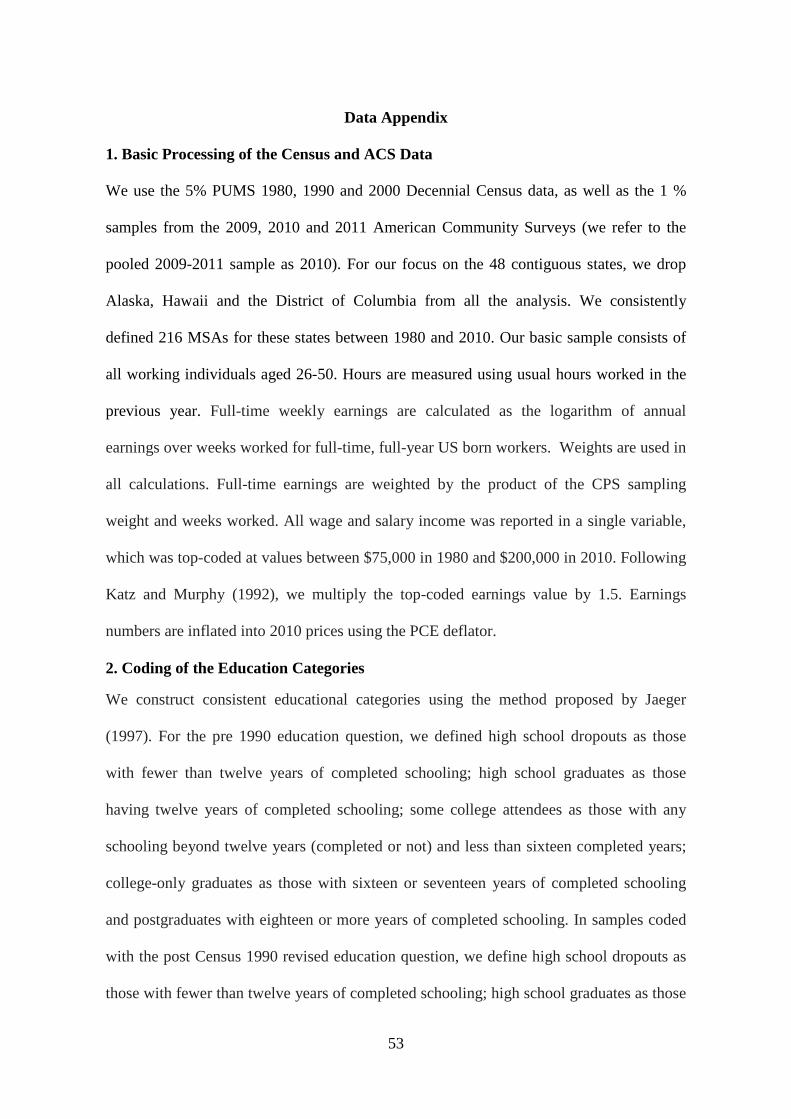
53

Data Appendix

1. Basic Processing of the Census and ACS Data

We use the 5% PUMS 1980, 1990 and 2000 Decennial Census data, as well as the 1 %

samples from the 2009, 2010 and 2011 American Community Surveys (we refer to the

pooled 2009-2011 sample as 2010). For our focus on the 48 contiguous states, we drop

Alaska, Hawaii and the District of Columbia from all the analysis. We consistently

defined 216 MSAs for these states between 1980 and 2010. Our basic sample consists of

all working individuals aged 26-50. Hours are measured using usual hours worked in the

previous year. Full-time weekly earnings are calculated as the logarithm of annual

earnings over weeks worked for full-time, full-year US born workers. Weights are used in

all calculations. Full-time earnings are weighted by the product of the CPS sampling

weight and weeks worked. All wage and salary income was reported in a single variable,

which was top-coded at values between $75,000 in 1980 and $200,000 in 2010. Following

Katz and Murphy (1992), we multiply the top-coded earnings value by 1.5. Earnings

numbers are inflated into 2010 prices using the PCE deflator.

2. Coding of the Education Categories

We construct consistent educational categories using the method proposed by Jaeger

(1997). For the pre 1990 education question, we defined high school dropouts as those

with fewer than twelve years of completed schooling; high school graduates as those

having twelve years of completed schooling; some college attendees as those with any

schooling beyond twelve years (completed or not) and less than sixteen completed years;

college-only graduates as those with sixteen or seventeen years of completed schooling

and postgraduates with eighteen or more years of completed schooling. In samples coded

with the post Census 1990 revised education question, we define high school dropouts as

those with fewer than twelve years of completed schooling; high school graduates as those

54

with either twelve completed years of schooling and/or a high school diploma or G.E.D.;

some college as those attending some college or holding an associate’s degree; college

only as those with a bachelor degree; and postgraduate as a masters, professional or

doctorate degree.

3. Construction of the Relative Wage Series

We calculate composition-adjusted relative wages overall and by age cohorts using the

wage sample described above, excluding the self-employed. The data are sorted into

gender-education-age groups based on a breakdown of the data by gender, the five

education categories described above, and five age/birth cohort categories (ages 26-30, 31-

35, 36-40, 41-45 and 46–50).33 We generate a composition adjusted college plus/high

school graduate wage differential separately by sex and age groups by estimating ten

separate regressions for each state/MSA and year including education and age dummies

(as well as two dummies for race). These are then employment share weighted to form the

(composition-adjusted) college plus/high school graduate wage differential in a given

state/MSA and year. As this is a regression generated variable, when the differential is

used as a dependent variable in regressions in the paper, it is weighted by the inverse

(employment share weighted) sampling variances of the estimated wage differentials.

4. Construction of the Relative Supply Measures

We calculate relative supply measures using the sample above. We form a labour quantity

sample equal to total hours worked by all employed workers (including those in self-

employment) age 26 to 50 to form education cells in each state/MSA and year. Education

groups are high school dropout, high school graduate, some college, college graduate, and

postgraduate. This provides our efficiency units by education group.

33 Within sample years, these are the same as five birth cohorts (e.g. for the 1980 Census, birth cohorts from 1930-34, 1935-39, 1940-44, 1945-49 and 1950-54).

55

The quantity data are merged to a corresponding price sample containing mean

full-time weekly real wages by state/MSA, year and education group (wage data used for

the price sample correspond to the earnings samples described above). For each

state/MSA and year we calculate aggregate college equivalent labour supply as the total

efficiency units of labour supplied by postgraduates weighted by the postgraduate-college

graduate relative wage from the price sample, plus college graduate efficiency units, plus

25 percent of the efficiency units of labour supplied by workers with some college

weighted by the some college-college graduate relative wage. Similarly, aggregate high

school equivalent labour supply is the sum of efficiency units supplied by high school or

lower workers, plus 75 percent of the efficiency units supplied by workers with some

college, all weighted by respective relative high school graduate average wages. Hence,

the college-only/high school log relative supply index is the natural logarithm of the ratio

of college-only equivalent to non-college equivalent labour supply (in efficiency units) in

each state/MSA and year.

5. Instruments in Relative Demand and Supply Models To match to the samples of 26-50 year olds in 1980, 1990, 2000 and 2010, we collected

annual data at state level from 1948 to 2002 on the proportion of women enrolled in

higher education institutions from various yearbook editions (beginning with the 1949

edition) of the Statistical Abstract of the United States (original sources initially being the

Biennial Survey of Education and from 1962 onwards the Digest of Education Statistics).

The size of the age eighteen population was also obtained from for each year from Census

Bureau data by state from 1948 to 2002. The female share of college enrolment and the

age 18 cohort size as a proportion of the total state population were then matched to the

individual Census and ACS data by state of birth and year aged 18.

56

6. Technology and Union Data Our Research and Development (R&D) intensity measures are generated using R&D

expenditure divided by nominal GDP for 1977, 1987, 1997 and 2007. These are taken

from the National Industrial Productivity Accounts (NIPA) made available by the Bureau

of Economic Analysis. State level changes in R&D performance are measured using Total

(company, Federal and Other) funds for industrial R&D performance in millions of

dollars.

The patents data come from the US Patent and Trademark Office (USPO). We use

total annual utility patents granted by state and year, December 2011.34 We define new

patents as the state level of patents in 1980, 1990, 2000 and 2010. We use Census state

level employment numbers to express these as new patents per worker.

The computer use data are measured in proportions per state in each year. These

are taken from the October 1984, 1987, 1997 and 2003 CPS supplements and derived

from the question `Do you use a computer at work?’. Computer use is the proportion of

employed workers in the CPS that use computers at work.

The union coverage data are also in state level proportions per year and are taken

from the Union Membership and Coverage Database provided by Hirsch and Macpherson

(2003).35 These are generated using CPS data beginning in 1973 and are updated annually.

7. Labour Market Polarization

The skill percentiles are based upon 320 consistently defined occupations for all those in

employment from the 1980 Census and 2010 American Community Survey. The

procedures followed in Autor and Dorn (2013) and Lefter and Sand (2011) are used to

obtain the consistent definitions. The 320 occupations are divided into employment

weighted percentiles based upon the mean occupational wage in 1980.

34 These are available to download at http://www.uspto.gov/web/offices/ac/ido/oeip/taf/cst_utlh.htm/. 35 These data are available to download from http://www.unionstats.com/.

http://www.uspto.gov/web/offices/ac/ido/oeip/taf/cst_utlh.htm/

http://www.unionstats.com/

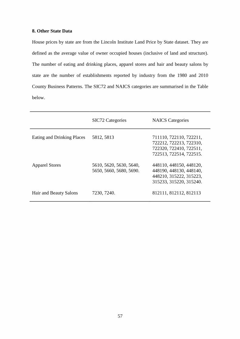
57

8. Other State Data

House prices by state are from the Lincoln Institute Land Price by State dataset. They are

defined as the average value of owner occupied houses (inclusive of land and structure).

The number of eating and drinking places, apparel stores and hair and beauty salons by

state are the number of establishments reported by industry from the 1980 and 2010

County Business Patterns. The SIC72 and NAICS categories are summarised in the Table

below.

SIC72 Categories

NAICS Categories

Eating and Drinking Places

5812, 5813

711110, 722110, 722211, 722212, 722213, 722310, 722320, 722410, 722511, 722513, 722514, 722515.

Apparel Stores 5610, 5620, 5630, 5640, 5650, 5660, 5680, 5690.

448110, 448150, 448120, 448190, 448130, 448140, 448210, 315222, 315223, 315233, 315220, 315240.

Hair and Beauty Salons 7230, 7240. 812111, 812112, 812113

Documents

Spatial Changes in Labour Market Inequality - Iza