Spectral reflectance of coral reef bottom-types worldwide and ...optics.marine.usf.edu/~hu/scratch/jpl_ref/Hochberg_RSE.pdf · Spectral reflectance of coral reef bottom-types worldwide

Spectral reflectance of coral reef bottom-types worldwide and implications

for coral reef remote sensing

Eric J. Hochberga,*, Marlin J. Atkinsona, Serge Andrefouetb

aUniversity of Hawaii, School of Ocean and Earth Science and Technology, Hawaii Institute of Marine Biology, P.O. Box 1346, Kaneohe, HI 96744, USAbUniversity of South Florida, College of Marine Science, Institute for Marine Remote Sensing, St. Petersburg, FL, USA

Received 10 June 2002; received in revised form 11 October 2002; accepted 15 October 2002

Abstract

Coral reef benthic communities are mosaics of individual bottom-types that are distinguished by their taxonomic composition and

functional roles in the ecosystem. Knowledge of community structure is essential to understanding many reef processes. To develop

techniques for identification and mapping of reef bottom-types using remote sensing, we measured 13,100 in situ optical reflectance spectra

(400–700 nm, 1-nm intervals) of 12 basic reef bottom-types in the Atlantic, Pacific, and Indian Oceans: fleshy (1) brown, (2) green, and (3)

red algae; non-fleshy (4) encrusting calcareous and (5) turf algae; (6) bleached, (7) blue, and (8) brown hermatypic coral; (9) soft/gorgonian

coral; (10) seagrass; (11) terrigenous mud; and (12) carbonate sand. Each bottom-type exhibits characteristic spectral reflectance features that

are conservative across biogeographic regions. Most notable are the brightness of carbonate sand and local extrema near 570 nm in blue

(minimum) and brown (maximum) corals. Classification function analyses for the 12 bottom-types achieve mean accuracies of 83%, 76%,

and 71% for full-spectrum data (301-wavelength), 52-wavelength, and 14-wavelength subsets, respectively. The distinguishing spectral

features for the 12 bottom-types exist in well-defined, narrow (10–20 nm) wavelength ranges and are ubiquitous throughout the world. We

reason that spectral reflectance features arise primarily as a result of spectral absorption processes. Radiative transfer modeling shows that in

typically clear coral reef waters, dark substrates such as corals have a depth-of-detection limit on the order of 10–20 m. Our results provide

the foundation for design of a sensor with the purpose of assessing the global status of coral reefs.

Published by Elsevier Science Inc.

Keywords: Coral reef; Spectral reflectance; Remote sensing; Radiative transfer

1. Introduction

Coral reef benthic ecosystems are collections of distinctive

communities, which are distinguished by their characteristic

assemblages of organisms and substrates (Stoddart, 1969). A

benthic community’s structure is defined by its component

set of organisms and substrates; hereafter, we refer to these

fundamental elements of the community as ‘‘bottom-types.’’

Several reef communities may share bottom-types in com-

mon, but the bottom-types’ proportional contributions vary

both between and within communities. From this viewpoint,

all reef communities are simply combinations of some

comprehensive set of bottom-types.

Quantification of benthic community structure is central

to understanding coral reef ecosystem function. Community

structure determines rates of reef metabolism (Kinsey, 1985)

and indicates reef status (Connell, 1997). Different bottom-

types are important in life history strategies of reef-dwelling

organisms, e.g., as recruitment sites for coral larvae (Miller

et al., 2000) and juvenile fish (Light & Jones, 1997), and as

habitat for adult fish (Chabanet et al., 1997). Reef com-

munity structure exhibits tremendous spatial heterogeneity

over scales of centimeters to hundreds of meters and, in

contrast to phytoplankton and macrophyte communities, is

inherently stable on time scales of months to years (Budde-

meier & Smith, 1999). Reports of reef degradation world-

wide (Wilkinson, 2000) are now fueling interest in—and

debate over the causes of—temporal shifts in community

structure on longer time scales.

Conventional methods for determining benthic commun-

ity structure include the use of in situ quadrats, line transects,

and manta tows (Miller & Muller, 1999). These are not

feasible means for accurate determination of bottom-type

spatial distributions over large areas (Ginsburg, 1994).

Digital remote sensing is the most cost-effective approach

for acquiring such data (Mumby, Green, Edwards, & Clark,

0034-4257/03/$ - see front matter. Published by Elsevier Science Inc.

doi:10.1016/S0034-4257(02)00201-8

* Corresponding author. Tel.: +1-808-956-9108; fax: +1-808-956-7112.

E-mail address: [email protected] (E.J. Hochberg).

www.elsevier.com/locate/rse

Remote Sensing of Environment 85 (2003) 159–173

1999), and it is the only available tool to acquire such data on

a global scale. Accepting the need to quantify reef commun-

ity structure through time and over large areas, and accepting

the fact that remote sensing is the most promising tool for the

task, the next obvious step is to develop techniques for using

remote sensing data to detect, discriminate, and quantify the

spatial distributions of reef bottom-types.

Since its inception in the early 1970s, digital remote

sensing of coral reefs has generally followed a sensor-down

approach, in which scene-specific image statistics drive

image classification and interpretation. This approach is

intensely interactive and is largely a product of the fact that

the limited capabilities of available sensors have tended to

generate ambiguous image classification results, requiring

significant human interpretation. In truth, the sensor-down

approach has proven very useful at characterizing reef

geomorphology (reviewed extensively in Green et al.,

1996). With expert knowledge of local reef systems, the

same approach has also been successful for delineation of

whole communities, which are defined a priori to image

classification and, unfortunately, are semi-quantitative at

best (e.g., Andrefouet & Payri, 2001; Mumby, Green, Clark,

& Edwards, 1998). The few attempts to directly detect

fundamental bottom-types—and thus quantify community

structure—have utilized a reef-up approach, in which the

classifier statistics are defined independently of an image

data set (e.g., Hochberg & Atkinson, 2000). In this deter-

ministic approach, the reflectance spectra of bottom-types

are catalogued, and their characteristic features are targeted

through remote sensing. Since all community structures are

defined as subsets of a comprehensive set of bottom-types,

the classifier statistics are applicable across the geographic

area encompassed by the catalog of spectral reflectance data.

Whatever the approach, to be useful in mapping reef

community structure, a remote sensing system must have

the abilities to spatially resolve reef bottom-types and to spec-

trally discriminate between them. Several imaging systems

are currently operational and have specific strategies for coral

reef image acquisition. However, those systems that provide

more spectral information have poor spatial resolution. For

example, SeaWiFS has six narrow wavebands in the visible

spectrum, and MODIS has seven, but these sensors achieve

only 1-km and 250-m pixel resolution, respectively, preclud-

ing their use for spatially discriminating reef bottom-types or

even most reef communities (Andrefouet et al., 2003). Con-

versely, systems with the ability to spatially resolve reef

bottom-types (e.g., Landsat, Ikonos and Quickbird at 30-,

4-, and 2-m pixel resolutions, respectively) have wavebands

that are not optimized for reef bottom-type spectral discrim-

ination (Andrefouet, Muller-Karger, Hochberg, Hu, &

Carder, 2001; Hochberg & Atkinson, 2003).

It is generally agreed that reef bottom-types are spatially

resolvable by (or at least that they cover significant propor-

tions of) the spatial sampling units of current high-resolution

remote sensors (Mumby & Edwards, 2002). Given the 30-

year history of digital coral reef remote sensing, however,

there is surprisingly scant information on spectral reflectance

(R) for reef bottom-types globally. The following is a brief

review of the literature concerning R for coral reef benthos.

Maritorena, Morel, and Gentili (1994) made in vitro

reflectance measurements of carbonate sand, Sargassum

sp., Turbinaria sp., Boodlea sp., Porolithon onkodes, and

Corallinacea sp., but did not examine spectral differences

between the bottom-types. Miyazaki and Harashima (1993)

and Miyazaki, Nakatani, and Harashima (1995) made both

laboratory and in situ measurements of R for nine corals,

rocks, and sand. They visually inspected the spectra and

concluded there were minimal differences between those

three benthic community types. Mazel (1996) examined the

contribution of fluorescence to R, for which he had f 300 in

vivo measurements for 25 coral specimens (10 species).

Holden and LeDrew (1998) made a statistical investigation

on a total of 22 in situ reflectance measurements, representing

bleached and non-bleached Acropora, dead coral rubble, and

algae-covered dead corals. They applied cluster, principal

components and derivative analyses to show that statistically

significant spectral differences could be detected between

healthy Acropora and bleached/dead Acropora. Holden and

LeDrew (1999) measured 133 in situ R’s in Fiji and Sulawesi,

Indonesia for bleached coral, healthy massive corals, healthy

branching corals, dead coral debris, and algae-covered sur-

faces. They performed 181 individual univariate t-tests (one

for each wavelength measured) for each of the classes and

determined that there is no significant spectral difference

between geographic locations within each class. Similar

statistics indicated there is also no spectral difference attrib-

utable to coral morphology, but that there is a difference due

to coral health. Myers, Hardy, Mazel, and Dustan (1999)

reported on five in situ R’s for bleached and pigmented coral

(Montastrea cavernosa), a red crustose alga, a brown algae,

and a red alga (Rhipocephalus phoenix) at Lee Stocking

Island, Bahamas. Their objective was not to discriminate

between the bottom-types but to demonstrate an empirical

relationship between pigmentation and R. In Kaneohe Bay,

Oahu, Hawaii, Hochberg and Atkinson (2000) measured a

total of 247 in situ R’s of three coral species (Montipora

capitata, Porites compressa, Porites lobata), five algal spe-

cies (Dictyosphaeria cavernosa, Gracilaria salicornia, Hal-

imeda sp., Porolithon sp., Sargassum echinocarpum), and

three sand communities (fine-grained carbonate sand, sand

mixed with coral rubble, coral rubble). They used derivative

analysis and the multivariate techniques of stepwise wave-

length selection and linear discriminant analysis to show that

spectral separation of basic bottom-types (coral, algae, and

sand) is possible with as few as four non-contiguous narrow

wavebands. In the lagoon of Rangiroa, French Polynesia,

Clark, Mumby, Chisholm, Jaubert, and Andrefouet (2000)

measured f 1800 in situ R’s for 94 reef targets, including

coral (Porites, Pocillopora, and others), encrusting and turf

algae, and sand. Using derivative analysis, they determined

that it is possible to distinguish between three states of coral

mortality: live coral, coral dead for 6 months, and coral dead

E.J. Hochberg et al. / Remote Sensing of Environment 85 (2003) 159–173160

for >6 months. Joyce and Phinn (2002) analyzed R from

corals with three distinct morphologies (open branching,

closed branching, and table) and determined that the three

are distinguishable by the differing amount of shadow each

morphology generates. Finally, Minghelli-Roman, Chis-

holm, Marchioretti, and Jaubert (2002) measured R for 152

coral colonies in the Red Sea and were able to discriminate

between 14 genera of hard and soft corals using ratios of only

six wavebands. Hedley and Mumby (2002) provide a review

of coral reef R and its biological basis.

These studies represent the greater part of the current state

of knowledge of R for coral reef bottom-types. In their

review, Hedley and Mumby (2002) conclude that ‘‘there is

a great deal of uncertainty and inconsistency in the reported

spectral features that can be employed to discriminate reef

benthos.’’ This is attributable to the fact that the total number

of measurements has been few, methods have been dissimilar

(producing data of varying quality), and objectives have

focused on very localized measurements for a few species.

That is, the database of R for coral reefs is small, and the data

within are nonuniform. As a result, deterministic, reef-up

remote sensing of bottom-types remains impractical, which

in turn precludes quantitative remote sensing of reef com-

munity structure. If remote sensing technology is to be

applied to reef-up assessment of reef community structure,

the first step must be to evaluate the degree to which

fundamental bottom-types can be spectrally discriminated.

Our goals are (1) to characterize spectral reflectance for

reef bottom-types worldwide and (2) to determine spectral

separabilities of the bottom-types. We have used a portable

spectrometer to measure 13,100 in situ R’s at 11 sites in four

major reef biogeographic regions worldwide at water depths

ranging from 0 to 15 m. We assign each measured R to one

of a set of fundamental reef bottom-types, which are defined

primarily by function in the reef system, but also by

taxonomy and by apparent color. We find that each bot-

tom-type exhibits characteristic and distinctive features in R

that exist in well-defined, narrow wavelength ranges and

that are conservative across biogeographic regions. Classi-

fication analysis demonstrates that the bottom-types are

statistically separable and identifiable based on their reflec-

tance spectra. We reason that features in R arise primarily as

a result of spectral absorption processes. Radiative transfer

modeling shows that in typically clear coral reef waters,

dark substrates such as corals have a depth-of-detection

limit on the order of 10–20 m. Our results provide the basis

for quantitative remote sensing of community structure

using consistent criteria for coral reefs worldwide.

2. Methods

2.1. Classification of fundamental bottom-types

Coral reef communities are largely mosaics of coral, va-

rious algae and carbonate sand (Kinsey, 1985), and knowl-

edge of their distributions is fundamental to assessment of

reef status (Connell, 1997; Done, 1992, 1995). Thus, these

three bottom-types form the foundation for our classifica-

tion scheme. There are three basic forms of reef algae: turf

algae, crustose calcareous algae, and fleshy macroalgae

(Berner, 1990). Crustose calcareous algae are important reef

calcifiers (Kinsey, 1985), cementing the products of dis-

integration of various other calcifying reef organisms, thus

creating a harder skin for the reef (Berner, 1990). Turf algae

and fleshy macroalgae are a major source of fixed carbon to

reef primary consumers (Klumpp & McKinnon, 1989).

Because of their importances to different reef processes,

these three algal types form subclasses within the broader

algae class.

While crustose calcareous algae are mainly Rhodophytes

(Corallinaceae), algal turfs are often a mixture of Chlor-

ophytes, Cyanophytes, Phaeophytes, and Rhodophytes

(Berner, 1990) that can mix on spatial scales of < 1 cm,

well beyond the spatial abilities of today’s remote sensors

(smallest footprint f 2 m). However, discounting their

epiphytic communities, fleshy macroalgae—mainly Chlor-

ophytes, Phaeophytes, and Rhodophytes—exist at a spatial

scale (one-tenths to tens of meters) that may be resolvable

by remote sensing. The different fleshy macroalgae taxa are

preferred forage material for different reef consumers

(Glynn, 1990). Furthermore, Chlorophytes, Phaeophytes,

and Rhodophytes possess different photosynthetic accessory

pigments (Kirk, 1994) and thus often exhibit their character-

istic colors of green, brown, and red, respectively. Because

they may be important to understanding energy flow

through the reef system, and because there is potential that

they can be discriminated based on their optical reflectance

spectra, we further separate the fleshy macroalgae subclass

into brown, green, and red divisions.

Soft corals and gorgonians can occupy substantial reef

areas and may compete with scleractinian corals for space

(Bastidas, Benzie, Uthicke, & Fabricius, 2001; Ben-Yosef &

Benayahu, 1999; Fabricius, 1997). Seagrass is essential

habitat in the life histories of many reef species and can

cover extensive back-reef and lagoonal areas (Enrıquez,

Merino, & Iglesias-Prieto, 2002). The spread and deposition

of terrigenous sediments can be deleterious to reefs near

high islands (Watanabe, Nakamura, Samarakoon, Mabuchi,

& Ishibashi, 1993). Because of their respective importances

to coral reef systems, each of these reef bottom-types is

included in the classification scheme.

Examination of the data set has revealed two basic modes

of coral R: one mode is associated with corals that are

visually (to humans) brown, red, orange, yellow, or green,

while the other mode is associated with corals that appear

purple, blue, pink, or gray. These patterns of association

occur across taxonomic lines and in all oceans. Thus, we

divide scleractinian corals into two subclasses, which, for

lack of better terminology, we label ‘‘brown’’ and ‘‘blue.’’

Lastly, the bleached coral subclass is included due to the

prevalence in recent years of reports of coral bleaching

E.J. Hochberg et al. / Remote Sensing of Environment 85 (2003) 159–173 161

worldwide (Wilkinson, 2000). Fig. 1 summarizes the overall

classification scheme adopted for this study.

2.2. Spectral measurements and processing

We measured 13,100 R’s at the following sites in the

Atlantic, Indian, and Pacific Oceans (Fig. 2): (1) St. Croix,

USVI; (2) Puerto Rico; (3) Florida Keys; (4) Oahu, Hawaii;

(5) Maui, Hawaii; (6) Rangiroa, French Polynesia; (7)

Moorea, French Polynesia; (8) Palau; (9) Bali, Indonesia;

(10) Mayotte, Comoros; (11) the Waikiki Aquarium (Indo-

Pacific corals grown in aquaria). The 11 sites represent four

major reef biogeographic regions as defined by Veron

(1995): Caribbean, Hawaiian Islands, Central Pacific, and

Indo-west Pacific.

The spectral reflectance R (implicitly a function of wave-

length) of a material is defined as the ratio of the reflected

radiant flux to the incident radiant flux (Morel & Smith,

1993). In our case, R is the fraction of incident light flux that

is reflected by the different bottom-types. We measured and

processed in situ R for visible wavelengths (400–700 nm)

following methods described in Hochberg and Atkinson

(2000). The sampling unit consisted of a 30-m-long fiber

optic cable (400 Am diameter) attached to an Ocean Optics

S2000 portable spectrometer (wavelength range 330–850

nm, with f 0.3-nm sample interval and f 1.3-nm optical

resolution), which in turn was operated by a laptop computer.

The fiber optic cable tip collected light over a solid angle off 0.1 sr, which at a distance of 10 cm projected to a circular

area of 10 cm2. For each single measurement of R, a diver

pointed the collecting tip of the fiber optic cable at the

desired bottom-type and depressed a button at the end of a

30-m-long trigger cable, prompting the computer to store the

spectrum (in units of digital counts). Immediately thereafter,

the diver pointed the collecting tip at a Spectralon diffuse

reflectance target (same depth as the target bottom-type) and

triggered the storage of its spectrum. In this manner, both

spectra could be acquired within 1–2 s. To maximize the

signal-to-noise ratio, a 10% reflectance target was used for

dark substrates (e.g., corals, algae), and a 99% reflectance

target was used for bright substrates (i.e., carbonate sand). To

ensure a constant ambient light field between the two

measurements, the Spectralon was placed immediately adja-

cent to the target bottom-type, and the diver’s position was

held constant for the 1–2 s required for the measurements.

Measurement depths ranged between 0 and 15 m. For

shallow ( < 5 m) samples, we shaded both target bottom-type

and Spectralon to minimize the influence of wave focusing

(light ‘‘flashes’’). We employed a submersible flashlight

(Underwater Kinetics Sunlight C8) to supplement flux at

red wavelengths for deeper (>5 m) samples.

We corrected all spectra for baseline electrical signal, then

calculated R as the ratio of digital counts measured over the

bottom-type to the digital counts measured over the Spec-

Fig. 1. Classification scheme for reef bottom-types. Coral, algae and sand form the set of reef bottom-types that are of primary interest for assessment of reef

status and are shown in bold. The remaining bottom-types provide insight into various reef processes (see text).

Fig. 2. Worldwide distribution of R sample sites. We measured a total of 13,100 in situ R at 11 sites in four major reef biogeographic regions. Sites included St.

Croix, Puerto Rico, Florida Keys, Oahu, Maui, Rangiroa, Moorea, Palau, Bali, Mayotte and the Waikiki Aquarium (Indo-Pacific corals grown in aquaria).

Represented biogeographic regions were the Caribbean, Hawaiian Islands, Central Pacific and Indo-west Pacific. Gray dots indicate sample sites, and shades

indicate biogeographic regions (after Veron, 1995).


tralon (corrected to 100% reflectance) for each pair of

measurements. Note that this is the ratio of two radiance

measurements: our calculation of R assumes that both the

bottom-type and Spectralon are diffuse reflectors (see Hoch-

berg & Atkinson, 2000). We linearly interpolated R to 1-nm

intervals over the wavelength range 400–700 nm, then

filtered the result using the Savitsky–Golay method (Savit-

sky & Golay, 1964; Steiner, Termonia, & Deltour, 1972).

2.3. Spectral characterization

We examined spectral shapes by numerically calculating

second-derivative spectra following the Savitsky–Golay

method (Savitsky & Golay, 1964; Steiner et al., 1972) and

identifying the wavelength locations of local maxima

(peaks). Note that derivative analysis merely exaggerates

spectral shapes, highlighting features present in zero-order

Fig. 3. In situ optical reflectance spectra R of coral reef benthic communities. Shaded areas represent following data bounds: light gray = 2.5–97.5%, medium-

gray = 12.5–87.5%, dark gray = 25–75% and black = 37.5–62.5%. Thus, for example, 95% of all spectra lie within the light gray region, and 50% lie within

the dark gray region. White lines shown mean spectra for each bottom-type. R was measured in situ using a diver-operated portable spectrometer. Note scale

difference for carbonate sand.


spectra; derivative analysis does not add information not

already contained in zero-order spectra (Talsky, 1994). For

each bottom-type, we compared spectral shapes between

biogeographic regions by computing the frequencies of

occurrence of the second-derivative peaks. It became appa-

rent that each bottom-type exhibited its own remarkably

consistent features in R across all biogeographic regions.

Therefore, to describe global R for each bottom-type, we

combined spectra from all regions and computed the 2.5, 25,

75, and 97.5 percentile spectra, as well as the overall mean

spectrum.We further computed the frequencies of occurrence

of second-derivative peaks for global R in each bottom-type.

2.4. Spectral separability

To determine the spectral separability of the bottom-

types, we performed a classification analysis following the

partition method (Rencher, 1995): we used half of the R’s in

each class to train linear classification functions (LCFs), and

the other half to test classification accuracy (LCFs are linear

combinations of variables with a different set of variable

coefficients for each bottom-type. The variable coefficients

are calculated considering both the magnitude and shape of

the training spectra. An unknown spectrum is predicted to

belong to the bottom-type for which it has the highest LCF

value). Training and test spectra were chosen using a

pseudo-random number generator. We calculated classifica-

tion rates as the number of individual R’s in the predicted

class divided by the total number of R’s in the actual class,

multiplied by 100. The values in such a classification table

are equivalent to a table of Producer’s Accuracies (Con-

galton, 1991).

Finally, we investigated whether full-resolution spectra

(i.e., 400–700 nm at 1-nm intervals) are necessary for

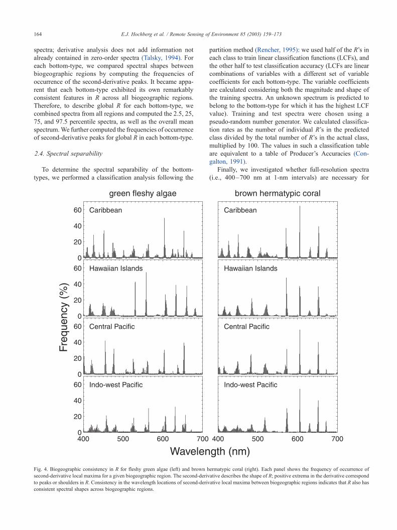
Fig. 4. Biogeographic consistency in R for fleshy green algae (left) and brown hermatypic coral (right). Each panel shows the frequency of occurrence of

second-derivative local maxima for a given biogeographic region. The second-derivative describes the shape of R; positive extrema in the derivative correspond

to peaks or shoulders in R. Consistency in the wavelength locations of second-derivative local maxima between biogeographic regions indicates that R also has

consistent spectral shapes across biogeographic regions.


spectral separation of the bottom-types. We used a multi-

variate stepwise selection procedure (Rencher, 1995) to find

the subset of wavelengths that best separates the 12 classes

(stepwise selection discards those wavelengths that are

statistically redundant for separating the bottom-types).

The selection produced a list of 52 wavelengths, which

appeared to aggregate in clusters of wavelengths. Conse-

quently, we further simplified the wavelength set by finding

the mean wavelength in each cluster, resulting in a 14-

wavelength list. We repeated the classification analysis

using the same training and test R’s, but undersampled to

the 52-wavelength and 14-wavelength sets.

3. Results

There are features in R that are common to all bottom-

types (Fig. 3). Low values at blue and green wavelengths are

largely the result of absorption by photosynthetic and photo-

protective compounds (Bidigare, Ondrusek, Morrow, &

Kiefer, 1990; Dove, Takabayashi, & Hoegh-Guldberg,

1995; Salih, Larkum, Cox, Kuhl, & Hoegh-Guldberg,

2000). Similarly, higher values at red wavelengths indicate

lack of absorption or presence of active fluorescence (Mazel,

1995). Chlorophyll absorption is readily apparent near 675

nm, and the effect of strong near-infrared reflectance is

apparent at 700 nm. Except for carbonate sand, all bottom-

types have low average R, generally falling in the range 0–

30%, and all have either peaks or shoulders near 600 and 650

nm. Finally, all bottom-types exhibit wide variations in the

magnitude of R, while maintaining the same relative shape.

In brown corals, R has the triple-peaked pattern described

by Hochberg and Atkinson (2000), which is marked by a

prominent positive reflectance feature near 570 nm (Fig. 3).

Healthy blue coral R is characterized by an absorption

feature (local minimum) near 580 nm and a plateau between

600 and 650 nm. The presence of fluorescent pigments

(Salih et al., 2000) in the coral tissue is sometimes apparent

as subtle positive features at blue and green wavelengths in

both healthy coral classes (though not apparent in Fig. 3).

The shape of bleached coral R resembles that of carbonate

sand more closely than that of either healthy coral class, but

the magnitude is intermediate between that of the healthy

corals and carbonate sand. Encrusting calcareous and turf

algae have spectral shapes similar to that of red fleshy algae.

These algae are characterized by two broad, positive fea-

tures in R over the ranges 435–490 and 500–565 nm.

Brown fleshy algae R also exhibits the first feature at 435–

490 nm, but lacks the second. Both green fleshy algae and

seagrass have a single broad reflectance feature centered at

550–560 nm. Soft/gorgonian coral R resembles that of

brown coral. Terrigenous mud is characterized by a very

low R, increasing nearly linearly from 1% at 400 nm to 8%

at 700 nm, and exhibiting a minimal chlorophyll absorption

feature near 675 nm. Finally, carbonate sand has a very high

R, with minimum values of 20% at 400 nm and reaching

maximum values of 80% at 700 nm.

In all bottom-types, locations of second-derivative peaks

are consistent across biogeographic regions. Fig. 4 is an

example showing fleshy green algae and brown hermatypic

coral. This consistency in peak location results from each

bottom-type having a suite of pigments that is conservative

throughout the world, and it is spectral absorption by these

pigments that ultimately determines the shape of R. Fig. 5

shows the frequencies of second-derivative peak wave-

lengths for all bottom-types across all biogeographic regions.

Fig. 5. Differences in spectral features between coral reef bottom-types. Each row corresponds to 1 of 12 bottom-types and shows the frequency of occurrence

of second-derivative local maxima across all biogeographic regions. Brighter grays (to white) indicate higher frequencies of occurrence (see color bar at

bottom). In each bottom-type, spectral features occur in tight wavelength bands, indicating worldwide consistency in R. All bottom-types exhibit features near

600 and 650 nm, while most differences between bottom-types occur at wavelengths V 570 nm. Notably, >90% of brown hermatypic corals and soft/gorgonian

corals have a feature near 570 nm, but all algal classes lack this feature.


Notably, brown hermatypic coral and soft/gorgonian coral

each have a strong feature near 570 nm, exhibited by no other

class. Nearly all peaks occur in narrow wavelength ranges,

sometimes as broad as 20 nm, but often on the order of 10 nm.

In the classification analysis, mean accuracy (average of

correct classification rates) was 83% (Table 1A) (we report

mean accuracy, rather than overall accuracy, due to the wide

differences in samples sizes between classes). In all instan-

ces of significant confusion between two bottom-types

(arbitrarily defined as a misclassification rate z 10%), the

confusion was one-way. Soft/gorgonian corals were mis-

classified as brown coral, but the reverse was not true. Most

classification errors occurred within, not between, broader

bottom-types. That is, algae tend to be misclassified as other

algae, and corals tend to be misclassified as other corals.

The class with highest classification error is soft/gorgonian

coral, which tends to be misclassified as brown coral more

often than it is correctly classified. To a much lesser extent

(i.e., < 10%), two-way misclassification occurs between

seagrass and fleshy green algae.

Table 1

Classification rates (%) for 12 basic coral reef bottom-types using in situ R with different waveband sets: full-resolution (301-wavelength at 1-nm intervals), 52-

wavelength, 14-wavelength

Predicted class

Algae Coral Other Sediment

Fleshy Non-fleshy Bleached Blue Brown Soft coral Seagrass Mud Sand

Brown Green Red Coralline Turf

(A) Full-resolution (400–700 nm at 1-nm intervals)

Actual class Algae fleshy brown 92.4 0.0 1.3 2.5 2.4 0.4 0.0 0.0 0.0 0.1 0.7 0.0

green 4.7 81.3 2.2 0.4 4.7 0.0 0.0 0.2 0.0 6.3 0.4 0.0

red 7.4 0.0 85.7 4.4 1.3 0.0 0.0 0.9 0.0 0.2 0.0 0.0

non-fleshy coralline 14.6 0.2 1.7 70.6 9.8 0.0 0.0 0.0 0.0 0.0 3.1 0.0

turf 12.7 0.9 2.3 6.8 73.5 1.1 0.0 0.0 0.0 2.0 0.7 0.0

Coral bleached 3.8 0.0 0.0 0.0 0.0 96.2 0.0 0.0 0.0 0.0 0.0 0.0

blue 0.0 0.4 3.3 0.0 0.0 0.0 72.3 23.1 0.0 0.0 0.8 0.0

brown 0.9 0.0 2.0 0.1 0.3 0.0 0.4 93.4 2.2 0.0 0.5 0.0

Other soft coral 1.1 0.0 0.0 0.0 0.0 0.0 0.0 52.1 43.6 0.0 3.2 0.0

seagrass 0.8 5.3 0.0 0.0 4.6 0.0 0.0 0.0 0.0 88.5 0.8 0.0

Sediment mud 0.0 0.0 0.0 0.0 0.0 0.0 0.0 0.0 0.0 0.0 100.0 0.0

sand 0.0 0.0 0.0 0.0 0.0 0.3 0.0 0.0 0.0 0.0 0.0 99.7

(B) 52-wavelength


green 6.3 75.0 1.3 2.5 2.9 0.2 0.0 0.0 0.0 9.9 2.0 0.0

red 6.7 0.0 85.2 5.4 1.1 0.0 0.0 1.1 0.0 0.0 0.6 0.0


turf 10.2 0.5 5.6 9.5 69.0 2.5 0.0 0.0 0.0 2.2 0.5 0.0

Coral bleached 0.0 0.0 0.0 0.0 19.2 80.8 0.0 0.0 0.0 0.0 0.0 0.0

blue 0.0 0.0 5.8 0.0 0.0 0.0 69.0 25.2 0.0 0.0 0.0 0.0

brown 0.2 0.0 4.7 0.0 0.3 0.2 0.6 90.7 1.9 0.0 1.2 0.0

Other soft coral 0.0 0.0 0.0 0.0 0.0 0.0 0.0 59.6 38.3 0.0 2.1 0.0

seagrass 0.8 17.6 0.0 0.0 6.9 0.0 0.0 0.0 0.0 74.0 0.8 0.0

Sediment mud 0.0 0.0 0.0 0.0 0.0 0.2 0.0 0.0 0.0 0.0 99.8 0.0

sand 0.0 0.0 0.0 0.0 0.0 0.3 0.0 0.0 0.0 0.0 0.0 99.7

(C) 14-wavelength


green 5.4 72.9 8.8 0.5 1.4 0.0 0.0 0.9 0.2 8.8 1.1 0.0

red 1.1 0.0 85.0 7.8 0.2 1.5 0.0 3.1 0.0 0.2 1.1 0.0


turf 10.4 0.0 2.2 15.1 59.9 5.7 0.0 1.1 0.0 2.7 3.0 0.0

Coral bleached 3.8 0.0 0.0 0.0 7.7 80.8 0.0 3.8 3.8 0.0 0.0 0.0

blue 0.0 0.0 3.7 0.0 0.0 0.0 69.8 26.0 0.0 0.0 0.4 0.0

brown 0.6 0.0 8.4 0.2 0.0 0.8 1.0 80.8 7.0 0.0 1.0 0.0

Other soft coral 0.0 0.0 0.0 0.0 0.0 0.0 0.0 60.6 39.4 0.0 0.0 0.0

seagrass 1.5 34.4 0.0 0.8 5.3 0.0 0.0 0.0 0.0 58.0 0.0 0.0

Sediment mud 0.0 0.0 0.0 0.0 0.0 0.4 0.0 0.0 0.0 0.0 99.6 0.0

sand 0.0 0.0 0.0 0.0 0.0 0.6 0.0 0.0 0.0 0.0 0.0 99.4

Classification rates are the number of individual R’s in the predicted class divided by the total number of R’s in the actual class, multiplied by 100. Diagonal

elements (in bold) represent correct classification rates, and off-diagonal elements represent misclassification rates. Misclassification rates z 10% are italicized.

Predicted classification rates (i.e., rows) sum to 100% (or near to 100% due to roundoff error).


The same patterns are present in both the 52-wavelength

and 14-wavelength classification rates (Table 1B and C).

Generally, with fewer wavelengths, misclassification rates

increase. Mean classification accuracy is 76% and 71% for

the 52-wavelength and 14-wavelength cases, respectively.

Table 2 lists the 52- and 14-wavelength sets used in the

subset analyses.

4. Discussion

R as reported here is a combination of the light flux not

absorbed by the bottom-types and the light fluoresced by the

bottom-types. Coral and zooxanthellae (unicellular algae

living endosymbiotically within coral-host tissue) pigments

have been shown to fluoresce (Dove, Hoegh-Guldberg, &

Ranganathan, 2001, Dove et al., 1995; Mazel, 1995, 1996;

Myers et al., 1999; Salih et al., 2000), and our data have

indications of that fluorescence. However, it is largely

spectral absorption by pigments that determines the overall

spectral shape of R. We demonstrate this by performing a

simple modeling exercise: we create a relative absorption

spectrum for brown coral (Fig. 6A) by summing the absorp-

tion spectra of five zooxanthellae pigments (chlorophyll a,

chlorophyll c, h-carotene, diadinoxanthin, peridinin), which

Fig. 6. Model of relative reflectance for brown coral using absorption spectra weighted by relative concentrations reported in literature. See text for details of

calculations. (A) Relative spectral absorptions by the five pigments in the model, and the total relative absorption. chl a= chlorophyll a, chl c= chlorophyll c, h-car =h-carotene, diadin = diadinoxanthin, per = peridinin. (B) Normalized reflectance for modeled and measured coral spectra. (C) Second derivative of (B).

Table 2

The 52- and 14-wavelength subsets used in classification analyses

52-wavelength subset 14-wavelength subset

400, 401, 405, 406, 407, 409, 411, 417,

420, 421, 427, 429, 431, 434, 438, 441,

445, 451, 455, 457, 466, 470, 481, 497,

499, 508, 509, 528, 540, 541, 559, 565,

571, 576, 579, 585, 599, 601, 609, 611,

629, 639, 644, 651, 666, 670, 678, 679,

685, 686, 689, 700

406, 430, 454, 467, 480,

499, 507, 529, 540, 577,

602, 608, 643, 684

The 52-wavelength subset was identified by multivariate stepwise selection

as those wavelengths that, without redundancy, provide greatest separation

of the 12 bottom-types. The 14-wavelength subset was identified inter-

actively as average wavelengths of clusters from 52-wavelength subset.

Wavelengths listed in nanometers.


have been weighted by their relative concentrations in corals,

as reported in the literature (Andersen, Bidigare, Keller, &

Latasa, 1996; Cottone, 1995; Fang, Liao, & Liu, 1995;

Kleppel, Dodge, & Reese, 1989; Myers et al., 1999). We

convert to relative reflectance by taking the base-10 loga-

rithm of the inverse of relative absorption (Talsky, 1994),

then normalizing by the result’s vector length. For compar-

ison, we average 4308 brown coral R’s and normalize that

spectrum by its vector length. The normalized spectra (Fig.

6B) are relative (as opposed to absolute) reflectances and

represent spectral shape independent of magnitude. The

modeled and in situ spectra compare favorably, each show-

ing the same triple-peaked pattern characteristic of brown

corals. Comparison of the second derivatives of the relative

reflectances confirms that both spectra have the same basic

shape (Fig. 6C). Furthermore, the R we have measured for

brown coral (and soft/gorgonian corals) is the inverse pattern

of spectral absorption by peridinin-containing dinoflagel-

lates (Johnsen, Samset, Granskog, & Sakshaug, 1994), the

group to which zooxanthellae belong. Thus, we conclude

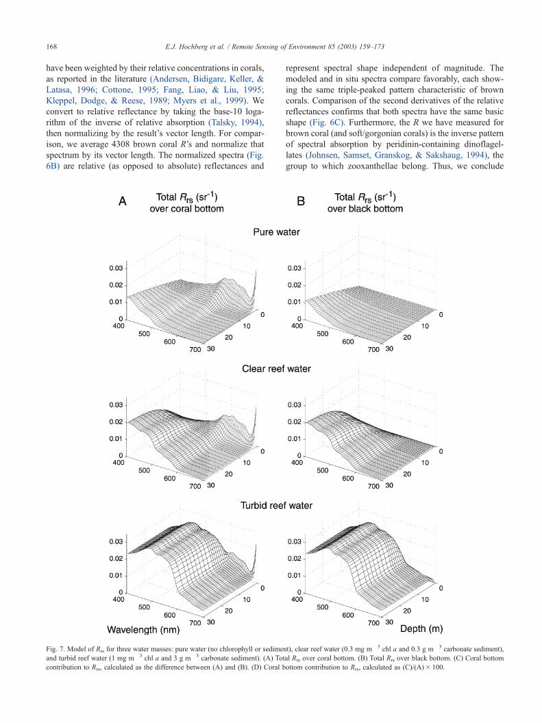
Fig. 7. Model of Rrs for three water masses: pure water (no chlorophyll or sediment), clear reef water (0.3 mg m� 3 chl a and 0.3 g m� 3 carbonate sediment),

and turbid reef water (1 mg m� 3 chl a and 3 g m� 3 carbonate sediment). (A) Total Rrs over coral bottom. (B) Total Rrs over black bottom. (C) Coral bottom

contribution to Rrs, calculated as the difference between (A) and (B). (D) Coral bottom contribution to Rrs, calculated as (C)/(A)� 100.


that, while fluorescence does contribute to R in specific

cases, the shape of R for brown coral is primarily determined

by zooxanthellae pigment absorption.

The concept that absorption is the primary determinant of

R can be extended to other reef bottom-types. For example,

the absorption feature near 580 nm in blue corals indicates

the presence of pocilloporin in the coral host (Dove et al.,

1995). Thus, R in blue corals results from a combination of

absorptions by zooxanthellae and host pigments. Encrusting

calcareous algae, turf algae, and red fleshy algae exhibit

similar R’s because the dominant (or sole) components of

these bottom-types all belong to the taxonomic division

Rhodophyta and therefore share the same suite of absorbing

pigments. Bleached coral has R similar to that of carbonate

sand due to loss of zooxanthellae combined with a decrease

in zooxanthellar and host pigmentation, resulting in optical

exposure of the coral carbonate skeleton (Kleppel et al.,

1989). Finally, R for carbonate sand itself shows the com-

bined effects of absorption by calcium carbonate sand grains

and chlorophyll in benthic microalgae (Roelfsema, Phinn, &

Dennison, 2002).

The fact that absorption by pigments is responsible for

the shape of R in reef bottom-types is expected. The same

principle has been the basis for remote sensing of ocean

Fig. 7 (continued).


color for more than 20 years (Gordon & Clark, 1980; Morel

& Prieur, 1977). It has been demonstrated that there is a link

between induced fluorescence of reef benthic organisms and

their pigment compositions and concentrations (Hardy,

Hodge, Yungel, & Dodge, 1992; Myers et al., 1999). Based

on those studies and our results, it may now be appropriate

to develop the field of ‘‘coral reef color.’’

We have presented Fig. 4 as a qualitative example show-

ing that the shape of R is geographically invariant. Unfortu-

nately, we cannot statistically explore this issue, since,

despite our large sample size, we do not have sufficient

numbers of measurements for each bottom-type in each

biogeographic region for appropriate multivariate tests (Ren-

cher, 1995). However, the peaks of second-derivative spectra

are consistent between regions (e.g., Fig. 4), which indicates

that the shapes of zero-order R are also consistent (Talsky,

1994). Geographic invariance in R is attributable to the facts

that (1) absorption is a fundamental process that is independ-

ent of biogeography and (2) the pigments responsible for

absorption also exist independently of biogeography. Geo-

graphic invariance of R within bottom-types has a corollary:

differences between bottom-types are also geographically

invariant. This is the biooptical basis for the spectral sepa-

ration achieved here through classification analysis.

Previous studies have demonstrated the feasibility of

using high-resolution remote sensing to assess coral reef

status (e.g., percent of live and dead corals) in localized

settings using extensive ground-truthing and unsupervised

classifications (e.g., Mumby, Chisolm, Clark, Hedley, &

Jaubert, 2001), but generalizations of methods have not

been possible. For example, the results obtained by Mumby

et al. (2001) at Rangiroa (Tuamotu Archipelago, French

Polynesia) are not reproducible at nearby Moorea (Society

Islands, French Polynesia), even using data from the same

hyperspectral imaging system, due to the influence of fleshy

brown algae at Moorea (Andrefouet, unpublished data;

Mumby, personal communication). That R for a given

bottom-type has the same shape regardless of geography

ultimately provides the foundation for development of

global discrimination/classification algorithms.

It is important to note that R is a convolution of

magnitude and relative shape, and both components con-

tribute to spectral separation between the bottom-types. An

example is the comparison between carbonate sand and

bleached coral: both bottom-types exhibit the same relative

spectral shape, because the dominant optically absorbing

component in each is the mineral calcium carbonate. How-

ever, carbonate sand has much higher overall reflectance

because bleached coral (1) actually retains some pigmenta-

tion in the zooxanthellae and coral host and (2) maintains its

three-dimensional structure which creates shadows, while

(3) the benthic microalgal community resident on sand

generates a smaller pigment absorption signature than that

of bleached coral, and (4) sand has a more two-dimensional

structure. More subtly, several of the bottom-types share

many second-derivative features (e.g., fleshy red algae and

non-fleshy turf algae), but do exhibit slight differences in

both the wavelengths at which the features occur (Fig. 5)

and their absolute magnitudes (Fig. 3). The implication is

that discrimination of bottom-types based on these subtle

spectral differences requires relatively high spectral resolu-

tion, with maximum bandwidths on the order of 10–20 nm.

For each of the three different wavelength sets used in the

classification analysis, the greatest occurrence of error is

soft/gorgonian coral misclassified as brown hermatypic

coral. In a region where soft/gorgonian corals are common

(e.g., many sites in the Caribbean), a remote sensing study

that considers only spectral variables may produce signifi-

cant overestimates of hermatypic coral cover. For many of

the world’s reefs, however, soft/gorgonian corals are not a

dominant benthic component and often occupy different reef

zones than hermatypic corals (Fabricius & Alderslade,

2001). Thus, an applied remote sensing study should also

make use of knowledge-based algorithms, employing eco-

logical (i.e., spatial) as well as spectral variables (e.g.,

Andrefouet & Roux, 1998).

Our results represent an upper limit to spectral classifica-

tion accuracy, because in situ R is independent of absorption

and scattering within the atmosphere and water column.

These radiative transfer processes spectrally alter the reef-

surface signal before it is received by the remote sensor, and

continued research is necessary to develop methods for

inverting their effects. One important factor that has yet to

be explored in detail (except seeMaritorena et al., 1994) is the

depth at which the bottom is no longer detectable. Consider-

ing only the water column and seafloor, this depth-of-detec-

tion limit (zlim) is a function of R and of the water column’s

optical properties. Because both R and water column optical

properties are functions of wavelength, so is zlim. We have

explored the behavior of zlim with respect to water column

optical properties using the radiative transfer model Hydro-

light 4.1 (C.D. Mobley and L.K. Sundman, Sequoia Scien-

tific, Redmond, WA, USA). We use a four-component model

(pure water, chlorophyll-bearing particles, colored dissolved

organic matter covarying with chlorophyll, and suspended

calcareous sediment) to simulate remote sensing reflectance

(Rrs, water-leaving radiance divided by downwelling irradi-

ance) for three water masses: pure water (no chlorophyll or

sediment), clear reef water (0.3 mg m� 3 chl a and 0.3 g m� 3

carbonate sediment), and turbid reef water (1 mg m� 3 chl a

and 3 g m� 3 carbonate sediment). We execute the model for

water depths in the range 0–30 m with the bottom boundary

specified as a coral bottom (our average brown coral spec-

trum, Fig. 7A) and as a perfectly absorbing bottom (flat

spectrum of 0% reflectance across all wavelengths, Fig. 7B).

Rrs over a coral bottom is comprised of a bottom component

and a water column component, whileRrs over a black bottom

expresses only the water column component (Maritorena et

al., 1994). By subtracting the latter from the former, we

estimate the contribution of the coral bottom to total Rrs (Fig.

7C), and by dividing this value by totalRrs andmultiplying by

100, we obtain the coral bottom contribution to total Rrs as a


percent (Fig. 7D). This value represents the relative signal-to-

noise level for the coral bottom, where noise is the water

column contribution to Rrs.

Fig. 8 shows the coral 5% and 10% signal levels as

functions of wavelength for the three water masses. In theory,

these lines are exact; we choose not to draw the 0% signal line

because, in practice, a radiometer pointed downward at a reef

will have difficulty resolving lower signal levels (i.e., sensor

signal-to-noise issues). Thus, these lines approximate func-

tional zlim. It is no surprise that zlim is much shallower for

turbid water than for clear water. It also should be noted that

most reef areas of interest in studies of community structure

lie well within the clear reef water zlim and that reef waters,

especially outer reef slopes, are often more clear than our

clear reef water case. Finally, these results are generally valid

for all the bottom-types except carbonate sand, because all

have roughly the same magnitude R as brown coral.

The wavelength dependence of zlim in clear reef water

indicates that remote sensing of coral reefs is best achieved at

wavelengths shorter than about 580 nm. This of course results

from the rapid rise in attenuation at longer wavelengths due to

absorption by water. There is potential for this effect to

interfere with remote discrimination of reef bottom-types:

the characteristic 570 nm feature in R of brown hermatypic

coral is at the cusp of increasing attenuation, and the attenu-

ation feature tends to produce a strong shoulder in Rrs in this

wavelength region for all water clarities and all bottom

compositions. The strength of the effect and the depth at

which it becomes apparent vary with water clarity. As long as

the bottom is not past zlim, however, there is potential for

inverse radiative transfer modeling to remove the effect, thus

allowing accurate identification of bottom-type.

With regard to the specific classification technique, we

have achieved high classification accuracy rates with simple

LCFs. With further tuning of our classifiers, it is possible to

achieve even higher levels of accuracy. More sophisticated

classifiers such as quadratic classification functions or multi-

variate density estimators will likely increase classification

accuracy of the ‘‘pure’’ bottom-type spectra, and others may

afford the ability to deconvolve spectrally mixed signals.

LCFs with full 1-nm-resolution spectra (i.e., 301 contig-

uous wavelengths) demonstrate high spectral separability of

the classes. Existing satellite sensors, however, do not

approach this degree of spectral resolution, and this fact

limits their abilities to discriminate between the 12 bottom-

types that we have defined. A repeat of our classification

analysis using appropriate sensor wavebands resulted in

mean classification accuracies of 41%, 45%, and 47% for

the satellite sensors SPOT-HRV (Systeme Pour l’Observa-

tion de la Terre—High Resolution Visible), Ikonos and

Landsat-ETM+ (Enhanced Thematic Mapper Plus), respec-

tively. At 78%, only the airborne sensor AVIRIS (Airborne

Visible Infrared Imaging Spectrometer, visible wavebands

only) has a mean classification accuracy commensurate with

that of full-resolution spectra. Fortuitously, in the near future,

satellite sensors will begin to match the spectral capabilities

of AVIRIS.

Alternatively, advancing technology has made it feasible

to design a satellite sensor with the purpose of addressing

specific questions in global coral reef science. Such a sensor

would possess particular wavebands explicitly chosen for the

task at hand, and it is important to determine classification

accuracies for these more realistic waveband sets. For

classification of the three more general bottom-types—algae,

coral, and sand—LCFs using four 20-nm-wide wavebands

achieved an overall accuracy of 91% (Hochberg & Atkinson,

2003). Coupling this waveband set with radiative transfer

models indicates that this spectral separation is achievable to

Fig. 8. Functional depth-of-detection limits (zlim) for the three water masses. Below zlim, inverse radiative transfer calculations are unable to reconstruct bottom

reflectance signatures. At a given wavelength, zlim is a function of water clarity and magnitude of bottom reflectance. These cases of zlim are computed for the

brown hermatypic coral bottom in Fig. 7D, but these results are extendable to other bottom-types, because most have R at approximately the same order of

magnitude as coral.


water depths between 5 and 10 m under a clean tropical

atmosphere and case 1 ocean water (Atkinson et al., 2001).

This demonstrates the utility of employing characteristic R as

the basis for space-borne coral reef remote sensing. Such

simplified waveband combinations ease satellite engineering

constraints (i.e., a sensor with fewer wavebands is easier to

design and operate), facilitating lower cost remote sensing

solutions to the problem of global coral reef study and

monitoring.

We have found measurement of R for any bottom-type to

be extremely repeatable. The R’s we have measured are

consistent in shape and magnitude with those reported by

other researchers using a similar methodology: near-simul-

taneous measurement of incident and reflected light fluxes

(Andrefouet et al., 2001; Clark et al., 2000; Hochberg &

Atkinson, 2000; Holden & LeDrew, 1998, 1999; Joyce &

Phinn, 2002; Lubin, Li, Sustan, Mazel, & Stamnes, 2001;

Maritorena et al., 1994; Miyazaki & Harashima, 1993;

Myers et al., 1999). We have shown that basic reef

bottom-types have characteristic R, that within each bot-

tom-type, the shape of R is consistent across biogeographic

regions, and that the bottom-types are spectrally separable

from each other. Our results provide the basis for other

research efforts aimed at detailed ecological interpretation of

global coral reef remote sensing imagery. Given that coral

reefs around the world are believed to be in peril, and that

current in situ sampling methods are incapable of providing

the synoptic information required for assessment of the

world’s coral reef resources, the need for a reef-monitoring

satellite is now greater than ever.

Acknowledgements

We are grateful for field assistance from Shannon

Atkinson, Mark Carmichael, Steve Dollar, Jim Falter, Jim

Fleming, Michael Guidry, Mika Hochberg, Brian Lapointe,

Jennifer Liebeler, Claude Payri, Russell Perkins, Brendalee

Phillips, Michel Pichon, Ann Tarrant, Bernard Thomassin,

and Robert Tomasetti. Logistical support for field operations

was provided by the US NOAA/NOS Biogeography

Program, the US National Park Service, and the US

Geological Survey. Our most effusive gratitude goes to

S.V. Smith for his comments and suggestions. This work

was funded by NASA award numbers NAG5-7513, NAG5-

5276 and NAG5-10908, and NOAA award number NA07-

OA0571. This is SOEST contribution 6053, HIMB

contribution 1147, and IMaRS contribution 0041.

References

Andersen, R., Bidigare, R., Keller, M., & Latasa, M. (1996). A comparison

of HPLC pigment signatures and electron microscopic observations for

oligotrophic waters of the North Atlantic and Pacific Oceans. Deep-Sea

Research II, 43, 517–537.

Andrefouet, S., Muller-Karger, F. E., Hochberg, E. J., Hu, C., & Carder,

K. L. (2001). Change detection in shallow coral reef environments

using Landsat 7 ETM+ data. Remote Sensing of Environment, 79,

150–162.

Andrefouet, S., & Payri, C. (2001). Scaling-up carbon and carbonate me-

tabolism of coral reefs using in-situ data and remote sensing. Coral

Reefs, 19, 259–269.

Andrefouet, S., Robinson, J. A., Hu, C., Feldman, G. C., Salvat, B., Payri,

C., & Muller-Karger, F. E. (2003). Influence of the spatial resolution of

SeaWiFS, Landsat 7, SPOT and International Space Station data on

estimates of landscape parameters of Pacific Ocean atolls. Canadian

Journal of Remote Sensing, 29 (No. 2).

Andrefouet, S., & Roux, L. (1998). Characterisation of ecotones using

membership degrees computed with a fuzzy classifier. International

Journal of Remote Sensing, 19, 3205–3211.

Atkinson, M. J., Lucey, P. G., Taylor, G. J., Porter, J., Dollar, S., & An-

drefouet, S. (2001). CRESPO: Coral Reef Ecosystem Spectro-Photo-

metric Observatory, concept study report to the University Earth

System Science Program, National Aeronautics and Space Administra-

tion. Honolulu: University of Hawaii, 137 pp.

Bastidas, C., Benzie, J. A. H., Uthicke, S., & Fabricius, K. E. (2001).

Genetic differentiation among populations of a broadcast spawning soft

coral, Sinularia flexibilis, on the Great Barrier Reef. Marine Biology,

138, 517–525.

Ben-Yosef, D. Z., & Benayahu, Y. (1999). The gorgonian coral Acabaria

biseralis: life history of a successful colonizer of artificial substrata.

Marine Biology, 135, 473–481.

Berner, T. (1990). Coral-reef algae. In Z. Dubinsky (Ed.), Ecosystems of the

World 25: Coral Reefs ( pp. 253–264). Amsterdam: Elsevier.

Bidigare, R. R., Ondrusek, M. E., Morrow, J. H., & Kiefer, D. A. (1990). In

vivo absorption properties of algal pigments. Proceedings of Ocean

Optics X, SPIE vol. 1302 ( pp. 290–302). Orlando, FL: SPIE.

Buddemeier, R., & Smith, S. V. (1999). Coral adaptation and acclimatiza-

tion: a most ingenious paradox. American Zoologist, 39, 1–9.

Chabanet, P., Ralambondrainy, H., Amanieu, M., Faure, G., & Galzin, R.

(1997). Relationships between coral reef substrata and fish. Coral Reefs,

16, 93–102.

Clark, C. D., Mumby, P. J., Chisholm, J. R. M., Jaubert, J., & Andrefouet,

S. (2000). Spectral discrimination of coral mortality states following a

severe bleaching event. International Journal of Remote Sensing, 21,

2321–2327.

Congalton, R. G. (1991). A review of assessing the accuracy of classifi-

cations of remotely sensed data. Remote Sensing of Environment, 37,

35–46.

Connell, J. H. (1997). Disturbance and recovery of coral assemblages.

Coral Reefs, 16, S101–S113.

Cottone, M. C. (1995). Coral pigments: quantification using HPLC and

detection by remote sensing. Master’s Thesis, Western Washington Uni-

versity.

Done, T. J. (1992). Phase shifts in coral reef communities and their eco-

logical significance. Hydrobiologia, 247, 121–132.

Done, T. J. (1995). Ecological criteria for evaluating coral reefs and their

implications for managers and researchers. Coral Reefs, 14, 183–192.

Dove, S. G., Hoegh-Guldberg, O., & Ranganathan, S. (2001). Major colour

patterns of reef-building corals are due to a family of GFP-like proteins.

Coral Reefs, 19, 197–204.

Dove, S. G., Takabayashi, M., & Hoegh-Guldberg, O. (1995). Isolation and

partial characterization of the pink and blue pigments of Pocilloporid

and Acroporid corals. Biological Bulletin, 189, 288–297.

Enrıquez, S., Merino, M., & Iglesias-Prieto, R. (2002). Variations in the

photosynthetic performance along the leaves of the tropical seagrass

Thalassia testudinum. Marine Biology, 140, 891–900.

Fabricius, K. E. (1997). Soft coral abundance on the central Great Barrier

Reef: effects of Acanthaster planci, space availability, and aspects of the

physical environment. Coral Reefs, 16, 159–167.

Fabricius, K. E., & Alderslade, P. (2001). Soft corals and sea fans: a com-

prehensive guide to the tropical shallow-water genera of the Central-


West Pacific, the Indian Ocean and the Red Sea. Townsville, Queens-

land, Australia: Australian Institute of Marine Science, 264 pp.

Fang, L.-S., Liao, C.-W., & Liu, M.-C. (1995). Pigment composition in

different-colored scleractinian corals before and during the bleaching

process. Zoological Studies, 34, 10–17.

Ginsburg, R. N. (Ed.) (1994). Proceedings of the Colloquium on Global

Aspects of Coral Reefs: Health, Hazards and History. Miami: Rosenstiel

School of Marine and Atmospheric Sciences, University of Miami,

420 pp.

Glynn, P. W. (1990). Feeding ecology of coral-reef macroconsumers. In: Z.

Dubinsky (Ed.), Ecosystems of the world 25: coral reefs (pp. 365–400).

Amsterdam: Elsevier.

Gordon, H. R., & Clark, D. K. (1980). Atmospheric effects in the remote

sensing of phytoplankton pigments. Boundary-layer Meteorology, 18,

299–313.

Green, E. P., Mumby, P. J., Edwards, A. J., & Clark, C. D. (1996). A review

of remote sensing for the assessment and management of tropical coast-

al resources. Coastal Management, 24, 1–40.

Hardy, J. T., Hodge, F. E., Yungel, J. K., & Dodge, R. E. (1992). Remote

detection of coral ’bleaching’ using pulsed-laser fluorescence spectro-

scopy. Marine Ecology Progress Series, 88, 247–255.

Hedley, J. D., & Mumby, P. J. (2002). Biological and remote sensing

perspectives of pigmentation in coral reef organisms. In A. J. Young,

C. M. Young, & L. A. Fuiman (Eds.), Advances in Marine Biology, vol.

43 (pp. 279–317). San Diego: Academic Press.

Hochberg, E. J., & Atkinson, M. J. (2000). Spectral discrimination of coral

reef benthic communities. Coral Reefs, 19, 164–171.

Hochberg, E. J. & Atkinson, M. J. (2003). Capabilities of remote sensors to

classify coral, algae and sand as pure and mixed spectra. Remote Sens-

ing of Environment 85, 174–189 (this issue).

Holden, H., & LeDrew, E. (1998). Spectral discrimination of healthy and

non-healthy corals based on cluster analysis, principal components anal-

ysis, and derivative spectroscopy. Remote Sensing of Environment, 65,

217–224.

Holden, H., & LeDrew, E. (1999). Hyperspectral identification of coral reef

features. International Journal of Remote Sensing, 20, 2545–2563.

Johnsen, G., Samset, O., Granskog, L., & Sakshaug, E. (1994). In vivo

absorption characteristics in 10 classes of bloom-forming phytoplank-

ton: taxonomic characteristics and responses to photoadaptation by

means of discriminant and HPLC analysis. Marine Ecology Progress

Series, 105, 149–157.

Joyce, K. E., & Phinn, S. R. (2002). Bi-directional reflectance of corals.

International Journal of Remote Sensing, 23, 389–394.

Kinsey, D. W. (1985). Metabolism, calcification and carbon production I:

systems level studies. Fifth International Coral Reef Congress. Tahiti,

vol. 4 (pp. 505–526). Moorea, French, Polynesia: Antenne Museum-

EPHE.

Kirk, J. T. O. (1994). Light and photosynthesis in aquatic environments.

Cambridge: Cambridge Univ. Press, 509 pp.

Kleppel, G., Dodge, R., & Reese, C. (1989). Changes in pigmentation

associated with the bleaching of stony corals. Limnology and Ocean-

ography, 34, 1331–1335.

Klumpp, D. W., & McKinnon, A. D. (1989). Temporal and spatial patterns

in primary production of a coral-reef epilithic algal community. Journal

of Experimental Marine Biology and Ecology, 131, 1–22.

Light, P. R., & Jones, G. P. (1997). Habitat preference in newly settled coral

trout (Plectropomus leopardus, Serranidae). Coral Reefs, 16, 117–126.

Lubin, D., Li, W., Dustan, P., Mazel, C. H., & Stamnes, K. (2001). Spectral

signatures of coral reefs: features from space. Remote Sensing of Envi-

ronment, 75, 127–137.

Maritorena, S., Morel, A., & Gentili, B. (1994). Diffuse reflectance of

oceanic shallow waters: influence of water depth and bottom albedo.

Limnology and Oceanography, 39, 1689–1703.

Mazel, C. H. (1995). Spectral measurements of fluorescence emission in

Caribbean cnidarians. Marine Ecology Progress Series, 120, 185–191.

Mazel, C. H. (1996). Coral fluorescence characteristics: excitation-emission

spectra, fluorescence efficiencies, and contribution to apparent reflec-

tance. Proceedings of Ocean Optics XIII-SPIE vol. 2963, 1 (pp. 240–

245). Halifax, Nova Scotia, Canada: SPIE.

Miller, I., & Muller, R. (1999). Validity and reproducibility of benthic cover

estimates made during broadscale surveys of coral reefs by manta tow.


Miller, M. W., Weil, E., & Szmant, A. M. (2000). Coral recruitment and

juvenile mortality as structuring factors for reef benthic communities in

Biscayne National Park, USA. Coral Reefs, 19, 115–123.

Minghelli-Roman, A., Chisholm, J. R. M., Marchioretti, M., & Jaubert, J.

M. (2002). Discrimination of coral reflectance spectra in the Red Sea.


Miyazaki, T., & Harashima, A. (1993). Measuring the spectral signatures of

coral reefs. Thirteenth Annual International Geoscience and Remote

Sensing Symposium, vol. 2 ( pp. 693–695). Tokyo, Japan: IEEE.

Miyazaki, T., Nakatani, Y., & Harashima, A. (1995). Measuring the coral

reef distribution of Kuroshima Island by satellite remote sensing.

Proceedings of Global Process Monitoring and Remote Sensing of

the Ocean and Sea Ice-SPIE vol. 2586, 1 ( pp. 65–72). Paris, France:

SPIE.

Morel, A., & Prieur, L. (1977). Analysis of variations in ocean color.

Limnology and Oceanography, 22, 709–722.

Morel, A., & Smith, R. C. (1993). Terminology and units in optical ocean-

ography. US JGOFS Planning Report Number 18: Bio-Optics in US

JGOFS: 149–157.

Mumby, P. J., Chisolm, J. R. M., Clark, C. D., Hedley, J. D., & Jaubert, J.

(2001). A bird’s eye view of the health of coral reefs. Nature, 413, 36.

Mumby, P. J., & Edwards, A. J. (2002). Mapping marine environments

with IKONOS imagery: enhanced spatial resolution can deliver greater

thematic accuracy. Remote Sensing of Environment, 82, 248–257.

Mumby, P. J., Green, E. P., Clark, C. D., & Edwards, A. J. (1998). Digital

analysis of multispectral airborne imagery of coral reefs. Coral Reefs,

17, 59–69.

Mumby, P. J., Green, E. P., Edwards, A. J., & Clark, C. D. (1999). The

cost-effectiveness of remote sensing for tropical coastal resources as-

sessment and management. Journal of Environmental Management, 55,

157–166.

Myers, M. R., Hardy, J. T., Mazel, C. H., & Dustan, P. (1999). Optical

spectra and pigmentation of Caribbean reef corals and macroalgae.


Rencher, A. C. (1995).Methods of multivariate analysis. New York: Wiley,

627 pp.

Roelfsema, C. M., Phinn, S. R., & Dennison, W. C. (2002). Spatial dis-

tribution of benthic microalgae on coral reefs determined by remote

sensing. Coral Reefs, 21, 264–274.

Salih, A., Larkum, A., Cox, G., Kuhl, M., & Hoegh-Guldberg, O.

(2000). Fluorescent pigments in corals are photoprotective. Nature,

408, 850–853.

Savitsky, A., & Golay, M. J. E. (1964). Smoothing and differentiation of

data by simplified least squares procedures. Analytical Chemistry, 36,

1627–1639.

Steiner, J., Termonia, Y., & Deltour, J. (1972). Comments on smoothing

and differentiation of data by simplified least square procedure. Ana-

lytical Chemistry, 44, 1906–1909.

Stoddart, D. R. (1969). Ecology and morphology of recent coral reefs. Bio-

logical Reviews of the Cambridge Philosophical Society, 44, 433–498.

Talsky, G. (1994). Derivative spectrophotometry: low and high order. New

York: Weinheim, 228 pp.

Veron, J. E. N. (1995). Corals in space and time: the biogeography and

evolution of the Scleractinia. Ithaca: Cornell Univ. Press, 321 pp.

Watanabe, F., Nakamura, K., Samarakoon, L., Mabuchi, Y., & Ishibashi, A.

(1993). A procedure for estimating and monitoring red soil spread on

coral reefs of Okinawa using multitemporal Landsat TM data. 1993

Proceedings of the Thirteenth International Geoscience and Remote

Sensing Symposium, vol 2 (pp. 696–699). Tokyo, Japan: IEEE.

Wilkinson, C. (Ed.) (2000). Status of coral reefs of the world: 2000.

Townsville, Queensland, Australia: Australian Institute of Marine Sci-

ence, 363 pp.


Documents

Spectral reflectance of coral reef bottom-types worldwide and ...optics.marine.usf.edu/~hu/scratch/jpl_ref/Hochberg_RSE.pdf · Spectral reflectance of coral reef bottom-types worldwide