FEDERAL RESERVE BANK OF SAN FRANCISCO

WORKING PAPER SERIES

Working Paper 2008-08 http://www.frbsf.org/publications/economics/papers/2008/wp08-08bk.pdf

The views in this paper are solely the responsibility of the authors and should not be interpreted as reflecting the views of the Federal Reserve Bank of San Francisco or the Board of Governors of the Federal Reserve System.

Speculative Growth and Overreaction to Technology Shocks

Kevin J. Lansing Federal Reserve Bank of San Francisco

December 2008

Speculative Growth and Overreaction to Technology Shocks∗

Kevin J. Lansing†

Federal Reserve Bank of San Francisco

December 11, 2008

Abstract

This paper develops a stochastic endogenous growth model that exhibits “excess volatil-ity” of equity prices because speculative agents overreact to observed technology shocks.When making forecasts about the future, speculative agents behave like rational agentswith very low risk aversion. The speculative forecast rule alters the dynamics of the modelin a way that tends to confirm the stronger technology response. For moderate levels ofrisk aversion, the forecast errors observed by the speculative agent are close to white noise,making it difficult for the agent to detect a misspecification of the forecast rule. In modelsimulations, I show that this type of behavior gives rise to intermittent asset price bubblesthat coincide with improvements in technology, investment and consumption booms, andfaster trend growth, reminiscent of the U.S. economy during the late 1920s and late 1990s.The model can also generate prolonged periods where the price-dividend ratio remains inthe vicinity of the fundamental value. The welfare cost of speculation (relative to rationalbehavior) depends crucially on parameter values. Speculation can improve welfare if actualrisk aversion is low and agents underinvest relative to the socially-optimal level. But forhigher levels of risk aversion, the welfare cost of speculation is large, typically exceedingone percent of per-period consumption.

Keywords: Endogenous Growth, Business Cycles, Excess Volatility, Asset Pricing, Specu-lative Bubbles.

JEL Classification: E32, E44, G12, O40.

∗For helpful comments and suggestions, I thank Bill Gavin, Steve LeRoy, participants at the 2008 Symposiumof the Society for Nonlinear Dynamics and Econometrics, the 2008 Meeting of the Society for Computation inEconomics and Finance, the 2008 Dynare conference, and the Fall 2008 Fed Macro conference.

† Research Department, Federal Reserve Bank of San Francisco, P.O. Box 7702, San Francisco,CA 94120-7702, (415) 974-2393, FAX: (415) 977-4031, email: kevin.j.lansing@sf.frb.org, homepage:www.frbsf.org/economics/economists/klansing.html

Bubbles are often precipitated by perceptions of real improvements in the produc-tivity and underlying profitability of the corporate economy. But as history attests,investors then too often exaggerate the extent of the improvement in economic fun-damentals.Federal Reserve Chairman Alan Greenspan, August 30, 2002.

1 Introduction

The magnitude of short-term movements in stock prices remains a challenge to explain withina framework of rational, efficient markets. Numerous empirical studies starting with Shiller(1981) and LeRoy and Porter (1981) have shown that stock prices appear to exhibit “excessvolatility” when compared to the discounted stream of ex post realized dividends.1 Anotherprominent feature of stock price data is the intermittent occurrence of sustained run-ups aboveestimates of fundamental value, so-called speculative bubbles, that can be found throughouthistory in various countries and asset markets.2 The dramatic rise in U.S. stock prices duringthe late 1990s, followed similarly by U.S. house prices during the mid 2000s, are episodes thathave both been described as bubbles. The former episode was accompanied by a boom inbusiness investment, while the later was accompanied by a boom in residential investment.Both booms were later followed by falling asset prices and severe retrenchments in the associ-ated investment series, as agents sought to unwind the excess capital accumulated during thebubble periods. Coincident booms in stock prices and investment also occurred during thelate 1920’s–a period that shares many characteristics with the late 1990s. In particular, bothperiods witnessed major technological innovations that contributed to investor enthusiasmabout a “new era.”3

This paper develops a stochastic endogenous growth model that seeks to formalize theapparent link between speculative bubbles, technological innovation, and capital misalloca-tion. I introduce excess volatility by assuming that agents engage in a form of speculativebehavior that manifests itself by overreaction to observed technology shocks. When makingforecasts about the future, speculative agents behave like rational agents with very low riskaversion. This characterization of speculative behavior, while by no means exclusive, resem-bles Hirshleifer’s (1975, p. 519) description of “the Keynes-Hicks view, [where] speculatorsare characterized not by any special knowledge or beliefs, but simply by their willingness totolerate risks...” In this paper, speculative agents behave like overconfident gamblers whosebets (forecasts) are too risky relative to that of a player who seeks to maximize winnings(lifetime utility).4

1Shiller (2003) provides a recent update on this literature.2See the collection of papers in Hunter, Kaufman, and Pomerleano (2003) for an overview of historical bubble

episodes.3As described further below, the similarities between the two periods is noted by Shiller (2000), Gordon

(2006), and White (2006).4Harrison and Kreps (1978) employ a different characterization of speculation in a model that involves

heterogenous beliefs and an exogenous constraint on short sales. Speculative agents are defined as those who

1

The framework for the analysis is a real business cycle model with endogenous growthand capital adjustment costs, along the lines of Barlevy (2004). I allow for the possibilityof an Arrow-Romer type productive externality, such that agents may underinvest relative tothe socially-optimal level. The presence of the externality yields an endogenous separationbetween consumption and dividends, where consumption growth is less volatile than dividendgrowth, as in long-run U.S. data. The severity of the underinvestment problem turns out tobe important for analyzing the welfare consequences of fluctuations which, in this model, canaffect the economy’s trend growth rate.

Under rational expectations, the technology-response coefficient in the agent’s forecast ruleis small in magnitude, such that the equilibrium price-dividend ratio is nearly constant forreasonable levels of risk aversion. In contrast, the price-dividend ratio in long-run U.S. stockmarket data is volatile and highly persistent, i.e., close to a random walk. The model resultobtains because rational agents understand that technology shocks give rise to both incomeand substitution effects which work in opposite directions. The two effects exactly cancelwhen the coefficient of relative risk aversion is unity, representing logarithmic utility. In thiscase, the technology response coefficient in the rational forecast rule is zero, such that theequilibrium price-dividend ratio is constant.

In the speculation model, the agent’s forecast rule takes the same form as the rationalforecast, but it features a stronger technology response coefficient, generating overreaction. Icalibrate the technology response coefficient so that the model matches the volatility of theprice-dividend ratio in U.S. data. Given the calibration, I can recover the hypothetical riskcoefficient that makes the speculative agent’s response coefficient identical to that of a rationalagent with lower risk aversion. In this sense, the speculative agent can be viewed as makingbets about the future which are too risky relative to that of a rational agent. But, as discussedfurther below, speculative behavior may actually improve welfare for some parameterizationsof the model by helping to mitigate the economy’s underinvestment problem.

Due to the self-referential nature of the agent’s decision problem, the initial use of aspeculative forecast rule alters the dynamics of the model in a way that tends to confirmthe stronger technology response. Using a real time learning algorithm, I demonstrate thatconvergence to the rational solution can be very slow when the agent initially adopts a forecastrule that is characterized by overreaction. In the calibrated model, I show that the forecasterrors observed by the speculative agent are close to white noise for moderate levels of riskaversion, making it difficult for the agent to detect a misspecification of the forecast rule.Moreover, from the individual agent’s perspective, switching to a fundamentals-based forecastrule (which involve a weaker technology response) would appear to reduce forecast accuracy,so there is no incentive to switch.

The capital adjustment cost formulation in the model implies that movements in the equityprice are linked directly to movements in investment. Barro (1990) finds that changes in realstock prices since 1891 have strong explanatory power for the growth rate of business invest-

are willing to pay more than their estimate of fundamental value due to the prospect of reselling later at a higherprice. This form of speculation is employed in the models of Scheinkman and Xiong (2003) and Panageous(2005).

2

ment. Studies by Chirinko and Schaller (2001, 2007), Gilchrist et al. (2005), and Campelloand Graham (2007) all find evidence of a significant empirical link between stock price bubblesand investment decisions by firms.

In model simulations, speculative behavior gives rise to intermittent asset price bubblesthat coincide with positive innovations in technology, investment and consumption booms, andfaster trend growth, reminiscent of the U.S. economy during the late 1920s and late 1990s.The model can also generate prolonged periods where the price-dividend ratio remains in thevicinity of the fundamental value. Due to the nonlinear nature of the model solution, thesimulated price-dividend ratio exhibits non-Gaussian features, such as positive skewness andexcess kurtosis. These features are also present in the data.

Interestingly, the speculation model outperforms the rational model in matching the rel-ative volatilities of detrended consumption, investment, and output. The presence of capitaladjustment costs causes investment in the rational model to exhibit about the same volatilityas output, whereas investment in the data is more than twice as volatile as output. Barlevy(2004, p. 983) acknowledges the difficulty of generating sufficient investment volatility in arational model with capital adjustment costs. However, in the speculation model, the agent’soverreaction behavior magnifies investment volatility so that investment is about twice asvolatile as output, which is much closer to the data.

Finally, I examine the welfare costs of fluctuations that can be attributed to either: (i)speculative behavior, or (ii) business cycles. Welfare costs are measured by the percentagechange in per-period consumption that makes the agent indifferent between the two economiesbeing compared. The welfare cost of speculative behavior (relative to rational behavior) de-pends crucially on parameter values. Speculation can improve welfare if actual risk aversionis low and agents underinvest relative to the socially-optimal level. But for higher levels ofrisk aversion, the welfare cost of speculation is large, typically exceeding one percent of con-sumption. Similarly, the welfare cost of business cycle fluctuations in the speculation model(relative to a deterministic model) increase rapidly with risk aversion.

The welfare results involve a complex interaction of several effects. Fluctuations in themodel can affect both the mean and volatility of consumption growth. If fluctuations decreasemean growth, then a smaller fraction of resources will be devoted to investment. Less in-vestment implies a higher initial level of consumption which, as noted by Barlevy (2004), canmitigate the negative effects of slower growth. But if the economy is subject to an underin-vestment problem, then higher initial consumption is less desirable. Finally, as the curvatureof the utility function increases, consumption growth volatility becomes more costly in termsof welfare. Which of these effects dominate depends on parameter values.

An important unsettled question in economics is whether policymakers should take delib-erate steps to prevent or deflate asset price bubbles.5 Those who advocate leaning againstbubbles point out that excessive asset prices can distort economic and financial decisions, cre-ating costly misallocations that can take years to dissipate. Others argue that policies intendedto prick a suspected bubble would likely send the economy into a recession, thereby foregoing

5For an overview of this literature, see Lansing (2008).

3

the benefits of the boom that might otherwise continue. The welfare results obtained hereprovide some support for both points of view.

1.1 Related Literature

The term “excess volatility” implies that asset prices move too much to be explained bychanges in dividends or cash flows. The behavioral finance literature has examined a widevariety of evidence pertaining to this phenomenon. Controlled experiments on human sub-jects suggest that people’s decisions are influenced by various “heuristics,” as documented byTversky and Kahneman (1974). The “representativeness heuristic” is a form of non-Bayesianupdating whereby subjects tend to overweight recent observations relative to the underlyinglaws of probability that govern the stochastic process. De Bondt and Thaler (1985) find evi-dence of overreaction in comparing returns of portfolios comprised of prior winning and losingstocks. Arbarbanell and Bernard (1992) and Easterwood and Nutt (1999) find evidence thatsecurity analysts’ earnings forecasts tend to overreact to new information, particularly whenthe information is positive in nature. Daniel, et al. (1998) develop a model where investors’overconfidence about the precision of certain types of information causes them to overreact tothat information. In the laboratory asset market of Caginalp et al. (2000), prices appeared tooverreact to fundamentals and to be driven by previous price changes, i.e., momentum.

This paper relates to a long list of research that explores the links between non-fundamentalasset price movements and investment in physical capital. Theoretical research that examinesrational bubbles in overlapping generations models with productive externalities or marketimperfections includes Saint Paul (1992), Grossman and Yanagawa (1993), King and Ferguson(1993), Oliver (2000), and Caballero et al. (2006).6 Unlike these papers, the bubbles exploredhere are driven by agents’ excessively risky bets about the future. Moreover, I use a calibratedversion of the model to compute the welfare costs of the capital misallocation that results fromthis behavior.

Dupor (2002, 2005) examines the policy implications of non-fundamental asset price move-ments in monetary real business cycle model with capital adjustments costs. Non-fundamentalasset price movements are driven by exogenous “expectation shocks” that a drive a wedge be-tween the true marginal product of capital and the market return observed by firms whenmaking their investment decisions. The volatility of these shocks is calibrated to match areturn volatility statistic for the S&P 500 index, analogous to the procedure used here tocalibrate the agent’s technology response coefficient. He finds that optimal monetary policyshould lean against non-fundamental asset price movements.

Jaimovich and Rebelo (2007) examine a behavioral real business cycle model that allowsfor non-rational expectations. In one version, agents are overconfident about the precision ofnews about future technology innovations, which causes them to overreact to that news, asin the model of Daniel, et al. (1998). The agents’ behavior serves to amplify the responseof investment to technology shocks. The authors do not examine the resulting welfare costs,however.

6Barlevy (2007, pp. 54-55) provides an overview of this literature.

4

In a recent paper, Hassan and Mertens (2008) consider the welfare costs of excess volatilityin a capitalist-worker model where the forecasts of capital owners are perturbed away from therational expectation by an exogenous shock, similar to the model of Dupor (2002, 2005). Theyfind that the welfare cost of excess volatility can be quite high (on the order of 4 percent ofper-period consumption) because volatility depresses the steady state capital stock and hencethe wages of workers.

The approach taken here is to postulate a particular form of less-than-rational behavior(overreaction) and then explore the economic consequences in a standard model. Other assetpricing research along these lines includes: Delong et al. (1990), Barsky and Delong (1993),Timmerman (1996), Barberis, Schleifer, and Vishney (1998), Brock and Hommes (1998), Cec-chetti, Lam, and Mark (2000), Abel (2002), Abreu and Brunnermeier (2003), Scheinkmanand Xiong (2003), Panageous (2005), Lansing (2006, 2007), and Adam, Marcet, and Nicolini(2008), among others.

Numerous papers seek to account for the behavior of the stock market or investment usingrational models where agents respond optimally to fundamental uncertainty about the futuretrend growth rate or the future level/profitability of technology. Research along these linesincludes Zeira (1999), Greenwood and Jovanovic (1999), Hobijn and Jovanovic (2001), Pástorand Veronesi (2006), Jermann and Quadrini (2007), Johnson (2007), Christiano et al. (2007),and Angeletos, Lorenzoni, and Pavan (2007).

Finally, McGrattan and Prescott (2007) acknowledge that the basic neoclassical growthmodel with rational expectations cannot account for the boom in U.S. business investmentthat occurred during the late 1990s. Along the lines of Hall (2001), they argue that accountingfor investment in intangible capital helps to reconcile the model with the data.

2 Historical Motivation

The basic premise of the paper is that investors overreact to technological change. A readingof stock market history lends support to this view. Shiller (2000) argues that major stock pricerun-ups have generally coincided with the emergence of some superficially-plausible “new era”theory that involves the introduction of new technology. Figure 1 depicts four major run-ups in real U.S. stock prices.7 Shiller associates each run-up with the following technologicaladvances that contributed to new era enthusiasm:

• Early 1900s: High-speed rail travel, transatlantic radio, long-line electrical transmission.

• 1920s: Mass production of automobiles, travel by highways and roads, commercial radiobroadcasts, widespread electrification of manufacturing.

• 1950s and 60s: Widespread introduction of television, advent of the suburban lifestyle,space travel.

7All data on stock prices, dividends, and consumption in the paper are from Robert Shiller’s website:http://www.econ.yale.edu/~shiller/.

5

• Late 1990s: Widespread availability of the internet, innovations in computers and infor-mation technology, emergence of the web-based business model.

In comparing the late 1920s with the late 1990s, Gordon (2006) and White (2006) both em-phasize the simultaneous occurrence of major technological innovations, a productivity revival,excess capital investment, and a stock market bubble fueled by speculation. Schwert (1989,2002) documents the pronounced increase in stock market volatility that occurred during bothperiods, particularly in technology-related stocks in the late 1990s. Cooper et al. (2001) doc-ument a pronounced “dotcom effect” in the late 1990s, whereby internet-related corporatename changes produced permanent abnormal returns. The authors attribute their results toa form a speculative mania among investors for “glamour” industries that are associated withnew technology.

The September 7, 1929 edition of Business Week famously remarked “For 5 years at least,American business has been in the grip of an apocalyptic holy-rolling exaltation over the un-paralleled prosperity of the ‘new era’ upon which we, or it, or somebody has entered.” TheMarch 8, 1999 cover story of Business Week proclaimed “The high-tech industry is on thecusp of a new era in computing in which digital smarts won’t be tied up in a mainframe, mini-computer, or PC. Instead, computing will come in a vast array of devices aimed at practicallyevery aspect of our daily lives.” Figure 2 illustrates the similarity of the stock price movementsthat took place during the two periods.

From 1996 until its peak in 2000 real business investment expanded at an average com-pound growth rate of 10 percent per year–about 2.5 times faster than the growth rate of theU.S. economy as a whole. Much of the surge in business investment in the late 1990s waslinked to computers and information technology. During these years, measured productivitygrowth picked up, which was often cited as evidence of a permanent structural change–onethat portended faster trend growth going forward.8 Widespread belief in the so-called “neweconomy” caused investors to bid up stock prices to unprecedented levels relative to dividends(Figure 3). The rise and fall of potential output growth (a proxy for the new economy’s speedlimit) coincides roughly with cyclical movements in the stock market (Figure 4). This mo-tivates consideration of a model where speculative behavior can affect the economy’s trendgrowth rate.

The investment boom of the late 1990s now appears to have been overdone. Firms overin-vested in new productive capacity in an effort to satisfy a level of demand for their productsthat proved to be unsustainable.9 Caballero et al. (2006) argue that rapidly rising stock pricesprovided firms with a low-cost source of funds from which to finance their investment projects.The resulting surge in capital accumulation served to increase measured productivity growth

8For an optimistic assessment at the time, see Oliner and Sichel (2000). For a sceptical view, see Gordon(2000). A recent analysis by Ireland and Schuh (2008) concludes that the productivity revival of the 1990s wastemporary rather than permanent.

9Gordon (2003) documents the many transitory factors that boosted the demand for technology productsduring the late 1990s. These include: (1) telecom industry deregulation, (2) the one-time invention of theworld-wide-web, (4) the surge in equipment and software demand from the now-defunct dotcoms, and (4) acompressed personal computer replacement cycle heading into Y2K.

6

which, in turn, helped to justify the enormous run-up in stock prices. Figure 5 shows that thetrajectory of the S&P 500 stock index, both before and after the bubble peak, is strikinglysimilar to the trajectory of investment.

On January 13, 2000, near the peak of the stock market, Fed Chairman Alan Greenspanraised the possibility that investors might have overreacted to recent productivity-enhancinginnovations:

“When we look back at the 1990s, from the perspective of say 2010...[w]e mayconceivably conclude from that vantage point that, at the turn of the millennium,the American economy was experiencing a once-in-a-century acceleration of inno-vation, which propelled forward productivity, output, corporate profits, and stockprices at a pace not seen in generations, if ever. Alternatively, that 2010 retrospec-tive might well conclude that a good deal of what we are currently experiencingwas just one of the many euphoric speculative bubbles that have dotted humanhistory. And, of course, we cannot rule out that we may look back and concludethat elements from both scenarios have been in play in recent years.”

Figure 6 shows that one can observe similar comovement between asset prices and invest-ment in the recent U.S. housing market. Real house prices nearly doubled from 2000 to 2006while real residential investment experienced an unprecedented boom. Both series have sincereversed course dramatically. An accommodative interest rate environment, combined with aproliferation of new mortgage products (loans with little or no down payment, minimal docu-mentation of income, and payments for interest-only or less), helped fuel the run-up in houseprices.

On April 8, 2005, near the peak of the housing market, Fed Chairman Alan Greenspanoffered the following optimistic assessment of new technology:

[T]he financial services sector has been dramatically transformed by technol-ogy... Information processing technology has enabled creditors to achieve signifi-cant efficiencies in collecting and assimilating the data necessary to evaluate riskand make corresponding decisions about credit pricing. With these advances intechnology, lenders have taken advantage of credit-scoring models and other tech-niques for efficiently extending credit to a broader spectrum of consumers...Whereonce more-marginal applicants would simply have been denied credit, lenders arenow able to quite efficiently judge the risk posed by individual applicants and toprice that risk appropriately. These improvements have led to rapid growth insubprime mortgage lending.

Feldstein (2007), citing a number of studies, argues that the rapid growth in subprimelending during these years was driven in part by “the widespread use of statistical risk assess-ment models by lenders.” The subprime lending boom was later followed by a sharp rise in

7

delinquencies and foreclosures, massive write-downs in the value of securities backed by sub-prime mortgages and derivatives, the collapse of a number of large financial institutions, and,most recently, a serious financial crisis prompting unprecedented government intervention inU.S. private capital markets. In retrospect, enthusiasm for a “new era” in credit risk modelingappears to have been overdone. Persons (1930. pp. 118-119) describes the fallout from anearlier era of rapid credit expansion as follows:

“[I]t is highly probable that a considerable volume of sales recently made werebased on credit ratings only justifiable on the theory that flush times were tocontinue indefinitely...When the process of expanding credit ceases and we returnto a normal basis of spending each year...there must ensue a painful period ofreadjustment.”

Shiller (2008) argues that the recent U.S. housing market experience bears striking similar-ities to previous real estate booms and busts in U.S. history. In an exhaustive historical studyof financial market bubbles in many countries, Borio and Lowe (2002) argue that episodes ofsustained rapid credit expansion, booming stock or house prices, and high levels of invest-ment, are almost always followed by periods of economic stress as bubble-induced excesses areunwound.

3 Model

The representative agent is a capitalist-entrepreneur who maximizes

E0

∞Xt=0

βt∙c1−αt − 11− α

¸, (1)

subject to the budget constraint

ct + it = yt, ct, it > 0 (2)

where ct is consumption, it is investment, yt is output (or income), β is the subjective timediscount factor, and α is the coefficient of relative risk aversion (the inverse of the intertemporalelasticity of substitution). When α = 1, the within-period utility function can be written aslog (ct) . The symbol Et represents the mathematical expectation operator.

Output is produced according to the technology

yt = A exp (zt) kθt h1−θt , A > 0, θ ∈ (0, 1], (3)

zt = ρ zt−1 + t, t ∼ N¡0, σ2

¢, z0 given, (4)

where kt is the agent’s stock of physical capital and zt represents a persistent, mean-revertingtechnology shock. When θ < 1, output is also affected by ht, which represents the stock ofhuman capital or knowledge. Following Arrow (1962) and Romer (1986), I assume that ht

8

grows proportionally to, and as a by-product of, accumulated private investment activities.This “learning-by-doing” formulation is captured by the specification ht = Kt, where Kt is theeconomy-wide average capital stock per person which the agent takes as given. In equilibrium,all agents are identical, so we have kt = Kt which is imposed after the investment decision ismade. When θ < 1, the private marginal product of capital is less than the social marginalproduct such that agents underinvest relative to the socially-optimal level.

Resources devoted to investment augment the stock of physical capital according to thelaw of motion

kt+1 = B k1−λt iλt , B > 0, λ ∈ (0, 1], k0 given, (5)

which reflects capital adjustment costs along the lines of Lucas and Prescott (1971). Equation(5) can be interpreted as a log-linearized version of the following specification employed byJermann (1998) and Barlevy (2004):

kt+1kt

= 1− δ + ψ0

µitkt

¶ψ1

' B

µitkt

¶λ

, (6)

λ =ψ0ψ1

³fi/k´ψ11 − δ + ψ0

³fi/k´ψ1 , B =1 − δ + ψ0

³fi/k´ψ1³fi/k´λ ,

where λ andB are Taylor series coefficients and fi/k = exp {E [log (it/kt)]} is the approximationpoint.10

The agent’s first-order condition with respect to kt+1 is given by

it c−αt

λkt+1= Et β c

−αt+1

∙θyt+1kt+1

+(1− λ) it+1

λkt+1

¸, (7)

where kt+1 is known at time t. The first-order condition can be rearranged to obtain thefollowing standard asset pricing equation

it/λ|{z}pt

= Et β

∙ct+1ct

¸−α[θyt+1 − it+1| {z }

dt+1

+ it+1/λ| {z }pt+1

], (8)

where pt ≡ it/λ is the ex-dividend price of an equity share with claim to a perpetual streamof dividends dt ≡ θyt − it. When θ = 1, consumption is equal to dividends, analogous tothe Lucas (1978 ) endowment economy. When θ < 1, consumption strictly exceeds dividends,owing to the presence of the learning-by-doing externality which can be viewed as separatesource of income for the agent. The term β (ct+1/ct)

−α is the stochastic discount factor.The model’s adjustment cost specification (5) implies a direct link between the equity

price pt and investment in physical capital it. This feature is consistent with the observedcomovement between U.S. asset prices and the corresponding investment series shown earlier

10Since the functional form of the constraint affects the agent’s intertemporal optimality condition, theeconomic environment considered here is not isomorphic to that of Jermann (1998) and Barlevy (2004).

9

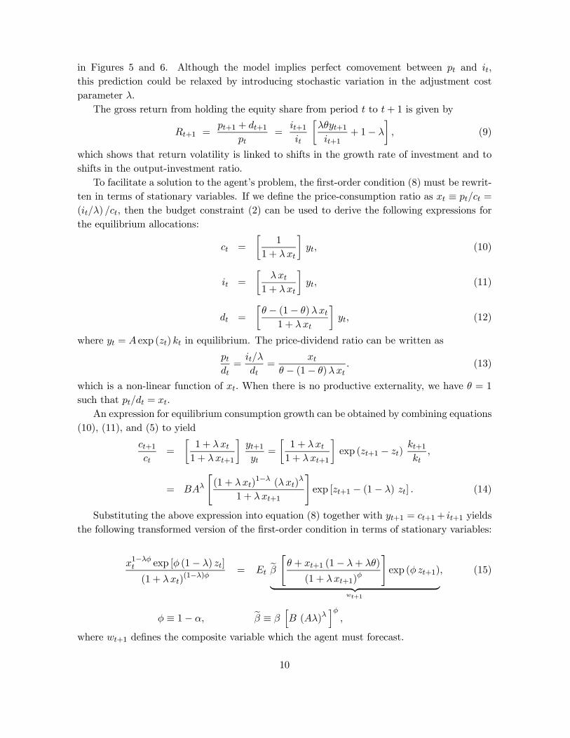
in Figures 5 and 6. Although the model implies perfect comovement between pt and it,

this prediction could be relaxed by introducing stochastic variation in the adjustment costparameter λ.

The gross return from holding the equity share from period t to t+ 1 is given by

Rt+1 =pt+1 + dt+1

pt=

it+1it

∙λθyt+1it+1

+ 1− λ

¸, (9)

which shows that return volatility is linked to shifts in the growth rate of investment and toshifts in the output-investment ratio.

To facilitate a solution to the agent’s problem, the first-order condition (8) must be rewrit-ten in terms of stationary variables. If we define the price-consumption ratio as xt ≡ pt/ct =

(it/λ) /ct, then the budget constraint (2) can be used to derive the following expressions forthe equilibrium allocations:

ct =

∙1

1 + λxt

¸yt, (10)

it =

∙λxt

1 + λxt

¸yt, (11)

dt =

∙θ − (1− θ)λxt

1 + λxt

¸yt, (12)

where yt = A exp (zt) kt in equilibrium. The price-dividend ratio can be written as

ptdt=

it/λ

dt=

xtθ − (1− θ)λxt

. (13)

which is a non-linear function of xt. When there is no productive externality, we have θ = 1such that pt/dt = xt.

An expression for equilibrium consumption growth can be obtained by combining equations(10), (11), and (5) to yield

ct+1ct

=

∙1 + λxt1 + λxt+1

¸yt+1yt

=

∙1 + λxt1 + λxt+1

¸exp (zt+1 − zt)

kt+1kt

,

= BAλ

"(1 + λxt)

1−λ (λxt)λ

1 + λxt+1

#exp [zt+1 − (1− λ) zt] . (14)

Substituting the above expression into equation (8) together with yt+1 = ct+1+ it+1 yieldsthe following transformed version of the first-order condition in terms of stationary variables:

x1−λφt exp [φ (1− λ) zt]

(1 + λxt)(1−λ)φ = Et

eβ "θ + xt+1 (1− λ+ λθ)

(1 + λxt+1)φ

#exp (φ zt+1)| {z }

wt+1

, (15)

φ ≡ 1− α, eβ ≡ βhB (Aλ)λ

iφ,

where wt+1 defines the composite variable which the agent must forecast.

10

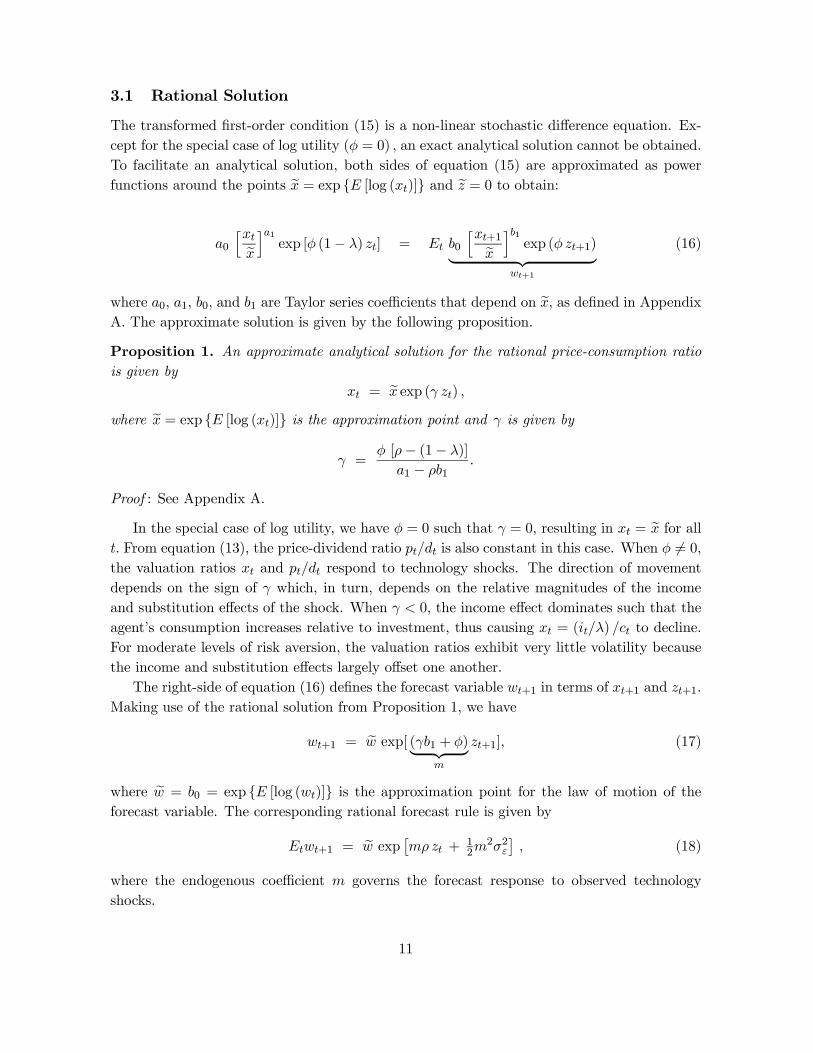
3.1 Rational Solution

The transformed first-order condition (15) is a non-linear stochastic difference equation. Ex-cept for the special case of log utility (φ = 0) , an exact analytical solution cannot be obtained.To facilitate an analytical solution, both sides of equation (15) are approximated as powerfunctions around the points ex = exp {E [log (xt)]} and ez = 0 to obtain:

a0

hxtex ia1 exp [φ (1− λ) zt] = Et b0

hxt+1ex ib1exp (φzt+1)| {z }

wt+1

(16)

where a0, a1, b0, and b1 are Taylor series coefficients that depend on ex, as defined in AppendixA. The approximate solution is given by the following proposition.

Proposition 1. An approximate analytical solution for the rational price-consumption ratiois given by

xt = ex exp (γ zt) ,where ex = exp {E [log (xt)]} is the approximation point and γ is given by

γ =φ [ρ− (1− λ)]

a1 − ρb1.

Proof : See Appendix A.

In the special case of log utility, we have φ = 0 such that γ = 0, resulting in xt = ex for allt. From equation (13), the price-dividend ratio pt/dt is also constant in this case. When φ 6= 0,the valuation ratios xt and pt/dt respond to technology shocks. The direction of movementdepends on the sign of γ which, in turn, depends on the relative magnitudes of the incomeand substitution effects of the shock. When γ < 0, the income effect dominates such that theagent’s consumption increases relative to investment, thus causing xt = (it/λ) /ct to decline.For moderate levels of risk aversion, the valuation ratios exhibit very little volatility becausethe income and substitution effects largely offset one another.

The right-side of equation (16) defines the forecast variable wt+1 in terms of xt+1 and zt+1.Making use of the rational solution from Proposition 1, we have

wt+1 = ew exp[ (γb1 + φ)| {z }m

zt+1], (17)

where ew = b0 = exp {E [log (wt)]} is the approximation point for the law of motion of theforecast variable. The corresponding rational forecast rule is given by

Etwt+1 = ew exp £mρzt +12m

2σ2ε¤, (18)

where the endogenous coefficient m governs the forecast response to observed technologyshocks.

11

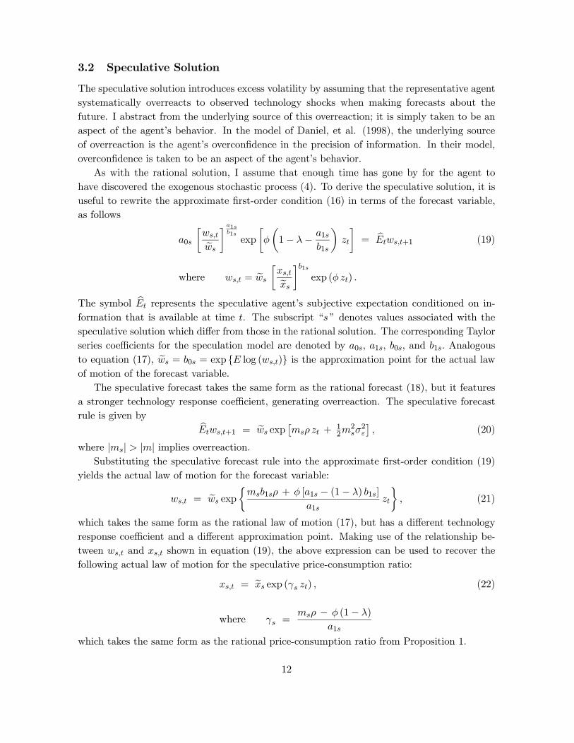
3.2 Speculative Solution

The speculative solution introduces excess volatility by assuming that the representative agentsystematically overreacts to observed technology shocks when making forecasts about thefuture. I abstract from the underlying source of this overreaction; it is simply taken to be anaspect of the agent’s behavior. In the model of Daniel, et al. (1998), the underlying sourceof overreaction is the agent’s overconfidence in the precision of information. In their model,overconfidence is taken to be an aspect of the agent’s behavior.

As with the rational solution, I assume that enough time has gone by for the agent tohave discovered the exogenous stochastic process (4). To derive the speculative solution, it isuseful to rewrite the approximate first-order condition (16) in terms of the forecast variable,as follows

a0s

∙ws,tews

¸a1sb1s

exp

∙φ

µ1− λ− a1s

b1s

¶zt

¸= bEtws,t+1 (19)

where ws,t = ews

∙xs,texs

¸b1sexp (φzt) .

The symbol bEt represents the speculative agent’s subjective expectation conditioned on in-formation that is available at time t. The subscript “s ” denotes values associated with thespeculative solution which differ from those in the rational solution. The corresponding Taylorseries coefficients for the speculation model are denoted by a0s, a1s, b0s, and b1s. Analogousto equation (17), ews = b0s = exp {E log (ws,t)} is the approximation point for the actual lawof motion of the forecast variable.

The speculative forecast takes the same form as the rational forecast (18), but it featuresa stronger technology response coefficient, generating overreaction. The speculative forecastrule is given by bEtws,t+1 = ews exp

£msρ zt +

12m

2sσ2ε

¤, (20)

where |ms| > |m| implies overreaction.Substituting the speculative forecast rule into the approximate first-order condition (19)

yields the actual law of motion for the forecast variable:

ws,t = ews exp

½msb1sρ + φ [a1s − (1− λ) b1s]

a1szt

¾, (21)

which takes the same form as the rational law of motion (17), but has a different technologyresponse coefficient and a different approximation point. Making use of the relationship be-tween ws,t and xs,t shown in equation (19), the above expression can be used to recover thefollowing actual law of motion for the speculative price-consumption ratio:

xs,t = exs exp (γs zt) , (22)

where γs =msρ − φ (1− λ)

a1s

which takes the same form as the rational price-consumption ratio from Proposition 1.

12

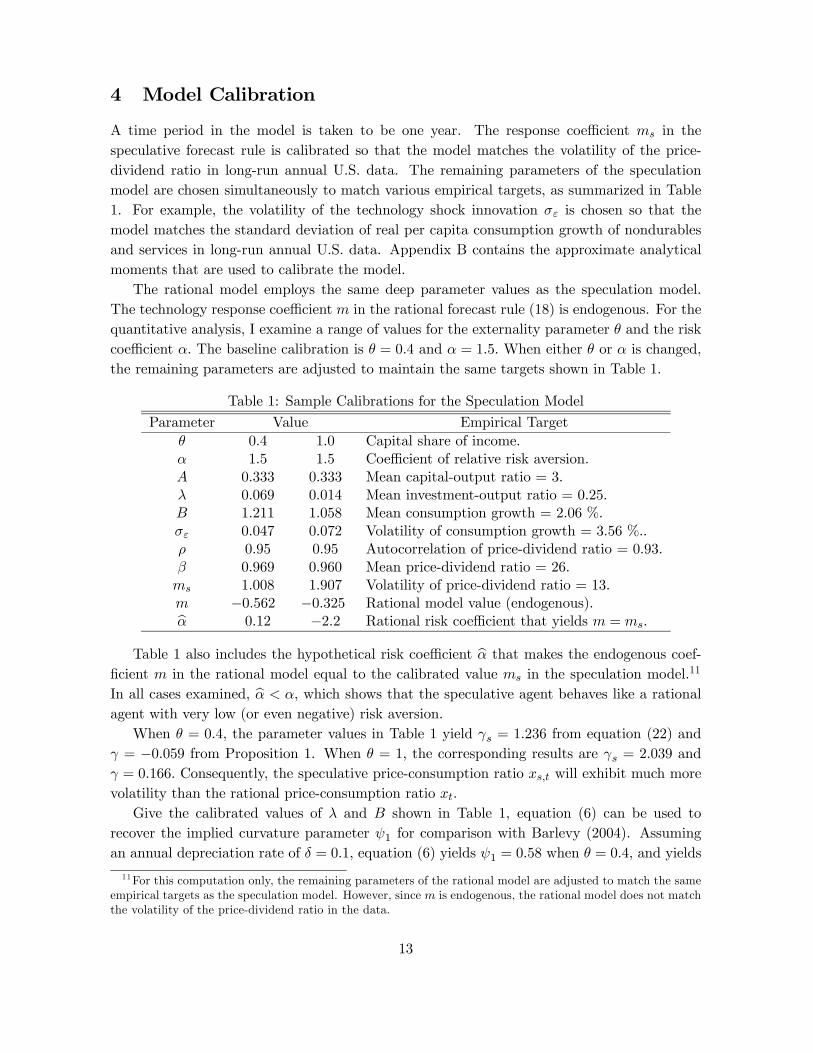
4 Model Calibration

A time period in the model is taken to be one year. The response coefficient ms in thespeculative forecast rule is calibrated so that the model matches the volatility of the price-dividend ratio in long-run annual U.S. data. The remaining parameters of the speculationmodel are chosen simultaneously to match various empirical targets, as summarized in Table1. For example, the volatility of the technology shock innovation σε is chosen so that themodel matches the standard deviation of real per capita consumption growth of nondurablesand services in long-run annual U.S. data. Appendix B contains the approximate analyticalmoments that are used to calibrate the model.

The rational model employs the same deep parameter values as the speculation model.The technology response coefficient m in the rational forecast rule (18) is endogenous. For thequantitative analysis, I examine a range of values for the externality parameter θ and the riskcoefficient α. The baseline calibration is θ = 0.4 and α = 1.5. When either θ or α is changed,the remaining parameters are adjusted to maintain the same targets shown in Table 1.

Table 1: Sample Calibrations for the Speculation Model

Parameter Value Empirical Targetθ 0.4 1.0 Capital share of income.α 1.5 1.5 Coefficient of relative risk aversion.A 0.333 0.333 Mean capital-output ratio = 3.λ 0.069 0.014 Mean investment-output ratio = 0.25.B 1.211 1.058 Mean consumption growth = 2.06 %.σε 0.047 0.072 Volatility of consumption growth = 3.56 %..ρ 0.95 0.95 Autocorrelation of price-dividend ratio = 0.93.β 0.969 0.960 Mean price-dividend ratio = 26.ms 1.008 1.907 Volatility of price-dividend ratio = 13.m −0.562 −0.325 Rational model value (endogenous).bα 0.12 −2.2 Rational risk coefficient that yields m = ms.

Table 1 also includes the hypothetical risk coefficient bα that makes the endogenous coef-ficient m in the rational model equal to the calibrated value ms in the speculation model.11

In all cases examined, bα < α, which shows that the speculative agent behaves like a rationalagent with very low (or even negative) risk aversion.

When θ = 0.4, the parameter values in Table 1 yield γs = 1.236 from equation (22) andγ = −0.059 from Proposition 1. When θ = 1, the corresponding results are γs = 2.039 andγ = 0.166. Consequently, the speculative price-consumption ratio xs,t will exhibit much morevolatility than the rational price-consumption ratio xt.

Give the calibrated values of λ and B shown in Table 1, equation (6) can be used torecover the implied curvature parameter ψ1 for comparison with Barlevy (2004). Assumingan annual depreciation rate of δ = 0.1, equation (6) yields ψ1 = 0.58 when θ = 0.4, and yields

11For this computation only, the remaining parameters of the rational model are adjusted to match the sameempirical targets as the speculation model. However, since m is endogenous, the rational model does not matchthe volatility of the price-dividend ratio in the data.

13

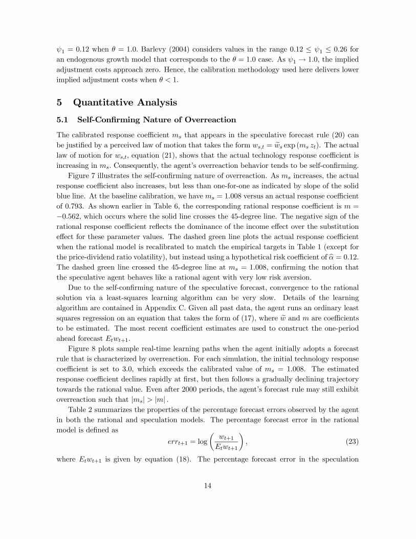
ψ1 = 0.12 when θ = 1.0. Barlevy (2004) considers values in the range 0.12 ≤ ψ1 ≤ 0.26 foran endogenous growth model that corresponds to the θ = 1.0 case. As ψ1 → 1.0, the impliedadjustment costs approach zero. Hence, the calibration methodology used here delivers lowerimplied adjustment costs when θ < 1.

5 Quantitative Analysis

5.1 Self-Confirming Nature of Overreaction

The calibrated response coefficient ms that appears in the speculative forecast rule (20) canbe justified by a perceived law of motion that takes the form ws,t = ews exp (ms zt). The actuallaw of motion for ws,t, equation (21), shows that the actual technology response coefficient isincreasing in ms. Consequently, the agent’s overreaction behavior tends to be self-confirming.

Figure 7 illustrates the self-confirming nature of overreaction. As ms increases, the actualresponse coefficient also increases, but less than one-for-one as indicated by slope of the solidblue line. At the baseline calibration, we have ms = 1.008 versus an actual response coefficientof 0.793. As shown earlier in Table 6, the corresponding rational response coefficient is m =

−0.562, which occurs where the solid line crosses the 45-degree line. The negative sign of therational response coefficient reflects the dominance of the income effect over the substitutioneffect for these parameter values. The dashed green line plots the actual response coefficientwhen the rational model is recalibrated to match the empirical targets in Table 1 (except forthe price-dividend ratio volatility), but instead using a hypothetical risk coefficient of bα = 0.12.The dashed green line crossed the 45-degree line at ms = 1.008, confirming the notion thatthe speculative agent behaves like a rational agent with very low risk aversion.

Due to the self-confirming nature of the speculative forecast, convergence to the rationalsolution via a least-squares learning algorithm can be very slow. Details of the learningalgorithm are contained in Appendix C. Given all past data, the agent runs an ordinary leastsquares regression on an equation that takes the form of (17), where ew and m are coefficientsto be estimated. The most recent coefficient estimates are used to construct the one-periodahead forecast Etwt+1.

Figure 8 plots sample real-time learning paths when the agent initially adopts a forecastrule that is characterized by overreaction. For each simulation, the initial technology responsecoefficient is set to 3.0, which exceeds the calibrated value of ms = 1.008. The estimatedresponse coefficient declines rapidly at first, but then follows a gradually declining trajectorytowards the rational value. Even after 2000 periods, the agent’s forecast rule may still exhibitoverreaction such that |ms| > |m| .

Table 2 summarizes the properties of the percentage forecast errors observed by the agentin both the rational and speculation models. The percentage forecast error in the rationalmodel is defined as

errt+1 = log

µwt+1

Etwt+1

¶, (23)

where Etwt+1 is given by equation (18). The percentage forecast error in the speculation

14

model is defined similarly, with bEtws,t+1 given by equation (20). The simulated time seriesfor wt and ws,t are computed by solving the original nonlinear first-order condition (15) ateach time step of the simulation, as described in Appendix C. Use of the approximate laws ofmotion (17) and (21) to generate the simulated time series produced similar results.

Table 2: Moments of Forecast Errors

θ = 0.4 θ = 1.0RationalModel

SpeculationModel

RationalModel

SpeculationModel

Mean 0.01 % 0.17 % 0.01 % −0.28 %RMSE 2.66 % 4.87 % 2.37 % 13.3 %Corr. Lag 1 −0.01 0.23 −0.01 0.01Corr. Lag 2 −0.01 0.21 −0.01 0.00Corr. Lag 3 −0.01 0.21 −0.01 0.01

Note: Statistics are from 10,000 period simulation with α = 1.5.

The table shows that forecast errors observed by the speculative agent are not persistent,particularly when θ = 1.0. Even when θ = 0.4, it would take a large amount of data for theagent to reject the null hypothesis of white noise forecast errors, especially given the samplingvariation in the autocorrelation statistics. Experiments with the model show that the forecasterrors become more persistent at higher levels of risk aversion. Intuitively, the vertical interceptof the solid blue line in Figure 8 becomes more negative as the risk coefficient α increases,thus producing a wider gap between the actual and perceived values of the technology responsecoefficient.

Although not shown in the table, one can also compute the forecast errors that arise whenthe fundamentals-based forecast rule (18) is used to predict the realized value of ws,t+1 in thespeculation model. These errors would be of interest to a speculative agent who is contem-plating a switch to a fundamentals-based forecast. In deciding whether to switch forecasts,the agent would keep track of the forecast errors associated with each method. Before anyswitch occurs, the actual law of motion for ws,t would still be governed by (21). In simulations,the fundamentals-based forecast significantly underperforms the speculative forecast rule (20)when predicting the realized value of ws,t+1. For example, when θ = 0.4, the RMSE of thefundamentals-based forecast is 19.6% versus only 4.87% for the speculative forecast. From theperspective of an individual agent, switching to a fundamentals-based forecast would appearto reduce forecast accuracy, so there is no incentive to switch. In other words, an individualagent can become “locked-in” to the speculative forecast if other agents are following the sameapproach.12

5.2 Model Simulations

This section examines the ability of the speculation model to match various features of U.S.data.12Lansing (2006) examines the concept of forecast lock-in using a standard Lucas-type asset pricing model.

15

Table 3 presents unconditional moments of asset pricing variables computed from a longsimulation of the model, where μdt+1 ≡ log (dt+1/dt) and μct+1 ≡ log (ct+1/ct) are the growthrates of dividends and consumption, respectively. The table also reports the correspondingstatistics from long-run U.S. data.13

Table 3: Unconditional Asset Pricing Moments

Statistic U.S. DataRationalModel

SpeculationModel

Mean pt/dt 25.9 23.9 26.7Std. Dev. 13.3 0.42 12.6Skew. 2.45 0.12 2.76Kurt. 9.82 3.00 17.5Corr. Lag 1 0.93 0.95 0.93Mean Rt 8.26 % 6.35 % 6.77 %Std. Dev. 17.7 % 4.84 % 9.29 %Corr. Lag 1 0.03 0.02 −0.03Mean μdt+1 1.20 % 1.96 % 1.92 %Std. Dev. 11.8 % 5.08 % 4.96 %Corr. Lag 1 0.12 0.01 0.10Mean μct+1 2.06 % 1.96 % 1.92 %Std. Dev. 3.56 % 4.80 % 3.59 %Corr. Lag 1 −0.08 0.01 0.27Note: Model statistics are from 10,000 period simulation with θ = 0.4, α = 1.5.

Recall that the speculation model is calibrated to match the mean, volatility, and persis-tence of the price-dividend ratio in the data. But the model also does a good job of matchingthe higher moments; the U.S. ratio exhibits positive skewness and excess kurtosis, which sug-gest the presence of nonlinearities in the data which the model is able to capture. In contrast,the rational solution delivers very low volatility, near-zero skewness, and no excess kurtosis.The persistence of the rational price-dividend ratio does match the data, however, since it isinherited directly from the technology shock process with ρ = 0.95.

The mean equity return for both models is a bit below the long-run U.S. average of 8.26%.The volatility of returns in the speculation model is about twice that of the rational model, butstill significantly below the return volatility of 17.7% in the data. The reason the speculationmodel undepredicts the return volatility is because it undepredicts the volatility of dividendgrowth, which is one component of the return. The volatility of dividend growth in both modelsis around 5% whereas the corresponding figure in the data is nearly 12%. From equation (12),the volatility of dividend growth in either model could be increased by introducing stochasticvariation in the production function parameter θ.

The speculation model is calibrated to match the first and second moments of consumptiongrowth in the data, but nevertheless there is a small difference between the model mean of13The sample periods for the U.S. data are as follows: price-dividend ratio 1871-2004, real equity return 1871-

2004, real consumption growth 1890-2004, real dividend growth 1872-2004. The price-dividend ratio in year tis defined as the value of the S&P 500 stock index at the beginning of year t+ 1, divided by the accumulateddividend over year t.

16

1.92% and the data mean of 2.06%. This result is due to the approximate moment formulaused in the calibration (see Appendix B), whereas the simulations make use of the non-linearequilibrium conditions. Consumption growth in the speculation model exhibits some positiveserial correlation, with a coefficient of 0.27, whereas the serial correlation in the long-run datais slightly negative at −0.08. Azerado (2007) argues that better measures of food and servicesconsumption in the sample period prior to 1930 yields a positive serial correlation coeffcientof 0.32 for the long-run data, which is close to the speculation model’s prediction.

Figure 9 plots simulations from both models for the baseline calibration with θ = 0.4 andα = 1.5. In the top left panel, the highly persistent and volatile nature of the speculative price-dividend ratio gives rise to intermittent excursions away from the rational (or fundamental)value. Interestingly, the speculation model can also generate prolonged periods where the price-dividend ratio remains in close proximity to the rational value. At the baseline calibration,we have γs = 1.236, which implies that the speculative valuation ratios increase in responseto a positive technology shock. The technology-driven bubble episodes in the model coincidewith economic booms and excess capital formation, as shown in the lower panels of Figure 9.These episodes are reminiscent of the U.S. economy during the late 1920s and late 1990s.

Figure 10 plots the cyclical components of the macroeconomic variables from the modelsimulations.14 Table 4 compares the relative volatilities of the detrended series. In the rationalmodel, the presence of capital adjustment costs makes the volatility of investment about thesame as the volatility of consumption, which is counterfactual. In U.S. data, investment isabout three times more volatile than consumption. By construction, the speculation modelmagnifies asset price volatility which is linked directly to investment volatility. Given thatoutput volatility in the two models is about the same, the excess volatility of investment inthe speculation model reduces the resulting consumption volatility relative to the rationalbenchmark. This result has important implications for the welfare analysis, which is discussedin the next section.

Table 4: Volatility of Detrended Macroeconomic Variables

VariableRationalModel

SpeculationModel

yt 3.08 3.00ct 3.13 2.04it 2.94 5.94dt 3.32 3.18

Note: In percent. From 2000 period simulation with θ = 0.4, α = 1.5.

5.3 Welfare Cost of Speculation and Business Cycles

This section examines the welfare costs of fluctuations that can be attributed to either: (i)speculative behavior, or (ii) business cycles. Welfare costs are measured by the percentage

14The cyclical components are obtained by detrending each series with the Hodrick-Prescott filter using asmoothing parameter of 10, as recommended by Baxter and King (1999) for annual data.

17

change in per-period consumption that makes the agent indifferent between the two economiesbeing compared. The details of the welfare computations are contained in Appendix D.

The basic intuition underlying the welfare results is as follows:

• Fluctuations that are driven by speculation or business cycles can affect both the meanand volatility of consumption growth.

• A decrease in mean consumption growth is associated with a smaller fraction of resourcesdevoted to investment, and hence a higher initial level of consumption. Higher initialconsumption can mitigate the welfare costs of slower growth.

• Higher initial consumption is less desirable from a welfare standpoint when agents un-derinvest, i.e., when θ < 1.

• As risk aversion increases, consumption growth volatility becomes more costly in termsof welfare.

Which of these various effects dominate depends crucially on parameter values. Table 5summarizes the moments of log (ct+1/ct) for three different versions of the model. For eachvalue of the risk coefficient α, the speculation model is calibrated to match the mean andvolatility of consumption growth in long-run U.S. data.15

Fluctuations in the price-consumption ratio affect the mean and volatility of consumptiongrowth via equation (14), which is nonlinear. Depending on the degree of risk aversion, specu-lation may increase or decrease mean consumption growth relative to the rational benchmark.Table 5 shows that when risk aversion is very low, speculation increases mean consumptiongrowth relative to the rational benchmark, while the reverse holds true for higher risk aversion.But for any degree of risk aversion, speculation reduces the volatility of consumption growthrelative to the rational benchmark, consistent with the earlier discussion of Figure 10 andTable 4.

Further insight into the effect of fluctuations on investment and growth can be obtainedfrom the investment allocation rule (11). The rule implies

∂ (it/yt)

∂xt=

λ

(1 + λxt)2 > 0, (24)

which shows that it/yt is an increasing concave function of the price-consumption ratio xt. Asshown in Appendix A, the approximation point for the (rational) price-consumption ratio isgiven by the following expression

ex = exp {E [log (xt)]} = θβ exp£φeμ+m2σ2/2

¤1− β (1− λ+ λθ) exp [φeμ+m2σ2/2]

, (25)

15The small differences in Table 5 between the consumption growth moments of the speculation model andthose in U.S. data can be traced to the approximate moment formulas used in the model calibration, whereasthe model simulations make use of the actual non-linear equilibrium conditions.

18

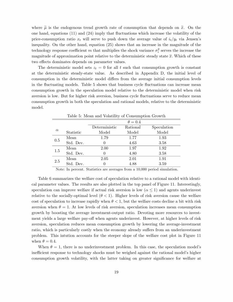
where eμ is the endogenous trend growth rate of consumption that depends on ex. On theone hand, equations (11) and (24) imply that fluctuations which increase the volatility of theprice-consumption ratio xt will serve to push down the average value of it/yt via Jensen’sinequality. On the other hand, equation (25) shows that an increase in the magnitude of thetechnology response coefficient m that multiplies the shock variance σ2 serves the increase themagnitude of approximation point relative to the deterministic steady state x.Which of thesetwo effects dominates depends on parameter values.

The deterministic model sets zt = 0 for all t such that consumption growth is constantat the deterministic steady-state value. As described in Appendix D, the initial level ofconsumption in the deterministic model differs from the average initial consumption levelsin the fluctuating models. Table 5 shows that business cycle fluctuations can increase meanconsumption growth in the speculation model relative to the deterministic model when riskaversion is low. But for higher risk aversion, business cycle fluctuations serve to reduce meanconsumption growth in both the speculation and rational models, relative to the deterministicmodel.

Table 5: Mean and Volatility of Consumption Growth

θ = 0.4

αStatistic

DeterministicModel

RationalModel

SpeculationModel

0.5MeanStd. Dev.

1.790

1.774.63

1.933.58

1.5MeanStd. Dev.

2.000

1.974.80

1.923.58

2.5MeanStd. Dev.

2.050

2.014.88

1.913.59

Note: In percent. Statistics are averages from a 10,000 period simulation.

Table 6 summarizes the welfare cost of speculation relative to a rational model with identi-cal parameter values. The results are also plotted in the top panel of Figure 11. Interestingly,speculation can improve welfare if actual risk aversion is low (α ≤ 1) and agents underinvestrelative to the socially-optimal level (θ < 1). Higher levels of risk aversion cause the welfarecost of speculation to increase rapidly when θ < 1, but the welfare costs decline a bit with riskaversion when θ = 1. At low levels of risk aversion, speculation increases mean consumptiongrowth by boosting the average investment-output ratio. Devoting more resources to invest-ment yields a large welfare pay-off when agents underinvest. However, at higher levels of riskaversion, speculation reduces mean consumption growth by lowering the average-investmentratio, which is particularly costly when the economy already suffers from an underinvestmentproblem. This intution accounts for the steeper slope of the welfare cost plot in Figure 11when θ = 0.4.

When θ = 1, there is no underinvestment problem. In this case, the speculation model’sinefficient response to technology shocks must be weighed against the rational model’s higherconsumption growth volatility, with the latter taking on greater significance for welfare at

19

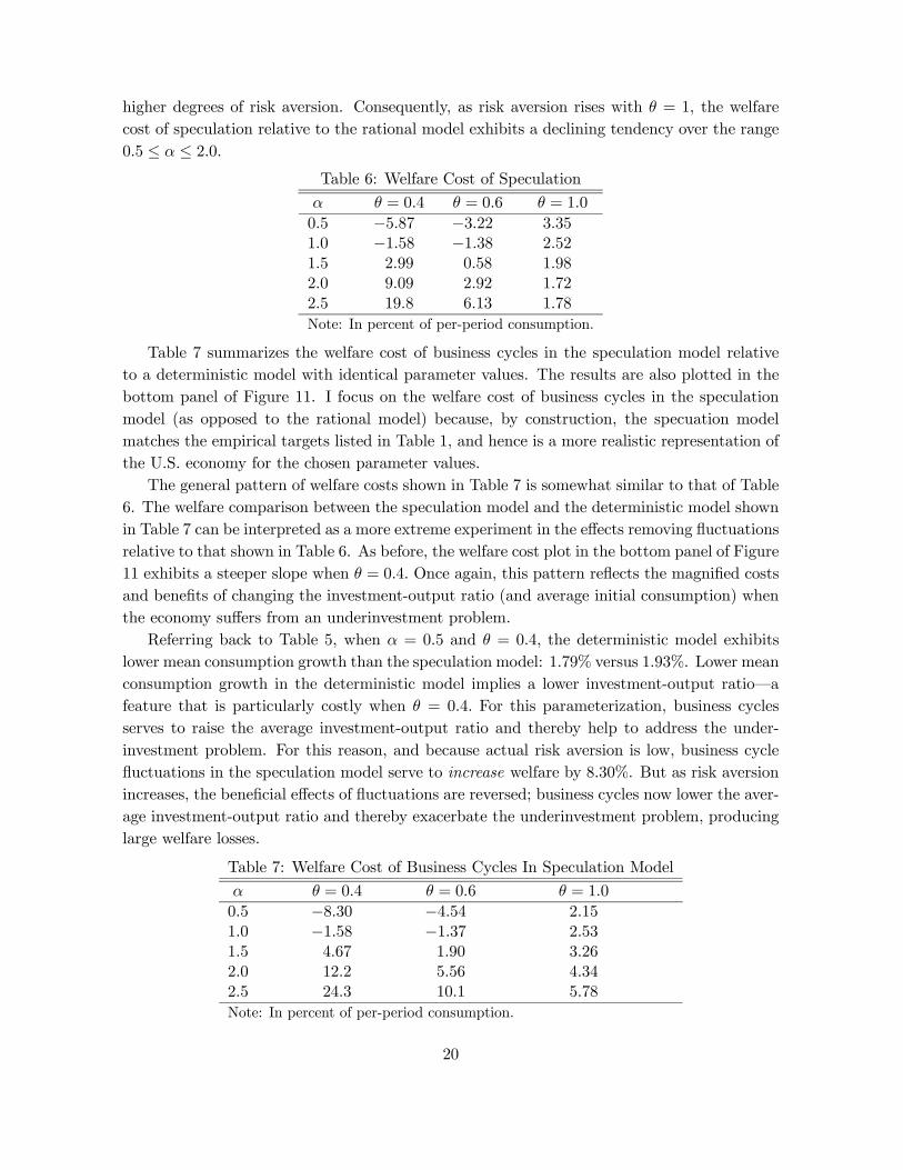
higher degrees of risk aversion. Consequently, as risk aversion rises with θ = 1, the welfarecost of speculation relative to the rational model exhibits a declining tendency over the range0.5 ≤ α ≤ 2.0.

Table 6: Welfare Cost of Speculation

α θ = 0.4 θ = 0.6 θ = 1.0

0.5 −5.87 −3.22 3.351.0 −1.58 −1.38 2.521.5 2.99 0.58 1.982.0 9.09 2.92 1.722.5 19.8 6.13 1.78

Note: In percent of per-period consumption.

Table 7 summarizes the welfare cost of business cycles in the speculation model relativeto a deterministic model with identical parameter values. The results are also plotted in thebottom panel of Figure 11. I focus on the welfare cost of business cycles in the speculationmodel (as opposed to the rational model) because, by construction, the specuation modelmatches the empirical targets listed in Table 1, and hence is a more realistic representation ofthe U.S. economy for the chosen parameter values.

The general pattern of welfare costs shown in Table 7 is somewhat similar to that of Table6. The welfare comparison between the speculation model and the deterministic model shownin Table 7 can be interpreted as a more extreme experiment in the effects removing fluctuationsrelative to that shown in Table 6. As before, the welfare cost plot in the bottom panel of Figure11 exhibits a steeper slope when θ = 0.4. Once again, this pattern reflects the magnified costsand benefits of changing the investment-output ratio (and average initial consumption) whenthe economy suffers from an underinvestment problem.

Referring back to Table 5, when α = 0.5 and θ = 0.4, the deterministic model exhibitslower mean consumption growth than the speculation model: 1.79% versus 1.93%. Lower meanconsumption growth in the deterministic model implies a lower investment-output ratio–afeature that is particularly costly when θ = 0.4. For this parameterization, business cyclesserves to raise the average investment-output ratio and thereby help to address the under-investment problem. For this reason, and because actual risk aversion is low, business cyclefluctuations in the speculation model serve to increase welfare by 8.30%. But as risk aversionincreases, the beneficial effects of fluctuations are reversed; business cycles now lower the aver-age investment-output ratio and thereby exacerbate the underinvestment problem, producinglarge welfare losses.

Table 7: Welfare Cost of Business Cycles In Speculation Model

α θ = 0.4 θ = 0.6 θ = 1.0

0.5 −8.30 −4.54 2.151.0 −1.58 −1.37 2.531.5 4.67 1.90 3.262.0 12.2 5.56 4.342.5 24.3 10.1 5.78

Note: In percent of per-period consumption.

20

Overall, the main message from Tables 6 and 7 is that speculation and business cyclescan be very costly as risk aversion increases. For the baseline parametrization with a riskcoefficient of α = 1.5, the welfare costs in Tables 6 and 7 range from a low of 0.58% to a high4.67%.

Barlevy (2004) estimates that eliminating business cycles can yield welfare gains of around7 percent of per-period consumption when holding initial consumption fixed in an endogenousgrowth model with logarithmic utility (α = 1) and no productive externality (θ = 1) . Barlevy’srational model is calibrated to match post-World War II data, whereas the speculation modelconsidered here is calibrated to match long-run data prior to the year 1900. Interestingly,the welfare costs of business cycles in the speculation model with θ = 1 are not too farfrom Barlevy’s results, despite differences in the capital adjustment cost formulation and thecalibration methodology. Qualitatively, the results presented in Table 7 are consistent withBarlevy’s finding that the welfare cost of business cycles can be large when long-run growthis endogenous.

6 Concluding Remarks

“Nowhere does history indulge in repetitions so often or so uniformly as in Wall Street,”observed legendary speculator Jesse Livermore.16 History tells us that periods of major tech-nological innovation are typically accompanied by speculative bubbles as agents overreact togenuine advancements in productivity. Excessive run-ups in asset prices can have importantconsequences for the economy because mispriced assets imply some form of capital misalloca-tion. Innovations to technology are also considered by many economists to be an importantdriving force for business cycles.

This paper developed a behavioral real business cycle model in which speculative agentsoverreact to observed technology shocks. Overreaction tends to be self-confirming; the forecasterrors observed by the speculative agent are not persistent for moderate levels of risk aversion.The speculation model outperformed the rational model in capturing several features of long-run U.S. data, including the higher moments of asset pricing variables and the relative volatilityof detrended consumption and investment.

Interestingly, even from the narrow perspective of the theoretical model, it remains anopen question whether the costs of speculative behavior outweigh the possible benefits tosociety. Speculation can affect the mean and volatility of consumption growth, as well as theagent’s average initial consumption level. Which of these various effects dominate in termsof welfare depends crucially on the degree of risk aversion and the severity of the economy’sunderinvestment problem.

It should be noted, of course, that the model abstracts from numerous real-world issuesthat would affect investors’ welfare. One noteworthy example is financial fraud. Throughouthistory, speculative bubbles have usually coincided with outbreaks of fraud and scandal, fol-lowed by calls for more government regulation once the bubble has burst. Indeed, the term

16From Livermore’s thinly-disguised biography by E. Lefevére (1923, p. 180).

21

“bubble” was coined in England in 1720 following the famous price run-up and crash of sharesin the South Sea Company. The run-up led to widespread public enthusiasm for the stock mar-ket and an explosion of highly suspect companies attempting to sell shares to investors. Onesuch venture notoriously advertised itself as “a company for carrying out an undertaking ofgreat advantage, but nobody to know what it is.” The proliferation of fraudulent stock-offeringschemes led the British government to pass the so-called “Bubble Act” in 1720.17

The idea that speculation may yield benefits to society has a long history. Regarding themerits of speculation, J. Edward Meeker (1922, p. 419), the economist of the New York StockExchange, wrote:

“Of all the peoples in history, the American people can least afford to condemnspeculation...The discovery of America was made possible by a loan based on thecollateral of Queen Isabella’s crown jewels, and at interest, beside which even thecall rates of 1919-1920 look coy and bashful. Financing an unknown foreignerto sail the unknown deep in three cockleshell boats in the hope of discovering amythical Zipangu [land of gold] cannot, by the wildest exercise of language, becalled a ‘conservative investment.’ ”

17The law was officially named “An Act to Restrain the Extravagant and Unwarrantable Practice of RaisingMoney by Voluntary Subscription for Carrying on Projects Dangerous to the Trade and Subjects of the UnitedKingdom.” See Gerding (2006).

22

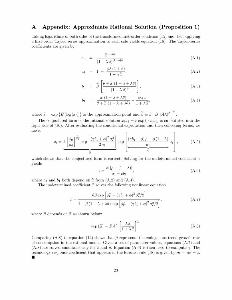
A Appendix: Approximate Rational Solution (Proposition 1)

Taking logarithms of both sides of the transformed first-order condition (15) and then applyinga first-order Taylor series approximation to each side yields equation (16). The Taylor-seriescoefficients are given by

a0 =ex1−λφ

(1 + λ ex)(1−λ)φ , (A.1)

a1 = 1 − φλ (1 + ex)1 + λ ex , (A.2)

b0 = eβ "θ + ex (1− λ+ λθ)

(1 + λ ex)φ#, (A.3)

b1 =ex (1− λ+ λθ)

θ + ex (1− λ+ λθ)− φλ ex1 + λ ex, (A.4)

where ex = exp {E [log (xt)]} is the approximation point and eβ ≡ βhB (Aλ)λ

iφ.

The conjectured form of the rational solution xt+1 = ex exp (γ zt+1) is substituted into theright-side of (16). After evaluating the conditional expectation and then collecting terms, wehave:

xt = ex ∙ b0a0

¸ 1a1

exp

"(γb1 + φ)2 σ2

2 a1

#| {z }

x

exp

⎡⎢⎢⎣(γb1 + φ) ρ− φ (1− λ)

a1| {z }γ

zt

⎤⎥⎥⎦ , (A.5)

which shows that the conjectured form is correct. Solving for the undetermined coefficient γyields

γ =φ [ρ− (1− λ)]

a1 − ρb1, (A.6)

where a1 and b1 both depend on ex from (A.2) and (A.4).The undetermined coefficient ex solves the following nonlinear equation

ex = θβ exphφeμ+ (γb1 + φ)2 σ2/2

i1− β (1− λ+ λθ) exp

hφeμ+ (γb1 + φ)2 σ2/2

i , (A.7)

where eμ depends on ex as shown below:exp (eμ) = BAλ

∙λ ex

1 + λ ex¸λ

. (A.8)

Comparing (A.8) to equation (14) shows that eμ represents the endogenous trend growth rateof consumption in the rational model. Given a set of parameter values, equations (A.7) and(A.8) are solved simultaneously for ex and eμ. Equation (A.6) is then used to compute γ. Thetechnology response coefficient that appears in the forecast rule (18) is given by m = γb1+φ.¥

23

B Appendix: Approximate Moments for Calibration

The Taylor series coefficients for the speculation model are denoted by a0s, a1s, b0s, and b1s.These coefficients take the same form as equations (A.1) through (A.4), but ex is now replacedby exs. Analogous to the rational solution, we have ews = b0s = exp {E [log (ws,t)]} .

The approximation point exs = exp {E [log (xs,t)]} is the solution to the following nonlinearequation exs = θβ exp

£φeμs +m2

sσ2/2¤

1− β (1− λ+ λθ) exp [φeμs +m2sσ2/2]

, (B.1)

where eμs depends on exs, as shown below:exp (eμs) = BAλ

∙λ exs

1 + λ exs¸λ

. (B.2)

Comparing (B.2) to equation (14) shows that eμs represents the endogenous trend growth rateof consumption in the speculation model. Given a set of parameter values and the exogenoustechnology response coefficient ms, equations (B.1) and (B.2) are solved simultaneously for exsand eμs. The response coefficient that appears in the approximate law of motion (22) for xs,tis then given by γs = [msρ − φ (1− λ)] /a1s.

Starting from equation (13), a Taylor series approximation for the speculative price-dividend ratio is given by

ps,tds,t

=

∙ exsθ − (1− θ)λ exs

¸ ∙xs,texs

¸ns, (B.3)

where ns = 1 +

∙(1− θ)λ exs

θ − (1− θ)λ exs¸.

The above expression implies the following unconditional moments:

E [log (ps,t/ds,t)] = log

∙ exsθ − (1− θ)λ exs

¸, (B.4)

V ar [log (ps,t/ds,t)] = n2s V ar [log (xs,t)] ,

= n2sγ2s V ar (zt) , (B.5)

Corr [log (ps,t/ds,t) , log (ps,t−1/ds,t−1)] = Corr [log (xs,t) , log (xs,t−1)] ,= Corr [zt, zt−1] ,= ρ. (B.6)

Given equations (B.4) and (B.5), the unconditional mean and variance of ps,t/ds,t can becomputed by making use of the properties of the log-normal distribution.18

18 If a random variable vt is log-normally distributed, then E (vt) = exp E [log (vt)] +12V ar [log (vt)] and

V ar (vt) = E (vt)2 {exp (V ar [log (vt)])− 1} .

24

Starting from (14), a Taylor series approximation for consumption growth in the specula-tion model is given by

cs,t+1cs,t

= exp (eμs) ∙xs,texs¸a2s ∙xs,t+1exs

¸b2sexp [zt+1 − (1− λ) zt] , (B.7)

where a2s =λ (1 + exs)1 + λ exs , b2s =

−λ exs1 + λ exs ,

and exp (eμs) is given by equation (B.2). Given the approximate law of motion (22) for xs,t,the above expression implies the following unconditional moments

E [log (cs,t+1/cs,t)] = eμs, (B.8)

V ar [log (cs,t+1/cs,t)] =n(γsa2s − 1 + λ)2 + (γsb2s + 1)

2

+ 2ρ (γsa2s − 1 + λ) (γsb2s + 1)} V ar (zt) . (B.9)

C Appendix: Learning and Nonlinear Model Simulations

Real-time learning is discussed in Section 5.1 of the text. The learning algorithm is describedby the following system of nonlinear stochastic difference equations:

x1−λφt exp [(1− λ)φ zt]

(1 + λxt)(1−λ)φ = ewt−1 exp

£mt−1 ρ zt + 1

2m2t−1σ

2ε

¤| {z }Etwt+1

, (C.1)

wt ≡ eβ "θ + xt (1− λ+ λθ)

(1 + λxt)φ

#exp (φzt) , (C.2)

log (wt) = log ( ewt) +mt zt, (C.3)

where zt is governed by equation (4). Equation (C.1) is the nonlinear first-order conditionwhere the right side defines the agent’s conditional forecast using the most recent forecastrule coefficients ewt−1 and mt−1. Given the conditional forecast and the current observed valueof zt, the left side of (C.1) is solved for xt using a nonlinear equation solver. Given xt andzt, the nonlinear definitional relationship (C.2) is used to compute the current realization ofthe composite variable wt. Given all past data on wt and zt, the agent runs an ordinary leastsquares regression in the form of (C.3) to obtain a new set of forecast rule coefficients ewt andmt.

The model simulations described in Section 5.1 and 5.2 employ an algorithm that is similarto (C.1) and (C.2), except that the forecast rule coefficients are held constant throughout thesimulation. The rational forecast rule coefficients are ew = b0 and m. The speculative forecastrule coefficients are ews = b0s and ms.

For both the learning algorithm and the model simulations, the initial condition for theprice-consumption ratio and the forecast variable is the deterministic steady state. The spec-ulation model and the rational model have the same steady state. The steady-state price-consumption ratio is denoted by x. Steady-state consumption growth is denoted by μ. The

25

values of x and μ solve the following system of nonlinear equations

x =θβ exp (φμ)

1− β (1− λ+ λθ) exp (φμ), (C.4)

exp (μ) = BAλ

∙λx

1 + λx

¸λ. (C.5)

Given x, the steady-state value of the forecast variable is computed from:

w = βhB (Aλ)λ

iφ "θ + x (1− λ+ λθ)

(1 + λx)φ

#. (C.6)

D Appendix: Details of Welfare Cost Computation

This appendix describes the procedure for computing the welfare costs presented in Tables 6and 7.

D.1 Welfare Cost of Speculation

Average lifetime utility in the rational model is represented by V. Average lifetime utility inthe speculation model is represented Vs. These welfare measures can be written as

V =−1

φ (1− β)+E

∞Xt=0

βt(ct)

φ

φ, φ ≡ 1− α, (D.1)

Vs =−1

φ (1− β)+E

∞Xt=0

βt(cs,t)

φ

φ, (D.2)

where ct = yt/ (1 + λxt) and cs,t = ys,t/ (1 + λxs,t) are the nonlinear allocation rules thatgovern the consumption streams. During a simulation, xt and xs,t are computed using thenonlinear algorithm described in Appendix C. The unconditional mean E is approximatedby the average over 5000 simulations, each 2000 periods in length, after which the resultsare little changed. The initial consumption levels at t = 0 are stochastic variables. Eachsimulation starts at t = −1 with yt = ys,t = 1, such that ct = cs,t = 1/ (1 + λx) , where x isthe steady-state price-consumption ratio from equation (C.4).

The welfare cost of speculation is the constant percentage amount by which cs,t must beincreased in the speculation model in order to make average lifetime utility equal to that inthe rational model. Specifically, I solve for τ such that

V =−1

φ (1− β)+E

∞Xt=0

βt[cs,t (1 + τ)]φ

φ.

=−1

φ (1− β)+ (1 + τ)φ

∙Vs +

1

φ (1− β)

¸, (D.3)

which yields the result

τ =

∙φ (1− β)V + 1

φ (1− β)Vs + 1

¸ 1φ

− 1. (D.4)

In the case of log utility (φ = 0) , equation (D.4) becomes τ = exp [(V − Vs) (1− β)]− 1.

26

D.2 Welfare Cost of Business Cycles

The welfare cost of business cycles in the calibrated speculation model is the constant percent-age amount by which cs,t must be increased in order to make average lifetime utility equal tothat of a deterministic model with zt = 0 for all t. Lifetime utility in the deterministic modelVd can be written as

Vd =−1

φ (1− β)+

∞Xt=0

βt(cd,t)

φ

φ. (D.5)

The deterministic simulation starts at t = −1 with yd,t = 1, such that cd,t = 1/ (1 + λx) ,where x is given by equation (C.4). Deterministic consumption evolves according to the law ofmotion cd,t = cd,t−1 exp (μ) , where μ is given by equation (C.5). Deterministic consumptionat t = 0 will thus differ from average consumption at t = 0 in the fluctuating model.

Analogous to equation (D.4), the welfare cost of business cycles in the speculation modelis given by

τ =

∙φ (1− β)Vd + 1

φ (1− β)Vs + 1

¸ 1φ

− 1. (D.6)

In the case of log utility, (φ = 0) , equation (D.6) becomes τ = exp [(Vd − Vs) (1− β)]− 1.

27

References

Abel, A.B. (2002) “An exploration of the effects of pessimism and doubt on asset returns,”Journal of Economic Dynamics and Control 26, 1075-1092.

Adam, K., A. Marcet, and J.P. Nicolini 2008 Stock market volatility and learning, Workingpaper.

Abreu, D. and M.K. Brunnermeier (2003) “Bubbles and crashes,” Econometrica 71, 173-204.

Arbarbanell, J.S. and V.L. Bernard (1992) “Tests of analysts’ over-reaction/under-reactionto earnings information as an explanation for anomalous stock price behavior,” Journal ofFinance 47, 1181-1207.

Angeletos, G.-M., G. Lorenzoni, and A. Pavan (2007) “Wall Street and Silicon Valley: Adelicate interaction,” National Bureau of Economic Research, Working Paper 13475.

Arrow, K.J. (1962). “The Economic Implications of Learning by Doing,” Review of EconomicStudies 29, 155-173.

Azerado, F. (2007). “The equity premium: A deeper puzzle,” Working Paper, University ofCalifornia, Santa Barbara.

Barberis, N., A. Shleifer, and R.W. Vishny (1998) “A model of investor sentiment,” Journalof Financial Economics 49, 307-343.

Barlevy, G. (2004), “The cost of business cycles under endogenous growth,” American Eco-nomic Review 94, 964-990.

Barlevy, G. (2007), “Economic theory and asset bubbles,” Federal Reserve Bank of Chicago,Economic Pespectives 3Q, 44-59.

Barro, R.J. (1990), “The stock market and investment,” Review of Financial Studies, 3, 115-131.

Barsky, R.B. and J.B. De Long (1993) “Why does the stock market fluctuate?” QuarterlyJournal of Economics 107, 291-311.

Baxter, M. and R.G. King. (1999). “Measuring business cycles: Approximate band-pass filtersfor economic time series,” Review of Economics and Statistics 81, 575-593.

Borio, C. and P. Lowe (2002) “Asset prices, financial and monetary stability: Exploring thenexus.” Bank of International Settlements, Working Paper 114.

Caballero, R. J. E. Farhi, and M.L. Hammour (2006) “Speculative growth: Hints from theU.S. economy,” American Economic Review, 96, 1159-1192.

Campello, M. and J. Graham (2007) “Do stock prices influence corporate decisions? Evidencefrom the technology bubble,” National Bureau of Economic Research, Working Paper 13640.

Cecchetti, S.G., P.-S. Lam, and N.C. Mark (2000) “Asset pricing with distorted beliefs: Areequity returns too good to be true?” American Economic Review 90, 787-805.

Chirinko, R.S. and H. Schaller (2001) “Business fixed investment and ‘bubbles’: The Japanesecase,” American Economic Review 91, 663-680.

Chirinko, R.S. and H. Schaller (2007) “Fundamentals, misvaluation, and investment: The realstory,” Working Paper.

Christiano, L., C. Ilut, R. Motto, and M. Rostagno (2007) “Monetary policy and stock marketboom-bust cycles,” Working Paper.

28

Cooper, M.J., O. Dimitrov, and P. R. Rau (2001) “A Rose.com by any other name,” Journalof Finance, 54, 2371-2388.

Daniel, K., D. Hirshleifer D. and A. Subrahmanyam (1998) “Investor psychology, and securitymarket under- and overreactions, Journal of Finance 53, 1839-1186Debondt, W.F.M. and R. Thaler (1985) “Does the stock market overeact?” Journal of Finance40, 793-805.

Delong, J.B., A. Shleifer, L.H. Summers, and R.J. Waldmann (1990) “Noise trader risk infinancial markets,” Journal of Political Economy 98, 703-738.

Dupor, B. (2002) “The natural rate of Q,”American Economic Review, Papers and Proceedings92, 96-101.

Dupor, B. (2005) “Stabilizing non-fundamental asset price movements under discretion andlimited information,” Journal of Monetary Economics 52 727-747.

Easterwood, J.C. and S.R. Nutt (1999) “Inefficiency in analysts’ earnings forecasts: systematicmisreaction or systematic optimism?” Journal of Finance 54, 1777-1797.

Feldstein, M.S. (2007) “Housing, credit markets, and the business cycle,” NBER WorkingPaper 13471.

Gerding, E.F. (2006) “The next epidemic: Bubbles and the growth and decay of securitiesregulation,” Connecticut Law Review, 38(3), 393-453.

Gilchrist, S., C. P. Himmelberg, and G. Huberman (2005) “Do stock price bubbles influencecorporate investment?” Journal of Monetary Economics 52 805-827.

Gordon, R.J. (2000) “Does the ‘New Economy’ Measure Up to the Great Inventions of thePast?” Journal of Economic Perspectives 14, 49-74.

Gordon, R.J. (2003) “Hi-Tech Innovation and Productivity Growth: Does Supply Create ItsOwn Demand?” NBER Working Paper 9437.

Gordon, R.J. (2006) “The 1920s and the 1990s in mutual reflection,” in The Global Economyin the 1990s, P.W. Rhode and G. Toniolo, eds., Cambridge University Press, pp. 161-192.

Greenspan, A. (2000) “Technology and the economy,” Remarks before the Economic Club ofNew York, New York City, January 13.

Greenspan, A. (2002) “Economic volatility,” Remarks at a symposium sponsored by the Fed-eral Reserve Bank of Kansas City, Jackson Hole, Wyoming, August 30.

Greenspan, A. (2005) “Consumer Finance,” Remarks at the Federal Reserve System’s FourthAnnual Community Affairs Research Conference, Washington, D.C., April 8.

Greenwood, J. and B. Jovanovic (1999) The information-technology revolution and the stockmarket,” American Economic Review, Papers and Proceedings 89, 116-122.

Grossman, G.M. and N. Yanagawa (1993) “Asset bubbles and endogenous growth,” Journalof Monetary Economics 31, 3-19.

Hall. R.E. (2001) “The stock market and capital accumulation,” American Economic Review91, 1185-1202.

Harrison, J.M. and D.K. Kreps (1978) “Speculative investor behavior in a stock market withheterogenous expectations,” Quarterly Journal of Economics, 92 323-336.

Hassan, T.A. amd T.M. Mertens. (2008) “The social cost of near-rational investment: Whywe should worry about volatile stock markets,” Working Paper, Harvard University.

29

Hirshleifer, J. (1975) “Speculation and equilibrium: Information, risk, and markets,” QuarterlyJournal of Economics 89, 519-542

Hobijn, B. and B. Jovanovic, (2001) “The information technology revolution and the stockmarket: Evidence,” American Economic Review, 91, 1203-1220.

Hunter, W.C., G.G. Kaufman, and M. Pomerleano, eds. (2003) Asset Price Bubbles, TheImplications for Monetary, Regulatory, and International Policies. Cambridge, MA: MITPress.

Ireland, P.N. and S. Schuh (2008) “Productivity and U.S. macroeconomic performance: In-terpreting the past and predicting the future with a two-sector real business cycle model,”Review of Economic Dynamics, 11, 473-492.

Jaimovich, N. and S. Rebelo (2007) “Behavioral theories of the business cycle,” Journal of theEuropean Economic Association, 5, 361-368

Jermann, U. (1998) “Asset pricing in production economies,” Journal of Monetary Economics41, 257-275.

Jermann, U. and V. Quadrini (2007) “Stock market boom and the productivity gains of the1990s,” Journal of Monetary Economics 54, 412-432.

Johnson, T.C. (2007) “Optimal learning and new technology bubbles,” Journal of MonetaryEconomics 54, 2486-2511.

King, I. and D. Ferguson (1993) “Dynamic inefficiency, endogenous growth, and Ponzi games,”Journal of Monetary Economics 32, 79-104.

Lansing, K.J. (2006) “Lock-in of extrapolative expectations in an asset pricing model,”Macro-economic Dynamics 10, 317-348.

Lansing, K.J. (2007) “Rational and near-rational bubbles without drift,” Federal Reserve Bankof San Francisco, Working Paper 2007-10.

Lansing, K.J. (2008) “Monetary policy and asset prices” FRBSF Economic Letter 2008-34(October 31).

Lefévre, E. (1923) Reminiscences of a stock operator. New York: John Wiley (originallypublished by G.H. Doran).

LeRoy, S.F. and R.D. Porter (1981) “The present-value relation: Tests based on impliedvariance bounds,” Econometrica 49, 555-577.

Lucas, R.E. and E.C. Prescott. (1971). “Investment Under Uncertainty,” Econometrica, 39,659-681.

Lucas, R.E. (1978) “Asset prices in an exchange economy,” Econometrica 46, 1429-1445.

McGrattan, E.R. and E.C. Prescott (2007) “Unmeasured investment and the puzzling U.S.boom in the 1990s,” Federal Reserve Bank of Minneapolis, Research Department Staff Report369.

Meeker, J.E. (1922) The Work of the Stock Exchange. New York: Ronald Press.

Olivier, J. (2000) “Growth-enhancing bubbles,” International Economic Review 41, 133-151.

Oliner, S.D. and D.E. Sichel (2000) “The resurgence of growth in the late 1990s: Is informationtechnology the story?” Journal of Economic Perspectives 14, 3-22.

Panageas, S. (2005) “The neoclassical theory of investment in speculative markets,” WorkingPaper, University of Pennsylvania, Wharton.

30

Persons, C.E. (1930) “Credit expansion, 1920 to 1929, and its lessons, Quarterly Journal ofEconomics 45, 94-130.

Romer, P. (1986) “Increasing Returns and Long-Run Growth,” Journal of Political Economy94, 1002-1037.

Pástor, L. and P. Veronesi (2006) “Was there a Nasdaq bubble in the late 1990s?” Journal ofFinancial Economics 81, 61-100.

Saint-Paul G. (1992) “Fiscal policy in an endogenous growth model,” Quarterly Journal ofEconomics 107, 1243-1259.

Scheinkman, J.A. and W. Xiong (2003) “Overconfidence and speculative bubbles,” Journal ofPolitical Economy 111, 1183-1219.

Schwert, G.W. (1989) “Why does stock market volatility change over time?” Journal of Fi-nance 44, 1115-1153.

Schwert, G.W. (2002) “Stock volatility in the new millenium: How wacky is Nasdaq?” Journalof Monetary Economics 49, 3-26.

Shiller, R.J. (1981) “Do stock prices move too much to be justified by subsequent changes individends?” American Economic Review 71, 421-436.

Shiller, R.J. (2000) Irrational exuberance Princeton: Princeton University Press.

Shiller, R.J. (2003) “From efficient markets theory to behavioral finance,” Journal of EconomicPerspectives 17 (Winter), 83-104.

Shiller, R.J. (2008) “Historic turning points in real estate,” Eastern Economic Journal, 34,1-13.

Timmerman, A. (1996) “Excess volatility and predictability of stock prices in autoregressivedividend models with learning,” Review of Economic Studies 63, 523-557.

Tversky, A. and D. Kahneman (1974) “Judgement under uncertainty: heuristics and biases,”Science 185, 1124-1131.

White, E.N. (2006) “Bubbles and busts: The 1990s in the mirror of the 1920s,” in The GlobalEconomy in the 1990s, P.W. Rhode and G. Toniolo, eds., Cambridge University Press, pp.193-217.

Zeira, J. (1999). “Informational overshooting, booms, and crashes,” Journal of MonetaryEconomics 43, 237-257.

31

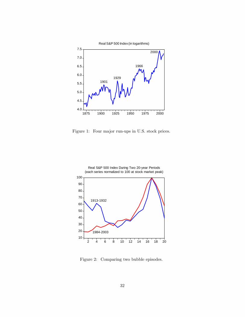
4.0

4.5

5.0

5.5

6.0

6.5

7.0

7.5

1875 1900 1925 1950 1975 2000

Real S&P 500 Index (in logarithms)

19011929

1966

2000

Figure 1: Four major run-ups in U.S. stock prices.

10

20

30

40

50

60

70

80

90

100

2 4 6 8 10 12 14 16 18 20

Real S&P 500 Index During Two 20-year Periods(each series normalized to 100 at stock market peak)

1913-1932

1984-2003

Figure 2: Comparing two bubble episodes.

32

0

10

20

30

40

50

60

70

80

90

1875 1900 1925 1950 1975 2000

S&P 500 Index: Price-Dividend Ratio

Figure 3: The price-dividend ratio reached unprecedented levels around the year 2000.

.024

.026

.028

.030

.032

.034

.036

.038

-.3

-.2

-.1

.0

.1

.2

.3

.4

1996 1998 2000 2002 2004 2006

CBO 4-Qtr Potential Output Growth (left scale) Real S&P 500, Deviation from HP Filter Trend (right scale)

Potential GDP Growth and Detrended Stock Price Index

Figure 4: Rise and fall of the “new economy.”

33

20

40

60

80

100

120

140

1996 1998 2000 2002 2004 2006

Real Business Investment Real S&P 500 Index

Real Business Investment and Real S&P 500 Index(each series normalized to 100 at investment peak)

Figure 5: Comovement of business investment and stock prices.

50

60

70

80

90

100

110

1996 1998 2000 2002 2004 2006

Real Residential Investment Real S&P Case-Shiller Index

Real Residential Investment and Real House Price Index(each series normalized to 100 at investment peak)

Figure 6: Comovement of residential investment and house prices.

34

-1.5

-1.0

-0.5

0.0

0.5

1.0

1.5

2.0

-1.5 -1.0 -0.5 0.0 0.5 1.0 1.5 2.0

Actual Law of Motion for CRRA =1.5Actual Law of Motion for CRRA = 0.1245 degree Line

Act

ual C

oeffi

cien

t fro

m L

aw o

f Mot

ion

Perceived versus Actual Response to Technology Shocks

m = 1.008m = -0.562

0.793

s s

s

---------------------------||||||||||||||

||||||||

Perceived Coefficient Used in Forecast Rule, m

Figure 7: Overreaction to technology shocks tends to be self—confirming.

-2

-1

0

1

2

3

0 400 800 1,200 1,600 2,000

Real Time Learning Paths

Est

imat

ed R

espo

nse

Coe

ffici

ent

Periods

m

m

s

Figure 8: Convergence to the rational solution can be very slow.

35

-40

0

40

80

120

160

0 100 200 300 400 500

Periods

Speculation ModelRational Model

Price-Dividend Ratio

p/d

-40

-30

-20

-10

0

10

20

30

40

0 100 200 300 400 500

Periods

Speculation ModelRational Model

R -1

(per

cent

)

Net Equity Returns

0

2

4

6

8

10

12

0 100 200 300 400 500

Periods

Speculation ModelRational Model

log(

i)

Investment

0

2

4

6

8

10

12

0 100 200 300 400 500

Periods

Speculation ModelRational Model

Consumptionlo

g(c)

0

2

4

6

8

10

12

0 100 200 300 400 500

Periods

Speculation ModelRational Model

log(

k)

Capital Stock

0

2

4

6

8

10

12

0 100 200 300 400 500

Periods

Speculation ModelRational Model

Dividends

log(

d)

Figure 9: Bubbles coincide with economic booms and excess capital formation.

36

-16

-12

-8

-4

0

4

8

12

16

0 10 20 30 40 50 60 70 80 90 100

Periods

Speculation ModelRational Model

Detrended Output

Pct.

devi

atio

n fro

m tr

end

-16

-12

-8

-4

0

4

8

12

16

0 10 20 30 40 50 60 70 80 90 100

Periods

Speculation ModelRational Model

Detrended Consumption

Pct.

devi

atio

n fro

m tr

end

-16

-12

-8

-4

0

4

8

12

16

0 10 20 30 40 50 60 70 80 90 100

Periods

Speculation ModelRational Model

Detrended Investment

Pct.

devi

atio

n fro

m tr

end

-16

-12

-8

-4

0

4

8

12

16

0 10 20 30 40 50 60 70 80 90 100

Periods

Speculation ModelRational Model

Detrended Dividends

Pct.

devi

atio

n fro

m tr

end

Figure 10: Speculation magnifies investment volatility but reduces consumption volatility.

37

-10

-5

0

5

10

15

20

25

0.0 0.5 1.0 1.5 2.0 2.5 3.0

Welfare Cost of Speculation

Wel

fare

Cos

t (p

erce

nt)

theta =0.4

theta=0.6

theta=1.0

Coefficient of Relative Risk Aversion

-10

-5

0

5

10

15

20

25

0.0 0.5 1.0 1.5 2.0 2.5 3.0

Welfare Cost of Business Cycles in Speculation Model

Wel

fare

Cos

t (p

erce

nt)

Coefficient of Relative Risk Aversion

theta=0.4

theta=0.6

theta=1.0

Figure 11: Welfare costs increase rapidly with risk aversion when θ < 1.

38