Embed Size (px)
Citation preview
\STAFF ALLOCATION AND COST ANALYSIS/
APPLICATION OF A HOSPITAL PATIENT FLOW MODEL
by
Richard R. \St. Jean,
Thesis submitted to the Graduate Faculty of the
Virginia Polytechnic Institute and State University
in partial fulfillment of the requirements for the degree of
MASTER OF SCIENCE
in
Industrial Engineering and Operations Research
APPROVED:
OL Wie. Joha/A. White, Chairman
LE Uh Chen. avid M. Cohen
August 1974
Blacksburg, Virginia

5655 V\I55 974 SAF
ACKNOWLEDGEMENTS
The author wishes to express his appreciation to all those who
have contributed to the completion of this thesis.
Special thanks to Dr. John A. White, present chairman of the
graduate committee, and to Dr. David M. Cohen, former chairman of the
committee, currently of the Colorado Foundation for Medical Care,
Denver, for their advice and counsel during the course of this research.
Gratitude is also expressed to graduate committee member Dr. Wayne C.
Turner for his encouragement and advice.
The author extends his appreciation to staff members of the
Montgomery County Hospital, Blacksburg, Virginia for their assistance
in obtaining the data used in this research.
Thanks are extended to Mrs. Janet L. Martin for her excellent
typing of this manuscript.
Finally, the author expresses his deepest appreciation to his
wife, Joanne, for her assistance, patient understanding and constant
encouragement during the graduate study period.
Li
TABLE OF CONTENTS
ACKNOWLEDGEMENTS ° e e « e e * ° e ° e ° e e e e e e e
LIST OF TABLES . . 2... 0 © «© © © © © © eo ew we we we ew ew
LIST OF FIGURES s e e e e es e e ° e e ° e e Cd e . e e e
Chapter
1 INTRODUCTION... 1... 2 ee ee ee eee
Subject of the Research .......24.
Method of Approach . .....-+ +e eeee
Scope and Limitations .......e+ee-e
Survey of the Literature ......+6-.
Forecasting Models ....+4.466-.
Staffing Models ......e «++ eee
Order of Discussion ......624e+2e6-.
MATHEMATICAL STRUCTURE OF THE HOSPITAL PATIENT FLOW, STAFF ALLOCATION AND COST MODELS
Introduction . . . . 2. 2 2 «se we ee ee
The Hospital Patient Flow Model ....
Inputs to the Model ......+sse-.
The Technical Coefficient Matrix ..
The Staff Allocation Model .......-.
Solving the Allocation Model-SUMT ...
The Cost Model... .....2424640e068-s
Summary . « 6 6 « « «© 6 « «
iii
10
10
10
15
18
21
28
31
33
iv
TABLE OF CONTENTS (continued)
Chapter Page
3 RESULTS AND SENSITIVITY . . 1... 2. ee ee ew wee 34
Introduction .... 2... 2 «eee ee eves 34
The Patient Flow Model .......++e.2-e-ee-e 34
The Staff Allocation Model ........2.e666 45
Sensitivity of the Staff Allocation Model .... 63
Use of the Staffing Model .........62ee6 66
Cost Model Results ......4+2+6+40evev-cees 71
Summary 2. 2. 2 6 1 6 6 ew we ee te tt we wt 76
4. SUMMARY AND RECOMMENDATIONS FOR FURTHER RESEARCH .. 78
Summary . 2. 2. 2 6 6 6 6 we we we ew we ee tw 78
Recommendations for Further Study ........ 80
BIBLIOGRAPHY . . . 46 6 we we ee sw we we we we we we ww wh tw te ww 82
APPENDIX A - PATIENT CARE RESPONSE FUNCTIONS .......464s 86
APPENDIX B - PATIENT ADMISSIONS BY CARE-LEVEL TO MONTGOMERY
COUNTY HOSPITAL FROM NOVEMBER 5 THROUGH NOVEMBER 18, 1973 90
APPENDIX C - CARE-LEVEL PROPORTIONS, WARD INDICES AND NURSE
TIME REQUIREMENTS DEFINED FOR NOVEMBER 5 through
NOVEMBER 18 e oo # #8 «@ “ee 8 @*@ >. e@© e© #8 #© © @ #@ @ # @ *o @# @ 95
APPENDIX D - RESULTS OF THE KOLMOGOROV - SMIRNOV TEST WITH
PATIENT ADMISSIONS DATA FROM THE MONTGOMERY COUNTY
HOSPITAL « e# @ # «#8 «@ x e e 68 oo e @ * «© e #© e #© @#© # #@ #© # e@ 100
APPENDIX E - COMPUTER PROGRAM DOCUMENTATION . . e e e ° . . e @ 102
VITA
3.2
3.3
3.4
3.5
3.6
3.7
3.8
3.9
3.10
3.11
3.12
3.13
3.14
3.15
3.16
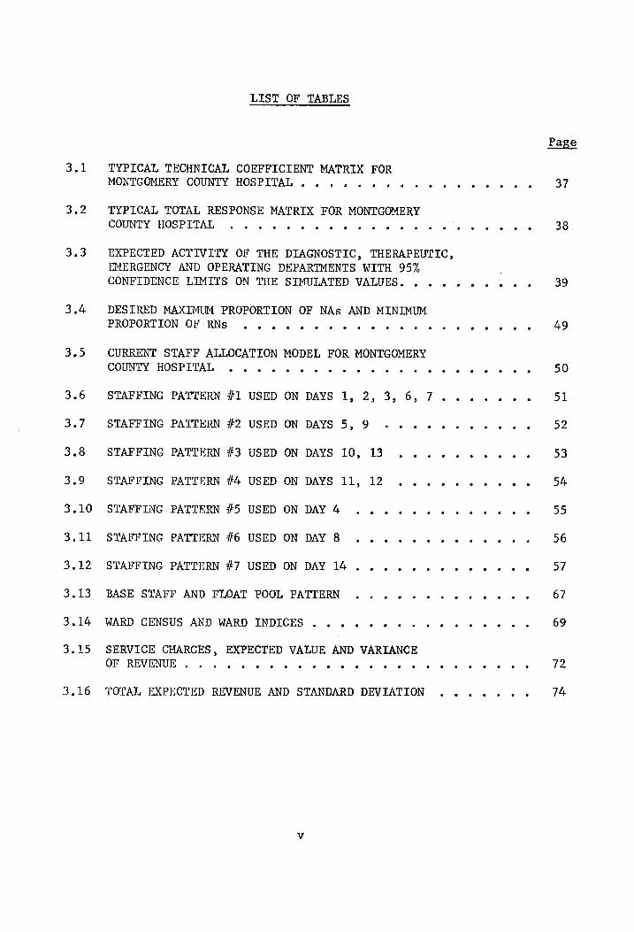
LIST OF TABLES
TYPICAL TECHNICAL COEFFICIENT MATRIX FOR
MONTGOMERY COUNTY HOSPITAL... 4... + «ee.
TYPICAL TOTAL RESPONSE MATRIX FOR MONTGOMERY
COUNTY HOSPITAL . . 1. 1 1 1 6 2 © ee ew ww ww
EXPECTED ACTIVITY OF THE DIAGNOSTIC, THERAPEUTIC,
EMERGENCY AND OPERATING DEPARTMENTS WITH 95%
CONFIDENCE LIMITS ON THE SIMULATED VALUES. ...
DESTRED MAXIMUM PROPORTION OF NAs AND MINIMUM
PROPORTION OF RNs * s ° e o e e e e eo s e ° e
CURRENT STAFF ALLOCATION MODEL FOR MONTGOMERY COUNTY HOSP TTAL ® s e e e » . e ° e e @ e ° e .
STAFFING PATTERN #1 USED ON DAYS 1, 2, 3, 6, 7.
STAFFING PATTERN #2 USED ON DAYS 5,9 .....
STAFFING PATTERN #3 USED ON DAYS 10, 13 ....
STAFFING PATTERN #4 USED ON DAYS 11, 12 ....
STAFFING PATTERN #5 USED ON DAY4 .....
STAFFING PATTERN #6 USED ON DAY 8 .......
STAFFING PATTERN #7 USED ON DAY 14.......
BASE STAFF AND FLOAT POOL PATTERN .......
WARD CENSUS AND WARD INDICES . .....e.s+-eee
SERVICE CHARGES, EXPECTED VALUE AND VARIANCE
OF REV ENUE . e . e e e e e » . s ° e e ° e e e °
TOTAL EXPECTED REVENUE AND STANDARD DEVIATION
38
39
49
50
51
52
53
54
55
56
57
67
69
72
74
2.1
2.2
3.2
3.3
3.4
3.5
3.6
3.7
3.8
3.9
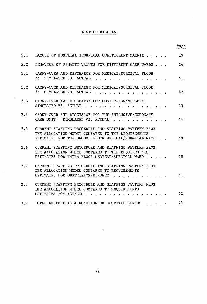
LIST OF FIGURES
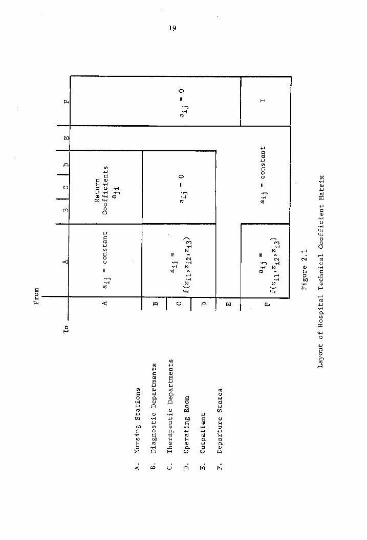
LAYOUT OF HOSPITAL TECHNICAL COEFFICIENT MATRIX .
BEHAVIOR OF PENALTY VALUES FOR DIFFERENT CARE WARDS .
CARRY-OVER AND DISCHARGE FOR MEDICAL/SURGICAL FLOOR
2: SIMULATED VS, ACTUAL ....
CARRY-OVER AND DISCHARGE FOR MEDICAL/SURGICAL FLOOR 3: SIMULATED VS, ACTUAL . .... 6 «© ee «
CARRY-OVER AND DISCHARGE FOR OBSTETRICS/NURSERY:
SIMULATED VS, ACTUAL ...... +646.
CARRY-OVER AND DISCHARGE FOR THE INTENSIVE/CORONARY CARE UNIT: SIMULATED VS. ACTUAL .....
CURRENT STAFFING PROCEDURE AND STAFFING PATTERN FROM
THE ALLOCATION MODEL COMPARED TO THE REQUIREMENTS
ESTIMATES FOR THE SECOND FLOOR MEDICAL/SURGICAL WARD
CURRENT STAFFING PROCEDURE AND STAFFING PATTERN FROM
THE ALLOCATION MODEL COMPARED TO THE REQUIREMENTS
ESTIMATES FOR THIRD FLOOR MEDICAL/SURGICAL WARD .
CURRENT STAFFING PROCEDURE AND STAFFING PATTERN FROM
THE ALLOCATION MODEL COMPARED TO REQUIREMENTS ESTIMATES FOR OBSTETRICS/NURSERY ....e..
CURRENT STAFFING PROCEDURE AND STAFFING PATTERN FROM
THE ALLOCATION MODEL COMPARED TO REQUIREMENTS
ESTIMATES FOR ICU/CCU . .....+ 2 eee e-e
TOTAL REVENUE AS A FUNCTION OF HOSPITAL CENSUS
vi
41
42
43
44
59
60
61
62
75
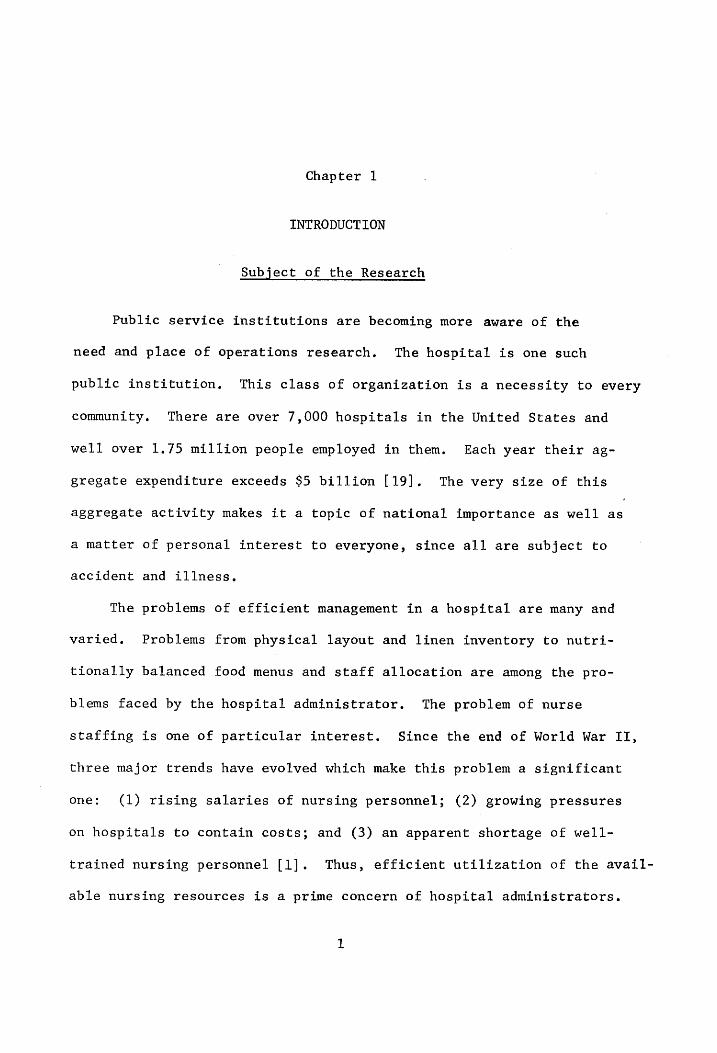
Chapter 1
INTRODUCTION
Subject of the Research
Public service institutions are becoming more aware of the
need and place of operations research. The hospital is one such
public institution. This class of organization is a necessity to every
community. There are over 7,000 hospitals in the United States and
well over 1.75 million people employed in them. Each year their ag-
gregate expenditure exceeds $5 billion [19]. The very size of this
aggregate activity makes it a topic of national importance as well as
a matter of personal interest to everyone, since all are subject to
accident and illness.
The problems of efficient management in a hospital are many and
varied. Problems from physical layout and linen inventory to nutri-
tionally balanced food menus and staff allocation are among the pro-
blems faced by the hospital administrator. The problem of nurse
staffing is one of particular interest. Since the end of World War ITI,
three major trends have evolved which make this problem a significant
one: (1) rising salaries of nursing personnel; (2) growing pressures
on hospitals to contain costs; and (3) an apparent shortage of well-
trained nursing personnel [1]. Thus, efficient utilization of the avail-
able nursing resources is a prime concern of hospital administrators.
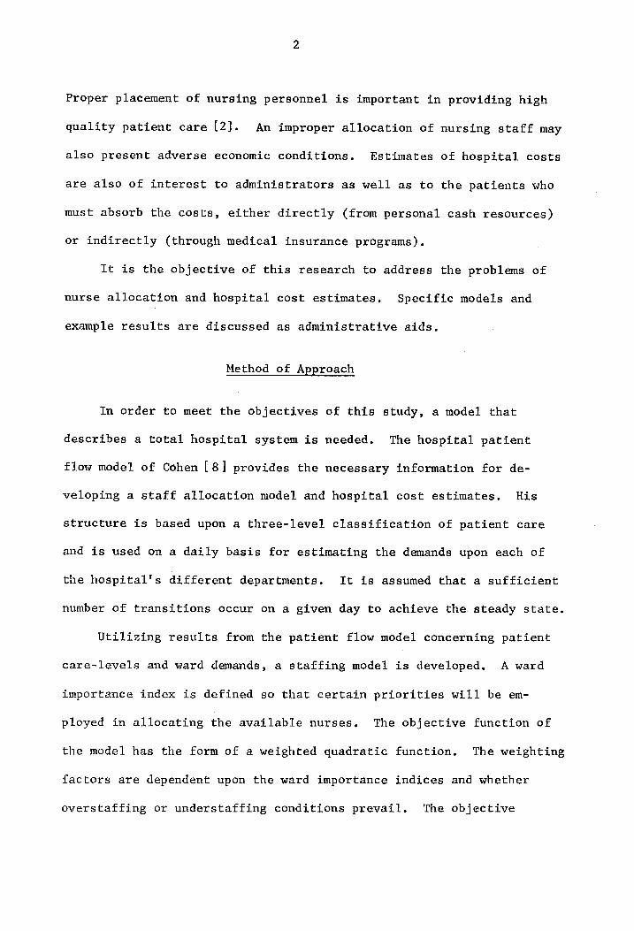
Proper placement of nursing personnel is important in providing high
quality patient care [2]. An improper allocation of nursing staff may
also present adverse economic conditions. Estimates of hospital costs
are also of interest to administrators as well as to the patients who
must absorb the costs, either directly (from personal cash resources)
or indirectly (through medical insurance programs).
It is the objective of this research to address the problems of
nurse allocation and hospital cost estimates. Specific models and
example results are discussed as administrative aids.
Method of Approach
In order to meet the objectives of this study, a model that
describes a total hospital system is needed. The hospital patient
flow model of Cohen [8] provides the necessary information for de-
veloping a staff allocation model and hospital cost estimates. His
structure is based upon a three-level classification of patient care
and is used on a daily basis for estimating the demands upon each of
the hospital's different departments. It is assumed that a sufficient
number of transitions occur on a given day to achieve the steady state.
Utilizing results from the patient flow model concerning patient
care-levels and ward demands, a staffing model is developed. A ward
importance index is defined so that certain priorities will be em-
ployed in allocating the available nurses. The objective function of
the model has the form of a weighted quadratic function. The weighting
factors are dependent upon the ward importance indices and whether
overstaffing or understaffing conditions prevail. The objective
function is minimized subject to constraints on the number of personnel
available by nursing class (registered nurses, licensed practical nurses,
nurses! aids) and on a desirable staffing mix (proportional distribution
of the different nursing classes) for each ward. A sequential uncon-
strained minimization technique provides a heuristic approach for solving
the problem.
The hospital patient flow model,with some results for absorbing
Markov chains,are used for finding cost estimates for the hospital sys-
tem. The example presented assumes constant costs assigned to each of
the hospital's departments.
A model of the Montgomery County Hospital in Blacksburg, Virginia
is formulated as an illustration of the applicability of the models in
a hospital system. Results from a two-week study period provide indi-
cations of the effectiveness of the models.
Scope and Limitations
This research is concerned with the use of a hospital patient
flow model to provide information for the development of a nursing
staff procedure and hospital cost estimates. As is the case in most
mathematical models, every factor related to a hospital system is not
explicitly accounted for in the analyses presented. For example, age
and sex of patients, personal preferences among nurses for their work
stations, and the assignment of private duty nurses to some patients
are not included.
An extensive amount of data is required to achieve an accurate
patient flow model. The Montgomery County Hospital does not store the
necessary information in an easily accessible form. Since only limited
data were available, much of the hospital patient flow model is based
on estimates from the hospital administration. Although confidence in
the results of the model suffered from the lack of sufficient data, an
illustration of the methods was the main consideration. For a detailed
discussion of the stability and sensitivity of the patient flow model
see Cohen [8].
The staffing model presented is aimed at allocating nurses in the
hospital wards. Similar models can be constructed for other types of
personnel or departments found in a hospital.
Survey of the Literature
Over the past fifteen years, considerable research has been done
on various hospital forecasting models and on nurse staffing methods.
The purpose of this section is to present the results of a survey of
the literature. The discussion will involve first the predictive
models and then the staffing methods.
Forecasting Models
Before any type of planning or resource allocation can be per-
formed, some estimates of the requirements is necessary. Thus, to
prepare staff schedules in advance, some prediction of the demands
upon the hospital personnel is needed. Therefore, a review of how
forecasts can be obtained is presented.
Much of the forecasting work has been concerned with predicting
bed needs. Beenhakker [6] devised a multiple regression technique
that takes into account 117 factors which he believes influence 17
classifications of hospital patients. For each of the 17 classifica-
tions, the independent variables most highly correlated with the de-
pendent variable were used in forming the prediction equations. From
the prediction of the number of patients in the hospital for the month,
a forecast of the hospital's bed needs is made.
Another approach that deals with patient classifications for pre-
dicting bed needs is the DPF approach of Blumberg [7]. He groups all
patients of a particular classification into a distinctive patient
facility (DPF). Then, using the finding that arrivals to a DPF are
Poisson distributed, he employs the laws of probability to determine
an optimum number of beds needed in a hospital. Preston et al. [34]
make use of four concurrent surveys on inpatient classifications,
patient classification on a 10% sample of occupied beds, visits to
outpatient clinics, and emergency room visits. Using mean values from
the surveys and a grading system dependent upon patient classification,
bed need estimates are made for planning new facilities. The problem
of bed allocation is also addressed by Jackson [24]. His approach is
the minimization of a penalty associated with patients not being ad-
mitted to the necessary or desired service. A queuing model is used
in determining the number of patients turned away from a service.
Queuing theory has also been applied to various sectors of the hospital,
such as operating room, delivery room, and outpatient facilities
{42} [44] [51].
Purcell [38] investigated self-adaptive forecasting models for
use in predicting health service demands. Twelve different models
were tested against actual staff admissions and ranked according to
average squared error. Admissions have been treated in other studies
with regard to scheduling [12] [27] [39].
Balintfy [3] has formulated a patient census predictor model which
uses hospital length of stay with a Markovian model. The patient flow
model of Cohen [8] is also a Markovian type model, His model provides
the patient load to each of a hospital's departments. This predictive
model was chosen for use in providing information for the staffing and
cost models. Further discussion of the model is presented in Chapter 2.
In reviewing the literature on hospital forecast studies, several
common characteristics were observed. One finding that is consistent-
ly utilized is that patient admissions to various hospital sectors are
Poisson distributed. Another common feature of many of the predictive
models is that they are designed for monthly or annual study periods.
Staffing Models
In the staffing literature, much similarity is again found on many
points. Nursing load factors are often discussed for each ward. Pa-
tients are commonly classified into self, intermediate, and intensive
care categories. The decision rules for the classification of patients
are also quite similar. A relative weighting between care-levels is
usually assigned. These weights are generally the same: intermediate
has twice the weight of self care, and intensive has five times the
weight of self care. The factors are derived from the direct nursing
care given to each classification. The time differences are supported
by a work sampling study done by Connor [9] [10]. The ward loads are
then calculated by summing the weighted number of patients by care-
level in each ward. Staffing assignments are then to be performed
with this index as a guide. The work of Barr [5], Connor et al. [11],
Flagle [19], Holbrook [22], Ryan and Boyston [40], Wolfe and Young
[50], and Price [35], all follow this similar pattern.
Wolfe and Young address a constrained staffing problem. The
common studies involve deriving an index and concluding that staffing
Should be done accordingly. However, a ward index alone may not aid
in making the best staff allocation of available nurses. To solve
this problem, Wolfe and Young have developed a multiple assignment
model. Their model uses a subjective cost, in dollars, for each com-
bination of 16 tasks and the costs of having six different personnel
classes perform them. They minimize the hospital's value cost (a sub-
jective value) with the number of each personnel type available as
constraints.
Warner and Prawda [46] also have addressed the nursing staff
allocation problem. They define a mixed-integer quadratic programming
problem to minimize a "shortage cost."' Parameters needed by the
model include nursing hour requirements, weighting factors of rela-
tive seriousness for deviating from requirements and substitutability
estimates among the different nursing levels for each shift of a
Study period. Costs of overstaffing are assumed to be zero.
As with the predictive models, there were common interesting points
found in the staffing literature. Nearly all the authors agree that
patient load and not census is the important factor to consider. They
report instances where variation in load index is not the same as the
variation in census, in magnitude or direction. Wide fluctuations in
ward loads and daily variation among them are reported as general hos-
pital characteristics. It is noted that by pooling all wards together,
the daily vacillation diminishes significantly. To achieve a pooled
effect, a method called controlled variable staffing is recommended.
This method designates some minimum base staff to each ward and places
the remaining personnel into a float pool. The pooled nurses may
then be directed to different nursing stations according to the pa-
tient load. After some period of adjustment, a controlled variable
staffing procedure has worked satisfactorily at the Montana Deaconess
Hospital [22].
Most authors report that a usual procedure in hospitals is to staff
for peak loads. But peak loads are rarely near the average work load
and the result is a highly trained, highly paid nurse who is idle 20%
to 35% of the time.
This review of hospital studies provides some insight into the
methods currently available to hospital administrators for making
demand predictions and nurse allocations. While demand forecasts are
needed in the staffing models, no direct links to specific predictive
models have been shown. One of the primary purposes of this research
is to show how information from a specific predictive model can be
utilized to perform staffing and cost studies.
Order of Discussion
The results of the research are presented in the following format:
Chapter 2 provides the mathematical formulations of the hospital

patient flow model, the staffing model and cost estimation procedures;
results obtained from applying the models to Montgomery County Hospital
are presented in Chapter 3; and Chapter 4 contains a summary of the
research and a listing of recommendations for further study.
Chapter 2
MATHEMATICAL STRUCTURE OF THE HOSPITAL PATIENT FLOW,
STAFF ALLOCATION AND COST MODELS
Introduction
In the previous chapter, it was mentioned that a hospital patient
flow model can be used to predict the demands upon the various hospital
departments. It is the purpose of this research to illustrate how
staffing and cost models can be formed from the information provided
by the patient flow model. This chapter presents the mathematical
structure of the models to be used. A discussion of the patient flow
model is presented first, followed by the staffing and cost model
formulations.
The Hospital Patient Flow Model
In modeling hospital patient flows, the input-output model de-
veloped by Cohen [8] will be used. Since the staffing and cost models
to be presented utilize many of the concepts from the patient flow
model, a brief discussion of the model is presented.
A hospital can be divided into a number of sectors. In a general
hospital, the sectors can be classified into several broad categories,
including:
(a) Nursing Stations
10
11
(b) Diagnostic Departments - e.g., X-Ray
(c) Therapeutic Departments - e.g., Physical Therapy
(d) Operating Room
(e) Outpatient - Emergency Room
A patient's transfer behavior among the various sectors can be repre-
sented by a matrix of technical coefficients, with the row i, column j
entry denoting the proportion of patients in sector j who transfer di-
rectly to sector i of the hospital on a given day. Thus, each technical
coefficient can be interpreted as the probability of a patient trans-
ferring from, say, sector j to sector i ona given day. The values of
the technical coefficients, or transition probabilities, can be related
to various levels of patient care. In this study, three levels of care
are considered: self, intermediate and intensive. The rules given by
Barr [5] are employed in categorizing patients by care-level.
Additional sectors will be added to the model to reflect the
output areas from the system. The new sectors can be categorized as
follows:
(a) Discharged patients
(b) Deceased
(c) Carry-over patients
A technical coefficient matrix is formed by augmenting the original
matrix of technical coefficients with the appropriate technical co-
efficients for the output sectors. The new technical coefficient
or transition probability matrix assumes the structure of an absorbing
Markov chain [14] [23] [26] [43] [47].
In a Markov chain process, there is a given set of states and
12
the process can be in only one of these states at a given time. The
process moves successively from one state to another. A probability
of transition from one state to another is assigned for every ordered
pair of states. The probability that the process moves from some state
j to state j is dependent only on the state j that it occupied before
the step. An absorbing Markov chain contains at least one state from
which it is impossible to leave. It must be possible to go to an ab-
sorbing state in one or more steps from every nonabsorbing state in
an absorbing Markov chain.
Each of the hospital sectors can be considered a state of the
Markov chain. Since a patient cannot be in two sectors at once, he
can be in only one state at any given time. The technical coefficients
matrix provides the probability of transition from one sector to an-
other. The output sectors can be called the absorbing states. Once
a patient has been discharged or assigned for carry-over, he is no
longer available for transfer to other hospital sectors. Note,
that since a carry-over sector is added to the technical coefficient
matrix, the probability that a patient transfers from a given sector
into the same sector is zero. In other words, the transition proba-
bilities from sector j to sector j are zero for the nonabsorbing, or
transient sectors.
Some results for absorbing Markov chains can now be used to find
certain estimates concerning a hospital's flows. A matrix giving the
expected number of times a patient enters a sector i, given he started
in sector j on day (t) is given by:
wht) = cq — alt)y-1 (2.1)
where
not) =
A(t) =
H It
Ss
13
8 x S matrix of expected number of times a patient enters
sector i, given starting sector j on day (t).
s x s matrix of technical coefficients on day (t).
s x s identity matrix.
the number of hospital sectors, excluding output sectors.
The matrix N‘t) will be called the total response matrix. In order
to find the expected number of patients passing through a sector on
a given day, the total response matrix is multiplied by a vector con-
taining the number of patients entering the hospital on that day. In
mathematical notation:
where
x(t)
y(t) =
c(t-1)
In order to
x(t) 2 y(t) y(t) 4 g(t-1)) (2.2)
s-vector whose elements are the expected number of patients
entering each sector on day (t).
s-vector whose elements are the number of admissions to
each sector on day (t).
S-vector whose elements are the number of carry-over
patients from day (t-1l).
give more meaning to the expression for the expected num-
ber of patients entering a sector on a given day, a derivation of
Equation 2.2 is presented.
The expected number of patients entering a sector on a given day
includes the number of new admissions to the sector, the patients in
the sector that were carried over from the previous day and the number
of patients who transfer into the sector from the other hospital sectors.
14
Expressed in mathematical form:
x, 6t) = 424 adj (t) x, (t) + yz St) + cy (t-1) (2.3)
i=l, 1s
where
x, 6t) = the expected number of patients entering sector i on
day (t).
a; ; 6) = probability of transfer from sector j to sector i during
day (t).
y4 60) = the expected number of new patients admitted to sector
i during day (t).
c, (t-1) = the expected number of patients in sector i on day (t-1)
who remain in sector i on day (t).
Recall that ayy is zero for each of the hospital sectors. Equation
2.3 can be written in matrix notation as follows:
x(t) = alt)y(t) 4 y(t) + ¢(t-1) (2.4)
where x(t) , y(t) | and c(t~1) are s component column vectors and a(t)
is ans x s matrix of technical coefficients.
To solve for x(t) in Equation 2.4, the quantity A(t)y(t) is sub-
tracted from both sides of the equation and becomes
(I — A(t)yx(t) = y(t) + c(t-1) (2.5)
where I is an s x s identity matrix. Premultiplying both sides of
Equation 2.5 by the inverse of the matrix (I - A(t)), which is nt)
of Equation 2.1 gives the desired result of Equation 2.2.
Thus, given the number of patients admitted to the hospital along
with the number of patients carried over from the previous day and a
matrix of technical coefficients, the expected number of patients
15
entering each sector of the hospital can be predicted. The two major
components of the patient flow model, the input vectors and technical
coefficients matrix, will now be discussed in further detail.
Inputs to the Model
The new admissions and the carry-over patients are considered
separately as the input factors to the model. Both input factors take
patient care-levels into consideration.
For short term purposes, the hospital would probably have a list
of patients who have appointments to enter. The preliminary diagnosis
of a patient's condition can be used to estimate which level of care
he will be requiring. It is assumed that the hospital has its own
procedure for scheduling elective patients. If a scheduling method
is not employed, experience with the patient flow model may be helpful
in establishing one, since the hospital's occupancy levels can be pre-
dicted. Several scheduling techniques are also mentioned in the lit-
erature [12] [25] [39].
The number of unscheduled patients entering the hospital on a
given day is not found quite so simply. In order to provide some es-
timate of the number of patients that enter the hospital system un-
scheduled, one of the forecasting models discussed in Chapter 1 could
be employed.
The following notation will be used to represent new admissions
to each of the hospital sectors on day (t).
t
where
16
y;‘t) = the total number of new patients admitted to sector i
on day (t).
yik(t) = the number of new patients admitted to sector i on
day (t) who are in care-level k.
k = 1 designates self care.
k = 2 designates intermediate care.
k = 3 designates intensive care.
From the patient flow model of the previous day, the number of
carry-over patients can be found. Results for absorbing Markov chains
will again be employed. From a matrix of the technical coefficients
for the departure sectors, or absorbing states, and the total response
matrix, y(t) | a matrix that gives the probability of a patient depart-
ing in sector i, given that he began in hospital sector j, can be *
defined as follows:
p(t) = p(t)y(t) (2.7)
where
B(t) = r x gs matrix of probabilities of departure through sec-
tor i, given starting sector j on day (t)
R(t) =r x s matrix of technical coefficients from the hospital
sector j to the departure sector i on day (t).
the number of departure sectors. r
Thus, elements of matrix ptt) corresponding to the carry-over sector
can be used in finding the estimated number of patients carried over
to the next day. Suppose row k designates the carry-over row of
matrix Bit) | then the following equation is used to obtain the
expected number of carry-over patients for sector j on day (t):
17
.
c,(F) = a4. (E) (0, 6E° 4) + v4") (2.8)
where
_(t) = the probability that a patient who began in sector j is
carried over (is absorbed in the carry-over sector k) on
day (t).
c (t) _ the expected total number of patients carried over in
sector j on day (t).
Equation 2.8 gives no indication of the number of carry-over pa-
tients in each care-level. Itwill be assumed that the proportion of
carry-over patients remains the same as the proportion of patients in
each care-level that entered the sector on a given day [8] [50].
Therefore, care-level proportions needed for each day are found from:
vig? + 04, 6E)) zin(®) = ap (2.9)
Yi FG
where
z 4460) = the proportion of patients input to sector i in care-
level k on day (t).
cy ft) = the expected number of carry-over patients for sector i
in care-level k from day (t-1l).
Now to obtain the number of patients expected to be carried over on
day (t) by care-level, the following expression is used:
ci, 6t) = 0; (t)2,, CE) (2.10)
The inputs required to use the hospital patient flow model in-
clude the number of new admissions and the number of carry-over
patients from the preceding day. Since the carry-over estimates are
18
generated from the model and the number of elective admissions are
known in advance, only a forecast of the number of unexpected arrivals
need be performed for employment of the hospital patient flow model.
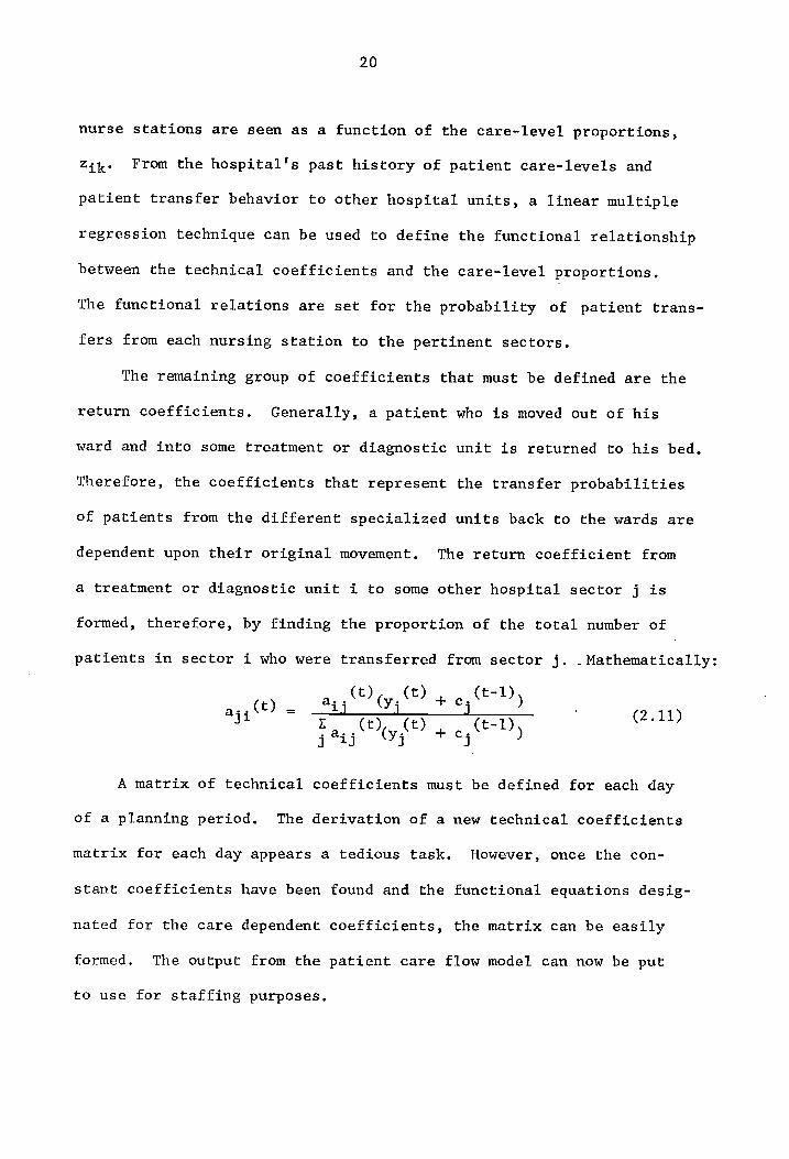
The Technical Coefficient Matrix
In Cohen's work [8], the technical coefficients were not all
formulated in the same manner. Some coefficients were found to be
constant, some depended on care-level proportions, and another group
was influenced by other technical coefficients. Figure 2.1 gives the
basic matrix layout for a day.
From the figure, it is seen that transfers between the nursing
stations are constant. The proportion of patients going from the
outpatient areas to other hospital sectors is also constant. Also,
patients moving from nursing stations to outpatient are unchanged.
Furthermore, values for patients moving to outpatient or departure
categories from the diagnostic units, therapeutic units and operating
room are constantly proportioned. Zero coefficient values are found
in the matrix. There are obviously no transfers taking place from
the departure categories. It is also assumed that patient movement
among the diagnostic units, therapeutic sectors, and operating room
does not occur. Thus far, the values of the matrix have had a static
nature for any given day. The remaining values of the technical coef-
ficient matrix will be dependent upon the patient care classifications
for the day.
In Figure 2.1, the technical coefficients for patients entering
diagnostic, therapeutic, operating and departure sectors from the
XTAJEW
JUSTOTFJFI0N
[eotuyoay
[eqrdsoy
jo ynokey
19
qd
| oO
d
T°Z eansty
queqsuoo
= fTe
= {Ip
qd
Cto<«¢cto< Tt
Ct (ez
z Z)J
OoO- °7e
c 9
= tle
q
Te,
SJUSTITF F909
jue SUOD
= [T.
uinjsy
V
woi7
OL
sa3eqsg eanjaedaq
quatjeding
Wooy
But erzsedg
Sjueujiedeq
oT4nadezayy
Sjusujziedsq
sTJsoUusetg
suotjeqsg
Bursany
20
nurse stations are seen as a function of the care-level proportions,
Zi From the hospital's past history of patient care-levels and
patient transfer behavior to other hospital units, a linear multiple
regression technique can be used to define the functional relationship
between the technical coefficients and the care-level proportions.
The functional relations are set for the probability of patient trans-
fers from each nursing station to the pertinent sectors.
The remaining group of coefficients that must be defined are the
return coefficients. Generally, a patient who is moved out of his
ward and into some treatment or diagnostic unit is returned to his bed.
Therefore, the coefficients that represent the transfer probabilities
of patients from the different specialized units back to the wards are
dependent upon their original movement. The return coefficient from
a treatment or diagnostic unit i to some other hospital sector j is
formed, therefore, by finding the proportion of the total number of
patients in sector i who were transferred from sector j. . Mathematically:
(tt), (t) (t-1) a(t) 2 947 Ot ) ji r
j
2.11 ay UM + eg ED) (2.1)
A matrix of technical coefficients must be defined for each day
of a planning period. The derivation of a new technical coefficients
matrix for each day appears a tedious task. However, once the con-
stant coefficients have been found and the functional equations desig-
nated for the care dependent coefficients, the matrix can be easily
formed. The output from the patient care flow model can now be put
to use for staffing purposes.
21
The Staff Allocation Model
In the previous section, a hospital patient flow model was discussed.
A prediction of the total number of patients expected to be treated in
each of the hospital sectors can be found from the model. The patient
flow model forecasts can now be used for staffing purposes. The major
concern here is the development of a nurse staffing procedure for the
wards. However, other staffing procedures may be formulated along simi-
lar lines for other hospital departments.
The number of patients expected to be treated in a ward is not
the same as the ward census. The ward census gives the number of beds
occupied in the ward at a specific time of the day. The number of
patients expected to be treated, or the total activity, in a given ward
on a day can be considered as a counter for every patient transfer into
the ward. This means that some patients are counted more than once.
For example, suppose a patient must leave the ward to have X-rays
taken. Upon his return, he is counted as a new patient transferred
into the ward. It is reasonable to staff according to a ward's total
activity, since every patient transfer requires more nursing attention
than for a patient who remains in his bed. When a patient must be
transferred to another hospital unit, preparation of the patient,
actual transportation or assistance to the patient, resituation and
updating of his chart are usually performed by some level of the
nursing staff. The specific preparations for a patient's transfer
are also dependent upon his care-level. A person being treated for
a broken wrist and a patient just recovering from major surgery would
not need the same type of transfer consideration. Therefore, the
22
total activity vector, x(t) must be broken down into care-levels.
Recall that Equation 2.9 defined the proportion of care-levels
for each of the ward areas. Because the technical coefficient matrix
gives a proportion of transfers for any entry into the specific sector,
patients in different care~levels are treated identically. Therefore,
the percentage of patients in each care classification are the same
in the total activity vector as in the original input state. Thus,
to find the number of patients of each care-level that are expected
to enter a given sector, Equation 2.12 can be used.
by ft) = x, C625, C8) (2.12)
where
bi, = the expected number of patients in care-level k entering
sector i on day (t).
Now, with an estimate of the number of patients expected in each
ward by care-level available, some estimate of the nursing time re-
quired to adequately care for the patients can be made. The nurse
requirements are a function of the number of patients in each care-
level expected in the ward on a givenday. The requirements estimate
is in terms of the number of nurses working a full 8-hour shift.
a ft) o (t) (t) (t) i bigs Bag) (2.13)
where
R, St) = estimate of nursing time requirements for ward i on
day (t), measured as the number of nurses working
8-hour shifts.
g (by, *)) some function that provides the nursing time requirements
23
using the expected number of patients entering ward i
by care-level on day (t).
The objective now is to schedule the nursing staff as close
as possible to the estimated nursing time requirements. However,
because of fluctuations in daily workload and the likelihood that R, (t)
will imply fractional nurse days, an attempt to schedule staff strictly
adhering to the estimate would probably meet with considerable diffi-
culty. Also, a fixed nursing staff is usually available on a given
day. The question of where any extra staff should be placed or, if
all requirements can't be met, which ward should suffer the personnel
shortage is not answered. Thus, the allocation model will take over-
staffing and understaffing factors into consideration.
In the construction of the ward staffing model, utilization
of the requirements estimates, R, (t), and the care-level proportions,
zat will be made. Another concept that will enter the design is
one of ward rating. In other words, a priority system will be devised
in order to allow the more critical areas an advantage in the staffing
procedure.
Barr [5] developed an index by weighting the number of patients
in each care classification and summing them. However, his index was
used more as a requirement standard than as a rating for the wards.
The number of patients in absolute terms is not needed for rating here,
since a nurse time requirement has already been established. Rather,
the ward will be rated solely according to the types of patients it
handles. The care proportions for each unit will be used for rating
purposes. The ward importance index will be defined as follows:

24
(t) _ (t) Wy = Zi1 + 2249 (1) 4 5244 (2.14)
where w; &t) = ward index for sector i on day (t).
The weighting values of 1, 2, and 5 are assigned based upon the
ratio of time generally spent among the patients of the different care
classes. Thus, each ward will have an index valued between 1 and 5.
A value of 5 indicates an entirely intensive care ward, and therefore,
will have top priority as to meeting its needs in the staffing model.
At the opposite extreme, a value of 1 indicates a completely ambula-
tory ward and the procedure will give it a low priority.
Now, an objective function for the staffing model is defined.
The value of the objective function can be thought of as a penalty
for staffing either above or below the predicted requirements level.
The desire is to allocate personnel so as to minimize such penalties.
The objective function takes on values based on the ward index and
the magnitude of the difference between the staff allocation and the
requirements estimate. The staffing model takes the following form:
min Fp, (t) (Rr, (&) - n, (t))? (2.15)
where
w, 6 n, 6? < R, ©
t) . P, | (t) (t) (t)
L/wy ny > Ry
n, 6° = number of nurses assigned (8-hour shifts) to sector i
on day (t).
p, ©) = penalty value for ward i on day (t)
25
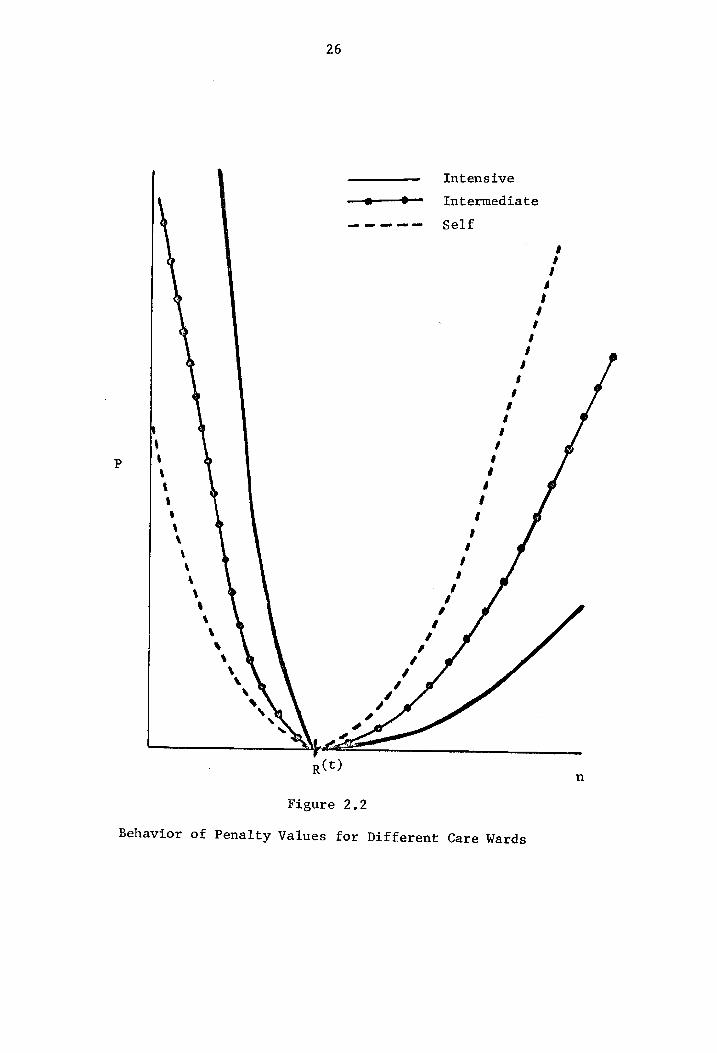
The makeup of the objective function indicates that overstaffing
and understaffing receive different treatment in the model. The ob-
jective functions found in the literature review in Chapter 1 did not
use the switching concept. One type of objective function penalized
understaffing only, with zero being assigned to the overstaffing case.
The other type objective functions attempted to minimize some subjective
cost of not satisfying the demand requirements exactly, without regard
to whether overstaffing or understaffing is the case. The objective
function of Equation 2.15 provides a penalty assignment for overstaffing,
but a lesser penalty than one incurred for understaffing.
As illustrated in Figure 2.2, the ward index plays a substantial
role in the model formulation. Notice that the penalty curve is de-
pendent upon the ward index. When an understaffing condition is pre-
valent, the intensive care unit incurs the greater penalty. But once
the equilibrium point, R(t), is passed and overstaffing is the situ-
ation, the graph indicates that intensive care wards will be penalized
to a lesser degree than the lower ranking units. The staffing model
is designed in this manner so that if extra staff time is available,
it should be placed in the more critical areas of the hospital.
To this point, constraints to the system have not been mentioned.
The unconstrained solution to Equation 2.15 is obviously R, (t), for
each i, where the penalty becomes zero. But since R, 6) changes over
t and may generally contain fractional parts of a work day, staffing
at exactly those levels would not be practical. The model to be pre-
sented here will allocate theavailable staff for each time period and
maintain a desired balance among the personnel for each ward.
26
————— ee Intensive
—@e—-e— _ Intermediate
— wep a em eh Self
R(t)
Figure 2,2
Behavior of Penalty Values for Different Care Wards
27
The nursing staff in a hospital can be divided into three dif-
ferent levels: registered nurses (RN), licensed practical nurses
(LPN), and nurses’ aides (NA). Because each level possesses dif-
ferent skills, generally a specific mix of the nursing staff for
each ward is desired. Some minimum proportion of each ward's nursing
staff should be RNs, since they are the most highly trained. On the
other hand, there should be limiting factors on the proportion of
NAs assigned to a ward. Therefore, constraints concerning the staff-
ing mix in a ward are necessary to the allocation model.
The hospital has available a specific number of nurses in each
skill category who usually expect to work a full day. The staffing
model will, therefore, specify integral assignment. With the use of
integral assignment and because of the available levels of nursing
staff, the possibility of meeting the staffing mix guidelines for each
ward may be diminished. However, the staffing model should make use
of the available number of RNs, LPNs, and NAs present on a given day
to meet the demands of each ward maintaining some staff mix as closely
as possible.
Equation 2.15 is now reformulated to take into account the dif-
ferent classes of nurses. A switching variable, §, is added to control
the proper weighting for understaffing and overstaffing situations.
Constraints on the number of nurses available are added. The minimum
acceptable proportion, Y;, of RNs and a maximum proportion, 8;, of NAs
desired for each ward are also added as constraints. The mathematical
representation of the staffing model for each day t is:
min ;
8; (wy2-1) + wy? +1 i i (wi" 1) * Wi (Ry-(qq + ry + s;))* (2.16)
2wy

28
subject to: 2 qy = Npn
y = N ¢ Ti LPN
y = N Si NA
(1 -yz)qa - yi(ry + sy) > 0
By (ay + ry) - (1 -B;)s; > 0
6, _ Fs t [Ry - (qq + ry + si) |
- (q; + Tr; + s,)
dj> zy, 84, all integer, for all i.
Nen = the number of RNs available on a given day.
Nupyn = the number of LPNs available on a given day.
Nya = the number of NAs available on a given day.
qi = the number of RNs assigned to ward i.
a = the number of LPNs assigned to ward i.
Sy = the number of NAs assigned to ward ti.
O4 = variable that controls the weighting factor, depending
on whether the staff allocation to a specific ward is
greater than or less than the requirements estimate.
Yq = the minimum proportion of the nursing staff that are
RNs desired in ward i.
By = the maximum proportion of the nursing staff that are
NAs desired in ward i.
solving the Allocation Model -— SUMT
The staffing model as defined above is a nonlinear programming
problem with linear and nonlinear constraints. Sequential uncon-
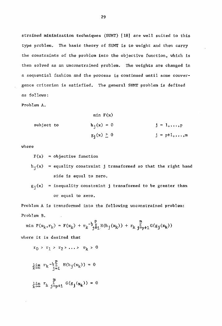
29
strained minimization techniques (SUMT) [18] are well suited to this
type problem. The basic theory of SUMT is to weight and then carry
the constraints of the problem into the objective function, which is
then solved as an unconstrained problem. The weights are changed in
a sequential fashion and the process is continued until some conver-
gence criterion is satisfied. The general SUMT problem is defined
as follows:
Problem A.
min F(x)
subject to hy (x) = 0 j = 1,...,p
g,(x) 2 0 j = ptl,...,m
where
F(x) = objective function
h(x) = equality constraint j transformed so that the right hand
side is equal to zero.
8; (x) = inequality constraint j transformed to be greater than
or equal to zero.
Problem A is transformed into the following unconstrained problem:
Problem B.
1, PB . . _ . : min P(x,,r,) = F(x,) + Tye *524 HC y 4.) + Tye jz yey F(85 CX)?
where it is desired that
Yo > Ty > To> eee > Ty > 0
1
: iP im ry, “22 ->00 j=
m i y Ge. = 0 im rk jzptl (8; (x,)) 00 +
30
jim | P(x, »r,) - F(x, )| = 0
and, H(h (x,)) and G(g 5 (x,)) are transformations upon the equality and
inequality constraints, respectively.
In order to guarantee convergence to the optimum, one criterion
is that the equality constraints be linear. This condition is not
satisfied in the staffing model. However, SUMT can be used as a
heuristic approach which may in many cases yield good results. In
fact, the method worked very well for the problem defined in Equation
2.16.
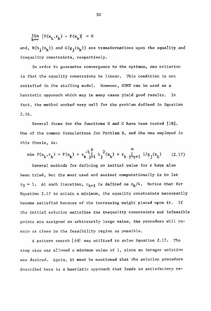
Several forms for the functions H and G have been tested [18].
One of the common formulations for Problem B, and the one employed in
this thesis, is:
rer: . min P(x Ty = F(x, ) + ry jel h, (x,) +r, jep+l 1/8 (x) (2.17)
Several methods for defining an initial value for r have also
been tried, but the most used and easiest computationally is to let
rg = 1. At each iteration, r,,) is defined as r,/4. Notice that for
Equation 2.17 to attain a minimum, the equality constraints necessarily
become satisfied because of the increasing weight placed upon it. If
the initial solution satisfies the inequality constraints and infeasible
points are assigned an arbitrarily large value, the procedure will re-
main as close to the feasibility region as possible.
A pattern search [49] was utilized to solve Equation 2.17. The
step size was allowed a minimum value of 1, since an integer solution
was desired. Again, it must be mentioned that the solution procedure
described here is a heuristic approach that leads to satisfactory re-
31
sults for the staffing model of Equation 2.16.
The Cost Model
In the section on the hospital patient flow model, it was remarked
that the technical coefficient matrix functions as an absorbing Markov
chain. Consequently, several results for absorbing Markov chains given
by White [47] can be employed in estimating certain hospital revenues.
In order to be consistent with the notation used by White, the trans-
pose of the technical coefficient matrix, a(t) | will be denoted as g(t),
The expected revenue that each hospital department generates is
an example of information that can be gained from the hospital patient
flow model. With knowledge of the expected revenue, the hospital ad-
ministrator can evaluate his budget decisions for the various depart-
ments. He could also test the effects of a change in charges for
various hospital services. Information concerning the hospital's
expected revenue, therefore, can be very useful in formulating the
budget and cost policies of the hospital.
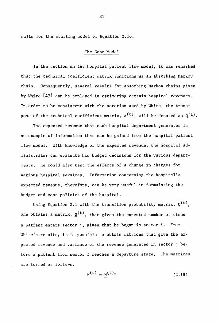
Using Equation 2.1 with the transition probability matrix, g(t) |
one obtains a matrix, nCt) | that gives the expected number of times
a patient enters sector j, given that he began in sector i. From
White's results, it is possible to obtain matrices that give the ex-
pected revenue and variance of the revenue generated in sector j be-
fore a patient from sector i reaches a departure state. The matrices
are formed as follows:
m6t) . ylOde (2.18)
where
ft)
t)
Ss
Sdg
32
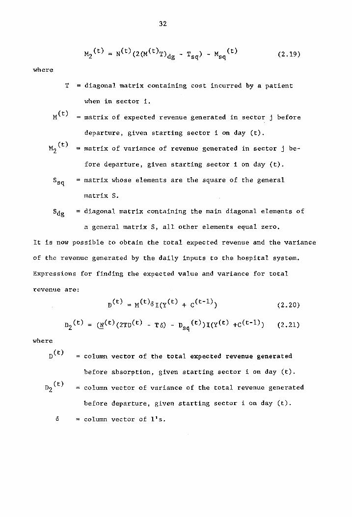
My(t) = nw) (2a 7) a, - Tyq) - Mog’ (2.19)
diagonal matrix containing cost incurred by a patient
when in sector i.
matrix of expected revenue generated in sector j before
departure, given starting sector i on day (t).
matrix of variance of revenue generated in sector j be-
fore departure, given starting sector i on day (t).
matrix whose elements are the square of the general
matrix §.
diagonal matrix containing the main diagonal elements of
a general matrix S, all other elements equal zero.
It is now possible to obtain the total expected revenue and the variance
of the revenue generated by the daily inputs to the hospital system.
Expressions for finding the expected value and variance for total
revenue are:
pot) = wfsreyOt) 4 clE-D) (2.20)
DCF) = (nCE) (2rpCt) - 79) - dog 6 )t¢xC@) +c€@-P)) (2,21)
where
pot)
pp (t)
column vector of the total expected revenue generated
before absorption, given starting sector i on day (t).
column vector of variance of the total revenue generated
before departure, given starting sector i on day (t).
column vector of 1's.
33
Results from the patient flow model and cost model can be used
to predict estimated revenue for budgeting purposes, to examine the
effects upon revenue of changes in service rates and to find the re-
lationships of various departments to the total revenue structure.
Additionally, the sensitivity of total revenue produced to changes
in the care-level distribution of patients can be studied using
Equation 2.18 thru 2.21. Finally, the same equations can be used
to model the consumption of other resources such as food, linens, and
medicines by appropriately modifying the resource matrix T.
Summary
This chapter has presented several mathematical models that can
be used as an aid to a hospital administrator. First, a hospital
patient flow model that is capable of predicting departmental demands
was discussed. A staffing model was then developed using the pre-
dicted ward demands and a ward rating system. Finally, some results
for absorbing Markov chains that can be used to find the revenue gen-
erated in each hospital sector were presented. The next chapter
provides results obtained from the models for the Montgomery County
Hospital.
Chapter 3
RESULTS AND SENSITIVITY
Introduction
To provide an illustration of the models developed in Chapter 2,
assistance from the Montgomery County Hospital in Blacksburg, Virginia
was enlisted. A hospital patient flow model was designed to represent
the Montgomery County Hospital. Information on a desirable staff mix
for the different wards was obtained and the staff allocation model
given in Chapter 2 was tested, using results from the patient flow model.
The patient flow model was also used to provide an expectation of the
revenue generated for the study period.
This chapter will illustrate the application of the models discussed
in Chapter 2. The hospital patient flow model for the Montgomery County
Hospital is presented first. Results from the staff allocation model
are then provided, along with several comments on sensitivity and imple-
mentation. One final section gives results from the utilization of a
cost model with the hospital patient flow model.
The Patient Flow Model
The Montgomery County Hospital is a relatively small 100 bed
hospital and is a member of the Hospital Corporation of America. Data
were gathered on patient admissions, discharges, and the staff levels
34
35
allocated to the various wards for a two week period in early November
1973. Much of the other information needed to develop the technical
coefficient matrices were not readily available or were contained in
confidential records. Patient names and diagnoses, which are also
kept confidential, were required for defining the proper care-levels.
Since information was limited, much of the technical coefficient matrix
is based upon estimates from the hospital staff. Obviously, much more
data should be used when determining a model of this type. However,
the main emphasis in this thesis is not to revalidate the application
of complex linear flow models to a hospital system, but rather it is
to illustrate uses of the model in performing staff allocation and cost
studies. Thus, a patient flow model was developed with the available
data and estimates.
Ten sectors and two absorption states were defined for the Mont-
gomery County Hospital. Nursing stations included two medical/surgical
wards, a combined intensive and coronary care unit, and an obstetrics
ward with nursery. Diagnostic departments were EKG, Laboratory, and
Radiology. A Physical Therapy section, Operating Room, and Emergency
Room complete the ten hospital sectors. The absorption states were
discharge and carry-over.
Where enough data were available, patient care-level response
functions, £ (2445) 2456), 2346), were developed using a linear
multiple regression technique. The care-level functions for the two
medical/surgical wards can be found in Appendix A. Adding constant
coefficients based on estimates, and forming return terms as discussed
in the previous chapter, a matrix of technical coefficients was de-
36
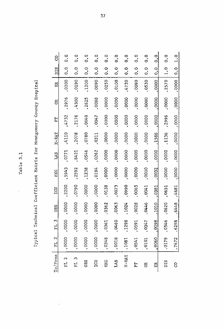
fined in a form similar to that of Figure 2.1. The constant terms were
defined for each day of the week. A typical technical coefficient matrix
for the Montgomery County Hospital is shown in Table 3.1. The technical
matrix, A(t) | that gives the probability of transition among the hospital
sectors, is seen in the upper left hand side of the matrix. In the lower
left hand corner is the matrix, R(t) which gives the technical coef-
ficients from the hospital sectors to the departure states. Total re-
sponse matrices were then developed from the technical coefficient ma-
trices. Table 3.2 shows a sample total response matrix. The upper
left hand corner contains the matrix u(t). which gives the expected
number of times a patient from sector j enters sector i on a given day.
The matrix of probabilities of departure through sector i, given starting
sector j, ptt) | is located in the lower left hand corner of the total
response matrix.
While it has been stated that the flow model formulation was based
on many estimates, it is still of interest to compare the results of
the model to the hospital's actual behavior. In order to do this, actual
admissions to the Montgomery County Hospital were used. Appendix B
lists the admissions to each of the hospital wards for a two week period.
Using the actual admission values and simulated emergency room visits,
a patient flow model for each day of the two week period was run. Table
3.3 gives the expected number of patients treated in the various diag-
nostic, therapeutic, emergency and operating departments as produced
from the model, along with the average activity realized in the hospital
during the month of November. It is clear that many of the estimates
used in formulating the model were in error. Inaccurate results were
37
O°T 0°0};
0000" 0000°
0000° 0000°
0000° O000°
1897" 84479"
8679" ZLgOL’
09
O°O O°T
| 02452"
O0000° 9662°
9€TT* O0000°
0000° 1690°
0290° 9%750°
6ZT0° Sid
0°0 0°0]0000°
0000° 0000"
98ST" O0000°
ZE00" T8E0°
OLOT’ 8600°
0900° qa
0°O 0°0]
0€S0° 0000°
0000° 0000°
O000° 0000"
400°
970°
LEO’
TOTO’ uo
0°O 0°0
| 0600°
0000° 0000°
0000° 0000°
0000° S900°
8sz00° 1650"
tT¥s0° Ld
0°O 0°O]
0€Z27° 0000"
0000" 0000°
0000° 0000°
0660° ¥Z0L°
862°
T80l* |
AVa-x
0°0 0O°0]|
00TO" 0000°
0000° 0000°
o000° 0000"
€£00° €900°
090°
gst00° avi
0°O0 0°0
| 0520"
0000° 0000°
0000° 0000°
O000° 8€10°
729€0" 19€0°
8srEO° OAg
0°0 0°O0 |
0600" 8600°
4700" TTI€O°
72920" 610°
0000° 0000°
0000° 0000°
Nor
0°O0 0°O
| OOcT*
S7z97° 6700"
O840° 947S50°
8€ZIT° 0000"
0000° 0000°
0000° Sao
0°O0 0°0
| 06T0"
OO€%" QLTZ*
8Ll0%° 278°
72652" 0640"
0000° 0000°
0000° €
‘Td
0°O 0°0
| 0020"
9462° cELy*
OTI¥’ TLLO°
€76S° 00Z2Z°'
0000° 0000°
0000° é
‘Td
0D SId}
wa gO
Ld AVU-X
aVI od
Not sf0
€ Td
@ Td
| WorT/orL
Teatdsoy
AjZunoy AzowoSUOW
JoJ XTAeW
JUSTOTJZI0)
Leotuyooy
pLeotrdsy,
T°€ eTqeL

38
c°€
STqeL
O°T O°O}
O88S°O0 #£68°0
64779°0 ¢c8SZ°0
TL88°0 LH06°O0
8€¥6°O €078°O
€CE88°0 726z26°0
09
0°O O°T}
790%°0 €90T°O
OSSE°O
8047Z°0 LZTT°O
0S60°0
09S60°0 O6ST°O
¥9IT*O L0Z20°0
sid
O°O O°O}
802T°T ZESO'O
6920°O LL0Z°0
9640°0 TESO*°O
4¥270°O G6OET*O
LS70'O0 TEE0'O
wa
O°O O°O}
6940°0 ESEO*T
6610°0 Z2ZE0°0
SE70'O ELZ0°O
O9T0°O0 8EE0°O0
8870°0 ZLIO°O
ao
0°O O°O}|
2670°O 7¥L0°0
S¥SO"T 728S0°0
8980°0 SZ90°0
ZL6E0"O Y9ZT0°O0
7960°0 ¢290°0
Ld
0°O O°O}]
19Z79°O 908T°O
Y8TT°O 80ZZ°L
868T°O B80LT°O
LOVT°O Y86T°O
LS6L°O YZST°O}]
AVE-X
O°O O°O!
7720°0 80€0°O
€910°O 8810°0
ZrvO°Ll T610°O0
8¥I0°O 8Z10°O
OFs0°O I200°0
avi
0°O 0°O}
6450°0 T870°O
LZE0°O 8270°0
6870°0 L9H0"°L
ZEZO'O TISO°O
00S0°0 €+440"0
OA
0°O 0°O}
7720°O 9800°O0
86S00°0 8820°0
9TZ0°O0 9600°0
8E€00"°T 6500°O
6S00°0 O¥00°0
Not
0°O O°O|
Z80Z°0 T28t°O
SS20°0 8071°0
ZZ0T°O 90LT°O
LEZO"O SS¥O°L
66€0°O €9Z0°0
sd0
0°O 0°O|}
T9EZ°O OTT9"O
TLTE’O ZITE’O
VEE6°O B86EE°O
947Z°O SL80°O
ZH¥I°L 68Z20°0
€ Ta
O°O O°O}|
O98€°O0 TETS*O
7@29S°0 67209°0
€667°O E79L°0
IS9€°0 EZHL°O
LH8L*O ITZEL‘T
é Id
Oo SId
wa ao
Ld AVa-X
avi OAg
Nol 5d0
€ Td
é Td
word /OL
Teatdsoy
Ajunop
Arawo8juoW!
A0F XTARZeW
esuodssy
[eIo]
[eotdsy
39
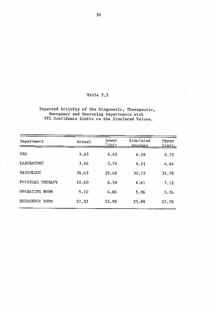
Table 3.3
Expected Activity of the Diagnostic, Therapeutic, Emergency and Operating Departments with
95% Confidence Limits on the Simulated Values.
Department Actual Lower Simulated Upper Limit Average Limit
EKG 9.63 6.43 6.59 6.75
LABORATORY 3.66 3.79 4,11 4.44
RADIOLOGY 34.43 29.68 30.73 31.78
PHYSICAL THERAPY 10.40 6.10 6.61 7.12
OPERATING ROOM 5.10 4,86 5.06 5.26
EMERGENCY ROOM 27.33 23.98 25.88 27.78
40
not unexpected for the specialized treatment areas, since available
data concerning them were minimal. In fact, the relatively good
values found for four of the six departments leads one to believe
that with sufficient information, the patient flow model would give
an excellent representation of the true system.
While actual new admissions were utilized to test the effective-
ness of the model, the number of carry-over patients who make up a
large portion of the inputs were generated by the model itself. Re-
call that the number of carry-over patients is found from the patient
flow model by using Equation 2.8. The elements of the carry-over row
of matrix ptt) | which gives the probability that a patient who began
in sector j is carried over, are multiplied by the corresponding inputs
to the system for the day. As an example, suppose thirty patients
(new admissions plus carry-overs) had entered the second floor on the
specific day for which Table 3.2 applies. In order to find the number
of patients carried over to the next day, one would multiply 30 by
%12,1> or in this case:
191% 30 = .9292 x 30 = 27.9
Approximately 28 patients would remain in the ward at the end of the
day. The remaining 2 patients would be discharged. Using row 11
of Table 3.2 with admissions, would also yield the number discharged.
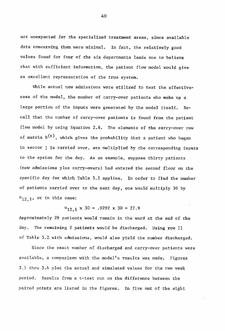
Since the exact number of discharged and carry-over patients were
available, a comparison with the model's results was made. Figures
3.1 thru 3.4 plot the actual and simulated values for the two week
period. Results from a t-test run on the difference between the
paired points are listed in the figures. In five out of the eight
Number
of
Patients
30
20
10
4l
Simulated
Actual
' Carry-over
/
A / ‘ !
\ / \,
A nA ey
e A
' \ Discharge f
ar / vi Lo y oan at
—__ ee , Ny
Day
= -.26 -2.16 < t.95< 2.16
~2.65 < t 9g < 2.65
ecarry-over
= 2.55 cdischarge
Figure 3.1
Simulated vs. Actual
Carry-over and Discharge for Medical/Surgical Floor 2
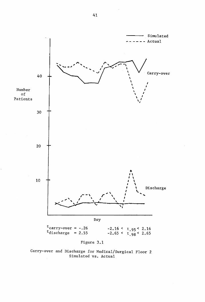
42
———— Simulated
meer ee Actual
Carry-over
40
Number
of
Patients \a
30 —
20
10 —p
Nn 7
ys / ‘ Ls Discharge Sy ee », —_ i AI
? \ 7 Av ‘ ‘
, ‘* ‘ / \ sO. }
Days
‘carry-over = -.76 ~-2.16< t.95< 2.16 tdischarge = -.60 -2.65< t9g< 2.65
Figure 3.2
Carry-over and Discharge for Medical/Surgical Floor 3
Simulated vs. Actual
43
Simulated
--- 4c Actual
20 =T
Number
of
Patients
10 =~
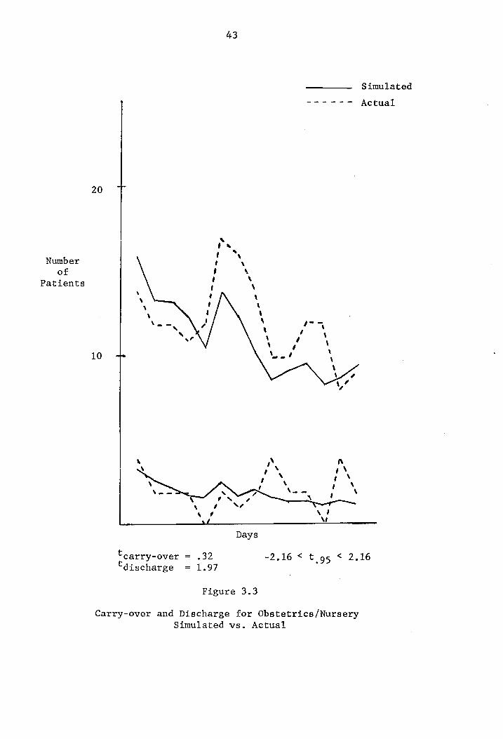
Days
ccarry-over = .32 -2.16 < t.g5 < 2.16 discharge = 1.97
Figure 3.3
Carry-over and Discharge for Obstetrics/Nursery Simulated vs. Actual
44
Simulated
wc ee ee Actual
20 TT
Number
of
Patients
Carry-over
10 7
Discharge
>> Aan o~.
7 ‘\ 7 v7 \,
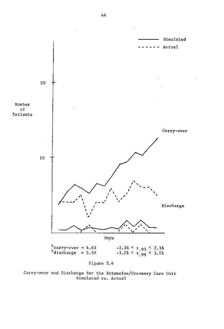
Days
ecarry-over = 6.63 -2.16 < t 95 < 2.16 discharge = 5.59 ~3.01 < t 99 < 3.01
Figure 3.4
Carry-over and Discharge for the Intensive/Coronary Care Unit Simulated vs. Actual
45
cases, the hypothesis that the simulated points are equivalent to the
true values could not be rejected under 95% confidence. For the number
of discharged patients on the second floor, the hypothesis would hold
using a 2% critical region. The actual discharge of 13 patients on the
eleventh day appears to be an unusual case, which incorporates a con-
siderable bias in the results. Neither the discharge nor carry-over
findings from the model were similar to the true values for the Intensive/
Coronary Care Unit. It appears that the model did not recover well from
a somewhat abnormal admission of six intensive care patients to the unit
on the sixth day. The problems arising from the unusual admissions or
departures to the system may be an indication that perhaps census as
well as care-level proportions should be taken into account in the re-
gression equations.
This section has given results from a patient flow model designed
for the Montgomery County Hospital. The model exhibited several de-
ficiencies, largely due to the lack of data needed to attain a represen-
tative system. While the results observed were far from perfect, an
illustration of the hospital model and the types of information that
it is capable of delivering has been effected. The next section makes
use of the model results for the allocation of nursing personnel.
The Staff Allocation Model
Information obtained from the patient flow model defined for the
two week period in the previous section was utilized in the formulation
of the nurse allocation model. Recall that care-level proportions are
46
needed in defining ward indices, w, 6t) , and the requirements estimates, i
R, 6), that are used in the staffing model described by Equation 2.16.
However, parts of the technical coefficient matrices of the patient flow
model were also dependent upon the care-level proportions. Therefore,
the care-level proportions are readily available for use in the staffing
model. In order to provide an example of how the care-level proportions,
ward indices and requirements are derived, a description of the basic
steps follows.
The first terms determined are the care-level proportions. The
care-level proportions are dependent upon the number of new admissions
and of the patients carried over from the previous day. Recall that
both the number of new admissions and carry-overs were separated into
care-levels. Suppose that the vector of admissions into ward 1 for a
specific day was
(yy, yy2"™, y93°) = (1, 2, 1),
and the vector of carry-overs into ward 1 from the previous day was
(04, ft), eyo 6th), c136F-))) = (4, 32, 3).
Using Equation 2.9, the proportion of self care patients would be:
(t) 14. 711°" = Gy3q = - 116
Similarly, 2496") and 24346) become .791 and .093, respectively. The
care-level proportions are found for each of the nursing wards. As
was stated in Chapter 2, the same care-level proportions are maintained
for the carry-overs of day t. For example, if of the 43 total patients
who entered sector 1 on day t, 40 are carried over, the new carry-over
vector would be:
47
(2) 50456) e546?) = 40 (24 (52,568) ,2, (ED) 9219 °° 2273
(4.64, 31.64,3.72)
(epg h% Cy 90 C73
The care-level proportions are now utilized in forming the re-
quirements terms, R, 64), The total expected number of patients en-
tering each ward, x; 6t), is also necessary. The assumption that care-
level proportions remain constant for the day is made again here for
each ward's expected treatment activity. The formulation of the nurs-
ing requirements used in this research is similar to the expressions
posed by Connor [10], Price [35], and Wolfe and Young [50]. The re-
quirements estimates are found from:
Ry 8) = (272415) + 532596 + 1372556" + 50)x, © /480
The value of R, 6t) is in terms of eight hour nurse days.
The ward importance indices also use the care-level proportions
for their definition. Using the proportion values from the example above
and Equation 2.14, the ward index for sector 1 would be:
w 6) = 241? + 2245‘) + 5213 = 2.163
With the requirement estimates and ward indices defined for each ward,
the constant terms needed for the objective function of Equation 2.16
are completed. Appendix C contains the care-level proportions, ward
indices and requirement estimates for the two week period under study.
Remaining to be defined are the constraints to the system. The
constraints are concerned with the staffing mix desired for the specific
wards as well as the specific numbers of the different skill classes
of nurses. The Montgomery County Hospital attempts to staff the same
number of nurses on each day. Thus, no distinction was made between
the days of the week for staffing purposes. The number of RNs, LPNs and
48
NAs used in the model were 18, 21 and 23, respectively.
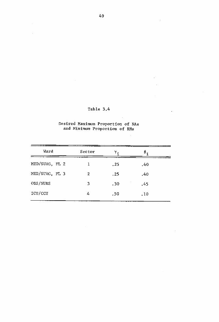
The staff mix constraints are concerned with a desired maximum per-
centage of nurses' aides, B,;, and a minimum proportion of registered
nurses, Y;, in a given ward. Table 3.4 shows the B; and y; values
utilized. Each ward has a desired mix dependent upon the types of pa-
tients treated in it. All of the necessary components are now defined
for the staff allocation model of Equation 2.16
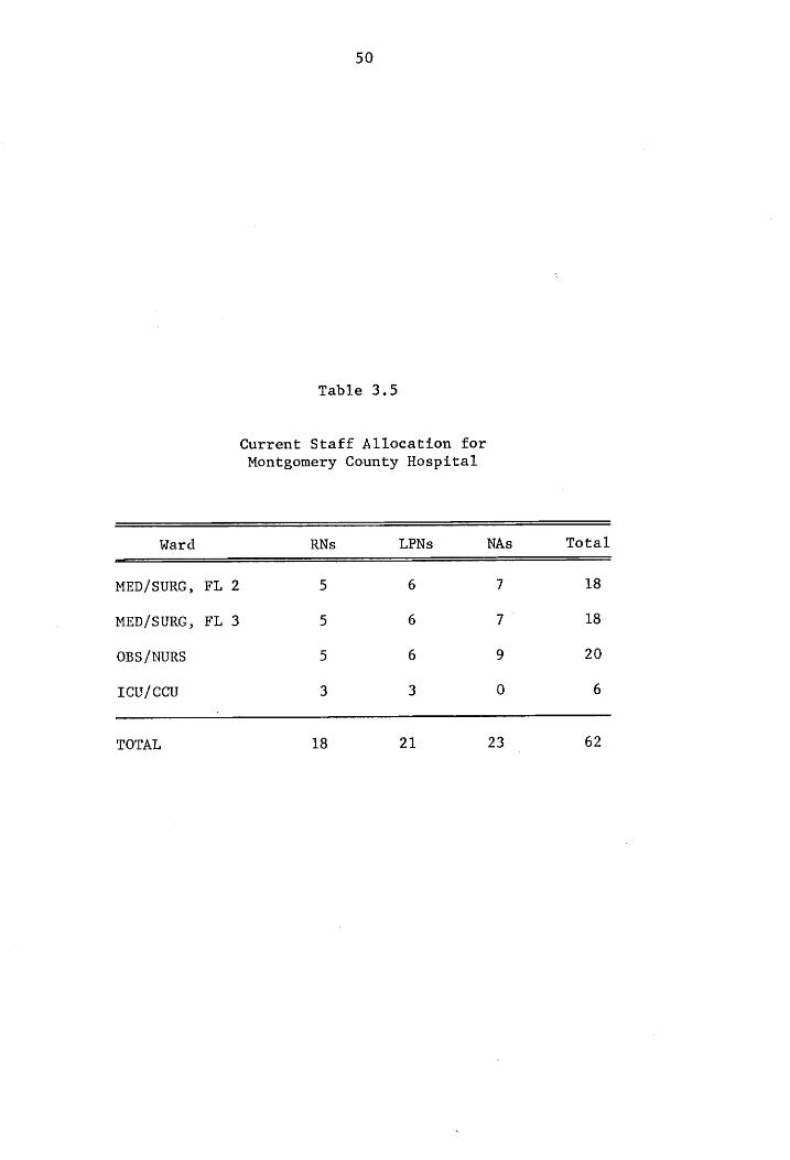
Before discussing the results found from the staffing model, the
current practices of staffing at the Montgomery County Hospital should
be noted. Table 3.5 shows the present staff allocation. As can be Seen,
the two medical/surgical wards have the same personnel distribution.
However, if one examines Appendix C, it is seen that the two wards do
not generally have the same requirements. In most cases, the nurse time
needs of the second floor exceed those of the third floor. The demand
for more nurse time on the second floor ranges from approximately one-
half to four nurse days. Also note that while the staff levels are con-
stant in the obstetrics and intensive care units, the number of maternity
and nursery patients is decreasing and the number of intensive care pa-
tients is increasing. While the actual nurse hours scheduled is more
than enough to satisfy the patient care demands in most cases, the in-
equities in the system are evident. Thus, the idea that sound quantitative
techniques could be valuable in improving personnel allocation is em-
phasized.
Solving the allocation problem using SUMT as described in Chapter 2,
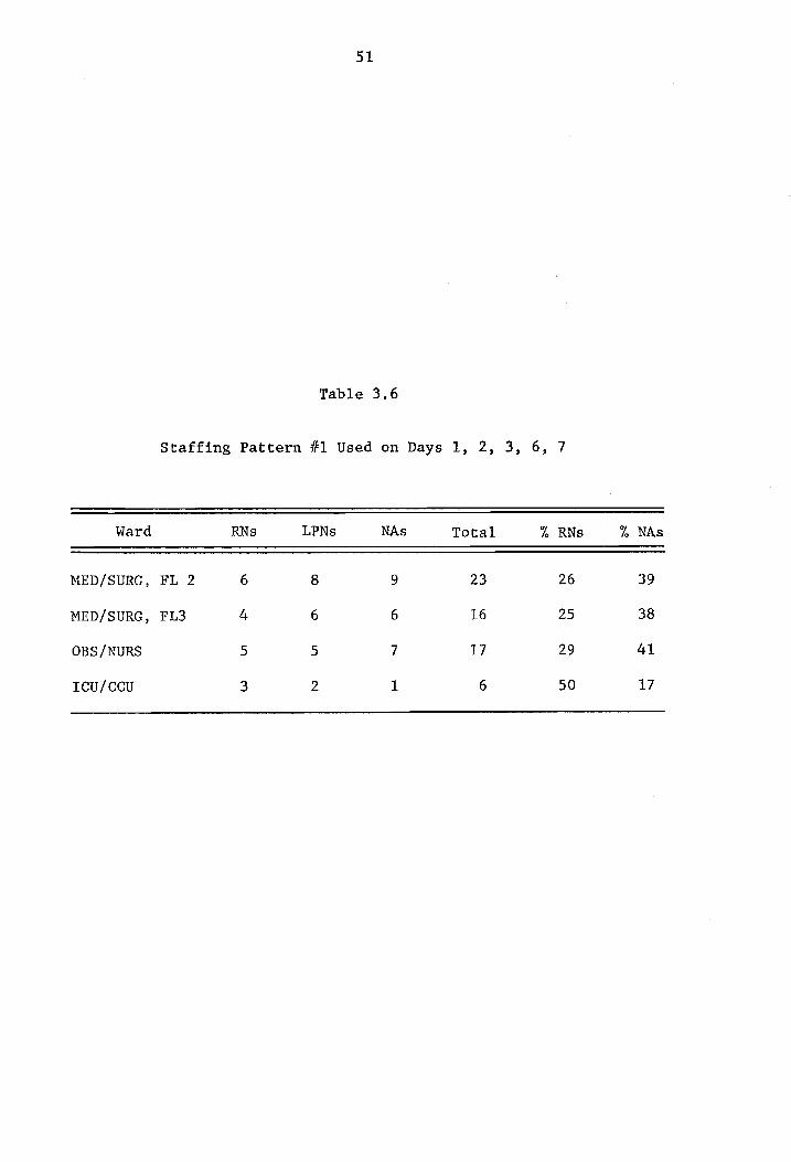
seven different staffing patterns were found for the two week period.
The staffing patterns are shown in Tables 3.6 thru 3.12. In all cases,
Desired Maximum Proportion of NAs and Minimum Proportion of RNs
49
Table 3.4
Ward Sector Ys By
MED/SURG, FL 2 1 25 40
MED/SURG, FL 3 2 .25 .40
OBS /NURS 3 .30 245
ICcu/CCcU 4 90 .10
50
Table 3.5
Current Staff Allocation for
Montgomery County Hospital
Ward RNs LPNs NAs Total
MED/SURG, FL 2 5 6 7 18
MED/SURG, FL 3 5 6 7 18
OBS /NURS 5 6 9 20
Icu/CCcU 3 3 0 6
TOTAL 18 21 23 62
51
Table 3.6
Staffing Pattern #1 Used on Days 1, 2, 3, 6, 7
Ward RNs LPNs NAs Total % RNs % NAs
MED/SURG, FL 2 6 8 9 23 26 39
MED/SURG, FL3 4 6 6 16 25 38
OBS/NURS 5 5 7 17 29 41
Icu/ccu 3 2 1 6 50 17

52
Table 3.7
Staffing Pattern #2 Used on Days 5, 9
Ward RNs LPNs NAs Total % RNs % NAs
MED/SURG, FL 2 4 7 8 19 21 42
MED/SURG, FL 3 4 7 8 19 21 42
OBS /NURS 4 4 7 15 27 47
ICU/CCU 6 3 0 9 67 0
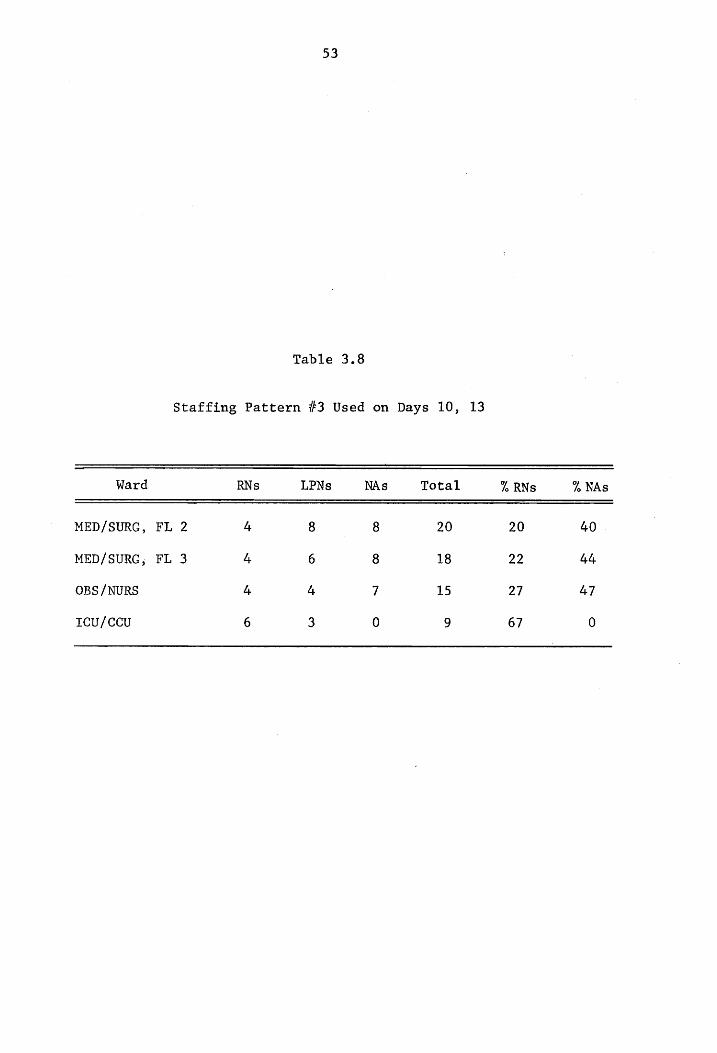
Staffing Pattern #3 Used on Days 10, 13
53
Table 3.8
Ward RNs LPNs NAs Total % RNs 7, NAS
MED/SURG, FL 2 4 8 8 20 20 40
MED/SURG, FL 3 4 6 8 18 22 44
OBS /NURS 4 4 7 15 27 47
TCU/CCU 6 3 0 9 67 0
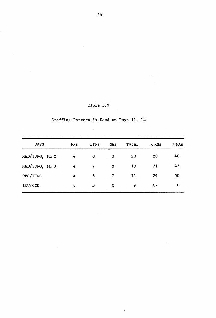
Staffing Pattern #4 Used on Days 11, 12
54
Table 3.9
Ward RNs LPNs NAs Total % RNs % NAs
MED/SURG, FL 2 4 8 8 20 20 40
MED/SURG, FL 3 4 7 8 19 21 42
OBS /NURS 4 3 7 14 29 50
Icu/Ccu 6 3 0 9 67 0
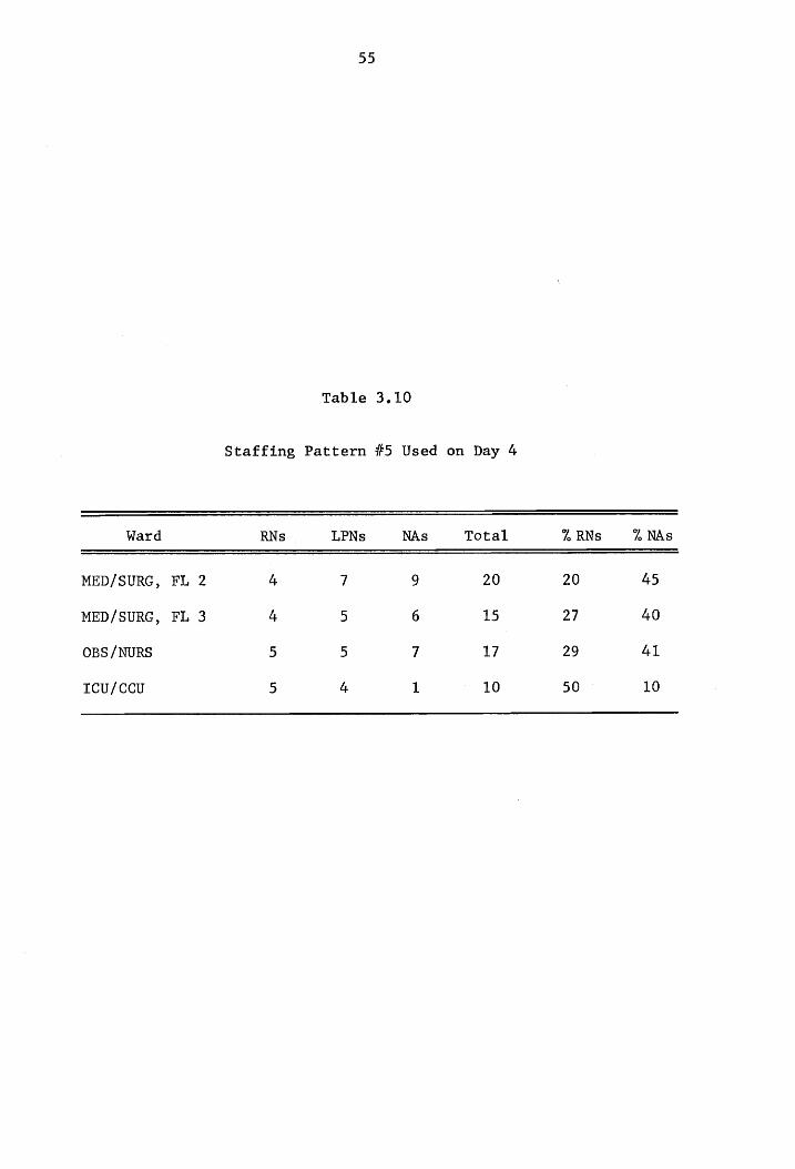
55
Table 3.10
Staffing Pattern #5 Used on Day 4
Ward RNs LPNs NAs Total % RNs % NAs
MED/SURG, FL 2 4 7 9 20 20 45
MED/SURG, FL 3 4 5 6 15 27 40
OBS/NURS 5 5 7 17 29 41
ICU/CCU 5 4 1l 10 50 10
56
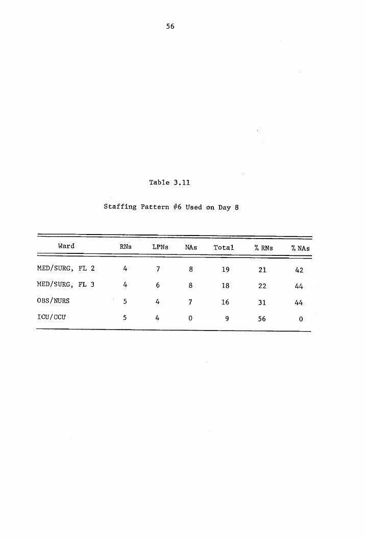
Table 3.11
Staffing Pattern #6 Used on Day 8
Ward RNs LPNs NAs Total % RNs % NAs
MED/SURG, FL 2 4 7 8 19 21 42
MED/SURG, FL 3 4 6 8 18 22 44
OBS/NURS 5 4 7 16 31 44
Lcu/ccu 5 4 0 9 56 0

57
Table 3.12
Staffing Pattern #7 Used on Day 14
Ward RNs LPNs NAs Total % RNs % NAs
MED/SURG, FL 2 4 7 8 19 21 42
MED/SURG, FL 3 3 6 6 15 20 40
OBS /NURS 5 4 8 17 29 47
Icu/Ccu 6 4 1 11 55 9
58
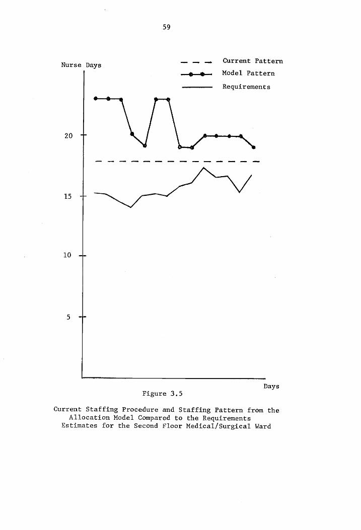
the equality constraints were satisfied. While the minimum and maximum
percentage of RNs and NAs were not always met, each solution did re-
main fairly close to the desired mix. In order to illustrate the dif-
ferences between the current staffing practices at the Montgomery County
Hospital and the staffing model results, graphical representations of
the two patterns along with the requirements estimates are shown in
Figures 3.5 thru 3.8.
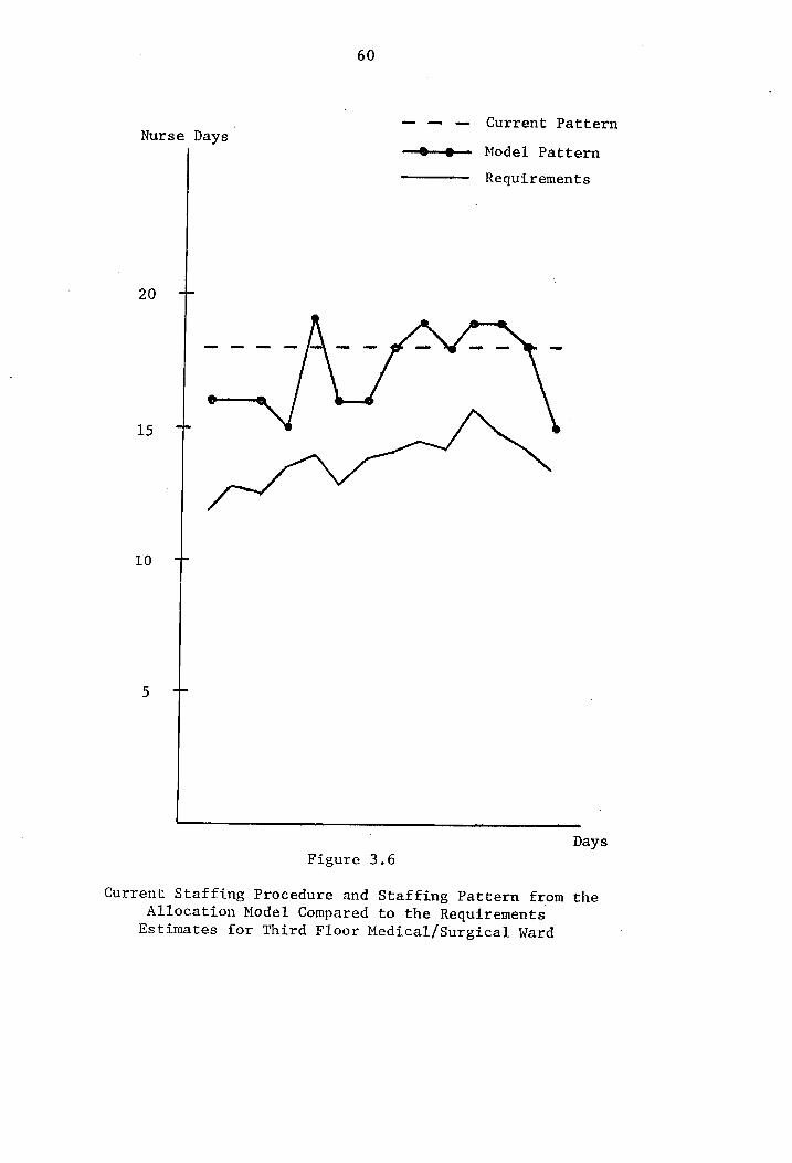
The graphs give an indication of the staffing model's dependence
on the requirements estimates. The importance of the ward indices and
staff mix constraints is also evidenced by the graphs. Without the ward
indices acting as weights in the objective function, one would expect
the differences between the staff allocation and the requirements es-
timates to be approximately the same for each ward on any day. Using
the weighted system, however, the wards with the larger ward indices are
allowed a larger difference between the staff allocation and the require-
ments estimates, if overstaffing is the case. Thus, the obstetrics
ward exhibits a greater separation between the staff allocation and
requirements estimates than the differences for the two medical/surgical
wards. Since the intensive/coronary care unit has the highest ward
index, the staffing model should allow it the greatest difference be-
tween the staff allocation and requirements estimate. To explain the
reason for the intensive/coronary care unit having smaller differences
between the allocation of the nursing staff and estimated requirements
than the obstetrics ward, it is necessary to consider the system con-
straints. For the intensive/coronary care unit, at least half of the
staff is desired to be RNs. Therefore, additions to the unit's staff
59
— — ow Current Pattern Nurse Days
—e—o—~ Model Pattern
Requirements
20 7
I +
10 =
5 +
Days Figure 3.5
Current Staffing Procedure and Staffing Pattern from the Allocation Model Compared to the Requirements
Estimates for the Second Floor Medical/Surgical Ward
60
— — — Current Pattern Nurse Days
—®—e@— Model Pattern
Requirements
20 7
10 —
Days
Figure 3.6
Current Staffing Procedure and Staffing Pattern from the Allocation Model Compared to the Requirements
Estimates for Third Floor Medical/Surgical Ward
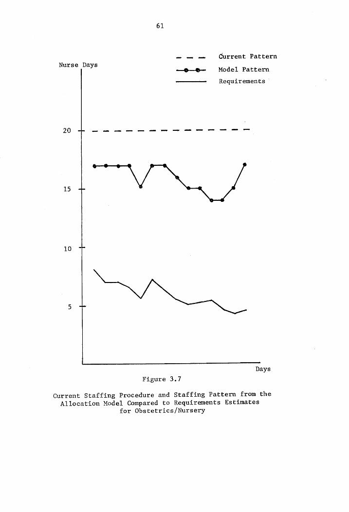
61
- — — Current Pattern
Nurse Days —o—O— Model Pattern
—_—_——— Requirements ©
DO meee cee eee ee
15 +
10 +
5 —- Days
Figure 3.7
Current Staffing Procedure and Staffing Pattern from the
Allocation Model Compared to Requirements Estimates
for Obstetrics/Nursery
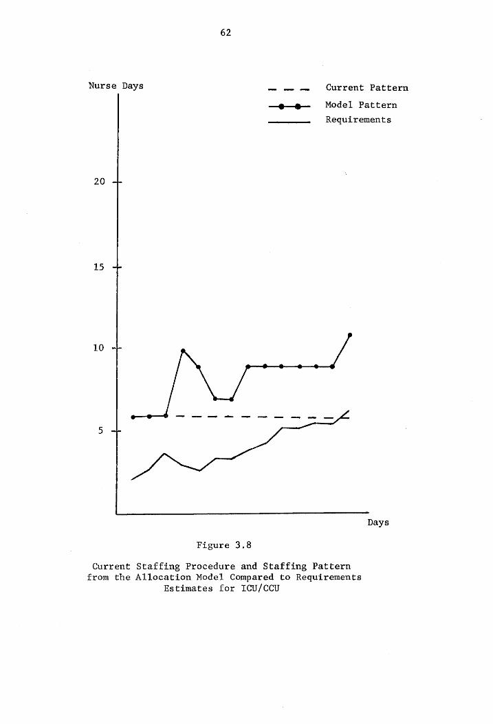
62
Nurse Days — — — Current Pattern
—@e—@— Model Pattern
Requirements
20 -+-
15 --
10 --
5 4.
Days
Figure 3.8
Current Staffing Procedure and Staffing Pattern from the Allocation Model Compared to Requirements
Estimates for ICU/CCU
63
would be RNs in most cases. However, only a limited number of RNs are
available and several must be allocated to each ward. Thus, the staff
mix constraint for the intensive care ward prohibits a greater difference
between the staff allocation and requirements estimate.
The results presented thus far have been concerned with a specific
study period for which actual admissions data were used. However, if
personnel allocation is to be performed in advance, perfect information
concerning admissions will rarely be available. Therefore, it is im-
portant to realize how sensitive the staffing allocation model is to
errors in the admissions data. The following section discusses the
sensitivity of the staffing model to variations in the admissions data.
Sensitivity of the Staff Allocation Model
Assuming the hospital patient flow model yields an acceptable
representation of the hospital system, it is of interest to know how
sensitive the staff allocation model is to any errors that occur in
the admission inputs. Knowledge of the model's sensitivity will indi-
cate the precision needed in forecasting the number of unsecheduled
admissions (or total admissions if long range planning is desired).
To test the model's sensitivity under different admissions con-
ditions, simulated values were used. The actual admissions data for
each care-level and ward were compared to corresponding Poisson dis-
tributions using a Kolmogorov-Smirnov goodness-of-fit test. Results
of the test are found in Appendix D. Using the parameters shown in the
appendix, two weeks of admission data were generated and used in the
patient flow model. Thus, a normal period was obtained for comparative
64
purposes. Nine different staffing patterns were found for the normal
period.
In order to check the sensitivity of the model to large errors in
the number of admissions predicted, the parameters for the admission
distributions were increased and decreased by 20%. With the predicted
number of patients increased, less than 15% of the patterns obtained
corresponded to the staff allocations for the normal period. Less than
22% of the patterns obtained for the decreased admissions case matched
those of the normal period. The effects of an increase in the number
of admissions of a specific care-level classification were also examined.
When the number of admissions of a particular care-level were increased,
the new patterns obtained coincided with those of the normal period less
than 30% of the time. A total of 27 different staffing arrangements
were examined. The allocation model, therefore, appears to be sensitive
to any large errors in admissions.
Next, sensitivity of the allocation model to small changes in
admissions was tested. Results from one particular day of the study
period were chosen for a standard of comparison. The number of admis-
sions by care-level and ward were then allowed to vary between plus and
minus one of the original admissions set in a random fashion. Random
numbers were used for deciding whether the number of admissions in a
specific category should be increased by one, decreased by one, or
remain the same. Nine digit random numbers were used with one digit
corresponding to each possible admission category, for example, self
care admissions to the medical/surgical ward on the second floor. If
the random digits were 1, 2 or 3, the number of admissions for that
65
category were decreased by one. The occurrence of random digits 4, 5
or 6 caused the number of admissions to increase by one. When the
remaining digits occurred no changes were made in the number of ad-
missions to the particular category. Thus, there was a 60% chance
that the number of admissions of a particular care-level to a specific
ward would be changed by one. Appropriate changes were made to the
ward indices and requirements estimates since they are dependent upon
the number of admissions. One hundred trials were run. The staffing
pattern for the day changed 65% of the time. Thus, results from the
staffing allocation model appear sensitive to errors in the number of
patient admissions.
The reaction of the staffing model to changes in the number of
available nurses was also examined. Results with decreases in the
number of RNs, LPNs, NAs and different combinations of the nursing
types were observed. In most cases, considerable changes in the staff
allocation were obtained. In other words, if one less registered nurse
was available on a specific day, the only change in the staff allocation
would not be a decrease of one registered nurse in a particular ward.
Realignment of all three types of nurses usually resulted. The large
shifts in the personnel realignment were due mainly to the allocation
model's attempt to satisfy the staffing mix constraints in the best
possible manner. As a result, it is not possible to predict the re-
action of the staffing model to a change in the number of personnel
available in any simple manner.
66
Use of the Staffing Model
Thus far, this chapter has illustrated the use of a hospital
patient flow model for predicting patient demands in different hos-
pital sectors and the use of a staff allocation model derived from
it. However, the staffing model was also shown to be sensitive to
any small errors that might occur in predicting the number of admis-
sions. Because of the staffing model's sensitivity, its usage for
preparing schedules far in advance does not seem practical. However,
the staffing model can be useful along with the concept of controlled
variable staffing.
Controlled variable staffing involves the maintenance of a base,
or fixed, staff on each ward and a pool of nurses who "float" from
one ward to another, depending on daily needs. As stated by Wolfe
and Young [50], the procedure receives its name because
"6. 6. 6 the total staff on each nursing unit is variable,
according to needs, but control is maintained over the
amount of supplementary staff assigned to each unit."
The staffing model can be used for making decisions concerning a base
staff. From the results of the staffing model for a given study,
the minimum number of nurses of each type found in a ward on any day
would be the number of nurses assigned to the base staff. The remain-
ing nurses would be placed in the float pool, Table 3.13 shows the
base and float staffing arrangement for the two week period studied.
The staffing model could be used to set up the base and float staff
assignments on a seasonal or monthly basis, or when a turnover in
personnel warrants adjustments.
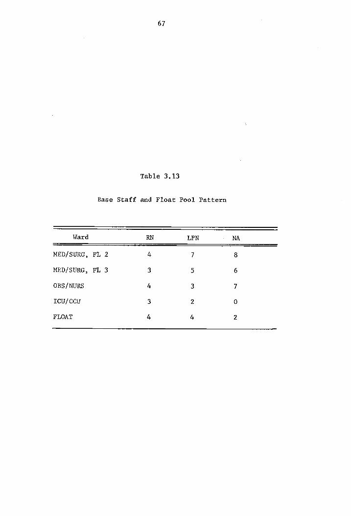
67
Table 3.13
Base Staff and Float Pool Pattern
Ward RN LPN NA
MED/SURG, FL 2 4 7 8
MED/SURG, FL 3 3 5 6
OBS/NURS 4 3 7
rcu/ccu 3 2 0
FLOAT 4 4 2
68
While the staffing model is useful in assigning a base staff,
the nurses in the float pool must be assigned on a daily basis. A
simple procedure for aiding in the placement of personnel from the
float pool will now be described,
The ward indices can be utilized for the assignment of the float
pool nurses. Preparation of the schedule for the float pool nurses
should be performed at some specific time on the previous day, mid-
night, for example. At that time, the number of patients by care-
level in each ward can be used to define ward indices. A new index
called a float pool proportion, FPP, , can be derived for each ward
using Equation 3.1:
wy °Py FPP = ———
Swe Ps qi *i
where
FPP; = the proportion of the float pool staff to be assigned
to ward i. ‘
w; = the ward index at the schedule preparation time.
P; = the patient census at the schedule preparation time.
By multiplying the number of nurses in the float pool by the
float pool proportion for each ward, a guideline for the staff as-
signment is obtained. The float pool proportion can also be used to
aid in deciding the nursing levels assigned to each ward.
As an illustration of the above procedure, suppose that at
midnight on a specific day the ward census was that of Table 3.14,
The ward indices are also show in the table. The float pool staff
is that of Table 3.13. The float pool proportion for ward 1 is then
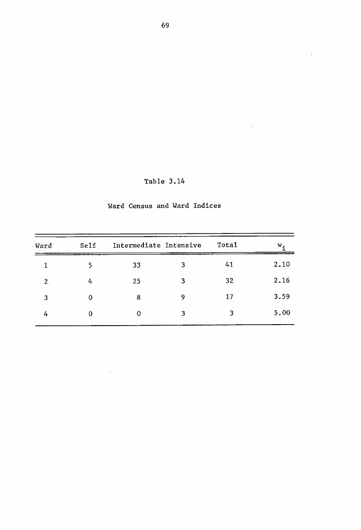
69
Table 3.14
Ward Census and Ward Indices
Ward Self Intermediate Intensive Total Ws
1 5 33 3 Al 2.10
2 4 25 3 32 2.16
3 0 8 9 17 3.59
4 0 0 3 3 5.00
70
then calculated as follows:
FPP, = fa." 5 5 5 = +29 41(2.1)° + 32(2.16)* + 17(3.59)* + 3(5)
The float pool proportions for wards 2, 3 and 4 are .24, .35 and
.12, respectively. Multiplying the proportions by the number of
nurses in the float pool and rounding to the nearest integer, the
wards would receive 3, 2, 4 and 1 additional nurses. To keep some
balance in the staffing, the order of assigning the personnel could
be done by nursing level or some ranking method for each of the float
pool nurses, depending on training, experience, seniority or some other
system. Any available information concerning the patient admissions
and discharges for the next day should also be included when pre-
paring the schedule for the float pool nurses.
Thus, the concept of controlled variable staffing can be used
with the staff allocation model forming the base staff. However, if
the percentage of unscheduled patients entering the hospital is very
small and the number of scheduled patients is known in advance, the
staffing model alone can be used on a short term basis for assigning
nursing personnel. It should also be noted that the results from the
model were concerned with assigning the staff for the entire day. In
some cases, dividing the entire day's staff into thirds for each shift
would be suitable. For other cases, it may be advisable to solve a
system similar to Equation 2.16, with constraints and requirements
estimates formulated for each shift in the study period.
71
Cost Model Results
In Chapter 2, several results for absorbing Markov chains were
described that can be useful for finding several cost related es-
timates from the patient flow model. This section provides an il-
lustration of typical results obtained from the cost model. The
results for this section were derived from the technical coefficient
matrices describing the patient transfer behavior in the Montgomery
County Hospital for a two week period.
The only new information needed to apply the cost model results
of Chapter 2 is a diagonal matrix containing the costs incurred by
a patient in a given sector of the hospital. Using Equations 2.18
thru 2.21, estimates of expected revenue and the variance of the reve-
nue were obtained. Table 3.15 shows several revenue related results
for a typical day. Also shown in the table are the service charges
used in the study. Room rates were not included in the service charges
because patients returning to the ward from some specialty unit would
have been charged two or more times for the room fee.
The figures under the expected revenue column of Table 3.15 give
the expected revenue generated before absorption by a patient who
began in the particular sector. For example, a patient who begins
in the medical/surgical ward on the second floor is expected to in-
cur charges of $6.26 for special hospital services. The large values
for the variance of revenue are due to the fact that a large percen-
tage of the patients go to an absorption state in one step. However,
a very small number of patients reach the absorption states in two
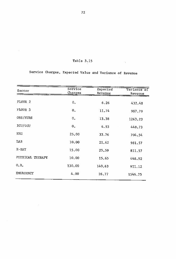
72
Table 3.15
Service Charges, Expected Value and Variance of Revenue
Service Expected Variance of Sector Charges Revenue Revenue
FLOOR 2 0, 6.26 432.48
FLOOR 3 0. 11.74 987.79
OBS /NURS 0, 13.38 1263.23
Icu/ccu 0, 6.53 448.73
EKG 25.00 33.76 704.54
LAB 10.00 21.62 981.57
X-RAY 15.00 25.59 811.57
PHYSICAL THERAPY 10.00 15.65 448.92
O.R. 130.00 140.63 911.12
EMERGENCY 4,00 26.77 1546.75
73
steps, since in the formulation of the patient flow model patients
could not be discharged or carried over from many of the special
services sectors. Thus, if a patient does not go directly to an ab-
sorption state, he is likely to take three or four steps before
reaching the departure or carry-over state, hence, increasing his
charges. Therefore, the differences from mean values tend to be
large, and since the variance involves squared terms, it tends to be
large.
In order to obtain the total expected revenue generated in the
hospital, the expected revenue figures of Table 3.15 were multiplied
by the number of patients entering each sector (both new admissions
and carry-overs). Room charges were added to the model by multiplying
the number of carry-over patients in each sector by the appropriate
room rates. Table 3.16 gives the total expected revenue from the
different wards for a particular day.
The cost model can be used to compare expected revenue to ex-
penditures, to test changes in service charges or to find the rela-
tionships between revenue and various hospital departments or census.
Figure 3.9 shows the relationship between revenue and total hospital
census. The relationship found using linear regression can be stated as:
Revenue = 1298 + 35.6 (census) (3.2)
When the census was broken down by the number of patients in each care-
level, the following similar relationship was found:
Revenue = 1282 + 36.05 Py + 35.46 Py + 36.62 Py (3.3)
where
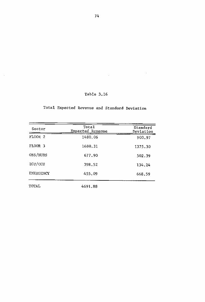
74
Table 3.16
Total Expected Revenue and Standard Deviation
Sect Total Standard ector Expected Revenue Deviation
FLOOR 2 1480.06 900.97
FLOOR 3 1680.31 1375.30
OBS /NURS 677.90 502.39
Icu/CCcu 398.52 134.24
EMERGENCY 455.09 668.59
TOTAL 4691.88
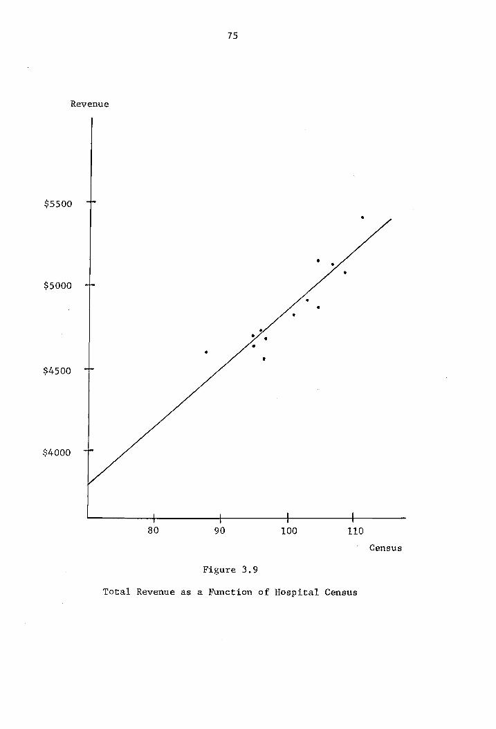
75
Revenue
$5500
$5000
$4500
$4000 | | { | | I I 1
80 90 100 110
Census
Figure 3.9
Total Revenue as a Function of Hospital Census
76
P, = the total number of hospital patients in care-level k.
Functions of the above type can be used periodically in conjunction
with census forecasts as an aid in preparing the budget.
For the cost model to be utilized a matrix of service charges
is needed. While some services may have fixed charges, others may
have variable charges depending upon a patient's specific condition.
For example, a glucose tolerance test and a brain scan are both lab-
oratory functions but involve different charges. The charges used
in the cost model must, therefore, be some average cost for the ser-
vice. If the distribution of the charges is known, however, a
method called Graphical Evaluation and Review Technique (GERT) [36] [37]
[48] can be used with the transfer probabilities from the technical
coefficient matrices. The GERT method makes use of the moment gen-
erating function of the cost distribution in arriving at similar re-
sults to the cost model presented in this section.
summary
This chapter has provided results obtained from use of the
models described in Chapter 2. A patient flow model was derived from
data obtained from the Montgomery County Hospital. Results concerning
patient demands on different hospital departments and the number of
discharged and carry-over patients were compared to the Montgomery
County Hospital's actual demands for a two week study period. Making
use of the care-level proportions and patient demands upon the wards
from the patient flow model results, the staff allocation model was
utilized. The staffing patterns were found to be sensitive to errors

77
in the number of new admissions. Because of the sensitivity of the
staffing model, the concept of controlled variable staffing was pre-
sented. A simple procedure for the assignment of the float pool
nurses was also discussed, Finally, typical results from the use of
the cost model were presented.
Chapter 4
SUMMARY AND RECOMMENDATIONS FOR FURTHER RESEARCH
Summary
The objective of this research was to illustrate the applicability
of a hospital patient flow model in addressing hospital resource alloca-
tion problems. In particular, a model for allocating ward nurses was
designed from information provided by the hospital patient flow model.
A method for obtaining hospital revenue estimates was also presented.
A survey of the literature reveals numerous forecasting models for
hospital application and several methods for the allocation of nursing
personnel. A need to connect an allocation model to a forecasting model
was indicated. Most of the forecasting models were concerned with pre-
dicting patient census or bed utilization. The nurse staffing methods
generally were concerned with minimizing some shortage cost for not
meeting patient demands. The staffing literature indicated that patient
demand predictions should be based on patient care-levels. In this
thesis, a staffing model was developed from the specific information pro-
vided by a hospital patient flow model which takes patient care-levels
into account. The staffing model considers more than the minimization
of some shortage cost since the literature review indicates that over-
staffing in hospital wards is a common occurrence.
Three separate but interrelated models were presented in this
78
79
thesis, First, a hospital patient flow model was discussed. An
existing hospital patient flow model was used in this research. The
main feature of the hospital patient flow model is the matrix of tech-
nical coefficients. The technical coefficient matrix gives the pro-
bability of a patient transferring from one sector of the hospital to
another, Elements of the technical coefficient matrix are based on
the proportion of patients in each care-level in a ward. The formula-
tion of the technical coefficient matrix is recognized as an absorbing
Markov chain and several results for absorbing Markov chains are used
to obtain patient demands upon the different hospital services given
the system's daily patient input.
From the results of the patient flow model concerning the ward
demands, a staff allocation model was developed. The objective of the
staffing model is the minimization of a weighted quadratic penalty
function. The penalty values are dependent upon the magnitude of the
difference from the requirements predicted from the hospital patient
flow model and a weighting factor. The weighting factor depends on a
ward importance index and whether overstaffing or understaffing in the
ward is the case. The ward importance index is rating of each ward
depending on its care-level proportions. Constraints to the model are
the number of nurses available and a desired mix of RNs, LPNs and NAs
for each ward. Solution of the allocation model in this thesis was
obtained by using SUMT with a pattern search.
Finally, a model concerned with predicting hospital revenues
was presented. Again, results for absorbing Markov chains were utilized
with the technical coefficient matrix to provide estimates of the ex-
80
pected value and variance of a hospital's revenue.
In order to illustrate the use of the models, results from a two-
week study period of the Montgomery County Hospital were presented and
discussed. The staff allocation model was found to be sensitive to errors
in predicting the number of new admissions. As a result, a description
of a method for controlled variable staffing was provided. As an ex-
ample of the cost model's use, the relationship between hospital revenue
and census was presented.
In summary, several quantitative techniques for hospital ap-
plications have been presented. The general effectiveness of the hos-
pital patient flow, staff allocation and cost models was shown through
the results of a two-week study period for an actual hospital.
Recommendations for Further Study
Several areas for the extension of this research have been recog-
nized and are listed below:
1) Consider further testing concerning the formulation of the
technical coefficients matrix. Factors other than care-
level proportions may affect a patient's transfer behavior.
For example, the total hospital census might influence
the probabilities of a patient's transfer.
2) Consider dividing wards into care-level sectors. For ex-
ample, a medical/surgical ward would be divided into three
sectors, one for each care-level classification. Such a
division would provide further insight into the depend-
ence of patient transfer behavior to patient care-level.
3)
4)
5)
6)
81
An indication of how a patient's care-level changes over time
could also be a derivative of the care-level divisions.
Consider the development of a new billing structure in which
a patient incurs charges in the ward according to his
care-level. Adapting the patient flow model as in the
recommendation above would probably simplify examining
a care-level based billing system. A care-level based
billing system would provide a more equitable system of pay-
ment for patients in the same ward who do not necessarily
require the same nursing attention.
Consider obtaining the cost distributions and their rela-
tionship to patient care-levels for use in a cost model,
A method such as GERT could be used with the distributions to
obtain more specific hospital revenue estimates.
Consider introducing costs for the different types of nurses
into the staff allocation model to obtain an optimal level
and mix for the hospital's nursing staff.
Consider using information from the hospital patient flow ~
model concerning the frequency of transfers between the
different hospital sectors to design the layout of the
hospital facilities.
10,
11.
12,
13.
BIBLIOGRAPHY
Abernathy, W. J., Nicholas Baloff, and John C. Hershey, ''The Nurse
Staffing Problem: Issues and Prospects,"' Sloan Management
Review, Vol. 12, Fall 1971.
American Hospital Association and National League of Nursing
Education, Hospital Nursing Service Manual, National League
for Nursing, New York, 1950.
Balintfy, Joseph L., "A Hospital Census Predictor Model," in
Hospital Industrial Engineering, Smalley and Freeman (eds.),
Reinhold Publishing Corp., New York, 1966.
Barnoon, Shlomo, and Harvey Wolfe, "Scheduling a Multiple Operating
Room System: A Simulation Approach,"' Health Services Research,
Winter 1968. |
Barr, Alex, 'Measuring Nursing Care," Problems and Progress in
Medical Care, Oxford University Press, New York, 1964.
Beenhakker, Henri L., "Multiple Correlation - A Technique for
Prediction of Future Hospital Bed Needs,"' Operations Research,
Vol. 11, No. 8, 1963.
Blumberg, Mark S., "DPF Concept Helps Predict Bed Needs,"' Modern
Hospital, Vol. 97, December 1961.
Cohen, David M., A Hospital Patient Care Flow Model of Stochastic
Structure, Ph.D. Dissertation for Pennsylvania State
University, 1972.
Connor, R. J., “Hospital Work Sampling with Associated Measures
of Production," Journal of Industrial Engineering, Vol. 12,
March-April 1961.
Connor, R. J., "A Work Sampling Study of Variations in Nursing
Work Load," Hospitals, Vol. 35, No. 9, May 1, 1961.
Connor, R. J., C. D. Flagle, R. K. C. Hsieh, R. A. Preston, and
S. Singer, "Effective Use of Nursing Resources: A Research
Report,'’ Hospitals, Vol. 35, No. 9, May 1, 1961,
Connors, Michael M., "A Stochastic Elective Admissions Scheduling
Algorithm," Health Services Research, Winter 1970.
Dantzig, George B., "Optimal Solution of a Dynamic Leontief Model
with Substitution," Econometrica, Vol. 23, No. 3, July 1955.
82
14.
15.
16.
17.
18.
19,
20.
21.
22.
23.
24.
25.
26.
27.
28.
83
Derman, Cyrus, 'On Sequential Decisions and Markov Chains,"
Management Science, Vol. 9, No. 1, 1962.
Feldstein, Martin S., The Rising Cost of Hospital Care, Information
Resources Press, Washington, D. C., 1971.
Fetter, Robert B., and John D. Thompson, "The Simulation of
Hospital Systems,"' Operations Research, Vol. 13, No. 5,
September-October 1965.
Feyerherm, A. M., "Nursing Activity Patterns: A Guide to Staffing,'' Nursing Research, Vol. 15, Spring 1966.
Fiacco, Anthony V., and Garth P. McCormick, Nonlinear Programming;
Sequential Unconstrained Minimization Techniques, John
Wiley and Sons, Inc., New York, 1968.
Flagle, Charles D., "Operations Research in a Hospital," in Operations Research and Systems Engineering, Flagle, C. D.,
W. H. Higgins, and R. H. Roy (eds.), John Hopkins Press, Baltimore, Maryland, 1960.
Griffith, John R., Quantitative Techniques for Hospital Planning
and Control, D. C. Heath and Co., Lexington, Massachusetts,
1972,
Harris, David H., "Nursing/Staffing Requirements," Hospitals,
Vol. 44, April 16, 1970.
Holbrook, Fred K., "Charging by Level of Nursing Care," Hospitals, Vol. 46, No. 16, August 16, 1972.
Howard, Ronald A., Dynamic Programming and Markov Processes,
The M. I. T. Press, Cambridge, Massachusetts, 1966.
Jackson, John E., An Analysis of the Bed Allocation Problem,
Master's thesis for Virginia Polytechnic Institute and State University, September 1971.
Jelinek, Richard C., Tim K. Zin, G. L. Delon, and Ralph A. Aleman,
"A Nursing Scheduling and Allocation System in Operation,"
ATIE, Technical Papers 1972.
Kemeny, J. G., and J. L. Snell, Finite Markov Chains, D. Van
Nostrand, Inc., Princeton, New Jersey, 1960.
Kolesar, Peter, "A Markovian Model for Hospital Admission
Scheduling,'' Management Science, Vol. 16, No. 6, February 1970.
Leontief, Wassily W., Input-Output Economics, Oxford University
Press, New York, 1966,
29.
30.
31.
32.
33.
34.
35.
36.
37.
38.
39.
40.
41,
84
Luck, G. M., J. Luckman, B. W. Smith and J. Stringer, Patients,
Hospitals and Operational Research, Travistock Publications,
London, 1971.
McConnell, Campbell R., McConnell Economics, McGraw-Hill Book
Company, New York, 1969.
Miernyk, William H., The Elements of Input-Output Analysis,
Random House, Inc., New York, 1965.
Olson, Charles H., “Projecting Manpower Requirements from Staffing Utilization Charts," AITE, Technical Papers 1972.
Packer, A. H., "Applying Cost-Effectiveness Concepts to the Community Health System," Operations Research, Vol. 16, 1968
Preston, Ruth A., Kerr L. White, E. Josephine Strachan, and H.
Bradley Wells, "Patient Care Classification as a Basis for Estimating Graded Inpatient Hospital Facilities," Journal of
Chronic Diseases, Vol. 17, No. 9, 1964.
Price, Elmina M., Staffing for Patient Care, Springer Publishing
Company, Inc., New York, 1970.
Pritsker, A. A. B., and W. W. Happ, "GERT: Graphical Evaluation
and Review Technique, Part I, Fundamentals," Journal of
Industrial Engineering, Vol. 17, No. 5, May 1966.
Pritsker, A. A. B., and G. E. Whitehouse, "GERT: Graphical
Evaluation and Review Technique, Part II, Probabilistic and Industrial Engineering Applications," Journal of Industrial Engineering, Vol. 17, No. 6, June 1966.
Purcell, John R., An Investigation of Self-Adaptive Forecasting
Models for Predicting Health Service Demands, Master's
thesis for Virginia Polytechnic Institute and State
University, November 1972.
Robinson, Gordon H., Paul Wing, and Louis E. Davis, "Computer
Simulation of Hospital Patient Scheduling Systems," Health Services Research, Summer 1968.
Ryan, Joseph R., and Gordon D. Boydston, "This Flexible Staffing Plan Puts Nurses in Right Place at Right Time," Modern
Hospital, Vol. 105, No. 3, September 1965.
Shonick, William, "Understanding the Nature of the Random
Fluctuations of the Hospital Census,'' Medical Care, Vol.
10, No, 2, March-April 1972.
42,
43,
Ah,
45,
46,
47.
48,
49.
50.
51.
52,
85
Soriano, A., A Comparative Study of Block and Individual Appoint- ment Systems in the Outpatient Department: Wilmer Ophthalmo- logical Clinic, Progress Report, USPHS Grant W-167.
Thierauf, Robert J., and Richard A. Grosse, Decision Making Through Operations Research, John Wiley and Sons, Inc., New York, 1970.
Thompson, John B., Oscar Wade Avant, and Ellwayne D. Spiker, “How Queuing Theory Works for the Hospital," Modern Hospital, Vol. 94, No. 3, March 1960.
Wagner, Harvey M., "A Linear Programming Solution to Dynamic Leontief Type Models," Management Science, Vol. 3, No. 3, 1957,
Warner, D. M., and Juan Prawda, "A Mathematical Programming Model for Scheduling Nursing Personnel in a Hospital," Management Science, Vol. 19, No. 4, December 1972.
White, John A., "On Absorbing Markov Chains and Optimum Batch Production Quantities," AILE Transactions, Vol. 11, No. 1, March 1970.
Whitehouse, G. E., and A. A. B. Pritsker, "GERT: Graphical Evaluation and Review Technique, Part III, Further Statistical Results: Counters, Renewal Times, and Correlations," AIIE Transactions, Vol. 1, No. 1, March 1969.
Wilde, Douglass J., and Charles S. Beightler, Foundations of Optimization, Prentice~Hall, Inc., Englewood Cliffs, New Jersey, 1967.
Wolfe, Harvey, and John P. Young, "Staffing the Nursing Unit,"
Nursing Research, Vol. 14, Nos. 3 and 4, Summer and Fall 1965.
Young, J. P., "Administrative Control of Multiple Changing Systems with Parallel Input Streams,'' Operations Journal of ORSA,
No. 1, January-February 1966.
Zemach, Rita, 'A Model of Health-Service Utilization and Resource Allocation," Operations Research, Vol. 18, No. 6, November- December 1970.
APPENDIX A
Patient Care Response Functions
86
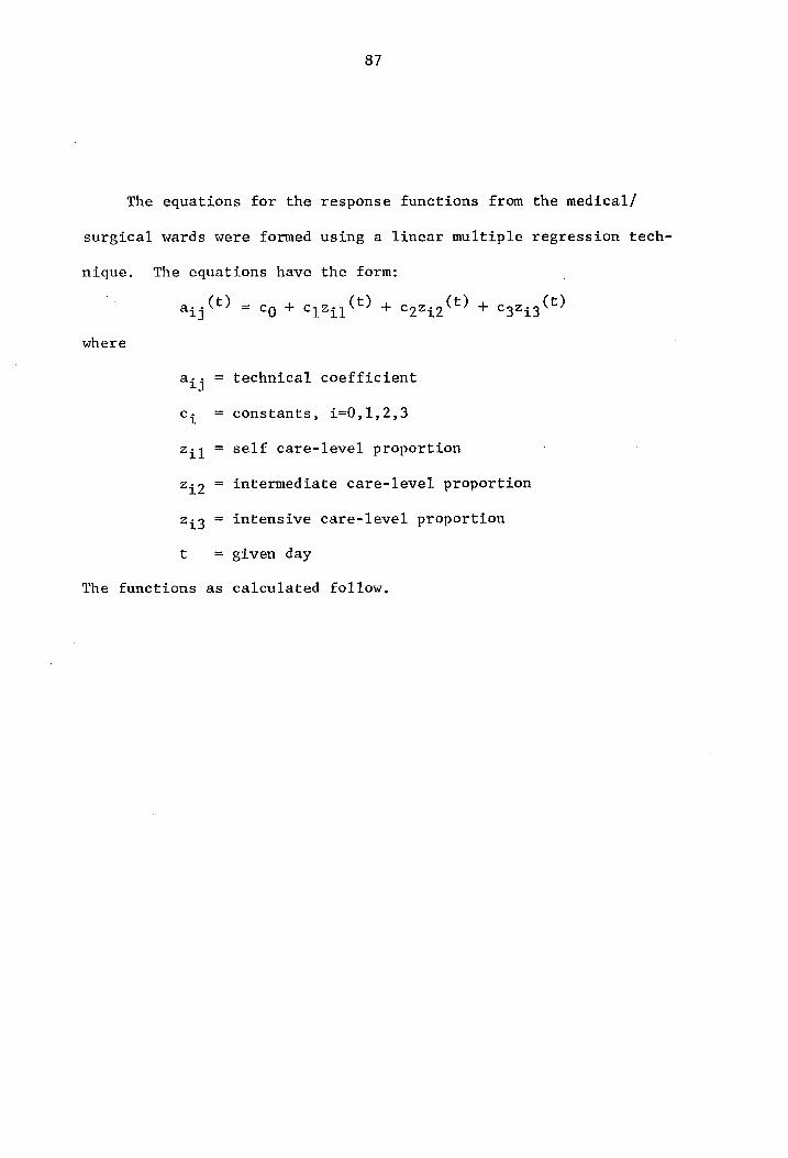
87
The equations for the response functions from the medical/
surgical wards were formed using a linear multiple regression tech-
nique. The equations have the form:
a, 46
where
aiy =
Cc; =
451 =
2452 ~
443 =
t =
The functions as
= eg + ¢42446t) + e249 6F) + cyz546©)
technical coefficient
constants, i=0,1,2,3
self care-level proportion
intermediate care-level proportion
intensive care-level proportion
given day
calculated follow.
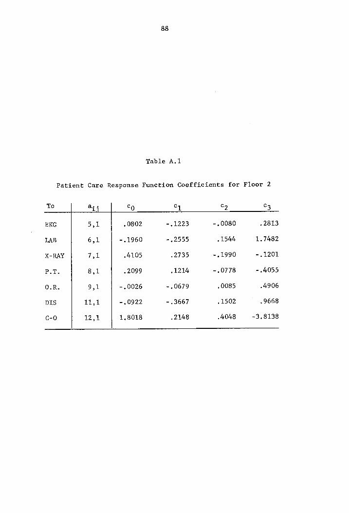
88
Table A.l
Patient Care Response Function Coefficients for Floor 2
To aij Co Cy C5 C4
EKG 5,1 0802 -,1223 - ,0080 2813
LAB 6,1 . 1960 -.2555 ~ 1544 1.7482
X-RAY 7,1 4105 2735 -.1990 -.1201
P.T. 8,1 . 2099 ~1214 -.0778 -.4055
O.R. 9,1 .0026 - .0679 .0085 -4906
DIS 11,1 0922 - .3667 ~1502 9668
C-O 12,1 8018 2148 4048 -3.8138
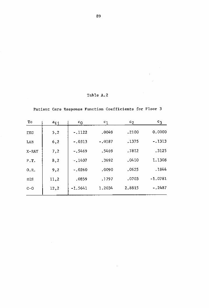
89
Table A.2
Patient Care Response Function Coefficients for Floor 3
To ay; co Cy] c9 C3
EKG 5,2 -.1122 .0049 2100 0.0000
LAB 6,2 -.0313 -.0187 1375 -.1313
X-RAY 7,2 -.5469 5469 7812 «3125
P.T. 8,2 -. 1407 - 3692 0410 1.1308
O.R. 9,2 ~.0260 . 0090 0625 . 1844
DIS 11,2 .0859 .1797 0703 -1.0781
C-0O 12,2 -1.5641 1.2034 2.8815 -.2487
APPENDIX B
Patient Admissions by Care-Level
to Montgomery County Hospital from
November 5 through November 18, 1973
90
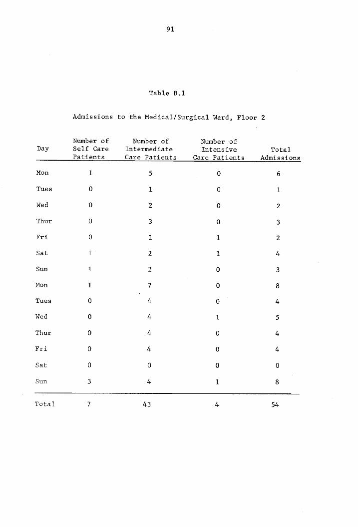
91
Table B.1
Admissions to the Medical/Surgical Ward, Floor 2
Number of Number of Number of Day Self Care Intermediate Intensive Total
Patients Care Patients Care Patients Admissions
Mon 1 5 0 6
Tues 0 1 0 1
Wed 0 2 0 2
Thur 0 3 0 3
Fri 0 1 1 2
Sat 1 2 1 4
Sun 1 2 0 3
Mon 1 7 0 8
Tues 0 4 0 4
Wed 0 4 1 5
Thur 0 4. 0 4
Fri 0 4 0 4
Sat 0 0 0 0
Sun 3 4 1 8
Total 7 43 4 54
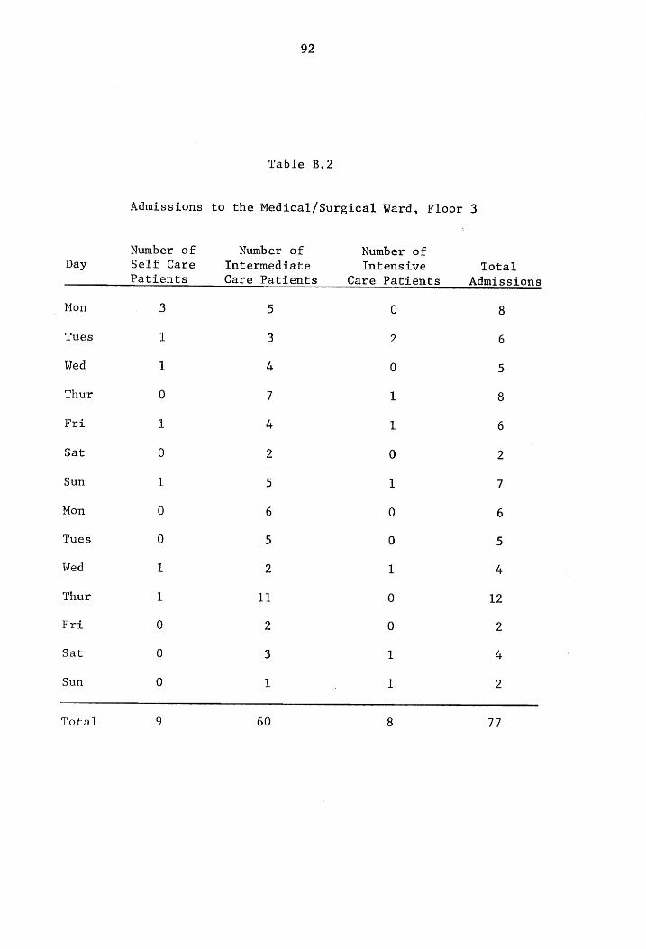
92
Table B.2
Admissions to the Medical/Surgical Ward, Floor 3
Number of Number of Number of Day Self Care Intermediate Intensive Total
Patients Care Patients Care Patients Admissions
_ Mon 3 5 0 8
Tues 1 3 2 6
Wed 1 4 0 5
Thur 0 7 1 8
Fri 1 4 1 6
Sat 0 2 0 2
Sun 1 5 1 7
Mon 0 6 0 6
Tues 0 5 0 5
Wed 1 2 1 4
Thur 1 11 0 12
Fri 0 2 0 2
Sat 0 3 1 4
Sun 0 1 1 2
Total 9 60 8 77
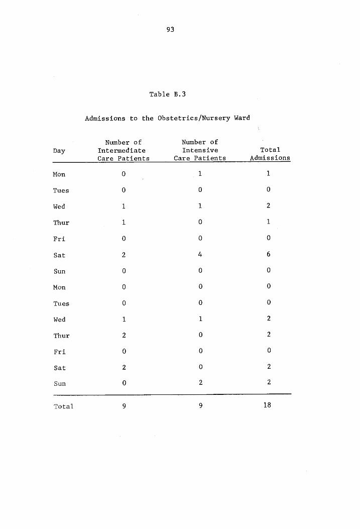
Admissions to the Obstetrics/Nursery Ward
93
Table B.3
Number of Number of Day Intermediate Intensive Total
Care Patients Care Patients Admissions
Mon 0 1 1
Tues 0 0 0
Wed 1 Ll 2
Thur 1 0 1
Fri 0 0 0
Sat 2 4 6
Sun 0 0 0
Mon 0 0 0
Tues 0 0 0
Wed 1 1 2
Thur 2 0 2
Fri 0 0 0
Sat 2 0 2
Sun 0 2 2
Total 9 9 18
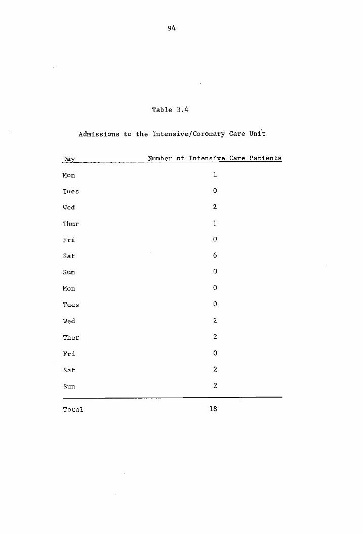
94
Table B.4
Admissions to the Intensive/Coronary Care Unit
Day Number of Intensive Care Patients
Mon 1
Tues 0
Wed 2
Thur 1
Fri 0
Sat 6
Sun 0
Mon 0
Tues 0
Wed 2
Thur 2
Fri 0
Sat 2
Sun 2
Total 18
APPENDIX C
Care-level Proportions, Ward Indices and
Nurse Time Requirements Defined for
November 5 through November 18
95
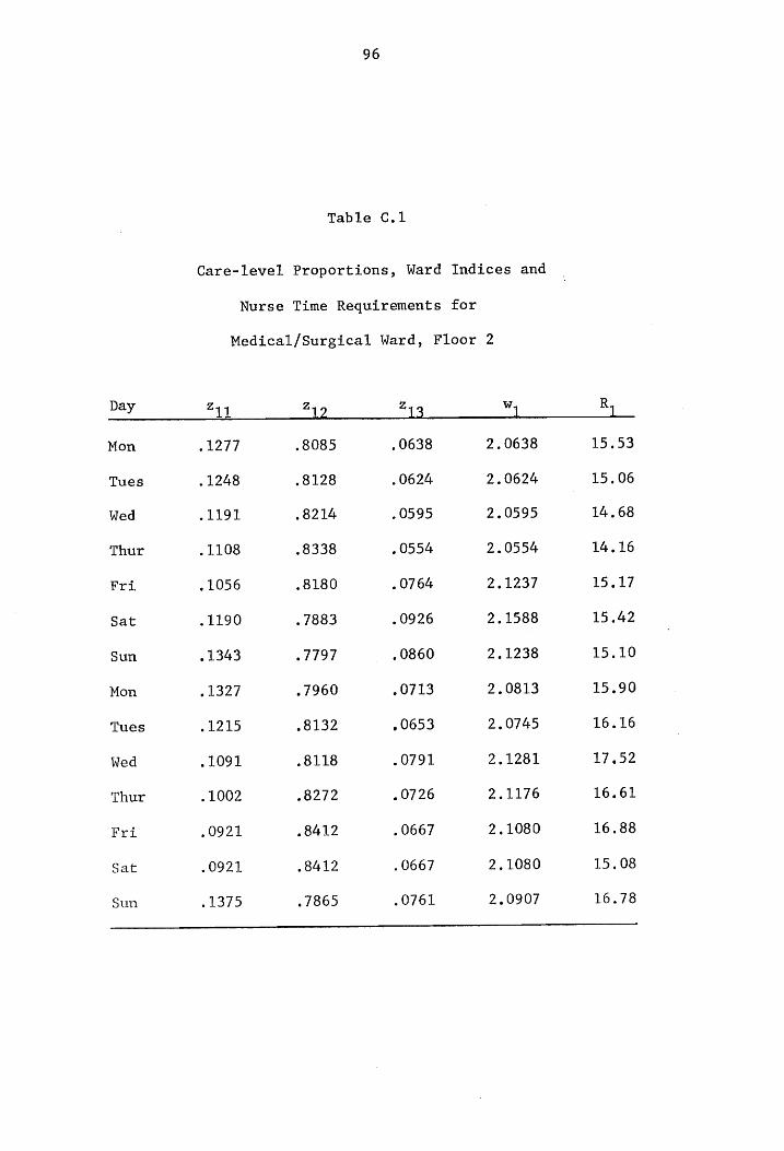
96
Table C.1
Care-level Proportions, Ward Indices and
Nurse Time Requirements for
Medical/Surgical Ward, Floor 2
Day Z44 Za Zaa Wy Ry
Mon 1277 .8085 0638 2.0638 15.53
Tues . 1248 8128 . 0624 2.0624 15.06
Wed L191 8214 -0595 2.0595 14.68
Thur . 1108 8338 .0554 2.0554 14.16
Fri . 1056 .8180 .0764 2.1237 15.17
Sat .1190 . 7883 . 0926 2.1588 15.42
Sun . 1343 7797 _ 0860 2.1238 15.10
Mon . 1327 .7960 0713 2.0813 15.90
Tues ~1215 8132 0653 2.0745 16.16
Wed . 1091 8118 0791 2.1281 17.52
Thur . 1002 8272 0726 2.1176 16.61
Fri 0921 8412 . 0667 2.1080 16.88
Sat 0921 8412 . 0667 2.1080 15.08
Sun . 1375 . 7865 0761 2.0907 16.78
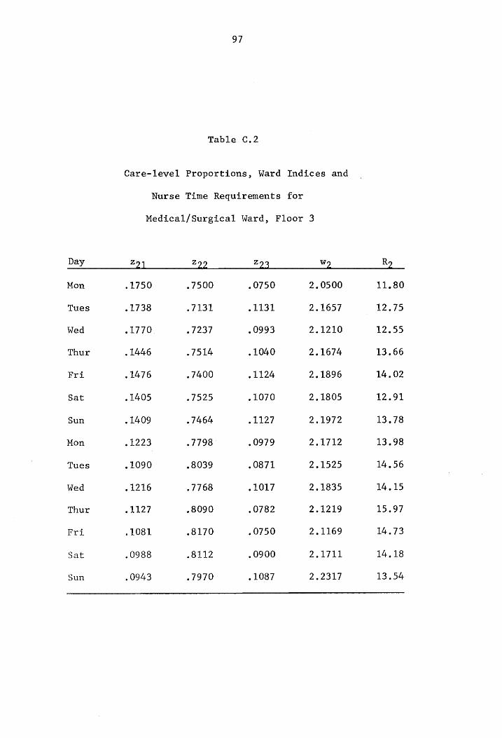
97
Table C.2
Care-level Proportions, Ward Indices and
Nurse Time Requirements for
Medical/Surgical Ward, Floor 3
Day 221 222 223 w2 Ro
Mon .1750 .7500 .0750 2.0500 11.80
Tues .1738 .7131 .1131 2.1657 12.75
Wed .1770 .7237 .0993 2.1210 12.55
Thur 1446 7514 . 1040 2.1674 13.66
Fri 1476 .7400 1124 2.1896 14.02
Sat 1405 7525 . 1070 2.1805 12.91
Sun . 1409 7464 .1127 2.1972 13.78
Mon .1223 .7798 .0979 2.1712 13.98
Tues . 1090 .8039 .0871 2.1525 14.56
Wed .1216 .7768 . 1017 2.1835 14.15
Thur .1127 .8090 . 0782 2.1219 15.97
Fri . 1081 .8170 .0750 2.1169 14.73
Sat .0988 8112 .0900 2.1711 14,18
Sun 0943 .7970 . 1087 2.2317 13.54
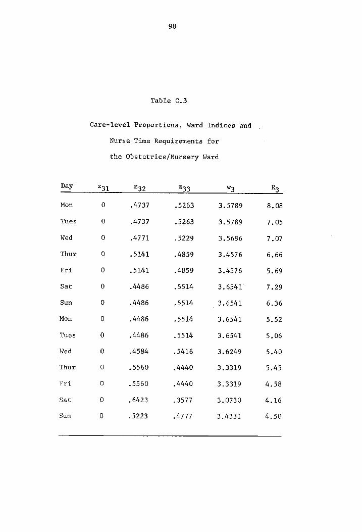
98
Table C.3
Care-level Proportions, Ward Indices and
Nurse Time Requirements for
the Obstetrics/Nursery Ward
Day 231 239 233 w3 R3
Mon 0 4737 5263 3.5789 8.08
Tues 0 4737 5263 3.5789 7.05
Wed 0 4771 5229 3.5686 7.07
Thur 0 5141 4859 3.4576 6.66
Fri 0 5141 4859 3.4576 5.69
Sat 0 4486 5514 3.6541 7.29
Sun 0) -4486 5514 3.6541 6.36
Mon 0 4486 5514 3.6541 5.52
Tues 0 -4486 5514 3.6541 5.06
Wed 0 4584 5416 3.6249 5.40
Thur 0 5560 4440 3.3319 5.45
Fri 0 5560 4440 3.3319 4.58
Sat 0 6423 3577 3.0730 4.16
Sun 0 .5223 4777 3.4331 4,50
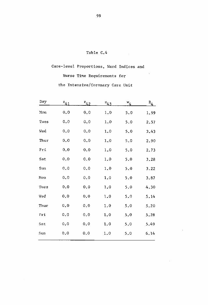
99
Table C.4
Care-level Proportions, Ward Indices and
Nurse Time Requirements for
the Intensive/Coronary Care Unit
bay 241 249 243 wy bs
Mon 0.0 0,0 1.0 5.0 1.99
Tues 0.0 0.0 1.0 5.0 2.57
Wed 0.0 0.0 1.0 5.0 3.43
Thur 0.0 0.0 1.0 5.0 2.90
Fri 0.0 0.0 1.0 5.0 2.73
Sat 0.0 0.0 1.0 5.0 3.28
Sun 0.0 0.0 1.0 5.0 3,22
Mon 0.0 0.0 1.0 5.0 3.87
Tues 0.0 0.0 1.0 5.0 4.30
Wed 0.0 0.0 1.0 5.0 5.14
Thur 0.0 0.0 1,90 5.0 5.20
Fri 0.0 0.0 1.0 5.0 5.28
Sat 0.0 0.0 1.0 5.0 5.49
Sun 0.0 0.0 1.0 5.0 6.14
APPENDIX D
Results of the Kolmogorov - Smirnov Test with
Patient Admissions Data from the
Montgomery County Hospital
100
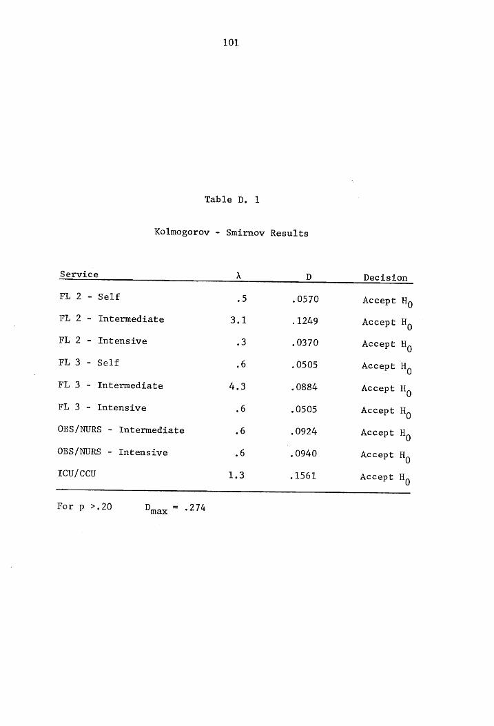
Table D. 1
101
Kolmogorov - Smirnov Results
Service r D Decision
FL 2 - Self 23 .0570 Accept Ho
FL 2 - Intermediate 3.1 . 1249 Accept Hy
FL 2 - Intensive 3 . 0370 Accept Ho
FL 3 - Self .6 0505 Accept Ho
FL 3 - Intermediate 4.3 . 0884 Accept Hy
FL 3 - Intensive 6 ~0505 Accept Ho
OBS/NURS - Intermediate 6 0924 Accept Hy
OBS/NURS - Intensive .6 0940 Accept Hy
Icu/Ccu 1.3 1561 Accept Hy
For p >.20 D = 274 max
APPENDIX E
Computer Program Documentation
102
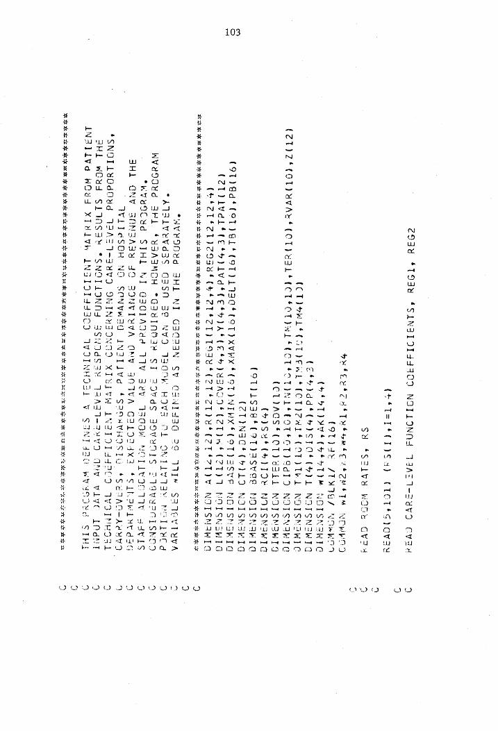
103
cOdd
fTO3u
fSiNSTIIS49093
NOILINAA
TIAZI-24v2
avaHx
(S*T=TS€T)Sa)
(TOT*§s)avay
Su *StiVe
woe
CVi4
DHFEUET
ALT EMEC UEZM ETE
NOW HOD (OT)
FE /THIES
NORE] (ho
oT Ue
(ee eTye
bose dddS(HISTAS
(Hyd
(CT )OwWL
COT IEWLSECTIZHL
SE COT Tea
NOTSNAWIC
NOPSNSWI9
NOTSNaWIC
(ZSTIZECOTIAVALS (CTIEILSCOTEOTI WLS ECTEOTINISCOT&EOT) SGI)
NOISNIWIC
(CLTIAGCSS (OT)
S2Lh
NOISMNSWIG
(HSH
* CH} TDe
NIISNSaWIG
(9T)1S3e*(9TIASYEe
NOISNAKIG
(ZTINSCO* (7)L9
NOISNIRKIG
C9OTIGdS (OTIGLS
(OT) LISOS
COT) XVERX
FEST INIWY
SE (OT SSYE
NGISMSRKIG
CZTIAVALE
CES HIV
AS CESH
IAS CE
SH) ABACIE ZT
Iw EC
2ZT) TD
MOISNSHIG
(ESOT
ECT ICOSeS
(CHEAT EZT
TIF
fC 2T
PZT es
e2T eet)
NOITSNAWIG
BER
RR I
eR
Ae SEK Sk
ee
ie 3
Se oie ak a
aie ie 3
ok a
a aK a ce ake ak ae
ok ake ak akc ak att ac tr ale
ae oie ole
ok ate oh ok ake ote oe oe
BORE ME GA ASR
RC SE ESE OK
Eo
fave oNdd
SHL NI
G3CS3N
SV CSNI1S3G
29 VWIIM
S276 VEMWA
"AISLVeVd3S
G3SA
358 NVI
W30%W
HIVES OL
ONTLVTSY
NOTLwed
W¥¢UOOUd
SHL SYSASMOH
*OGSadTNSIAM ST
FOVdS
F9VUDIS
FIAVYZCISNOD
“Ww¥d9Cdd
STHL
NI G3Q1A0e¢dd
WIV Sey
TWRGOK NOTLYoO WY
s4rls
SHL GNV
SNNSASY
AD JINVIBTA
OMY FAN
TIVA GALD24KR
“SLL Swinrd3ag
wisi WileSOH
NO SONVWAd
INFTIVd
§S29xXWHOSTU
*Sa2AG-ACHYI
| *SNOTLYOdO%d
TAATIA3uvd
ONINYZINAD
XISIVH
INATO144909
WOTMNHDS
FHL WCdd
SLINSSY
“SNOTLONG4S
SSNIdS3Y
TAAST=24
99
ONY VIVO
LAdNT
ANZ1LVa
Wes
XTeLyw
INSIDTSASCI
TOINHDSL
¥ SANT
4BG WedODYd
STH]
WE We
2 Se a
Se ee
Se ke a
ale aie ak ak ke oe oe
os ah ake
ke ok oie de de ake
oe gc ak
ke kk
ok nc ar He
ke ca
oe eax
BK ote ris ake of ote ox ce ok aie
oe of ak ak oe ok
ee ey oc) Ow 0 ss a ta

104
| 1VdS(SOTSS)0V34"
(HETSLEC EATER
SEP ET
VAII(HCT SS)
IVa
tvdO
*SLISIA
ENGLLvdLNS
49 eIeRKAN
SHL
Af VBAET-Jd¥I
AG SNIISSTNOY
SGN 4O
YSEWAN
FHL
MO —{ <f LA) hao
im -“¥ OO
J
Re aR 2
2k 28 Ro
a
2 RC RE aK
eR
Re Rk
SR ARE
OR RE SB
OK A OK
OH
BA FR SK AS at
Me A
A SR BR
eT
3
% t
~
ho o-+4 . ii
bat
ml
ret
ACT Yad
AGNLS
SHL Jo
AVG HOVS
804 NIT
Gy34
329 LSAw
ONTIMO V4
FHL
ke te aie A
te ak ote ate Se kk ob ake ok
a ok kt akc ote ake ak
is ak oe ae ok ok
ake oc oe deo
a ae ok ok
oe
ote oo
a
+ *
PRS OR
2
SE FEO
OR HEI
3h EK
(SST=H=TS CES
TAPS
CFS TPASACI) (POTS
s cyay2y
Cc
STVSABT-3U99
AC SANSTLVd
HSAD-AMNVD
SG daeRwAN
AYVILINI
SHE ava»
(CTSTHPSCOTSTEP
FCP STI Ed SII OSCT SS) CVSH
ddI Df
VV LIGSCH
anil do
SVSYV
SDIAG=ES
Wisa0S
SHL NI
INS Piva
Y AG
A2YUxsNINT
Sisecd GvVsy¥
(2TSTHTSOCTICTEF SOP STV
CECTS SONA
(o8S=T8
CE fG=r Cr Tv
(2cTSSicver
(P4rdy
§XTehvw
LNATDTSS9SG9D
TWOINHODSL
dO ShY¥akh
INVISNOD
OVA
2
(ZJSTHPSESTITTALS
(COP Tae
Oe PP
PT
CORE) TCT
(24 T=P
$6
SGHT Ee (HS
Taye Cy
OP STV
TOSe DIC
TOT*
LA us wt ee
iy bd
cL
OOO 22 OO 42 OOW ¢ WU O moO oO ) 2 i
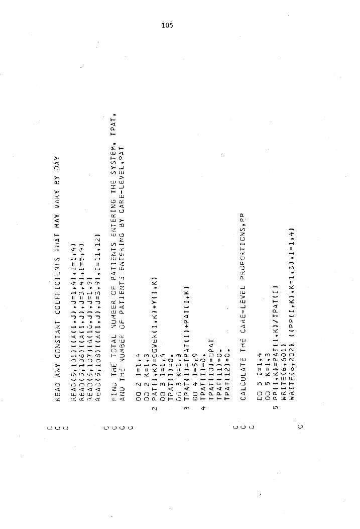
105
fiVdL
(b8T=aT* Cettant
(af rida)
€c0ce*O) ALTUM
(TOS*S)ALITUM
(IT)LVdL/
OFT) LVd= O
S) da
€*Tt=% S
OG e*T=I
¢ 09
dd *SNOULLNGGIUNd
VAAFIA3YVD
SHL FLVIANDIVI
"O=(CTILVdL
"O=(TTIIVdL
IVd5=€CT)LIVdL
(MST Lvdt
CTP LVG
L=CT LVL
(HSE DAFOHSTPHSADDHRCAS
TLV
IVa TBAB
1T-239V9 AG
ONT HSIN
CLNSATLVd
JO
fW3ISAS
FHL ONTYSINS
SINALTLVd
dO eagkAN
*O=(1}AVdlL
6*S=Ii 4%
Oa
EfT=H
€ CO
"O=€T)LVdL
7*T=Il €
€Q
E*T=H% ¢
CO **T=]
¢ Od
42GKNN SHEL
ONY Wwidl
34L NIG
(ZTETT=HTS
(6S ESP SCF STI VI
C8OT SS) CVaY
(6*THP SEP
SOTIVIELCT
IS) QVSe
(59G=TS
(bf E=K
PCF FTV
CICTSE CVI
(OfTHT (VS
Tar SCP
STV
CTOT SS
Ova
AVG AG
AYVA
AWW LVHL
SINSIT3TAS393
LNVISNOD
ANV CVae
LEN
Www C2 Wo)
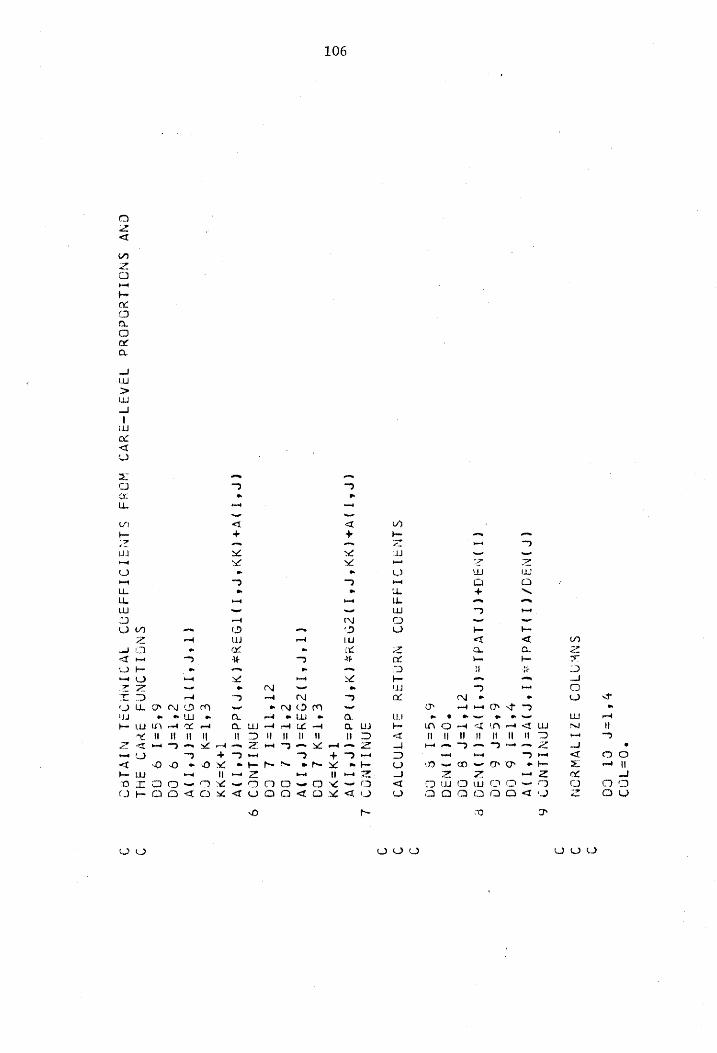
106
°O0=T109 4*T=f
CT Ca
SNKAIOD
S2ZLIVAYON
SANTLNC? (PINFO/CIVLVGLEEL
SP IVECR EDDY 6*T=]
6 Ad
| 6*C=F
6 20
CLYNDOH(P
DLV Ls (PST) v=( T
NA
zt‘t=f ¢
ac "O=(T)N3Q
6*s=1 8
Od
SENSTSTSAS0D
NYNLSY
SLY INOW
SANTINO
(FET IVEC
HHS ET) 7924s
ONS dad
=th fy
T+H=> 9
€*T=x% 2
09 (TAF
FTV COSM=K(K
STD V
e*t=f
2 9G
fTf‘TIT=I lL
CG AANTINCD
CPST IVECHY SPOT
TIS ACEP
dd=(f
STV Te
Heyy
€*t=y
¢ C0
(TEC fT TISUHEL
STV
cf*t=f 9
OQ &*o¢=1
9 00
SNGILINO GS
3Y¥VD SHL
CNV SNOTLYOdOUd
WSAFI-24V9
WOsd
SINSTOTSS399
TWOINKOSL
Niviee
2 OO WOW oO to ©
“T=CF4ST)S
OT €ft
GL O9
— CF
ST)VV-=OFST
DY eT
OL DOF °G3°T)
AI et‘t=f
€T CG
cl*Tt=!i €T
0a
VAAD-ABHVID
YO SsOHVHDSTG
w4AHLIA
OINI
NGTLdvOSaY
dG SATLITIdvsoud
SHEL GNVY
HCLOAS
VY NI
SSwWIkt JO
YAGwAn
Gald3GXA
SSATO
2
*XTeLVW
SJSNOe¢S3e% With
ANIG
(ZTSTHTSOCTS
TRACE EPS TV)
Ce OCfOFSLTUM
woo Ob
107
(STZ*SS)SLIUM
TT (€€02789)3LTUM
ANNTINCS
CIND/EF ST I
VECP EDDY
clft=]
474 GG
ey OL COC*T*
OS" 2109) AI
(F*I)¥42109=c109
cTlf‘t=I €+
O00 "0=2
7199 6*G=f
¢@% Od
SNNTLNCS
TICI/NV
LS (PS PIVACK ST)
7T*G=t
2T 00
OT OL
JOCNVEIS*OS* TWO)
(Pf FV4TIOI=TICO
Z1*c=I
Th CO
TOO-" TENVIS
(fF *T)V4I09=109
%*T=!] IT
7G "O=T
HD
2b nb
€4
TI
108
(ETZ*9V3L1UM CoS
Tar Ces
Tans (er
ypegaoay) (ZOZ4O)
SLIM
(LOZ4O)3LTyM OPV
dde (P1192
OFF) 8SACD
€*T=y¥ LT
OG y'T=f
1T CO
CP YLVdLe
(PS 2TIH=CP
ILD (FILVd
Le (LETT MHIP ISTO
5*T=f OT
OG
YAADD
S$ TIAZINABYVI
AC SHUBAD-AYYVI
GNV 419
SSH3AG-AdYVD
STG
4‘sa9uvHIS
IG JO
YAGWAN
SHL JLvINawWD)
(CTST=TS(CINZ)
(70289) SLIM
(ST2°S) ALINE
(9OcfC)SLTUM
ANNTLINCGS
dwWwiit+(I)Z=(1)7
(PULVdLe (FST) d=dWat
cTl'T=f
ST Ca
“O=(T)2
et*t=iI
St ca
2 *¥OLIS
HOVS
YO4 SONVHSG
SLiv Ino?
CCTSTHTSC2TEITAaP
SOR ST
4D)
(O74 O)SLTUM
(STe*Opalre%
Pr (SO¢*9)3LTu™
CTdGAT fw
* T4C* NFS) ANIW
T1093 POT=I1dAI
CT=N
SANTLNGD
itl
oT
c t. I
Oyu o oa

109
(PFyLvdi* (FILISCL SIA
SANTINO}
Le (FUCSOSLTUM
y*T=f
A
OG
110
(Ff TiWl=aWal
OT*‘t=f
Tes Ca
"“O=(T)USL
ST*T=I
Tos aA
(CTSTHTS (1ST) Gd19)
(2224'S) SLIM
(TZ72*°S)3LIGM
(PE CCSOVSLIUM
COTS THPS(OTSIALS
ORS TWh)
€27278SPSLIUM
(T2éc*9) SLT
U4 IT
(@22*S)31L
TUM (CIGAITSTIGATSIGAE
SV Ti
SUN
SW Sad
I DNL)
GtdKkS
T73
OCT=ZIdAI
COL=LIdATI
COT=IdAI
OT=VN
CT=V1
Ol=VW
(ISP )Y=CP STINE
OT*T=f
O05 OG
CTf£T=I 905
0a
GANTVLS0O
ST ‘Hal
4¥O43SS
HOW3
vOd LNATLVd
YSd CALVYSNIO
SANAAZY
G3L939dK3
WICL
ZHL “ET
wos
ONY LSYTS
CALVINIWI
SI {Wl
§3NNSARBY
G3L99axXS
4D XIULYW
AHL
BUR RICO
ACR SI
OR AE
ICRC ICICI CIC
SO AOR
ESIC GOK
CK CRI
ZO a
aC aC EASA a aa
aa Soc akc ae at Hee
fe ake okese aa
SWISS
KON WYeOO¥d
FHL SO
NGTLISS
Taddw
LSGD
ZHL *NSAIO
R23
3AVH
T20CH
MOIS
LNSTLVdG
TVLIGSOH
JHL WOH4
SLINSAY
SHE INTDG
SIHL
Jv
3M
CE
Se a
sk eo
oe a ok
a oe ke
ae ok ae ake 3
ASK RE S
R
RR RH SRK
rie Oc abe oie ate
Ig a ok ak ok ote ak ae ae ok ak oe ok ahr
ec ok or ok ogc ok ok ake aie ok
ae ok ak ok
ChS
WOUYUOUDOVUOVO YU
111
CT*T=I
€0¢6 a0
ze (14
F)9qII=(1)
ZW
OT‘T=1I
zoSg Ca
(EIGALSECIGAI*I GALS ott yy
fy N*TWHE dai *GadIDIGdahS
ANVD
OT=CIdAI
T=¢1
YUVA
SG2LVINIIWI
ST JANSASY
4D ZINVIYVA
AHL
(CT) YSLIFA3YOL=ASYOL
(O°THTS(L)IDY)
C22749)ZSLIUM
(9eC8
9) AILT UM
(I) TD¢4ASYOL=ARHO]
(T)eSLLte
CT) LIeC 1 Sy=CT) 198
b*T=I
ecs OG
GOTddd
AQNLS
FHL YyOsd
SARYOL
SGSLVIVHNDDV
SI SNNAASY
Tied
JHE “G3L92dX3
SAN3A3Y
WL9L
SHL ONINIVINOD
*19¥
*YOLIAA
MIN VO
ONTWYOd
SQVW
MON 3YV
S31iVe WODN
2HL JONIDNI
JL SLNSRLSAFaY
(|
am Tf t=
mr CTYYSLL)
(2225O)3LT
UM CTET=IS
(I) e3L) (27249)
3LT UM
(T2c*9P3LTUM
(ecc*O)3L
TEs (T)ivolsx(T)H¥Sl=(1)yxats
OT*T=1
SOS G9
T
QaLVINIWI
ST *y¥SLt
GALVYHAN29
JNNSAIY
WLOL
JHL LAdNT
ANSILVd
SHA AD
MSL INIATGIL ING
AG
SANTINGS
dWwI1+(T)¥3L=€1)
21
’ 4 rod
w) aN in
wc OW OM OU O
112
ASxOL
(6¢02*O9)31LTUM
(CTFST=IS(TIAGS) (2225S)
3tT ym
(C27°O)P3L1UM
(CTSTH=IS
CT) UVAY) (22749)
35 TUM
(To?2*9PSLIUM
(72cS9) ALTIUM
CTVLVdLe
(CTD AVAM)LYOS=CT AGS
GWIL=€T)YVAd
(Tl) dVAd-=dwW3k
SCS OL DDECTLOT
EL) UVAY)AI
OTfT=1I 99¢
OG
NIVLSS
ST SANSA3%
T¥L7L
FHL JO
NDILYIARG
GHVINYLS
Cex (T)YSl-CT)eWwl=(
IT) YVAY
CTS1=I
re
Oq (CC IGATSETAGATSIGAT
SOT yw SUNS ow feud ONE GYawS
TI103 (TYCWIi-C
TIN Le ?=( 1
ews
GOOG
ou
113
JANTIINGD
ZOE CTI
LTIOS CIYXVKEXSCIINIANX
SC DISSVES
(TT16*S)ava"
. XW*T=]
70€ GG
GE SN*°XW
(00064S)GYVS3¥
(AQSQNIINT
36 QINOM
37S
d31S
WAWIXYH
ONY WOWINTIW
Vo SWVY9OUd
HIYVSS
NH3LLV¥d
HYBHLQ NI
fT aL
dynes
SVM L130
WVN9DNd
STHL
YO4)
°3S71S d3LS
SHL *479¢
SVEN
ONY "AVSATLIAGSSa
fXVWX
GNV NIWX
“SSTGVIYVA
AHL GCaMOTIY
SSN TVA
WOWIXVW
ONV WOWENIW
SHE GY3u
°aSvEe9 “SINIVHILSNDD
ALTVVNOINI
dO4 ATSISVSS
39 LSNw
SNOTANIWOS
AVILINI
avay
Sd3LiS 3D
YSGWAN
KAWIXVA
SHE GNV
§xXWw “SSTGVIUVA
JO Y2SKWON
BAHL avay
(PSTH=P
SCOTS T=TS (Pry)
) COTZS9) FLIES
(602°9)SLINM
(OTCSOPAILIUM
(OSTHPS
COTE THTS CP STAY)
(COTZ*O} SLT
(602*9)3LTu™M
CEBOC*FFALIUM
ANNTLINES -
"QEOS(FIVZEITOGH(E
SR) dda LETH (ZL) dde E
ST Pi ddti2ya(P ll yyy
(ESP) dd
SHI ZSP
dda’ ZtOT
RP) dd=treLiye b't=f
T og
MV SSALYWILS3
SINSRAUINASM FHL
GNY 44
*S3DTGNI Guys
3HL aivInoaqy)
We ORE
RE a
AR Re
a a aC
ai ae
ote ee
te ee
ke ode aie aN ak ke ake
ea
sc ak
ok ake
ec ak oe ote ok akc
ne a
ak abt ok oe le ae oe ak al okt ok
ate ot ok
“T30G0W
NOTIVOOTVIW
4dVLS
SHEL HLIM
GANS39ND9
ST WYMO0ud
SHI 49
YSONTIVWAY
FHL SSELINS3e
WdQW
1599
YO4 NGIL93S
3HL SIGNIINDI
STH
RR Ze
Re IE
SC
5K Se ak ae
RC A Ke
ak oe
aka a
aR oie
Xe ak os
a a
a a
ok ake eo
ake oke ae ake
ae
ae ae ake a
ake
OOOO VUOUOO oO WOVUVD OO WOU
114
9S .
T=rr SS
O2ex °OT-=XVRA
9S |
T=3I
(Il}4u=¢1)Gd
(T)4y=CT)
GL (IJ4¥=C1)3SV4
XW'T=I
SEE CA
CTe€e OL.09
*T=May
| IT
Si whoa
13S ST
*M3u *
NOTLNTOS LwNS
3HL YCO4S
LNVLSNOD SLNIVYISNOD
sHL
T=3S1 IANIANOD
6% (IL)
3SVA=(1)84
87 (Ty3SVG=(1)4y
LY (IL)SSVG=CI)VEL
(1)aSvag=(1)asvea
XW éT=1I
90€ 5a
BE C=H3LIN
"ocT=a@e Te
T=ONI (>*NnT)M=OM
(oc SNwWT)M=EM
(2°NwT)Mseé
CT SNA
T)M=TM
(7 SNA
T)VEbu
(E Ne
T) VEER
(2°NEV) WV=ECu
(TSNWT)V=TX
FITfST=Nw 1
206 CG
WOO vd
115
cot cOT
COT 66 85 96 €6 26 16
06 98
98 €8 c8 BL
GL SL VL
el cl TL OL 69 S9 19
6S 8S LS
Xw*T=I
OTT Oa
c=FP
TI‘ (ocotfoet)
O11 69
SANTINO
c=II
C=YISLIN
fl)su=(1)1Ss9
AAK=XVWA
C6 G1
Q9 (TIGL=(I
psu O08
OL Of
(XVWATLOSAADSI
AAm=KA
(MASSAASONTISASENS
VIV9
CTONTWX=CT)
Gea CODINTWX*
17° C1) 4¥)4I
(T)LIZG-(T)GL=¢(T)Se
98 OL
99D tXVWATLOSAADSI
AA~=KA
(MAXSAASGNTISASENS
WWI
(TUXVWX=( TIS
COCDIXVAXT
LOOPED AN) AT
(T)f7430+(T)d1=(1)44
XWST=1
06 Od
C=TT
(TPANS
FF) AA=XVWA
(T)ae=(P)1S3¢
XW‘T=I
OR2 09
C=qdalINn OL
OL OCD
CXYWATATPAADAI
AA-=AKXK (MAX fAASONTIISASENS
1149
(T)8i=(1)
44
XW*‘T=1I €9
Ga T=I1
CCT
Ob " 2 Oy
ev"
wy
116
set
OTT cll
69T eoT LOT 990T
SOT vOT
CCCOT) SXF
EOP AUF
(ZAI
-CUuISEV/( (COT) 38409)
S84 02)
44 )-2e) -€67T)
SESH
TO€ OL AS(GED**
LO HH) Ay
(C6 )SU4(GISNFT)SHI-TY)SEV/
(0 ( (6) 444 (6)
dee CTY) -Te)
ET) aed
TO? OL
OD(SCO*PLO*
CH) AT
“em CCTIAN+ETT
See OT) su4(6) 4H=8H
TO? OL
DO(SCO**19"
ZH) AI
"T2-(S)4adt(L)444+(9)
44405 )44=7H
TO?
OL INCSOC**LO*
TH) AT
“PT—(Y)
dee (Ed
SNF (7)
4u4(T)
44 =
TH
NOTLINIGS
HDUVAS
VYSLLVd
SHL 49
ALINIGISV34
WO3HD
T=ONN (CT)
LS3@=¢1)4¥ Xw*T=I
€€€ OG
XVWA=E 902
OL O9(TOOCOTO**
AT 4raG)AI
(GE-XUWA)SEV=4IC
O02 OL
COCAE OAK YWA)AT
NOTYSLTIYD
ONT ddSiS
¥O3HD
SANTINO
cs OL
29 T+3T=3]
C@T Cl
GSCSN*S3*°OLD)ATI
JANILNED
CTUXVWX=C(T)GL
(C1) XveYe
LOT (ISL
SI CTONIWX=(€TIGL COLINTWX*T
LIS CIAL
AI (LiSd-(CT)2SVAx
CHC T)EL
(P)Av=C1)2SVE
(L)3SVG=(1)Ee
re my
my
COT
Qo) Oo Qo
117
(HS T=TSCT)LS3E)
(O€08
49) 21TUM
(6C96*S)3LIUM
XVWASNWT
(O890649O)31IHY
9E1 JANTINGS
Cty OL
09 T+3S1=251
"oH /MAUEMO8
LNVISNOD
SLNIVALSNGD
43N
Waod
STAISVGHNI
SI NOITINIDS
41
co@ O1
09 TO2
CL DECTOTLASBO)ST
(2T)3eeOS*-(
(8) ANF (H) Su) KOT*=89 TOZ
OL FOC
OTLINL9) SI
CTT) dtxSS°-((L)Se4F
(EC) 4d eSH
HLS TOZ
OL O9C°OTLTS9N)
ST COT) AGROI=-C09
ALF OZ) SY) x04 09
TOZ CL
B9CTC*LIGOD SI
(6) AYKOIT—C
UG) ASH
CT) de)
Koes =69
TOZ OL
Q9C°C LITHO)
ST COZTIAL+(BVAII
OS *=0 4) due tGt=49 TOZ
OL TOETCTIIS
ENT
C(TT)SU4 (2)
48) 80E*-(8
Jays OL =e9
TO? OL
2OE O8ETZ9)41
COST) ALF
(DSH) ASE
9- (2 aye
G15 =279
TO? OL
D9e°O"LV°T9)41 C(S5)S4
(SV 4B)
eGZ-CT See
GL =T9
TOZ OL
D9(GCOP*LOT
LH) I
CCCCT)4d4 (8
bat (4)
aa d—ba)SOV/(CCZT
444 (8)
do)
de) be)
691) ayer H
To? O1 T9CGCOS*
LOT SH) ST COCTT)4N4
CL) sU+
(CE ae) -EMISSV/
CC CTT)
4u4 (2)
ue (O)
43) 82)
06 T)
ay eoy TOZ
Di DOIGCO**
LO SH) SI
WOW
118
(VISAVG
NO XIMLVW
SNNFASY GALDTdXAHPE
*XZ 4 TA LVRUOS
(QDHZ 4X8
*STOHE*
XZ‘ H3SH2
fXe FHOHZ Ke
SE dHZ
SY KXE SAVY XHS XG Sav
THES
KL FONT
JHE*XLINII/NITIHL* XE*SUNN/S E9HE
* KZ
FE YODWMHL XESS HODIFHL§
XE) LVWHCS
(C°CTSAEV LVR YG
(OSUaINGH2 * XZFYe3AQ
GALYavIHCT
SX? *GA9DNVHISTOHOTPKX2//
) LAOS
(SYOLIVA
ONTLHOISM
SHLHTZ8XZ2//) 1VRNC4
(Z°OTS+T)LVwuogd (2
NOSHE 4£XGSiVSHE é
XG
# TYdHe *XG SNHLHE 4xG*aaMHe
tygsé IN LHE
XC fNOWHE
SX S4NAST
HE *XC SLVSHE
SxG *TYsHE $
ye *Mujue eves JAMHE 4XS fANLHE Sx
NIWHE ©¥5) Lynn
(Q4A0GA3aN SAVG
ASYNANHLTSXZ//) LVWUCS
(SATS2
NS INTH6*S
X? SSL VIGIWYALNIHZT
6X4
Sa TaS He
XLT SSHSADAMNYIHOTSXZ//
FE LVWMOS
(YOLIAA
ALTAITLIV
WLOLHTZ§xXZs/) vend
(C1SAVOQ
NO XTSLYW
JSNOGS3Y
AVLOLHOZ*X2//) LYRYOG
(F°OTACTILVWHOS
(f1SAVCQ
NC SINSIDI44909
WWOIINHISL
49 XTYLVHYHSES XZ//)
LV RUC
(7° 7TSe*xee2) Lvyyagd
(SAISNAINTHB
SX? ST
ALVIGSWYSALINIHZT
SX STESHe
XL SSNOTLAIDGV%G
ZYVO FHLHOZ*
XZ 4 ale PLYWHO (o°OTSL)
Lvwycs (>°
246) 1¥WUOS
(>°CT39) LVWUOS
(4° OTA) LVWUCS
(S° OTIS
VL VWHCS (>*CTS9)
Lywuod (7°S3S)
LVWUoS th
OTIF) LVWYCS
Let LIX]
WIV) SNNTENSD
(ZLSS=1*
(1) 1538) (ZE064S)ALTEM
(24C=1*(1)1S93) €1E0564O)3LT
UM
uce
a
412
ET? ET? CTt2
602
Re?
L0¢ 9t¢
SO¢ 90?
EC? eC?
TC9 OT
LOY QOT SOT 7OT CCT oot TCT
o ?
cnt
119
671
BET
ON3 dQOLts
(S°OTS>) LVwWHOd
TITS (T
V*CTSS=ALIVNGd
HLIM HOTSET®
AVG NO
NOITLYICTIV
JS4viLSHeZ*°xX2//) ivwungd
Cars (6Z0649)SLITUM
(NDISNOTHLS
X27 FSENN/S ADH
ff Xb SC
TSHE SKE
© ZTAHE SXETILYWNOA
6205 (Z°OTS4* SAVNHG
XZ) LYWHNOH
7EC5 (2°OTA¥*
SaNd THs
*xZ) iVWwerg
TEe05 C*OTSAY®
SiNUHG*
XZ) LVHUOA
OFO6 (STS
*XT)LVWYOS
Cres (C°OTH*ST
WLIdSOH
SHL DL
3AWCONT IWIOLHTE*XZ7//) LVRHOS
£72 —
(SHDYVHD SDIAYMSSHSTSXZ//) LVWUCA
622 (S39eWHD
WOOd ONTANTINI
FNNSATYROESXZ//) LYKYOS
922 (SNNZSARY
W1ICL
SO NOLLIVIAIM GYVGNYLSHSE*
X77) VWUdsa:
272 (SNNGASY
JQ JONVIMVAHGTSXZ//)
LvKWYnS 622
(S3NNAASY D3199dX3
WIGLHZ2*xXZ//)ivWwycs
€22 .
(2°CTS°¢
UD ivwyuas
222 (SSH
XefHOHT
SX Lad?
PKR SAV
YR-KHG ENS
HAV IHE
OKs FONT
FHE* XL ANID/NITHL
XE SSUNN/SADHES XZ4E
HOCTAHE SxE*?
YOGIZHE*
XE) LYWurd
122
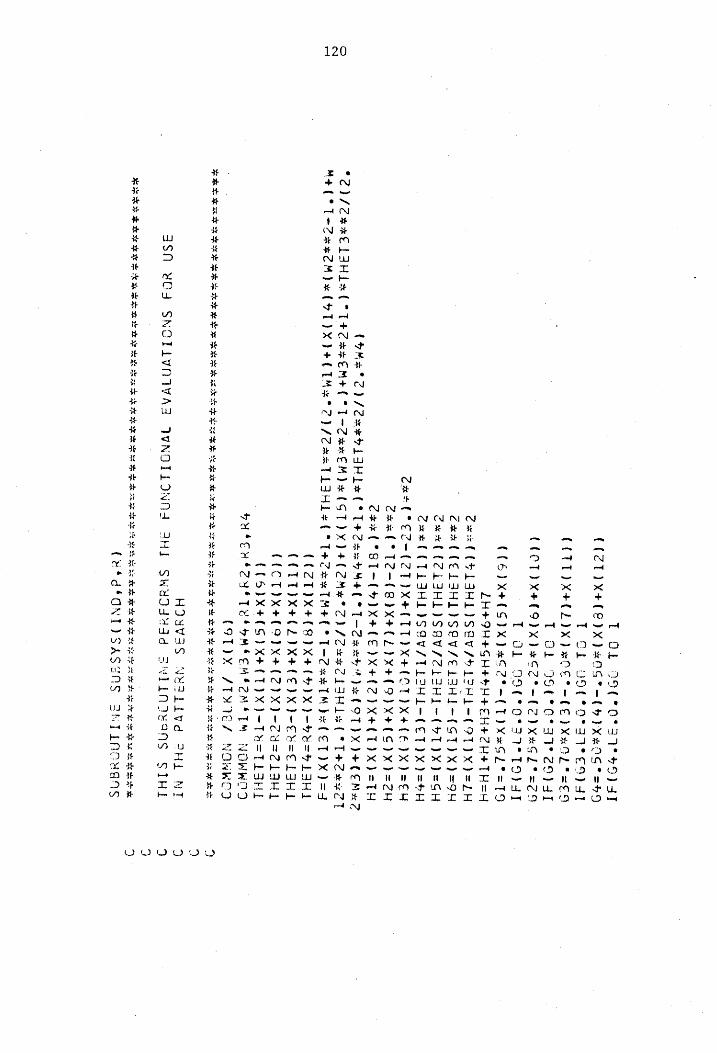
120
T OL
29¢€°O°397"°49)
47
(CT
IX4+(E
XK) RNG
TAH bX KNG THK
T OL
99(°9°37°€9)4T
COTT)X#OCL
YX) OES HCE PKR
THEN
T OL
996€°0°37°
29) 41
(COTIX409)K)*E2°-€
2) KXeGL1°=79
T ol O9¢°
0° 37° TO)GI
(CEVX4#05
3K xO 2°-(T)XeGL °=T9
LH+9H4tGH+4H4+
Ht ZH4+
THEY
Cxx(
(GV LIHLISEV/HLIHL-(9T)X)=2H
Cxx ((CLIHLISEV/ELIHI-(ST)X)
=94
exx((CLFIHLISSV/ZLAHI-(
oT) X) =
GH
Cae
CC TLFIHLISAV/TLEHI-(ET)X)
S6H
CHEE TECH (CT
XFIT
EP X400T X46
7X) HEH
CeXE T2-(BYXFCLIX4°9) X406)X)=2H
Cex (*ST-(H)X4(E)X+(Z2)X4
(TX) =TH
(Mx ZV/Zxev
LIM Le (8 T+ Zee
he (* TZKae
te COT)
XE CEM KZ "CVS CHRELIHL
(CO THCRKEME(
ST -ZaR EM)
IGT)
YX) 4(2MK
OZ) Sex *CLSH Ls
( *T42uxZ
M4 (°T-ZexZM
x (OT)
Xd4C TMK
2) /SZRRTLIHLE
(TT 42%
TMH €
§ 1-2 XIM)x(ET)X)=4
(CCTIX4+°8)X4
09)
X }-bY=HLSHE
CCT TIX4+(2)X4+00)X }-ON=EL5HL
COC TIX4°90X4(2) X%)-Cu=Z19H1
(COVX4(°G)X4
(TIX) -TH=TLIHI
DHS Cus
eye Te
bMS
eM Eom
$s Tm NOWWOD
(9T)X
/THVE/S
NOWKCD
si ok ok
ak ae ak
ok ak aeok
ek
x RRC Re
A TNE OK Be
ak ik
2K ok
ie oe a ak
ig ak ak ode aie ok ate ak
nc ok kc
ck oe oie of
ote ok ak ok oe ote
sit te tk ofc ox Beaks
tok ok ax
stk
HISVSS
NYILivd
AHL NI
JSN YOS
SNOTLYNIVARS
IWNOTLONAS
AHI SWHOS¥Sd
ANILNINANS
STHL
SAS
i ROK
ok a ak ae aie ake ok fe ac ake ot ok a ak
a ote PEPE SE
RRR
SE RR
aR HEE
ee
34 " v)
pm
id a %
lid :
5
sk ak x ‘GAS
AG
* é
«we
OE TEE oe oe
NTLACY
iS Ny
) sf
coe ok oe ok ak
d°QNI
a
x
OOOO OM

121
ONS Naniag
DeUE(M)LUBS /H+4=d
bxxOT=9
¢ GL
29 ROS
PTHELOS ET
ADIOS EO T
4S9
SO THe
OS STH
ES / OTH
Z9/ * TFT
OS 9 TH9
T OL
29OE*O"IRI1T O9)AI
CCT)X*9G6°-
CFP) X4F09)X)*9TPH89
T Gf
COC*OC*AWLO)}AYT
€TTIX#SSG°-(€L)XK4+05X)
kGb
8 HL9
T OL
[90°C 837°99)4T
(CTIX*N9"°-( (9}X407)X ne
=99
T OL
O90°O°37°S9)4]
(E)X*O09°-((G)X4(T)X)
aoe r=¢9

VITA
Richard R. St. Jean was born December 1, 1949 in Leominster,
Massachusetts. He graduated from Notre Dame High School, Fitchburg,
Massachusetts in 1968,
In September of 1968 he entered Lowell Technological Institute,
Lowell, Massachusetts where his B. S. degree in Mathematics was con-
ferred with honors in June of 1972. He entered graduate school at
Virginia Polytechnic Institute and State University in September 1972.
He has been honored by election to membership in Tau Epsilon Sigma and
Alpha Pi Mu. At the present time he is a research analyst with the
Mitre Corporation at their Bedford, Massachusetts operations.
Richard is married to the former Joanne Bilotta of Leominster,
Bellacd ® San
Massachusetts.
STAFF ALLOCATION AND COST ANALYSIS:
APPLICATION OF A HOSPITAL PATIENT FLOW MODEL
by
Richard R. St. Jean
(ABSTRACT)
In this thesis the applicability of a hospital patient flow model
is used in addressing hospital resource allocation problems. Three
separate but interrelated models are presented. First, the hospital
patient flow model is discussed. The main feature of the hospital
patient flow model is the matrix of technical coefficients, which
gives the probability of patient transfers throughout the hospital.
Given the hospital system's daily patient input, the model provides
the patient demands upon the different hospital services.
Results from the patient flow model are used in the development
of a staff allocation model. The staffing model involves the mini-
mization of a weighted quadratic penalty function. The weighting
factors are based on the proportion of patients in each of three care-
levels in the wards. The weights are also dependent upon whether
overstaffing or understaffing is the situation. Constraints to the
model include a desirable mix and number of the available nursing
‘staff. Solution of the allocation model is obtained by using SUMT
with a pattern search.
A third model concerned with predicting hospital revenues is
presented. Again, results from the hospital patient flow model
are used to present estimates of the expected values and variance of
a hospital's revenue.
To illustrate the use of the models, results from a two-week
study period of the Montgomery County Hospital are presented and
discussed,


![Cost allocation joint cost [compatibility mode]](https://img.pdfslide.net/doc/110x75/54448861b1af9f740a8b49b9/cost-allocation-joint-cost-compatibility-mode.jpg)