Embed Size (px)
Citation preview
INSTITUTE OF TRANSPORTATION - TECHNISCHE UNIVERSITÄT MÜNCHEN
MASTER’S THESIS
Stated preference survey design and pre-test for valuing influencing factors for bicycle use
Author:
Heather A. Twaddle
Supervisor:
Prof. Dr. Regine Gerike (mobil.TUM)
München, November, 2011
M.Sc. in Transportation Systems
INSTITUTE OF TRANSPORTATION - TECHNISCHE UNIVERSITÄT MÜNCHEN
November 11, 2011
MASTER's THESIS
for M.Sc. candidate Heather A. Twaddle
Date of release: July 11, 2011
Date of submission: November 4, 2011
Topic: Stated preference survey design and pre-test for valuing
influencing factors for bicycle use
The master thesis is supervised at the Chair of Traffic Engineering and Control. The
student has the responsibility for his or her work. The Chair of Traffic Engineering
and Control declines any responsibility of the research and findings of the master
thesis.
Date: Signature of Supervisor of TUM:
UNIVERSITÄTSPROFESSOR DR.-ING. FRITZ BUSCH
Arcisstraße 21, 80333 München, Tel. (089) 289 – 22438

ACKNOWLEDGEMENTS
I would like to thank Prof. Regine Gerike for giving me the opportunity to work on
such an interesting and challenging project. Her extensive knowledge of survey
design and bicycle transportation as well as her support throughout the last four
months contributed enormously to the success of this thesis.
Thank you to Thomas Wagner for his work in organizing the survey and for his
stupendous translating skills.
I am very grateful to Daniel Markus and Raffaela Riemann for the time they took out
of their busy lives to help me edit and improve this thesis.
Thank you to all my family and friends in Munich and Calgary for everything you
always do for me.
Many thanks go out to the 48 people who took the time to fill out the time-use-travel
diary and extra special thanks to the 44 who then completed the online survey. I
couldn‟t have done anything without your help.
Last, but surely not least, I am indebted to Jakob Huber for his tireless work folding
letters and stuffing envelopes and for his endless support and encouragement of my
work.
Heather Twaddle
Table of Contents Abstract ...................................................................................................................... I
1. Introduction ........................................................................................................ 1
2. Literature Review ............................................................................................... 5
2.1. Bicycle Transportation Research Review ...................................................... 5
2.1.1. Built Environment ................................................................................... 6
2.1.2. Natural Environment ............................................................................... 7
2.1.3. Socio-Economic Variables ...................................................................... 7
2.1.4. Psychological Factors ............................................................................. 8
2.1.5. Transportation Related Factors .............................................................. 9
2.1.6. Destination Facilities ............................................................................. 10
2.1.7. Remarks ............................................................................................... 10
2.2. Review of Choice Modelling ........................................................................ 11
2.2.1. Overview of Choice Modelling .............................................................. 11
2.2.2. Remarks ............................................................................................... 14
2.3. Review of Stated Choice Methods .............................................................. 15
2.3.1. Selection of the Alternatives, Attributes and Attribute Levels ................ 15
2.3.2. Experimental Design ............................................................................ 17
2.3.3. Full Factorial Design ............................................................................. 18
2.3.4. Fractional Factorial / Orthogonal Design .............................................. 19
2.3.5. Efficient Design ..................................................................................... 20
2.3.6. Building SP Experiments from RP Data................................................ 24
2.3.7. Remarks .............................................................................................. 26
3. Research Methodology ................................................................................... 27
3.1. Sample Recruitment .................................................................................... 27
3.2. Time-Use-Travel Diary Design .................................................................... 29
3.3. Time-Use-Travel Diary Distribution and Collection ...................................... 31
3.4. Coding the Time-Use-Travel Diaries and Estimation of Non-Selected
Alternatives ........................................................................................................... 32
3.5. Stated Choice Survey Design ..................................................................... 36
3.5.1. Relevant Alternatives, Attributes and Attribute Levels .......................... 36
3.5.2. Model Specification .............................................................................. 45
3.5.1. Using Revealed Data to Create the Stated Choice Experiment ............ 47
3.5.1. Segmentation of Respondents ............................................................. 47
3.5.2. Experimental Design ............................................................................ 50
3.6. Personal Survey .......................................................................................... 60
3.7. Stated Choice and Personal Questionnaire Distribution ............................. 61
4. Results .............................................................................................................. 62
4.1. Response to the Survey .............................................................................. 62
4.2. Time-Use-Travel Diary Results ................................................................... 63
4.3. Stated Choice Experiment Results .............................................................. 66
5. Discussion ....................................................................................................... 70
5.1. Sample Recruitment .................................................................................... 70
5.2. Time-Use-Travel Diary ................................................................................ 72
5.3. Stated Choice Experiment .......................................................................... 73
6. Conclusions ..................................................................................................... 76
List of Acronyms .................................................................................................... 78
Source of Reference .............................................................................................. 79
List of Figures ........................................................................................................ 85
List of Tables .......................................................................................................... 86
Appendix A – Bicycle Literature Review Tables
Appendix B – Invitation Letters
Appendix C – Time-Use-Travel Diary Survey - German
Appendix D – Online Personal Survey and Stated Choice Experiment
Appendix E – Personal Questionnaire - English
Appendix F – Stated Choice Experiment – English
Appendix G – Stated Choice Experiment - Additional Information - German
Appendix H – Stated Choice Experiment - Additional Information - English
Appendix I – Experimental Design
Appendix J – Ngene Code Used to Produce Experimental Design
Abstract I
Institute of Transportation, TU München Heather A. Twaddle, November, 2011
Abstract
The personal and societal benefits of bicycle mobility are numerous and well known.
Quantitative estimates of the influence of bicycle trip characteristics and the features
of other modes of transportation on the choice to travel by bicycle are imperative in
predicting the outcome of bicycle transportation policies and measures. However,
little quantitative research has been carried out to investigate these factors. In a step
towards providing these quantitative estimates, a methodology for a two-phase
stated choice experiment investigating mode choice behaviour based on reference
scenarios is presented.
Revealed choice data is collected in a first phase using a newly developed time-use-
travel diary, in which respondents note their activities and trips from one day. The trip
information collected in the time-use-travel diaries is used to create individualized
reference scenarios. Three alternatives, the car, a generalized public transportation
alternative including the bus, tram, U-Bahn and S-Bahn, and the bicycle are
investigated. The attributes included in the stated choice experiment are the travel
time, parking fee and an all-inclusive driving cost for the car alternative, the access
time, ride time and fare for the public transportation option, and the travel time,
percentage of travel time on dedicated bicycle infrastructure and the availability of
secure parking at the destination for the bicycle option. Pivoted attribute levels are
selected based on the findings of previous research and a
heterogeneous/homogeneous efficient experimental design is constructed. The
sample is segmented based on the mode of transportation reported in the time-use-
travel diary.
The methodology used proves to be useful and statistically relevant. However, the
two-phase survey instrument is found to be cumbersome and work intensive.
Recommendations for improvement include the development of an online version of
the paper and pencil time-use-travel diary as well as automating the coding and the
estimation of the attributes of non-selected alternatives. The attributes and attribute
levels included in the experimental design appear to reflect the choice behaviour of
the car and public transportation users but not bicyclists.
Scope:
The scope of this thesis includes:
a thorough review of previous research concerning bicycle transportation and
mode choice;
an in-depth review of discrete choice analysis and the current stated choice
experimental methods;

Abstract II
Institute of Transportation, TU München Heather A. Twaddle, November, 2011
the recruitment of a pre-test sample of respondents;
the design of a time-use-travel diary and the adaptation of the instruction
documents for the diary;
the distribution and collection of the paper and pencil time-use-travel diaries;
the coding of trip information collected in the time-use-travel diaries;
the estimation of the attributes of non-selected modes of transportation using
online trip planning tools for all the trips recorded in the diaries;
the identification of relevant attributes used to describe the selected modes of
transportation and the selection of appropriate attribute levels for the choice
experiment;
the development of an individualized stated choice experiment using the
reference scenarios defined for each of the respondents;
the creation of a personal questionnaire adapted from personal and
household questionnaires distributed by the Mobilität in Deutschland for
various research projects (Mobilität in Deutschland 2011);
the creation and distribution of an online survey containing the personal
questionnaire and the stated choice experiment;
a qualitative evaluation of the overall effectiveness of the survey instruments,
the distribution and collection processes, the method of coding the trip data
and estimating the attributes of the alternatives and the stated choice
experimental design;
and suggestions for future improvements.
Objective:
The overarching goal of this thesis is to provide a methodology for collecting mode
choice data for situations where the bicycle is included as an individual mode. The
collection of such data would make it possible to understand the influence of bicycle
trip attributes and the attributes of other modes of transportation on the choice to
travel by bicycle. The impact of policy measures and infrastructure design on bicycle
use could then be quantitatively predicted using modelling software. The costs and
benefits of bicycle promotion plans, infrastructure revisions and other transportation
projects could then be more accurately assessed. In working toward this goal, the
objective of this thesis is to design and pre-test a methodology for a two-phase
stated choice experiment using reference alternatives. The entire survey process is
formulated and then assessed beginning with the recruitment of a pre-test sample
and concluding with the data collection from the online stated choice experiment.
The objective is to deliver a qualitative analysis of the effectiveness of the time-use-
Abstract III
Institute of Transportation, TU München Heather A. Twaddle, November, 2011
travel diary, the coding process used to generate the reference scenarios and the
stated choice experimental design, as well as offer suggestions for improvement.
Approach:
The choice experiment is constructed based on the most current methods of stated
choice experimental design, which include the use of reference scenarios to increase
the realism and familiarity of the choice situations. This method has been found to
increase the validity of the choice data and improve the robustness of the resulting
mode choice model. Because trip information from the respondents is required to
create the individualized reference scenarios, the survey is carried out in two
phases. This method has been found to produce excellent statistical results, but
often at the expense of a cumbersome distribution and coding process.
Nevertheless, an attempt is made to reap the statistical advantages of implementing
such a method while minimizing the logistical difficulties. The experimental design of
the stated choice experiment is constructed using a homogeneous/heterogeneous
efficient design. Revealed preference data is collected from the sample using a time-
use-travel diary, which is a combination of the conventional time-use and travel
diaries. The time-use-travel diary is designed to capitalize on the strengths of both
types of diaries while avoiding the pitfalls associated with each.
Introduction 1
Institute of Transportation, TU München Heather A. Twaddle, November, 2011
1. INTRODUCTION
The advantages of bicycling for transportation on both the personal and societal level
are numerous and well known. On a personal level, the bicycle offers a fast,
inexpensive and convenient alternative for short to medium length trips. On a
societal level, problems stemming from excessive automobile mobility, including
congestion, air pollution, urban sprawl, noise pollution and climate change, can be
counteracted by shifting car trips to the bicycle. Furthermore, the health benefits
reaped by bicyclists through physical activity as well as by society as a whole
through air quality improvements provide additional motivation for the promotion and
support of bicycle use. Although the benefits of bicycle mobility are well known, little
quantitative research has been carried out to investigate the effects of bicycle trip
characteristics and the features of other modes of transportation on the choice to
bicycle. This knowledge is imperative in understanding the outcome of transportation
measures and policies aimed at increasing the mode share of the bicycle.
Previous research in the field of bicycle transportation has mainly examined the
factors influencing cyclist‟s route choice and frequency of bicycle use (Stinson &
Bhat 2004; Aultman-Hall 1996; Dill & Carr 2003; Menghini et al. 2009). Most of these
studies have used stated choice experiments as an instrument to gather information
from cyclists themselves. The information collected in these studies is useful in
determining which policies and measures are favourable for cyclists, but not for
those who do not bicycle or do not bicycle regularly. Typically, it is assumed that the
preferences of cyclists can be extrapolated to the rest of the population. As a result
of this assumption, the policies and measures that are favourable for cyclists are
also presumed to positively influence the mode share of bicycles.
Little research has been carried out to examine mode choice with the bicycle as an
independent alternative. This type of research is difficult to conduct because of the
extremely low modal split of bicycling in North America and the overall lack of such
research in Europe (Kuhnimhof, Chlond & Huang 2010). Furthermore, it has been
suggested that the attributes influencing bicycle use are difficult to include in a
standard discrete choice model because of the large role of unobservable latent
variables (Johansson, Heldt & Johansson 2006; Heinen, van Wee & Maat 2010). In
other words, when considering the choice to travel by bicycle, unobservable
attributes such as the attitude and personality traits of the decision maker may have
a disproportionately large influence on the outcome of the decision in comparison to
observable attributes such as travel time or cost.
The intention of this project is to provide a methodology for collecting mode choice
data for situations where the bicycle is included as an individual mode. The collection
of such data would make it possible to understand the influence of bicycle trip

Introduction 2
Institute of Transportation, TU München Heather A. Twaddle, November, 2011
attributes and the attributes of other modes of transportation on the choice to travel
by bicycle. The impact of policy measures and infrastructure design on bicycle use
could then be quantitatively predicted using modelling software. The costs and
benefits of bicycle promotion plans, infrastructure revisions and other transportation
projects could then be more accurately assessed. In working toward this goal, a two-
phase stated choice experiment using reference alternatives is constructed and
qualitatively evaluated. The entire survey process is formulated and then assessed
beginning with the recruitment of a pre-test sample and concluding with the data
collection from the online stated choice experiment.
Research Problem:
Create, implement and qualitatively assess a methodology for using a stated
choice experiment based on reference alternatives to quantitatively estimate the
independent influence of bicycle transportation attributes and the attributes of
other modes of transportation on the choice to travel by bicycle.
Research Questions:
The following research questions are answered in the course of this research
project.
1. What are the outcomes of a pre-test of the newly developed time-use-travel
diaries to collect trip and activity information from a sample of respondents?
Provide a qualitative assessment of the survey instrument and the distribution
and collection logistics. Code the reported trips and the estimate the attributes
of the non-selected transportation alternatives. Offer suggestions for
improvement of the time-use-travel diary.
2. How can a significantly relevant stated choice experiment investigating bicycle
mode choice be designed in the presence of a reference scenario?
Completely construct a methodology for taking the reference alternatives
compiled from Research Question 1 and using them to create an
individualized stated choice experiment.
3. What are the outcomes of a pre-test of the stated choice experiment
developed from Research Question 2?
Provide a qualitative assessment of the stated choice experimental design
and the results obtained from a pre-test of the experiment and offer
suggestions for improvement based on the outcomes of the pre-test.
The pre-test of the survey instruments is carried out in Munich, Germany. Munich is
located in the state of Bavaria, and has a population of 1.3 million inhabitants,
making it the third largest city in Germany (Landeshauptstadt München 2010).
Introduction 3
Institute of Transportation, TU München Heather A. Twaddle, November, 2011
Although Munich is located near the Alps, the city itself is characterized by a level
landscape with gentle slopes near the banks of the river Isar. The weather in Munich
is classified as continental, but is strongly influenced by the city‟s proximity to the
Alps. The summers are warm, but can have a significant amount of rain, and the
winters are cold with moderate snowfall. Nevertheless, the weather patterns and
landscape in Munich make it a pleasant city for bicycling, particularity in the spring,
summer and autumn months.
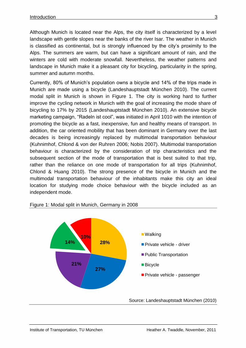
Currently, 80% of Munich‟s population owns a bicycle and 14% of the trips made in
Munich are made using a bicycle (Landeshauptstadt München 2010). The current
modal split in Munich is shown in Figure 1. The city is working hard to further
improve the cycling network in Munich with the goal of increasing the mode share of
bicycling to 17% by 2015 (Landeshauptstadt München 2010). An extensive bicycle
marketing campaign, “Radeln ist cool”, was initiated in April 1010 with the intention of
promoting the bicycle as a fast, inexpensive, fun and healthy means of transport. In
addition, the car oriented mobility that has been dominant in Germany over the last
decades is being increasingly replaced by multimodal transportation behaviour
(Kuhnimhof, Chlond & von der Ruhren 2006; Nobis 2007). Multimodal transportation
behaviour is characterized by the consideration of trip characteristics and the
subsequent section of the mode of transportation that is best suited to that trip,
rather than the reliance on one mode of transportation for all trips (Kuhnimhof,
Chlond & Huang 2010). The strong presence of the bicycle in Munich and the
multimodal transportation behaviour of the inhabitants make this city an ideal
location for studying mode choice behaviour with the bicycle included as an
independent mode.
Figure 1: Modal split in Munich, Germany in 2008
Source: Landeshauptstadt München (2010)
28%
27% 21%
14% 10%
Walking
Private vehicle - driver
Public Transportation
Bicycle
Private vehicle - passenger
Introduction 4
Institute of Transportation, TU München Heather A. Twaddle, November, 2011
Chapter 2 of this thesis provides a detailed overview of previous literature. The first
section of this chapter, Section 2.1 summarizes previous research concerning
bicycle transportation. Section 2.2 gives a brief overview of the theory of discrete
choice analysis. The final section of Chapter 2, Section 2.3 provides a detailed
introduction to stated choice experimental design.
Chapter 3 gives a detailed description of the methodology used in this research
project. The sample recruitment is summarized in Section 3.1, the design of the time-
use-travel diaries is explained in Section 3.2, the means of distribution and collection
for the time-use-travel diaries is outlined in Section 3.3. The coding of the time-use-
travel diaries and the estimation of the attributes of non-selected alternatives is given
in Section 3.4, the design of the stated choice experiment is explained in detail in
Section 3.5, information about the personal questionnaire is included in Section 3.6
and the online distribution of the stated choice experiment and the personal
questionnaire is described in Section 3.6.
The response to the survey (Section 4.1) and the results obtained from the time-use-
travel diaries (Section 4.2) and the stated choice experiment (Section 4.3) are
provided in Chapter 4. A discussion of the project methodology and the results
obtained from the survey follows in Chapter 5. The sample recruitment is discussed
in Section 5.1, the time-use-travel diary in Section 5.2 and the stated choice
experiment in Section 5.3. Chapter 6 provides conclusions derived from the entire
research project.

Literature Review, Bicycle Transportation Research Review 5
Institute of Transportation, TU München Heather A. Twaddle, November, 2011
2. LITERATURE REVIEW
A review of previous research is carried out in three main topic areas; bicycle
transportation, choice modelling and stated choice survey design. A comprehensive
and thorough review of the findings and research methods used in bicycle
transportation research is presented first in Section 2.1. In order to account for the
locality of bicycle transport, the findings from research undertaken in Europe have
been given particular attention. However, because the vast majority of quantitative
bicycle research has been carried out in North America, findings and methods used
in these studies are also presented. A brief presentation of choice modelling
fundamentals is presented in Section 2.2. Because the scope of this research project
focuses on the development of a stated choice survey rather than on a meticulous
review of choice modelling methods, this section only provides an overview of the
basic theory and the development of the multinomial logit (MNL) model. Section 2.3
gives a review of stated choice survey design with particular focus on the theory
behind the methods used in this research project.
2.1. Bicycle Transportation Research Review
Previous research has identified many factors that influence bicycle use. According
to Heinen, van Wee and Maat (2010) in their comprehensive review of bicycle
literature, the factors affecting bicycling for utilitarian purposes can be subdivided into
five groups; the built environment, the natural environment, socio-economic
variables, psychological factors and transportation related factors including cost,
time, effort and safety. These five groups of influencing factors are adopted as a
framework for this research review. The transportation related factors section is
expanded to include destination facilities for cyclists including parking facilities as
well as shower and change rooms. For each section, a small summary of the findings
is given. A table containing a more comprehensive review of the findings of a
selected number of studies is included in Appendix A.
Although a comprehensive overview of the literature is given in this section, particular
emphasis is placed on factors that are responsive to change in policy or
infrastructure provision. The natural environment, for instance, may indeed play a
significant role in the choice to travel by bicycle, but is difficult or impossible to
change to favour bicycle transport. As such, less attention is placed on this group of
factors in the literature review.
Literature Review, Bicycle Transportation Research Review 6
Institute of Transportation, TU München Heather A. Twaddle, November, 2011
2.1.1. Built Environment
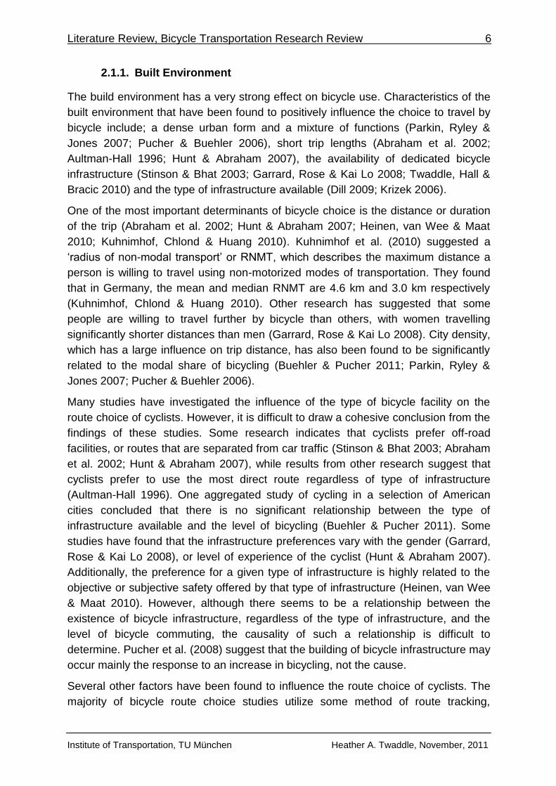
The build environment has a very strong effect on bicycle use. Characteristics of the
built environment that have been found to positively influence the choice to travel by
bicycle include; a dense urban form and a mixture of functions (Parkin, Ryley &
Jones 2007; Pucher & Buehler 2006), short trip lengths (Abraham et al. 2002;
Aultman-Hall 1996; Hunt & Abraham 2007), the availability of dedicated bicycle
infrastructure (Stinson & Bhat 2003; Garrard, Rose & Kai Lo 2008; Twaddle, Hall &
Bracic 2010) and the type of infrastructure available (Dill 2009; Krizek 2006).
One of the most important determinants of bicycle choice is the distance or duration
of the trip (Abraham et al. 2002; Hunt & Abraham 2007; Heinen, van Wee & Maat
2010; Kuhnimhof, Chlond & Huang 2010). Kuhnimhof et al. (2010) suggested a
„radius of non-modal transport‟ or RNMT, which describes the maximum distance a
person is willing to travel using non-motorized modes of transportation. They found
that in Germany, the mean and median RNMT are 4.6 km and 3.0 km respectively
(Kuhnimhof, Chlond & Huang 2010). Other research has suggested that some
people are willing to travel further by bicycle than others, with women travelling
significantly shorter distances than men (Garrard, Rose & Kai Lo 2008). City density,
which has a large influence on trip distance, has also been found to be significantly
related to the modal share of bicycling (Buehler & Pucher 2011; Parkin, Ryley &
Jones 2007; Pucher & Buehler 2006).
Many studies have investigated the influence of the type of bicycle facility on the
route choice of cyclists. However, it is difficult to draw a cohesive conclusion from the
findings of these studies. Some research indicates that cyclists prefer off-road
facilities, or routes that are separated from car traffic (Stinson & Bhat 2003; Abraham
et al. 2002; Hunt & Abraham 2007), while results from other research suggest that
cyclists prefer to use the most direct route regardless of type of infrastructure
(Aultman-Hall 1996). One aggregated study of cycling in a selection of American
cities concluded that there is no significant relationship between the type of
infrastructure available and the level of bicycling (Buehler & Pucher 2011). Some
studies have found that the infrastructure preferences vary with the gender (Garrard,
Rose & Kai Lo 2008), or level of experience of the cyclist (Hunt & Abraham 2007).
Additionally, the preference for a given type of infrastructure is highly related to the
objective or subjective safety offered by that type of infrastructure (Heinen, van Wee
& Maat 2010). However, although there seems to be a relationship between the
existence of bicycle infrastructure, regardless of the type of infrastructure, and the
level of bicycle commuting, the causality of such a relationship is difficult to
determine. Pucher et al. (2008) suggest that the building of bicycle infrastructure may
occur mainly the response to an increase in bicycling, not the cause.
Several other factors have been found to influence the route choice of cyclists. The
majority of bicycle route choice studies utilize some method of route tracking,
Literature Review, Bicycle Transportation Research Review 7
Institute of Transportation, TU München Heather A. Twaddle, November, 2011
generally GIS, and compare the routes travelled by cyclists to non-selected
alternative routes. The characteristics of the selected route are then compared with
the characteristics of the non-selected routes. The findings of such research projects
indicate unanimously that cyclists avoid steep grades (Aultman-Hall 1996; Menghini
et al. 2009). The influence of the number of traffic lights on the selected route was
found to be insignificant in Switzerland (Menghini et al. 2009), while cyclists in
Canada were found to use traffic controls to turn from a street with less traffic to one
with heavier traffic (Aultman-Hall 1996).
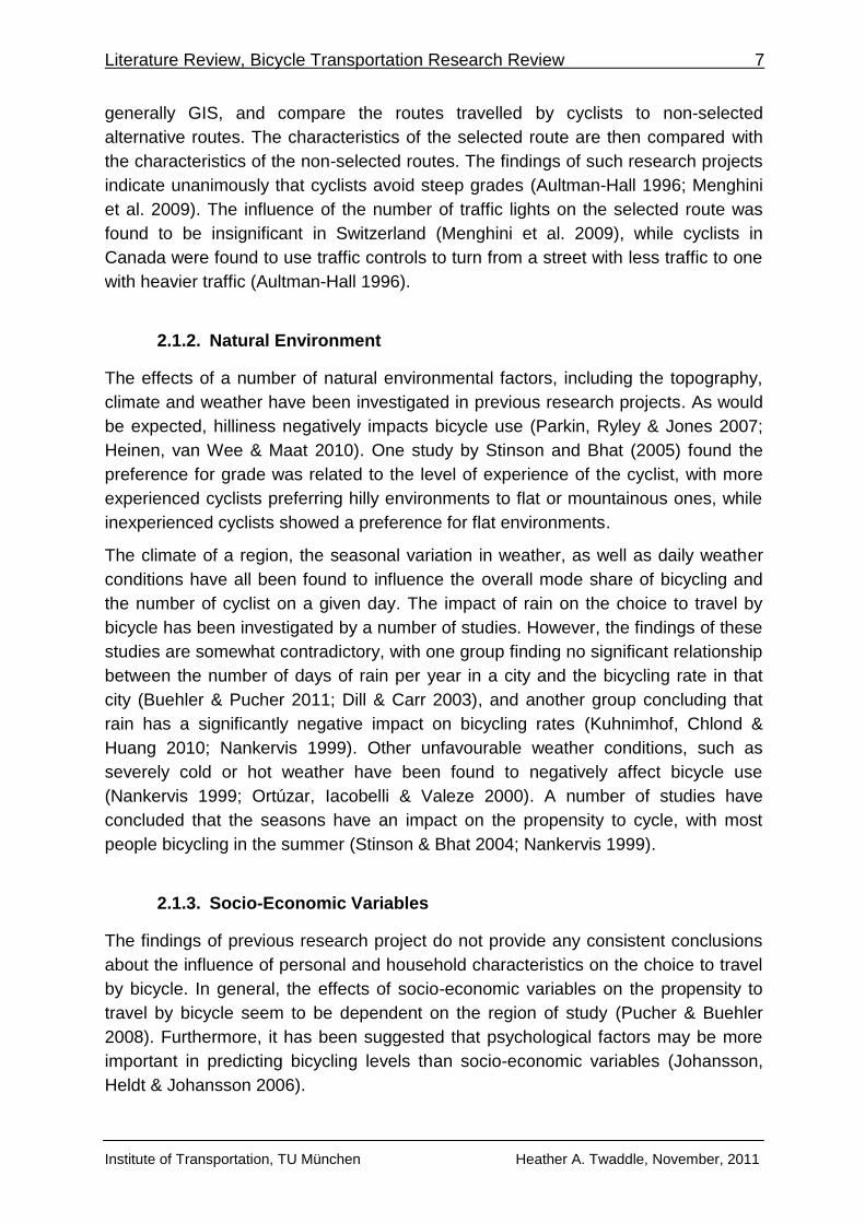
2.1.2. Natural Environment
The effects of a number of natural environmental factors, including the topography,
climate and weather have been investigated in previous research projects. As would
be expected, hilliness negatively impacts bicycle use (Parkin, Ryley & Jones 2007;
Heinen, van Wee & Maat 2010). One study by Stinson and Bhat (2005) found the
preference for grade was related to the level of experience of the cyclist, with more
experienced cyclists preferring hilly environments to flat or mountainous ones, while
inexperienced cyclists showed a preference for flat environments.
The climate of a region, the seasonal variation in weather, as well as daily weather
conditions have all been found to influence the overall mode share of bicycling and
the number of cyclist on a given day. The impact of rain on the choice to travel by
bicycle has been investigated by a number of studies. However, the findings of these
studies are somewhat contradictory, with one group finding no significant relationship
between the number of days of rain per year in a city and the bicycling rate in that
city (Buehler & Pucher 2011; Dill & Carr 2003), and another group concluding that
rain has a significantly negative impact on bicycling rates (Kuhnimhof, Chlond &
Huang 2010; Nankervis 1999). Other unfavourable weather conditions, such as
severely cold or hot weather have been found to negatively affect bicycle use
(Nankervis 1999; Ortúzar, Iacobelli & Valeze 2000). A number of studies have
concluded that the seasons have an impact on the propensity to cycle, with most
people bicycling in the summer (Stinson & Bhat 2004; Nankervis 1999).
2.1.3. Socio-Economic Variables
The findings of previous research project do not provide any consistent conclusions
about the influence of personal and household characteristics on the choice to travel
by bicycle. In general, the effects of socio-economic variables on the propensity to
travel by bicycle seem to be dependent on the region of study (Pucher & Buehler
2008). Furthermore, it has been suggested that psychological factors may be more
important in predicting bicycling levels than socio-economic variables (Johansson,
Heldt & Johansson 2006).
Literature Review, Bicycle Transportation Research Review 8
Institute of Transportation, TU München Heather A. Twaddle, November, 2011
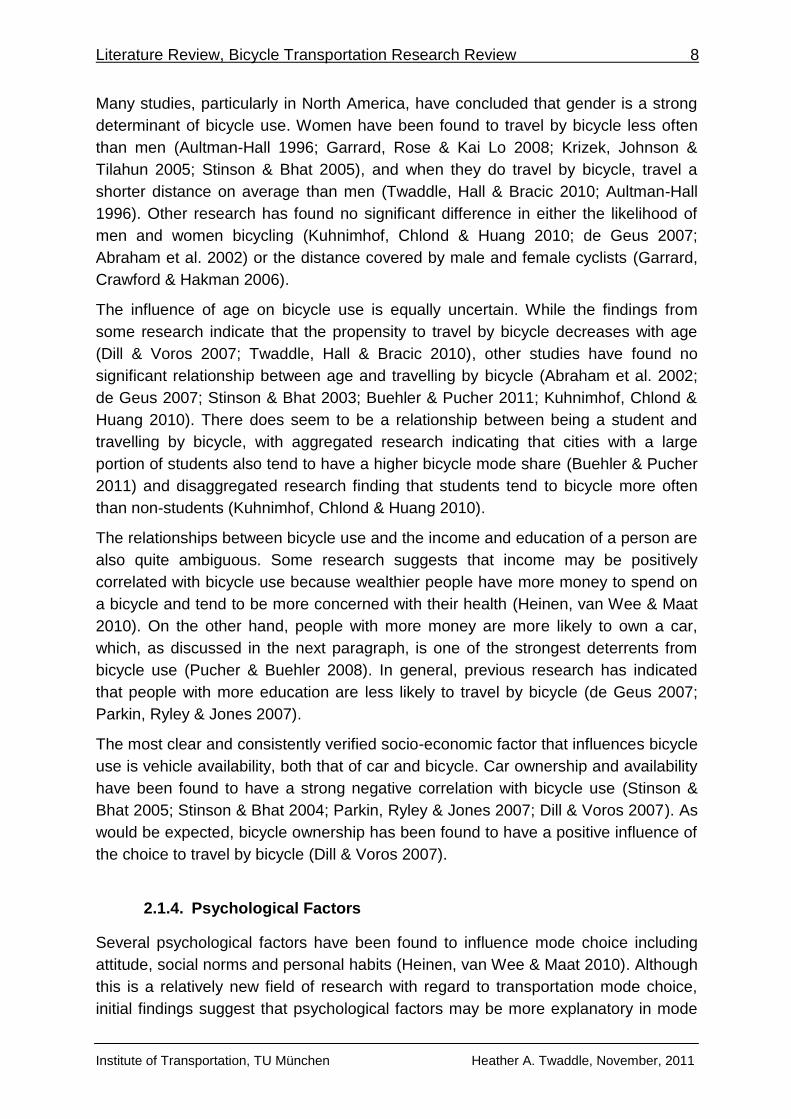
Many studies, particularly in North America, have concluded that gender is a strong
determinant of bicycle use. Women have been found to travel by bicycle less often
than men (Aultman-Hall 1996; Garrard, Rose & Kai Lo 2008; Krizek, Johnson &
Tilahun 2005; Stinson & Bhat 2005), and when they do travel by bicycle, travel a
shorter distance on average than men (Twaddle, Hall & Bracic 2010; Aultman-Hall
1996). Other research has found no significant difference in either the likelihood of
men and women bicycling (Kuhnimhof, Chlond & Huang 2010; de Geus 2007;
Abraham et al. 2002) or the distance covered by male and female cyclists (Garrard,
Crawford & Hakman 2006).
The influence of age on bicycle use is equally uncertain. While the findings from
some research indicate that the propensity to travel by bicycle decreases with age
(Dill & Voros 2007; Twaddle, Hall & Bracic 2010), other studies have found no
significant relationship between age and travelling by bicycle (Abraham et al. 2002;
de Geus 2007; Stinson & Bhat 2003; Buehler & Pucher 2011; Kuhnimhof, Chlond &
Huang 2010). There does seem to be a relationship between being a student and
travelling by bicycle, with aggregated research indicating that cities with a large
portion of students also tend to have a higher bicycle mode share (Buehler & Pucher
2011) and disaggregated research finding that students tend to bicycle more often
than non-students (Kuhnimhof, Chlond & Huang 2010).
The relationships between bicycle use and the income and education of a person are
also quite ambiguous. Some research suggests that income may be positively
correlated with bicycle use because wealthier people have more money to spend on
a bicycle and tend to be more concerned with their health (Heinen, van Wee & Maat
2010). On the other hand, people with more money are more likely to own a car,
which, as discussed in the next paragraph, is one of the strongest deterrents from
bicycle use (Pucher & Buehler 2008). In general, previous research has indicated
that people with more education are less likely to travel by bicycle (de Geus 2007;
Parkin, Ryley & Jones 2007).
The most clear and consistently verified socio-economic factor that influences bicycle
use is vehicle availability, both that of car and bicycle. Car ownership and availability
have been found to have a strong negative correlation with bicycle use (Stinson &
Bhat 2005; Stinson & Bhat 2004; Parkin, Ryley & Jones 2007; Dill & Voros 2007). As
would be expected, bicycle ownership has been found to have a positive influence of
the choice to travel by bicycle (Dill & Voros 2007).
2.1.4. Psychological Factors
Several psychological factors have been found to influence mode choice including
attitude, social norms and personal habits (Heinen, van Wee & Maat 2010). Although
this is a relatively new field of research with regard to transportation mode choice,
initial findings suggest that psychological factors may be more explanatory in mode
Literature Review, Bicycle Transportation Research Review 9
Institute of Transportation, TU München Heather A. Twaddle, November, 2011
selection than socio-economic factors such as gender and age (Johansson, Heldt &
Johansson 2006). This may be particularly true for the choice to bicycle, as socio-
economic variables have been found by many studies to be inadequate predictors of
bicycle use (Kuhnimhof, Chlond & Huang 2010; Abraham et al. 2002; de Geus
2007).
Attitudinal factors such as the preference for convenience, comfort, flexibility and
environmental concern have been found to influence mode choice (Johansson, Heldt
& Johansson 2006), although no work was found that examined the influence of
these attitudinal factors on bicycle use. The attitude of a person toward different
modes of transportation has been found to affect their mode choice (Dill & Voros
2007). Dill and Voros (2007) found that people who are positive about travelling by
bicycle and people who dislike driving a car are more likely to use a bicycle. The
social norms perceived by a person also have a strong influence on their choice to
bicycle or not. Cyclists are significantly more likely than non-cyclists to perceive
social support for bicycling and to have a bicycling partner (de Geus 2007).
The existence of habits has been found to greatly influence a person‟s mode choice.
Although discrete choice modelling is based on the assumption that people use
rational choice when facing a decision (Ben-Akiva & Lerman 1985), research
indicates that people may not consider every factor or alternative when making
repetitive decisions. Instead, they rely on the decision making process that they
employed last time they were required to make the choice (Bamberg & Schmidt
1994). However, because it is generally not possible for a person to meet all their
transportation needs using a bicycle, bicyclists have been found to be multimodal
people who are comfortable evaluating the characteristics of each trip and then
selecting the most suitable mode of transportation (Kuhnimhof, Chlond & Huang
2010).
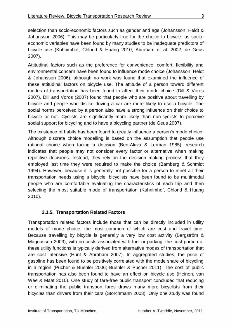
2.1.5. Transportation Related Factors
Transportation related factors include those that can be directly included in utility
models of mode choice, the most common of which are cost and travel time.
Because travelling by bicycle is generally a very low cost activity (Bergström &
Magnussen 2003), with no costs associated with fuel or parking, the cost portion of
these utility functions is typically derived from alternative modes of transportation that
are cost intensive (Hunt & Abraham 2007). In aggregated studies, the price of
gasoline has been found to be positively correlated with the mode share of bicycling
in a region (Pucher & Buehler 2006; Buehler & Pucher 2011). The cost of public
transportation has also been found to have an effect on bicycle use (Heinen, van
Wee & Maat 2010). One study of fare-free public transport concluded that reducing
or eliminating the public transport fares draws many more bicyclists from their
bicycles than drivers from their cars (Storchmann 2003). Only one study was found

Literature Review, Bicycle Transportation Research Review 10
Institute of Transportation, TU München Heather A. Twaddle, November, 2011
that estimated the value of time spent bicycling. Abraham et al. (2002) estimated that
bicyclists in Calgary, Canada value time spent bicycling on a path in a park area at
$4/hour (≈2.9 €/hour) and time spent bicycling on an arterial road at $17/hour (≈12.1
€/hour). In general, research findings have indicated that cyclists are particularly
sensitive to travel time (Abraham et al. 2002; Wardman, Tight & Page 2007;
Kuhnimhof, Chlond & Huang 2010).
2.1.6. Destination Facilities
The provision of safe and secure parking at the destination has been found by
several studies to increase the likelihood of commuting by bicycle (Abraham et al.
2002; Stinson & Bhat 2004). According to Abraham et al. (2007), the most preferred
type of bicycle parking facility are bicycle lockers, followed by bicycle enclosures and
bicycle racks. Many studies also suggest that the value placed on parking facilities by
bicyclists may vary by socio-economic factors and bicycle cost (Abraham et al. 2002;
Hunt & Abraham 2007; Dickinson et al. 2003).
The availability of facilities for cyclists at the destination has been found in some
studies to increase the likelihood of travelling by bicycle. Research done in North
America tends to indicate that the availability of showers and lockers at the
workplace has a small, but significant influence on the attractiveness of bicycling
(Hunt & Abraham 2007; Abraham et al. 2002). However, research done in the United
States found that both the provision of shower and change rooms at the destination
had an insignificant effect on the likelihood to travel by bicycle (Stinson & Bhat 2004).
Only one European study was found in the literature review that examined the effect
of destination showers and change rooms on the likelihood to commute by bicycle. In
Belgium, de Geus (2007) found that the availability of cyclist facilities at the
workplace is associated with bicycle commuting.
2.1.7. Remarks
Although the body of research concerning bicycle transportation is steadily growing,
there is relatively little research that has investigated the bicycle in a mode choice
context. The very low model split of bicycles in most North American cities has made
it difficult to gather sufficient data for bicycle choice modelling (Kuhnimhof, Chlond &
Huang 2010). In Europe, where the bicycling levels make it possible to collect such
data, there are few research projects that quantitatively analyse bicycling. However,
it must be noted that this is a review of the research that is available in English.
There may very well be research done in other European languages that pertain to
bicycle mode choice.
Literature Review, Review of Choice Modelling 11
Institute of Transportation, TU München Heather A. Twaddle, November, 2011
2.2. Review of Choice Modelling
The following section gives a brief overview of the fundamental principles of choice
modelling and remarks regarding the topic.
2.2.1. Overview of Choice Modelling
Discrete choice modelling is an econometric means of predicting the behaviour of
users based on individual choice behaviour theory (Ben-Akiva & Lerman 1985). In
order to predict such behaviour, parameterized utility functions are used. These utility
functions are a combination of independent, observables variables and unknown
weighting parameters. The parameter values are estimated from a sample of
observed choices made by decision makers when faced with a given choice
situation. In discrete choice theory, when making a decision, users are faced with a
set of mutually exclusive and collectively exhaustive alternatives. According to Ben-
Akiva and Lerman, individual choice behaviour is composed of four elements (Ben-
Akiva & Lerman 1985):
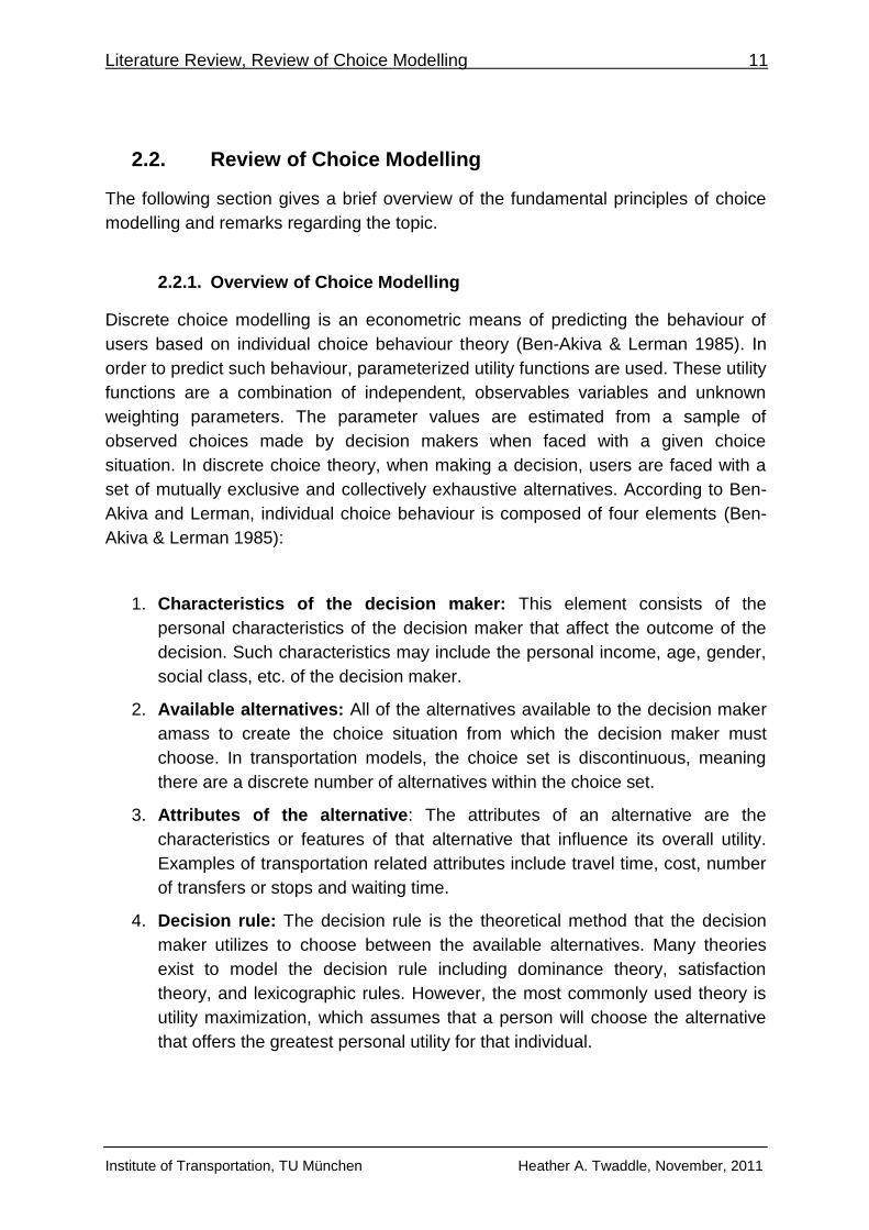
1. Characteristics of the decision maker: This element consists of the
personal characteristics of the decision maker that affect the outcome of the
decision. Such characteristics may include the personal income, age, gender,
social class, etc. of the decision maker.
2. Available alternatives: All of the alternatives available to the decision maker
amass to create the choice situation from which the decision maker must
choose. In transportation models, the choice set is discontinuous, meaning
there are a discrete number of alternatives within the choice set.
3. Attributes of the alternative: The attributes of an alternative are the
characteristics or features of that alternative that influence its overall utility.
Examples of transportation related attributes include travel time, cost, number
of transfers or stops and waiting time.
4. Decision rule: The decision rule is the theoretical method that the decision
maker utilizes to choose between the available alternatives. Many theories
exist to model the decision rule including dominance theory, satisfaction
theory, and lexicographic rules. However, the most commonly used theory is
utility maximization, which assumes that a person will choose the alternative
that offers the greatest personal utility for that individual.
Literature Review, Review of Choice Modelling 12
Institute of Transportation, TU München Heather A. Twaddle, November, 2011
The preceding four elements are based on the assumption that people act rationally
when making a decision. The use of rational behaviour involves employing a
constant and calculated decision process to accomplish short or long term personal
goals. Such behaviour stands in contrast to impulsiveness, in which decisions are
made based on a mood or state of mind at any given time (Ben-Akiva & Lerman
1985).
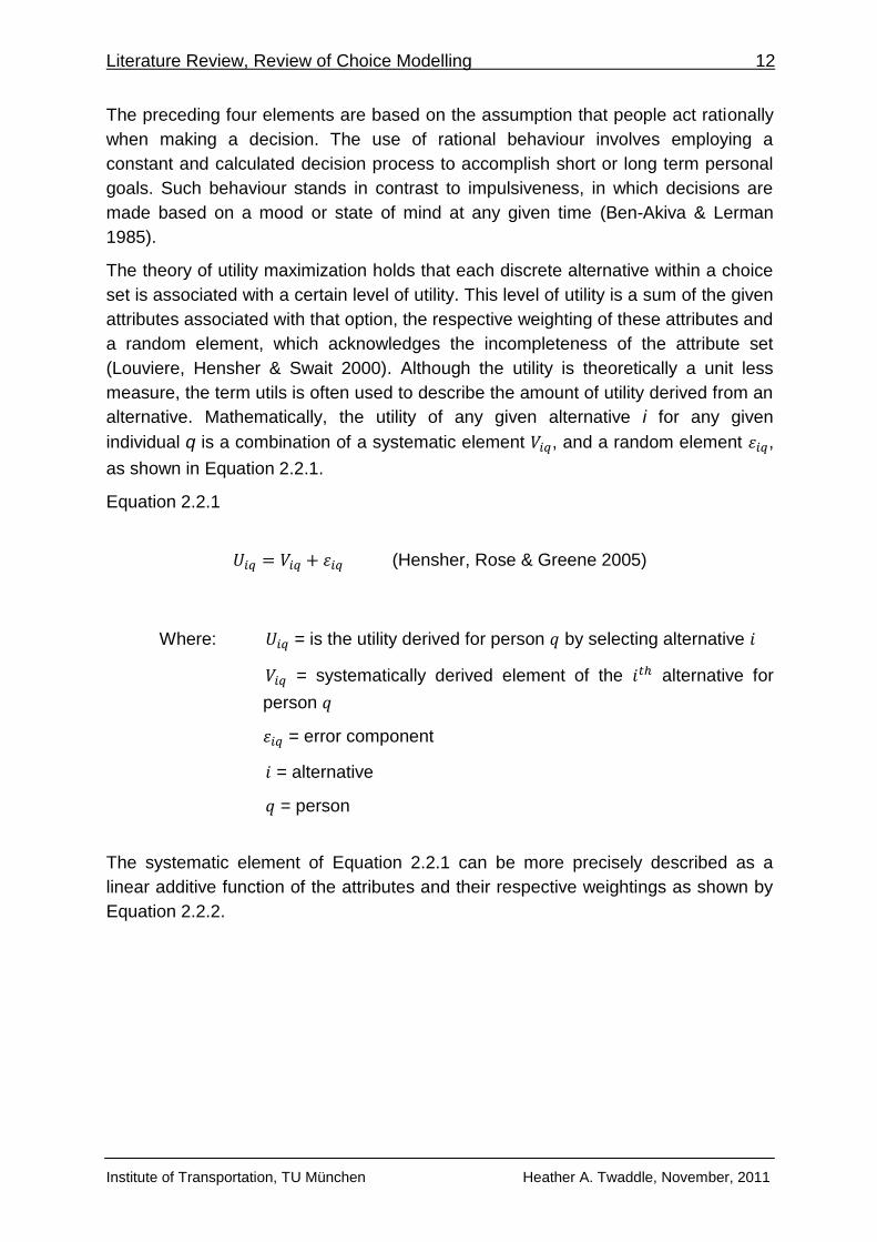
The theory of utility maximization holds that each discrete alternative within a choice
set is associated with a certain level of utility. This level of utility is a sum of the given
attributes associated with that option, the respective weighting of these attributes and
a random element, which acknowledges the incompleteness of the attribute set
(Louviere, Hensher & Swait 2000). Although the utility is theoretically a unit less
measure, the term utils is often used to describe the amount of utility derived from an
alternative. Mathematically, the utility of any given alternative i for any given
individual q is a combination of a systematic element , and a random element ,
as shown in Equation 2.2.1.
Equation 2.2.1
(Hensher, Rose & Greene 2005)
Where: = is the utility derived for person by selecting alternative
= systematically derived element of the alternative for
person
= error component
= alternative
= person
The systematic element of Equation 2.2.1 can be more precisely described as a
linear additive function of the attributes and their respective weightings as shown by
Equation 2.2.2.

Literature Review, Review of Choice Modelling 13
Institute of Transportation, TU München Heather A. Twaddle, November, 2011
Equation 2.2.2
(Hensher, Rose & Greene 2005)
Where: = systematically derived element of the alternative for
person
= alternative specific utility parameter
= independent attribute
= alternative
= attribute associated with alternative
= person
It is assumed that person will choose option A over option B if and only if the utility
of option A is greater than that of option B, or . Expanding this equation
using Equation 2.2.1 yields;
Equation 2.2.3
or;
Equation 2.2.4
(Hensher, Rose & Greene 2005)
The error component of the utility describes the unobservable idiosyncrasies in
taste and preference that differ between individuals (Louviere, Hensher & Swait
2000). Because the error component by definition cannot be estimated, the right
hand part of equation 2.2.4 cannot be calculated. Instead, the probability that the
difference between and is greater than the difference between and is
determined. Although the analyst cannot know the distribution of or , both
distributions are assumed to be related to the choice probability according to a
defined distribution. A random utility model is generated to depict the probability that
a given person will select option A over B based on the assumption that
varies according to some predefined distribution.
In order to operationalize the theory of individual choice behaviour, a number of
axioms have been developed. The most important of these axioms is the
Independence-from-Irrelevant-Alternatives (IIA) axiom, which holds that the ratio of
the probability of choosing one alternative over the probability of choosing the other
is not affected by the presence or absence of other alternatives (Ben-Akiva & Lerman
1985). This axiom implies that all the random elements in the utility functions are
Literature Review, Review of Choice Modelling 14
Institute of Transportation, TU München Heather A. Twaddle, November, 2011
independent across the alternatives and share an identical distribution. One of the
most commonly used distributions, and the distribution that has been used as a basis
for this project, is the extreme value type one (EV1) distribution. By applying the
definition of the EV1 distribution, the basic multinomial logit (MNL) model can be
formed. In this model the probability of selecting alternative is given in Equation
2.2.5.
Equation 2.2.5
(Hensher, Rose & Greene 2005)
Where: = is the probability of selecting alternative
= systematically derived element of alternative
= systematically derived element of alternative
= alternative
= other alternatives
Finally, the β parameters contained in the systematically derived element of the utility
functions are predicted using maximum likelihood estimation (MLE), which uses
statistical methods to determine the population parameters that most often produce
an observed sample.
2.2.2. Remarks
Due to the depth and breadth of the field of discrete choice modelling, it is not
possible to give a detailed review of choice modelling theory in this thesis. The
fundamental equations used for analysis in this research project are provided and
explained, but if the reader is interested in obtaining a full theoretical background on
stated choice methods, the following sources provide a comprehensive overview of
the subject; Ben-Akiva and Lerman 1985, Hensher, Rose and Greene 2005,
Louviere, Hensher and Swait 2000.
Literature Review, Review of Stated Choice Methods 15
Institute of Transportation, TU München Heather A. Twaddle, November, 2011
2.3. Review of Stated Choice Methods
Stated choice experiments are used widely today to determine the independent
influence of various factors on the decisions made by individuals facing a choice
situation (ChoiceMetrics 2011). The ability to predict the individual and aggregated
response to an action is very important in calculating the expected costs and benefits
of that action (Louviere, Hensher & Swait 2000). A brief overview of the types of
choice data available and the methods used to design stated choice experiments are
given in this section.
Historically, there have been two methods for collecting choice data, revealed
preference data sources and stated choice experiments. Revealed preference data is
collected by observing behaviour in the present market. Although such data is highly
reliable and has good face validity, it tends to be expensive and tedious to collect.
There are also several statistical limitations of revealed preference data, including
the inherent relationship between factors and the embodiment of personal and
market constraints (Louviere, Hensher & Swait 2000). Furthermore, the existing
situation often does not provide enough variability in the explanatory variables to gain
a statistically significant understanding of their influence. Conversely, stated choice
experiments are valuable because the behavioural response to a choice situation
that does not yet exist can be inferred (Hensher 1994). In transportation related
studies this can be a very useful quality because the effect of a new policy or
measure can be estimated before it is implemented. Furthermore, in designing a
stated choice experiment, a researcher is able to select and isolate the factors of
influence that are of interest for the research project. Unlike data that is collected
from revealed preference sources, collinearity in the variables can be avoided by
properly designing the stated choice experiment.
The methods used to design statistically robust stated choice experiments have
developed considerably since such experiments were first introduced to the field of
transportation research nearly 20 years ago (Louviere, Hensher & Swait 2000). The
experimental design of any choice experiment involves the planned manipulation of
attribute levels to yield a statistically relevant output.
2.3.1. Selection of the Alternatives, Attributes and Attribute Levels
In creating an experimental design, the researcher must first define the alternatives,
attributes and attribute levels that are to be included in the choice situations. In order
to fulfil the global utility maximizing rule, a universal but finite list of all the existing
alternatives must be compiled. If a complete list is deemed to be too extensive to
create a practical choice experiment, the list of alternatives must be culled (Hensher,
Rose & Greene 2005). The first and most statistically correct method of limiting the
Literature Review, Review of Stated Choice Methods 16
Institute of Transportation, TU München Heather A. Twaddle, November, 2011
number of alternatives presented to each respondent is to randomly select a number
of alternatives from the universal set of alternatives to assign to each participant. A
second approach is for the analyst to make a subjective selection of the significant
alternatives. This approach eliminates all the alternatives that are deemed
insignificant or those that are thought to be only a significant choice for a small
portion of the population. Although this method makes the experimental design
easier to handle and allows the analyst to focus on attributes that are of interest for
the research project, the global utility maximisation assumption is violated.
Once the analyst has determined which alternatives will be included in the choice
situations, the attributes that influence the choice must be considered (Hensher,
Rose & Greene 2005). In selecting the attributes, the analyst must consider which
factors have a significant impact on the preference formation of the decision maker
(Louviere, Hensher & Swait 2000). The attributes included in the choice experiment
may be common among the alternatives, such as departure time, or may be
alternative specific, such as the access time or the number of transfers on a public
transportation journey. There are several factors to consider in defining attributes.
Firstly, it is important that the attribute descriptions are unambiguous (Hensher, Rose
& Greene 2005). The clarity of the attributes and the levels associated with each
attribute are of utmost important in communicating the choice situation to the
decision maker. By including an ambiguous variable, the degree of unobservable
variance in the decision making process of the respondents is likely to increase
(Hensher, Rose & Greene 2005). Furthermore, the applicability of the results is
reduced if attribute ambiguity exists because of a lack of clarity and directness.
According to Hensher, Rose and Green (2005, pp. 106), it is import to be cautious of
cognitive inter-attribute correlations. Although such correlations are not statistical in
nature, a relationship between two variables may exist in the perception of the choice
makers. One example of this is the intrinsic expectation of decisions makers that the
service or quality of a good is related to its price (Louviere, Hensher & Swait 2000).
Another transportation related example of such an inter-attribute correlation could be
the relationship between the comfort of public transportation and the fare. Such
cognitive correlations lead to decision makers using one attribute to make
assumptions about the other features of the option, which reduces the ability of the
analyst to discern the individual influence of the given attribute on the decision
outcome.
The number of attributes that may significantly affect the preference formation of the
decision makers can be quite extensive. However it is beneficial to limit the number
of attributes that are included in a choice experiment for a number of reasons
(Louviere, Hensher & Swait 2000). Firstly, the workload of the respondent increases
in relation to the number of attributes included in the choice situation. This tends to
result in respondent fatigue, which leads to the respondent putting less effort into
evaluating all aspects of the choice situation. As a consequence, the quality of the
Literature Review, Review of Stated Choice Methods 17
Institute of Transportation, TU München Heather A. Twaddle, November, 2011
choice data decreases. Secondly, the experimental design of the choice experiment
increases in size and complexity with the number of attributes and attribute levels
included. By limiting both the number of attributes included in the experiment and the
number of attributes that are used to describe those attributes, the experimental
design can be limited to a more manageable size (ChoiceMetrics 2011).
Finally, the selection of the attribute levels has a large influence on the statistical
power of the stated choice experiment (ChoiceMetrics 2011). The number of attribute
levels included in the experimental design affects the ability of the analyst to
distinguish non-linear relationships between the value of the attribute and the derived
utility (Hensher, Rose & Greene 2005). For example, if the analyst includes only two
levels to describe an attribute, they will have no alternative but to conclude that the
relation between attribute level and derived utility is linear. As more attribute levels
are added to the experimental design, it becomes possible to detect more complex
utility relationships (Hensher, Rose & Greene 2005). However, as mentioned
previously, the size and complexity of the experimental design increases with the
number of included attribute levels. Therefore, the analyst must find a balance
between choosing enough attribute levels to discern the nature of the relationship
between the attribute and the derived utility derived and restraining the size of the
experimental design (ChoiceMetrics 2011).
In addition to setting the number of attribute levels, the maximum and minimum
attribute levels must be carefully considered. The values selected for the maximum
and minimum attribute levels must reflect reality in order to create feasible and
realistic choice situations for the decision makers. On the other hand, it has been
found that models tend to perform poorly for attribute values that are outside of the
range used in the stated choice experiment (Louviere, Hensher & Swait 2000). There
are several methods used for determining which extremes should be used in the
experiment. The first of which is to use revealed preference data to determine
realistic maximum and minimum values (Hensher, Rose & Greene 2005). The
analyst may also choose to use focus groups to determine which attribute levels
seem realistic, and which fall out of the scope of feasibility. Another method
commonly used by analysts is to review the extreme attribute levels used in previous
experiments and to assess the modelling results obtained by using these values.
2.3.2. Experimental Design
The experimental design of a stated choice experiment is the method the analyst
uses to distribute the attribute levels amongst the choice situations and then
distribute these choice situations to the decision makers (survey respondents). The
design of the stated choice experiment has a very large impact on the subsequent
ability of the analyst to draw conclusions about the independent influence of the
selected attributes on the observed choices (ChoiceMetrics 2011). In addition, the
Literature Review, Review of Stated Choice Methods 18
Institute of Transportation, TU München Heather A. Twaddle, November, 2011
experimental design largely affects the statistical power of any models derived from
the data collected in the experiment (Hensher, Rose & Greene 2005). There are
numerous methods that an analyst can employ to design a stated choice experiment;
the most commonly used methods have been summarized in the following sections.
Particular emphasis has been placed on efficient experimental design in this
literature review because there has been an inclination toward this type of design by
experts in recent years. There are many statistical advantages to using efficient
designs, particularly when designing stated choice experiments from revealed
preference data. The full factorial and orthogonal designs will be introduced, but only
the efficient design will be fully explained owing to the fact that an efficient design
has been used in the experiment.
2.3.3. Full Factorial Design
Full factorial designs are the most comprehensive type of choice experiment design
because all of the possible choice situations are considered. Each respondent is
presented with all of the possible choice situations and is asked to select one of the
alternatives. Because all of the possible treatment combinations are considered, it is
statistically possible to evaluate all of the main and interaction effects of the attributes
and attribute levels included in the model (Louviere, Hensher & Swait 2000).
However, the number of treatment situations quickly becomes quite large as the
number of alternatives, attributes and attribute levels increase. In general, the total
number of combinations that are considered in a full factorial design can be
calculated using Equation 2.2.2.1.
Equation 2.2.2.1
(ChoiceMetrics 2011)
Where: = total number of choice situations
= Alternatives
= Attributes of the alternatives
= Levels within the attributes
Because each decision maker is presented with each of the choice situations in a
basic full factorial experimental design, the workload for the respondent becomes
excessively large in all but the smallest experiments (Hensher, Rose & Greene
2005). In addition, as the number of choice situations presented to a respondent
increases, the amount of effort the respondent puts into pragmatically analysing the
Literature Review, Review of Stated Choice Methods 19
Institute of Transportation, TU München Heather A. Twaddle, November, 2011
alternatives and into selecting the most favourable alternative has been found to
decrease (Louviere, Hensher & Swait 2000). One possibility for reducing the number
of choice situations presented to each respondent is to divide the choice situations
among the respondents instead of assigning all situations to all respondents. This
method, however, tend to lead to biased outcomes (ChoiceMetrics 2011). Another
option for limiting the number of treatment situations that are presented to each
decision maker is to systematically select the most important situations for producing
the desired statistical results (ChoiceMetrics 2011). There are a number of methods
that are used for selecting the most important choice situations. The two most
common designs, orthogonal designs and efficient (or optimal) designs are
presented in the following sections.
2.3.4. Fractional Factorial / Orthogonal Design
Orthogonal designs are traditionally the most commonly used form of fractional
factorial stated choice experimental design. According to ChoiceMetrics (2011) an
experimental design is orthogonal if two requirements are satisfied; the attribute
levels are balanced1 and each of the attribute columns in the design is uncorrelated
with the other columns. A problem definition for finding an orthogonal design is given
by ChoiceMetrics (2011, p. 65):
“Given feasible orthogonal coded attribute levels for all and , given a
minimum number of choice situations , determine the smallest balanced
design with such that is
satisfied.”
In creating an orthogonal fractional factorial choice experiment, the analyst will
typically make use of orthogonal coding for the labelling of the attribute levels
because this form of coding makes it less complicated for the analyst to create the
experimental design. Orthogonal coding is achieved when the sum of a column of
attribute levels equals zero. For example, the attribute levels for an attribute with two
levels could be (and conventionally would be) assigned the values 1 and -1. The
attribute levels of an attribute with three levels would be labelled 1, 0 and -1.
Conventionally, only odd numbers are used in orthogonal coding and the number five
is not used
The task of using orthogonal coding to create an orthogonal fractional factorial
design tends to be a tedious process (ChoiceMetrics 2011). A minimum number of
choice situations must be included in order to satisfy the conditions of attribute
1 Attribute balance refers to a condition that all of the attribute levels are included the same number of
times in the experimental design.
Literature Review, Review of Stated Choice Methods 20
Institute of Transportation, TU München Heather A. Twaddle, November, 2011
balance and degrees of freedom2. The minimum number of choice situations that
must be included is six, but depending on the number of alternatives, attributes, and
attribute levels included in the experimental design, the minimum number of choice
situations can be significantly higher (Louviere, Hensher & Swait 2000). In order to
reduce the number of choice situations that are assigned to each survey respondent,
a method known as blocking is used to orthogonally split the design into several
smaller designs (Hensher, Rose & Greene 2005). Each of the smaller designs is no
longer orthogonal within itself, but the sum of the designs maintains orthogonality.
However, recent developments in stated choice experimental design theory, namely
the introduction and improvement of efficient stated choice designs, have highlighted
several shortcomings of the orthogonal fractional factorial method. In practise, it is
atypical to maintain orthogonality within the data set when it is used to create choice
models for several reasons (ChoiceMetrics 2011). Firstly, orthogonality is lost when
data is not collected for any of the choice situations. If blocking is used and one
respondent does not complete their choice task, the orthogonality of the entire data
set is compromised (Louviere, Hensher & Swait 2000). Secondly, the transition from
design codes to orthogonal codes may cause a loss of orthogonality (ChoiceMetrics
2011). For example, if fare attribute is considered for public transportation and the
attribute levels are set at 0.00 €, 0.50 €, 2.00 € and 5.00 €, the subsequent
orthogonal codes -3, -1, 1 and 3 would not accurately represent the quantitative
differences between the levels.
ChoiceMetrics (2011) notes that the use of orthogonal designs is best suited for
analysis using linear models. However, when discrete choice models are used, the
authors suggest that efficient experimental designs may be preferable, even when
limited information is available concerning the β parameters.
2.3.5. Efficient Design
The theory of efficient or optimal experimental designs is presented in this section. It
has been argued in recent literature that if any information exists regarding the β
parameters in the utility functions specified in the model, an efficient experimental
design will always outperform an orthogonal design (ChoiceMetrics 2011). This
applies even if only the sign of the parameters are known or can be assumed
logically.
The underlying principle of an orthogonal fractional factorial method is to create
statistically independent or uncorrelated attributes in the experimental design. While
the construction process of an orthogonal fractional factorial experiment minimizes
2 The degrees of freedom in an experimental design are the number of observations in a sample
minus the number of β parameters that are estimated (Hensher, Rose & Greene 2005).
Literature Review, Review of Stated Choice Methods 21
Institute of Transportation, TU München Heather A. Twaddle, November, 2011
the correlation between the attributes to zero, no effort is made to improve the
statistical efficiency of the design (Hensher, Rose & Greene 2005). In contrast,
efficient designs do not explicitly minimize the correlation between the attributes in
the construction process, although this occurs implicitly in the minimization of the
determinant of the variance-covariance matrix. Instead, they aim at increasing the
statistical efficiency of the experimental design (ChoiceMetrics 2011). The underlying
principle of an efficient design is to minimize the standard error of the parameter
estimates predicted from the stated choice experiment.
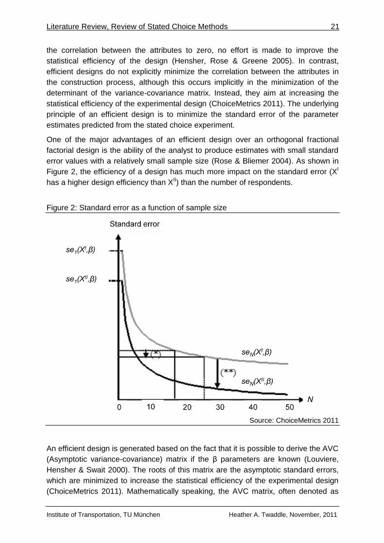
One of the major advantages of an efficient design over an orthogonal fractional
factorial design is the ability of the analyst to produce estimates with small standard
error values with a relatively small sample size (Rose & Bliemer 2004). As shown in
Figure 2, the efficiency of a design has much more impact on the standard error (XI
has a higher design efficiency than XII) than the number of respondents.
Figure 2: Standard error as a function of sample size
Source: ChoiceMetrics 2011
An efficient design is generated based on the fact that it is possible to derive the AVC
(Asymptotic variance-covariance) matrix if the β parameters are known (Louviere,
Hensher & Swait 2000). The roots of this matrix are the asymptotic standard errors,
which are minimized to increase the statistical efficiency of the experimental design
(ChoiceMetrics 2011). Mathematically speaking, the AVC matrix, often denoted as
Literature Review, Review of Stated Choice Methods 22
Institute of Transportation, TU München Heather A. Twaddle, November, 2011
ΩN, is the negative inverse of the Fisher Information Matrix, which itself is the second
derivative of the log-likelihood function. The log-likelihood function of an MNL model
(which is the only type of model that will be analysed in this research project) is given
below.
Equation 2.3.2
(Hensher, Rose & Greene 2005)
Where: = log-likelihood
= the column matrix indicating whether alternative was
selected by respondent in the choice situation
= choice probability from the choice model
= constant
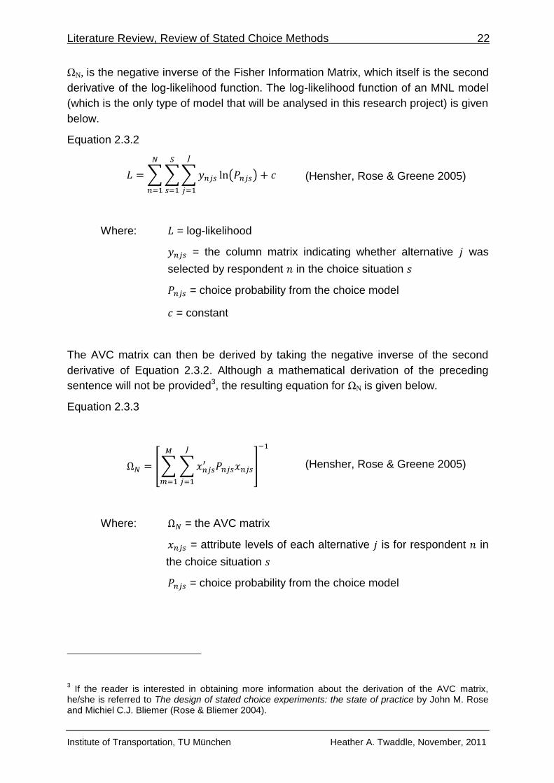
The AVC matrix can then be derived by taking the negative inverse of the second
derivative of Equation 2.3.2. Although a mathematical derivation of the preceding
sentence will not be provided3, the resulting equation for ΩN is given below.
Equation 2.3.3
(Hensher, Rose & Greene 2005)
Where: = the AVC matrix
= attribute levels of each alternative is for respondent in
the choice situation
= choice probability from the choice model
3 If the reader is interested in obtaining more information about the derivation of the AVC matrix,
he/she is referred to The design of stated choice experiments: the state of practice by John M. Rose and Michiel C.J. Bliemer (Rose & Bliemer 2004).
Literature Review, Review of Stated Choice Methods 23
Institute of Transportation, TU München Heather A. Twaddle, November, 2011
The D-error, which is the most commonly used measure of the efficiency of an
efficient stated choice experimental design, is then calculated by taking the
determinant of Equation 2.3.3 (Hensher, Rose & Greene 2005). The aim is to
maximize the efficiency of the design by minimizing the D-error. Although there are
other methods of estimating the efficiency of an experimental design, including the A-
error and S-error measures, only this measure will be reviewed in the scope of this
research project4.
According to ChoiceMetrics (2011), there are three different types of D-error values
that vary depending on the level of information available regarding the β parameters
(known as priors in this case). If no priors information is available, the β parameter
estimates (referred to as in the literature) are assumed to be zero. In this case a
Dz-error is calculated. Alternatively, if there is information available concerning the β
parameters, and this information is deemed to be reasonably accurate, a Dp-error
can be calculated. Lastly, if there is information about the β parameters, but this
information is uncertain, a Db-error can be determined. Using slightly varying
algorithms, all three D-errors can be reduced to produce efficient experimental
designs. As would be assumed, the level of efficiency of the resulting designs varies
according to the quality of the information available concerning the priors.
One of the most common methods of producing an efficient choice experiment is to
use the iterative process depicted in Figure 3. The algorithm is designed to
systematically arrange a set of choice situations from the full factorial design and
calculate the D-error (whichever of the three types of D-error that may be). The
design is then systematically adjusted to reduce the D-error. This loop continues until
a set number of iterations are performed or the analyst discontinues the algorithm.
4 For more information about such error measures please see Stated Choice Methods: Analysis and
Application by Louviere, Hensher and Swait (2000) or the Ngene 1.1 User Manual and Reference Guide (ChoiceMetrics 2011).

Literature Review, Review of Stated Choice Methods 24
Institute of Transportation, TU München Heather A. Twaddle, November, 2011
Figure 3: Flow chart for the modified Federov algorithm
Source: ChoiceMetrics 2011
2.3.6. Building SP Experiments from RP Data
Recent literature has suggested that the realism of a choice situation used in a
choice experiment can be greatly increased by building the alternatives from an
existing situation (Starmer 2000). The use of a reference alternative may produce
more meaningful data at the disaggregated level because the participant is able to
frame the choice task with some existing memory (Rose et al. 2008).
Although the benefits of using a reference situation to build a stated choice
experiment are gaining recognition, the methods employed to integrate revealed
preference data are inconsistent with current techniques of generating SP
experiment (Rose et al. 2008). Firstly, it is difficult to use fixed attribute levels in
stated choice experiments that are built from RP data. This difficulty stems from the
complexity of setting attribute levels that make cognitive sense to all respondents
and reflect the curve of indifference for all respondents. For example, if one
respondent reports a trip that took 2 minutes, another reports 10 minutes, and
another respondent reports a trip that took 30 minutes, it is difficult to set attribute
levels for the attribute trip duration that are appropriate to all three respondents. As
the sample becomes larger, it is increasingly difficult to set suitable attribute levels.

Literature Review, Review of Stated Choice Methods 25
Institute of Transportation, TU München Heather A. Twaddle, November, 2011
There are two common ways of circumventing the problem described previously. The
sample may be divided into separate segments based on the reported value of one
or more variables. It is then possible to use an identical experimental design5 for all
the segments with varied attribute levels that reflect the reported values of the
variables. A second and more commonly used method of avoiding this issue is to
pivot the attribute levels around the reported values using set percentages. This
method is advantageous because the resulting attribute levels will be more akin to
those expected by the decision maker and thus will create more realistic choice
situations (Hensher, Rose & Greene 2005). When designing a pivoted stated choice
experiment, it is important to carefully consider the percentages used to pivot the
observed values as they will have a strong impact on the attribute levels presented to
the respondents and the usability of the resulting data. It must be noted that the
model estimates resulting from this type of choice experiment will be in the form of
percentage changes from a current level (Hensher, Rose & Greene 2005). In other
words, it will not be possible to estimate the effect of an absolute change in a given
factor; only the effect of a percent change will be estimable. Furthermore, it is only
advisable to use the resulting model to predict the effect of percentile changes within
the experimental boundaries.
According to Rose et al. (2008), there are five main methods of implementing pivoted
percentages into a stated choice experimental design. The first of which is to use a
conventional fractional factorial orthogonal design using attribute levels varied by
percentage rather than absolute values. The process of creating such an
experimental design is the same as used for absolute values. However, the efficiency
of such a design is very low because the design is not optimized considering the
actual attribute values presented to the respondents (Rose et al. 2008). The
efficiency, or the D-error value associated with an orthogonal design, was found to
be more than ten times larger than those calculated for the other four design
methods, suggesting that this design will produce larger asymptotic standard errors.
The second method of implementing a stated choice experiment using a reference
scenario is to determine population averages for all the attributes included in the
experimental design and pivot around these values. Although this method was found
to produce a much lower D-error value than the orthogonal design, the reliability of
the parameter estimates for the cost attributes was found to be worse than the
subsequent three methods (Rose et al. 2008).
The third method is an extension of the second method and involves segmenting to
population and determining segment specific averages for the different attributes.
This method produced results similar to those of the second method.
5 It is also possible to create completely different experimental designs for the different segments.
Literature Review, Review of Stated Choice Methods 26
Institute of Transportation, TU München Heather A. Twaddle, November, 2011
The fourth method of building a stated choice experiment from revealed preference
data is to use a two-phase survey instrument. Such an instrument typically collects
RP data from respondents in a paper and pencil survey in a first step and uses this
data to create a stated choice experiment in a second phase. This two-phase method
has been found to be excellent from a statistical standpoint because a data specific
efficient design can be generated by minimizing the values within the AVC matrix
using the same data set used in the model estimation (Rose et al. 2008). However,
such a survey can be difficult to carry out logistically and is subject to drop-outs, or
respondents who take part in the first phase of the survey, but do not complete the
SP experiment (Hensher, Rose & Greene 2005). According to Rose et al. (2008),
although the reliability of the parameter estimates decreases with the percentage of
dropouts, this decrease is only marginal.
The fifth method involves the optimization of the efficiency at the individual level.
Although this method was found to produce the lowest D-error value (Rose et al.
2008), the level of work required to produce such a survey is very large, unless an
automated process is used.
Granting that stated choice experiments built from revealed preference data are
gaining recognition due to their advantages with regards to the decision making
behaviour of the respondents, the methodology used to create such designs is still in
the early phases of development. It is possible to create stated choice experiments
from reference scenarios using some choice experiment building tools such as
Ngene. However, these methods are still somewhat restrictive.
2.3.7. Remarks
The theory of stated choice experiment design is very extensive, and as such, it was
not possible to include all aspects of the theory in this review. If the reader is
interested in learning more about stated choice experimental design he/she is
referred to the text book Applied Choice Analysis: A Primer by David A. Hensher,
John M. Rose and William H. Greene (2005), or Stated Choice Methods: Analysis
and Application by Jordan J. Louviere, David A. Hensher and Joffre D. Swait (2000).
Research Methodology, Sample Recruitment 27
Institute of Transportation, TU München Heather A. Twaddle, November, 2011
3. RESEARCH METHODOLOGY
The methodology used in this research project draws from state-of-the-art practice in
bicycle research, mode choice research and stated choice survey design presented
in Chapter 2. In order to increase the realism of the stated choice experiments for the
respondent, features of an actual trip made by each of the respondents are used to
develop individualized choice situations. The strategy used in this survey to create
personalized choice situations is to implement a two-phase process, where trip
information is gathered from the respondents as a first step, and an efficient stated
choice experiment is created and redistributed to the respondents in a second step.
The following sections explain in detail the way in which the survey logistics and the
experimental design are undertaken. This includes a description of the sample
recruitment, the procedure used to construct, distribute and collect the time-use-
travel diaries, the coding of reported trips and non-selected alternatives and the
method of creating and distributing stated choice experiment and personal
questionnaires.
3.1. Sample Recruitment
When the scope of the survey was set, it was decided that a sample of 50
respondents is required to provide an adequate assessment of the survey design.
No attempt was made to recruit a representative sample of respondents because the
intention of the trial survey is not to collect usable data, but to test the recruitment
process as well as the survey design and methodology. Two survey invitation letters
were written (one in German and one in English) that outlined the intentions of the
research, the requirements of the respondent and participation instructions. Both
versions of the survey invitation letters have been included in Appendix B. Entry in a
draw for one of three 50 € gift certificates to Schuster Sporthaus, a sporting and
outdoor goods shop in Munich, was offered as incentive for participation. The
number of gift certificates was later raised from three to five in an attempt in increase
the attractiveness of participating in the survey. People interested in participating in
the survey were instructed to send an email to [email protected], an email
address created for the administration of this research project. The participants were
instructed to include their mailing address. The time-use-travel diary survey package
was then sent to this mailing address. However, a considerable number of
respondents sent an email confirming their intention to take part in the survey without
stating their mailing address. A response was sent to these people asking explicitly
for their mailing address.
Research Methodology, Sample Recruitment 28
Institute of Transportation, TU München Heather A. Twaddle, November, 2011
Respondents were recruited in two ways. Firstly, because the required number of
participants is relatively small, friends and family members of the people working on
the „Radverkehr heute und morgen‟ project who live in Munich were asked if they
would be willing to take part in the survey. These people were also asked if they had
any roommates, colleagues, friends, etc. who also may be interested in taking part in
the survey. Using this method, 44 people agreed to take part in the survey.
Moreover, seven of the people who agreed to take part in the survey, were also
willing to distribute questionnaires to people at their work or homes and encourage
these people to take part in the survey. A total of 37 additional revealed preference
questionnaires were distributed using this method.
Secondly, survey invitations were mailed to 500 personal addresses in Munich that
were purchased online from Schober Group (www.schober.com). The purchased
addresses did not offer a representative sample, but only included people who have
made their address commercially available in the past. Contact information was only
provided for people over the age of 18 and only for one person per household.
According to the website, contact information is available for 237,643 people in
Munich. However, this recruitment method was not particularly successful; only four
people responding by email to indicate their interest in taking part in the survey,
accounting for a response rate of less than 1%. A small number of survey invitations
did not reach their destination and were returned to the sender.
A survey hotline was available for the entire duration of the survey, from August 22nd
through October 31st, 2011. The intention of the hotline was to answer any questions
that might arise while the respondents were either filling out the time-use-travel diary
or completing the online survey. The hotline was announced first in the information
letter and then online in the introduction to the online survey.
Respondents were originally asked to fill out the time-use-travel diary on any
weekday between August 22nd and September 2nd, 2011, preferably on a Tuesday,
Wednesday or Thursday. This time-frame was later extended, and then eliminated in
order to counteract a low response rate.
Research Methodology, Revealed Preference Survey Design 29
Institute of Transportation, TU München Heather A. Twaddle, November, 2011
3.2. Time-Use-Travel Diary Design
The first phase of the two step research process involved designing a survey
instrument to gather detailed activity and trip information from the respondents.
There are two methods that have been used in past research projects to collect such
information, time-use diaries and travel diaries. Travel diaries are used most
commonly in transportation research, and ask respondents to record information
about each trip made during a pre-set time frame. Collected trip information usually
includes spatial information, such as the origin and destination locations, the purpose
of the trip, the mode used, the time and duration of the trip and the approximate
distance of the trip. Well known travel diaries used for transportation research in
Germany include Mobilität in Deutschland (MiD) and the Deutsche Mobilitätspanel
(MOP). Although travel diaries adequately provide the spatial and trip characteristic
data that is needed for transport research, respondents have been found to omit trips
from the travel diary in an attempt to reduce the work load of the survey (Hubert,
Armoogum & Madre 2008). In contrast, time-use surveys have not been commonly
used in transportation research projects in the past. This type of survey asks
respondents to record all of their daily activities, including trips, in predetermined
time intervals (generally five or ten minutes). Such surveys are thought to be
advantageous because the respondent is not able to reduce the workload of the
survey by omitting trips. However, trips or other activities that are shorter than the
preset recording interval may not be reported in a time-use survey. Furthermore,
time-use surveys used in the past have failed to collect the spatial trip information
that is crucial in transportation modelling.
The time-use-travel diary used in this research project was designed as a combined
time-use-travel diary. This was done in an attempt to draw from the advantages of
both types of surveys while avoiding their respective weaknesses. The diary is based
on the design of time-use surveys, but places a strong focus on both spatial and trip
specific information. The time-use diary instructions and form used in the
„Zeitverwendung in Deutschland 2001/2002‟ (Time use in Germany 2001/2002)
research project (Statistisches Bundesamt Deutschland 2010), were used as a
template for the design of the time-use-travel diary. However, the columns of the
diary that asked for the people who were present during each activity or trip were
removed, and several columns were added to collect travel specific information. For
each activity or trip in the time-use-travel diary respondents are asked to indicate:
the main activity;
the mode of transportation or the address of the activity;
any other additional activity;
the cost of the activity;
the cost of parking;
Research Methodology, Revealed Preference Survey Design 30
Institute of Transportation, TU München Heather A. Twaddle, November, 2011
and the enjoyment of the activity or trip (1-5 Likert Scale).
Several additional columns were added to collect information from people who used
a bicycle for a trip. Bicycle specific information collected in the time-use-travel diary
included:
the type of bicycle parking used (options included public space, bicycle rack,
covered bicycle rack, a bicycle parking house and another parking facility);
the type of infrastructure used for the largest portion of the trip (options
included speed limit 30 km/h zones, bicycle lane on the road, street without a
bicycle lane, bicycle lane on the sidewalk, bicycle path in a green area, a
combined pedestrian and bicycle path and another type of infrastructure);
the availability of showering facilities at the destination;
and the use of showering facilities at the destination if available.
During the design phase of time-use-travel diary, two alternative diaries were
created, a 10-minute interval version, which utilized a preset time interval, and a free
interval version, which allowed respondents the freedom to record the start and end
times of each trip or activity. The free interval version was created in an attempt to
reduce the likelihood of trips being omitted from the diary because they are shorter
than the preset interval. The free interval version of the time-use-travel diary has
been included in Appendix C (German version) and D (English version). The 10-
minute interval version is available on the accompanying CD.
A small qualitative pre-test of the two time-use-travel diaries was carried out on a
convenience sample of seven test respondents. Test respondents were asked to
read the instructions for both prototypes and were shown a filled out example of both
versions. They were then asked which version they would prefer filling out and
whether they would be more likely to omit information on one of the versions. The
test respondents were also asked if they had any general comments or suggestions
about the overall layout of the diary form or the survey instructions. The test
respondents unanimously agreed that they would prefer filling out the free interval
version and indicated that they would not be likely to omit information from either of
the versions. Based on the results of the small pre-test and in an attempt to
maximize the number of survey respondent, it was decided to use the free interval
time-use-travel diary. Several small adjustments were made to the layout of the diary
form and the wording of the instruction text based on the comments and suggestions
of the test respondents.
A space for comments about the survey was provided for the respondents on the last
page of the diary. Respondents were asked to enter any suggestions they may have
for the further development of the survey or indicate any difficulties they had in filling
out the survey in the provided space.

Research Methodology, Time-Use-Travel Diary Distribution and Collection 31
Institute of Transportation, TU München Heather A. Twaddle, November, 2011
3.3. Time-Use-Travel Diary Distribution and Collection
A time-use-travel diary package was sent by mail to each person that emailed their
address to the „Radverkehr heute und morgen‟ email address. Additional time-use-
travel diary packages were distributed by hand by the seven survey participants who
agreed to further distribute the survey. A total of 85 time-use-travel diaries were
distributed either by mail or by hand on Tuesday, August 16th, 2011. In the following
weeks several more people indicated an interest in taking part in the survey, and
subsequently, 12 more survey packages were distributed after the initial delivery
date. Each time-use-travel diary package contained a shortened information letter,
an instruction document containing an example of a correctly completed time-use-
travel diary, a time-use-travel diary form, a short questionnaire sheet and a stamped
and addressed return envelope. Because the survey packages were distributed to
people who had not previously emailed their intention to take part in the survey,
respondents were asked to state their email address and their name on the front of
the survey package, making it possible to distribute the subsequent online survey
link. The documents that were sent to the survey respondents in the time-use-travel
diary package have been included in Appendix C. Distribution of the survey
packages was concluded on Friday September 16th, 2011, after a total of 97 survey
packages were assembled and distributed. Respondents were instructed to insert
the filled out time-use-travel diary, the diary cover page and the questionnaire sheet
into the provided return envelope and mail it back as quickly as possible.

Research Methodology, Coding the Time-Use-Travel Diaries 32
Institute of Transportation, TU München Heather A. Twaddle, November, 2011
3.4. Coding the Time-Use-Travel Diaries and Estimation of Non-Selected Alternatives
All of the trips that were reported in the time-use-travel diaries were coded using
SPSS. A total of 44 variables were created to describe the trips reported in the
diaries and the attributes of the non-selected alternatives. The resulting SPSS file is
available on the accompanying CD (file: RP Dataset.sav).
Several variables were introduced to describe the characteristics of the reporting day
and the respondent. These variables included:
the assigned respondent identification number (1-48);
the reporting date;
the weekday of the reporting date (Monday, Tuesday, Wednesday, etc.);
whether the reporting day was considered normal or unusual;
if the reporting day was unusual, the reason that the day was not normal;
and the weather on the reporting day (overall).
Several additional variables were created to describe the details of each individual
trip made during the reporting day. Data for the trip variables was taken directly from
the time-use-travel diary. These variables included;
the assigned tour identification number6 of the trip;
the assigned trip identification number;
the start address;
the type of start location (e.g. home, work, school, shopping, etc.);
the start time;
the end address;
the type of end locations (e.g. home, work, school, shopping, etc.);
the end time;
the mode used;
if the person used a car,
o the size class of the vehicle,
o the cost of parking at the destination,
o and whether the person was a driver or passenger;
if the person used a bicycle,
o the type of bicycle parking used,
o the type of infrastructure used on the trip (a serious of binary
variables),
6 Tours are defined as a group of trips made by a respondent that start at home, reach one activity or
more, and end back at home.
Research Methodology, Coding the Time-Use-Travel Diaries 33
Institute of Transportation, TU München Heather A. Twaddle, November, 2011
o the availability of showering facilities at the destination,
o and the use of showering facilities at the destination;
the cost of the activity at the destination;
and the enjoyment rating of the journey (1-5 Likert Scale).
Three additional variables were calculated or deduced from the information recorded
in the time-use-travel diaries:
the duration of the trip;
the purpose of the trip;
and the duration of the activity at the destination.
Finally, several variables were added to the dataset that estimated the
characteristics of the non-selected alternatives. Depending on the mode used by the
respondent for the reported trip, a selection of the following variables was estimated:
the distance by car;
the travel time by car;
the distance by bicycle;
the travel time by bicycle;
the access time to public transport by foot;
the travel time by public transport;
the mode of public transport used;
the number of transfers required using public transport;
and the cost of a one way ticket for the trip.
The characteristics of the non-selected alternatives were estimated differently
depending on the mode of transport that was reported by the respondent. The
characteristics of alternative modes of transportation were only estimated for
reported trips that were made by car, public transport or bicycle. Trips that were
made by foot were generally found to be too short for a feasible car or public
transport alternative to exist. Regardless of the mode used for the trip, the travel
distance for the car and bicycle was estimated by entering the origin and destination
addresses into the Google Maps © direction web tool, with the car option selected for
trips made by a car, and the walking option selected for trips made by bicycle. The
walking option was used for bicycle trips to account for the fact that bicycles can
travel through parks and other areas that are not accessible by cars. The rest of the
process varied depending on the mode that was used for the reported trip. Table 1
provides a summary of methods used to estimate the variable values.

Research Methodology, Coding the Time-Use-Travel Diaries 34
Institute of Transportation, TU München Heather A. Twaddle, November, 2011
Table 1: Coding of Alternative Modes of Transportation
Mode Used
Variable Car
Public
Transportation Bicycle
Distance by car Estimated using origin and destination addresses and Google
Maps © directions web tool (with car option selected)
Travel time by car
Value taken as
reported in time-use-
travel dairy
Estimated using origin and destination
addresses and Google Maps © directions
web tool (with car option selected)
Distance by bicycle Estimated using origin and destination addresses and Google
Maps © directions web tool (with walking option selected)
Travel time by bicycle
Estimated using origin and destination
addresses and Google Maps © directions
web tool (with walking option selected) and
Equation 3.4.1
Value taken as
reported in time-use-
travel dairy
PuT Access time Estimated using
origin and
destination
addresses, trip start
time and the MVV
online trip planning
tool
Value taken from
time-use-travel diary
when available and
estimated using
origin and
destination
addresses, trip start
time and the MVV
online trip planning
tool when not
available
Estimated using
origin and
destination
addresses, trip start
time and the MVV
online trip planning
tool
PuT Travel time
PuT Mode
PuT Transfers
PuT Fare
For respondents who used either a car or public transportation for their reported trip,
the travel time for the bicycle alternative was calculated using the following equation:
Equation 3.4.1
Where was estimated using Google Maps © (km)
= 1.12
= 11.78 km/h
Research Methodology, Coding the Time-Use-Travel Diaries 35
Institute of Transportation, TU München Heather A. Twaddle, November, 2011
The detour factor was adopted from the results of a GPS tracking research project
done in Guelph, Canada (Aultman-Hall 1996). Aultman-Hall found that the average
cyclist rode 3.7 km on a one-way bicycle commute, and this distance was an
average of 0.4 km longer than the shortest possible route. Therefore:
The mean speed factor was taken from another GPS tracking research
project that took place in Zurich, Switzerland (Menghini et al. 2009). This speed
represents the average bicycling speed by a person over a one week observation
period. The average speed includes any time stopped during the trip. This study also
compared the trip distance of the selected route to alternative routes, but did not
specifically compare the selected route to the shortest possible route.

Research Methodology, Stated Choice Survey Design 36
Institute of Transportation, TU München Heather A. Twaddle, November, 2011
3.5. Stated Choice Survey Design
A stated choice experiment was designed to estimate the effects of various bicycle
transportation factors and the characteristics of alternative modes of transportation
on mode choice. The data collected in the time-use-travel dairies was incorporated
into the stated choice experimental design to create a realistic choice situation for
each survey participant. The experimental design of the choice experiment was
created using Ngene, a software that is distributed by ChoiceMetrics (www.choice-
metrics.com). The procedure for setting up a choice experiment suggested by
Hensher, Rose and Greene (2005, p 100-156) was used as a guideline for
generating the experimental design used for this choice experiment. The following
section describes the alternatives, attributes and attribute levels that were selected
for assessment and provides an explanation for why such variables were included.
The following sections explain the experimental design used for the stated choice
survey and the rationalization behind the selected methods.
3.5.1. Relevant Alternatives, Attributes and Attribute Levels
As described in Section 2.3, a universal but finite list of all the existing alternatives
must be compiled in order to fulfil the global utility maximizing rule. However, if the
complete list is deemed to be too large to create a practical choice experiment, the
list of alternatives must be culled (Hensher, Rose & Greene 2005). Because the list
of modes of transportation that could be used in Munich is quite long, and includes at
least 20 alternatives, it was necessary to use subjective judgement to select the
most significant alternatives to include in the choice experiment. It was decided to
include three transportation mode alternatives in the choice experiment, the car, an
all encompassing public transportation alternative including the bus, tram, U-Bahn
and S-Bahn, and the bicycle. It was decided not to include walking as an alternative
in the choice situation, even though trips by foot account for 28% of the trips made in
Munich (Landeshauptstadt München 2010). This alternative was omitted because a
distance that is comfortably covered by foot is typically much shorter than that
covered by public transportation, private car or bicycle. In the estimation of the
characteristics of the alternative modes of transportation for the trips reported in the
time-use-trip diaries, it was concluded that the majority of the trips made by foot did
not have a possible public transportation alternative7. Moreover, in many cases, the
estimated travel time for driving was greater than the walk time reported in the travel
diary due to restricted one-way streets. Similarly, the walking alternatives for trips
7 In such cases the MVV trip planning web tool suggested a walking route.
Research Methodology, Stated Choice Survey Design 37
Institute of Transportation, TU München Heather A. Twaddle, November, 2011
made by a public transport mode or by car generally did not have a feasible walking
alternative. However, as this omission is in violation of the global maximizing
condition, some explanatory power of the model is lost.
Once the alternatives to be included in the choice experiment were decided upon, it
was necessary to determine which attributes should be included to describe each of
the alternatives. Although it may have been possible to include common attributes to
describe some or all of the attributes, it was decided to use only alternative specific
attributes in this trial experimental design. This approach was chosen in order to be
able to assess the suitability of the attributes and the attribute levels selected for
each alternative autonomously. However, it would be difficult to create common
attributes for most of the attributes included for three reasons. Firstly, a number of
the attributes only pertained to one alternative, an example of which is the
percentage of dedicated bicycle infrastructure available on the trip. Clearly this
attribute was only relevant for explaining the bicycle option and not the car or public
transport alternatives. Secondly, as found in many previous mode choice
experiments, the influence of similar attributes on the total utility of different modes
tends to be different. For example, travel time was included as a factor in all three
alternatives; however, previous research has indicated that the β parameters differ
depending on the mode. For instance, the travelling by bicycle has been found to be
more onerous per minute than time spent driving a car or riding public transport
(Heinen, van Wee & Maat 2010). In order to be able to calculate the β parameters
individually for the three alternatives, it was decided to use alternative specific travel
time attributes. Finally, the levels associated with a common attribute may vary for
different alternatives, making it necessary to create individual attributes. An example
of this can be made by once again referring to travel time. Depending on the trip
characteristics, the travel time by bicycle, car and public transportation tend to be
quite different. However, because this experimental design makes use of revealed
preference data and attribute levels that are pivoted around a reported value, it may
be possible to use common attribute levels for the different alternatives. As stated
previously, this was not done in this experiment in order to be able to analyse the
attributes and attribute levels independently.
In an attempt to make the experimental design more manageable, efficient and
balanced, it was decided to include three attributes for each of the alternatives. Each
of the attributes was described by two, three or six levels. The attribute levels were
adopted from previous research projects that yielded results with high validity. As
discussed in Section 2.3, the attribute levels should be selected in such a way that
they reflect the estimation of the indifference curve. If the attribute levels are
correctly selected, the variation of the attribute levels in the different choice situations
will marginally influence the decision of the respondent. The attributes organized by
alternative as well as the selected attribute levels will be presented in the next
sections along with a justification for their inclusion.
Research Methodology, Stated Choice Survey Design 38
Institute of Transportation, TU München Heather A. Twaddle, November, 2011
Car
There is a considerable amount of research available that has analysed the influence
of various car attributes on mode choice (Vrtic et al. 2009; Ortúzar, Iacobelli &
Valeze 2000; Bamberg & Schmidt 1994). In the literature review section of the
report, the findings from mode choice studies that included the bicycle have been
presented. The experimental design of these studies, along with the statistical output
and validity of the resulting models, has been closely examined in an attempt to
select the most relevant attributes. The attribute levels used in these studied have
also been used as a guideline for those used in this choice experiment.
Car Travel Time
The vast majority of the mode choice studies that were reviewed included travel time
as an attribute describing all of the modes included in the experiment. As expected,
the results of mode choice stated choice experiments indicate that the travel time β
parameter was both significant and relatively large in absolute value (König &
Axhausen 2002; Ortúzar, Iacobelli & Valeze 2000; Vrtic et al. 2009). Furthermore,
the travel time by car is an attribute that is responsive to policy change. Various push
measures aim at extending the car travel time by reducing speed limits, introducing
traffic-calming measures and closing off certain roads for, and hence decrease the
utility of the car option.
The car travel time attribute was integrated into the stated choice experiment as a
pivoted attribute. The absolute value attribute levels could not be used because of
the wide range of car travel times included in the experiment. The car travel times
reported by the respondents or estimated using Google maps (© Google), were used
as a reference attribute level. The pivoting values were adopted from Vrtic et al.
2009, who used a similar attribute in their mode choice analysis and produced a
robust model from their results. The pivoted attribute levels included for the car travel
time attribute were -10%, 0% (reference scenario) and +25%.
Parking Fee
The decision to include the cost of parking as a separate attribute was made based
on several pieces of information. Two mode choice studies were found in the
research review that included parking fees, Vrtic et al. (2009) and Ortuzar, Iacobelli
and Valeze (2000), both found the independent influence of a parking fee to be
significant and relatively large. Vrtic et al. (2009) found that the absolute value of the
parking fee β parameter was more than 2.5 times greater than that of the fuel cost
component. Secondly, parking control is one of the most commonly used push
measures, or measures that encourage people to use alternative modes of
transportation rather than driving (or riding as a passenger) in a private car. The
introduction of parking fees or the increase in the cost of parking are some of the
quickest and simplest means of controlling parking and supporting alternative modes
of transportation such as the bicycle. Because this attribute is so responsive to policy
Research Methodology, Stated Choice Survey Design 39
Institute of Transportation, TU München Heather A. Twaddle, November, 2011
change, the independent influence of the parking fee on the mode choice decision
was of particular interest.
The parking fee attribute was originally intended to be included as a pivoted attribute
which used the parking fee reported in the time-use-travel diary as a base for the
stated choice experiment. If the respondent did not use a car for their trip, the intent
was to use the typical Munich parking rate of 0.50 € per 12 minutes for parking in the
city centre, and the duration of their activity as reported in the time-use-travel diary to
estimate a parking fee. However, the majority of the respondents who did use a car
for one of their reported trips did not indicate a parking fee. Additionally, the long
duration of many of the reported activities made it unfeasible to use a parking fee
rate of 0.50 € per 12 minutes. If a person reported travelling to work, where they
stayed for eight hours, the resulting parking fee of 20.00 € was deemed to be too
dominating to include in the stated choice experiment. In light of these obstacles, it
was decided to use fixed absolute values for the parking fee attribute levels. The
attributes used were based loosely on those used in two parking studies, one done
in Karlsruhe, Germany and the other in England (Axhausen & Polak 1991). The
attribute levels were also questioned in the small pre-test of the stated choice
experiment to ensure that they did not dominate the decision. The attribute levels
used were 0.00 €, 2.00 € and 5.00 €.
All Inclusive Travel Costs
The total trip cost was included in the experimental design to assess its validity as an
explanatory attribute. In the mode choice literature that was reviewed, those that
included gas price used either an estimated gas cost per km (Vrtic et al. 2009) or per
litre/gallon (Buehler & Pucher 2011), or used an estimated total fuel cost for the trip
(Ortúzar, Iacobelli & Valeze 2000). Although Vrtic et al. (2009) found that the
influence of the fuel cost was significant; the absolute value of this influence was
relatively small. Ortúzar, Iacobelli & Valeze (2000) included the fuel cost in the stated
choice experiment, but the model that was subsequently estimated incorporated a
direct cost attribute, which included parking cost and fuel cost. Although the absolute
value of this parameter was relatively large, the t-ratio hovered near the 5%
significance boundary. These results suggest that the influence of gas price alone on
the decision outcome is modest and in some cases barely significantly relevant. In
addition, the gas price alone does not represent the entire cost imposed on a driver
(or passenger) for using a car.
Furthermore, because trips shorter than 4.6 km were selected with first priority, the
total gas price of any given trip was minuscule8 in comparison to other cost factors
(parking and public transportation fare). During a small pre-trial of the stated choice
8 e.g. 4.6 km * 0.05 €/km = 0.23 €
Research Methodology, Stated Choice Survey Design 40
Institute of Transportation, TU München Heather A. Twaddle, November, 2011
experiment, the convenience sample of respondents indicated verbally that the small
fuel cost variable did not have any influence on their decision.
For these reasons, it was decided to include an all inclusive travel cost attribute,
which includes the depreciation per kilometre, the fuel cost, fixed costs associated
with car ownership including insurance and tax, and variable costs including
maintenance and repair. The value used as the reference point was calculated from
a report prepared by the Allgemeiner Deutscher Automobil-Club e.V. (2011), which
gives the average all inclusive driving cost of over 1500 vehicle models. The median
value given in the report, 0.53 €/km, was calculated and used as the base line value
for the stated choice experiment.
The all inclusive travel cost attribute was included with pivoted attribute levels. The
attribute levels used were adopted from Vrtic et al. (2009), even though the attribute
that was included in their stated choice experiment concerned fuel cost and not an
all-inclusive cost. The attribute levels included are -5% (or 0.50 €/km), 0% (or 0.53
€/km – reference scenario) and 40% (or 0.74 €/km). However, because the attribute
levels are pivoted using percentages rather than absolute values, it is assumed that
the levels are roughly applicable to this new attribute as well. As no previous
literature was found that included this attribute, it is particularly important to assess
its independent influence and the suitability of the pivoted attribute levels.
Public Transportation
Many studies have investigated the influence of various public transportation related
attributes on the decision outcome (Buehler & Pucher 2011; Johansson, Heldt &
Johansson 2006; Kuhnimhof, Chlond & Huang 2010; König & Axhausen 2002; Vrtic
et al. 2009). The attributes that are considered in these studies are wide ranging and
include, travel time, access time, total wait time, number of transfers, headways or
frequency of service, reliability of service, comfort, fare, and various other factors.
Due to the sheer number of attributes that have been investigated concerning public
transportation, it was difficult to discern the most influential attributes in a mode
choice context. However, because the number of attributes and attribute levels
included in a survey design quickly increase the survey complexity and data
requirements, subjective decisions were made as to which attributes were the most
relevant for this research project. The following sections describe the attributes that
were selected and explain how these attributes were implemented in the
experimental design.
Total Access Time and Total Ride Time
The total travel time of a public transportation trip is composed of an access time, a
wait time, a riding time, a transfer wait time (which is a sub-component wait time),
and an egress time. Previous research has indicated that the β parameters of these
Research Methodology, Stated Choice Survey Design 41
Institute of Transportation, TU München Heather A. Twaddle, November, 2011
different segments of total public transportation time are different, or in other words,
passengers tend to value the different components of a transit ride differently
(Johansson, Heldt & Johansson 2006; König & Axhausen 2002; Ortúzar 2000; Vrtic
et al. 2009; Vuchic 2005). In this experiment, it was decided to use two time
components to describe the trip duration, the total access time, which is the sum of
the access and egress time, and the ride time, which includes the ride time and
transfer wait time. The wait time at the first station was neglected because it was
assumed that the traveller could use the scheduling system provided by the transit
service to avoid significant wait times. When considering wait time, the frequency (or
headway) of service would have been a better attribute to examine because this
attribute actually affects the travellers‟ ability to reach their destination at the desired
time. However, this attribute was also disregarded for this experiment because of the
relatively high frequency of public transportation service in Munich9.
The access time was selected because it has been found to have a strong and
significant influence on mode choice (Vrtic et al. 2009) and a very important predictor
of public transportation use (Park & Kang 2008; Hossain, Hunt & Wirasinghe 2010).
Kumnimhof, Chlond and Huang (2010) pointed out that for some trip purposes
(particularly commuting) public transportation is the strongest competitor to the
bicycle within the radius of non-motorized travel, particularly when a stop is very near
to the home. Although the access time is not particularly responsive to short term
policy measures, access time was included as an attribute because of its strong
influence on public transportation use, particularly within the radius of non-motorized
transport. Stringent maximum accessibility distances, or the distance from a
household to the nearest public transportation stop, are enforced in Germany. These
circumstances could have a limiting effect on the significance of this attribute in this
study. The access time attribute levels were pivoted around a reference value by -
15%, 0% (reference scenario) and +30%. The reference value was either taken from
the time-use-travel diary (if reported) or estimated using the trip planner provided by
the MVV.
The public transportation ride time, including transfer time if necessary, was
incorporated as the second component of the public transportation travel time.
Although this attribute has been found to have a lower influence per minute than the
access or wait time (Park & Kang 2008; Vrtic et al. 2009; Hossain, Hunt &
Wirasinghe 2010), it still has a substantial impact on the utility of a public
transportation trip, partially due to the fact that the ride time is typically the longest
portion of the ride (Vuchic 2005). The public transportation ride time is also more
9 The buses, trams and U-Bahn in Munich typically run with a 5- or 10-minute headway during
daytime hours and a 20-minute or 1-hour headways in the late evening and early morning. The S-Bahn generally has a 10- or 20-minute headway in the outskirts of Munich but is coordinated to offer roughly 5-minute headways within the city.
Research Methodology, Stated Choice Survey Design 42
Institute of Transportation, TU München Heather A. Twaddle, November, 2011
responsive to change in policy or operation than the other components. The attribute
levels for ride time were pivoted around a reference value by -20%, 0% (reference
scenario) and +10%. In order to provide a general idea of the total trip time, the
access time and ride time were summed and displayed in a separate row in the
stated choice experiment questions that were given to the respondents.
Fare
The third attribute included for the public transportation alternative was the one-way
fare. Along with travel time, the cost associated with a transportation mode, or fare in
the case of public transportation, has been found to be the most influential factor on
mode choice (Ahern & Tapley 2008; Vuchic 2005; Ortúzar 2000). Public
transportation fare may have a particularly strong influence on the choice to travel by
bicycle. Storchmann (2003) found that in the few cases where fare-free public
transportation service was introduced in European cities, the largest portion of new
passegners attracted to public transport were previously cyclists and pedestrians,
even though the fare-free concept has typically been introduced to reduce car traffic.
Additionally, the public transportation fare is one of the most responsive attributes to
short term policy measures. Because of this responsiveness, the influence of this
attribute is of particular interest to analysts. The fare level for the public
transportation alternative was pivoted around a reference value by -30%, 0%
(reference scenario) and +20%. These levels were adopted from a study done by
Vrtic et al. (2009). The reference value was taken as the cost of a single journey
ticket from the MVV, either for one or two zones depending on the origin and
destination of the reported trip.
Bicycle
The attributes included for the bicycle alternative were considerably more difficult to
decide upon than those for the other two alternatives. This difficulty stemmed
partially from the fact that very few stated choice experiments have been carried out
that investigate bicycle use in a mode choice context. A number of studies involving
stated choice experiments have been carried out to examine bicycle route choice
and frequency of bicycle use. However it is not clear if the attributes included in
these experiments would also be relevant for bicycle mode choice. One study was
found that did examine bicycling in a mode choice context in Chile (Ortúzar, Iacobelli
& Valeze 2000). However, the applicability of the results of this study is limited
because of the differences in transportation behaviour in Europe and South America.
Nevertheless, many of the methods used in that study were used as a guideline for
the integration of a bicycle alterative in a mode choice stated choice experiment. The
following sections outline the attributes that were selected to describe the bicycle
alternative in the choice situation.
Research Methodology, Stated Choice Survey Design 43
Institute of Transportation, TU München Heather A. Twaddle, November, 2011
Bicycle Travel Time
The travel time by bicycle was included in the experimental design because travel
time for all modes has been found in many studies to have a significant influence on
the decision outcome (Vrtic et al. 2009; König & Axhausen 2002; Ortúzar, Iacobelli &
Valeze 2000). Bicycle travel time in particular was found to have a strong and
significant effect on the choice to bicycle (either route or frequency) in studies that
investigated bicycle behaviour (Abraham et al. 2002; Aultman-Hall 1996; Hunt &
Abraham 2007; Krizek 2006; Menghini et al. 2009; Stinson & Bhat 2005; Stinson &
Bhat 2003; Tilahun 2005).
In previous studies involving bicycle travel time, the travel time was deemed to be
fixed or only variable based on how strenuously the cyclist chose to ride. However, it
is argued here that the bicycle travel time is responsive to policy measures.
Measures such as coordinating traffic lights specifically for bicycle traffic, opening
one way streets for contra flow bicycle traffic and giving bicycles the right of way on
certain streets can greatly reduce the travel time for bicyclists without asking them to
put more energy into their trip.
This attribute was implemented in the experimental design as a pivoted attribute.
The reference level (0%) was either taken from the time-use-travel diary or
calculated using an assumed average speed of 11.78 km/h (see Section 3.4 for
derivation of this speed) and a trip distance estimated using Google maps (©
Google). Because no previous work was found that included a changing bicycle
travel time in the mode choice stated choice experiment, the pivoting percentage
levels were loosely based off of those used for the car and public travel times. These
levels were, -15%, 0% and +15%.
Percentage of Dedicated Bicycle Infrastructure on the Trip
The preference of bicyclists concerning the type of infrastructure used for their
bicycle journey has been included in many of the bicycle route choice and frequency
stated choice experiments in the past. Overall, the findings of these studies indicate
that the availability of dedicated bicycle infrastructure is important in selecting a
bicycle route. However, beyond this general conclusion, the findings are mixed
concerning which type of infrastructure cyclists prefer, whether it is bicycle lanes on
sidewalks, separated bicycle lanes, bicycle paths in green areas, traffic calmed
streets, streets with no parking permitted, etc..
As dedicated bicycle infrastructure was found to have a significant influence on
bicycle choices it was decided to include this attribute in this experimental design.
However, because of the mixed findings concerning more detailed subdivisions of
dedicated bicycle infrastructure, it was decided to use this attribute in its general
form. Bicycle infrastructure was not included as an attribute in the bicycle inclusive
mode choice study done by Ortuzar, Iacobelli & Valeze (2000). In their experiment,
Hunt and Abraham (2001) used a uniform distribution of travel times between a set
Research Methodology, Stated Choice Survey Design 44
Institute of Transportation, TU München Heather A. Twaddle, November, 2011
maximum and minimum and assigned respondnents a combined trip with two types
of infrastructure, each described by a randomly selected travel time. This method
was adapted for this study, but because the total travel time was already decided,
the percentage of the trip spent on bicycle infrastructure was used as a tool to derive
the time spent on infrastructure dedicated to bicycle use. The percentages of
dedicated bicycle infrastrure that were included in the experimental design were 0%,
20%, 40%, 60%, 80% and 100%. In order to make this attribute clear to the
respondents, the percentage of dedicated bicycle infrastructure was converted to
time spent on dedicated infractucture and time spent riding in mixed traffic.
Attribute ambiguity was thought to be a potential problem for respondents in using
this attribute to shape their decision. In order to provide the respondents with an idea
of what was meant by dedicated bicycle infrastructure, various pictures of different
infrastructure types were provided in a special information page available on the
stated choice experiment (accessible to the respondents by clicking on the button
positioned under the bicycle alternative description).
Availability of Secure Parking at the Destination
The availability of secure parking at the destination has been found to have a
significant impact on bicycle use by several studies in North America (Abraham et al.
2002; Hunt & Abraham 2007; Stinson & Bhat 2003). However, no research known to
the author has been done in Europe to confirm if secure parking is also an important
consideration for European cyclists. This attribute was modelled after one used in
the research project done by Hunt and Abraham (2001) in Edmonton, Canada. A
binary attribute was created (No secure parking = 0, secure parking = 1) and
implemented into the survey design. As with dedicated bicycle infrastructure,
attribute ambiguity was thought to be a potential problem for the secure parking
attribute. As reported by Hunt and Abraham (2001) some of the respondents may
have seen the attribute level „no secure parking‟ as unrealistic because cyclists can
almost always lock their bicycle to a fence or pole at their destination. In order to
improve upon this point, a definition of secure parking was provided for the
respondents (accessed by clicking on the button positioned under the bicycle
alternative description). If no secure parking was provided, respondents were
advised that they would have to park their bicycle in public space wherever possible.
Attributes Not Included
It was originally intended to investigate the influence of the availability of showers
and lockers at the destination on the likelihood to travel by bicycle. However, in the
revealed preference section of the research, it was found that only very few of the
respondents indicated using a shower or change facility at their destination.
Furthermore, the availability of showers and change rooms is typically only
applicable to work trips. Because all trip purposes were included in the experiment, it

Research Methodology, Stated Choice Survey Design 45
Institute of Transportation, TU München Heather A. Twaddle, November, 2011
was not logical to include the availability of showers in the choice experiment. For
this reason, and in an effort to reduce the number of attributes included in the stated
choice experiment, it was decided to exclude the shower and change room attribute.
Summary of Attribute and Attribute Levels
Table 2 provides a summary of the attributes and attribute levels that were described
in the previous sections. The attribute levels that contain a – or + sign are pivoted
attributes. Those that do not contain either sign are not pivoted attributes.
Table 2: Alternative, attribute and attribute level summary
Alternative Attribute Attribute Levels Source
Car
Travel Time -10%, 0%, +25% (Vrtic et al. 2009)
Parking Fee 0 €, 2 €, 5 € Created for this
experiment
Total Cost -5%, 0%, +40% (Vrtic et al. 2009)
Public
Transportation
Access Time -15%, 0%, +30% (Vrtic et al. 2009)
Ride Time -20%, 0%, +10% Created for this
experiment
Fare -30%, 0%, +20% (Vrtic et al. 2009)
Bicycle
Travel Time -15%, 0%, +15% Created for this
experiment
Dedicated Bicycle
Infrastructure
0%, 20%, 40%, 60%,
80%, 100%
Created for this
experiment
Bicycle Parking Yes, No (Abraham et al. 2002)
Showers Yes, No (Abraham et al. 2002)
3.5.2. Model Specification
Once the alternatives, attributes and attribute levels to be included in the choice
experiment were determined, it was possible to specify the model. The modelling
framework that was used for this research project was a discrete choice analysis.
This was selected because data was gathered using a stated choice experiment,
which asks respondents to choose between three discrete alternatives. In making his
or her choice, each respondent is assumed to maximize their personal utility and
select the mode alternative that provides the highest utility. The utility function is
comprised of a deterministic and a random component. The deterministic portion of
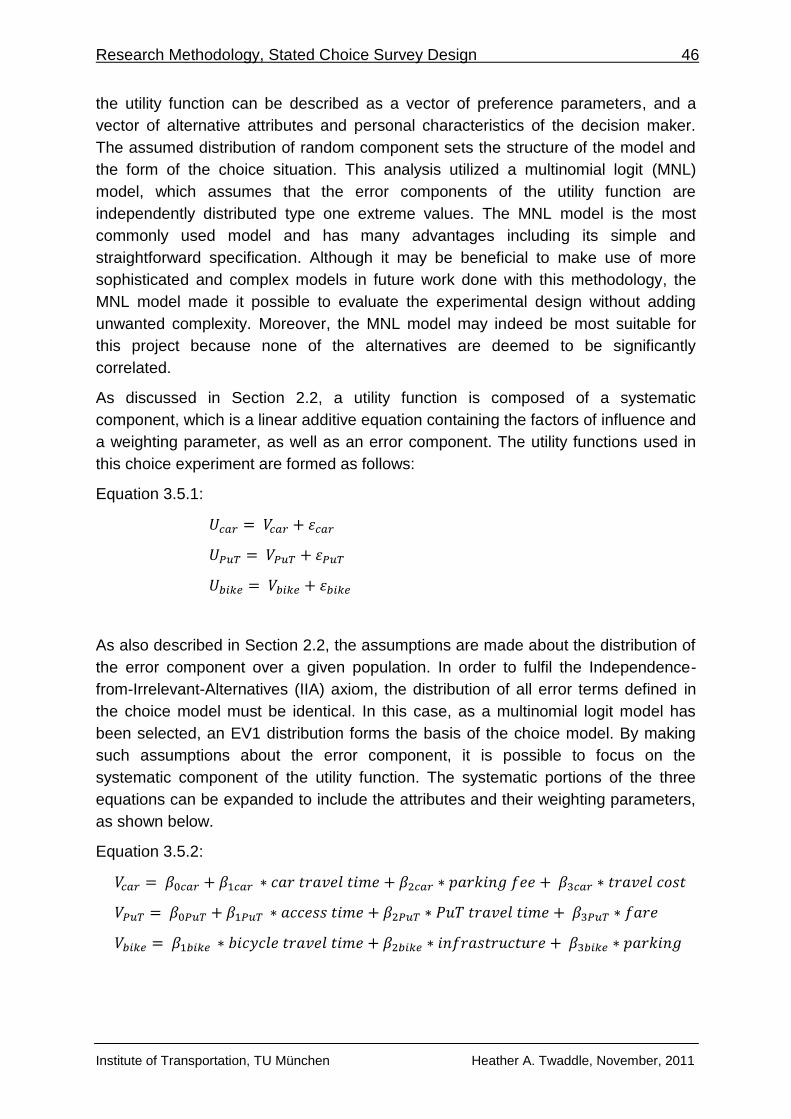
Research Methodology, Stated Choice Survey Design 46
Institute of Transportation, TU München Heather A. Twaddle, November, 2011
the utility function can be described as a vector of preference parameters, and a
vector of alternative attributes and personal characteristics of the decision maker.
The assumed distribution of random component sets the structure of the model and
the form of the choice situation. This analysis utilized a multinomial logit (MNL)
model, which assumes that the error components of the utility function are
independently distributed type one extreme values. The MNL model is the most
commonly used model and has many advantages including its simple and
straightforward specification. Although it may be beneficial to make use of more
sophisticated and complex models in future work done with this methodology, the
MNL model made it possible to evaluate the experimental design without adding
unwanted complexity. Moreover, the MNL model may indeed be most suitable for
this project because none of the alternatives are deemed to be significantly
correlated.
As discussed in Section 2.2, a utility function is composed of a systematic
component, which is a linear additive equation containing the factors of influence and
a weighting parameter, as well as an error component. The utility functions used in
this choice experiment are formed as follows:
Equation 3.5.1:
As also described in Section 2.2, the assumptions are made about the distribution of
the error component over a given population. In order to fulfil the Independence-
from-Irrelevant-Alternatives (IIA) axiom, the distribution of all error terms defined in
the choice model must be identical. In this case, as a multinomial logit model has
been selected, an EV1 distribution forms the basis of the choice model. By making
such assumptions about the error component, it is possible to focus on the
systematic component of the utility function. The systematic portions of the three
equations can be expanded to include the attributes and their weighting parameters,
as shown below.
Equation 3.5.2:
Research Methodology, Stated Choice Survey Design 47
Institute of Transportation, TU München Heather A. Twaddle, November, 2011
3.5.1. Using Revealed Data to Create the Stated Choice Experiment
An individualized stated choice situation was generated for each of the respondents
by selecting one of the reported trips in the time-use-travel diary. The trip was
selected based on the mode of transport used and the length of the trip. Research in
Germany has estimated that the mean maximum radius for non-motorized transport,
which is usually defined by bicycle use, is 4.6 km (Kuhnimhof, Chlond & Huang
2010). While the average person will select a motorized mode of transport for trips
reaching outside this radius, active modes of transportation are a viable option within
this radius. For this reason, reported trips that were less than 4.6 km were selected
with first priority for analysis. However, if a respondent did not report a trip less than
4.6 km in their time-use-travel diary, trips of all lengths were included as second
priority. The length of the trip was estimated using the origin and destination
addresses given by the respondent and the Google Maps © direction tool. The
second criterion for trip selection was the mode of transportation used by the
respondent. Because of the disproportionate number of bicycle trips reported in the
time-use-travel diaries, trips made by car were selected with first priority, followed by
those made by any mode of public transportation, and finally by those made by
bicycle. If a respondent did not make a trip using a car, bicycle or public transport,
they were excluded from the stated choice experiment.
The reference values used in the pivoted experimental design were taken from the
time-use-travel diaries. The coding of the time-use-travel diaries and the method
used to estimate the attribute levels of the alternatives that were not used in the
reported trip has been explained in Section 3.4. These values were used in
conjunction with the pivoted percentage values given in Table 2 to create the choice
situations for the respondents. A more detailed description of the data is found in
Table 3.
3.5.1. Segmentation of Respondents
In order to increase the rationality of stated choice survey and to limit the choice
situations to those that would yield useful statistical information, it was decided to
place some restriction on the assignment of the attribute levels based on the mode
the respondent reported using in the time-use-travel diary. This segmentation of
respondents was implemented for two reasons. Firstly, if the respondent was
presented with a choice situation that contained the alternative that they had used in
their reported trip, only with an increased overall utility, it was assumed that this
respondent would very likely choose this alternative again. This assumption is
aligned with the notion of utility balance, which dictates that a choice situation in a
stated choice experiment should contain alternatives with relatively comparable
overall utilities. If the respondent revealed a preference for one of the alternatives,
the theory of rational behaviour stipulates that this alternative held the most utility for
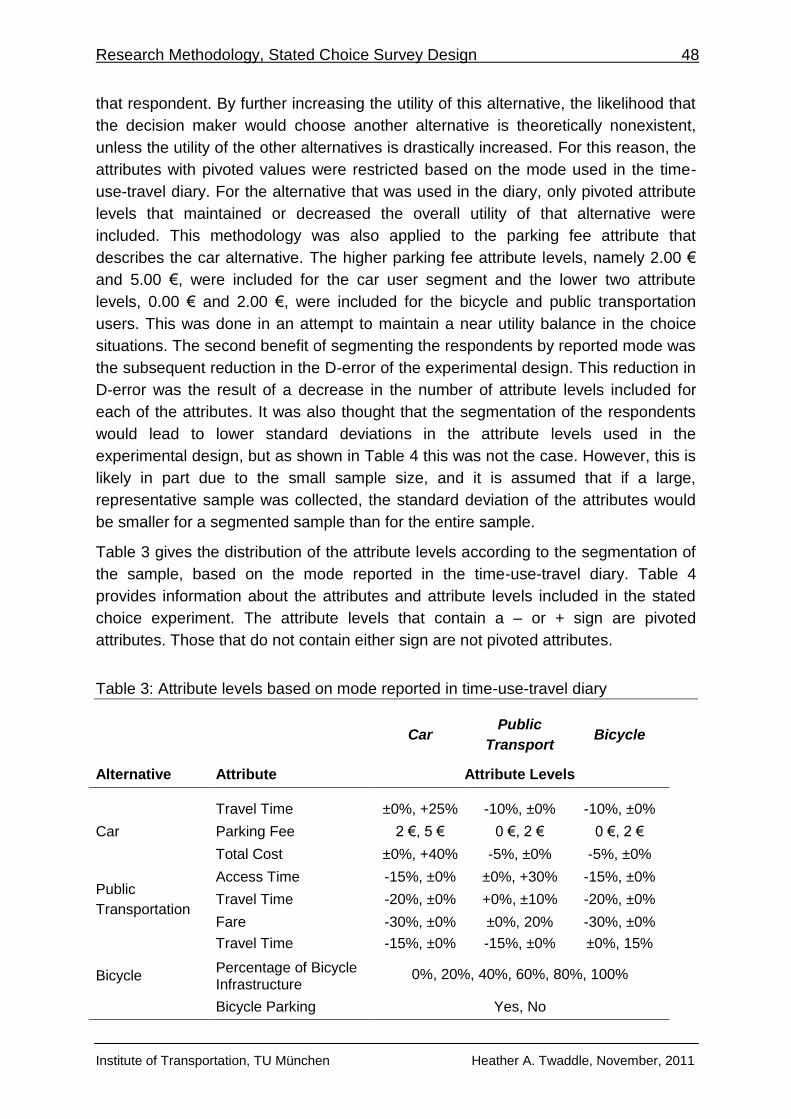
Research Methodology, Stated Choice Survey Design 48
Institute of Transportation, TU München Heather A. Twaddle, November, 2011
that respondent. By further increasing the utility of this alternative, the likelihood that
the decision maker would choose another alternative is theoretically nonexistent,
unless the utility of the other alternatives is drastically increased. For this reason, the
attributes with pivoted values were restricted based on the mode used in the time-
use-travel diary. For the alternative that was used in the diary, only pivoted attribute
levels that maintained or decreased the overall utility of that alternative were
included. This methodology was also applied to the parking fee attribute that
describes the car alternative. The higher parking fee attribute levels, namely 2.00 €
and 5.00 €, were included for the car user segment and the lower two attribute
levels, 0.00 € and 2.00 €, were included for the bicycle and public transportation
users. This was done in an attempt to maintain a near utility balance in the choice
situations. The second benefit of segmenting the respondents by reported mode was
the subsequent reduction in the D-error of the experimental design. This reduction in
D-error was the result of a decrease in the number of attribute levels included for
each of the attributes. It was also thought that the segmentation of the respondents
would lead to lower standard deviations in the attribute levels used in the
experimental design, but as shown in Table 4 this was not the case. However, this is
likely in part due to the small sample size, and it is assumed that if a large,
representative sample was collected, the standard deviation of the attributes would
be smaller for a segmented sample than for the entire sample.
Table 3 gives the distribution of the attribute levels according to the segmentation of
the sample, based on the mode reported in the time-use-travel diary. Table 4
provides information about the attributes and attribute levels included in the stated
choice experiment. The attribute levels that contain a – or + sign are pivoted
attributes. Those that do not contain either sign are not pivoted attributes.
Table 3: Attribute levels based on mode reported in time-use-travel diary
Car
Public
Transport Bicycle
Alternative Attribute Attribute Levels
Car
Travel Time ±0%, +25% -10%, ±0% -10%, ±0%
Parking Fee 2 €, 5 € 0 €, 2 € 0 €, 2 €
Total Cost ±0%, +40% -5%, ±0% -5%, ±0%
Public
Transportation
Access Time -15%, ±0% ±0%, +30% -15%, ±0%
Travel Time -20%, ±0% +0%, ±10% -20%, ±0%
Fare -30%, ±0% ±0%, 20% -30%, ±0%
Bicycle
Travel Time -15%, ±0% -15%, ±0% ±0%, 15%
Percentage of Bicycle Infrastructure
0%, 20%, 40%, 60%, 80%, 100%
Bicycle Parking Yes, No
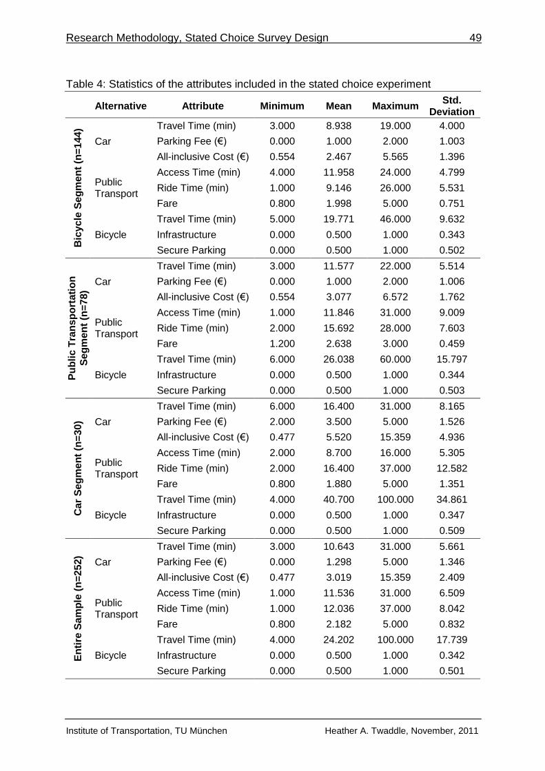
Research Methodology, Stated Choice Survey Design 49
Institute of Transportation, TU München Heather A. Twaddle, November, 2011
Table 4: Statistics of the attributes included in the stated choice experiment
Alternative Attribute Minimum Mean Maximum Std.
Deviation
Bic
yc
le S
eg
me
nt
(n=
144
)
Car
Travel Time (min) 3.000 8.938 19.000 4.000
Parking Fee (€) 0.000 1.000 2.000 1.003
All-inclusive Cost (€) 0.554 2.467 5.565 1.396
Public Transport
Access Time (min) 4.000 11.958 24.000 4.799
Ride Time (min) 1.000 9.146 26.000 5.531
Fare 0.800 1.998 5.000 0.751
Bicycle
Travel Time (min) 5.000 19.771 46.000 9.632
Infrastructure 0.000 0.500 1.000 0.343
Secure Parking 0.000 0.500 1.000 0.502
Pu
bli
c T
ran
sp
ort
ati
on
Se
gm
en
t (n
=7
8)
Car
Travel Time (min) 3.000 11.577 22.000 5.514
Parking Fee (€) 0.000 1.000 2.000 1.006
All-inclusive Cost (€) 0.554 3.077 6.572 1.762
Public Transport
Access Time (min) 1.000 11.846 31.000 9.009
Ride Time (min) 2.000 15.692 28.000 7.603
Fare 1.200 2.638 3.000 0.459
Bicycle
Travel Time (min) 6.000 26.038 60.000 15.797
Infrastructure 0.000 0.500 1.000 0.344
Secure Parking 0.000 0.500 1.000 0.503
Ca
r S
eg
me
nt
(n=
30
) Car
Travel Time (min) 6.000 16.400 31.000 8.165
Parking Fee (€) 2.000 3.500 5.000 1.526
All-inclusive Cost (€) 0.477 5.520 15.359 4.936
Public Transport
Access Time (min) 2.000 8.700 16.000 5.305
Ride Time (min) 2.000 16.400 37.000 12.582
Fare 0.800 1.880 5.000 1.351
Bicycle
Travel Time (min) 4.000 40.700 100.000 34.861
Infrastructure 0.000 0.500 1.000 0.347
Secure Parking 0.000 0.500 1.000 0.509
En
tire
Sa
mp
le (
n=
25
2)
Car
Travel Time (min) 3.000 10.643 31.000 5.661
Parking Fee (€) 0.000 1.298 5.000 1.346
All-inclusive Cost (€) 0.477 3.019 15.359 2.409
Public Transport
Access Time (min) 1.000 11.536 31.000 6.509
Ride Time (min) 1.000 12.036 37.000 8.042
Fare 0.800 2.182 5.000 0.832
Bicycle
Travel Time (min) 4.000 24.202 100.000 17.739
Infrastructure 0.000 0.500 1.000 0.342
Secure Parking 0.000 0.500 1.000 0.501
Research Methodology, Stated Choice Survey Design 50
Institute of Transportation, TU München Heather A. Twaddle, November, 2011
3.5.2. Experimental Design
Once the alternatives, attributes and attribute levels were defined and the model
specification was decided upon, it was possible to continue with the experimental
design of the choice experiment. Before the design was begun, the theory of stated
choice experimental design was thoroughly reviewed and a comprehensive overview
is presented in Section 2.3. After reviewing the classes of design that are available
for stated choice experiments, an efficient design was selected because of the
statistical advantages characteristic of this design class. It is arguable that when
estimates of the β parameters of the utility functions are available, an efficient design
will always be statistically superior to an orthogonal fractional factorial design, even if
these estimates are only the sign of the parameter (ChoiceMetrics 2011). Because
all of the β parameters included in the utility functions specified for this model
(Equation 3.5.2) could either be roughly estimated from the results of previous
experiments, or could be derived from these results, an efficient design was
selected. Efficient designs are particularly well suited for experiments that
incorporate pivoting attribute levels. The advantage of using efficient designs over
orthogonal fractional factorial designs in experiments with pivoted attribute levels is
the propensity for utility balance among the alternatives in a choice situation. This
tendency toward utility balance is important because of the large range of attribute
values taken from the revealed preference data. Indeed, efficient designs are the
only type of experimental design that are recommended for pivoted attribute
experiments by the authors of the Ngene user manual (ChoiceMetrics 2011, pp. 157-
169). In a comparison of design methods that were applied to stated choice
experiments built from revealed preference data, Rose et al. (2008, p. 402) noted
that “overall, the orthogonal design performed very poorly when applied to the
empirical data set”.
In order to use an efficient design for this experiment, it was necessary to identify β
parameters in previous studies that could be used as base estimates. An attempt
was made to locate studies undertaken in or near Germany to account for
differences in transportation behaviour between different countries. However, it was
not possible to locate European literature that quantitatively investigated the β
parameters for all of the attributes. In these cases, β parameters from other counties
(namely Chile and Canada) were used. The use of these parameters is justified by
the fact that only rough estimates are required for the efficient design (particularly if a
Bayesian method is employed).Although the β constants used in the car and public
transportation alternative utility functions have been included for completeness, the
Ngene user manual states that due to the large standard deviations characteristic of
constants, such values should not be included in the D-error calculation
(ChoiceMetrics 2011, p. 92). Estimates of the β parameter for each attribute, the
literature source they were adopted from and any notes concerning the use of the β
parameters have been included in Tables 5, 6 and 7.
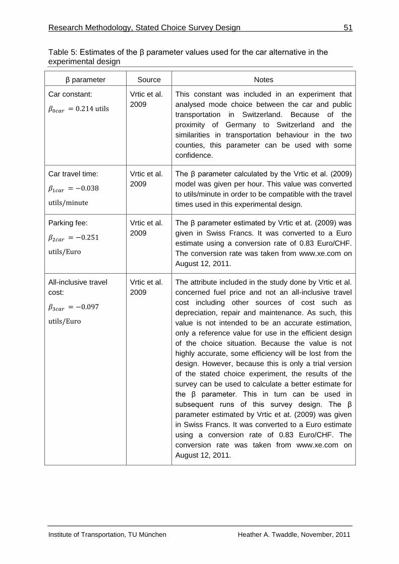
Research Methodology, Stated Choice Survey Design 51
Institute of Transportation, TU München Heather A. Twaddle, November, 2011
Table 5: Estimates of the β parameter values used for the car alternative in the experimental design
β parameter Source Notes
Car constant:
Vrtic et al.
2009
This constant was included in an experiment that
analysed mode choice between the car and public
transportation in Switzerland. Because of the
proximity of Germany to Switzerland and the
similarities in transportation behaviour in the two
counties, this parameter can be used with some
confidence.
Car travel time:
Vrtic et al.
2009
The β parameter calculated by the Vrtic et al. (2009)
model was given per hour. This value was converted
to utils/minute in order to be compatible with the travel
times used in this experimental design.
Parking fee:
Vrtic et al.
2009
The β parameter estimated by Vrtic et at. (2009) was
given in Swiss Francs. It was converted to a Euro
estimate using a conversion rate of 0.83 Euro/CHF.
The conversion rate was taken from www.xe.com on
August 12, 2011.
All-inclusive travel
cost:
Vrtic et al.
2009
The attribute included in the study done by Vrtic et al.
concerned fuel price and not an all-inclusive travel
cost including other sources of cost such as
depreciation, repair and maintenance. As such, this
value is not intended to be an accurate estimation,
only a reference value for use in the efficient design
of the choice situation. Because the value is not
highly accurate, some efficiency will be lost from the
design. However, because this is only a trial version
of the stated choice experiment, the results of the
survey can be used to calculate a better estimate for
the β parameter. This in turn can be used in
subsequent runs of this survey design. The β
parameter estimated by Vrtic et at. (2009) was given
in Swiss Francs. It was converted to a Euro estimate
using a conversion rate of 0.83 Euro/CHF. The
conversion rate was taken from www.xe.com on
August 12, 2011.
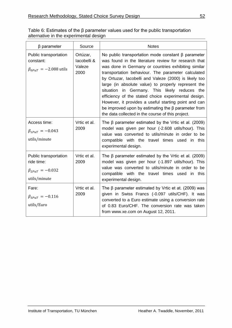
Research Methodology, Stated Choice Survey Design 52
Institute of Transportation, TU München Heather A. Twaddle, November, 2011
Table 6: Estimates of the β parameter values used for the public transportation alternative in the experimental design
β parameter Source Notes
Public transportation
constant:
Ortúzar,
Iacobelli &
Valeze
2000
No public transportation mode constant β parameter
was found in the literature review for research that
was done in Germany or countries exhibiting similar
transportation behaviour. The parameter calculated
by Ortuzar, Iacobelli and Valeze (2000) is likely too
large (in absolute value) to properly represent the
situation in Germany. This likely reduces the
efficiency of the stated choice experimental design.
However, it provides a useful starting point and can
be improved upon by estimating the β parameter from
the data collected in the course of this project.
Access time:
Vrtic et al.
2009
The β parameter estimated by the Vrtic et al. (2009)
model was given per hour (-2.608 utils/hour). This
value was converted to utils/minute in order to be
compatible with the travel times used in this
experimental design.
Public transportation
ride time:
Vrtic et al.
2009
The β parameter estimated by the Vrtic et al. (2009)
model was given per hour (-1.897 utils/hour). This
value was converted to utils/minute in order to be
compatible with the travel times used in this
experimental design.
Fare:
Vrtic et al.
2009
The β parameter estimated by Vrtic et at. (2009) was
given in Swiss Francs (-0.097 utils/CHF). It was
converted to a Euro estimate using a conversion rate
of 0.83 Euro/CHF. The conversion rate was taken
from www.xe.com on August 12, 2011.
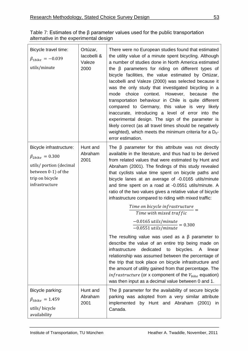
Research Methodology, Stated Choice Survey Design 53
Institute of Transportation, TU München Heather A. Twaddle, November, 2011
Table 7: Estimates of the β parameter values used for the public transportation alternative in the experimental design
Bicycle travel time:
Ortúzar,
Iacobelli &
Valeze
2000
There were no European studies found that estimated
the utility value of a minute spent bicycling. Although
a number of studies done in North America estimated
the β parameters for riding on different types of
bicycle facilities, the value estimated by Ortúzar,
Iacobelli and Valeze (2000) was selected because it
was the only study that investigated bicycling in a
mode choice context. However, because the
transportation behaviour in Chile is quite different
compared to Germany, this value is very likely
inaccurate, introducing a level of error into the
experimental design. The sign of the parameter is
likely correct (as all travel times should be negatively
weighted), which meets the minimum criteria for a Db-
error estimation.
Bicycle infrastructure:
utils/ portion (decimal
between 0-1) of the
trip on bicycle
infrastructure
Hunt and
Abraham
2001
The β parameter for this attribute was not directly
available in the literature, and thus had to be derived
from related values that were estimated by Hunt and
Abraham (2001). The findings of this study revealed
that cyclists value time spent on bicycle paths and
bicycle lanes at an average of -0.0165 utils/minute
and time spent on a road at -0.0551 utils/minute. A
ratio of the two values gives a relative value of bicycle
infrastructure compared to riding with mixed traffic:
The resulting value was used as a β parameter to
describe the value of an entire trip being made on
infrastructure dedicated to bicycles. A linear
relationship was assumed between the percentage of
the trip that took place on bicycle infrastructure and
the amount of utility gained from that percentage. The
(or x component of the equation)
was then input as a decimal value between 0 and 1.
Bicycle parking:
utils/ bicycle
availability
Hunt and
Abraham
2001
The β parameter for the availability of secure bicycle
parking was adopted from a very similar attribute
implemented by Hunt and Abraham (2001) in
Canada.
Research Methodology, Stated Choice Survey Design 54
Institute of Transportation, TU München Heather A. Twaddle, November, 2011
Although the advantages of using efficient designs for experiments with pivoted
attribute levels are well known, the incorporation of pivoted attribute levels based on
revealed preference data are unfortunately not completely supported by the current
methods of generating choice experiments (Rose et al. 2008). For this reason, the
experimental design was created using a combination of Excel and Ngene. Once the
attributes, attribute levels and segmentation were decided upon, it was possible to
create an Excel file that combined the reference value data and the pivot level
information to create the choice situations. Firstly, a matrix was set up containing the
reference scenario for all the respondents. These values were either taken directly
from the time-use-travel diary or were estimated using the origin and destination
location (using the method described in Table 1). The attribute levels for the non-
pivoting attributes (parking fee, dedicated bicycle infrastructure and bicycle parking)
and the pivot percentages for the pivoting attributes (all other attributes) were input
into a second matrix. The matrices were then combined to create a single matrix
containing the attribute level values for all the respondents. These values were then
taken in combination with the estimated β parameters to create the code input into
Ngene to develop an efficient experimental design. The code was created following
the methodology suggested in the Ngene user manual (ChoiceMetrics 2011, pp. 157-
169). The Excel file that was used to create the Ngene code is included on the CD
that accompanies this thesis report (file: Ngene code builder.xlsx).
In order to create individualized choice situations for all of the respondents, it was
necessary to utilize a method for building choice sets with different reference values
and hence different attribute levels into the same experimental design. This can be
done using Ngene in two ways. According to ChoiceMetrics (2011), the first method,
known as a homogeneous pivot design, generates a single design that can be used
for all respondents while applying their different attribute level values. The second
method, heterogeneous pivot design, generates a new experimental design for each
of the respondents based on the notion that different segments face different
reference alternatives (ChoiceMetrics 2011). For both types of pivot design, a fisher
information matrix (or the determinant of the AVC matrix) must be specified along
with the weight given to each data segment. A combination of both types of pivot
design is also possible and was implemented in this experimental design. The
respondents were grouped into three segments; those who used the car for their
reported trip, those who used a bicycle and those who used public transportation. A
heterogeneous pivot design was built to account for the fact that these segments
selected different reference modes. In addition, the different segments were faced
with different attribute levels, as shown in Table 3, and as such could not be included
in a homogeneous design. However, within each of the segments, a homogeneous
pivot design was used because the respondents did not face different reference
alternatives. Each of the respondents was given the same weighting in the fisher
information matrix. The resulting form of the fisher matrix is shown in Equation 3.5.3.
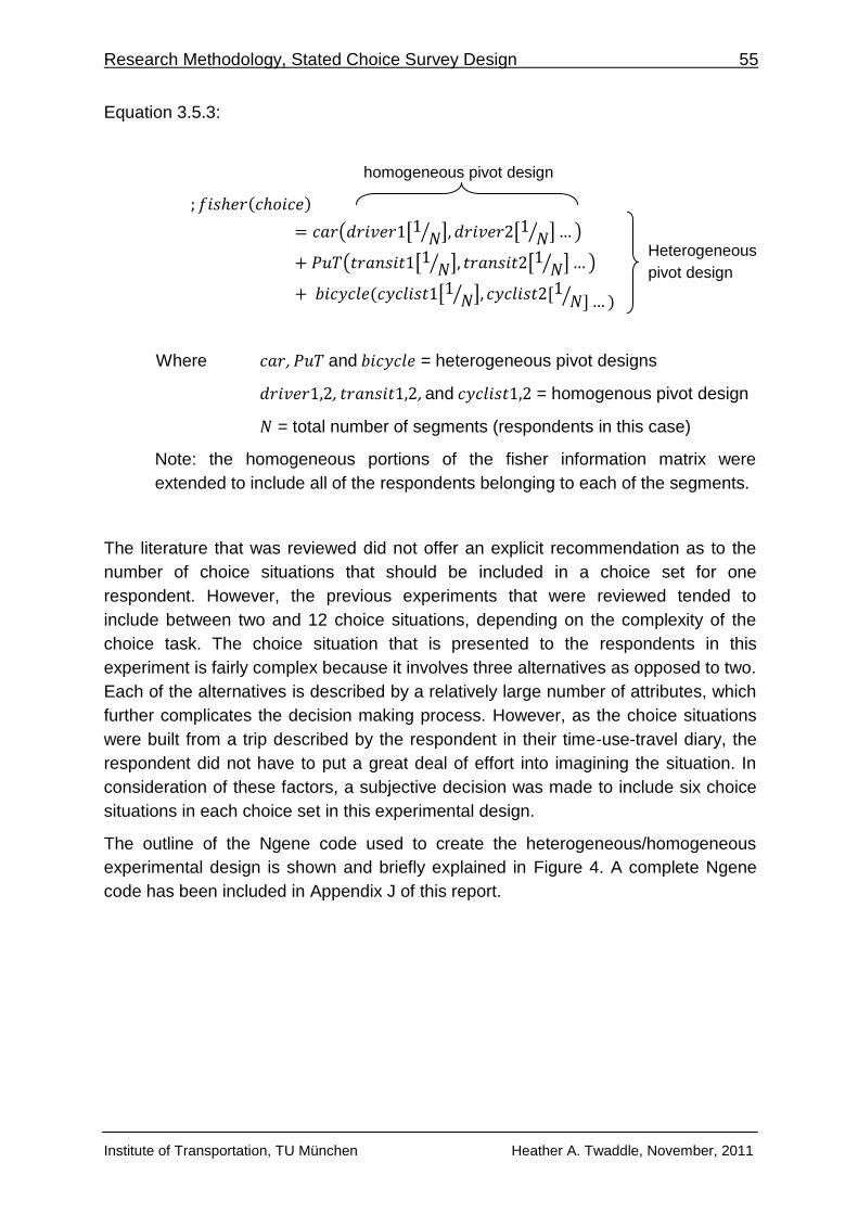
Research Methodology, Stated Choice Survey Design 55
Institute of Transportation, TU München Heather A. Twaddle, November, 2011
Equation 3.5.3:
homogeneous pivot design
Heterogeneous
pivot design
Where , and = heterogeneous pivot designs
, , and = homogenous pivot design
= total number of segments (respondents in this case)
Note: the homogeneous portions of the fisher information matrix were
extended to include all of the respondents belonging to each of the segments.
The literature that was reviewed did not offer an explicit recommendation as to the
number of choice situations that should be included in a choice set for one
respondent. However, the previous experiments that were reviewed tended to
include between two and 12 choice situations, depending on the complexity of the
choice task. The choice situation that is presented to the respondents in this
experiment is fairly complex because it involves three alternatives as opposed to two.
Each of the alternatives is described by a relatively large number of attributes, which
further complicates the decision making process. However, as the choice situations
were built from a trip described by the respondent in their time-use-travel diary, the
respondent did not have to put a great deal of effort into imagining the situation. In
consideration of these factors, a subjective decision was made to include six choice
situations in each choice set in this experimental design.
The outline of the Ngene code used to create the heterogeneous/homogeneous
experimental design is shown and briefly explained in Figure 4. A complete Ngene
code has been included in Appendix J of this report.
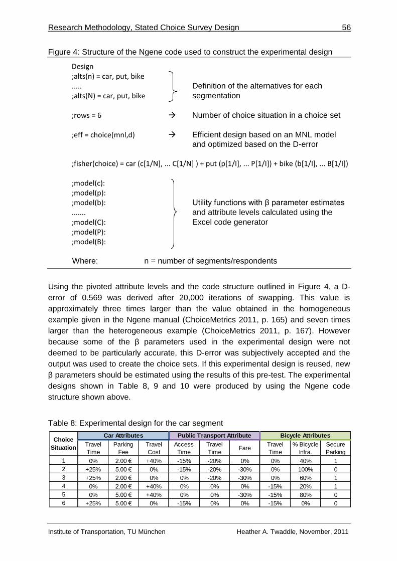
Research Methodology, Stated Choice Survey Design 56
Institute of Transportation, TU München Heather A. Twaddle, November, 2011
Figure 4: Structure of the Ngene code used to construct the experimental design
Design ;alts(n) = car, put, bike ..... Definition of the alternatives for each
;alts(N) = car, put, bike segmentation ;rows = 6 Number of choice situation in a choice set
;eff = choice(mnl,d) Efficient design based on an MNL model
and optimized based on the D-error
;fisher(choice) = car (c[1/N], ... C[1/N] ) + put (p[1/I], ... P[1/I]) + bike (b[1/I], ... B[1/I]) ;model(c): ;model(p): ;model(b): Utility functions with β parameter estimates ....... and attribute levels calculated using the ;model(C): Excel code generator ;model(P): ;model(B):
Where: n = number of segments/respondents
Using the pivoted attribute levels and the code structure outlined in Figure 4, a D-
error of 0.569 was derived after 20,000 iterations of swapping. This value is
approximately three times larger than the value obtained in the homogeneous
example given in the Ngene manual (ChoiceMetrics 2011, p. 165) and seven times
larger than the heterogeneous example (ChoiceMetrics 2011, p. 167). However
because some of the β parameters used in the experimental design were not
deemed to be particularly accurate, this D-error was subjectively accepted and the
output was used to create the choice sets. If this experimental design is reused, new
β parameters should be estimated using the results of this pre-test. The experimental
designs shown in Table 8, 9 and 10 were produced by using the Ngene code
structure shown above.
Table 8: Experimental design for the car segment
Travel
Time
Parking
Fee
Travel
Cost
Access
Time
Travel
TimeFare
Travel
Time
% Bicycle
Infra.
Secure
Parking
1 0% 2.00 € +40% -15% -20% 0% 0% 40% 1
2 +25% 5.00 € 0% -15% -20% -30% 0% 100% 0
3 +25% 2.00 € 0% 0% -20% -30% 0% 60% 1
4 0% 2.00 € +40% 0% 0% 0% -15% 20% 1
5 0% 5.00 € +40% 0% 0% -30% -15% 80% 0
6 +25% 5.00 € 0% -15% 0% 0% -15% 0% 0
Choice
Situation
Car Attributes Public Transport Attribute Bicycle Attributes
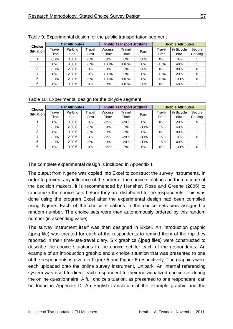
Research Methodology, Stated Choice Survey Design 57
Institute of Transportation, TU München Heather A. Twaddle, November, 2011
Table 9: Experimental design for the public transportation segment
Table 10: Experimental design for the bicycle segment
The complete experimental design is included in Appendix I.
The output from Ngene was copied into Excel to construct the survey instruments. In
order to prevent any influence of the order of the choice situations on the outcome of
the decision makers, it is recommended by Hensher, Rose and Greene (2005) to
randomize the choice sets before they are distributed to the respondents. This was
done using the program Excel after the experimental design had been compiled
using Ngene. Each of the choice situations in the choice sets was assigned a
random number. The choice sets were then autonomously ordered by this random
number (in ascending value).
The survey instrument itself was then designed in Excel. An introduction graphic
(.jpeg file) was created for each of the respondents to remind them of the trip they
reported in their time-use-travel diary. Six graphics (.jpeg files) were constructed to
describe the choice situations in the choice set for each of the respondents. An
example of an introduction graphic and a choice situation that was presented to one
of the respondents is given in Figure 5 and Figure 6 respectively. The graphics were
each uploaded onto the online survey instrument, Unipark. An internal referencing
system was used to direct each respondent to their individualized choice set during
the online questionnaire. A full choice situation, as presented to one respondent, can
be found in Appendix D. An English translation of the example graphic and the
Travel
Time
Parking
Fee
Travel
Cost
Access
Time
Travel
TimeFare
Travel
Time
% Bicycle
Infra.
Secure
Parking
1 -10% 0.00 € -5% 0% 0% 20% 0% 0% 1
2 0% 0.00 € -5% +30% +10% 0% -15% 40% 1
3 -10% 2.00 € 0% 0% 0% 20% 0% 80% 0
4 0% 2.00 € 0% +30% 0% 0% -15% 20% 0
5 -10% 2.00 € -5% +30% +10% 0% -15% 100% 0
6 0% 0.00 € 0% 0% +10% 20% 0% 60% 1
Choice
Situation
Car Attributes Public Transport Attribute Bicycle Attributes
Travel
Time
Parking
Fee
Travel
Cost
Access
Time
Travel
TimeFare
Travel
Time
% Bicycle
Infra.
Secure
Parking
1 0% 0.00 € 0% -15% -20% 0% 0% 20% 0
2 -10% 2.00 € -5% 0% 0% -30% +15% 60% 1
3 0% 0.00 € -5% 0% 0% 0% 0% 80% 1
4 -10% 2.00 € 0% -15% -20% -30% +15% 0% 0
5 -10% 2.00 € -5% 0% -20% -30% +15% 40% 1
6 0% 0.00 € 0% -15% 0% 0% 0% 100% 0
Bicycle AttributesChoice
Situation
Car Attributes Public Transport Attribute
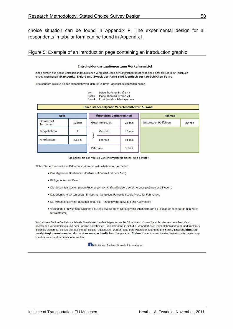
Research Methodology, Stated Choice Survey Design 58
Institute of Transportation, TU München Heather A. Twaddle, November, 2011
choice situation can be found in Appendix F. The experimental design for all
respondents in tabular form can be found in Appendix I.
Figure 5: Example of an introduction page containing an introduction graphic

Research Methodology, Stated Choice Survey Design 59
Institute of Transportation, TU München Heather A. Twaddle, November, 2011
Figure 6: Example of a choice situation as presented to a respondent
Research Methodology, Personal Survey 60
Institute of Transportation, TU München Heather A. Twaddle, November, 2011
3.6. Personal Survey
A personal survey was distributed in addition to the time-use-travel diary and the
stated choice experiment to collect socio-economic information from the
respondents. It was necessary to collect this information because according to the
theory of discrete choice, the utility of an alternative is defined by both the socio-
economic characteristics of the decision maker and the choice task factors (or the
alternatives and attributes of those alternatives) (Hensher & Greene 2003). It was not
possible to collect information on a household level for this project because the
survey was distributed to individual people rather than entire households. There were
only a couple of cases where all members of a household responded to the survey.
The questions in the personal questionnaire were adapted from personal and
household questionnaires that were written and distributed by the Mobilität in
Deutschland, which is a country-wide transportation research project carried out in
Germany (Mobilität in Deutschland 2010). Socio-economic information collected in
the personal questionnaire included age, gender, income, level of education, current
employment status, and the current living situation (alone, with a partner or children,
etc.). Information concerning personal transportation behaviour was also collected
including: the frequency of car, public transportation and bicycle use, the walking
time from the household to the nearest bus, tram and U-Bahn / S-Bahn / regional
train station, the type of public transportation ticket used most frequently, the
ownership of a bicycle, the number of cars in the household, the size of the car if
there was a car in the household, and availability of that car to the respondent, the
reason for not owning a car if there was no car in the household, and the possession
of a valid driver‟s licence. An additional question was included that enquired about
the importance of safety, comfort, convenience, flexibility and environmental impact
on the mode choice decision. The complete survey as distributed to the respondents
(in German) can be found in Appendix D. An English translation of the survey has
been included in Appendix E.
The personal questionnaire was distributed online with the stated choice experiment
rather than as a paper and pencil survey with the time-use-travel diary. This decision
was made in an attempt to reduce the workload of the respondents, save paper and
capitalize on automatic coding. The only drawback of this decision was that no
personal information was collected from respondents who filled out a time-use-travel
diary but failed to complete the second portion of the survey. The online personal
survey was developed using the online survey program Unipark (Globalpark AG
2011).
Research Methodology, Stated Choice and Personal Questionnaire Distribution 61
Institute of Transportation, TU München Heather A. Twaddle, November, 2011
3.7. Stated Choice and Personal Questionnaire Distribution
The personal questionnaire and the stated choice experiment were distributed to the
respondents as a single online survey. An online survey instrument, Unipark, was
used to construct and distribute the personal questionnaire and the stated choice
experiment. The personal questionnaire questions were created using the various
pre-programmed question formats that are offered by Unipark. The stated choice
information page and the choice situations were constructed using the user defined
question format. An html code was written to display a .jpeg file. As described in
Section 3.5, each of the choice situations were formatted in Excel and were saved
individually as .jpeg files. These .jpeg files were then uploaded into the Unipark
media folder according to the respondent ID. A total of 301 .jpeg files were created
and uploaded into the Unipark media folder. The html code written for stated choice
information and choice situations incorporated a dynamic element, known as a
wildcard in Unipark, to select the appropriate .jpeg file based on the respondent ID.
Using Unipark, it is possible to create and distribute surveys to a predetermined
sample of people. As the stated choice experiments were individualized for the
respondents, it was important to make use of this feature for this survey. The
respondents name and email, documented on the time-use-travel diary by the
respondent, was used to create individual respondent profiles in Unipark. A
respondent ID, or group number in Unipark, was assigned to each respondent so
that the choice sets could be organized. This information also made it possible to
email a link to the survey and a password for accessing the survey to the
respondents.
Using Unipark, a link to the online survey and a password was emailed automatically
to the 48 people who had returned a time-use-travel diary on September 23rd, 2011.
A link containing only the personal questionnaire was sent to the five respondents
who did not submit enough information or did not make any trips long enough to
construct a choice experiment. A reminder email was sent to the 12 participants who
had not yet completed the survey on October 10th, 2011.

Results, Response to the Survey 62
Institute of Transportation, TU München Heather A. Twaddle, November, 2011
4. RESULTS
The following section summarizes the results of the time-use-travel diary and the
stated choice experiment. A selection of descriptive analysis of the data collected is
also provided. However, as the objective of the thesis is to provide a qualitative
assessment of the survey instruments, an in depth descriptive or inferential statistical
analysis is not undertaken.
4.1. Response to the Survey
A total of 97 time-use-travel packages were distributed to potential survey
participants. However, of these 97 packages, only 56 were distributed to people who
had agreed to take part in the survey before receiving a survey package. The rest of
the packages were given to the family, friends and colleagues of the seven survey
respondents who had agreed to further distribute survey packages. A total of 48
time-use-travel diaries were completed and returned by mail, accounting for a 49%
return rate for the first phase of the survey process for all survey packages that were
prepared10. However, when considering that only 56 people agreed to participate
before they were given a survey package (44 people originally and 12 people in the
following weeks), the response rate increases to 86%.
Of the 48 people who returned a time-use-travel diary, 5 people failed to include
addresses for their activities. Individualized stated choice experiments were created
for the remaining 43 respondent. Of those 43 respondents, 40 completed the online
personal questionnaire and stated choice experiment, accounting for a second
phase response rate of 93% for the people who correctly filled out the time-use-
travel diary. Although a stated choice experiment could not be created for the people
who did not correctly fill out their time-use-travel diary, these five people were still
sent a personal questionnaire online. Of these five people, four completed the online
survey.
10 This figure excludes the response rate of the survey invitation letters that were sent to the 500
purchased addresses and the emails that were sent to friends and family of the research team.

Results, Time-Use-Travel Diary Results 63
Institute of Transportation, TU München Heather A. Twaddle, November, 2011
4.2. Time-Use-Travel Diary Results
The time-use-travel diaries were analysed to provide an overview of the trips
recorded by the respondents. Of the 48 people who returned time-use-travel diaries,
45 diaries could be coded. The three diaries that could not be coded did not contain
any origin and destination information. Two diaries contained all the necessary
information for coding but consisted only of walking trips. As mentioned in Section
3.5, walking trips were not included in the stated choice experiment because the
length of these trips is usually too short to compete with the car or public
transportation. They were, however, included in the analysis of the time-use-travel
diaries. A total of 227 trips were reported in the 45 valid time-use-travel diaries.
However, trips were omitted from analysis if the respondent did not spend at least
one minute at a destination. These trips were omitted because they were made for
another reason other than utilitarian travel and would likely not be substituted with
another mode of transportation. A total of 224 utilitarian trips remained in the dataset.
Table 11 provides a statistical summary of the data collected in the time-use-travel
diaries.
The mode of transportation reported by the respondent is important to consider
because the respondents were segmented based on this factor. More than half of
the trips reported by respondents in their time use travel diaries were made using a
bicycle. The mode of transportation used for the reported trips is shown in Figure 7.
The actual modal splits of the four modes estimated in 2010 by the City of Munich
(Landeshauptstadt München 2010) are bracketed after the mode label. The
proportion of reported trips made by bicycle in this survey is considerably higher than
the 14% of trips that are made by bicycle in Munich according to the City of Munich
(Landeshauptstadt München 2010). This is likely due to the fact that the survey was
advertised as focusing on bicycling in Munich, and as such, respondents who are
particularity interested and active in bicycling were likely more inclined to participate
in the survey.
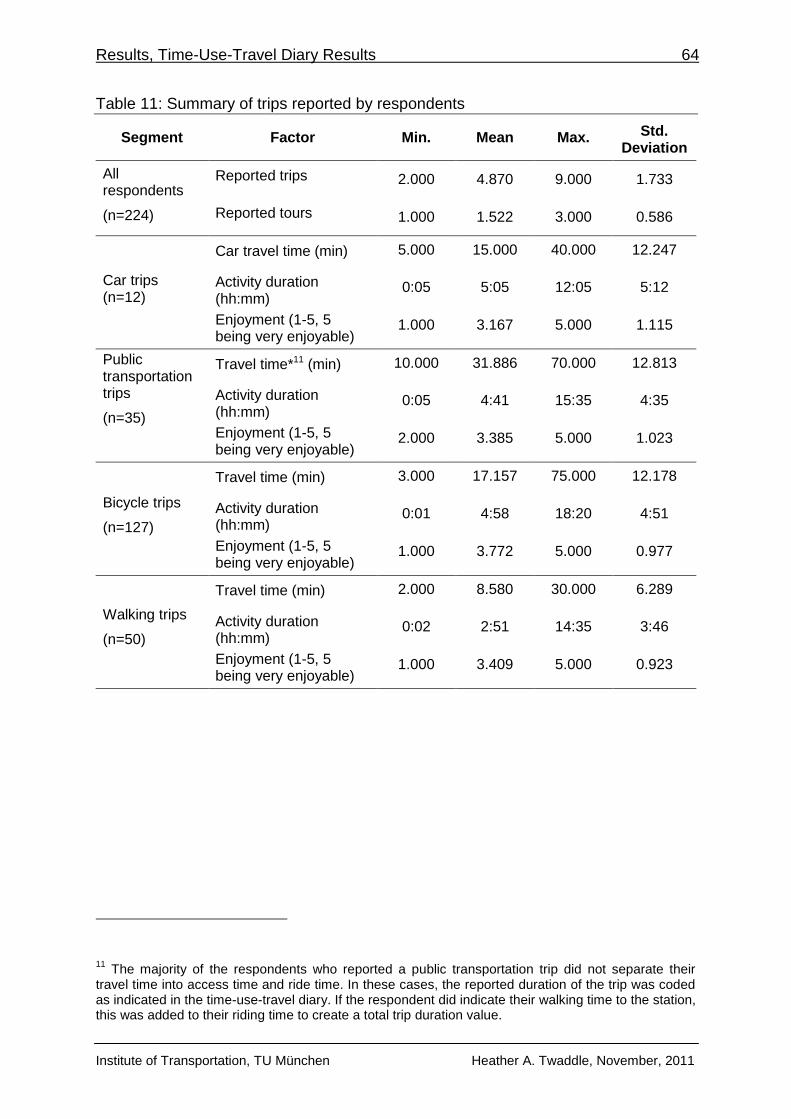
Results, Time-Use-Travel Diary Results 64
Institute of Transportation, TU München Heather A. Twaddle, November, 2011
Table 11: Summary of trips reported by respondents
Segment Factor Min. Mean Max. Std. Deviation
All respondents
(n=224)
Reported trips 2.000 4.870 9.000 1.733
Reported tours 1.000 1.522 3.000 0.586
Car trips (n=12)
Car travel time (min) 5.000 15.000 40.000 12.247
Activity duration (hh:mm)
0:05 5:05 12:05 5:12
Enjoyment (1-5, 5 being very enjoyable)
1.000 3.167 5.000 1.115
Public transportation trips
(n=35)
Travel time*11 (min) 10.000 31.886 70.000 12.813
Activity duration (hh:mm)
0:05 4:41 15:35 4:35
Enjoyment (1-5, 5 being very enjoyable)
2.000 3.385 5.000 1.023
Bicycle trips
(n=127)
Travel time (min) 3.000 17.157 75.000 12.178
Activity duration (hh:mm)
0:01 4:58 18:20 4:51
Enjoyment (1-5, 5 being very enjoyable)
1.000 3.772 5.000 0.977
Walking trips
(n=50)
Travel time (min) 2.000 8.580 30.000 6.289
Activity duration (hh:mm)
0:02 2:51 14:35 3:46
Enjoyment (1-5, 5 being very enjoyable)
1.000 3.409 5.000 0.923
11 The majority of the respondents who reported a public transportation trip did not separate their
travel time into access time and ride time. In these cases, the reported duration of the trip was coded as indicated in the time-use-travel diary. If the respondent did indicate their walking time to the station, this was added to their riding time to create a total trip duration value.
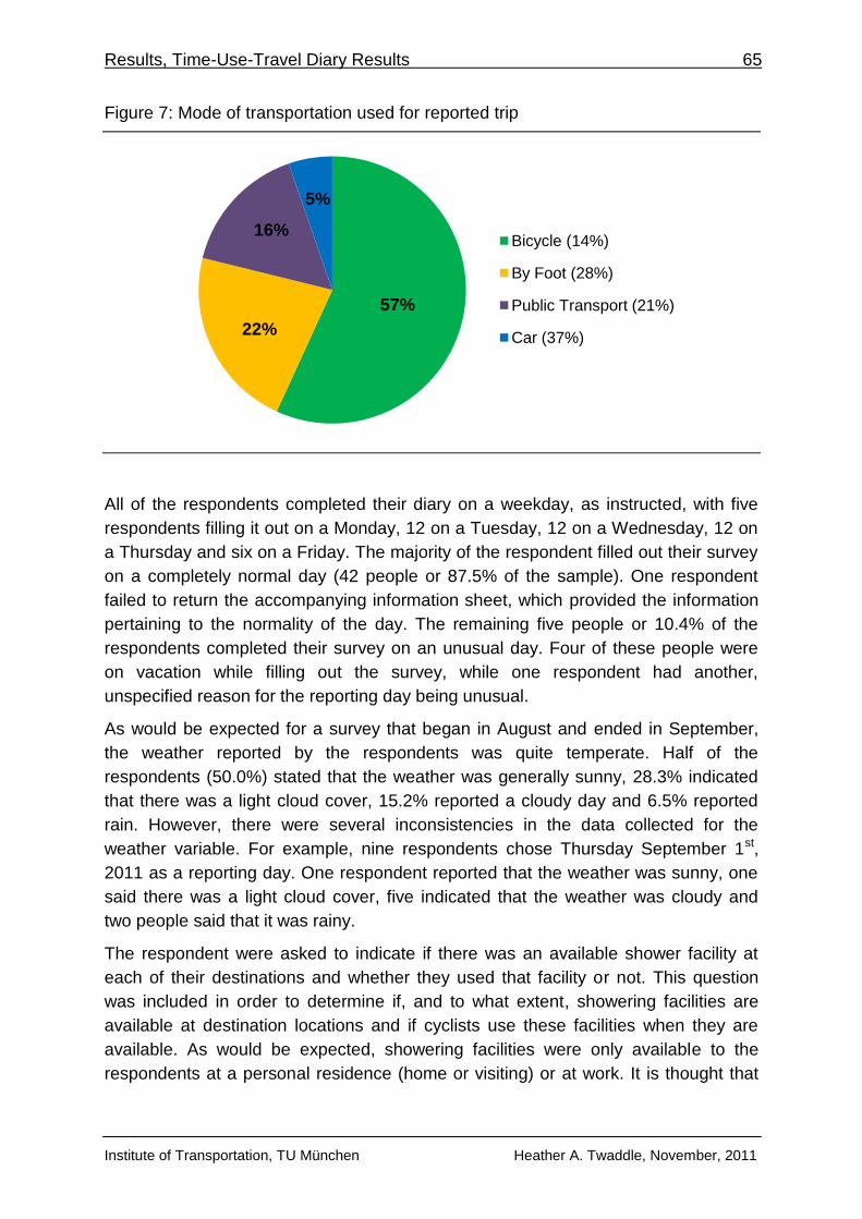
Results, Time-Use-Travel Diary Results 65
Institute of Transportation, TU München Heather A. Twaddle, November, 2011
Figure 7: Mode of transportation used for reported trip
All of the respondents completed their diary on a weekday, as instructed, with five
respondents filling it out on a Monday, 12 on a Tuesday, 12 on a Wednesday, 12 on
a Thursday and six on a Friday. The majority of the respondent filled out their survey
on a completely normal day (42 people or 87.5% of the sample). One respondent
failed to return the accompanying information sheet, which provided the information
pertaining to the normality of the day. The remaining five people or 10.4% of the
respondents completed their survey on an unusual day. Four of these people were
on vacation while filling out the survey, while one respondent had another,
unspecified reason for the reporting day being unusual.
As would be expected for a survey that began in August and ended in September,
the weather reported by the respondents was quite temperate. Half of the
respondents (50.0%) stated that the weather was generally sunny, 28.3% indicated
that there was a light cloud cover, 15.2% reported a cloudy day and 6.5% reported
rain. However, there were several inconsistencies in the data collected for the
weather variable. For example, nine respondents chose Thursday September 1st,
2011 as a reporting day. One respondent reported that the weather was sunny, one
said there was a light cloud cover, five indicated that the weather was cloudy and
two people said that it was rainy.
The respondent were asked to indicate if there was an available shower facility at
each of their destinations and whether they used that facility or not. This question
was included in order to determine if, and to what extent, showering facilities are
available at destination locations and if cyclists use these facilities when they are
available. As would be expected, showering facilities were only available to the
respondents at a personal residence (home or visiting) or at work. It is thought that
57%
22%
16%
5%
Bicycle (14%)
By Foot (28%)
Public Transport (21%)
Car (37%)

Results, Time-Use-Travel Diary Results 66
Institute of Transportation, TU München Heather A. Twaddle, November, 2011
the 7% of respondents who indicated that no shower was available upon their return
home misunderstood the question or made a mistake in filling out the diary.
4.3. Stated Choice Experiment Results
A total of 40 respondents completed the stated choice experiment, and as each
choice experiment included six choice situations, choice data was collected for 240
choice situations. Of the 240 decisions that were made, 151 (62.9%) were made for
the bicycle, 62 (25.8%) were made for public transport, and 27 (11.3%) were made
for the car. When facing the choice situations 167 respondents (69.6%) selected the
same mode as they used for their reported trip. If the respondent selected the same
mode for all of the choice situations that they faced, and this selected mode was the
same as the mode used in their reported trip, the respondent was asked if it would
be possible for them to switch modes in any situation. Of the 40 respondents, 17
(38.6%) decided for the same mode as they used in their reported trip for all six of
the choice situations. Three of the respondents, or 17.6% percent of the people who
decided on the mode used in their reported trip for all six choice situations, and 7.5%
of the entire sample, reported that they would not be able to change modes in any
situation. All three of these captive riders had reported using a bicycle for their trip in
the time-use-travel diary. This equates to a significant portion of the sample, 14
people (35%), selecting the same mode of transportation from the choices presented
in all six situations of the choice set. Figure 8 shows the aggregated outcomes of the
choice situations by the segment of the sample. As shown in the figure, the sample
was segmented based on the mode used for their reported trip. The three segments
were given slightly different choice sets to account for the assumption that a decision
maker would not select a different alternative than used in their reference scenario if
the attribute levels of that alternative improved (see Section 3.5). In other words,
respondents in the bicycle segment only faced choice situations where the bicycle
attributes were equal to or worse than the reported trip, and the car and public
transportation attributes were equal to or better than the estimated attribute levels in
the reference scenario. The same principle was applied to the car and public
transportation segments.
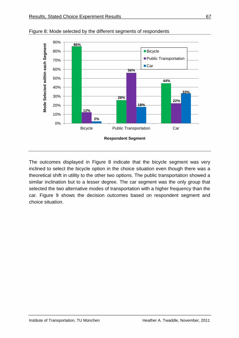
Results, Stated Choice Experiment Results 67
Institute of Transportation, TU München Heather A. Twaddle, November, 2011
Figure 8: Mode selected by the different segments of respondents
The outcomes displayed in Figure 8 indicate that the bicycle segment was very
inclined to select the bicycle option in the choice situation even though there was a
theoretical shift in utility to the other two options. The public transportation showed a
similar inclination but to a lesser degree. The car segment was the only group that
selected the two alternative modes of transportation with a higher frequency than the
car. Figure 9 shows the decision outcomes based on respondent segment and
choice situation.
86%
26%
44%
12%
56%
22%
2%
18%
33%
0%
10%
20%
30%
40%
50%
60%
70%
80%
90%
Bicycle Public Transportation Car
Mo
de S
ele
cte
d w
ith
in e
ach
Seg
men
t
Respondent Segment
Bicycle
Public Transportation
Car
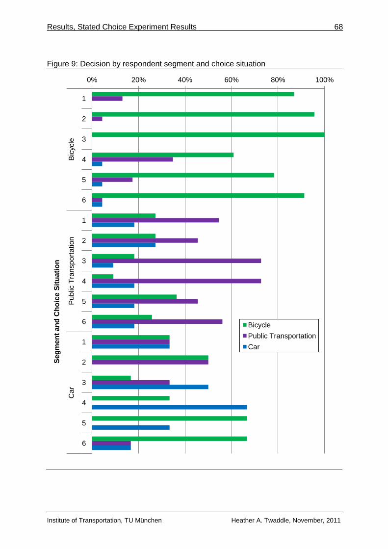
Results, Stated Choice Experiment Results 68
Institute of Transportation, TU München Heather A. Twaddle, November, 2011
Figure 9: Decision by respondent segment and choice situation
0% 20% 40% 60% 80% 100%
1
2
3
4
5
6
1
2
3
4
5
6
1
2
3
4
5
6
Bic
ycle
P
ub
lic T
ran
sp
ort
atio
n
Ca
r
Se
gm
en
t a
nd
Ch
oic
e S
itu
ati
on
Bicycle
Public Transportation
Car
Results, Stated Choice Experiment Results 69
Institute of Transportation, TU München Heather A. Twaddle, November, 2011
Although the estimation of the β parameters was not included in the scope of this
thesis, Figure 9 is useful in determining the choice situations in which utility balance
was achieved. According to Figure 9, a utility balance was best achieved for the car
segment, particularly for choice situations 1 and 3. The utility balance for the public
transportation also appears to be acceptable. However, the utility for the bicycle
segment is quite unbalanced, with the bicycle dominating the choice situation in all
six of the situation.
The respondents were given the opportunity to leave a comment on any of the pages
the survey. Three of the respondents chose to do so and their comments have been
included below:
Die Änderungen der Fahrzeiten/Preise/Wegbeschaffung sollte man besser
darstellen, sonst ist das ja auch ein Suchspiel... Außerdem ist es ein großer
Unterschied ob man neben 2 Fahrspuren und Parkstreifen noch mit dem Rad
unterwegs ist (Orleansstraße nördlich) oder ob da keiner parkt, 3 Spuren da
sind und eine breite rot lackierte Fahrradspur existiert (Orleansstraße südlich).
Das sollte man differenziert betrachten.
(The changes in travel time/price/trip characteristics should be organized
better. Otherwise it is a game of searching for the values...In addition, there is
a big different travelling with a bicycle on a street with two driving lanes and a
parking lane (Orleansstraße north) or if there is no parking, three lanes and a
wide, red-marked bicycle lane (Orleansstraße south). This should be
differentiated.)
It's hard to beat a bike on a 2 km ride with almost no traffic, no matter how the
prices or roads change
... die Entscheidung, ob Fahrrad oder Öffentliche Verkehrsmittel ist manchmal
nicht ganz leicht gefallen, beide sind für mich recht gleichwertig /
gleichberechtigt. Entscheidend ist vielmehr oft bspw die Wetterlage oder die
Kleidung (mit Rock und Blazer radelt sichs nicht so gut)
(... the choice between the bicycle and public transportation is sometimes not
easy to make because they are quite equal for me. Often, the decisive factor
is weather or clothing (it is not so easy to cycle in a skirt and blazer).
Discussion, Sample Recruitment 70
Institute of Transportation, TU München Heather A. Twaddle, November, 2011
5. DISCUSSION
The following section consists of a discussion about the sample recruitment, the
design of the time-use-travel diary and the stated choice experiment, and about the
outcomes from both data collection methods. The methodology used to create an
individualized stated choice experiment from reference scenarios is qualitatively
analysed. The distribution and collection methods are also discussed.
5.1. Sample Recruitment
The method used to recruit participants to this research project was not particularly
successful. Although the target of 50 test survey participants was nearly reached, the
systematic approach of mass emailing survey invitations to colleagues, friends and
family, as well as mailing survey invitations to 500 commercially purchased
addresses did not yield this result. After being sent the survey invitation, many
friends and family members were contacted personally or by phone and were asked
directly if they would take part in the survey and if they could provide their mailing
address. An overly long invitation letter, a complicated sign-up process and an
inconvenient timeframe for participation are all thought to have negatively affected
survey participation.
The original invitation letter, which was sent out as an email attachment to friends
and family of the „Radverkehr heute und morgen‟ research team and was posted to
the 500 commercially provided addresses, was two pages long and contained very
specific participation information. This version of the letter is attached in Appendix B.
The length of the letter, as well as the level of detail of the information could be one
reason for the low response to the invitation. It may also be a reason that the people
who did respond to the invitation by email often neglected to include their mailing
address in the email. Several features of the survey invitation letter were improved to
encourage a larger and more representative sample of people to take part in the
survey. The letter was shortened, reorganized, reformatted and simplified in an
attempt to make it more manageable and less daunting for potential survey
participants. The improved invitation letter (see Appendix B) is one page long, does
not contain any banking information for the research department, focuses on the
participation incentive and provides only the necessary details. Additionally, the
excessive focus on bicycle transportation in the original invitation letter may have
discouraged non-cyclists or people who bicycle infrequently from participating in the
survey. In order to attract a more representative sample of respondents, the
improved invitation letter presents the research project as an investigation of model

Discussion, Sample Recruitment 71
Institute of Transportation, TU München Heather A. Twaddle, November, 2011
choice in Munich rather than a bicycle transportation study. Non-cyclists are explicitly
invited to participate in the survey.
In addition to the long, detailed formation letter, the complicated sign-up process
may have exacerbated the low participation rate. Upon reading the information letter,
potential survey participants were asked to send an email containing their mailing
address to the email address set up for the research project. Instead of sending the
invitation letter as an attachment to an email or as a hard copy, it may be preferable
to put the text of the letter directly in the body of an email or to contact potential
participants by phone rather than by mail. It may also be worthwhile to explore
automatic means of asking people for their mailing address when they email back
their intention to take part in the survey. Another possibility is to abandon the use of
hard copy time-use-travel diaries in favour of digital diaries that can be filled out
online. This would eliminate the need for collecting mailing addresses from the
respondents and would streamline the sign-up process.
Finally, the timing of the distribution of the invitation letters and time-use-travel
diaries is thought to have negatively affected the survey response rate. The summer
school vacation in Bavaria took place between July 30th and September 12th, 2011,
while the lecture free period at TU München took place from July 30th to October
17th, 2011. Many students and families are not in Munich during this time, and if they
are in Munich, may not follow a normal schedule. If the survey was to be conducted
using a larger sample of respondents, it would be preferable to carry out the survey
during a time of year when there are no conflicting holidays or celebrations. In
addition, it may be advantageous to conduct the survey in two or more waves at
different points in the year. This would make it possible to observe differences in
bicycling behaviour under different seasonal conditions (weather, scheduling
difference due to holiday, etc.).
A survey hotline was made available to all participants for the entire duration of the
survey (between August 22nd and October 30th, 2011). During this time, none of the
participants called the hotline. This may be due to the fact that the majority of the
survey participants were friends or family of the „Radverkehr heute und morgen‟
team and could ask in person if they had any difficulty with the diary or online
questionnaire. However, it may also be that the information documents provided with
the time-use-travel diaries and the information buttons offered in the online
questionnaire provide adequate information for the respondents and a survey hotline
is not necessary.
Discussion, Stated Choice Experiment 72
Institute of Transportation, TU München Heather A. Twaddle, November, 2011
5.2. Time-Use-Travel Diary
One of the objectives of this research project was to design and test a combined
time-use-travel diary that would capitalize on the advantages of both time-use and
travel diaries while avoiding the respective pitfalls of each. Although the majority of
the survey respondents filled out the diary without many problems, there were some
areas that seemed to cause some confusion among the respondents.
Firstly, three of the 48 respondents did not enter any locality information, or if they
did, did not specify addresses, but referred to places such as „home‟, „work‟, „store‟,
etc.. The lack of this information made it impossible to estimate the characteristics of
the alternative modes of transportation, which as a result, eliminated these three
respondents from the SP portion of the survey. In order to reduce the number of
respondents who failed to enter address information in a subsequent survey, the
heading in the column in the diary could be changed from „Verkehrsmittel / Ort der
Aktivität‟ to „Verkehrsmittel / Adresse der Aktivität‟ (from „Mode of transportation /
Location of activity‟ to „Mode of transportation / Address of activity‟). It could also be
more clearly stated in the instructions that the address information is critical to the
analysis of the data. However, one possible reason for neglecting to enter address
information is the wish to maintain privacy on the part of the respondent. If this is the
case, changing the heading of the column or rewording the instructions will not have
an impact on the number of respondents who do not give address information.
Secondly, there was a considerable amount of confusion among the participants as
to how to fill out the bicycle infrastructure used column. Many people filled out every
type of infrastructure that they used along their route, while others followed the
instructions and only indicated the type of infrastructure that they used for the largest
portion of their trip. However, because so many people indicated using more than
one type of infrastructure, the revealed preference data was coded in such a way
that all types of infrastructure used by the respondent could be recorded if they
indicated using more than one type of infrastructure. This was done by using a 0/1
variable for each type of infrastructure separately. Unfortunately, by using this
method, the detail of information collected from people who only entered the most
used infrastructure was somewhat lower. For this reason, it is recommended asking
all participants to mark down all the types of infrastructure that they used along their
route.
Several respondents commented on the overall lack of space in the time-use-travel
diary. The respondents had a particular problem with the height of the entry rows
and the width of the space provided for the „Main activity‟ and the „Secondary
Activity‟ columns. None of the respondents used both of the sides of paper that were
provided in the time-use-travel diary and the vast majority did not use all of the rows
Discussion, Stated Choice Experiment 73
Institute of Transportation, TU München Heather A. Twaddle, November, 2011
provided on the first page. If the survey was carried out using a larger sample of
respondents, it may be better to decrease the number of rows per page, increase the
height of the rows and omit the second page.
5.3. Stated Choice Experiment
The individualized stated choice experimental design constructed in the course of
this research project was only partially successful in collecting relevant choice data.
However, the outcomes of the stated choice experiment pre-test and the qualitative
analysis of these outcomes will make it possible to improve the experimental design,
and therefore increase the value of the resulting choice data, for future surveys.
The first issue with the experimental design was the apparent lack of utility balance
achieved in the choice situations. Although an attempt was made to encourage
respondents to select a different mode than selected for their reported trip by
concurrently increasing the overall utility of the alternative modes and decreasing the
utility of the mode used in the reported trip, a large portion of the respondents opted
for the same mode in the various choice situations. In total 69.6% of the choice
situations prompted the respondent to select the same mode as used in their
reference scenario. This tendency was particularly notable in the bicycle user group.
In 85.5% of the choice situations, the respondents who used a bicycle in their
reference scenario also selected the bicycle regardless of the offered alternatives
and conditions. Over half of the choice situations (56.1%) faced by the public
transportation segment respondents prompted the reselection of the public
transportation alternative. This finding suggests that the design for the bicycle
segment clearly was dominated by one alternative. The experimental design for the
public transportation segment was also dominated by one mode, but this domination
was less distinct. The domination of one alternative could be caused by a number of
faults in the experimental design of the choice situations.
Firstly, the attributes selected for all three modes included in the experimental design
may not have been the key influencing factors on mode choice. For bicyclists in
particular, the choice to travel by bicycle may not be based on the travel time of the
other modes or the cost of using these other modes. The choice to travel by bicycle
may be based more on the enjoyment of bicycling, the weather, the characteristics of
the activity, or any number of other attributes (trip, personal or latent) that were not
included in the experimental design. This was suggested by one of the comments
received from a survey participant. This participant noted that the utility offered by
the bicycle and public transportation alternatives are quite equal for them. The
selection between the two is influenced by daily factors such as the weather and the
clothing. This finding supports the claim made in previous research that the choice to
travel by bicycle may not be influenced as strongly by observable trip or personal
Discussion, Stated Choice Experiment 74
Institute of Transportation, TU München Heather A. Twaddle, November, 2011
characteristics as the choice to travel by other modes of transportation is (Heinen,
van Wee & Maat 2010; Johansson, Heldt & Johansson 2006).
Secondly, even if the attributes selected do significantly influence mode choice, the
outcome of the stated choice experiment may not reflect this significantly if the
attribute levels included in the experimental design are not properly selected to
concur with the indifference curves of the respondents. Because the pivot levels
used in the experimental design were adopted from research studies done by other
scientists and were not derived specifically for this research project, the pivot
percentages and the absolute value attribute levels very well may not have reflected
the indifference curves of the decision makers. A quantitative analysis of the results
would be necessary to estimate pivot percentages and absolute attribute levels that
would produce a better utility balance in the choice situations.
Although the experimental designs for the bicycle and public transportation
segments suffered from utility imbalance, the design for the car segment seemed to
produce fairly balanced results. This suggests that the attribute and attribute levels
included in the car segment experimental design may be adequate for the β
parameter estimations.
Overall the use of an efficient design process was deemed to be appropriate.
However, the true statistical outcomes of this decision cannot be assessed until the
data is used to estimate β parameters in a model. The attrition rate was not found to
be a significant problem because of the relatively high secondary response rate of
93%.
One drawback of the survey implementation process was that it was not possible to
incorporate information collected in the personal questionnaire in the design of the
stated choice experiments. For example, each of the respondents was presented
with a choice situation that included all three mode alternatives. However, if
information was available beforehand about bicycle and car ownership, it would be
possible to remove either the car or bicycle alternative if the respondent did not own
a car or bicycle. Furthermore, because the stated choice experiment was presented
to the respondent after the questions in the personal questionnaire that enquired
about bicycle and car ownership, the respondents may have viewed the subsequent
inclusion of these options as unrealistic if they did not own a car or bicycle. Two of
the respondents commented on this flaw.
As a quantitative analysis of the data collected in the stated choice experiment was
not included in the scope of this project, it is not possible to determine conclusively if
the selected attributes had a significant influence on the decision of the respondent.
The next step in this research project would be the estimation of the β parameters
from the data collected. These parameters could then replace the parameters that
were adopted from previous research and used in the efficient design of this choice
Discussion, Stated Choice Experiment 75
Institute of Transportation, TU München Heather A. Twaddle, November, 2011
experiment. By implementing more precise β parameters in the efficient design,
better utility balance would be built into the choice situations.
A further recommendation for future work would be the use of focus groups to
identify important influencing factors on the choice to travel by bicycle. Because the
stated choice experiment was carried out online, it was not possible to ask the
respondents about the factors that influenced mode choice, specifically with regard
to cycling. The quantitative estimation of the influencing factors of bicycle
transportation is a very new area of research and as such no precedent has been set
as to the factors that have the most influence. As the number of factors that may
influence the choice to travel by bicycle is extremely large, it may be worthwhile to
carry out a number of stated choice experiments examining the influence of the
various factors separately.
Conclusions 76
Institute of Transportation, TU München Heather A. Twaddle, November, 2011
6. CONCLUSIONS
The methodology that was used to develop an individualized stated choice
experiment that investigated the choice to travel by bicycle was successful in some
areas but could be improved in others. The two-phase process that was used to
construct a stated choice experiment from a reference situation was found to be
cumbersome and work intensive.
The methods used to recruit the sample of participants needed for the pre-test of the
survey instruments was found to be very ineffective. An overly long invitation letter, a
complicated sign-up process and an inconvenient timeframe for participation are all
thought to have negatively affected survey participation. If such a survey were to be
carried out using a larger sample of respondents, it is advised that a different, more
streamlined method for recruitment be used. Additionally, because the completion of
both the time-use-travel diary and the online survey requires a significant amount of
time and effort on the part of the respondent, it may be necessary to introduce a
monetary incentive for participation if a large representative sample is needed.
The instrument used to collect the reference scenario information, the time-use-
travel diary was found to be an overall effective tool. The layout of the diary could be
amended to provide more room for the respondents to describe their trips and
activities. Better instructions and labelling for the „Verkehrsmittel/Ort der Aktivität‟
(Mode of transportation/Location of activity) could reduce the potential for
respondents to omit address information. It may be worthwhile to revise the columns
of the questionnaire regarding bicycle infrastructure used, as there was some
confusion amongst respondents as to how this should be filled out.
Although the time-use-travel diary instrument was adequate in collecting revealed
preference data, there is a potential to improve the entire survey process by
changing the paper and pencil format of the diary to an online version. The
digitalization of the time-use-travel diary would streamline the recruitment process
and would greatly diminish the work load of distributing and collecting the time-use-
travel diaries and then coding the data. The overall cost of the survey would also be
significantly reduced because there would be no need for printing or posting the
invitation letters or the survey documents.
The outcome of the stated choice experiment indicates that the attributes and
attribute levels that were included in the choice situations may need to be revised.
The experimental design of the choice situations that were presented to the segment
of respondents who had used a bicycle for their reported trip was dominated by the
bicycle option. This lack of utility balance is likely due to the fact that it is difficult to
identify the observable factors that influence the choice to bicycle. The results of this
Conclusions 77
Institute of Transportation, TU München Heather A. Twaddle, November, 2011
pre-test suggest that either insignificant attributes were included in the experimental
design for bicycle users, or the attribute levels did not reflect the indifference curves
of this sample. Focus groups could be used in future work to help identify the factors
that do indeed influence mode choice on the part of bicyclist. The utility balance of
the experimental design of the other two segments (car users and public
transportation users) appears to be much better. Still, the attribute levels and
experimental design could be improved to better estimate the β parameters of the
utility functions.
The method of building choice situations from a reference scenario familiar to the
respondent may be advantageous from a choice behaviour standpoint, but is difficult
to implement using the stated choice experiment building software that is currently
available. The process used in this project to code time-use-diaries, estimate the
reference scenarios for all the respondents and use this information to design
individualized stated choice experiment was complicated and work intensive. If such
a method were to be undertaken for a larger sample size, the workload would quickly
become unmanageable. For this reason, if such a technique were used for a larger
sample of respondents, it may be worthwhile to take several steps to simplify the
procedure. The reference scenarios could be aggregated based on trip length, which
would reduce the work load at the cost of slightly reducing the efficiency of the
experimental design. It is also recommended to implement a programming algorithm
to automatically perform several steps of the procedure.
There are several improvements that could be made to the procedure and
experimental design generated in this project to increase the statistical relevance of
the choice data collected from the stated choice experiment. However, the
methodology developed in this project provides a solid base for the development of
further stated choice experiments that investigate bicycle use.
List of Acronyms 78
Institute of Transportation, TU München Heather A. Twaddle, November, 2011
LIST OF ACRONYMS
AVC Asymptotic Variance Covariance
IIA Independence of Irrelevant Alternatives
IID Independent and Identically Distributed Terms
MLE Maximum Likelihood Estimation
MNL Multinomial Logit
MVV Münchner Verkehrs- und Tarifverbund
PuT Public Transportation
RP Revealed Preference
SC Stated Choice
Source of Reference 79
Institute of Transportation, TU München Heather A. Twaddle, November, 2011
SOURCE OF REFERENCE
Bibliography
Abraham, JE, McMillan, S, Brownlee, AT & Hunt, JD 2002, 'Investigation of Cycling
Sensitivities', Transportation Research Board Annual Conference, Transportation
Research Records, Washington D.C.
Ahern, AA & Tapley, N 2008, 'The use of stated preference techniques to model
modal choices on interurban trips in Ireland', Transportation Research Part A, vol 42,
pp. 15-27.
Aultman-Hall, LM 1996, 'Commuter Bicycle Route Choice: Analysis Of Major
Determinants And Safety Implications', Open Access Dissertations and Theses.,
Paper 2366.
Axhausen, KW & Polak, JW 1991, 'Choice of parking: Stated preference approach',
Transportation, vol 18, pp. 59-81.
Bamberg, S & Schmidt, P 1994, 'Auto oder Fahrrad: Empirischer Test einer
Handlungstheorie zur Erklärung der Verkehrsmittelwahl', Kölner Zeitschrift für
Soziologie und Soziopsychologie, pp. 80-102.
Ben-Akiva, ME & Lerman, S 1985, Discrete Choice Analysis: theory and application
to travel demand, MIT Press, Cambridge, Mass.
Bergström, A & Magnussen, R 2003, 'Potential of transferring car trips to bicycle
during winter', Transportation Research Part A, pp. 649-666.
Bördlein, E 2000, 'The Munich Bicycle Development Concept', Planungsreferat (City
Development Departement) München, Munich.
Buehler, R 2011, 'Determinants of transport mode: a comparison of Germany and
the USA', Journal of Transport Geography, vol 19, pp. 644-657.
Buehler, R & Pucher, J 2011, 'Cycling to work in 90 large American cities: new
evidence on the role of bike paths and lanes', Transportation.
ChoiceMetrics 2011, 'Ngene 1.1 User Manual and Reference Guide', ChoiceMetrics.
Dalla Rosa, J 2007, 'A Step Towards Sustainable Transportation Behaviour:
Understanding automobile ownership and mode choice through qualitative research',
University of Waterloo, Waterloo.
de Geus, B 2007, 'Cycling to work: Psychosocial and environmental factors
associated with cycling and the effect of cycling on fitness and health indexes in an

Source of Reference 80
Institute of Transportation, TU München Heather A. Twaddle, November, 2011
untrained working population', Doctoral dissertation, Vrije Universiteit Brussel,
Brussels.
dell‟Olio, L, Ibeas, A, Cecín, P & Francesco, D 2011, 'Willingness to pay for
improving service quality in a multimodal area', Transportation Research Part C, pp.
1060-1070.
Dickinson, JE, Kingham, S, Copsey, S & Hougie, DJP 2003, 'Employer travel plans,
cycling and gender: will travel plan measures improve the outlook for cycling to work
in the UK?', Transportation Research Part D, pp. 53-67.
Dill, J 2009, 'Bicycling for Transportation and Health: The Role of Infrastructure',
Journal of Public Health Policy, vol 30, pp. 95-110.
Dill, J & Carr, T 2003, 'Bicycle Commuting and Facilities in Major U.S. Cities: If You
Build Them, Commuters Will Use Them', Transportation Research Record: Journal
of the Transportation Research Board, pp. 116-123.
Dill, J & Voros, K 2007, 'Factors Affecting Bicycle Demand: Initial Survey Findings
from the Portland Region', Transportation Research Board, Washington DC.
Garrard, J, Rose, G & Kai Lo, S 2008, 'Promoting Transportation Cycling for Women:
The Role of Bicycle Infrastructure', Preventive Medicine, vol 46, pp. 55-59.
Handy, SL, Xing, Y & Buehler, TJ 2010, 'Factors associated with bicycle ownership
and use: a study of six small U.S cities', Transportation, vol 37, pp. 967-985.
Heinen, E, van Wee, B & Maat, K 2010, 'Commuting by Bicycle: An Overview of the
Literature', Transport Reviews, vol 30, no. 1, pp. 59-96.
Hensher, DA 1994, 'Stated preference analysis of travel choices: the state of
practice', Transportation, pp. 107-133.
Hensher, DA 2004, 'Identifying the influence of stated choice design dimensionality
on willingness to pay for travel time savings', Journal of Transport Economics and
Policy, p. 425–446.
Hensher, D & Greene, W 2003, 'The Mixed Logit Model: The State of Practice',
Transportation Research B, vol 30, pp. 133-176.
Hensher, DA & Johnson, L 1981, Applied Discrete Choice Modelling, Croom Helm,
London.
Hensher, DA, Rose, JM & Greene, WH 2005, Applied Choice Analysis: A Primer,
Cambridge University Press, Cambridge.
Horton, D, Rosen, P & Cox, P( 2007, Cycling and Society, Ashgate Publishing
Limited, Hampshire.
Hossain, MS, Hunt, JD & Wirasinghe, S 2010, 'Impact of Walking Distance on
Attractiveness of Transit Use', 12th WCTR 11-15, Portugal.
Source of Reference 81
Institute of Transportation, TU München Heather A. Twaddle, November, 2011
Hubert, J-P, Armoogum, J & Madre, J-L 2008, 'Immobility and Mobility seen through
trip-based versus time-use surveys', Transport Reviews, p. 641–658.
Hunt, JD & Abraham, JE 2007, 'Influences on bicycle use', Transportation, vol 34, p.
453–470.
Johansson, MV, Heldt, T & Johansson, P 2006, 'The effects of attitudes and
personality traits on mode choice', Transportation Research Part A: Policy and
Practice, vol 40, no. 6, pp. 507-525.
König, A & Axhausen, KW 2002, 'The reliability of the transportation system and its
Influence on the Choice Behaviour', 2nd Swiss Transport Research Conference,
Monte Verità.
Krizek, KJ 2006, 'Two Approaches to Valuing Some of Bicycle Facilities' Presumed
Benefits', Journal of the American Planning Association, vol 72, no. 3, pp. 309-320.
Krizek, KJ, Barnes, G & Thompson, K 2009, 'Analyzing the Effect of Bicycle Facilities
on Commute Mode Share over Time', Journal of Urban Planning and Development,
pp. 66-73.
Krizek, KJ, Johnson, PJ & Tilahun, N 2005, 'Gender Differences in Bicycling
Behavior and Facility Preferences', Research on Women's Issues in Transportation,
pp. 31-41.
Krizek, KJ & Roland, RW 2005, 'What is at the end of the road? Understanding
discontinuities of on-street bicycle lanes in urban settings', Transportation Research
Part D, vol 39, no. 10, pp. 55-68.
Kuhnimhof, T, Chlond, B & Huang, P-C 2010, 'Multimodal Travel Choices of
Bicyclists: Multday Data Analysis of Bicycle Use in Germany', Transportation
Research Record: Journal of the Transportation Research Board, No. 2190, pp. 19-
27.
Kuhnimhof, TG, Chlond, B & von der Ruhren, S 2006, 'Users of Transport Modes
and Multimodal Travel Behaviour: Steps Toward Understanding Traveler's Options
and Choices', Transportation Research RecordL Journal of the Transportation
Research Board, No. 1985, Transportation Research Board of the National
Academies, Washington DC.
Landeshauptstadt München 2010, 'Radverkehr in München', Perspektive München,
Munich.
Louviere, JJ, Hensher, DA & Swait, JD 2000, Stated Choice Methods: Analysis and
Application, Cambridge University Press, Cambridge.
Menghini, G, Carrasco, N, Schüssler, N & Axhausen, KW 2009, 'Route choice of
cyclists in Zurich: GPS-based discrete choice models', Arbeitsberichte Verkehrs- und
Raumplanung, Swiss Federal Institute of Technology Zurich, Zurich.

Source of Reference 82
Institute of Transportation, TU München Heather A. Twaddle, November, 2011
Nankervis, M 1999, 'The effect of weather and climate on bicycle commuting',
Transportation Research Part A, vol 33, pp. 417-431.
Nelson, AC & Allen, D 1997, 'If You Build Them, Commuters Will Use Them:
Association Between Bicycle Facilities and Bicycle Commuting', Transportation
Research Records, vol 1578, pp. 79-83.
Nobis, C 2007, 'Multimodality: Facets and Causes of Sustainable Behaviour',
Transportation Research Record: Journal of the Transportation Research Board, No.
2010, Transportation Reseach Board of the National Academies, Washington DC.
Ortúzar, JDD 2000, 'Modelling route and multimodal choices with revealed and
stated preference data', in JDD Ortúzar (ed.), Stated Preference Modelling
Techniques, 4th edn, PTRC Education and Research Services Ltd., Londres.
Ortúzar, JDD 2010, 'Methodological advancements in constructing designs and
understanding respondent behavior related to stated preference experiments',
Transportation Research, vol 44B, no. 6, pp. 717-719.
Ortúzar, JDD, Iacobelli, A & Valeze, C 2000, 'Estimating demand for a cycle-way
network', Transportation Research Part A, pp. 353-373.
Parkin, J, Ryley, TJ & Jones, TJ 2007, 'Barriers to cycling: an exploration of
quantitative analyses', in Civil Engineering: Book Chapters, UBIR: University of
Bolton Institutional Repository, Bolton.
Park, S & Kang, J 2008, 'Factors that influence walking and biking to the Station:
Modeling commuter rail users‟ access mode choice', Transportation Research Board
2008 Annual Meeting CD-ROM.
Pucher, J & Buehler, R 2006, 'Why Canadians cycle more than Americans: a
comparative analysis of bicycling trends and policies', Transport Policy, vol 13, no. 3,
pp. 265-279.
Pucher, J & Buehler, R 2008, 'Making Cycling Irresistible: Lessons from The
Netherlands, Denmark And Germany', Transport Reviews, vol 28, no. 4, pp. 495-
528.
Rose, JM & Bliemer, MCJ 2004, 'The design of stated choice experiments: the state
of practice', Working Paper, Institute for Transportation Studies, The University of
Sydney.
Rose, JM, Bliemer, MCJ, Hensher, DA & Collins, AT 2008, 'Designing efficient stated
choice experiments in the presence of reference alternatives', Transportation
Research Part B, p. 395–406.
Skinner, D & Rosen, P 2007, 'Hell is Other Cyclists: Rethinking Transport and
Identity', in Cycling and Society, Ashgate Publishing Limited, Hampshire.

Source of Reference 83
Institute of Transportation, TU München Heather A. Twaddle, November, 2011
Starmer, C 2000, 'Developments in non-expected utility theory: the hunt for a
descriptive theory of choice under risk', Journal of Economic Literature, p. 332–382.
Stinson, MA & Bhat, CR 2003, 'An Analysis of Commuter Bicyclist Route Choice
Using a Stated Preference Survey', Transportation Research Record: Journal of the
Transportation Research Board, vol 1828, pp. 107-115.
Stinson, MA & Bhat, CR 2004, 'Frequency of Bicycle Commuting: Internet-Based
Survey Analysis', Transportation Research Record , pp. 122-130.
Stinson, MA & Bhat, CR 2005, 'A Comparison of the Route Preferences of
Experienced and Inexperienced Bicycle Commuters', Transportation Research
Board, Washington DC.
Storchmann, K 2003, 'Externalities by Automobiles and Fare-Free Transit in
Germany - A Paradigm Shift?', Journal of Public Transportation, pp. 89-105.
Tilahun, NY 2005, 'Trails, lanes or traffic: Valuing bicycle facilities with an adaptive
stated preference survey', University of Minnesota, Minneapolis.
Twaddle, H, Hall, F & Bracic, B 2010, 'Latent Bicycle Commuting Demand and the
Effects of Gender on Commuter Cycling and Accident Rates', Paper submitted for
publication and presentation at the 89th Annual Meeting of the Transportation
Research Board, January 10-14, , Transportation Research Records, Washington,
D.C.
Vrtic, M, Schuessler, N, Erath, A & Axhausen, KW 2007, 'Design elements of road
pricing schemes and their acceptability', Transportation Research Board Annual
Meeting 2007 Paper #07-1548.
Vrtic, M, Schuessler, N, Erath, A & Axhausen, KW 2009, 'The impacts of road pricing
on route and mode choice behaviour', Journal of Choice Modelling, pp. 109-126.
Vuchic, VR 2005, Urban Transit Operations, Planning and Economics, Wiley, John &
Sons, Incorporated.
Vuchic, VR 2007, Urban Transit Systems and Technology, Wiley, John & Sons,
Incorporated.
Wardman, M, Tight, M & Page, M 2007, 'Factors influencing the propensity to cycle
to work', Transportation Research Part A, pp. 339-350.
Winters, M, Davidson, G, Kao, D & Teschke, K 2011, 'Motivators and deterrents of
bicycling: comparing influences on decisions to ride', Transportation, p. 153–168.
Zhou, Y, Outwater, ML & Proussaloglou, K 2005, 'Market Research on Gender-
Based Attitudinal Preferences and Travel Behavior.', Research on Women's Issues
in Transportation Report of a Conference: Transportation Research Board of
National Academies, Transportation Research Board.
Source of Reference 84
Institute of Transportation, TU München Heather A. Twaddle, November, 2011
Webliography
Allgemeiner Deutscher Automobil-Club e.V. 2011, ADAC Autokosten 2011, Munich,
viewed 30 August 2011,
<http://www.adac.de/_mm/pdf/autokostenuebersicht_47085.pdf>.
Garrard, J, Crawford, S & Hakman, N 2006, Revolutions for Women: Increasing
Women's Participation in Cycling for Recreating and Transport, viewed 24 July 2011,
<http://www.australianwomensport.com.au/images/Reports/victorian%20
research/Revolutions%20key%20findings%20A4.pdf>.
Globalpark AG 2011, Unipark, viewed 25 July 2011, < http://www.unipark.info/1-0-
online-befragungssoftware-fuer-studenten-und-universitaeten-unipark-home.htm>
Google maps 2011, Google Maps, viewed 5 July 2011, <http://maps.google.de/
maps?ct=reset>
Mobilität in Deutschland 2011, Mobilität in Deutschland, viewed 18 July 2011,
<http://www.mobilitaet-in-deutschland.de/index.htm>
Münchner Verkehrs- und Tarifverbund 2011, MVV Münchner Verkehrs- und
Tarifverbund, viewed 6 July 2011, <http://www.mvv-muenchen.de/>
Portal München Betriebs-GmbH & Co. 2011, münchen.de, Landeshauptstadt
München and Stadtwerke München GmbH, viewed 10 July 2011,
<http://www.muenchen.de/>
Statistisches Bundesland Deutschland 2010, Zeitbudgeterhebung, viewed 21 August
2011, <http://www.destatis.de/jetspeed/portal/cms/Sites/destatis/Internet/DE/Presse/
abisz/Zeitbudgeterhebung.psml>
List of Figures 85
Institute of Transportation, TU München Heather A. Twaddle, November, 2011
LIST OF FIGURES
Figure 1: Modal split in Munich, Germany in 2008 ..................................................... 3
Figure 2: Standard error as a function of sample size .............................................. 21
Figure 3: Flow chart for the modified Federov algorithm .......................................... 24
Figure 4: Structure of the Ngene code used to construct the experimental design .. 56
Figure 5: Example of an introduction page containing an introduction graphic ........ 58
Figure 6: Example of a choice situation as presented to a respondent .................... 59
Figure 7: Mode of transportation used for reported trip ............................................ 65
Figure 8: Mode selected by the different segments of respondents ......................... 67
Figure 9: Decision by respondent segment and choice situation ............................. 68
List of Tables 86
Institute of Transportation, TU München Heather A. Twaddle, November, 2011
LIST OF TABLES
Table 1: Coding of Alternative Modes of Transportation .......................................... 34
Table 2: Alternative, attribute and attribute level summary ....................................... 45
Table 3: Attribute levels based on mode reported in time-use-travel diary ............... 48
Table 4: Statistics of the attributes included in the stated choice experiment ........... 49
Table 5: Estimates of the β parameter values used for the car alternative in the
experimental design ................................................................................................. 51
Table 6: Estimates of the β parameter values used for the public transportation
alternative in the experimental design ...................................................................... 52
Table 7: Estimates of the β parameter values used for the public transportation
alternative in the experimental design ...................................................................... 53
Table 8: Experimental design for the car segment ................................................... 56
Table 9: Experimental design for the public transportation segment ........................ 57
Table 10: Experimental design for the bicycle segment ........................................... 57
Table 11: Summary of trips reported by respondents .............................................. 64
APPENDIX A – BICYCLE LITERATURE REVIEW TABLES
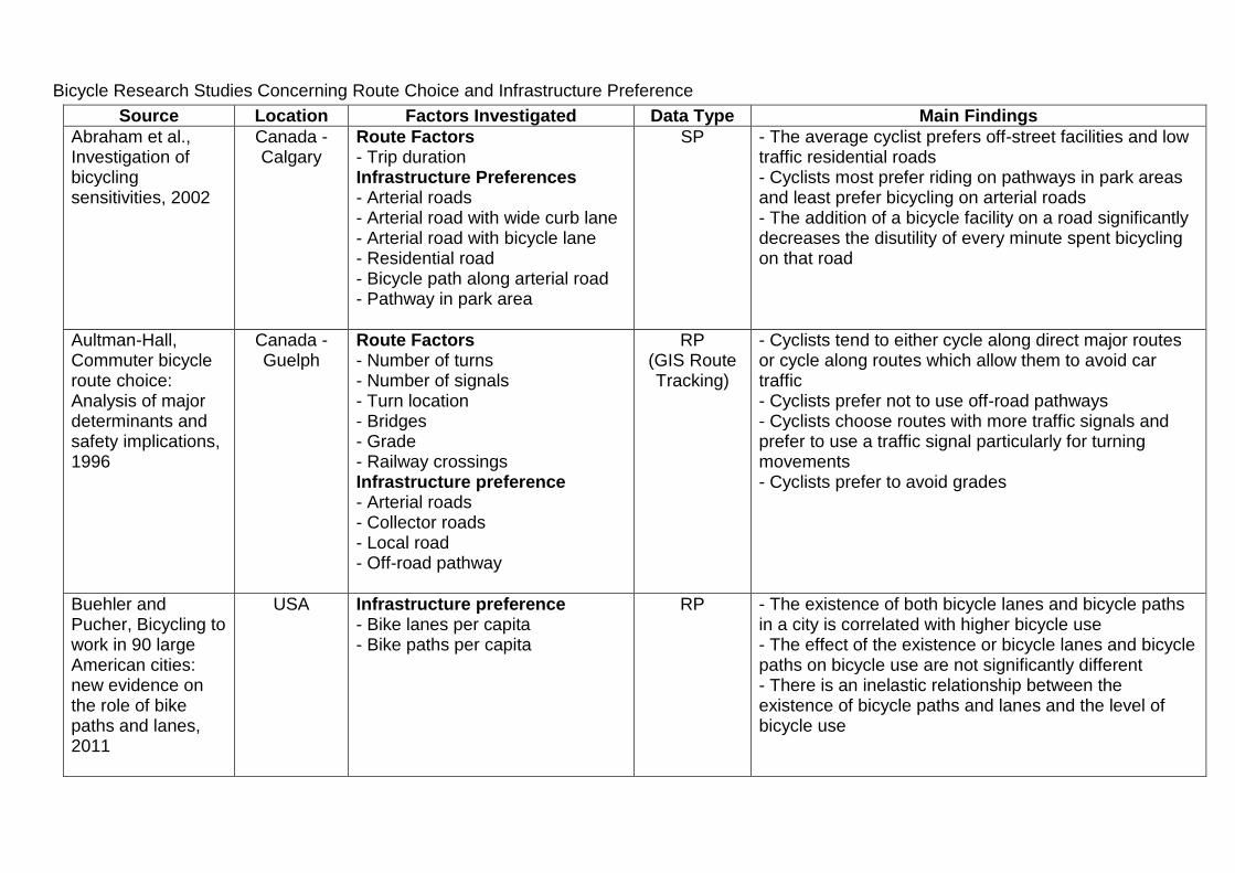
Bicycle Research Studies Concerning Route Choice and Infrastructure Preference
Source Location Factors Investigated Data Type Main Findings
Abraham et al., Investigation of bicycling sensitivities, 2002
Canada - Calgary
Route Factors - Trip duration Infrastructure Preferences - Arterial roads - Arterial road with wide curb lane - Arterial road with bicycle lane - Residential road - Bicycle path along arterial road - Pathway in park area
SP - The average cyclist prefers off-street facilities and low traffic residential roads - Cyclists most prefer riding on pathways in park areas and least prefer bicycling on arterial roads - The addition of a bicycle facility on a road significantly decreases the disutility of every minute spent bicycling on that road
Aultman-Hall, Commuter bicycle route choice: Analysis of major determinants and safety implications, 1996
Canada - Guelph
Route Factors - Number of turns - Number of signals - Turn location - Bridges - Grade - Railway crossings Infrastructure preference - Arterial roads - Collector roads - Local road - Off-road pathway
RP (GIS Route Tracking)
- Cyclists tend to either cycle along direct major routes or cycle along routes which allow them to avoid car traffic - Cyclists prefer not to use off-road pathways - Cyclists choose routes with more traffic signals and prefer to use a traffic signal particularly for turning movements - Cyclists prefer to avoid grades
Buehler and Pucher, Bicycling to work in 90 large American cities: new evidence on the role of bike paths and lanes, 2011
USA Infrastructure preference - Bike lanes per capita - Bike paths per capita
RP - The existence of both bicycle lanes and bicycle paths in a city is correlated with higher bicycle use - The effect of the existence or bicycle lanes and bicycle paths on bicycle use are not significantly different - There is an inelastic relationship between the existence of bicycle paths and lanes and the level of bicycle use
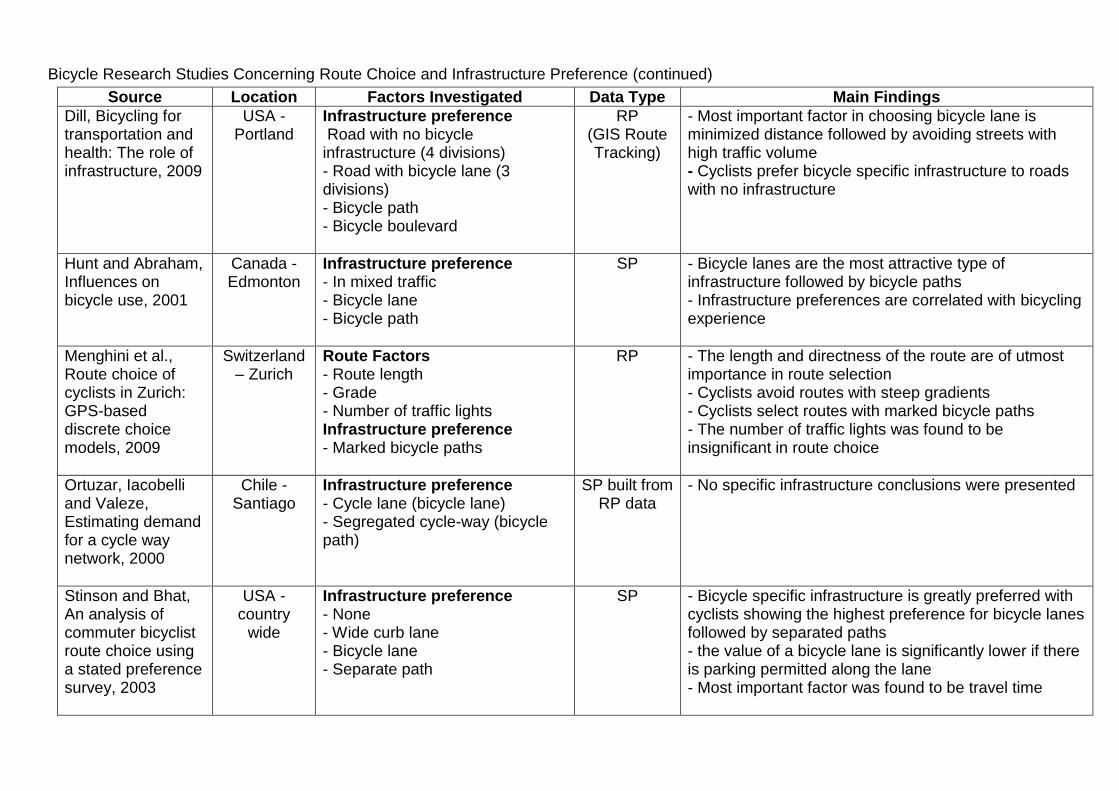
Bicycle Research Studies Concerning Route Choice and Infrastructure Preference (continued)
Source Location Factors Investigated Data Type Main Findings
Dill, Bicycling for transportation and health: The role of infrastructure, 2009
USA - Portland
Infrastructure preference Road with no bicycle infrastructure (4 divisions) - Road with bicycle lane (3 divisions) - Bicycle path - Bicycle boulevard
RP (GIS Route Tracking)
- Most important factor in choosing bicycle lane is minimized distance followed by avoiding streets with high traffic volume - Cyclists prefer bicycle specific infrastructure to roads with no infrastructure
Hunt and Abraham, Influences on bicycle use, 2001
Canada - Edmonton
Infrastructure preference - In mixed traffic - Bicycle lane - Bicycle path
SP - Bicycle lanes are the most attractive type of infrastructure followed by bicycle paths - Infrastructure preferences are correlated with bicycling experience
Menghini et al., Route choice of cyclists in Zurich: GPS-based discrete choice models, 2009
Switzerland – Zurich
Route Factors - Route length - Grade - Number of traffic lights Infrastructure preference - Marked bicycle paths
RP - The length and directness of the route are of utmost importance in route selection - Cyclists avoid routes with steep gradients - Cyclists select routes with marked bicycle paths - The number of traffic lights was found to be insignificant in route choice
Ortuzar, Iacobelli and Valeze, Estimating demand for a cycle way network, 2000
Chile - Santiago
Infrastructure preference - Cycle lane (bicycle lane) - Segregated cycle-way (bicycle path)
SP built from RP data
- No specific infrastructure conclusions were presented
Stinson and Bhat, An analysis of commuter bicyclist route choice using a stated preference survey, 2003
USA - country
wide
Infrastructure preference - None - Wide curb lane - Bicycle lane - Separate path
SP
- Bicycle specific infrastructure is greatly preferred with cyclists showing the highest preference for bicycle lanes followed by separated paths - the value of a bicycle lane is significantly lower if there is parking permitted along the lane - Most important factor was found to be travel time
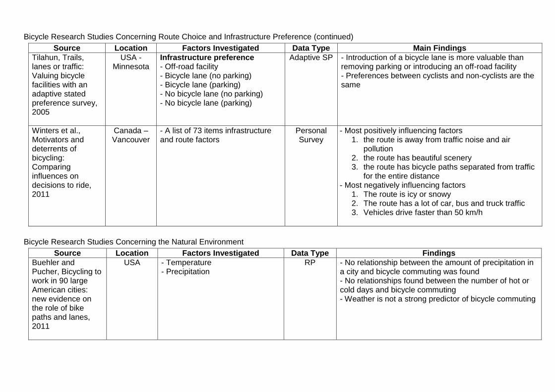
Bicycle Research Studies Concerning Route Choice and Infrastructure Preference (continued)
Source Location Factors Investigated Data Type Main Findings
Tilahun, Trails, lanes or traffic: Valuing bicycle facilities with an adaptive stated preference survey, 2005
USA - Minnesota
Infrastructure preference - Off-road facility - Bicycle lane (no parking) - Bicycle lane (parking) - No bicycle lane (no parking) - No bicycle lane (parking)
Adaptive SP - Introduction of a bicycle lane is more valuable than removing parking or introducing an off-road facility - Preferences between cyclists and non-cyclists are the same
Winters et al., Motivators and deterrents of bicycling: Comparing influences on decisions to ride, 2011
Canada – Vancouver
- A list of 73 items infrastructure and route factors
Personal Survey
- Most positively influencing factors 1. the route is away from traffic noise and air
pollution 2. the route has beautiful scenery 3. the route has bicycle paths separated from traffic
for the entire distance - Most negatively influencing factors
1. The route is icy or snowy 2. The route has a lot of car, bus and truck traffic 3. Vehicles drive faster than 50 km/h
Bicycle Research Studies Concerning the Natural Environment
Source Location Factors Investigated Data Type Findings
Buehler and Pucher, Bicycling to work in 90 large American cities: new evidence on the role of bike paths and lanes, 2011
USA - Temperature - Precipitation
RP - No relationship between the amount of precipitation in a city and bicycle commuting was found - No relationships found between the number of hot or cold days and bicycle commuting - Weather is not a strong predictor of bicycle commuting
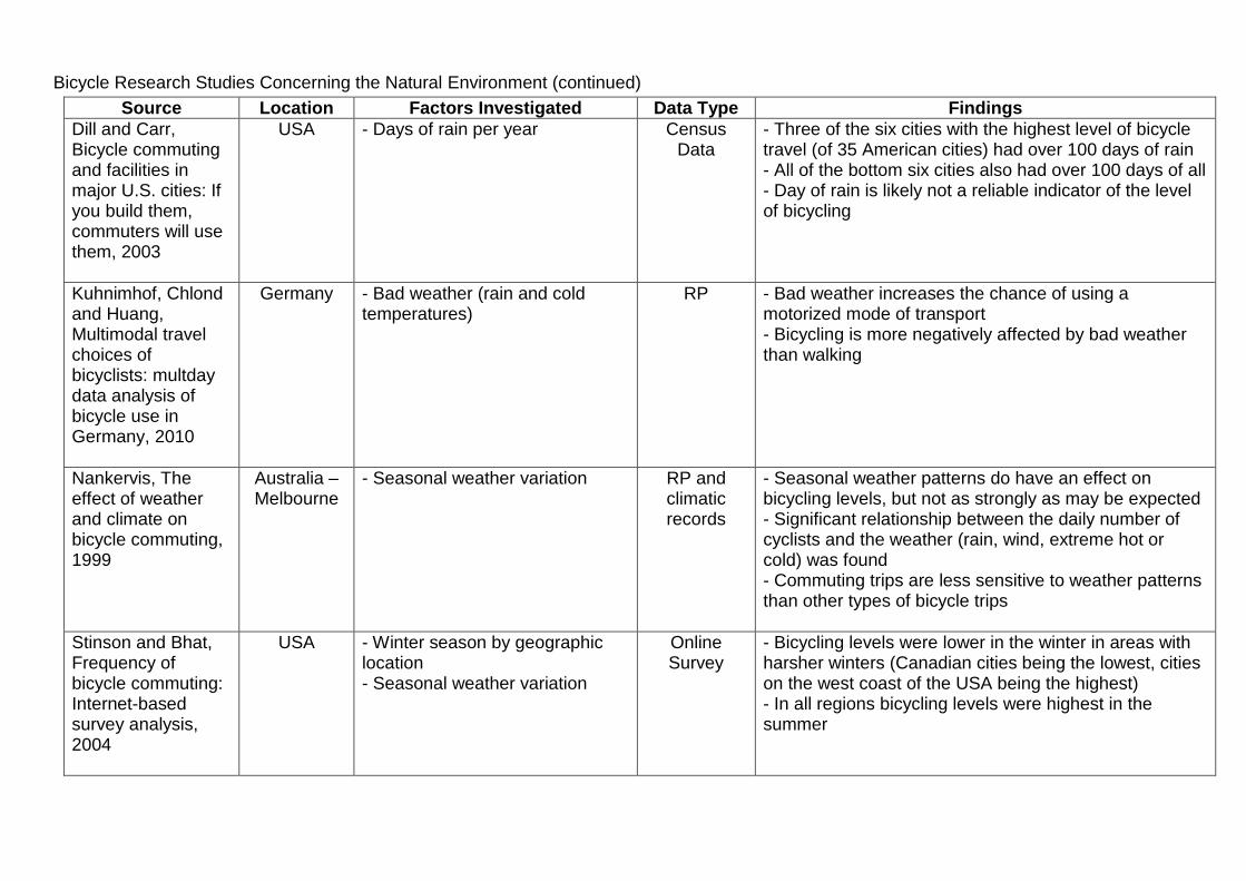
Bicycle Research Studies Concerning the Natural Environment (continued)
Source Location Factors Investigated Data Type Findings
Dill and Carr, Bicycle commuting and facilities in major U.S. cities: If you build them, commuters will use them, 2003
USA - Days of rain per year Census Data
- Three of the six cities with the highest level of bicycle travel (of 35 American cities) had over 100 days of rain - All of the bottom six cities also had over 100 days of all - Day of rain is likely not a reliable indicator of the level of bicycling
Kuhnimhof, Chlond and Huang, Multimodal travel choices of bicyclists: multday data analysis of bicycle use in Germany, 2010
Germany - Bad weather (rain and cold temperatures)
RP - Bad weather increases the chance of using a motorized mode of transport - Bicycling is more negatively affected by bad weather than walking
Nankervis, The effect of weather and climate on bicycle commuting, 1999
Australia – Melbourne
- Seasonal weather variation RP and climatic records
- Seasonal weather patterns do have an effect on bicycling levels, but not as strongly as may be expected - Significant relationship between the daily number of cyclists and the weather (rain, wind, extreme hot or cold) was found - Commuting trips are less sensitive to weather patterns than other types of bicycle trips
Stinson and Bhat, Frequency of bicycle commuting: Internet-based survey analysis, 2004
USA - Winter season by geographic location - Seasonal weather variation
Online Survey
- Bicycling levels were lower in the winter in areas with harsher winters (Canadian cities being the lowest, cities on the west coast of the USA being the highest) - In all regions bicycling levels were highest in the summer
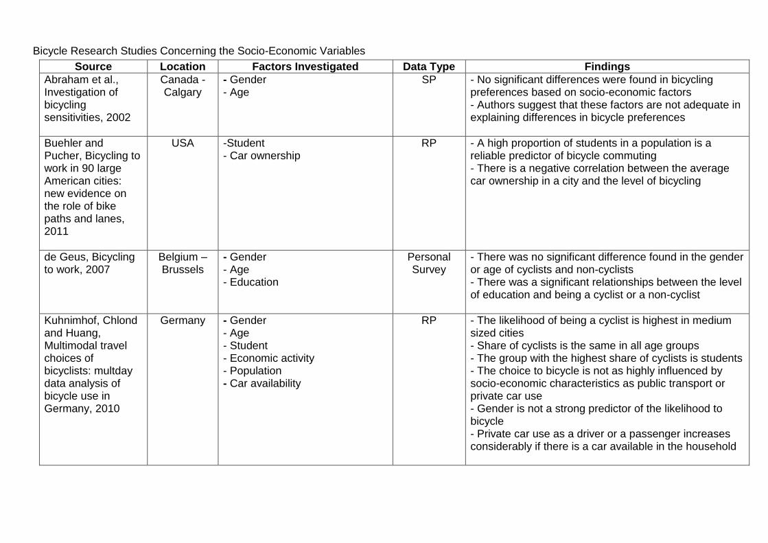
Bicycle Research Studies Concerning the Socio-Economic Variables
Source Location Factors Investigated Data Type Findings
Abraham et al., Investigation of bicycling sensitivities, 2002
Canada - Calgary
- Gender - Age
SP - No significant differences were found in bicycling preferences based on socio-economic factors - Authors suggest that these factors are not adequate in explaining differences in bicycle preferences
Buehler and Pucher, Bicycling to work in 90 large American cities: new evidence on the role of bike paths and lanes, 2011
USA -Student - Car ownership
RP - A high proportion of students in a population is a reliable predictor of bicycle commuting - There is a negative correlation between the average car ownership in a city and the level of bicycling
de Geus, Bicycling to work, 2007
Belgium – Brussels
- Gender - Age - Education
Personal Survey
- There was no significant difference found in the gender or age of cyclists and non-cyclists - There was a significant relationships between the level of education and being a cyclist or a non-cyclist
Kuhnimhof, Chlond and Huang, Multimodal travel choices of bicyclists: multday data analysis of bicycle use in Germany, 2010
Germany - Gender - Age - Student - Economic activity - Population - Car availability
RP - The likelihood of being a cyclist is highest in medium sized cities - Share of cyclists is the same in all age groups - The group with the highest share of cyclists is students - The choice to bicycle is not as highly influenced by socio-economic characteristics as public transport or private car use - Gender is not a strong predictor of the likelihood to bicycle - Private car use as a driver or a passenger increases considerably if there is a car available in the household
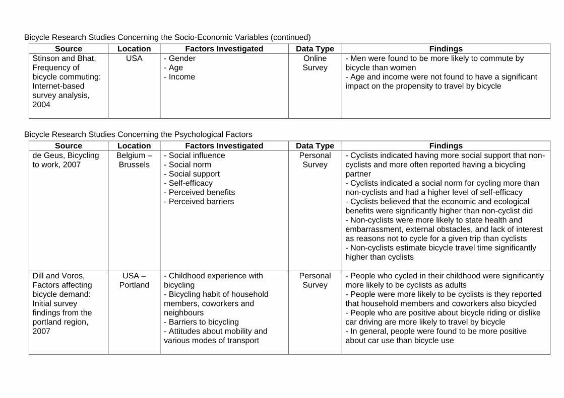
Bicycle Research Studies Concerning the Socio-Economic Variables (continued)
Source Location Factors Investigated Data Type Findings
Stinson and Bhat, Frequency of bicycle commuting: Internet-based survey analysis, 2004
USA - Gender - Age - Income
Online Survey
- Men were found to be more likely to commute by bicycle than women - Age and income were not found to have a significant impact on the propensity to travel by bicycle
Bicycle Research Studies Concerning the Psychological Factors
Source Location Factors Investigated Data Type Findings
de Geus, Bicycling to work, 2007
Belgium – Brussels
- Social influence - Social norm - Social support - Self-efficacy - Perceived benefits - Perceived barriers
Personal Survey
- Cyclists indicated having more social support that non-cyclists and more often reported having a bicycling partner - Cyclists indicated a social norm for cycling more than non-cyclists and had a higher level of self-efficacy - Cyclists believed that the economic and ecological benefits were significantly higher than non-cyclist did - Non-cyclists were more likely to state health and embarrassment, external obstacles, and lack of interest as reasons not to cycle for a given trip than cyclists - Non-cyclists estimate bicycle travel time significantly higher than cyclists
Dill and Voros, Factors affecting bicycle demand: Initial survey findings from the portland region, 2007
USA – Portland
- Childhood experience with bicycling - Bicycling habit of household members, coworkers and neighbours - Barriers to bicycling - Attitudes about mobility and various modes of transport
Personal Survey
- People who cycled in their childhood were significantly more likely to be cyclists as adults - People were more likely to be cyclists is they reported that household members and coworkers also bicycled - People who are positive about bicycle riding or dislike car driving are more likely to travel by bicycle - In general, people were found to be more positive about car use than bicycle use
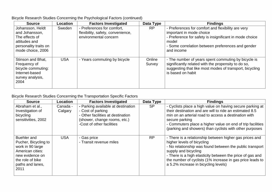
Bicycle Research Studies Concerning the Psychological Factors (continued)
Source Location Factors Investigated Data Type Findings
Johansson, Heldt and Johansson, The effects of attitudes and personality traits on mode choice, 2006
Sweden - Preferences for comfort, flexibility, safety, convenience, environmental concern
RP - Preferences for comfort and flexibility are very important in mode choice - Preference for safety is insignificant in mode choice model - Some correlation between preferences and gender and income
Stinson and Bhat, Frequency of bicycle commuting: Internet-based survey analysis, 2004
USA - Years commuting by bicycle Online Survey
- The number of years spent commuting by bicycle is significantly related with the propensity to do so, suggesting that like most modes of transport, bicycling is based on habit
Bicycle Research Studies Concerning the Transportation Specific Factors
Source Location Factors Investigated Data Type Findings
Abraham et al., Investigation of bicycling sensitivities, 2002
Canada - Calgary
- Parking available at destination - Cost of parking - Other facilities at destination (shower, change rooms, etc.) -Cost of other facilities
SP - Cyclists place a high value on having secure parking at their destination and are will to ride an estimated 8.5 min on an arterial road to access a destination with secure parking - Commuters place a higher value on end of trip facilities (parking and showers) than cyclists with other purposes
Buehler and Pucher, Bicycling to work in 90 large American cities: new evidence on the role of bike paths and lanes, 2011
USA - Gas price - Transit revenue miles
RP - There is a relationship between higher gas prices and higher levels of bicycling - No relationship was found between the public transport supply and bicycling - There is a high elasticity between the price of gas and the number of cyclists (1% increase in gas price leads to a 5.2% increase in bicycling levels)
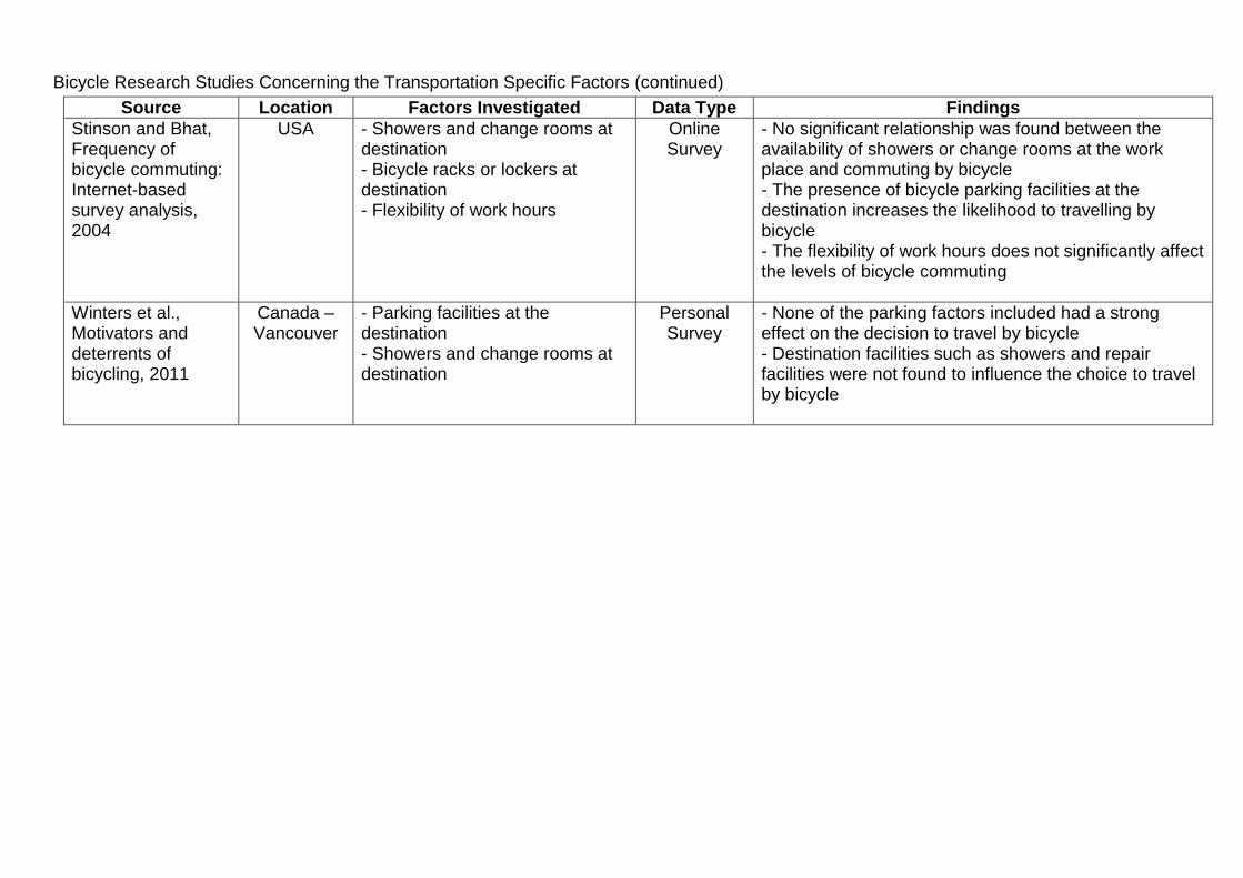
Bicycle Research Studies Concerning the Transportation Specific Factors (continued)
Source Location Factors Investigated Data Type Findings
Stinson and Bhat, Frequency of bicycle commuting: Internet-based survey analysis, 2004
USA - Showers and change rooms at destination - Bicycle racks or lockers at destination - Flexibility of work hours
Online Survey
- No significant relationship was found between the availability of showers or change rooms at the work place and commuting by bicycle - The presence of bicycle parking facilities at the destination increases the likelihood to travelling by bicycle - The flexibility of work hours does not significantly affect the levels of bicycle commuting
Winters et al., Motivators and deterrents of bicycling, 2011
Canada – Vancouver
- Parking facilities at the destination - Showers and change rooms at destination
Personal Survey
- None of the parking factors included had a strong effect on the decision to travel by bicycle - Destination facilities such as showers and repair facilities were not found to influence the choice to travel by bicycle

APPENDIX B - INVITATION LETTERS

Original German Invitation Letter

Seite 1
Technische Universität München
An alle potenzielle Teilnehmerinnen und Teilnehmer des Projektes „Radverkehr heute und morgen“
München, 1. August 2011
Sehr geehrte Damen und Herren, Sie nutzen Ihr Rad nicht, oder haben gar keines? Was würde Sie dazu veranlassen, es öfters zu nutzen oder ein Rad zu kaufen? Nutzen Sie ein Rad? Was kann die Stadt München für Sie als Radfahrer an der momentanen Verkehrssituation verbessern? Mit Ihrer Hilfe können wir daran arbeiten, Ihnen und anderen Radfahrern das Fahrradfahren angenehmer zu gestalten. Außerdem hoffen wir dadurch mehr Menschen zum Radfahren bewegen zu können. Wer sind wir? Eine Gruppe von jungen Verkehrs- und Mobilitätsforschern an der TU München. Wir führen im Rahmen einer Masterarbeit und ohne externe Finanzierung die Erhebung „Radverkehr heute und morgen“ durch. Ziel der Arbeit ist es, mehr über die Nutzung oder eben Nichtnutzung des Rades und die Gründe dafür zu erfahren. Was erwartet Sie: ein schriftliches Tagebuch, in welchem Sie kurz Ihre
Aktivitäten und Wege eines Tages niederschreiben, ein im Internet auszufüllender Online-Befragung, mit Fragen
zu Person und Haushalt und „Was-wäre-wenn Situationen“ wie zum Beispiel: würde sich Ihre Verkehrsmittelwahl ändern, wenn es an Ihrem Arbeitsplatz überdachte Abstellplätze für Fahrräder sowie Umkleidemöglichkeiten geben würde?
Technische Universität München
80290 München · Germany
Prof. Dr. Regine Gerike mobil.TUM – Projektgruppe
Mobilität & Verkehr
Lehrstuhl für Verkehrstechnik
Fakultät für Bauingenieur-
und Vermessungswesen
Arcisstraße 21
80333 München
Germany
Tel +49.89.289.28598
Fax +49.89.289.22333
www.mobil-tum.de
Bankverbindung:
Bayerische Landesbank
München
Konto-Nr.: 24 866
BLZ: 700 500 00
SWIFT-Code:
bylademm
IBAN-Nr.:
DE 10700500000000024866
Ust.-ID-Nr.:
DE811193231

Prof. Dr. Regine Gerike mobil.TUM – Projektgruppe
Mobilität & Verkehr
Lehrstuhl für Verkehrstechnik
Fakultät für Bauingenieur-
und Vermessungswesen
Seite 2
Technische Universität München
Wir bitten Sie herzlich, sich die Zeit zum Ausfüllen und Zurücksenden des Tagebuches sowie für die abschließende Online-Befragung zu nehmen. Unter allen Teilnehmern der Studie verlosen wir drei Gutscheine im Wert von je 50 € für das Sporthaus Schuster in München - damit Ihnen das Radfahren noch mehr Spaß macht. Wenn Sie an der Umfrage teilnehmen möchten, bitten wir Sie eine E-Mail mit Ihrer Anschrift an: [email protected] zu senden. Die benötigten Unterlagen für das Tagebuch werden Ihnen dann zeitnah zugesandt. Wir bitten Sie das Tagebuch an einem Werktag (vorzugsweise an einem Dienstag, Mittwoch oder Donnerstag) Ihrer Wahl zwischen Montag, den 22. August und Freitag, den 2. September auszufüllen. In dieser Zeit haben wir eine Hotline geschaltet. Tel.: +49 (0) 174 7142309 (Montag – Freitag,10.00 - 20.00 Uhr) Bitte schicken Sie das ausgefüllte Tagebuch in dem mitgesandten Rückumschlag zeitnah an uns zurück. Ein Link zu der abschließenden Online-Befragung wird Ihnen per E-Mail zugeschickt. Die Auslosung für die Gutscheine findet im Oktober statt. Wir arbeiten strikt nach den Vorschriften des Bundesdatenschutzgesetzes und allen anderen datenschutzrechtlichen Bestimmungen. Ihre Angaben werden in anonymisierter Form ausgewertet. Für Fragen stehen wir Ihnen unter der Email-Adresse [email protected] gern zur Verfügung. Herzlichen Dank für Ihre Unterstützung unserer Forschungsarbeit und die Teilnahme an dieser Untersuchung. Mit freundlichen Grüßen, Regine Gerike

Original English Invitation Letter
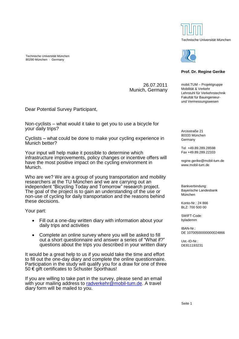
Seite 1
Technische Universität München
26.07.2011 Munich, Germany
Dear Potential Survey Participant, Non-cyclists – what would it take to get you to use a bicycle for your daily trips? Cyclists – what could be done to make your cycling experience in Munich better? Your input will help make it possible to determine which infrastructure improvements, policy changes or incentive offers will have the most positive impact on the cycling environment in Munich. Who are we? We are a group of young transportation and mobility researchers at the TU München and we are carrying out an independent “Bicycling Today and Tomorrow” research project. The goal of the project is to gain an understanding of the use or non-use of cycling for daily transportation and the reasons behind these decisions. Your part:
Fill out a one-day written diary with information about your daily trips and activities
Complete an online survey where you will be asked to fill out a short questionnaire and answer a series of “What if?” questions about the trips you described in your written diary
It would be a great help to us if you would take the time and effort to fill out the one-day diary and complete the online questionnaire. Participation in the study will qualify you for a draw for one of three 50 € gift certificates to Schuster Sporthaus! If you are willing to take part in the survey, please send an email with your mailing address to [email protected]. A travel diary form will be mailed to you.
Technische Universität München 80290 München · Germany
Prof. Dr. Regine Gerike mobil.TUM – Projektgruppe
Mobilität & Verkehr
Lehrstuhl für Verkehrstechnik
Fakultät für Bauingenieur-
und Vermessungswesen
Arcisstraße 21
80333 München
Germany
Tel +49.89.289.28598
Fax +49.89.289.22333
www.mobil-tum.de
Bankverbindung:
Bayerische Landesbank
München
Konto-Nr.: 24 866
BLZ: 700 500 00
SWIFT-Code:
bylademm
IBAN-Nr.:
DE 10700500000000024866
Ust.-ID-Nr.:
DE811193231

Prof. Dr. Regine Gerike mobil.TUM – Projektgruppe
Mobilität & Verkehr
Lehrstuhl für Verkehrstechnik
Fakultät für Bauingenieur-
und Vermessungswesen
Seite 2
Technische Universität München
You can complete the one-day travel diary on any work day between Monday August 22nd, 2011 and Friday September 2nd, 2011 (preferably on a Tuesday, Wednesday or Thursday). A hotline will be available during the survey (+49 (0) 174 7142309, Monday-Friday, 10:00 am - 8:00 pm). Completed travel diaries can be returned via mail in a provided envelope (as promptly as possible please!). A link to the online survey will then be emailed to you. The draw for the gift certificates will take place in October. We work strictly according to the provisions of the Federal Privacy Act and all other data protection regulations. Your information will be evaluated anonymously. Questions? Please contact us at [email protected]. Thank you for your support of our research project and your participation in the study! Sincerely, Regine Gerike

Revised German Invitation Letter

An alle potenziellen Teilnehmerinnen und Teilnehmer des Projektes „Radverkehr heute und morgen“
München, 04.10.2011 Hiermit laden wir Sie herzlich zur Teilnahme an unserer Umfrage zur Verkehrsmittelwahl in München ein. Wenn Sie die Umfrage ausgefüllt an uns zurücksenden, nehmen Sie an einer Verlosung teil, bei der Sie einen von fünf Gutscheinen für das Sporthaus Schuster in Höhe von 50 € gewinnen können. Der Schwerpunkt unserer Untersuchung liegt auf der Benutzung des Fahrrads und wie das Fahrrad als Verkehrsmittel in München besser unterstütz werden kann. Darüber hinaus sind wir interessiert Informationen von Einwohnern zu erhalten, die auch andere Verkehrsmittel verwenden. Auch als Nicht-Radfahrer sind Sie also herzlich dazu eingeladen an der Umfrage Teilzunehmen. Was erwartet Sie: ein schriftliches Tagebuch, in welchem Sie kurz Ihre
Aktivitäten und Wege eines Tages niederschreiben, ein im Internet auszufüllender Online-Befragung, mit
Fragen zu Person und Haushalt und „Was-wäre-wenn Situationen“ (das Ausfüllen des online-Fragebogens nimmt ca. 7- 10 Minuten in Anspruch.)
Wenn Sie an der Umfrage teilnehmen möchten, bitten wir Sie eine E-Mail mit Ihrer Anschrift an: [email protected] zu senden. Die benötigten Unterlagen für das Tagebuch werden Ihnen dann zeitnah zugesandt. Bitte schicken Sie das ausgefüllte Tagebuch in dem mitgesandten Rückumschlag zeitnah an uns zurück. Ein Link zu der abschließenden Online-Befragung wird Ihnen per E-Mail zugeschickt. Die Auslosung für die Gutscheine findet im Oktober statt. Für Fragen stehen wir Ihnen unter der Email-Adresse [email protected] gern zur Verfügung. Herzlichen Dank für Ihre Unterstützung unserer Forschungsarbeit und die Teilnahme an dieser Untersuchung. Mit freundlichen Grüßen, Regine Gerike
Prof. Dr. Regine Gerike mobil.TUM – Projektgruppe
Mobilität & Verkehr
Lehrstuhl für Verkehrstechnik
Fakultät für Bauingenieur-
und Vermessungswesen
Arcisstraße 21 80333 München Germany Tel +49.89.289.28598 Fax +49.89.289.22333 [email protected] www.mobil-tum.de
Technische Universität München

Revised English Invitation Letter

02.11.2011 Munich, Germany
Dear Potential Survey Participant,
You are invited to participate in our survey concerning transportation mode choice in Munich. By completing the survey, you will be entered in a draw for one of five gift certificates to Schuster Sporthaus (50 € each). The focus of our work is on bicycling and how this mode could be better supported in Munich. However, we are interested in gaining information from people using all modes of transport and so you do not have to be a cyclist to take part in this survey! What you can expect to do: Record (briefly) your trips and activities in a one day written
diary Complete an online survey where you will be asked to fill out a
short questionnaire and answer a series of “What if?” questions about the trips you described in your written diary
Please return your completed one day diary via mail in a provided envelope (as promptly as possible please!). A link to the online survey will then be emailed to you. The draw for the gift certificates will take place in October. Questions? Please contact us at [email protected]. Thank you for your support of our research project and your participation in the study! Best Regards, Regine Gerike
Prof. Dr. Regine Gerike mobil.TUM – Projektgruppe Mobilität
& Verkehr
Lehrstuhl für Verkehrstechnik
Fakultät für Bauingenieur-
und Vermessungswesen
Arcisstraße 21
80333 München
Germany
Tel +49.89.289.28598
Fax +49.89.289.22333
www.mobil-tum.de
Technische Universität München
APPENDIX C - TIME-USE-TRAVEL DIARY SURVEY - GERMAN
As distributed to survey participants
Please see Appendix D for an English translation

Liebe Befragungsteilnehmerinnen und -teilnehmer, mit dem Tagebuch halten Sie die wichtigste Unterlage zur Befragung „Radverkehr heute und morgen“ in den Händen. Nur durch Ihre genauen und sorgfältigen Angaben ist es möglich, die Aktivitäten und Wege von Personen darzustellen.
Wer soll ein Tagebuch führen?
Sie wurden per Zufallsauswahl ausgewählt. Ihre Teilnahme ist daher von hoher Wichtigkeit, um eine möglichst hohe Repräsentativität der Ergebnisse zu erreichen. Ihre Teilnahme ist selbstverständlich freiwillig.
Wann ist das Tagebuch zu führen?
Bitte füllen Sie das Tagebuch an einem Werktag (vorzugsweise an einem Dienstag, Mittwoch oder Donnerstag) Ihrer Wahl zwischen Montag, den 22. August und Freitag, den 2. September aus. Bitte wählen Sie wenn möglich einen typischen Tag. Außergewöhnliche Ereignisse können Sie auf Seite sechs des Tagebuchs benennen.
Was ist einzutragen?
In das Tagebuch sind alle Aktivitäten einzutragen, die mindestens 5 Minuten dauern. Die Beschreibung der Tätigkeit soll möglichst genau und ausführlich erfolgen. Achten Sie bitte darauf, dass unter einer Tätigkeit nicht nur eine körperliche Aktivität zu verstehen ist. So sind geistige Aktivitäten, wie z.B. Planung und Organisation des Haushalts (Überlegungen zum Einkauf, Planung einer Familienfeier, Tele-Shopping oder E-Banking), Gespräche oder Radio hören ebenfalls als Aktivität in das Tagebuch einzutragen.
Wege - Was ist beim Eintragen zurückgelegter Wege zu beachten?
Besonders wichtig ist die Erfassung aller Wege zwischen den Aktivitäten. Bitte tragen Sie auch kurze Wege und Wegeketten ein, z.B. zu Hause – Kind zur Kita gebracht – beim Bäcker eingekauft – Arbeit.
Am Ende des Tagebuchs haben wir noch einige ergänzende Fragen zu dem Aufzeichnungstag. Wir bitten Sie, auch diese Fragen zu beantworten.
Nach den einleitenden Seiten finden Sie Ausschnitte aus einem Mustertagebuch für eine Beispielsperson. Schauen Sie sich bitte das Beispiel an. Die Hinweise sollen Ihnen das Ausfüllen erleichtern.
Sollten Sie dennoch Probleme bei der Eintragung oder Zuordnung von Aktivitäten haben, wen- den Sie sich bitte mit Ihren Fragen an die Betreuer der Studie an der TU München ([email protected], Telefon +49 (0) 174 7142309 (Montag – Freitag, 10.00 - 20.00 Uhr)). Wir helfen Ihnen gerne weiter.
Ihre Angaben in diesem Tagebuch werden streng vertraulich behandelt. Die Eintragungen dienen ausschließlich der statistischen Auswertung. Alle mit der Befragung beauftragten Personen sind zur Verschwiegenheit verpflichtet. Sie können also volles Vertrauen gegenüber allen Beteiligten haben.
Herzlichen Dank für Ihre Teilnahme
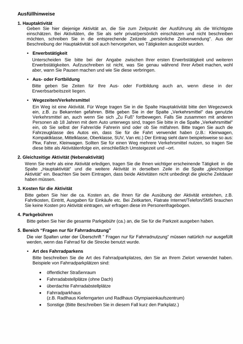
Ausfüllhinweise
1. Hauptaktivität Geben Sie hier diejenige Aktivität an, die Sie zum Zeitpunkt der Ausführung als die Wichtigste einschätzen. Bei Aktivitäten, die Sie als sehr privat/persönlich einschätzen und nicht beschreiben möchten, schreiben Sie in die entsprechende Zeitzeile „persönliche Zeitverwendung“. Aus der Beschreibung der Hauptaktivität soll auch hervorgehen, wo Tätigkeiten ausgeübt wurden.
• Erwerbstätigkeit
Unterscheiden Sie bitte bei der Angabe zwischen Ihrer ersten Erwerbstätigkeit und weiteren Erwerbstätigkeiten. Aufzuschreiben ist nicht, was Sie genau während Ihrer Arbeit machen, wohl aber, wann Sie Pausen machen und wie Sie diese verbringen.
• Aus- oder Fortbildung
Bitte geben Sie Zeiten für Ihre Aus- oder Fortbildung auch an, wenn diese in der Erwerbsarbeitszeit liegen.
• Wegezeiten/Verkehrsmittel
Ein Weg ist eine Aktivität. Für Wege tragen Sie in die Spalte Hauptaktivität bitte den Wegezweck ein, z.B. zu Bekannten gefahren. Bitte geben Sie in der Spalte „Verkehrsmittel“ das genutzte Verkehrsmittel an, auch wenn Sie sich „Zu Fuß“ fortbewegen. Falls Sie zusammen mit anderen Personen ab 18 Jahren mit dem Auto unterwegs sind, tragen Sie bitte in die Spalte „Verkehrsmittel“ ein, ob Sie selbst der Fahrer/die Fahrerin sind oder ob Sie mitfahren. Bitte tragen Sie auch die Fahrzeugklasse des Autos ein, dass Sie für die Fahrt verwendet haben (z.B.: Kleinwagen, Kompaktklasse, Mittelklasse, Oberklasse, SUV, Van etc.) Der Eintrag sieht dann beispielsweise so aus: Pkw, Fahrer, Kleinwagen. Sollten Sie für einen Weg mehrere Verkehrsmittel nutzen, so tragen Sie diese bitte als Aktivitätenfolge ein, einschließlich Umsteigezeit und –ort.
2. Gleichzeitige Aktivität (Nebenaktivität)
Wenn Sie mehr als eine Aktivität erledigen, tragen Sie die Ihnen wichtiger erscheinende Tätigkeit in die Spalte „Hauptaktivität“ und die weitere Aktivität in derselben Zeile in die Spalte „gleichzeitige Aktivität“ ein. Beachten Sie beim Eintragen, dass beide Aktivitäten nicht unbedingt die gleiche Zeitdauer haben müssen.
3. Kosten für die Aktivität
Bitte geben Sie hier die ca. Kosten an, die Ihnen für die Ausübung der Aktivität entstehen, z.B. Fahrtkosten, Eintritt, Ausgaben für Einkäufe etc. Bei Zeitkarten, Flatrate Internet/Telefon/SMS brauchen Sie keine Kosten pro Aktivität eintragen, wir erfragen diese im Personenfragebogen.
4. Parkgebühren
Bitte geben Sie hier die gesamte Parkgebühr (ca.) an, die Sie für die Parkzeit ausgeben haben.
5. Bereich “Fragen nur für Fahrradnutzung”
Die vier Spalten unter der Überschrift “ Fragen nur für Fahrradnutzung“ müssen natürlich nur ausgefüllt werden, wenn das Fahrrad für die Strecke benutzt wurde.
• Art des Fahrradparkens
Bitte beschreiben Sie die Art des Fahrradparkplatzes, den Sie an Ihrem Zielort verwendet haben. Beispiele von Fahrradparkplätzen sind:
öffentlicher Straßenraum
Fahrradabstellplätze (ohne Dach)
überdachte Fahrradabstellplätze
Fahrradparkhaus (z.B. Radlhaus Kieferngarten und Radlhaus Olympiaeinkaufszentrum)
Sonstige (Bitte Beschreiben Sie in diesem Fall kurz den Parkplatz.)
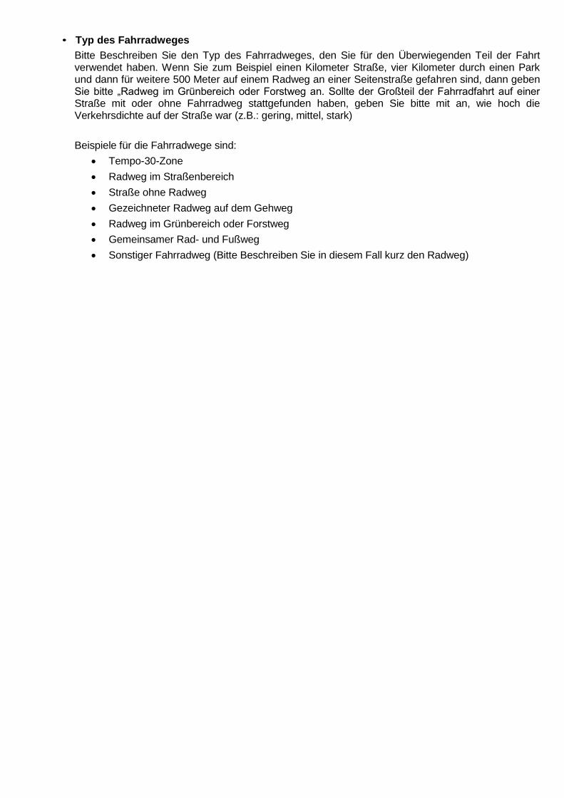
• Typ des Fahrradweges
Bitte Beschreiben Sie den Typ des Fahrradweges, den Sie für den Überwiegenden Teil der Fahrt verwendet haben. Wenn Sie zum Beispiel einen Kilometer Straße, vier Kilometer durch einen Park und dann für weitere 500 Meter auf einem Radweg an einer Seitenstraße gefahren sind, dann geben Sie bitte „Radweg im Grünbereich oder Forstweg an. Sollte der Großteil der Fahrradfahrt auf einer Straße mit oder ohne Fahrradweg stattgefunden haben, geben Sie bitte mit an, wie hoch die Verkehrsdichte auf der Straße war (z.B.: gering, mittel, stark)
Beispiele für die Fahrradwege sind:
Tempo-30-Zone
Radweg im Straßenbereich
Straße ohne Radweg
Gezeichneter Radweg auf dem Gehweg
Radweg im Grünbereich oder Forstweg
Gemeinsamer Rad- und Fußweg
Sonstiger Fahrradweg (Bitte Beschreiben Sie in diesem Fall kurz den Radweg)

HauptaktivitätVerkehrsmittel /
Ort der AktivitätGleichzeitige Aktivität Kosten
Park-
gebühren
Bewertung der
Fahrt/AktivitätVerfügbarkeit von
Duschen und/oder
Umkleidungsraum
am Zielort
Nutzung der
Duschen und/oder
Umkleidungsraum
am Zielort
��� ���(Ja/Nein/
weiß nicht)(Ja/Nein)
����� ����� ������ �� ������� ������������� ��� �
����� ����� � ����� ��� ������� �� �
����� ����� !�����"� ��� #�������� �$�� %
����� ���%� &���� �'��"� ��� �
���%� �(��� !����������)�� *"+��!�������,�-'�""$�� ������� �� �
�(��� ����� .�+��)/��"�� 0�"� ��$$���11���� ��� %
����� ����� 0�������� �$���� ���!�2 3�'�/���-��,�$$��� %
����� ����� ������ �-�&�$����� ������ ��� 3�'�/���-��,�$$��� ����� %
����� ����� �����"�� �4����$���� ���!�2 5�$��� ���� �
����� ����� .�+��)/��"�� 0�"� ��$$���11���� ��� �
����� ����� !������-�!� ����� *"+��!�������,�-'�""$�� ������� �� ���� �
����� �(�%� &'�� 5��-����'$��������� ��� ���"�� �� ���� %
�(�%� �(��� !�������&�'��-��" *"+��!�������,�-'�""$�� �
�(��� �1��� .� "���� .� "������������ ��� %1��� �
�1��� �1��� !���� ����6��� *"+��!�������,�-'�""$�� %
�1��� �1��� 7��)����� ���)� ��� ������������� ��� 8������� �����*� %
�1��� ����� �)� ��� ��� 3�'�/���-��*�� ��� %
����� ����� !����� �,� � !������ 3�'�/���-��*�� ��� � � #�� #�� �
����� ����� ,� �)�����-��*�� ��� 6�$$9+���)$:������� ��� ����� �
����� ����� !���� ����6��� !������ 3�'�/���-��*�� ��� ��3����� ������� � ;� #�� �
����� ����� *$� � ������� � ����$�� ������������� ��� %
����� ����� ���4������ ��� %
����� ����� &��$��� ��� �
Uhrzeit
bitte etwa im 5-Min.-Intervall angeben
Bitte immer nur eine Aktivität pro Zeile eintragen
Bitte geben Sie den genauen Ort der Aktivität an (Adresse), bzw.
das Verkehrsmittel für Wege
Bitte vergeben Sie Punkte:1 sehr unangenehm2 unangenehm3 neutral4 angenehm5 sehr angenehm
Bitte die wichtigste gleichzeitige Aktivität angeben
Bitte die allgemeinen Kosten für
die Aktivität angeben
(z.B.: 2,49 Euro)
Bitte die Kosten
für Parken(z.B.:
1,50 Euro)
Fragen nur für Fahrradnutzung
Typ des Fahrradweges
1 Tempo-30-Zone2 Radweg im Straßenbereich3 Straße ohne Radweg + Verkehrsdichte (gering, mittel, stark)
4 Gezeichneter Radweg auf Gehweg5 Radweg in Grünbereich / Forstweg6 Gemeinsamer Rad- und Fußweg7 Sonstiger (bitte beschreiben)
Art des Parkens
1 Öffentlicher Straßenraum 2 Fahrradabstellplätze (ohne Dach) 3 Überdachte Fahrradabstellplätze4 Fahrradparkhaus 5 Sonstige (bitte beschreiben)
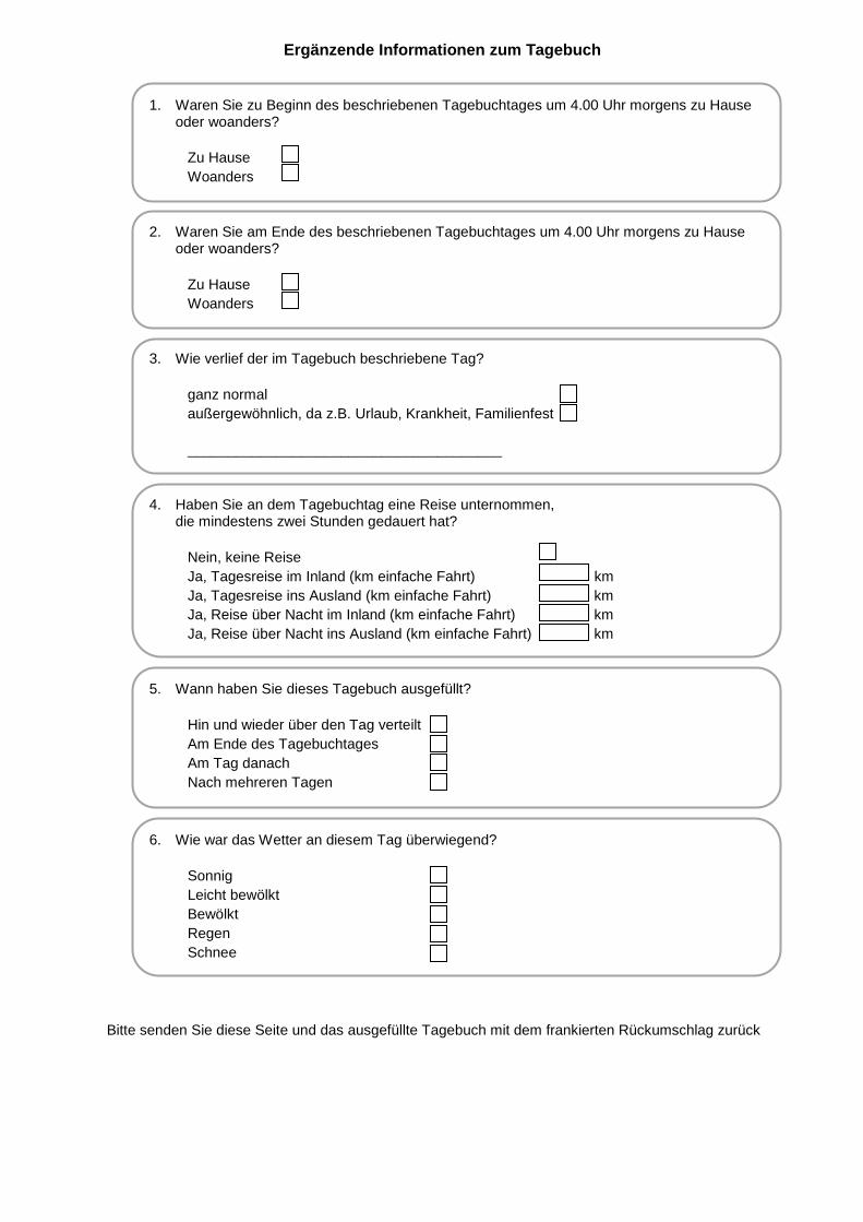
Ergänzende Informationen zum Tagebuch
1. Waren Sie zu Beginn des beschriebenen Tagebuchtages um 4.00 Uhr morgens zu Hause oder woanders?
Zu Hause
Woanders
2. Waren Sie am Ende des beschriebenen Tagebuchtages um 4.00 Uhr morgens zu Hause oder woanders?
Zu Hause
Woanders
3. Wie verlief der im Tagebuch beschriebene Tag?
ganz normal
außergewöhnlich, da z.B. Urlaub, Krankheit, Familienfest
_______________________________________
4. Haben Sie an dem Tagebuchtag eine Reise unternommen, die mindestens zwei Stunden gedauert hat?
Nein, keine Reise
Ja, Tagesreise im Inland (km einfache Fahrt) km
Ja, Tagesreise ins Ausland (km einfache Fahrt) km
Ja, Reise über Nacht im Inland (km einfache Fahrt) km
Ja, Reise über Nacht ins Ausland (km einfache Fahrt) km
5. Wann haben Sie dieses Tagebuch ausgefüllt?
Hin und wieder über den Tag verteilt
Am Ende des Tagebuchtages
Am Tag danach
Nach mehreren Tagen
6. Wie war das Wetter an diesem Tag überwiegend?
Sonnig
Leicht bewölkt
Bewölkt
Regen
Schnee
Bitte senden Sie diese Seite und das ausgefüllte Tagebuch mit dem frankierten Rückumschlag zurück

re
Raum für Anmerkungen (z.B. Hinweise für die weitere Bearbeitung, Schwierigkeiten beim Ausfüllen)
Erklärung zum Datenschutz und zur absoluten Vertraulichkeit Ihrer Angaben
Die Erhebung erfolgt durch die TU München im Rahmen der gleichnamigen Masterarbeit „Radverkehr heute und morgen“. Sie dient der Gewinnung statistischer Daten über Zeitverwendung und Mobilität privater Personen als Grundlage der in der zweiten Stufe der Befragung folgenden Online-Fragen zum Radverkehr. Die Zahl der angeschriebenen Personen liegt bei 500. Bei der Studie „Radverkehr heute und morgen“ trägt die TU München die datenschutzrechtlich Verantwortung. Wir arbeiten nach den gesetzlichen Bestimmungen des Datenschutzes. Die Ergebnisse der Studie werden ausschließlich in anonymisierter Form ohne Namen und Anschrift dargestellt. Nach Eingang Ihrer Unterlagen trennen wir Adresse und Fragenteil. Beide erhalten eine Codenummer. Ihre Angaben werden ohne Adresse und getrennt von den Adressen, d.h. in anonymisierter Form, gespeichert. Namen und Adressen verbleiben an der TU München, sind aber strikt getrennt von den Interviews und werden nur bis zum Abschluss der Studie aufbewahrt. Danach werden diese Angaben gelöscht. Sie können damit sicher sein: dass Ihr Name und Adresse nicht mit den Interviewdaten zusammen geführt werden. Niemand erfährt,
welche Angaben Sie persönlich gemacht haben, dass wir Ihren Namen und Anschrift nicht an Dritte weitergeben, dass wir keine Einzeldaten weitergeben, die einen Rückschluss auf Ihre Person zulassen, dass wir Ihre Angaben ausschließlich zu Forschungszwecken nutzen.
Wir bedanken uns für Ihr Vertrauen und Ihre Mitwirkung!
Radverkehr heute und morgen
Tagebuch
von: Bitte Namen eintragen
Email: Bitte eintragen, um den Link für die abschließende Befragung zu erhalten und an der Auslosung teilzunehmen.
TAG MONAT JAHR
Tagebuchtag 2 0 1 1
----------------------------------------------------------------------------------------------------------- Von der TU München auszufüllen
Eingangsdatum 2 0 1 1
Tag Monat Jahr
Haushalts-Nummer
Personen-Nummer

Hauptaktivität Verkehrsmittel /Ort der Aktivität Gleichzeitige Aktivität Kosten Park-
gebührenBewertung der Fahrt/Aktivität
Verfügbarkeit von Duschen und/oder Umkleidungsraum
am Zielort
Nutzung der Duschen und/oder Umkleidungsraum
am Zielort
von bis (Ja/Nein/weiß nicht) (Ja/Nein)
Uhrzeit
bitte etwa im 5-Min.-Intervall angeben
Bitte immer nur eine Aktivität pro Zeile eintragen
Bitte geben Sie den genauen Ort der Aktivität an (Adresse), bzw.
das Verkehrsmittel für Wege
Bitte vergeben Sie Punkte:1 sehr unangenehm2 unangenehm3 neutral4 angenehm5 sehr angenehm
Bitte die wichtigste gleichzeitige Aktivität angeben
Bitte die allgemeinen Kosten für
die Aktivität angeben
(z.B.: 2,49 Euro)
Bitte die Kosten
für Parken(z.B.:
1,50 Euro)
Fragen nur für Fahrradnutzung
Typ des Fahrradweges1 Tempo-30-Zone2 Radweg im Straßenbereich3 Straße ohne Radweg + Verkehrsdichte (gering, mittel, stark)4 Gezeichneter Radweg auf Gehweg5 Radweg in Grünbereich / Forstweg6 Gemeinsamer Rad- und Fußweg7 Sonstiger (bitte beschreiben)
Art des Parkens1 Öffentlicher Straßenraum 2 Fahrradabstellplätze (ohne Dach) 3 Überdachte Fahrradabstellplätze4 Fahrradparkhaus 5 Sonstige (bitte beschreiben)
Seite 1 von 2
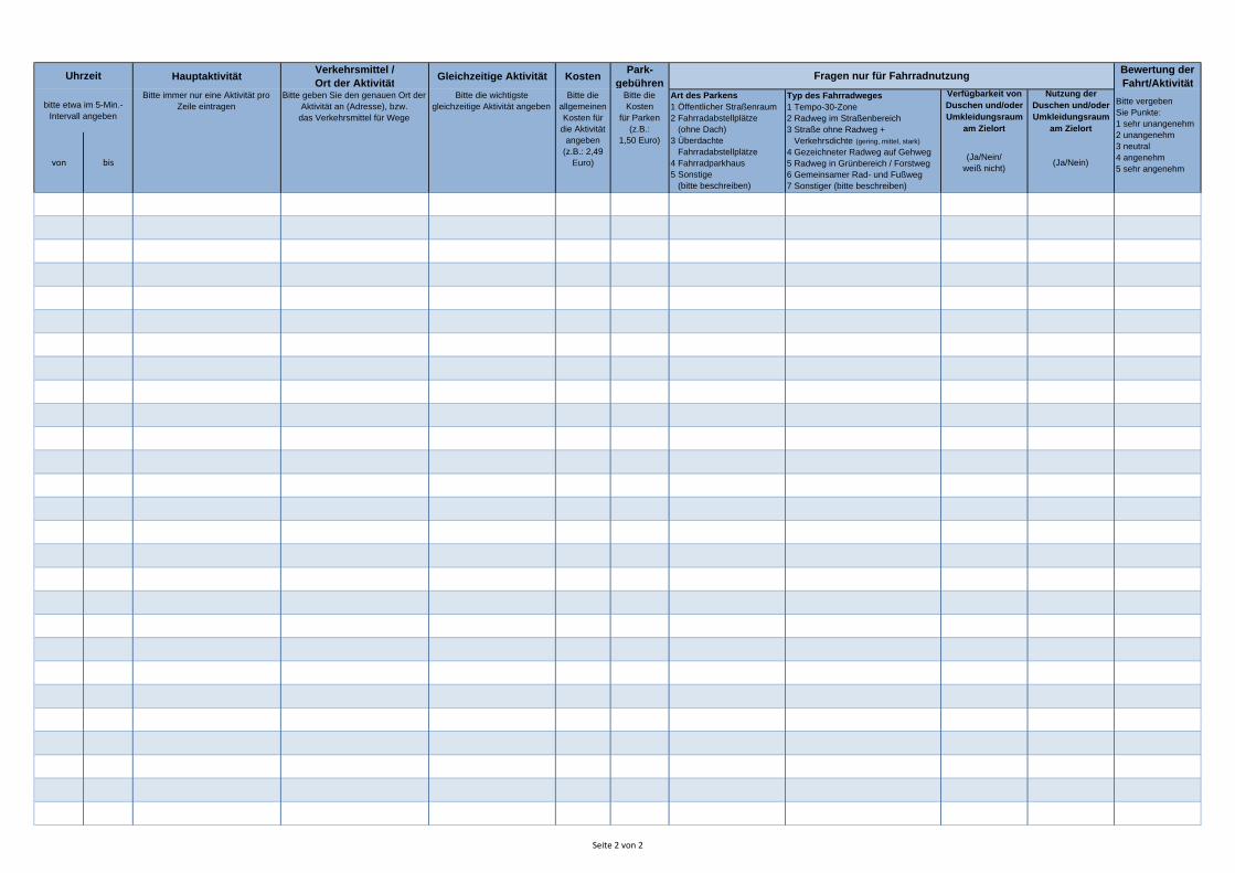
Hauptaktivität Verkehrsmittel /Ort der Aktivität Gleichzeitige Aktivität Kosten Park-
gebührenBewertung der Fahrt/Aktivität
Verfügbarkeit von Duschen und/oder Umkleidungsraum
am Zielort
Nutzung der Duschen und/oder Umkleidungsraum
am Zielort
von bis (Ja/Nein/weiß nicht) (Ja/Nein)
Uhrzeit
bitte etwa im 5-Min.-Intervall angeben
Bitte immer nur eine Aktivität pro Zeile eintragen
Bitte geben Sie den genauen Ort der Aktivität an (Adresse), bzw.
das Verkehrsmittel für Wege
Bitte vergeben Sie Punkte:1 sehr unangenehm2 unangenehm3 neutral4 angenehm5 sehr angenehm
Bitte die wichtigste gleichzeitige Aktivität angeben
Bitte die allgemeinen Kosten für
die Aktivität angeben
(z.B.: 2,49 Euro)
Bitte die Kosten
für Parken(z.B.:
1,50 Euro)
Fragen nur für Fahrradnutzung
Typ des Fahrradweges1 Tempo-30-Zone2 Radweg im Straßenbereich3 Straße ohne Radweg + Verkehrsdichte (gering, mittel, stark)4 Gezeichneter Radweg auf Gehweg5 Radweg in Grünbereich / Forstweg6 Gemeinsamer Rad- und Fußweg7 Sonstiger (bitte beschreiben)
Art des Parkens1 Öffentlicher Straßenraum 2 Fahrradabstellplätze (ohne Dach) 3 Überdachte Fahrradabstellplätze4 Fahrradparkhaus 5 Sonstige (bitte beschreiben)
Seite 2 von 2

APPENDIX D - ONLINE PERSONAL SURVEY AND STATED CHOICE EXPERIMENT
As distributed online to survey participants
Please see Appendix E and Appendix F for English translations
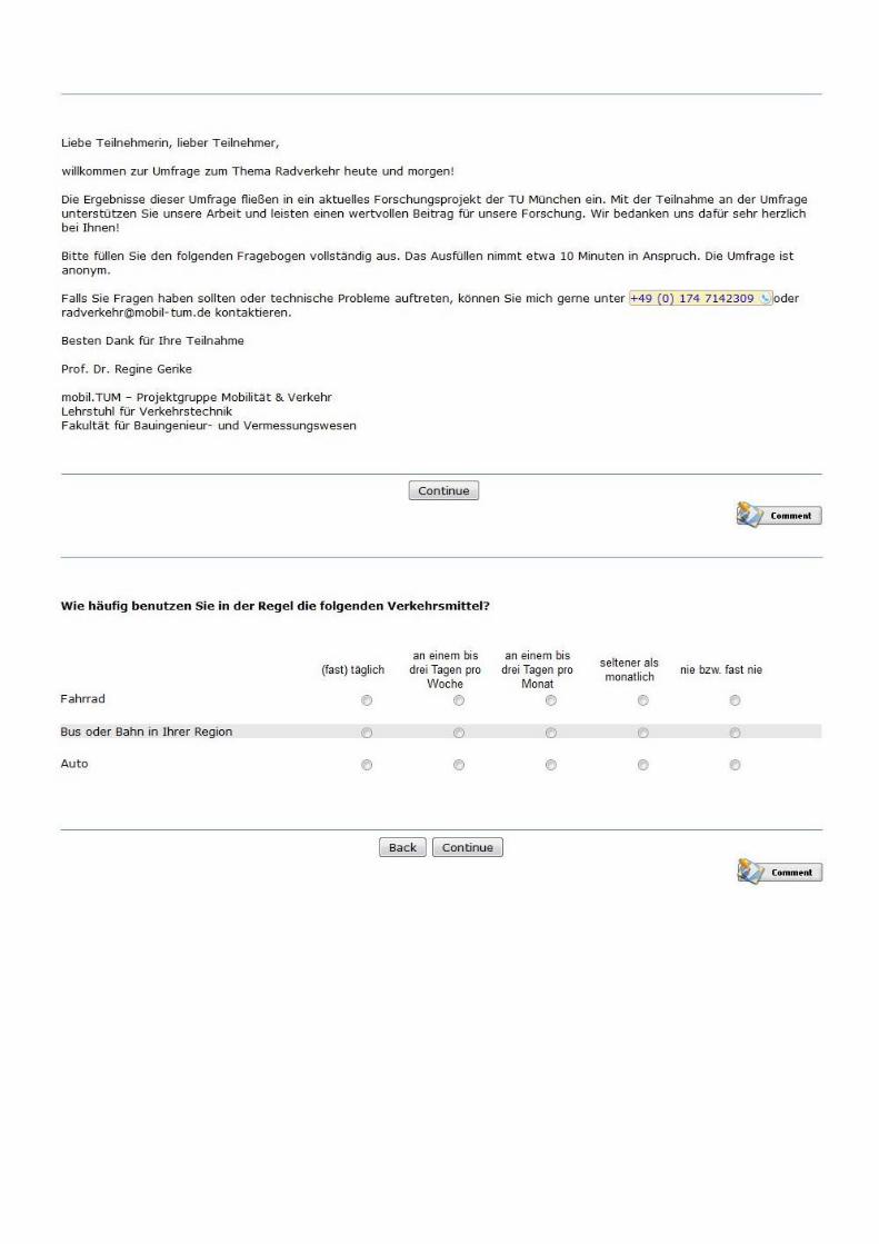
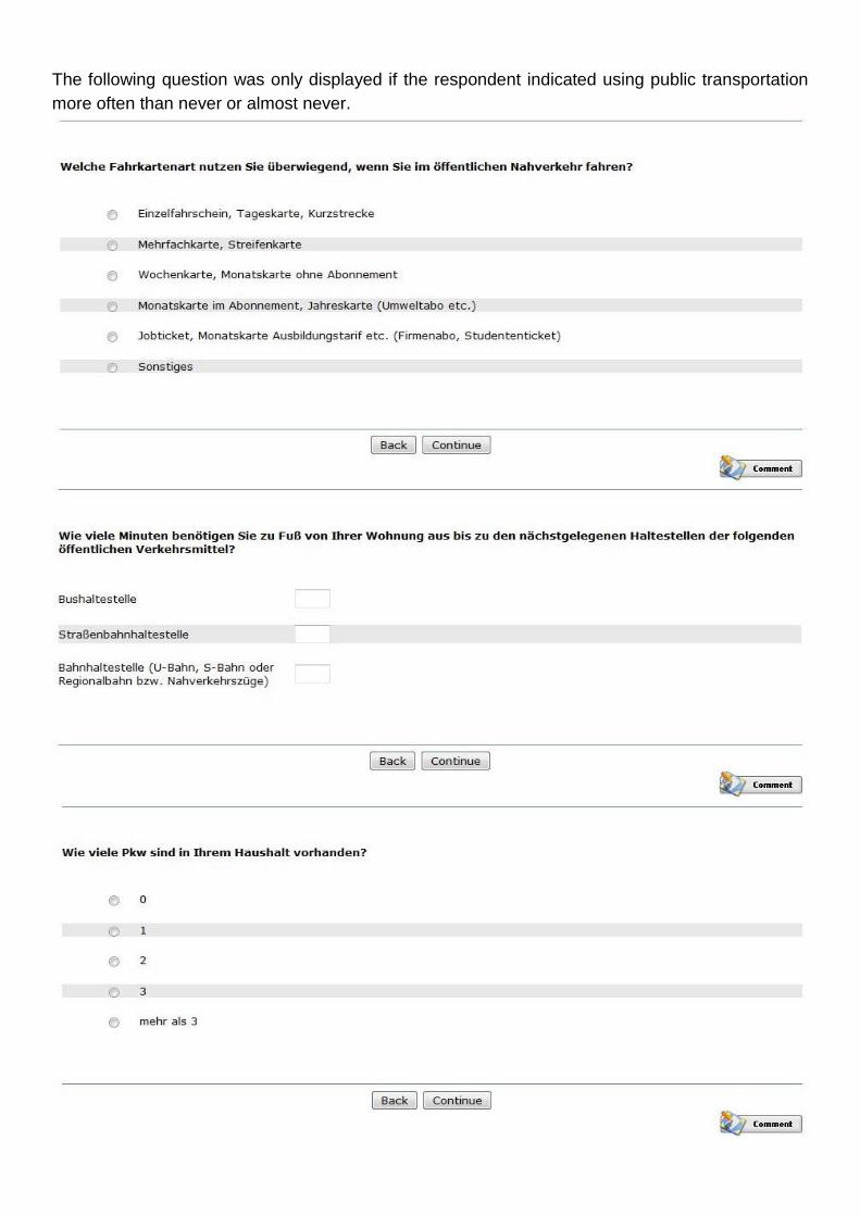
The following question was only displayed if the respondent indicated using public transportation
more often than never or almost never.
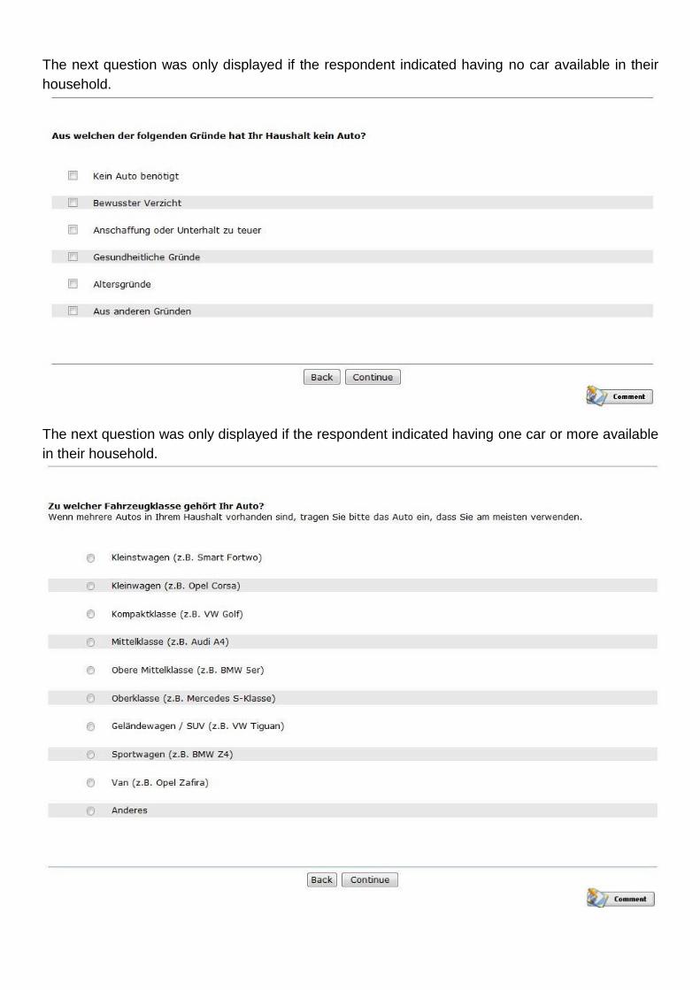
The next question was only displayed if the respondent indicated having no car available in their
household.
The next question was only displayed if the respondent indicated having one car or more available
in their household.
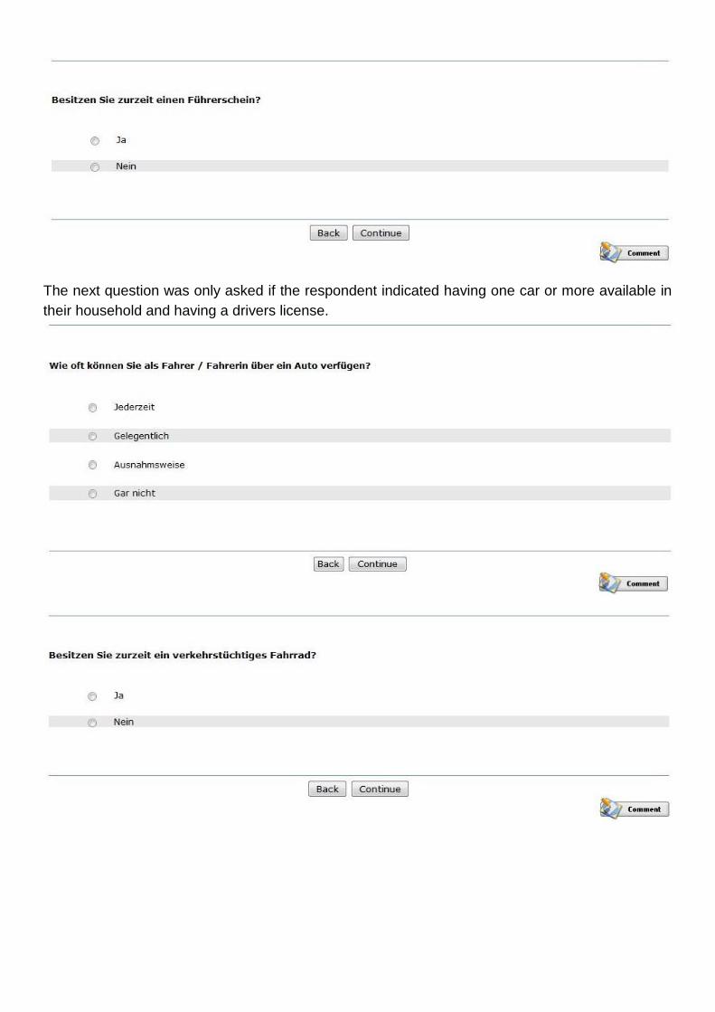
The next question was only asked if the respondent indicated having one car or more available in
their household and having a drivers license.
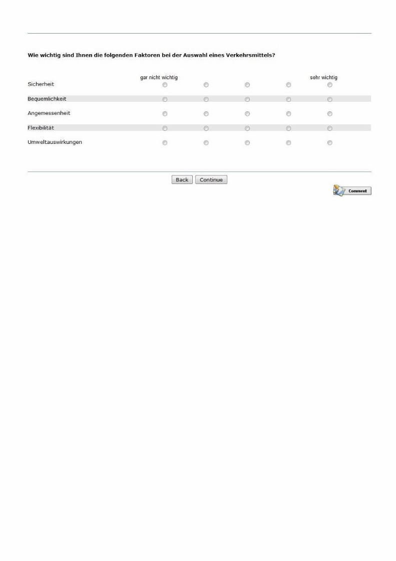
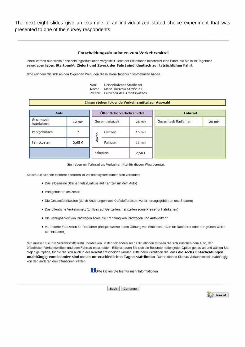
The next eight slides give an example of an individualized stated choice experiment that was
presented to one of the survey respondents.
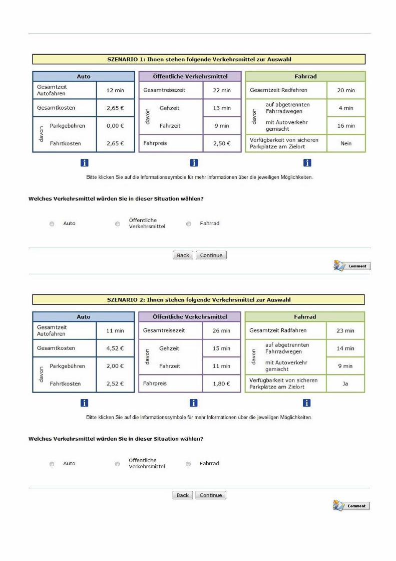
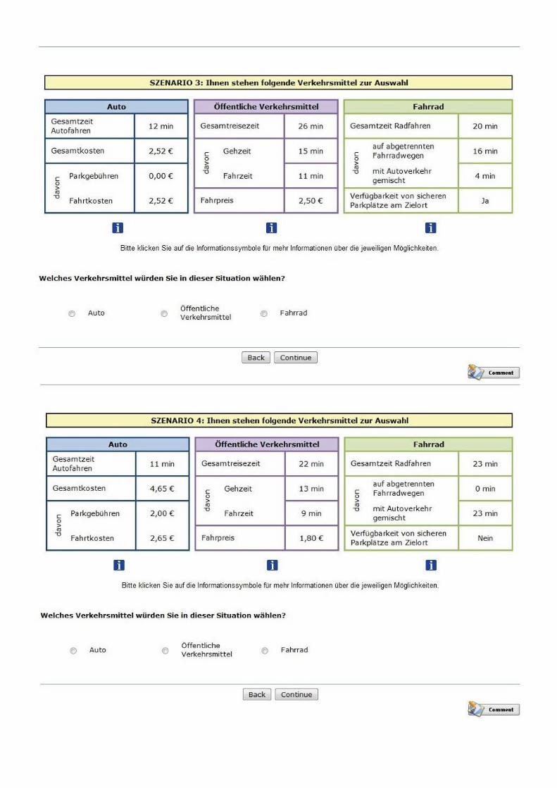

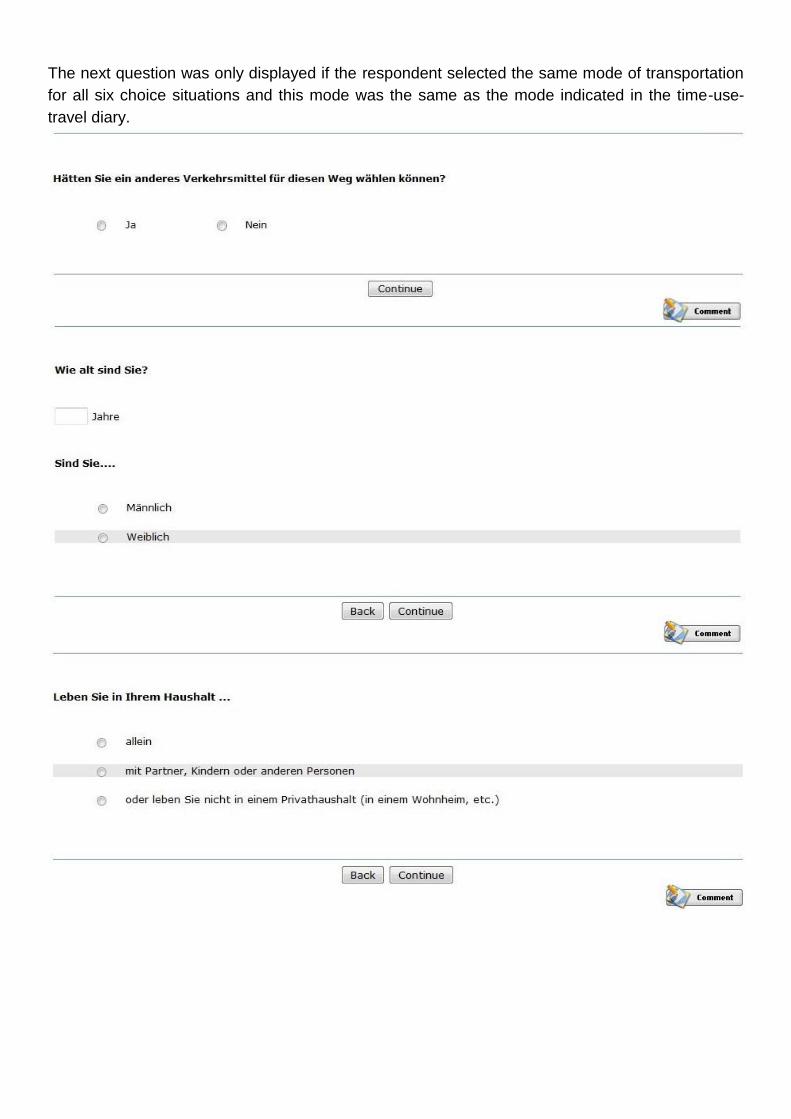
The next question was only displayed if the respondent selected the same mode of transportation
for all six choice situations and this mode was the same as the mode indicated in the time-use-
travel diary.
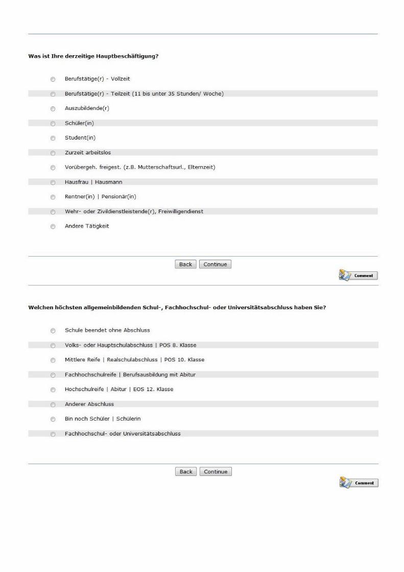


APPENDIX E - PERSONAL QUESTIONNAIRE - ENGLISH

Personal Questionnaire
1. Please indicate how often you normally use the following modes of
transportation. Please make one selection in each cross!
(almost)
Daily
1-3 days
per week
1-3 days
per month
Less than
once a
month
Never or
almost
never
Bicycle
Car
Bus, tram or train
in your region
2. How many minutes does it take to walk from your home to the nearest stations of
the following modes of public transportation? Please enter the duration of your
trip by foot! If two modes share a stop please enter the duration twice!
Bus Stop mins
Tram Station mins
Train Station
(U-Bahn, S-Bahn or
Regional Train)
mins
3. (Filter: only if question 1: Bus, tram or train in your region = more often than
never or almost never) Which type of ticket do you normally used when you use
public transportation?
1 Single ticket, day ticket, short ride ticket
2 Multi-trip ticket, stripe ticket
3 Weekly ticket, monthly ticket, monthly ticket without subscription
4 Monthly ticket with subscription, yearly ticket (Umweltabo etc.)
5 Job ticket, Semester ticket etc. (Firmenabo, Studententicket)
6 Other
4. How many cars are available in your household?
0 No car available
1 1
2 2
3 3
4 More than 3 cars

5. (Filter: only if 4 = 0) Why is there no car available in your household?
1 No car needed
2 Consciously avoid
3 Acquisition or maintenance is too expensive
4 Health reason
5 Age reason
6 Another reason
6. Do you have a driver’s license?
1 Yes
2 No
7. (Filter: only if 6 = 1 and 4 > 0) How often is a car available for you to use as a
driver or passenger?
1 Any time
2 Occasionally
3 Rarely
4 Never
8. (Filter: only if 4 > 0) Which class of vehicle does your car belong to? If there is
more than one car in your household, enter the class of the car that you use
most often.
1 Mini car (e.g. Smart Fortwo)
2 Small car (e.g. Opel Corsa)
3 Compact class (e.g. VW Golf)
4 Mid-class (e.g. Audi A4)
5 Large mid-class (e.g. BMW 5er)
6 Large class (e.g. Mercedes S-Klasse)
7 SUV (e.g. VW Tiguan)
8 Sport car (e.g. BMW Z4)
9 Van (e.g. Opel Zafira)
10 Other
9. Do you own a functioning bicycle?
1 Yes
2 No
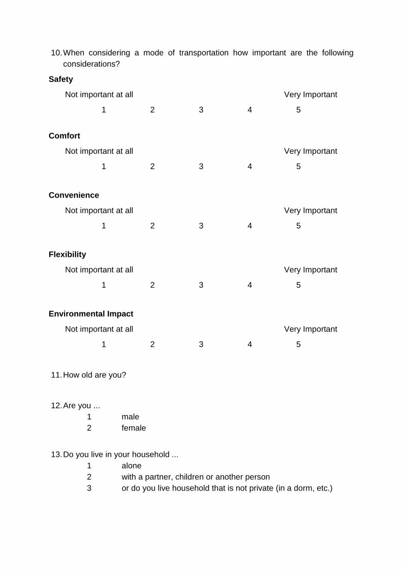
10. When considering a mode of transportation how important are the following
considerations?
Safety
Not important at all Very Important
1 2 3 4 5
Comfort
Not important at all Very Important
1 2 3 4 5
Convenience
Not important at all Very Important
1 2 3 4 5
Flexibility
Not important at all Very Important
1 2 3 4 5
Environmental Impact
Not important at all Very Important
1 2 3 4 5
11. How old are you?
12. Are you ...
1 male
2 female
13. Do you live in your household ...
1 alone
2 with a partner, children or another person
3 or do you live household that is not private (in a dorm, etc.)

14. What is your current employment situation?
1 Employed – full time
2 Employed – part time (11 to less than 35 hours/week)
3 Apprenticeship
4 Pupil (including pre-school)
5 Student (university or college)
6 Currently unemployed
7 Temporary leave (e.g. maternity leave, paternity leave)
8 Housewife | Househusband
9 Retiree
10 Military or civil service, voluntary service
11 Other
15. What level of education do you have?
1 School without graduation
2 Primary or secondary school
3 Secondary school
4 High school | Apprenticeship with graduation
5 High school with graduation
6 Other degree
7 Still a student
8 College of university degree
16. What is your household net monthly income in Euros (roughly)? Please include
all types of income, including monthly wage, salary, income from self-
employment, pension, child allowance, housing benefit or social assistance, and
other income after deducting taxes and social security contributions for all
household members.
1 Up to 500 € per month
2 500 € to less than 900 €
3 900 € to less than 1,500 €
4 1,500 € to less than 2,000 €
5 2,000 € to less than 2,600 €
6 2,600 € to less than 3,000 €
7 3,000 € to less than 3,600 €
8 3,600 € to less than 4,000 €
9 4,000 € to less than 4,600 €
10 4,600 € to less than 5,000 €
11 5,000 € to less than 5,600 €
12 5,600 € to less than 6,000 €
13 6,000 € to less than 6,600 €
14 6,600 € to 7,000 €
15 More than 7,000 € per month
97 Answer refused

APPENDIX F - STATED CHOICE EXPERIMENT – ENGLISH
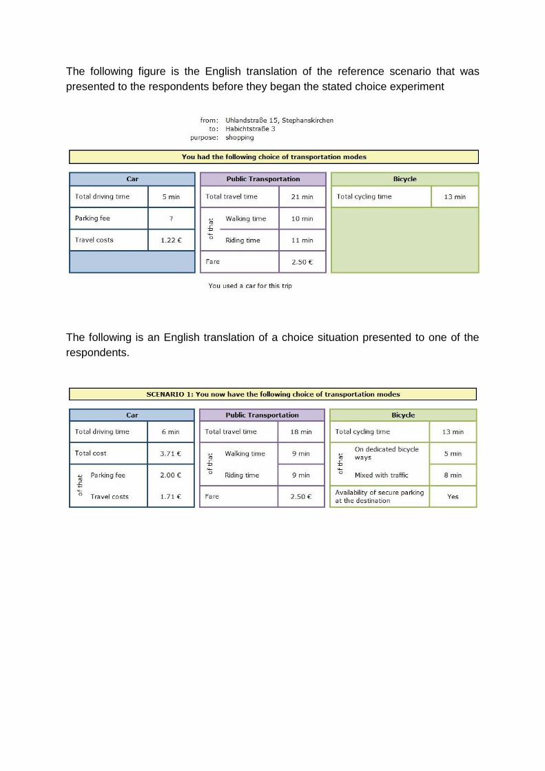
The following figure is the English translation of the reference scenario that was
presented to the respondents before they began the stated choice experiment
The following is an English translation of a choice situation presented to one of the
respondents.
APPENDIX G - STATED CHOICE EXPERIMENT - ADDITIONAL INFORMATION - GERMAN
As available to survey participants by clicking
Please see Appendix H for an English translation
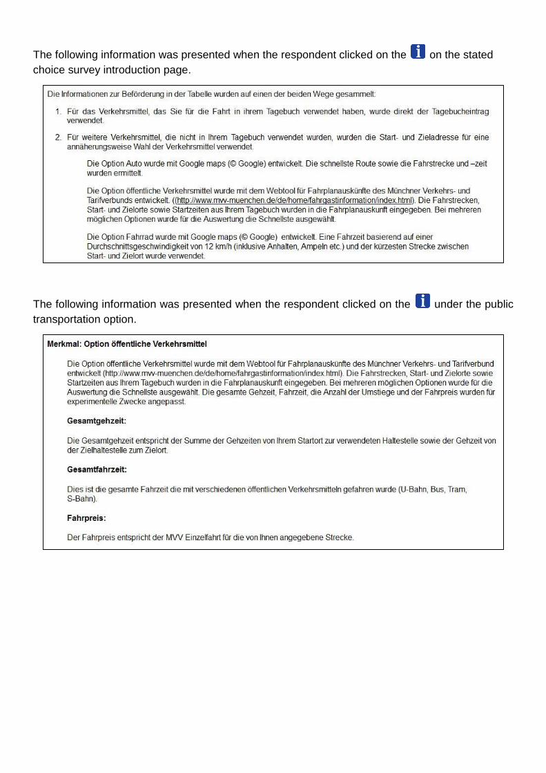
The following information was presented when the respondent clicked on the on the stated
choice survey introduction page.
The following information was presented when the respondent clicked on the under the public
transportation option.

The following information was presented when the respondent clicked on the under the car
option.
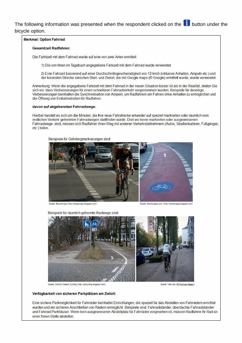
The following information was presented when the respondent clicked on the button under the
bicycle option.
APPENDIX H - STATED CHOICE EXPERIMENT - ADDITIONAL INFORMATION - ENGLISH
The following information was presented when the respondent clicked on the button on the
stated choice survey introduction page.
The transportation information presented in the table was collected in one of two ways:
1 For the mode that was used for the trip in your trip diary, the information was taken directly
from the diary.
2 For the alternative modes that were not used in your trip diary, the start and end addresses
provided in your diary were used to estimate the characteristics of the modes. This was
done using different methods for the three modes.
a. The car option was developed using Google maps (© Google). The fastest route was
selected and the distance and trip duration given by Google maps was used.
b. The public transportation option was developed with the trip planning web tool
provided by the MVV (Münchner Verkehrs- und Tarifverbund-
http://www.mvvmuenchen.de/de/home/fahrgastinformation/index.html). The start
location and end location as well as the start time indicated in your time-use-travel
diary were entered into the trip planning tool. When more than one option was given
by the web tool, the fastest option was selected.
c. The bicycle option was developed using Google maps (© Google). The travel time
was based on an average speed of 12 km/h (including stops, traffic lights, etc.) and
the shorted route between the start and end location was selected.
The following information was presented when the respondent clicked on the button under the
bicycle option.
Additional Information: Bicycle Option
Total time cycling:
The time cycling was calculated in one of two ways:
1) If a bicycle was used for the trip reported in the time-use-travel dairy, the travel time
reported in the diary was used.
2) For trips not made by a bicycle in the time-use-travel diary, a travel time based on an
average speed of 12 km/h (including stops, traffic lights, etc.) and the shortest route
between the start and end locations indicated by Google maps (© Google) was used.
Note: If the given bicycle travel is shorter than that experienced in reality, imagine that
improvements were made to increase the average speed of bicycle transportation. Examples of
such improvement include the synchronization of traffic lights for bicycles to allow cyclists to travel
without stopping, or the opening of one-way streets for bicycle traffic in both directions.
Percentage of bicycle trip on designated bicycle infrastructure:
This is the percentage of your new bicycle trip that will take place either on a marked or physically
separated bicycle way. Where no designated bicycle ways exist, cyclists must share the road or
sidewalk with other users (cars, trams, pedestrians, etc.).
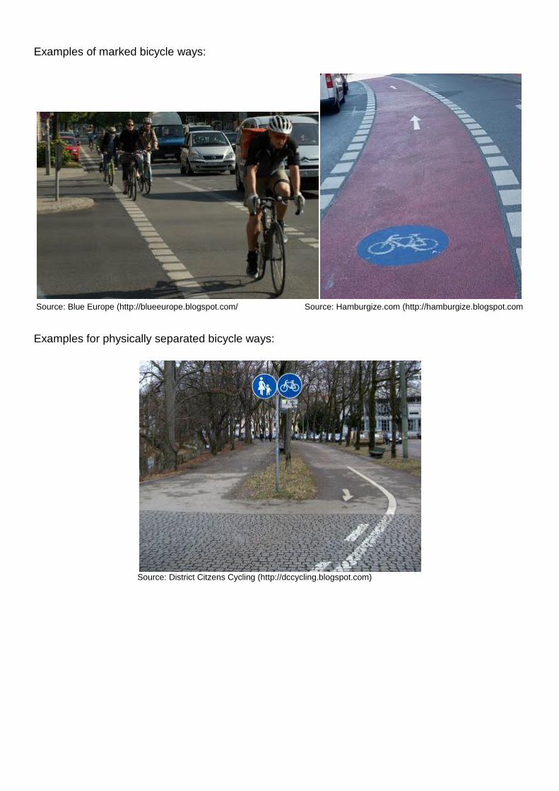
Examples of marked bicycle ways:
Source: Blue Europe (http://blueeurope.blogspot.com/ Source: Hamburgize.com (http://hamburgize.blogspot.com
Examples for physically separated bicycle ways:
Source: District Citzens Cycling (http://dccycling.blogspot.com)
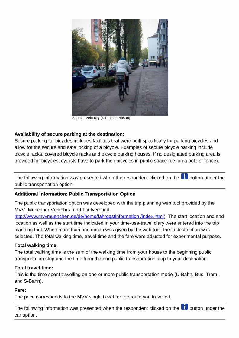
Source: Velo-city (©Thomas Hasan)
Availability of secure parking at the destination:
Secure parking for bicycles includes facilities that were built specifically for parking bicycles and
allow for the secure and safe locking of a bicycle. Examples of secure bicycle parking include
bicycle racks, covered bicycle racks and bicycle parking houses. If no designated parking area is
provided for bicycles, cyclists have to park their bicycles in public space (i.e. on a pole or fence).
The following information was presented when the respondent clicked on the button under the
public transportation option.
Additional Information: Public Transportation Option
The public transportation option was developed with the trip planning web tool provided by the
MVV (Münchner Verkehrs- und Tarifverbund
http://www.mvvmuenchen.de/de/home/fahrgastinformation /index.html). The start location and end
location as well as the start time indicated in your time-use-travel diary were entered into the trip
planning tool. When more than one option was given by the web tool, the fastest option was
selected. The total walking time, travel time and the fare were adjusted for experimental purpose.
Total walking time:
The total walking time is the sum of the walking time from your house to the beginning public
transportation stop and the time from the end public transportation stop to your destination.
Total travel time:
This is the time spent travelling on one or more public transportation mode (U-Bahn, Bus, Tram,
and S-Bahn).
Fare:
The price corresponds to the MVV single ticket for the route you travelled.
The following information was presented when the respondent clicked on the button under the
car option.
Additional Information: Car Option
Total travel time:
If a car was used in the trip recorded in your one day diary, the travel time was taken from your
diary. If the recorded trip was made using a different mode of transportation, the travel time was
estimated using you start and end addresses and Google maps (© Google). The travel time was
then adjusted for experimental purpose.
Parking fee:
The parking fee shown is the amount you would have to pay to park your vehicle for your entire
stay at your destination.
Travel cost:
The total travel cost of the trip was estimated using an average cost of 53 cents per kilometre,
which was calculated by ADAC (ADAC Autokosten 2011). This average was calculated from data
from over 1500 vehicles in Germany. For more information please see the report prepared by the
ADAC (http://www.adac.de/_mm/pdf/autokostenuebersicht_47085.pdf).

APPENDIX I – EXPERIMENTAL DESIGN
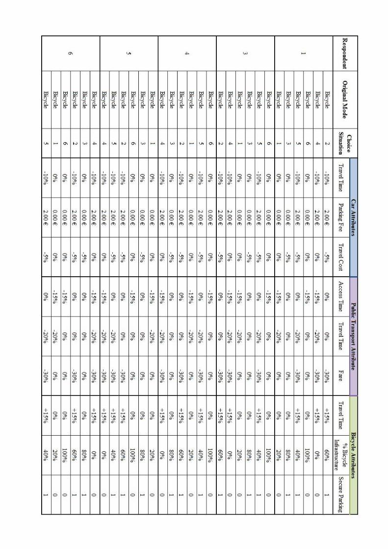
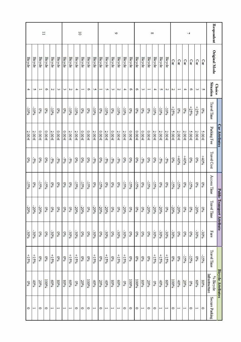


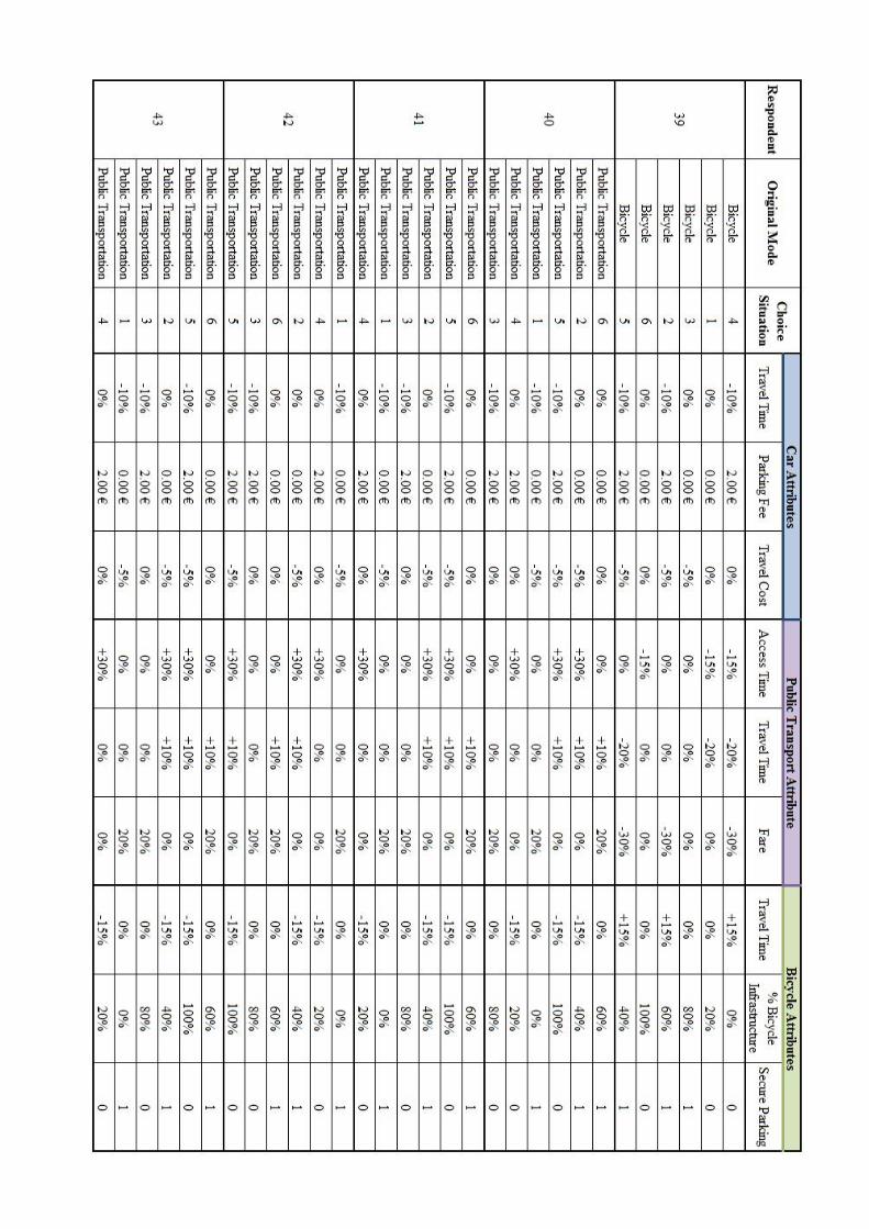
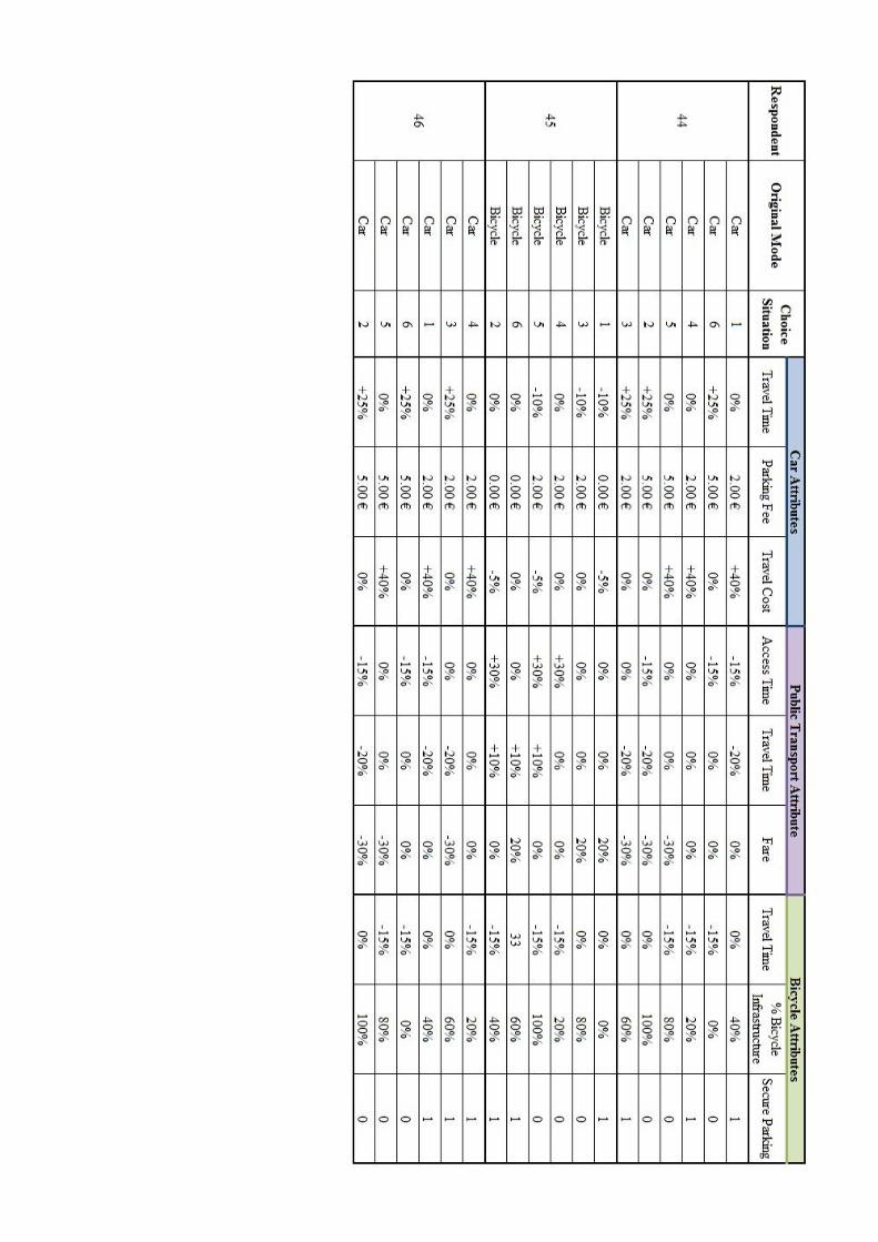

APPENDIX J – NGENE CODE USED TO PRODUCE EXPERIMENTAL DESIGN

Design
;alts(1) = car, put, bike
;alts(3) = car, put, bike
;alts(4) = car, put, bike
;alts(5) = car, put, bike
;alts(6) = car, put, bike
;alts(7) = car, put, bike
;alts(8) = car, put, bike
;alts(9) = car, put, bike
;alts(10) = car, put, bike
;alts(11) = car, put, bike
;alts(12) = car, put, bike
;alts(13) = car, put, bike
;alts(14) = car, put, bike
;alts(15) = car, put, bike
;alts(16) = car, put, bike
;alts(17) = car, put, bike
;alts(18) = car, put, bike
;alts(20) = car, put, bike
;alts(21) = car, put, bike
;alts(22) = car, put, bike
;alts(23) = car, put, bike
;alts(24) = car, put, bike
;alts(25) = car, put, bike
;alts(27) = car, put, bike
;alts(28) = car, put, bike
;alts(29) = car, put, bike
;alts(30) = car, put, bike
;alts(31) = car, put, bike
;alts(32) = car, put, bike
;alts(33) = car, put, bike
;alts(34) = car, put, bike
;alts(35) = car, put, bike
;alts(36) = car, put, bike
;alts(37) = car, put, bike
;alts(38) = car, put, bike
;alts(39) = car, put, bike
;alts(40) = car, put, bike
;alts(41) = car, put, bike
;alts(42) = car, put, bike
;alts(43) = car, put, bike
;alts(44) = car, put, bike
;alts(45) = car, put, bike
;rows = 6
;eff = choice(mnl,d)
;fisher(choice) = bike (1[0.024], 3[0.024], 4[0.024], 5[0.024], 6[0.024], 8[0.024], 9[0.024], 10[0.024], 11[0.024], 15[0.024] ,
16[0.024], 17[0.024], 18[0.024], 20[0.024], 22[0.024], 24[0.024], 27[0.024], 28[0.024], 29[0.024], 30[0.024], 34[0.024],
35[0.024], 45[0.016], 39[0.024]) + put (13[0.024], 14[0.024], 21[0.024], 23[0.024], 31[0.024], 32[0.024], 36[0.024], 38[0.024],
40[0.024], 41[0.024], 42[0.024], 43[0.024], 12[0.024]) + car (25[0.024], 33[0.024], 44[0.024], 37[0.024], 7[0.024])
;model(1):
U(car) = β0car[0.214] + β1car[-0.038]*CARTT[9,10] + β2car[-0.251]*PARK[0,2] + β3car[-0.097]*COST[2.7189,2.862] /
U(put)= β0PuT[-2.088] + β1PuT[-0.043] *ACCESS[6,7] + β2PuT[-0.032]*PuTTT[17,21] + β3PuT[-0.116]*FARE[1.8,2.5] /
U(bike) = β1bike[-0.039]* BIKETT[20,23] + β2bike[0.300] * PATHS[0,0.2,0.4,0.6,0.8,1] + β3bike [1.459] * BPARK[0,1]
;model(3):
U(car) = β0car[0.214] + β1car[-0.038]*CARTT[14,15] + β2car[-0.251]*PARK[0,2] + β3car[-0.097]*COST[3.8266,4.028] /
U(put)= β0put[-2.088] + β1PuT[-0.043] *ACCESS[17,20] + β2PuT[-0.032]*PuTTT[14,17] + β3PuT[-0.116]*FARE[1.8,2.5] /
U(bike) = β1bike[-0.039]* BIKETT[30,35] + β2bike[0.300] * PATHS[0,0.2,0.4,0.6,0.8,1] + β3bike[1.459] * BPARK[0,1]
;model(4):
U(car) = β0car[0.214] + β1car[-0.038]*CARTT[5,6] + β2car[-0.251]*PARK[0,2] + β3car[-0.097]*COST[1.4098,1.484] /
U(put)= β0put[-2.088] + β1PuT[-0.043] *ACCESS[11,13] + β2PuT[-0.032]*PuTTT[9,11] + β3PuT[-0.116]*FARE[1.8,2.5] /
U(bike) = β1bike[-0.039]* BIKETT[13,15] + β2bike[0.300] * PATHS[0,0.2,0.4,0.6,0.8,1] + β3bike[1.459] * BPARK[0,1]
;model(5):

U(car) = β0car[0.214] + β1car[-0.038]*CARTT[5,6] + β2car[-0.251]*PARK[0,2] + β3car[-0.097]*COST[1.4098,1.484] /
U(put)= β0put[-2.088] + β1PuT[-0.043] *ACCESS[11,13] + β2PuT[-0.032]*PuTTT[9,11] + β3PuT[-0.116]*FARE[1.8,2.5] /
U(bike) = β1bike[-0.039]* BIKETT[25,29] + β2bike[0.300] * PATHS[0,0.2,0.4,0.6,0.8,1] + β3bike[1.459] * BPARK[0,1]
;model(6):
U(car) = β0car[0.214] + β1car[-0.038]*CARTT[5,6] + β2car[-0.251]*PARK[0,2] + β3car[-0.097]*COST[1.9133,2.014] /
U(put)= β0put[-2.088] + β1PuT[-0.043] *ACCESS[11,13] + β2PuT[-0.032]*PuTTT[9,11] + β3PuT[-0.116]*FARE[1.8,2.5] /
U(bike) = β1bike[-0.039]* BIKETT[15,17] + β2bike[0.300] * PATHS[0,0.2,0.4,0.6,0.8,1] + β3bike[1.459] * BPARK[0,1]
;model(7):
U(car) = β0car[0.214] + β1car[-0.038]*CARTT[25,31] + β2car[-0.251]*PARK[2,5] + β3car[-0.097]*COST[10.971,15.3594] /
U(put)= β0put[-2.088] + β1PuT[-0.043] *ACCESS[13,15] + β2PuT[-0.032]*PuTTT[21,26] + β3PuT[-0.116]*FARE[3.5,5] /
U(bike) = β1bike[-0.039]* BIKETT[85,100] + β2bike[0.300] * PATHS[0,0.2,0.4,0.6,0.8,1] + β3bike[1.459] * BPARK[0,1]
;model(8):
U(car) = β0car[0.214] + β1car[-0.038]*CARTT[7,8] + β2car[-0.251]*PARK[0,2] + β3car[-0.097]*COST[1.7119,1.802] /
U(put)= β0put[-2.088] + β1PuT[-0.043] *ACCESS[7,8] + βpCARTT[-0.032]*PuTTT[11,14] + β3PuT[-0.116]*FARE[1.8,2.5] /
U(bike) = β1bike[-0.039]* BIKETT[20,23] + β2bike[0.300] * PATHS[0,0.2,0.4,0.6,0.8,1] + β3bike[1.459] * BPARK[0,1]
;model(9):
U(car) = β0car[0.214] + β1car[-0.038]*CARTT[10,11] + β2car[-0.251]*PARK[0,2] + β3car[-0.097]*COST[2.97065,3.127] /
U(put)= β0put[-2.088] + β1PuT[-0.043] *ACCESS[4,5] + βPuTTT[-0.032]*PuTTT[6,7] + β3PuT[-0.116]*FARE[1.8,2.5] /
U(bike) = β1bike[-0.039]* BIKETT[30,35] + β2bike[0.300] * PATHS[0,0.2,0.4,0.6,0.8,1] + β3bike[1.459] * BPARK[0,1]
;model(10):
U(car) = β0car[0.214] + β1car[-0.038]*CARTT[15,17] + β2car[-0.251]*PARK[0,2] + β3car[-0.097]*COST[5.08535,5.353] /
U(put)= β0put[-2.088] + β1PuT[-0.043] *ACCESS[13,15] + βPuTTT[-0.032]*PuTTT[21,26] + β3PuT[-0.116]*FARE[1.8,2.5] /
U(bike) = β1bike[-0.039]* BIKETT[25,29] + β2bike[0.300] * PATHS[0,0.2,0.4,0.6,0.8,1] + β3bike[1.459] * BPARK[0,1]
;model(11):
U(car) = β0car[0.214] + β1car[-0.038]*CARTT[5,6] + β2car[-0.251]*PARK[0,2] + β3car[-0.097]*COST[1.007,1.06] /
U(put)= β0put[-2.088] + β1PuT[-0.043] *ACCESS[7,8] + β2PuT[-0.032]*PuTTT[7,9] + β3PuT[-0.116]*FARE[1.8,2.5] /
U(bike) = β1bike[-0.039]* BIKETT[10,12] + β2bike[0.300] * PATHS[0,0.2,0.4,0.6,0.8,1] + β3bike[1.459] * BPARK[0,1]
;model(12):
U(car) = β0car[0.214] + β1car[-0.038]*CARTT[20,22] + β2car[-0.251]*PARK[0,2] + β3car[-0.097]*COST[3.27275,3.445] /
U(put)= β0put[-2.088] + β1PuT[-0.043] *ACCESS[24,31] + β2PuT[-0.032]*PuTTT[9,10] + β3PuT[-0.116]*FARE[2.5,3] /
U(bike) = β1bike[-0.039]* BIKETT[33,39] + β2bike[0.300] * PATHS[0,0.2,0.4,0.6,0.8,1] + β3bike[1.459] * BPARK[0,1]
;model(13):
U(car) = β0car[0.214] + β1car[-0.038]*CARTT[17,19] + β2car[-0.251]*PARK[0,2] + β3car[-0.097]*COST[6.2434,6.572] /
U(put)= β0put[-2.088] + β1PuT[-0.043] *ACCESS[13,17] + β2PuT[-0.032]*PuTTT[23,25] + β3PuT[-0.116]*FARE[2.5,3] /
U(bike) = β1bike[-0.039]* BIKETT[51,60] + β2bike[0.300] * PATHS[0,0.2,0.4,0.6,0.8,1] + β3bike[1.459] * BPARK[0,1]
;model(14):
U(car) = β0car[0.214] + β1car[-0.038]*CARTT[17,19] + β2car[-0.251]*PARK[0,2] + β3car[-0.097]*COST[4.58185,4.823] /
U(put)= β0put[-2.088] + β1PuT[-0.043] *ACCESS[6,8] + β2PuT[-0.032]*PuTTT[15,17] + β3PuT[-0.116]*FARE[2.5,3] /
U(bike) = β1bike[-0.039]* BIKETT[40,47] + β2bike[0.300] * PATHS[0,0.2,0.4,0.6,0.8,1] + β3bike[1.459] * BPARK[0,1]
;model(15):
U(car) = β0car[0.214] + β1car[-0.038]*CARTT[3,4] + β2car[-0.251]*PARK[0,2] + β3car[-0.097]*COST[0.55385,0.583] /
U(put)= β0put[-2.088] + β1PuT[-0.043] *ACCESS[7,8] + β2PuT[-0.032]*PuTTT[1,2] + β3PuT[-0.116]*FARE[0.8,1.2] /
U(bike) = β1bike[-0.039]* BIKETT[5,6] + β2bike[0.300] * PATHS[0,0.2,0.4,0.6,0.8,1] + β3bike[1.459] * BPARK[0,1]
;model(16):
U(car) = β0car[0.214] + β1car[-0.038]*CARTT[14,15] + β2car[-0.251]*PARK[0,2] + β3car[-0.097]*COST[3.3231,3.498] /
U(put)= β0put[-2.088] + β1PuT[-0.043] *ACCESS[9,11] + β2PuT[-0.032]*PuTTT[8,10] + β3PuT[-0.116]*FARE[1.8,2.5] /
U(bike) = β1bike[-0.039]* BIKETT[20,23] + β2bike[0.300] * PATHS[0,0.2,0.4,0.6,0.8,1] + β3bike[1.459] * BPARK[0,1]
;model(17):
U(car) = β0car[0.214] + β1car[-0.038]*CARTT[11,12] + β2car[-0.251]*PARK[0,2] + β3car[-0.097]*COST[2.5175,2.65] /
U(put)= β0put[-2.088] + β1PuT[-0.043] *ACCESS[13,15] + β2PuT[-0.032]*PuTTT[9,11] + β3PuT[-0.116]*FARE[1.8,2.5] /
U(bike) = β1bike[-0.039]* BIKETT[20,23] + β2bike[0.300] * PATHS[0,0.2,0.4,0.6,0.8,1] + β3bike[1.459] * BPARK[0,1]
;model(18):
U(car) = β0car[0.214] + β1car[-0.038]*CARTT[4,5] + β2car[-0.251]*PARK[0,2] + β3car[-0.097]*COST[0.8056,0.848] /
U(put)= β0put[-2.088] + β1PuT[-0.043] *ACCESS[11,13] + β2PuT[-0.032]*PuTTT[1,2] + β3PuT[-0.116]*FARE[0.8,1.2] /
U(bike) = β1bike[-0.039]* BIKETT[5,6] + β2bike[0.300] * PATHS[0,0.2,0.4,0.6,0.8,1] + β3bike[1.459] * BPARK[0,1]
;model(20):
U(car) = β0car[0.214] + β1car[-0.038]*CARTT[8,9] + β2car[-0.251]*PARK[0,2] + β3car[-0.097]*COST[2.26575,2.385] /
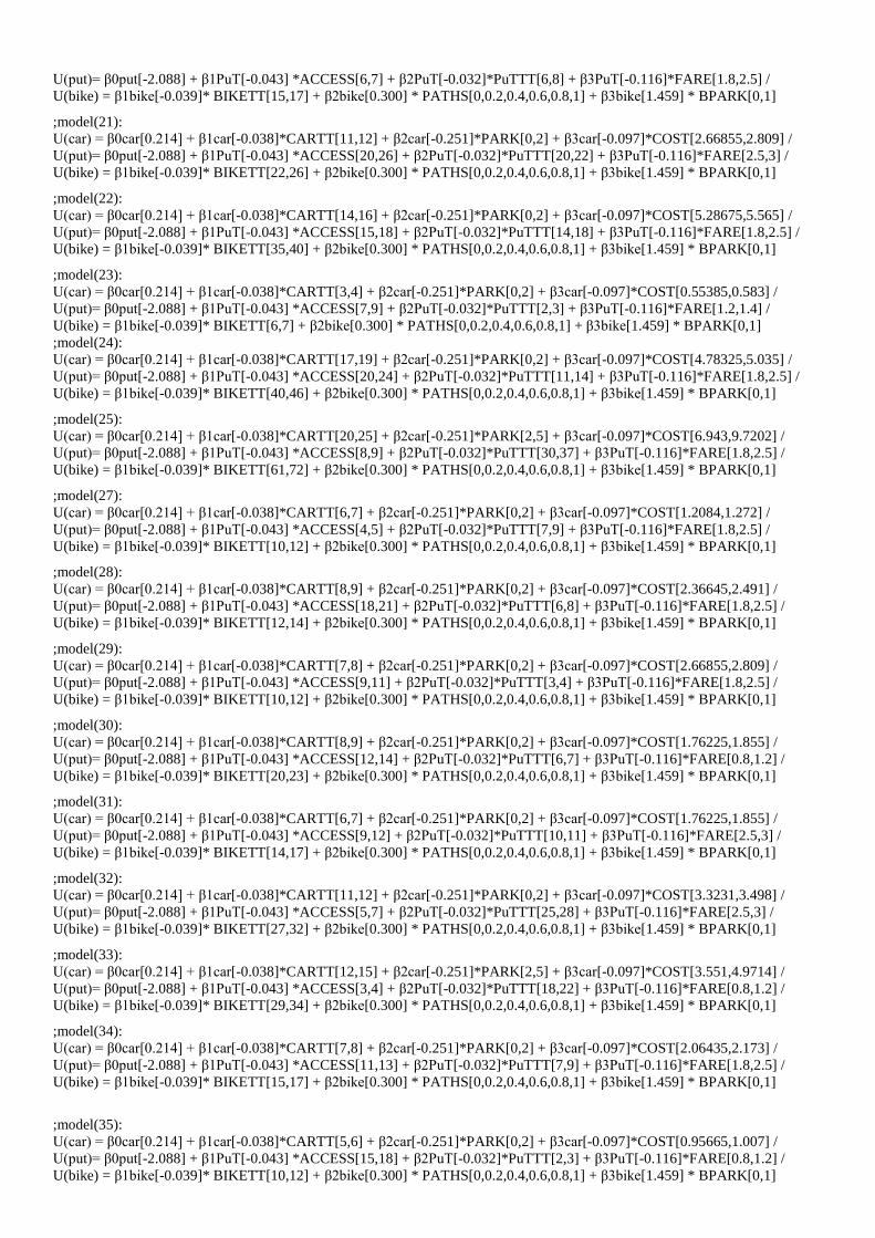
U(put)= β0put[-2.088] + β1PuT[-0.043] *ACCESS[6,7] + β2PuT[-0.032]*PuTTT[6,8] + β3PuT[-0.116]*FARE[1.8,2.5] /
U(bike) = β1bike[-0.039]* BIKETT[15,17] + β2bike[0.300] * PATHS[0,0.2,0.4,0.6,0.8,1] + β3bike[1.459] * BPARK[0,1]
;model(21):
U(car) = β0car[0.214] + β1car[-0.038]*CARTT[11,12] + β2car[-0.251]*PARK[0,2] + β3car[-0.097]*COST[2.66855,2.809] /
U(put)= β0put[-2.088] + β1PuT[-0.043] *ACCESS[20,26] + β2PuT[-0.032]*PuTTT[20,22] + β3PuT[-0.116]*FARE[2.5,3] /
U(bike) = β1bike[-0.039]* BIKETT[22,26] + β2bike[0.300] * PATHS[0,0.2,0.4,0.6,0.8,1] + β3bike[1.459] * BPARK[0,1]
;model(22):
U(car) = β0car[0.214] + β1car[-0.038]*CARTT[14,16] + β2car[-0.251]*PARK[0,2] + β3car[-0.097]*COST[5.28675,5.565] /
U(put)= β0put[-2.088] + β1PuT[-0.043] *ACCESS[15,18] + β2PuT[-0.032]*PuTTT[14,18] + β3PuT[-0.116]*FARE[1.8,2.5] /
U(bike) = β1bike[-0.039]* BIKETT[35,40] + β2bike[0.300] * PATHS[0,0.2,0.4,0.6,0.8,1] + β3bike[1.459] * BPARK[0,1]
;model(23):
U(car) = β0car[0.214] + β1car[-0.038]*CARTT[3,4] + β2car[-0.251]*PARK[0,2] + β3car[-0.097]*COST[0.55385,0.583] /
U(put)= β0put[-2.088] + β1PuT[-0.043] *ACCESS[7,9] + β2PuT[-0.032]*PuTTT[2,3] + β3PuT[-0.116]*FARE[1.2,1.4] /
U(bike) = β1bike[-0.039]* BIKETT[6,7] + β2bike[0.300] * PATHS[0,0.2,0.4,0.6,0.8,1] + β3bike[1.459] * BPARK[0,1]
;model(24):
U(car) = β0car[0.214] + β1car[-0.038]*CARTT[17,19] + β2car[-0.251]*PARK[0,2] + β3car[-0.097]*COST[4.78325,5.035] /
U(put)= β0put[-2.088] + β1PuT[-0.043] *ACCESS[20,24] + β2PuT[-0.032]*PuTTT[11,14] + β3PuT[-0.116]*FARE[1.8,2.5] /
U(bike) = β1bike[-0.039]* BIKETT[40,46] + β2bike[0.300] * PATHS[0,0.2,0.4,0.6,0.8,1] + β3bike[1.459] * BPARK[0,1]
;model(25):
U(car) = β0car[0.214] + β1car[-0.038]*CARTT[20,25] + β2car[-0.251]*PARK[2,5] + β3car[-0.097]*COST[6.943,9.7202] /
U(put)= β0put[-2.088] + β1PuT[-0.043] *ACCESS[8,9] + β2PuT[-0.032]*PuTTT[30,37] + β3PuT[-0.116]*FARE[1.8,2.5] /
U(bike) = β1bike[-0.039]* BIKETT[61,72] + β2bike[0.300] * PATHS[0,0.2,0.4,0.6,0.8,1] + β3bike[1.459] * BPARK[0,1]
;model(27):
U(car) = β0car[0.214] + β1car[-0.038]*CARTT[6,7] + β2car[-0.251]*PARK[0,2] + β3car[-0.097]*COST[1.2084,1.272] /
U(put)= β0put[-2.088] + β1PuT[-0.043] *ACCESS[4,5] + β2PuT[-0.032]*PuTTT[7,9] + β3PuT[-0.116]*FARE[1.8,2.5] /
U(bike) = β1bike[-0.039]* BIKETT[10,12] + β2bike[0.300] * PATHS[0,0.2,0.4,0.6,0.8,1] + β3bike[1.459] * BPARK[0,1]
;model(28):
U(car) = β0car[0.214] + β1car[-0.038]*CARTT[8,9] + β2car[-0.251]*PARK[0,2] + β3car[-0.097]*COST[2.36645,2.491] /
U(put)= β0put[-2.088] + β1PuT[-0.043] *ACCESS[18,21] + β2PuT[-0.032]*PuTTT[6,8] + β3PuT[-0.116]*FARE[1.8,2.5] /
U(bike) = β1bike[-0.039]* BIKETT[12,14] + β2bike[0.300] * PATHS[0,0.2,0.4,0.6,0.8,1] + β3bike[1.459] * BPARK[0,1]
;model(29):
U(car) = β0car[0.214] + β1car[-0.038]*CARTT[7,8] + β2car[-0.251]*PARK[0,2] + β3car[-0.097]*COST[2.66855,2.809] /
U(put)= β0put[-2.088] + β1PuT[-0.043] *ACCESS[9,11] + β2PuT[-0.032]*PuTTT[3,4] + β3PuT[-0.116]*FARE[1.8,2.5] /
U(bike) = β1bike[-0.039]* BIKETT[10,12] + β2bike[0.300] * PATHS[0,0.2,0.4,0.6,0.8,1] + β3bike[1.459] * BPARK[0,1]
;model(30):
U(car) = β0car[0.214] + β1car[-0.038]*CARTT[8,9] + β2car[-0.251]*PARK[0,2] + β3car[-0.097]*COST[1.76225,1.855] /
U(put)= β0put[-2.088] + β1PuT[-0.043] *ACCESS[12,14] + β2PuT[-0.032]*PuTTT[6,7] + β3PuT[-0.116]*FARE[0.8,1.2] /
U(bike) = β1bike[-0.039]* BIKETT[20,23] + β2bike[0.300] * PATHS[0,0.2,0.4,0.6,0.8,1] + β3bike[1.459] * BPARK[0,1]
;model(31):
U(car) = β0car[0.214] + β1car[-0.038]*CARTT[6,7] + β2car[-0.251]*PARK[0,2] + β3car[-0.097]*COST[1.76225,1.855] /
U(put)= β0put[-2.088] + β1PuT[-0.043] *ACCESS[9,12] + β2PuT[-0.032]*PuTTT[10,11] + β3PuT[-0.116]*FARE[2.5,3] /
U(bike) = β1bike[-0.039]* BIKETT[14,17] + β2bike[0.300] * PATHS[0,0.2,0.4,0.6,0.8,1] + β3bike[1.459] * BPARK[0,1]
;model(32):
U(car) = β0car[0.214] + β1car[-0.038]*CARTT[11,12] + β2car[-0.251]*PARK[0,2] + β3car[-0.097]*COST[3.3231,3.498] /
U(put)= β0put[-2.088] + β1PuT[-0.043] *ACCESS[5,7] + β2PuT[-0.032]*PuTTT[25,28] + β3PuT[-0.116]*FARE[2.5,3] /
U(bike) = β1bike[-0.039]* BIKETT[27,32] + β2bike[0.300] * PATHS[0,0.2,0.4,0.6,0.8,1] + β3bike[1.459] * BPARK[0,1]
;model(33):
U(car) = β0car[0.214] + β1car[-0.038]*CARTT[12,15] + β2car[-0.251]*PARK[2,5] + β3car[-0.097]*COST[3.551,4.9714] /
U(put)= β0put[-2.088] + β1PuT[-0.043] *ACCESS[3,4] + β2PuT[-0.032]*PuTTT[18,22] + β3PuT[-0.116]*FARE[0.8,1.2] /
U(bike) = β1bike[-0.039]* BIKETT[29,34] + β2bike[0.300] * PATHS[0,0.2,0.4,0.6,0.8,1] + β3bike[1.459] * BPARK[0,1]
;model(34):
U(car) = β0car[0.214] + β1car[-0.038]*CARTT[7,8] + β2car[-0.251]*PARK[0,2] + β3car[-0.097]*COST[2.06435,2.173] /
U(put)= β0put[-2.088] + β1PuT[-0.043] *ACCESS[11,13] + β2PuT[-0.032]*PuTTT[7,9] + β3PuT[-0.116]*FARE[1.8,2.5] /
U(bike) = β1bike[-0.039]* BIKETT[15,17] + β2bike[0.300] * PATHS[0,0.2,0.4,0.6,0.8,1] + β3bike[1.459] * BPARK[0,1]
;model(35):
U(car) = β0car[0.214] + β1car[-0.038]*CARTT[5,6] + β2car[-0.251]*PARK[0,2] + β3car[-0.097]*COST[0.95665,1.007] /
U(put)= β0put[-2.088] + β1PuT[-0.043] *ACCESS[15,18] + β2PuT[-0.032]*PuTTT[2,3] + β3PuT[-0.116]*FARE[0.8,1.2] /
U(bike) = β1bike[-0.039]* BIKETT[10,12] + β2bike[0.300] * PATHS[0,0.2,0.4,0.6,0.8,1] + β3bike[1.459] * BPARK[0,1]
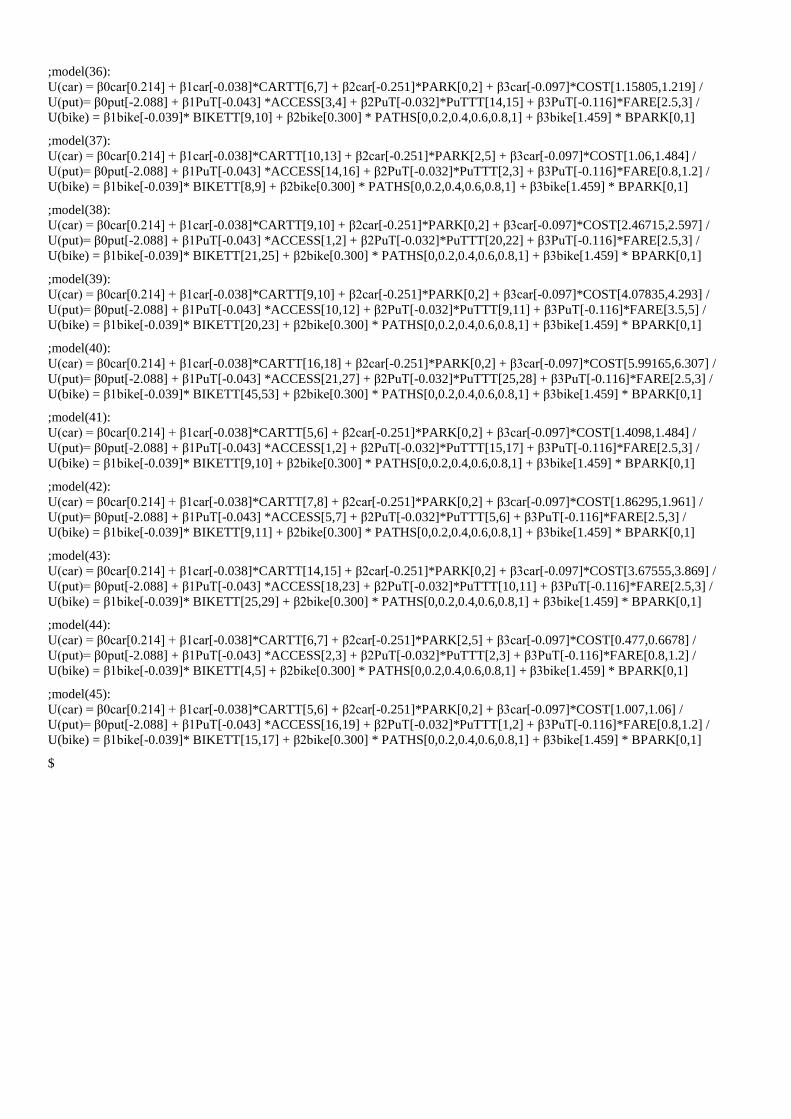
;model(36):
U(car) = β0car[0.214] + β1car[-0.038]*CARTT[6,7] + β2car[-0.251]*PARK[0,2] + β3car[-0.097]*COST[1.15805,1.219] /
U(put)= β0put[-2.088] + β1PuT[-0.043] *ACCESS[3,4] + β2PuT[-0.032]*PuTTT[14,15] + β3PuT[-0.116]*FARE[2.5,3] /
U(bike) = β1bike[-0.039]* BIKETT[9,10] + β2bike[0.300] * PATHS[0,0.2,0.4,0.6,0.8,1] + β3bike[1.459] * BPARK[0,1]
;model(37):
U(car) = β0car[0.214] + β1car[-0.038]*CARTT[10,13] + β2car[-0.251]*PARK[2,5] + β3car[-0.097]*COST[1.06,1.484] /
U(put)= β0put[-2.088] + β1PuT[-0.043] *ACCESS[14,16] + β2PuT[-0.032]*PuTTT[2,3] + β3PuT[-0.116]*FARE[0.8,1.2] /
U(bike) = β1bike[-0.039]* BIKETT[8,9] + β2bike[0.300] * PATHS[0,0.2,0.4,0.6,0.8,1] + β3bike[1.459] * BPARK[0,1]
;model(38):
U(car) = β0car[0.214] + β1car[-0.038]*CARTT[9,10] + β2car[-0.251]*PARK[0,2] + β3car[-0.097]*COST[2.46715,2.597] /
U(put)= β0put[-2.088] + β1PuT[-0.043] *ACCESS[1,2] + β2PuT[-0.032]*PuTTT[20,22] + β3PuT[-0.116]*FARE[2.5,3] /
U(bike) = β1bike[-0.039]* BIKETT[21,25] + β2bike[0.300] * PATHS[0,0.2,0.4,0.6,0.8,1] + β3bike[1.459] * BPARK[0,1]
;model(39):
U(car) = β0car[0.214] + β1car[-0.038]*CARTT[9,10] + β2car[-0.251]*PARK[0,2] + β3car[-0.097]*COST[4.07835,4.293] /
U(put)= β0put[-2.088] + β1PuT[-0.043] *ACCESS[10,12] + β2PuT[-0.032]*PuTTT[9,11] + β3PuT[-0.116]*FARE[3.5,5] /
U(bike) = β1bike[-0.039]* BIKETT[20,23] + β2bike[0.300] * PATHS[0,0.2,0.4,0.6,0.8,1] + β3bike[1.459] * BPARK[0,1]
;model(40):
U(car) = β0car[0.214] + β1car[-0.038]*CARTT[16,18] + β2car[-0.251]*PARK[0,2] + β3car[-0.097]*COST[5.99165,6.307] /
U(put)= β0put[-2.088] + β1PuT[-0.043] *ACCESS[21,27] + β2PuT[-0.032]*PuTTT[25,28] + β3PuT[-0.116]*FARE[2.5,3] /
U(bike) = β1bike[-0.039]* BIKETT[45,53] + β2bike[0.300] * PATHS[0,0.2,0.4,0.6,0.8,1] + β3bike[1.459] * BPARK[0,1]
;model(41):
U(car) = β0car[0.214] + β1car[-0.038]*CARTT[5,6] + β2car[-0.251]*PARK[0,2] + β3car[-0.097]*COST[1.4098,1.484] /
U(put)= β0put[-2.088] + β1PuT[-0.043] *ACCESS[1,2] + β2PuT[-0.032]*PuTTT[15,17] + β3PuT[-0.116]*FARE[2.5,3] /
U(bike) = β1bike[-0.039]* BIKETT[9,10] + β2bike[0.300] * PATHS[0,0.2,0.4,0.6,0.8,1] + β3bike[1.459] * BPARK[0,1]
;model(42):
U(car) = β0car[0.214] + β1car[-0.038]*CARTT[7,8] + β2car[-0.251]*PARK[0,2] + β3car[-0.097]*COST[1.86295,1.961] /
U(put)= β0put[-2.088] + β1PuT[-0.043] *ACCESS[5,7] + β2PuT[-0.032]*PuTTT[5,6] + β3PuT[-0.116]*FARE[2.5,3] /
U(bike) = β1bike[-0.039]* BIKETT[9,11] + β2bike[0.300] * PATHS[0,0.2,0.4,0.6,0.8,1] + β3bike[1.459] * BPARK[0,1]
;model(43):
U(car) = β0car[0.214] + β1car[-0.038]*CARTT[14,15] + β2car[-0.251]*PARK[0,2] + β3car[-0.097]*COST[3.67555,3.869] /
U(put)= β0put[-2.088] + β1PuT[-0.043] *ACCESS[18,23] + β2PuT[-0.032]*PuTTT[10,11] + β3PuT[-0.116]*FARE[2.5,3] /
U(bike) = β1bike[-0.039]* BIKETT[25,29] + β2bike[0.300] * PATHS[0,0.2,0.4,0.6,0.8,1] + β3bike[1.459] * BPARK[0,1]
;model(44):
U(car) = β0car[0.214] + β1car[-0.038]*CARTT[6,7] + β2car[-0.251]*PARK[2,5] + β3car[-0.097]*COST[0.477,0.6678] /
U(put)= β0put[-2.088] + β1PuT[-0.043] *ACCESS[2,3] + β2PuT[-0.032]*PuTTT[2,3] + β3PuT[-0.116]*FARE[0.8,1.2] /
U(bike) = β1bike[-0.039]* BIKETT[4,5] + β2bike[0.300] * PATHS[0,0.2,0.4,0.6,0.8,1] + β3bike[1.459] * BPARK[0,1]
;model(45):
U(car) = β0car[0.214] + β1car[-0.038]*CARTT[5,6] + β2car[-0.251]*PARK[0,2] + β3car[-0.097]*COST[1.007,1.06] /
U(put)= β0put[-2.088] + β1PuT[-0.043] *ACCESS[16,19] + β2PuT[-0.032]*PuTTT[1,2] + β3PuT[-0.116]*FARE[0.8,1.2] /
U(bike) = β1bike[-0.039]* BIKETT[15,17] + β2bike[0.300] * PATHS[0,0.2,0.4,0.6,0.8,1] + β3bike[1.459] * BPARK[0,1]
$

STATEMENT A methodology for the quantitative estimation of the independent influence of various mode and trip attributes is proposed, tested and qualitatively evaluated. A stated choice experiment based on reference scenarios is used as a tool to collect choice information.
München, November 04, 2011 _____________________________________ Signature ___________________________________________ Heather A. Twaddle