Using stated-preference data to estimate a structural model ofretirement and savings∗

Luc Bissonnette†

September 11, 2011

VERSION PRÉLIMINAIRE ET INCOMPLÈTE POUR ÉVALUATION PAR LE COMITÉ SCIEN-TIFIQUE DES JOURNÉES DU CIRPÉE 2011. UNE VERSIONMISE À JOUR SERADISPONIBLEPOUR LA PRÉSENTATION.

Abstract

This paper proposes to estimate a life-cycle model of retirement and savings based on stated-preference data, obtained by asking survey respondents to evaluate hypothetical retirement sce-narios. These models are usually estimated using revealed preferences inferred from actualretirement plans, an approach requiring a substantial amount of information concerning the de-tails of these plans, the availability of alternative plans, and respondents’ expectations. Usinga stated preference approach simplifies the problem by providing the relevant information onavailable plans to the respondents. I show that answers to simple questions are sufficient toestimate the model. The econometric specification I propose, a rank-ordered logit model, is easyto estimate and is, to some extent, robust to heterogeneity in answering behavior. The estimatedparameters are sensible and comparable to findings from the past literature, despite the modestsize of the sample used and the limited information available. For instance, I find a yearly dis-count parameter between 0.95 and 0.97. The implications of these results are illustrated withsimulations, with a particular emphasis on simulating the effect of a recent reform of the Dutchsocial security system.

Keywords: Aging and retirement; structural econometrics; stated-preferences; life-cycle model.JEL Codes: C81, D91, H55, J26.

∗I want to thank Rob Alessie, Marike Knoef, Katie Carman, Martin Salm, Arthur van Soest, and Hanka Voňkováfor valuable help and insightful comments. I am also grateful for funding by Netspar. Remaining mistakes are mine.So are typos.†NETSPAR and CIRPEE, Université Laval. Contact: Luc.Bissonnette@ecn.ulaval.ca

1

1 Introduction

It is well documented that populations of developed countries are aging, a trend casting doubt onwhether the current pension systems are sustainable. To curb the cost of social security, politicalreforms are needed around the world. For instance, in the Netherlands, where the dependence ratiois projected to double by 2040 to around 2:5, measures were already taken to reduce the cost ofthe system by delaying eligibility to social security (known as AOW, in Dutch) by two years (seeBovenberg and Gradus, 2008). Predicting how people will react to these reforms is quite challenging.Will they decide to delay retirement by full two years? Will they decrease consumption to still beable to retire as early as they used to? Or will they, as economic theory would predict in manycases, use a mix of these two solutions in their retirement planning. The life-cycle theory helps usto evaluate behavioural adjustment. To obtain quantitative predictions based on such model, weneed to calibrate or to estimate the preference parameters. Doing so is not a trivial task and usuallyrequires a substantial amount of information on individuals’ characteristics, their behaviour, andtheir pension plans.

There is a vast literature on estimation of preferences for retirement. A frequently used approachis to assume that the respondent evaluates the benefits of retiring at various ages, for instance everyyear between age 60 and 70, and that the planned retirement age is the one with the highestvalue. The variable of interest is often the age at which a respondent plans to retire. Internationalcomparison of preferences for retirement are available in two volumes edited by Gruber and Wise(1999, 2004) based on the option-value model of Stock and Wise (1990). An alternative literatureestimated structural retirement models derived form the life-cycle theory relying on administrativedata (see for instance Gustman and Steinmeier, 1986; Rust and Phelan, 1997, for early examples).A life-cycle model is estimated based not only on the preferred retirement age, but also on assetsaccumulated by the respondent. This structural approach is the one that I want to emulate in thispaper.

One of the main challenges in estimating detailed retirement models is to characterize correctlythe choice set of the economic agents. While we may have information on behaviour under hisactual plan, and while for a given set of parameters we can forecast how he would act under analternative plan, the challenge is whether or not a respondent believes that alternative trajectoriesto retirement are available to him. Beyond that, even characterizing the perceived actual retirementtrajectory may be quite challenging. There is substantial evidence that many individuals do notunderstand their own retirement plans (see for instance Gustman and Steinmeier, 2005; Lusardi andMitchell, 2007), or, as we show in a previous paper (c.f. Bissonnette and van Soest, 2011) , thatsome respondents don’t seem to anticipate future changes in their pensions. Therefore, when weobserve respondents behaviour, we may not be able to know exactly what respondents are reacting

2

to, as disentangling preferences and expectations may turn out to be particularity challenging (seeHurd, 2009, for a review of retirement expectations).

In this paper, I explore an alternative approach to the estimation of retirement models basedmainly on stated preferences for retirement. In spirit, this work is not that different from the work ofGusmtan and Steinmeier. As a matter of fact, I estimate a life-cycle model very close to theirs, butwithout relying on the precise information from administrative sources that they used, but ratherfocussing on self-reported information. The main difference is that I rely on questions in which surveyrespondents are asked to rate retirement scenarios on a 10-point scale, under the assumptions thatthese plans were available to them. The exact phrasing of the questions is discussed below. I thenconsider the value of their accumulated assets and their current wage to evaluate each retirementscenario with a life-cycle value function. This, in turn, allows me to predict optimal retirement ageand saving behavior under different scenarios and under various conditions. The stated-preferenceapproach has the advantage of explicitly laying down the choice set to the respondents. This, inturns, allows to estimate a model of preferences without having to control for the availability of agiven scenario or for the expectations of a respondent.

Economists have usually been reluctant to use subjective data such as stated-preferences andtend to prefer revealed-preference analysis. Discussions on this topic are presented, for instance, byBertrand and Mullainathan (2001) or Dominitz and van Soest (2008). Common objections includethe fear that respondents may under- or over-state their preferences for a certain outcome whenasked hypothetical questions (mostly in cases were some answers are seen as socially desirable),that they may not be willing to answer honestly the questions, or that they won’t think carefullyabout their answers. These are certainly valid concerns. In the application that I propose here,however, the hypothetical scenarios are easy to understand and there does not seem to be a sociallydesirable answer. I therefore believe that it is relevant to investigate the information contained inthese answers. Should stated-preference data be a viable alternative to revealed-preference analysis,it would allow to estimate a model where not all the information for a respondent is available or toinduce experimentally some variations in pensions plans.

Stated-preference data for retirement were studied before by van Soest et al. (2006) and Voňkováand van Soest (2009), the latter paper using the same dataset I use in this paper. This secondpaper estimates a structural model of retirement that would lead to the observed evaluation of thetheoretical scenarios. The approach used is quite different from the one I propose here. Conceptually,their approach is to reproduce the distribution of observed evaluations of the scenarios, based on amultivariate model analogous to a multivariate ordered probit model. While the reporting model iscomplex and takes many factor into account, the economic retirement model is fairly simple, andignores important aspects of the life-cycle theory, such as the possibility to accumulate assets or

3

the survival probabilities of respondents. Nevertheless, the estimated model allows for simulationsof economic behavior under the various scenarios, and the authors exploit this property to predictthe probability that the respondents would retire at a certain age given two different retirementscenarios. While using the same data as Voňková and van Soest (2009), the analysis I propose inthis paper proposes to estimate a more detailed life-cycle model of retirement and saving, by allowingintertemporal assets allocation and by explicitly accounting for survival probabilities. This approachallows not only to predict retirement timing, but also yields predictions concerning consumption andsavings.

A word of warning is needed before going further. My aim in writing this paper is not toargue about the superiority of stated vs. revealed preferences analysis. As discussed above, bothapproaches have merits. However, in some cases, one of the approaches may simply not be applicable.For instance, information on alternative retirement plans not chosen by respondents is not availablein the dataset I use. While information on the expected replacement rate conditional on retiringat the expected retirement age is available, I do not observe the expected replacement rates for thealternative paths to retirement. The focus of the paper is partly methodological, as I am interestedin the information needed to estimate a full model of retirement based on stated-preferences, andpartly substantial, as I also study the implications of a model estimated with subjective data fromthe point of view of a policy maker taking the estimated model at face value.

The remainder of the paper is organized as follow. Section 2 describes briefly the Dutch pensionsystem and then, discusses the hypothetical scenarios that respondents were asked to evaluate. Theassumptions required in order to describe the future of respondents are also listed in this section.Section 3 introduces the economic model, and then explains an econometric approach to estimatethe parameters of this model. Section 4 presents the results of the estimation. Section 5 presentssome simulations based on the estimated model, illustrating the implications of the results. Section6 concludes.

2 Real and Hypothetical Institutions

One of the main advantages of the stated preference approach used in this paper is the simplicityof the future that respondents have to evaluate. The scenarios are written in plain words, anddo not require institutional knowledge of the pension system or understanding of their currentretirement scheme. As a matter of fact, research on financial literacy (see for instance Gustman andSteinmeier, 2005) shows that individuals may not have a good understanding of their own pensionplans. Nevertheless, we would ideally want to use retirement scenarios to which respondents canrelate. Understanding the institutional environment of the respondents is therefore an important

4

part of the analysis, although in an indirect manner. For this reason, I decided to structure thissection as follows: I will first describe briefly the main features of the Dutch pension system, thenintroduce the hypothetical retirement plans presented to respondents, and finally mention somethingabout the assumptions needed to model the hypothetical future of these respondents.

2.1 On the Dutch pension system

The description of the Dutch pension system contained in this part is based on more detailed articleswritten by de Vos and Kapteyn (2004) and Bovenberg and Gradus (2008). Other useful sources ofinformation are the yearly publication by the OECD titled Pension at Glance (e.g. OECD, 2011)and the report written by Capretta (2007). I refer readers interested in additional details to thesepublications. Before going further, I want to stress that the data used in this paper were elicitedbetween 2006 and 2008. Hence, some more recent changes discussed by Bovenberg and Gradus maynot have been in place when the respondents answered the survey.

Let us think about the Dutch pension system in terms of three pillars. The first pillar, theAOW, is a minimum pension provided by the government, and is a form of social security. Thispublic pension is linked to the minimum wage. For instance, singles receive 70% of the minimumwage after the age of 65 and an individual in a two-person household receives 50% of this amount.Then, as a second pillar, a large fraction of the labor force (about 90% according to Bovenberg andGradus) are entitled to an occupational pension. This large proportion is explained by the fact thatparticipation to the pension scheme is mandatory if an employer offers it. According to de Vos andKapteyn: "until recently, more than 99 percent of the pension schemes were of the defined-benefittype, most of them being defined on the basis of final pay". Bovenberg and Gradus report thatcareer-average schemes, however, are becoming more common. According the OECD, the first andsecond pillar are often integrated, so that workers are offered a 70% replacement rate if they retireat age 65 and had a stable career. Finally, third pillar pension, individual provisions, is relativelysmall in the Netherlands.

Another important element in the Dutch system is the large prevalence of early retirement, dueto a very generous pay-as-you-go option (called VUT) that were first set in place with the intentionto curb unemployment by increasing the number of retiree. Given the high costs associated with thisprogram, it was decided in 2005 that VUT would be abolished. Nevertheless, according to Capretta(2007): "With over two-thirds of men (and over four-fifths of women) exiting the workforce by age60, early retirement is still the norm." It should also be noted that reaching age 65 is a legitimatereason for dismissal and that it is not possible to delay payment of AOW beyond this age. In effect,65 is the mandatory retirement age for most occupations. Hence, whereas Dutch in the labor force

5

may plan to retire early, they may not perceive that staying in the labor force past 65 is an optionfor them, or at least can consider it as riskier than usually acknowledged. A brief analysis on thispoint is presented by van Soest et al. (2006). Respondents in their sample were asked the earliestand latest age at which they could retire according to their employer’s pension plans. They reportthat the earliest age varies from 55 to 65 (median of 62, mean of 61.7) and that latest retirement wasconcentrated at age 65. Another important aspect is that the most frequently used answer for earlyretirement is also 65, implying that a large fraction of respondents do not think that they have anyflexibility regarding their retirement age. This information is certainly relevant for the modellingof revealed preference data, where allowing respondents to retire at any time between 60 and 70would assume that respondents can choose from options that are not perceived by them as available.However, by asking respondents to evaluate hypothetical scenarios as if they were available to them,this information is not crucial in our modelling and estimation.

Finally, it is worth noting that the Dutch government, as most governments in developed coun-tries, is in the process of reforming social security in order to curb future costs. Among the policiesevaluated, a progressive increase of the eligibility age to AOW from age 65 to 67 is probably themost likely element of reform. In Bissonnette and van Soest (2011) , we showed that while mostrespondents seem to anticipate such a reform, some respondents reported a probability of 0 to itsrealization. This heterogeneity in beliefs could affect the valuation of the scenarios. A respondentwho is certain that he will have to retire at 67 due to a policy change may be more "satisfied" by theretirement scenario at 65 than a respondent who does not forecast this change. We will see, however,that the econometric model proposed takes the relative ranking of observations into account, andhence, is not influenced by how respondents perceive our scenarios relative to their own anticipationsconcerning their retirement.

2.2 On stated-preference data

With this institutional framework in mind, we now turn our attention to the data used in thisanalysis, paying particular attention to the simple hypothetical scenarios that respondents had toevaluate and from which we derive stated preferences.

To obtain the data for the analysis, I rely on two datasets from CentERdata, an institute affiliatedwith Tilburg University. The data belong to the CentERpanel, an ongoing internet panel of about2000 households in a given time period. Respondents to the panel are sampled to be representativeof the Dutch population. Measures are even taken to ensure that families without access to Internetcan still be included in the sample.1

1More information on the CentERpanel is available via the CentERdata website: www.centerdata.nl/en

6

The first dataset, briefly mentioned above, is the Netspar Pension Barometer Survey. ThePension Barometer Survey is an ongoing high-frequency panel interested, as its name implies, invarious perceptions concerning the future of retirement. Among the themes studied via this panelare expectations (e.g. Bissonnette and van Soest, 2011; Van der Wiel, 2008, 2009), satisfaction withpension (e.g. De Bresser and van Soest, 2009), and the perception of the 2008 financial crisis (e.g.Bissonnette and van Soest, 2010). I focus my attention on the yearly survey sent to respondentsin the years 2006 to 2008. In these waves, respondents were asked to evaluate various retirementscenarios using a 10-point scale (1 being "Very Unattractive" and 10, "Very Attractive"). The threescenarios I analyze here all concern full retirement at either 62, 65, or 68. Replacement rates xwere defined as a percentage of the last net earnings before retirement, should the respondent havea similar job to the one he has now. As discussed above, this way of thinking about pension isanalogous to the Dutch institutional setting. Questions were phrased as follow:

What do you think about the following? Please provide answers on a scale from 1 (Veryunattractive) to 10 (Very attractive).

[Respondents current working hour] till age A, full retirement at age A. Disposablepension income is x% of the last net earnings.

Respondents were assigned randomly a set of replacement rates for these scenarios. For instance,in 2006 or 2007, respondents could receive in a given wave either low values for all three scenarios(45% for age 62, 60% for age 65, and 80% for age 68), medium values for these scenarios (50%, 65%,85%), or high values (55%, 70%, 90%). Values where slightly different in 2008 to allow for additionalvariation, but respondents would still receive either low, medium, or high values to all scenarios.Considering the 3 waves of the panel, respondents therefore faced one of 6 sets of replacements rates.

I interpret the replacement rate of a given retirement scenarios as a substitute for social securityand professional pension (the first and second pillar pension). I still allow respondents to accumulateassets to save for retirement. In turn, this implies that I must take into account the accumulatedassets at the time respodents evaluate the scenario. While this information is not available in thePension Barometer Survey, it is available for most respondents through the Dutch National BankHousehold Survey (henceforth DHS), another yearly survey from CenterData. The definition ofwealth I use in this paper is simply the sum of the value of different assets included in the DHS. Acomplete list of the assets included is included in Appendix A. For this analysis, I excluded housingwealth and mortgage debt. Analysis of these assets can be found, for instance, in Euwals et al.(2004) or Bissonnette and van Soest (2010).

7

2.3 Creating the future

While a lot of information is available through the two sources named above, some elements of thefuture must be assumed in order to construct the full income path of the respondents and to describetheir mortality risk. I describe these elements here. Please note that all variables are described interms of real values, as we do not consider inflation in the model.

Given that the pension income is described in terms of the replacement rate of the yearly wage,the major challenge is to construct sensible wage paths for the respondents. An ideal case wouldprobably ask the respondents how much they expect to get before retirement, an information thatwill be available in subsequent waves of the Pension Barometer Survey but is not yet available inthe waves used here. An alternative is to rely on an external prediction of income growth. I usethis approach, and calibrate my model based on the results of the study of Knoef et al. (2009), whopresent microsimulations of income growth in the Netherlands. I use their finding that they expectthe growth of real income of the 50-64 to be 0.6% between 2008 and 2020. I therefore impute thisincome growth to everyone. A more refined projection by characteristics such as education or byquantile of income would be possible and desirable, but I leave this for future research.

Another problem concerns the expected real interest rate. For this part, I follow standard practiceand present a sensitivity analysis using various assumed values. I hence assume that respondents allexpect the same interest rate. Allowing for heterogenous expectations concerning the interest ratewould require formal treatment in subsequent work.

Finally, the theoretical model includes the survival probabilities to various ages. The best ap-proach here would again be to consider heterogenous subjective survival age, using informationrevealed to the respondents (e.g. Gan et al., 2005). For the sake of simplicity, however, I considerthat all respondents of a given age and gender have similar mortality expectations. To determinethe probability of survival, I consider the cohort life-tables as forecasted by Statistics Netherlands(CBS). The life-tables contain forecasts of mortality until year 2060, meaning that projections ofsurvival probabilities are not known toward the end of the life course for respondents born later than1960. In order to circumvent this problem, I assign the last predicted survival probability to youngercohorts. For instance, the last predicted probability of survival to age 85 is for a respondents bornin 1975. Respondents born after that year are assigned the same probability of survival as thoseborn in 1975. Given that these later periods are quite substantially discounted in the model, thisapproach should have only a limited impact on the estimation results.

8

3 Life-Cycle Model

The main objective of this paper is to estimate a structural model of retirement and savings basedon the valuation of retirement scenarios described in the previous section. I present in this sectionthe approach I use to do so. I first introduce the underlying economic model, then, discuss theeconometric approach used to estimate the parameters of the theoretical model.

3.1 The economic model

Let us first lay down the theoretical model of retirement. The problem we face is fairly common inthe life-cycle theory (see on that topic Browning and Lusardi, 1996; Browning and Crossley, 2001).Let us denote the consumption, leisure, and accumulated assets at the end of period t by Ct, Lt,and At respectively. For now, let us assume that Lt can only take the value of 0 or 1, as respondentseither work or are retired. Extension to partial retirement would be straightforward, as discussedby Gustman and Steinmeier (2005). Additionally, let us denote sat the probability to survive fromage a to age t. We consider an intertemporal, separable utility function given by

Ua =

T∑t=a

sat ρt−a u(Ct, Lt) (1)

where ρ is a parameter of time preference. For the sake of simplicity, I assume that respondents havea probability of survival to age 68 equal to 1. After that, there is a positive probability of dying ateach time period. This assumption is made to avoid additional assumptions concerning the creditmarket under an uncertain lifespan (see Yaari, 1965, for an early example).

Let us denote ωt the wage for time period t, πt(r) the pension amount received at time t for agiven retirement age r, and let’s use ι to denote the real interest rate. Respondents face the followingconstraints:

(1 + ι)At−1 + ωt(1− Lt) + πt(r)Lt ≥ At + Ct t = a...T (2)

At ≥ 0 t = r...T (3)

The first constraint is a conventional budget constraint. The second constraint states that whilerespondents are allowed to borrow against their future wages, we do not allow them to borrowagainst their pension. It is often assume that respondents must hold positive asset values at eachtime period. However, I observe many respondents with debts in the current time period. I thereforedecided to allow respondents to borrow agains their future wage. As mentioned above, however, I

9

decided to prevent respondents to borrow in the years with uncertain survival status in order tokeep the credit market simple. I therefore arbitrarily chose to force respondents to enter retirementwithout debts.

One of the implicit assumptions of this model is that there is no bequest motive (see Hurd, 1989,for a discussion), and that hence:

AT = 0

There may still be some accidental bequests should a respondent pass away while holding wealth. Iassume, however, that a respondent derives no utility from this bequest.

As for the utility function, I use a separable utility function with constant relative risk aversionfor consumption. This function was chosen for the sake of comparability with structural estimationsreviewed above. Generally speaking, it has the form:

u(Ct, Lt) =1

γCγt + λLt (4)

where the parameters γ and λ vary across individuals according to respondents characteristics, asdiscussed below in Section 3.2. When specified in this way, the coefficient of relative risk aversion forconsumption is equal to 1− γ. Should the parameter γ be equal to 0, the model becomes a modelwith logarithmic utility.

3.2 The econometric model

While working with revealed preferences often forces econometricians to estimate a model based onlyon the alternative providing the highest utility to a respondent, the use of stated preferences allows touse more information concerning preferences. In the analysis of the same dataset, Voňková and vanSoest (2009) exploited the fact that respondents used a response scale from 1 to 10 as a measure ofthe level of preferences, and estimated a multivariate ordered probit. I use an alternative approachhere and only consider the ordering of the answers, ranking alternatives according to preferencerelations. My main motivation for doing so is that there is no straightforward way to map the valueof the utility function to a valuation system from 1 to 10. Consider for instance the case of twoidentical respondents, but at different ages. Even in absence of a stochastic element in the model,these respondents would have different values for the various scenarios, although they are likely torank the scenarios in the same way.

10

The implicit assumption made is that that reported answers are an unspecified monotonic trans-formation of the intrinsic value held by respondents for a particular scenario. In some cases, thetransformation leads respondents to report the same value for various scenarios. In such cases, theanswers are considered as uninformative. We discuss below how we deal with such observations.

I assume a simple model or random utility where the value of a scenario with retirement age rfor a given age a is given by:

Vr(Aa−1, ωa) = maxAa

(1

γCγa + exp(xβ + α)La + sa(a+1)ρE

(Vr(Aa, ωa+1)

))+ σεεr (5)

Most of the respondents observed characteristics are included in vector x. Details on the includedcharacteristics are presented below in Section 4.2 The model includes two types of unobserved terms:the unobserved heterogeneity α in preference for leisure and the retirement specific error term εr.The error terms εr capture mood effects and reporting error, and represent variations in preferencesat the moment the respondent is asked to evaluate the scenarios. For the sake of simplicity andtractability, I assume error terms εr are i.i.d. distributed with an extreme value type 1 distribution,leading to an econometric model of the logit family. This error term does not have a persistenteffect for the expected value function at time a + 1 and has an expected value of 0 in the future.Persistence in preferences is captured only by the mean of heterogeneity in preference for leisure.The term α is stable over the years a respondent answered the questionnaire and across retirementscenarios in a given year. I assume that this term is normally distributed with standard error σα, tobe estimated. It follows that a systematic preference for early retirement over the years is capturedby mean of a high value of α, while reporting once a high preference for this scenario would becaptured by a high draw of the error term at this period. Finally, in the estimation procedure, theparameter ρ to be between 0 and 1, as I enforce the constraint that respondents have preference forpresent consumption.

To alleviate the notation for the exposition of the econometric model, let us denote:

Vr(a) = Vr(Aa−1,ωa)

Vr(a)/σε = V ∗r (a) + εr

I use the evaluation of the various scenarios to rank the alternatives. The model can conceptuallybe characterized as a rank-logit model (see Beggs et al., 1981). Suppose that you can obtain theself-reported value, on a 10-point scale, of three retirement paths denoted 1, 2, and 3. In the bestcase, I am able to determine the full ranking of the three scenarios. Say that a respondent expressesthat he prefers retirement path 1 over 2 over 3. In such a case, the likelihood contribution of the

11

respondents is given by

L(V1(a) > V2(a) > V3(a)) =expV ∗1 (a)∑

z∈{1,2,3} expV∗z (a)

expV ∗2 (a)∑z∈{2,3} expV

∗z (a)

(6)

It can however happen that a respondent gives the same value to two or three scenarios, andhence do not reveal their full ranking. In such cases, I need an additional assumption in orderto use the rank-logit model, namely that the ties are are exogenous, and do not depend on thecharacteristics of the respondents, such as ranking capabilities (see Fok et al., 2010, for an examplewith unobserved heterogeneity in capabilities). The approach I follow in cases of partial rankingis to either maximize the probability that a scenario would be preferred to the other two or theprobability that an observation would be ranked last according to the information available.

Suppose that the respondent prefers 1 to 2 and to 3, but did not express a preference between 2and 3, then, the contribution is given by:

L(V1(a) > V2(a), V1(a) > V3(a)) =expV ∗1 (a)∑

z∈{1,2,3} expV∗z (a)

(7)

Then, in a case where 1 and 2 are preferred to 3, but where there can’t be discrimination between1 and 2, the contribution is given by:

L(V1(a) > V3(a), V2(a) > V3(a)) =expV ∗1 (a)∑

z∈{1,2,3} expV∗z (a)

expV ∗2 (a)∑z∈{2,3} expV

∗z (a)

+expV ∗2 (a)∑

z∈{1,2,3} expV∗z (a)

expV ∗1 (a)∑z∈{1,3} expV

∗z (a)

(8)

This expression corresponds to the sum of the two probabilities associated with the scenarios inwhich 3 is ranked last.

Obviously, a respondent that gives the same value to all scenarios would contribute a constantterm to the likelihood and is omitted for the maximization.

4 Empirical Analysis

I present in this section the results of the empirical analysis. I first discuss the sample used toestimate the model using simple descriptive statistics. This discussion is followed by the results ofthe estimations.

12

4.1 Selecting the sample

One of the limitations of this paper lies in the selection process of included observations. Due todata limitations, I cannot estimate a full model of retirement for the couples. The simplest way todo so would be to include the working status of the spouse in a respondent utility function (e.g.Gustman and Steinmeier, 2004). However, this working status is not specified in the description ofthe retirement scenarios, where everything is phrased in terms of individual behavior. In order toinclude as many respondents as possible, I decided to divide equally household wealth and incomeamong the two household members. This is obviously problematic, as it will underestimate theretirement cost of the high earner and overestimate the retirement cost of the low earner. However,not doing so would clearly over estimate the consumption of the highest earner and underestimateconsumption of the lower earner. A better analysis of household behavior is a step that will requirefurther investigation, and data, in future research. Nevertheless, I restrict my sample to singles andcouples where both members are observed. Then, each respondent is allocated the mean incomewithin the couple and half of the total values of the assets. The marital status of the respondentsenters the model through the leisure term, as described in Section 4.2.

After restricting the respondents to singles and "half-couples" aged less than 61, merging thedataset with the DHS, and removing observations with insufficient information, I retain a sampleof 607 respondents, forming a panel of 963 observations (respondent-year). Table 1 presents thedistribution of the rankings as observed in the sample. Each of the first six columns of the tablecorresponds to the six different sets of replacement rates that were presented to the respondent. Theseventh column pool all respondents together irrespective of the replacement rate that was presentedto them. This table ignores the fact that some respondents are observed more than once over time.

There is a lot of information in this table, and it is not immediately easy to synthesize its content.Let us consider the last column first. We see that across the scenarios, the ranking observed themost frequently is such that retiring at 68 is preferred to retiring at 65, in turn preferred to retiringat 62. If we focus only on this results, it would indicate that late retirement is the favored option.It is not exactly so. Let us consider only cases where the preferred option is known, excludingthe 139 respondents for whom only the least preferred option is known, and the 135 respondentsfor whom no ranking is available. Out of these 689 respondents, 21.9% prefer the scenario withretirement at 62, 39.3% prefer retirement at 65, and 38.8% prefer late retirement. As for caseswhere only the least preferred scenario is reported, only 12 respondents selected retiring at 65, while82 reported that early retirement was undesirable and 45 disliked late retirement. This would showthat under the heterogenous retirement rates selected for these samples, the preferred option wouldbe standard retirement at 65. We also see that in the first column, where early replacement rates arethe lowest, respondents seem to express preference for late retirement, with 48% of 163 respondents

13

Tab

le1:

Distributionfortherank

ingof

retirementscenariosby

setof

hypo

thetical

replacem

entrates.

Rep

lacementrateswhe

nretiring

at62

/65/

6845

/60/

8050

/65/

7550

/65/

8550

/70/

8550

/75/

9555

/70/

90Poo

led

V62>V65>V68

1414

169

517

75V62>V68>V65

30

10

02

6V65>V62>V68

137

1316

1232

93V65>V68>V62

163

1113

1321

77V68>V62>V65

40

71

03

15V68>V65>V62

5610

4411

1443

178

Total

-Fu

llran

king

106

3492

5044

118

444

V62>V65,V

62>V68

185

287

48

70V65>V62,V

65>V68

179

279

831

101

V68>V62,V

68>V65

227

305

37

74

V62<V65,V

62<V68

159

124

1527

82V65<V62,V

65<V68

33

31

02

12V68<V62,V

68<V65

165

102

111

45

Total

-Partial

rank

ing

9138

110

2831

8638

4

Includ

edob

servations

197

7220

278

7520

4828

Norank

ingavailable

3712

406

1129

135

Total

234

8424

284

8623

396

3

14

Table 2: Frequency of the values used by respondents when all scenarios were eval-uated equally, all years pooled

Value Frequency

1 Very Unattractive 962 93 34 25 176 47 28 19 010 Very Attractive 1

Total 135

for whom the preferred option is known. To illustrate the impact of a variation in replacement rates,consider the sixth column with more generous replacement rates than in the first one. In that case,respondents prefer standard retirement, with 51% of 164 respondents for whom the preferred optionis known. This indicates that respondents are sensitive to the replacement rate offered to them.

A substantial fraction of respondents use the same value for all scenarios. As mentioned above,these respondents contribute a constant term to the likelihood and are excluded for the purposeof the maximization. This is an obvious drawback compared to the approach of Voňková and vanSoest (2009), who exploited the intensity of preference rather than simply the relative ranking. Toillustrate part of the information that we forego, consider Table 2 presenting the frequency of thevalues used when the three scenarios were evaluated with the same answer. A deeper look at theserespondents shows that 96 out of the 135 evaluated the 3 scenarios using the answer of 1. Hence,taken at face value, all of the proposed scenarios were deemed as "very unattractive". Values of2 and 5 were also frequently used, 9 and 17 times respectively. One explanation could be thatrespondents genuinely value all scenarios equally. This is plausible, for instance, if a respondenthas a much more interesting retirement plan available. This would lead to the large fraction oflow answers observed. If this is the right explanation, there is genuinely no information concerningpreferences that can be extracted from these observations. An alternative interpretation is that therespondents gave the same answer to the questions in a way that can be compared to non-response.Omitting these observations could then induce a selection bias. I acknowledge that one must becareful in extrapolating the coming analysis to infer preferences outside of this sample.

If I do not take into consideration the 135 cases where respondents gave the same ranking to all

15

observations, I retain an unbalanced panel of 828 observations, coming from 498 individuals. Whilethe observations lost may lead to a selection problem, I ignore this fact for the remainder of thisanalysis.

4.2 Independent variables

Let’s discuss briefly the independent variables and how they enter the model. The model allowsthe parameter of risk aversion to vary by gender. This parameter has a value of γ0 for women andγ0 + γmen for men. For the other characteristics, most of the covariates enter the model throughthe preference for leisure. I include in this term variables to control for education, gender, age, andmarital status. Age is included by means of a quadratic function using the age of the respondentsin 2006 minus 22 (the age of the youngest respondent in 2006). Age in this model is a time-invariant regressor aimed at capturing cohort effects rather than age effects. Marital status isincluded by means of a dummy variable if the respondent belongs to a couple, and an additionalterm interacting this marital status and the dummymen. Table 3 presents basic descriptive statisticsfor the independent variables.

Table 3: Descriptive statistics of independent variables at the first time period arespondent is observed (N=498)

Mean Median Std. Dev.

Age 43.06 43.00 9.18Male 0.52 1.00 0.50Educ. Med. 0.17 0.00 0.37Educ. High. 0.81 1.00 0.39Partner 0.51 1.00 0.50Net yearly wage 19,930.74 19,350.00 5,885.20Net assets/debts 39,941.08 15,771.57 75,074.76

We see that the resulting sample has about as many men than women, and as many singlesand non-singles. As we can see from the education dummies, the sample is highly educated, withmost respondents having what is considered as a high level of education. This seemingly high levelof education may partially be explained by the fact that we focus on employed respondents, butnevertheless hints that selection may be a problem.

16

4.3 Estimation results

Estimation results are presented in Table 4. Results are presented for two groups: the singles onlyin the left half of the table, and singles and the "half-couples" described above in the right half.Then, for each of these two groups, the model was estimated using a 1%, 2% and 3% interest rate.

The results presented in the first two columns are generally quite imprecise. None of the personalcharacteristics included in the model have a significant effect. This is an obvious drawback of theuse of a rank-ordered logit to estimate the problem at hand. The estimated values of the discountparameter are between 0.95 and 0.97 in all cases, hinting that studies reviewed above seemed tohave chosen plausible values in their calibration.

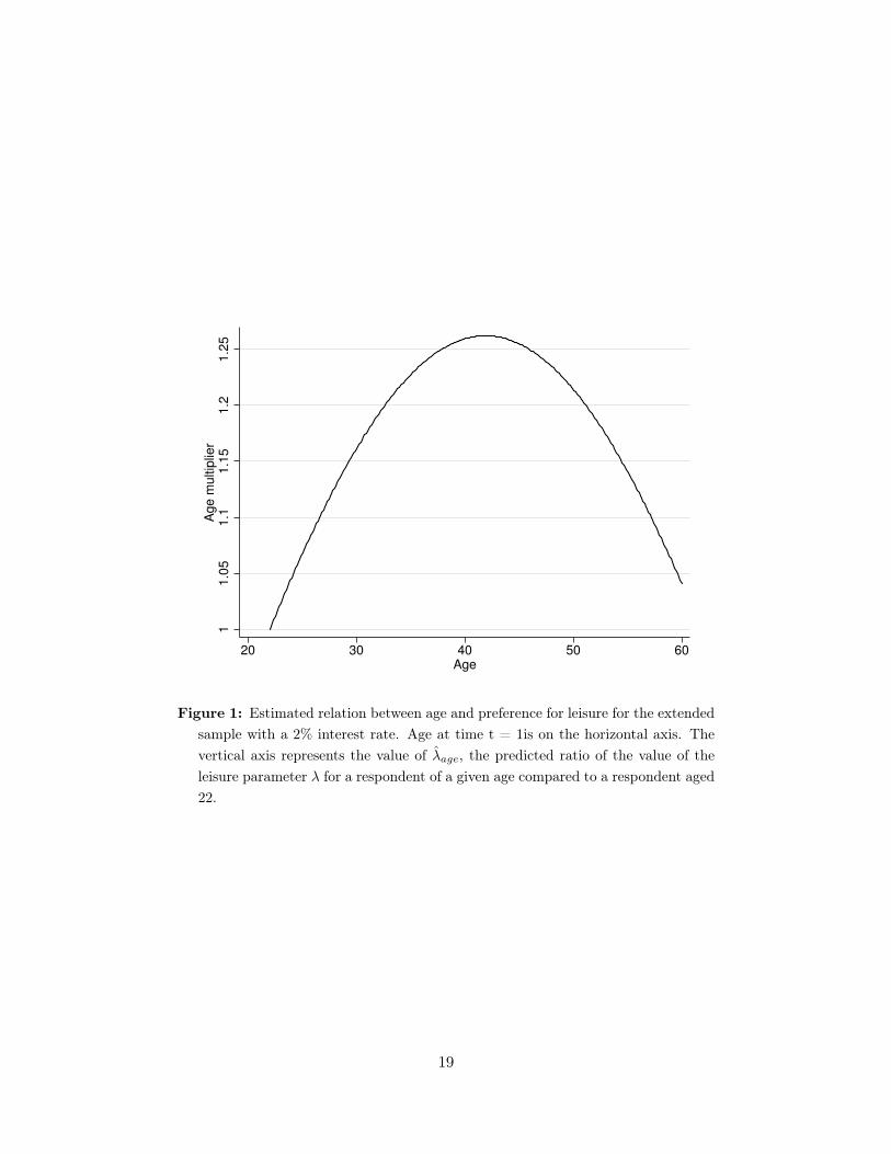
Adding respondents with a partner leads to slightly different conclusions. First, note that thedummy for whether a respondent is in a couple or not is significant at 10%-significance level (withall p-values smaller than 6%). The estimated values of the discount parameter did not change much,staying between 0.95 and 0.97. I now find a significant age trend. The effect of this trend for aninterest rate of 2% and for the extended sample (column 5 in Table 4) is represented in Figure 1.The graph presents:

λ̂age = exp(β̂age/10 (age− 22)/10 + β̂age−sq./1000 (age− 22)2/1000

),

as a function of age. This term can be interpreted as the ratio of predicted value for the leisureparameter of a respondent of a given age compared to a respondent aged 22. Remember that age isa time-constant variable in this model, so that preference for leisure is assumed to be constant fora respondent and not affected by his own aging. We see in the figure that the respondents with thehighest value for leisure are 41.9 years old and have a predicted value of λ almost 25% higher thanrespondents aged 22 with the same observed and unobserved characteristics. While this decreasein value for leisure past 42 may look strange at first sight, a plausible explanation is that we focuson employed respondents and that respondents with high value for leisure are likely to benefit fromearly retirement, leading to a selection effect in older respondents.

5 Simulations

Due to the structural nature of the model, I can use the results to predict the behavior of respondentsunder various scenarios. In this section, I therefore explore the impact of various hypotheses on actualbehaviour, paying particular attention to the possible reaction to a delay of 2 years of eligibility tosocial security.

17

Table 4: Estimation results

Singles only Singles and "half-couples"

1% interest 2% interest 3% interest 1% interest 2% interest 3% interestρ 0.965*** 0.956*** 0.949*** 0.968*** 0.963*** 0.960***

(0.013) (0.011) (0.010) (0.007) (0.006) (0.006)γ0 -0.170** -0.162*** -0.159** -0.117** -0.118** -0.109**

(0.055) (0.058) (0.063) (0.044) (0.047) (0.050)γmen 0.021 0.016 0.011 0.018 0.015 0.010

(0.026) (0.026) (0.025) (0.015) (0.015) (0.015)β0 -1.109** -1.196** -1.410** -0.750* -0.889* -0.981**

(0.543) (0.565) (0.605) (0.430) (0.456) (0.044)βmen 0.130 0.089 0.050 0.096 0.069 0.021

(0.281) (0.279) (0.278) (0.169) (0.172) (0.173)βeduc. med. 0.0.85 0.073 0.059 0.080 0.076 0.071

(0.143) (0.150) 0.160 (0.125) (0.136) (0.143)βeduc. high. -0.011 -0.029 -0.053 0.022 0.015 0.009

(0.133) (0.140) (0.151) (0.123) (0.133) (0.140)βpartner 0.105** 0.107* 0.110*

(0.052) (0.055) (0.058)βpartner×men 0.044 -0.046 -0.049

(0.066) (0.070) (0.074)βage/10 0.042 0.119 0.258 0.163* 0.234** 0.327***

(0.140) (0.153) (0.173) (0.092) (0.101) (0.114)βage-sqr/1000 -0.204 -0.349 -0.582 -0.461** -0.588** -0.738***

(0.336) (0.359) (0.395) (0.216) (0.237) (0.259)

σλ 0.224 0.224 0.227 0.236 0.246 0.256σε 0.117 0.100 0.088 0.197 0.177 0.174

N. Ind. 242 498N 411 828

Standard errors between parenthesesVariable age is age in 2006 minus 22The estimated parameter ρ constrained to be between 0 and 1

18

11.0

51.1

1.1

51.2

1.2

5A

ge m

ultip

lier

20 30 40 50 60Age

Figure 1: Estimated relation between age and preference for leisure for the extendedsample with a 2% interest rate. Age at time t = 1is on the horizontal axis. Thevertical axis represents the value of λ̂age, the predicted ratio of the value of theleisure parameter λ for a respondent of a given age compared to a respondent aged22.

19

5.1 Initial results

Consider the original scenarios proposed to the respondents. For each scenario, I can predict theprobability that a respondent would prefer this scenario over the others. Consider Simulation (1)in Table 5, presenting the average probability to retire at a given age given the heterogenous re-placement rates presented to the respondents. We see that the model predicts large heterogeneityin retirement behavior. While the median and modal retirement age would be 65, the proportion ofrespondents that would choose to retire at 62 or 68 is substantial. Based on the discussion presentedin Section 4.1, it is not surprising that the model predicts about the same proportion of respondentwith preference for retirement at 65 and at 68. However, the share of preference for early retire-ment seems quite high, although not entirely off the mark. The results presented here are in line,at least qualitatively, with the description of the Dutch pension system made by Capretta (2007).However, these results are at odds with Voňková and van Soest (2009), who find a strong preferencefor standard retirement at 65. The difference in results between this paper and theirs could be dueto a different subsample, focus on different stated-preference questions or to the method itself.

The results of this initial simulation are not that interesting per se, given that each respondentfaced a different replacement rate. In what follows, we will consider alternative simulations whererespondents are offered comparable scenarios.

5.2 Reference scenario

For the remainder of the section, I want to offer comparable replacement rates to all respondentsconditional on their retirement at a given age. I start from a common scenario where respondentsare offered a 70% replacement rate of their final income should they retire at 65. This scenariowill serve as a benchmark. I use this information to compute replacement rates under alternativescenarios. One important concept in the determination of the replacement rate is the annuity factorfor a given retirement age r, given by:

A(r) =

100∑t=r

srt(1 + ι)t−r

(9)

Remember that both income at 64 and survival probabilities will vary by respondents, however,subscript i is omitted for ease of presentation.

I assume that pensions are defined in terms of the last wage, as it was the case in the hypotheticalscenarios. Following a description in the OECD guide for pensions, the replacement rate at 65 is

20

Tab

le5:

Simulationresults:

Initialr

esults,a

ctua

rial

neutralityan

ddelayedAOW

(1)

(2)

(3)

(4)

(5)

Hyp

.scena

rios.

Act.n

eutral

Act.n

eutral

Act.n

eutral

Delayed

AOW

(autho

r’s)

(autho

r’s)

(V&

vS,2

009)

Age

Rep.r

ate

%Rep

.ratea

%Rep

.ratea

%Rep

.rate

%Rep

.ratea

%

6152

.47

20.6

53.45

23.6

48.79

18.4

6245

/50/

5530.0

56.31

46.1

56.31

13.6

56.95

14.1

52.48

12.4

6360

.48

10.8

60.80

10.6

56.47

10.1

6465

.03

9.6

65.14

9.1

60.83

9.2

6560

/65/

70/7

535

.670

.00

28.7

70.00

8.9

70.00

8.4

65.59

8.8

6675

.45

8.4

75.00

7.5

70.80

8.7

6781

.45

7.9

81.16

7.4

76.55

8.6

6880

/85/

90/9

534

.388

.08

25.03

88.08

7.4

87.71

6.9

82.91

8.3

6995

.46

6.7

95.17

6.4

89.99

8.0

7010

3.44

5.9

103.53

5.9

97.82

7.4

Meanag

eret.

65.1

64.3

64.5

64.3

64.8

aM

ean

repl

acem

ent

rate

over

the

sam

ple

21

define as 1.75% times the number of years worked, assuming a full career of 40 years. For eachrespondent, I compute the pension wealth at age 65 for a given retirement age given by:

PW (r | 65) = 1.75% (r − 25)A(65)ω64 (10)

Which obviously implies that the value of the pension wealth at 65 for someone retiring at 65 isgiven by.

PW (65 | 65) = 70%A(65)ω64 (11)

The scheme used here has a strange contribution pattern, in the sense that the contribution’s valueat age 65 is the same independently of the age at which it was made, and that hence, the real valuecontributed at each time period is increasing over time. For the sake of comparison with previousstudies, I present here an analysis with a 2% real-interest rate. Given the current economic situationat the time of writing these lines, the real interest rate is probably larger than it should be.

I first want to compute various scenarios under actuarial neutrality, taking into account bothincrease in pension wealth due contribution as time goes by and mortality risk. In the simple settingdeveloped here, the actuarially fair replacement rate is given by:

reprater =(1 + ι)r−65 PW (r | 65)

s65,r A(r)ωr(12)

Note that s65,r is equal to one if r < 65 in our model where there is no mortality between 62 and68.

Simulation (2) in Table 5 presents a simulation of retirement scenarios with the same retirementages that were used before, but with actuarially neutral replacement rates. To simplify the presenta-tion, the replacement rates presented in the table are the average of the replacement rates offered toeach respondent for a given retirement age. On average, these rates are close to the most generoushypothetical scenarios presented to the respondents. These rates would lead to a substantial fractionof the workers retiring at age 62, as almost half of them would be predicted to retire at that ageunder this progression.

To allow for more flexibility in retirement, Simulation (3) allows a respondent to retire at everyage between 61 and 70. The average retirement age in this model is predicted to be 64.5 years old.

While the fact that each respondent receives a different set of replacement rates enforces theconcept of actuarial neutrality, this approach to pension plans is not realistic. An alternative ap-proach would be to use the same replacement rates for every individuals, by using, for instance, the

22

same rates used by Voňková and van Soest (2009). This was done in Simulation (4), allowing us toassess the impact of variations in replacement rates. We see that using this rate leads to an averageretirement age of 64.3, a diminution of 0.2 years, or about two months. It is important to stress thatdespite the seemingly small differences in replacement rates, the heterogeneity in Simulations (2)explains part of the variation in mean retirement age. Results of Simulation (2) would be differentif all respondents were offered the average rates.

5.3 Delayed eligibility to AOW

As discussed above, the current reform in social security should delay eligibility to the pension by 2years, from age 65 to 67. I discussed in Section 2 that public and private pensions in the Netherlandsare often integrated, with the aim to offer a given gross replacement rate to a worker retiring at65. Hence, a shock to social security like the pension reform is not straightforward to implement inmy simulations, as I must make additional assumptions concerning how the occupational pensionsschemes would adjust.

The approach I consider is to interpret the pension reform as a shock on the value of the pensionwealth at 65 that would be absorbed by the occupational pension. I simply remove two years ofsocial security from the pension wealth computed in Equation 11 and compute new replacement ratesbased on Equation 12. Given that the scenarios are expressed in terms of net income, I approximatethe value of social security to be the value received by singles in 2008, and assume that everyonepays on this amount the lowest rate of income tax. This leads to a gross yearly value of 12,718 Euroson which a 33.60% tax is paid. Considering the delay of two years proposed, the net total reductionof PW (65 | 65) is therefore of 16,724 Euros.

This last Simulation, numbered (5), is presented in Table 5. We see, for instance, that theaverage age of retirement increases by 0.3 years, an increase of four months. The impact of thisdelayed payment to social security may look quite small at first glance. It has to be stressed that theNetherlands is a country where individuals accumulate a large pension wealth during their lifetime.According to the most recent OECD report on pension available at the time of writing (cf OECD,2011), the median Dutch man accumulates 12.8 times his net income in pension wealth while themedian Dutch women accumulates 14.6 times her net income. These numbers are among the highestin the countries reviewed in the publication. Thus, a reduction by two year of public pension on thetotal pension wealth does not have an effect as strong as one may expect at first.

An important aspect that must not be overlooked is that the reform is expected to have differenteffects on different individuals. For respondents with lower income, for instance, social security

23

represents a larger share of the pension wealth than for richer individuals. Other factors may affectbehaviour. Younger respondents have more time to adjust their behaviour to a policy change likedelayed eligibility to AOW than older respondents. Even leaving aside differences in preferences, wetherefore predict more important changes in behaviour for older respondents who do not have timeto adjust their consumption over a long period of time. To see how this is translated in terms of thecurrent model, consider Figure 2, presenting scatterplots of the predicted delay in retirement of ourrespondents by income (left panel) and age (right panel).2 We see that at any given level of income

0.5

11

.5P

red

icte

d d

ela

y in

re

tire

me

nt

(ye

ar)

10000 20000 30000 40000 50000Income at t = 1 (Euro)

0.5

11

.5P

red

icte

d d

ela

y in

re

tire

me

nt

(ye

ar)

20 30 40 50 60Age

Figure 2: Predicted delay in planned retirement current income (left panel) and age(right panel), assuming that retirement is fixed at 65. The line is a non-parametricestimate of conditional expectations.

and at any given age, the model predicts a substantial variation in behaviour. In both cases, theaverage trends are correctly predicted.

Another way by which the respondents can adapt to the change in policy is by reducing theirconsumption.3 The structural model used in this paper allows predictions on consumption andsavings. It is therefore possible to predict changes in consumption that would be induced by the

2One respondent with very low income was excluded from the graph. This respondent was predicted to delayretirement by almost two years.

3Given the discrete nature of the model a consumption increase is possible. Given that a respondent can onlyretire once a year, he may decide to delay retirement and to increase consumption. This situation is never predictedby the simulations.

24

policy described above. Let us consider the immediate effect of the reform on consumption. To doso, let us consider the largest variation that the reform could induce in the model at the current timeperiod and for a respondent planning to retire at 65. We compare the predicted consumption beforeand after the reform. This simulation is equivalent to the case of a respondent who did not forecastthe change in policy and who learns of this change at the current time period. Given that mostrespondents seem to anticipate the reform, and given that many of them may delay retirement, thedifference in consumption path is likely to overestimate the observed effect and should be interpretedas an upper bound on predicted consumption change. Consider Figure 3, presenting scatterplots ofthe predicted variation by income (left panel) and by age (right panel). We hardly see a systematic

02

00

40

06

00

80

01

00

0P

red

icte

d c

on

s.

de

cre

ase

at

t=1

(E

uro

)

10000 20000 30000 40000 50000Income at t = 1 (Euro)

02

00

40

06

00

80

01

00

0P

red

icte

d c

on

s.

de

cre

ase

at

t=1

(E

uro

)

20 30 40 50 60Age

Figure 3: Predicted variation of consumption for current year by current income(left panel) and age (right panel), assuming that retirement is fixed at 65.

effect of income on the immediate consumption decline, should retirement be fixed at 65. We alsosee that age is an important factor in the prediction. As we forecasted, older respondents wouldhave to adapt their consumption more than younger. Remember that the current reform of AOWis gradual, and that a full delay in eligibility will only be in effect for respondents aged 55 or more.Note also that a lot of younger respondents would not change their consumption at all. This is dueto the fact that they were prevented to borrow from their pensions, and therefore still plan to enterretirement with a value of accumulated assets equal to 0, as they did before.

To summarize these simulations, it seems that the model predicts that poorer respondents would

25

tend to delay retirement more than higher earners should this reform pass, and to predict that adecrease of consumption is mostly caused by age. There is nevertheless a lot of heterogeneity in thepredicted reaction to this reform.

6 Discussion and Conclusion

In this paper, I used simple questions where respondents are asked to state their preferences toestimate a life-cycle model of retirement and savings. I find that the estimated model yields plausibleestimation of parameters, generally in line with results from the literature, and showed that manyof the problems I faced came from the small sample size or from unavailable data that could easilybe elicited. Respondents seems to answer the questions in a way that is consistent over time, as seenfrom the importance of the random-effects in the analysis. The scenarios I analyze are both easy tounderstand and are in line with the defined-benefit pension plans predominant in the Netherlands,which means that they may relate to them even if they do not have access to such retirement plans.Thus, at first glance, I could not find any obvious reason not to use stated preferences in the analysisof retirement and savings.

Of course, not finding evidence against the use of such data is different from finding evidencein favor of them. The next logical step for this project is to try to compare the predictions of thisestimated model with actual behavior. Failing to reconcile stated and revealed preferences wouldprobably cast doubt on the usefulness of the stated-preference approach. Still, if what people reportis what they plan or hope to achieve, or if it reflects their preferences at a given point in time,there may be some usefulness for the current analysis. A simple and straightforward application isto evaluate how a population may vote on some propositions. Understanding this is important ifpolicy makers want to have the support of the population when proposing pension reforms, notablyin states where votes and referendums are omnipresent. The state of California, for instance, wouldbe a good example.

For the sake of the discussion, let’s assume that stated preferences are a good substitute forrevealed preferences in the study of retirement and savings. In this case, we undoubtedly want toimprove the simple model I presented here. Many of the shortcomings of this research are not due tothe absence of an appropriate theory or to the high cost of eliciting the relevant data, but rather tothe modest sample size available at the time of writing these lines or to the lack of a required pieceof information in the dataset. These problems are not a serious barrier to future research. Elicitingdata of this type is not particularly expensive or challenging, mostly with access to panels such asthe CentERpanel. There are a lot of interesting and important factors that we may want to control

26

for. The structural form dictates well how to augment the model, and, once the new value functionis computed, the econometric model requires only minor adjustments, if any.

Future research topics may include better measurement of risk aversion or may rely on dynam-ically inconsistent preferences (e.g. Laibson, 1997). These last two examples would require cleverlydesigned future scenarios, both easy to understand for the respondents and complete enough toidentify the model used. The fact that researchers can easily vary the assessed scenarios in an exper-imental manner should be a useful tool to actually identify these effects. Household structure andjoint retirement are other interesting topics. I did not take into account, for instance, the numberof children or dependent family members in each household. Again, the decision to exclude thesecharacteristics in the model was mostly driven by the relatively small size of the sample available.We can nevertheless think of an extension to this model that would take these elements into account.In this case, we would probably want to allow the utility from consumption to vary according tothe number of family members, but could think that the value of leisure after retirement should notbe affected (assuming that the children are no longer living with their parents, naturally). Finally,some health related variables, like self-assessed health, should probably be included in the leisureparameter. It would also be interesting to measure perceived spouse’s health, and see how it af-fects retirement plans. Subjective survival probabilities could also be used in order to control forheterogeneity in frailty among the respondents. While these last variables were not available in thedataset, eliciting them does not pose a great challenge. Some of this information will be available inthe 2011 yearly wave of the Pension Barometer Survey, allowing me (and hopefully other researchers)to improve the realism of the model.

References

Beggs, S., J. Cardell, and Others (1981). Assessing the Potential Demand for Electric Cars. Journalof Econometrics 17 (1), 1–19.

Bertrand, M. and S. Mullainathan (2001). Do People Mean What They Say? Implications forSubjective Survey Data. The American Economic Review 91 (2), 67–72.

Bissonnette, L. and A. van Soest (2010). Retirement Expectations, Preferences, and Decisions.Netspar Panel Paper 18, 1–98.

Bissonnette, L. and A. van Soest (2011). The Future of Retirement and the Pension System: Howthe Public’s Expectations Vary over Time and across Socio-Economic Groups. CentER WorkingPaper Series (2011-065 5759).

27

Bovenberg, a. L. and R. H. J. M. Gradus (2008, November). Dutch Policies Towards Ageing.European View 7 (2), 265–275.

Browning, M. and T. F. Crossley (2001). The Life-Cycle Model of Consumption and Saving. TheJournal of Economic Perspectives 15 (3), 3–22.

Browning, M. and A. Lusardi (1996). Household Saving: Micro Theories and Micro Facts. Journalof Economic literature 34 (4), 1797–1855.

Capretta, J. (2007). Global Aging and the Sustainability of Public Pension Systems: An Assess-ment of Reform Efforts in Twelve Developed Countries. Center for Strategic & InternationalStudies: (January).

De Bresser, J. and A. van Soest (2009). Satisfaction with Pension Provisions in the Netherlands -A Panel Data Analysis. Netspar Discussion Paper (DP 10/2009-034).

de Vos, K. and A. Kapteyn (2004). Incentives and Exit Routes to Retirement in the Netherlands.In J. Gruber and D. A. Wise (Eds.), Social Security Programs and Retirement Around the World,Volume I, pp. 461–498. Chicago: University of Chicago Press.

Dominitz, J. and A. van Soest (2008). survey data, analysis of. In S. N. Durlauf and L. E. Blume(Eds.), The New Palgrave Dictionary of Economics. Basingstoke: Palgrave Macmillan.

Euwals, R., A. Eymann, and A. Börsch-Supan (2004). Who Determines Household Savings for OldAge? Evidence from Dutch Panel Data. Journal of Economic Psychology 25, 195–211.

Fok, D., R. Paap, and A. van Dijk (2010). A Rank-Ordered Logit Model with Unobserved Hetero-geneity in Ranking Capabilities. Journal of Applied Econometrics.

Gan, L., M. Hurd, and D. McFadden (2005). Individual Subjective Survival Curves. In D. A. Wise(Ed.), Analyses in Economics of Aging, Volume I, pp. 377–411. Chicago: University of ChicagoPress.

Gruber, J. and D. A. Wise (1999). Social Security and Retirement around the World. NationalBureau of Economic Research, Inc.

Gruber, J. and D. A. Wise (2004). Social Security Programs and Retirement around the World:Micro-Estimation. National Bureau of Economic Research, Inc.

Gustman, A. and T. Steinmeier (1986). A Structural Retirement Model. Econometrica 54 (3),555–584.

Gustman, A. L. and T. L. Steinmeier (2004). Private Pensions and Public Policies. Number 7368,Chapter What Peopl, pp. 57–125. Washington, DC: Brookings Institution.

28

Gustman, A. L. and T. L. Steinmeier (2005). Imperfect Knowledge of Social Security and Pensions.Industrial Relations 44 (2), 373–397.

Hurd, M. D. (1989, July). Mortality Risk and Bequests. Econometrica 57 (4), 779.

Hurd, M. D. (2009). Subjective Probabilities in Household Surveys. Annual Review of Eco-nomics 1 (1), 543–564.

Knoef, M., R. Alessie, and A. Kalwij (2009). Changes in the Income Distribution of the DutchElderly Between 1989 and 2020: A Microsimulation. Netspar Discussion Paper (DP 09/2009-30).

Laibson, D. (1997). Gloden Egg and the Hyperbolic Discouting. Quarterly Journal of Economics 62,443–479.

Lusardi, A. and O. Mitchell (2007, January). Financial Literacy and Retirement Preparedness:Evidence and Implications for Financial Education. Business Economics 42 (1), 35–44.

OECD (2011, January). Pensions at a Glance 2011: Retirement-income Systems in OECD and G20Countries. Paris: OECD Publishing.

Rust, J. and C. Phelan (1997). How Social Security and Medicare Affect Retirement Behavior In aWorld of Incomplete Markets. Econometrica 65 (4), 781–831.

Stock, J. H. and D. A. Wise (1990, October). Pensions, the Option Value of Work, and Retirement.Econometrica 58 (5), 1151–1180.

Van der Wiel, K. (2008, July). Preparing for Policy Changes: Social Security Expectations andPension Scheme Participation. Netspar Discussion Paper (DP 07/2008-025).

Van der Wiel, K. (2009, March). Have You Heard the News? : How Real-Life Expectations Reactto Publicity. Netspar Discussion Paper (DP 06/2009-031).

Van Soest, A., A. Kapteyn, and J. Zissimopoulos (2006). Using Stated Preferences Data to AnalyzePreferences for Full and Partial Retirement. IZA Discussion Paper (WP 2661).

Voňková, H. and A. van Soest (2009). How Sensitive are Retirement Decisions to Financial Incentives:A Stated Preference Analysis. Netspar Discussion Paper (DP 10/2009-036).

Yaari, M. (1965). Uncertain Lifetime, Life Insurance, and the Theory of the Consumer. The Reviewof Economic Studies 32 (2), 137–150.

29

A Assets and debts definitions

I list here the list of assets and debt used in the aggregated definition. This list is the same aspresented in some work I co-authored (Bissonnette and van Soest, 2010). The value of accumulatedasset used in computation is the difference between wealth and debt at the beginning of the year.The element included are as follow:

On the wealth is the sum of the total amounts of the following elements:

1. Checking account

2. Employer-sponsored saving plan

3. Savings accounts

4. Deposit books

5. Savings certificates

6. Single-premium insurance policies

7. Endowment insurance policies

8. Growth funds

9. Bonds

10. Shares

11. All kinds of options

12. Real estate not used for housing

13. Money lent to family

14. Investment not mentioned before

15. Stocks for substantial holding

16. Business equity

The debt is the sum of the total amounts of these elements:

1. Private loans

30

2. Extended lines of credit

3. Debt with mail-order firms

4. Hire-purchase contracts

5. Loans from family and friends

6. Study loans

7. Credit card debts

8. Loans not mentioned before

31