PNNL-22901, Rev.0 EMSP-RPT-016

Prepared for the U.S. Department of Energy under Contract DE-AC05-76RL01830

Statistical Methods and Tools for Hanford Staged Feed Tank Sampling

MS Fountain RT Brigantic RA Peterson

October 2013

PNNL-22901, Rev. 0 EMSP-RPT-016

Statistical Methods and Tools for Hanford Staged Feed Tank Sampling MS Fountain RT Brigantic RA Peterson October 2013 Prepared for the U.S. Department of Energy under Contract DE-AC05-76RL01830 Pacific Northwest National Laboratory Richland, Washington 99352

PNNL-22901, Rev. 0

iii

Executive Summary

This report summarizes work conducted by Pacific Northwest National Laboratory to technically evaluate the current approach to staged feed sampling of high-level waste (HLW) sludge to meet waste acceptance criteria (WAC) for transfer from tank farms to the Hanford Waste Treatment and Immobilization Plant (WTP). The current sampling and analysis approach is detailed in the document titled Initial Data Quality Objectives for WTP Feed Acceptance Criteria, 24590-WTP-RPT-MGT-11-014, Revision 0 (Arakali et al. 2011). The goal of this current work is to evaluate and provide recommendations to support a defensible, technical and statistical basis for the staged feed sampling approach that meets WAC data quality objectives (DQOs).

The three main objectives for this project are described below:

1. Identify current sampling practices, standards, and statistical tools in the U.S. Department of Energy (DOE) complex, nuclear industry, and international community that are applicable to HLW staged feed tank sampling and analysis.

2. Evaluate and apply Pierre Gy’s theory of sampling error terms, EPA recommendations, or other best statistical methods and tools (as applicable) to HLW staged feed tank sampling.

3. Review the basis for the Error Tolerance (Section 7) of the Initial Data Quality Objectives for WTP Feed Acceptance Criteria, 24590-WTP-RPT-MGT-11-014, Revision 0 and execute improvements where recommended and agreed with the One System Integrated Project Team.

Section 2 and Appendix A of the report specifically address the first objective by providing a broad collection of pertinent references and literature summaries, while also generating a considerable number of observations and recommendations (summarized in Section 5) from the review of sampling standards, practices, and statistical tools. High-level conclusions drawn from the objective 1 effort are:

1. Based on both non-DOE and DOE references, the current WAC DQO is consistent with and follows sound principles of statistical sampling and analysis such as sample size (i.e., number of samples) estimation and hypothesis testing, as well as established DQO processes.

2. Currently, no comprehensive radioactive tank waste sampling standard exists; however, a significant number of guidance documents and best practices do exist that are applicable to the topic. Further, formal application of Gy’s sampling theory has not previously been used to conduct any sampling and characterization of radioactive wastes within the DOE complex. However, similar approaches applicable to radioactive tank waste sampling have been used.

3. Physical collection of radioactive tank waste samples has historically been through grab-sampling, either with a point source capture or through coring equipment where the use of a recirculation loop sampling system (currently proposed staged feed sampling system approach) appears to be the first attempt within the DOE complex.

PNNL-22901, Rev. 0

iv

4. A key limitation that impacts application of Gy’s sampling theory in regard to radioactive waste stems from safety concerns (e.g., as low as reasonable achievable [ALARA] standards) and tank sampling constraints due to tank access and sampling configurations. Safety concerns tend to drive sampling plans to collection of the smallest sample mass and number of samples possible to reach a decision.

5. Both non-DOE and DOE references stress the importance of and assume homogenization of bulk waste is required to obtain representative samples if characterization of the entire tank content is required. This is perhaps one of the most significant discoveries of the entire literature review, and indeed, much work has already been done and continues to be done in regard to the means to best sample and qualify Hanford staged feed tank waste prior to transfer to the WTP.

Section 3 covers the second objective in detail by evaluating and applying Pierre Gy’s theory of sampling error terms, EPA recommendations, or other best statistical methods and tools. In particular, the focus was constrained to sampling considerations associated with the Waste Feed Certification Flow Loop and Remote Sampler system as the current means for obtaining samples from the HLW staged feed tanks. A full summary of observations and recommendations was generated and is documented in Section 5. High-level conclusions drawn from the second objective effort are listed below:

1. Gy’s sampling theory promotes a worthwhile attempt to implement correct sampling practices and sampling equipment with the objective of obtaining representative samples of a population of interest by striving to provide all particles with an equal probability of being included in the sample.

2. A formal application of Gy’s sampling theory to staged feed tank sampling is recommended and useful. Although it appears impractical to minimize all error terms, consideration of all potential sampling errors and addressing those most significant errors with practical solutions will reduce sampling uncertainty.

3. The critical importance of properly selecting the most challenging particle density and size as well as having some knowledge as to the expected fraction of the constituent of interest in the bulk solids has been illustrated. In the context of the WAC DQO, it is recommended that further evaluation of the application of Gy’s formula to estimate the appropriate sample solids mass for sample planning be conducted and included in the revised WAC DQO.

4. The potential for large particles (e.g., >310 m) to dramatically influence the impact of Gy’s grouping and segregation error and fundamental error suggests mechanisms to control them need to be investigated if sampling for large particles are of concern. One option is the application of a particle size reduction technology (e.g., a jet mixer pump grinder) to reduce the upper particle size basis significantly, thus providing more favorable conditions to collect samples which represent all particle sizes.

5. Ideally, for Hanford staged feed tank sampling, all of the sampling errors would be minimized or zero, resulting in a sampling error that is as close as is achievable to the fundamental error, which represents the minimum sampling uncertainty that one could achieve. This scenario is unrealistic given the limitations of the staged feed tank mixing system (e.g., non-homogenous mixing), the application of ALARA principles, and the sampling equipment design. However, additional testing

PNNL-22901, Rev. 0

v

to measure the actual system capabilities could result in improved mixing/sampling, a relaxation of sampling objectives, and/or selection of alternate control strategies.

Section 4 covers the third objective in detail by reviewing the basis for the Error Tolerance (Section 7) of the Initial Data Quality Objectives for WTP Feed Acceptance Criteria, 24590-WTP-RPT-MGT-11-014, Revision 0 (Arakali et al. 2011). This review was expanded to also include the Decision Rule (Section 6) and Sampling Design (and Section 8) in the WAC DQO. The focus was to evaluate and then to identify any potential issues and provide recommendations for improvement. A full summary of observations and recommendations is provided in Section 5. High-level conclusions drawn from the objective 3 effort are:

1. The current WAC DQO Section 7 ‒ Error Tolerance and Section 8 ‒ Sampling Design are consistent with sound statistical sampling methods contained in the literature from both non-DOE and DOE sources. The decision rules provided in Section 6 – Decision Rule are sufficient as inputs to statistical methods (i.e., hypothesis test) to make an acceptance decision for each of the constituents in Table 4-1.

2. It is recommended that a method known as guard banding be applied to provide additional insight related to sample size and action limit implications (Ellison and Williams 2007).

3. A time duration for the sample collection campaign should be specified (e.g., collect 10 samples over a 20-hour period) to minimize the influence of the periodic heterogeneity fluctuation error (CE3) due to the influence of the rotating jet mixer pumps. The concept of a random time interval for collecting each of the 60 increments that form a single composite sample should also be included.

4. More details should be provided on how to calculate the number of additional samples needed if an action limit is exceeded. In summary, the number of additional samples required should be based on the measured sample mean and sample standard deviation for each constituent that does not meet the WAC. These results can then be used to estimate the sample size per the Section 7-Error Tolerance methodology.

5. More details should be provided for the sampling design step that discusses if the calculated number of samples is 10 or less; then analyze the remaining samples. For instance, in this case, analyze the required number of additional samples and then conduct the evaluation using the same decision rules/hypothesis test methods. The sample mean and standard deviation for the hypothesis test should be based on the measured results for all the samples analyzed, including the original set of three samples.

PNNL-22901, Rev. 0

vii

Acknowledgements

The authors wish to gratefully acknowledge and thank the following staff who contributed to the technical content and review of this report: Dave Rector (peer reviewer), Rick Shimskey (technical reviewer), Casey Perkins (technical reviewer), Cary Counts (technical editor), Bill Dey (quality engineer), Mona Champion (project office), Claire Longo, Patricia Stauffer, Young Hong.

PNNL-22901, Rev. 0

ix

Acronyms and Abbreviations

AE acceptance error

ALARA as low as reasonably achievable

ALR air-lift recirculating

ASTM ASTM International (formerly the American Society for Testing and Materials)

BVEST Bethel Valley Evaporator Service Tanks

CE2 long-range heterogeneity fluctuation error

CE3 periodic heterogeneity fluctuation error

CFL/RS Waste Feed Certification Flow Loop and Remote Sampler

CITAC Cooperation on International Traceability in Analytical Chemistry

CSL criticality safety limit

CV critical velocity

DE delimination error

DOE U.S. Department of Energy

DQA Data Quality Assessment

DQO data quality objective

DST double-shell tank

DU decision unit

DWPF Defense Waste Processing Facility

EE extraction error

EPA U.S. Environmental Protection Agency

FE fundamental error

GAAT Gunite and Associated Tanks

GEM geostatistical error management

GSE grouping and segregation error

HLW high-level waste

IAEA International Atomic Energy Agency

IHLW immobilized high-level waste

ILAW immobilized low-activity waste

INL Idaho National Laboratory

ISM incremental sampling methodology

ISO International Organization for Standardization

ITRC Interstate Technology and Regulatory Council

PNNL-22901, Rev. 0

x

LDUA Light Duty Utility Arm

MVST Melton Valley Storage Tanks

OE overall estimation error

OHF Old Hydrofracture Facility

ORNL Oak Ridge National Laboratory

PE preparation error

PNNL Pacific Northwest National Laboratory

PuO plutonium oxide

QAPP Quality Assurance Project Plan

RSD relative standard deviation

SRNL Savannah River National Laboratory

SRS Savannah River Site

TE total error

UCL upper control limit

UDS undissolved solids

WAC waste acceptance criteria

WIPP Waste Isolation Pilot Plant

WTP Hanford Tank Waste Treatment and Immobilization Plant

PNNL-22901, Rev. 0

xi

Contents

Executive Summary ..................................................................................................................................... iii 

Acknowledgements ..................................................................................................................................... vii 

Acronyms and Abbreviations ...................................................................................................................... ix 

Figures ....................................................................................................................................................... xiii 

Tables ......................................................................................................................................................... xiii 

1.0  Introduction ...................................................................................................................................... 1.1 

1.1  Objectives ............................................................................................................................... 1.1 

1.2  Methodology .......................................................................................................................... 1.2 

1.3  Success Criteria ...................................................................................................................... 1.2 

1.4  Quality Requirements ............................................................................................................. 1.2 

1.5  Definitions .............................................................................................................................. 1.2 

1.6  Organization of Report ........................................................................................................... 1.4 

2.0  Summary of Sampling Standards, Practices, and Statistical Tools .................................................. 2.1 

2.1  DOE Sampling Standards and References ............................................................................. 2.3 

2.1.1  General DOE References .......................................................................................... 2.3 

2.1.2  National Laboratory References ................................................................................ 2.3 

2.2  Non-DOE Sampling Standards and References ..................................................................... 2.4 

2.2.1  EPA References ......................................................................................................... 2.4 

2.2.2  International References ............................................................................................ 2.6 

2.2.3  Other Non-DOE References ...................................................................................... 2.7 

3.0  Evaluation and Application of Gy’s Sampling Theory .................................................................... 3.1 

3.1  Overview of Gy’s Sampling Theory ...................................................................................... 3.1 

3.1.1  Gy’s Sampling Errors ................................................................................................ 3.2 

3.1.2  Criticism of Gy's Sampling Theory ........................................................................... 3.5 

3.2  Controlling Gy Errors ............................................................................................................. 3.5 

3.2.1  Fundamental Error ..................................................................................................... 3.6 

3.2.2  Grouping and Segregation Error ............................................................................... 3.6 

3.2.3  Long-Range Heterogeneity Fluctuation Error ........................................................... 3.7 

3.2.4  Periodic Heterogeneity Fluctuation Error ................................................................. 3.7 

3.2.5  Increment Delimitation Error .................................................................................... 3.7 

3.2.6  Increment Extraction Error ........................................................................................ 3.8 

3.2.7  Preparation Error ....................................................................................................... 3.8 

3.3  Assessment of Hanford Staged Feed Tank Sampling Approach ............................................ 3.8 

3.3.1  Application of Gy’s Error to Hanford Staged Feed Sampling ................................ 3.11 

3.3.2  Minimum Sample Size Equation ............................................................................. 3.15 

3.3.3  Additional Equations ............................................................................................... 3.17 

PNNL-22901, Rev. 0

xii

3.3.4  Particle Size and Solids Density Basis .................................................................... 3.17 

3.3.5  Example Calculation of Minimum Sample Size ..................................................... 3.18 

3.3.6  Calculated Mass Required Versus Proposed Staged Feed Sample Mass ................ 3.19 

4.0  Review and Evaluation of Error Tolerance and Sampling Design ................................................. 4.1 

4.1  Introduction ............................................................................................................................ 4.1 

4.1.1  Summary of Observations ......................................................................................... 4.1 

4.1.2  Summary of Recommendations ................................................................................ 4.2 

4.2  General Review and Evaluation of Select WAC DQO Sections ............................................ 4.2 

4.2.1  WAC DQO Section 6 – Decision Rule ..................................................................... 4.2 

4.2.2  WAC DQO Section 7 – Error Tolerance ................................................................... 4.3 

4.2.3  WAC DQO Section 8 – Sampling Design ................................................................ 4.7 

4.3  Closing Remarks .................................................................................................................... 4.9 

5.0  Observations and Recommendations ............................................................................................... 5.1 

5.1  Observations ........................................................................................................................... 5.1 

5.1.1  Current Sampling Practices ....................................................................................... 5.1 

5.1.2  Evaluate and Apply Gy’s Sampling Theory .............................................................. 5.2 

5.1.3  Review Error Tolerance Section ............................................................................... 5.4 

5.2  Recommendations .................................................................................................................. 5.5 

6.0  References ........................................................................................................................................ 6.1 

Appendix A Sampling Standards, Practices, and Statistical Tools ........................................................... A.1 

Appendix B Visual Sample Plan ................................................................................................................B.1 

PNNL-22901, Rev. 0

xiii

Figures

3.1. Example Coriolis Meter Data Plot Versus Time ............................................................................ 3.13 

3.2. Proposed Random Time Spacing Concept for Increment and Sample Collection ......................... 3.14 

4.1. Guard Band Concept for Sample Size = 3 and Different RSD Levels ............................................. 4.7 

 

Tables

3.1. Summary of Sampling Errors Described by Gy and Control Measures .......................................... 3.4 

3.2. Example DST Tank Geometry and Recirculation Properties ........................................................ 3.10 

3.3. Sampling Errors and Control Mechanisms for Hanford Staged Feed Tanks ................................. 3.16 

PNNL-22901, Rev. 0

1.1

1.0 Introduction

The Hanford Site double-shell tank (DST) system provides the staging location for waste feed delivery to the Hanford Tank Waste Treatment and Immobilization Plant (WTP). Slaathaug (2013) includes WTP acceptance criteria that describe physical and chemical characteristics of the waste that must be certified as acceptable before the waste is transferred from the DSTs to the WTP. The Initial Data Quality Objectives for WTP Feed Acceptance Criteria, (24590-WTP-RPT-MGT-11-014, Rev 0), to be referred to as the waste acceptance criteria (WAC) data quality objectives (DQO), or WAC DQO, for the remainder of this report, currently establishes the type, quantity, and quality of the data required for waste acceptance criteria (Arakali et al. 2011). Given the importance of making these waste acceptance decisions, the current approach to staged feed sampling of high-level waste (HLW) sludge and the associated sampling error tolerances (Section 7 in WAC DQO) warrants further review and evaluation.

Accurate characterization of the waste feed destined to the WTP is vitally important for both safety and system performance. An accurate characterization rests on several important steps and procedures, one of which is sampling. In this case, the goal of sampling and the sampling process is to obtain an accurate estimate of the waste’s characteristics from measuring the samples’ characteristics (EPA 2012). To reach this goal, an appropriate sample size, proper sampling techniques, and proper sampling equipment are necessary. Furthermore, it is also a key to establishing a defensible basis for and estimation of sampling uncertainty. To this end, this research focused on evaluating the current sampling approach and providing recommendations to support a defensible, technical and statistical basis for the staged feed sampling approach that meets the WAC DQO.

1.1 Objectives

The underlying objectives associated with this work, in accordance with DOE-ORP Inter-Entity Work Order task number M0SRV00091-21 and the test plan TP-EMSP-015 (Fountain 2013), are described below:

1. Identify current sampling practices, standards, and statistical tools in the DOE complex, nuclear industry, and international community that are applicable to HLW tank waste sampling and analysis.

2. Evaluate and apply Pierre Gy’s theory of sampling error terms (Pitard 1993), U.S. Environmental Protection Agency (EPA) recommendations, or other best statistical methods and tools (as applicable) to HLW staged feed tank sampling.

3. Review the basis for the Error Tolerance (Section 7) of the “Initial Data Quality Objectives for WTP Feed Acceptance Criteria,” 24590-WTP-RPT-MGT-11-014, Revision 0 (Arakali et al. 2011) and execute improvements where recommended and agreed with the One System Integrated Project Team.

PNNL-22901, Rev. 0

1.2

1.2 Methodology

The methodology used to support the objectives included a thorough review of literature pertinent to sampling and quantifying uncertainty associated with heterogeneous wastes, including relevant documents from throughout the DOE complex, as well as from the EPA, international references, and various other non-DOE references (e.g., from industry). Next, a technical evaluation of the current approach to staged feed sampling of HLW sludge to meet the requirements of the WAC was conducted. Finally, a subsequent application of the best statistical methods and tools to provide recommended improvements to Sections 6, 7, and 8 of the WAC DQO document (Arakali et al. 2011) was developed.

1.3 Success Criteria

The success of this work was linked to adequately addressing the three objectives listed in Section 1.1. A secondary intent was to provide insight into and guidance for answering the following four key questions:

1. How should the probability distribution, variability for compositional parameters, and overall uncertainty be determined?

2. Is the current practice of statistical sampling in the DOE complex comparable with EPA recommendations and Gy’s sampling theory?

3. Are Gy’s sampling error terms (as interpreted by Pitard) the same, similar, or different when compared to error terms or sources considered for staged feed tank sampling?

4. How do we define sample representativeness in relation to mixing, sampling, subsampling, and measurement?

The content and delivery of this report satisfies the success criteria established for this work.

1.4 Quality Requirements

A graded quality assurance approach was used for this task performed under the U.S. Department of Energy EM-ORP Support Program. The work activities performed in this task were conducted in accordance with the QA-EMSP-001, Environmental Management Support Program Quality Assurance Plan at the Basic Research technology level. This work was conducted in accordance with best laboratory practices (NQA-1-2000-based) as implemented in work flows, work controls, and subject areas in Pacific Northwest National Laboratory’s (PNNL) standards-based management system (How Do I? website).

1.5 Definitions

Key definitions of terms used in this report are listed below. Unless specified otherwise, all of these key terms are from the Interstate Technology and Regulatory Council document Incremental Sampling Methodology (ITRC 2012).

PNNL-22901, Rev. 0

1.3

Accuracy – The degree of closeness of measurements of a quantity to its actual (true) value in the bulk or lot.

Action level – The generic term applied to any numerical concentration value that will be compared with environmental data to arrive at a decision or determination about a potential contaminant(s) of concern (from survey through remediation) or for a user-defined volume of media using environmental sample data.

Bias – The tendency for a measurement to consistently over- or underestimate the actual (true) value. Together, bias and precision (defined below) determine accuracy.

Composite sample – A sample composed of two or more increments, which generally undergoes some preparation procedures designed to reduce the variance in the errors associated in obtaining a measurement from the combined sample.

Data quality objective – A qualitative and quantitative statement derived from the process that clarifies technical and quality objectives, defines the appropriate type of data, and specifies tolerable levels of potential decision errors that will be used as the basis for establishing the quality and quantity of data needed to support decisions.

Increment – A portion of the sampling unit that is collected with a single operation of a sampling device and combined with other increments to form a composite sample.

Laboratory replicate sample – A sample that is split into subsamples for analysis at the laboratory.

Precision –A measure of reproducibility.

Relative standard deviation – The arithmetic standard deviation of a sample divided by the arithmetic mean of a sample.

Replicate (duplicate) sample – One of the two or more samples or subsamples obtained separately at the same time by the same sampling procedure or subsampling procedure.

Sample – For statisticians, a set of observations collected from a population. For field investigators, it is the mass/volume of material obtained from a sampling unit (i.e., consisting of multiple increments). For laboratory technicians, the sample is all the material delivered to the laboratory in a container collected by the field crew.

Sampling error – Anything during sample collection and handling that causes the measured properties of sample to deviate from the properties of the population.

Standard deviation – Measure of the dispersion of imprecision of a sample or population distribution expressed as the positive square root of the variance and that has the same unit of measurement as the mean.

PNNL-22901, Rev. 0

1.4

Statistics – Function of the sample measurements; for example, the sample mean or standard deviation. A statistic usually, but not necessarily, serves as an estimate of a population parameter. A summary value calculated from a sample of observations.

1.6 Organization of Report

The remainder of this report is organized according to the objectives presented in Section 1.1. Specifically, Section 2 provides a review of current sampling practices, standards, and statistical tools in the DOE complex, nuclear industry, and international community pertinent to HLW staged feed tank sampling and analysis. Section 3 provides a detailed evaluation and application of Gy’s sampling theory to HLW staged feed tank sampling. Section 4 presents a review of the Error Tolerance (Section 7), Decision Rule (Section 6), and Sampling Design (Section 8) of the WAC DQO. Finally, Section 5 presents a summary of observations and recommendations from this effort.

PNNL-22901, Rev. 0

2.1

2.0 Summary of Sampling Standards, Practices, and Statistical Tools

This section contains a summary of current sampling practices, standards, and statistical tools used in the DOE complex, nuclear industry, and international community that are applicable to HLW tank sampling and analysis from the standpoint of error tolerance and sampling design. The summary is based on a more exhaustive literature review of appropriate sources contained in Appendix A. The literature review focused on references relating to sampling standards and practices within the DOE complex and non-DOE sources. In total, 51 different references were reviewed. Each of these references and a short summary of key information found in them are provided in Appendix A. In the review, special attention was put on identifying sources that cover some aspect of Gy’s sampling theory (Pitard 1993). It turns out that there are indeed several references to and mention of Gy’s sampling theory in non-DOE standards, but none focus specifically on radioactive tank waste. Conversely, there were only a few sources identified that specifically mention Gy’s sampling theory within the DOE complex, but these were limited in depth and scope (Leung et al. 2012, Hamm et al. 2007) or were focused on testing platforms (Kurath 2012). Hence, in this regard, this report is one of the first attempts to formally and specifically address Gy’s theory of sampling and potential application for characterizing tank waste at Hanford.

Another upfront point worth mentioning is that, in any statistical analysis, one would always prefer more samples in order to increase confidence in decisions based on the resulting sample statistics. However, in dealing with high-level radioactive waste, obtaining a large number of samples usually is not practical (Ferryman et al. 1998). For instance, remote sampling techniques must be used because of radiation dose concerns while sampling the tank contents. In turn, the samples themselves will require appropriate shielding for handling, transport, and storage (ASTM C1751-11) (ASTM 2011). This underlying safety need is a driving theme behind the current WAC DQO and limitations in characterizing the contents of the waste tanks and associated uncertainties.

An acceptable procedure has to be … capable of implementation in such a way as to be safe to the workers involved and the public at large. An unachievable sampling/decision procedure might result in greater danger to the public than a more modest achievable procedure [EPA 1992a].

A high-level summary of the literature reviewed indicates the following:

Based on both non-DOE and DOE references, the current WAC DQO is consistent with and follows sound principles of statistical sampling and analysis such as sample size (i.e., number of samples) estimation and hypothesis testing, as well as established DQO processes.

Physical collection of radioactive tank waste sample has historically been through grab-sampling, either with a point source capture or through coring equipment.

Both non-DOE and DOE references acknowledge the importance of accounting for sources of uncertainty, and to a lesser extent potential errors in sampling that may lead to these uncertainties, in waste characterization. The need to quantify these uncertainties is emphasized for making decisions that are based on some specified level of confidence.

PNNL-22901, Rev. 0

2.2

Some opposing conclusions exist in some of the references, indicating that analytic uncertainty dominates sampling uncertainty and vice versa. Hence, at this point and as contained in the WAC DQO, both of these contributions must be considered and quantified in regard to waste analysis characterization and subsequent transfer decisions. That is, the WAC DQO acknowledges and uses both a sampling relative standard deviation (RSD) and an analytical RSD that are combined to obtain an overall RSD. For a specified confidence level and power, this overall RSD is then used for estimating the number of samples needed as a function of potential measurements for each constituent of interest.

Many of the non-DOE references do mention Pierre Gy’s sampling theory, but they are predominantly focused on environmental sampling, and specifically on solids and soils, as this was the origin of Gy’s sampling theory and methods.

Until just recently in a report by Lueng et al. (2013), DOE references contain no specific mention or use of Gy’s theory; however, there is a substantial acknowledgement and formal treatment related to sampling uncertainty and ways to quantify it, along with associated implications.

Furthermore, consistent with the various references that were reviewed, direct correspondence during the project with scientists and statisticians from DOE National Laboratories Idaho National Laboratory, Los Alamos National Laboratory, Oak Ridge National Laboratory, Pacific Northwest National Laboratory, and Savannah River National Laboratory, as well as international correspondence with United Kingdom's National Nuclear Laboratory and Sellafield, indicated that Gy's theory has not previously been used in conducting any sampling and characterization of radioactive wastes at these sites. But, similar approaches applicable to radioactive tank waste sampling have been used.

A key limitation that impacts application of Gy’s sampling theory in regard to radioactive waste stems from safety concerns (e.g., ALARA standards) and tank sampling constraints due to tank access and sampling configurations. Safety concerns tend to drive sampling plans to collection of the smallest sample mass and number of samples possible to reach a decision.

There also is significant amount of statistical terminology used throughout the DOE complex that has similar counterparts in Gy’s theory, which indicates that some parallels with Gy’s theory are already in place. Indeed, some key important means touted by Gy to reduce sampling uncertainty are already part of the current WAC DQO sampling design (e.g., collecting many smaller increments to form a single, larger-volume composited sample for subsequent laboratory analysis).

Both non-DOE and DOE references stress the importance of and assume homogenization of bulk waste is required to obtain representative samples if characterization of the entire tank content is required. This is perhaps one of the most significant discoveries of the entire literature review, and indeed, much work has already been done and continues to be done in regard to the means to best sample and qualify Hanford staged feed tank waste prior to transfer to the WTP.

PNNL-22901, Rev. 0

2.3

2.1 DOE Sampling Standards and References

As provided in Appendix A, DOE references related to sampling standards and practices were divided into 1) general DOE references and 2) national laboratory references. A total of 23 different references were reviewed, and brief summaries of key points from these references are provided below.

2.1.1 General DOE References

Only one general DOE reference that focuses on tank waste sampling was found—DOE Methods for Evaluating Environmental and Waste Management Samples (Goheen et al. 1994). This document is a compendium of methods related to sampling and analytical activities associated with characterizing waste management samples from DOE sites. The document starts with guidance for effective project planning, which should include a thorough review of the DQO process required for all DOE environmental management projects. The document also includes guidance on both appropriate sampling and analytical methods for collecting and analyzing waste samples.

2.1.2 National Laboratory References

Many different reports published by the DOE national laboratories are relevant to sampling standards and practices. As previously mentioned, none of these reports specifically mention or apply Gy’s theory. However, there is significant consensus on and consistency in the proper application of sound statistical methodologies, sample size estimation, and the importance of quantifying and minimizing uncertainty associated with characterizing waste and reported results.

As with non-DOE sources, DOE references discuss the need to develop a comprehensive list of relevant sources of uncertainty and methods to combine each of the uncertainties (i.e., square and sum each uncertainty component) so an estimate of overall uncertainty can be determined (Burchfield 2003). References cite that an appropriate sampling plan must be responsive to the needs for criticality safety and handling concerns including the timeliness in results so correct decisions can be made (Burchfield 2003). The references also point out 1) the need for both adequate tank mixing and proper sampling because the analytical measurements needed for these analyses cannot be performed in situ and 2) that rotating jet mixer pumps can facilitate homogeneity within the tanks.1 There are many different DOE references that point to a suitable preliminary estimated sampling uncertainty (relative standard deviation) of about 10 percent (Burchfield 2003, Piepel et al. 2006, Remund et al. 1995).

DOE reports also indicate that the number of required samples depends on several factors. In short, if waste properties are sufficiently far from decision thresholds relative to heterogeneity and measurement uncertainties, very few samples may suffice for confident decision-making. However, if waste properties are near thresholds, several more samples may be required (Liebetrau et al. 1997).

1 Current waste feed delivery sampling and mixing program results indicate that mixing is not sufficient to completely homogenize the contents of staged feed tanks. The requirement of homogeneity of tank contents has been relaxed in the waste feed delivery sampling and mixing program to only require a representative sample of the stage feed for waste acceptance testing. Successful sampling and qualification with a representative sample without a homogenous tank has not been completed at the time of this report.

PNNL-22901, Rev. 0

2.4

DOE references discuss the need to consider and measure particle size distributions and other physical characteristics associated with solids (e.g., settling velocity, etc.) (Patterson 1999). These references also discuss considering composite samples for all liquid and solid analyses to facilitate homogeneity as has been mentioned previously.

There is one report by Pitard (2013b) that focuses on two major themes associated with Hanford tank waste sampling: 1) a review of sampling correctness, sampling protocols, sampling systems, and proper cleaning/maintenance of the sampling system and 2) chronostatistics analysis. Pitard’s report identifies the following three significant points relevant to the current WTP project:

1. Conducting an evaluation of sample mass and subsample mass when dealing with slurry streams that have suspended particles as in the case of the Hanford tank waste

2. Introducing randomness in the way sample increments are collected (e.g., random time increments of the time stratum) to cope with potential process cycles (e.g., mixer cycles)

3. Initially supporting the Isolok® sampling system based on the chronostatistical analysis completed. for example, Pitard notes, “It is clear that the exiting sampling systems can perform well relative to a loose selected DQO.” However, in regard to this point, Pitard acknowledges limitations on the use of chronostatistics based on the envisioned small number of samples that will be collected.

One observation relates to Pitard’s suggestion (in regard to WTP sampling tests) on the use of at least a 30-mL sample volume from the Isolok® sampler consisting of six stratified random increments. This approach will be met easily by the current sampling plan for staged feed tank sampling (i.e., 300 mL total sample based on compositing 60 increments of 5-mL each). A similar modified random sampling approach is relevant to staged feed tank sampling in which rotating jet mixer pumps produce a cyclic solids concentration in the sample recirculation loop (discussed in Section 3.3.1).

2.2 Non-DOE Sampling Standards and References

As provided in Appendix A, non-DOE sources related to sampling standards and practices were broken out into 1) EPA references, 2) international references, and 3) other non-DOE references. A total of 28 different references were reviewed. A short summary of key points from these references is provided below.

2.2.1 EPA References

EPA references establish the seven-step DQO process that the WAC DQO follows (EPA 1992a). EPA references note the difficulty in characterizing heterogeneous wastes as well as difficulties in obtaining representative samples from such wastes (EPA1992a). Also, sources of uncertainty, and how uncertainty can be increased when sampling heterogeneous material are discussed in these references. Sources of uncertainty include sample collection, transportation and handling, preparation, subsampling, and analysis. The references discuss the issue of bias. In simple terms, bias will cause the mean value of sample data to be either consistently higher or lower than the “true” mean value. Sources of such bias can come from faults in sampling design, sampling procedure, sample preparation, analytical procedure, contamination, losses, other interactions, and inaccurate calibrations. Moreover, when the sampled

PNNL-22901, Rev. 0

2.5

material is heterogeneous, the references indicates that subsampling that favors one type of item over another is an obvious potential source of bias. A compounding issue is that bias in the sampling of heterogeneous materials can be difficult to detect and/or to measure its absence. Finally, the references list many different statistical techniques that are pertinent to heterogeneous waste characterization, as well as thorough overviews of Gy’s sampling theory. This will be the focus of Section 3 of this report.

The references also introduce the concept of sample correctness, which is a property of the material itself and the equipment used to extract the sample (EPA 1992b). In short, a sample is correct when all particles in a randomly chosen sampling unit have the same probability of being selected for inclusion in the sample. The references discuss that “grab samples” lack correctness; therefore, they are biased.

The references provide a discussion on determining the number of samples with an initial sample size (or number) estimate approach, which is expressed mathematically below (EPA 1992b).

/ 0.5 (2.1)

where:

n = number of samples Za = percentile of the standard normal distribution with Type I2 error = a Zb = percentile of the standard normal distribution with Type II3 error = b D = minimum relative detectable difference [in this case, the difference between the action limit and the sample mean] divided by the relative standard deviation

This is exactly the same approach as that used in the WAC DQO.

Regarding sample mass, the references also mentions Pitard’s procedure for determining the particle size/sample weight relationship that should be met to ensure that an unbiased sample of material is obtained for analysis. This also will be discussed further in Section 3.

The EPA references discuss both sampling theory and sampling design as critical elements in sampling (EPA 1999). The references note that Gy’s sampling theory can facilitate collection of “correct” individual samples, while statistical sampling designs enable statistical analyses and reaching conclusions about the waste. To this end, applying the appropriate components of Gy’s theory to Hanford tank waste should facilitate efforts to obtain the correct samples, and the statistical analysis contained in the WAC DQO should be used to make the acceptance decisions. The WAC DQO process for decision on each constituent is to i) obtain a set of samples, ii) analyze the samples and compute the sample mean and standard deviation for the constituent’s measurements of interest, iii) compute an upper confidence limit for the mean based on standard statistical hypothesis test methods and using the appropriate specified confidence levels in the WAC DQO for each constituent, and iv) making a decision or not on acceptance. For example, if the upper confidence limit for the mean exceeds an action limit, the decision would be not to accept (or possible analyze additional samples to narrow the confidence limit).

2 Type I error is defined in statistics as the incorrect rejection of a true null hypothesis (i.e., false positive). 3 Type II error is defined in statistics as the failure to reject a false null hypothesis (i.e., false negative).

PNNL-22901, Rev. 0

2.6

The references discuss the concepts of accuracy and precision in regard to sampling. Accuracy can be achieved by incorporating randomness into the sample selection process and by selecting an appropriate number of samples (EPA 2012). Precision amounts to the degree of reproducibility of results (e.g., analytical measurements). The document also indicates that for heterogeneous wastes, unbiased samples and appropriate precision usually can be achieved by simple random sampling. In the case of Hanford tank waste, mixing and circulation of the waste for sample collection via the Isolok® system is similar to simple random sampling (i.e., assuming the tank is sufficiently mixed so that its contents are homogenous). The references note that the primary objective of a sampling plan for solid waste is to collect samples that will allow accurate and precise measurements of the chemical properties of the waste. Therefore, if sufficient sample mass is collected properly and analytical measurements are sufficiently accurate and precise, the samples will be considered reliable estimates of the chemical properties of the waste.

The references also provide an example of sample collection at randomly chosen times within a time stratum. This will be a recommendation for the WAC DQO contained in Section 5 of this report, Observations and Recommendations.

EPA sources discuss the concept of sample compositing, which is another methodology being employed to sample Hanford tank waste (EPA 1986). Sample compositing involves combining a number of sample increments collected from the same waste. In the case of Hanford tank waste, 5-mL aliquots will be collected to build a full composted sample of 300 mL (this is where collecting the aliquots at randomly spaced points in time over a time stratum can be invoked). EPA sources indicate that the disadvantage of sample compositing is the loss of concentration variance data, but the advantage of compositing is that a more representative (i.e., more accurate) sample can be obtained. A recurring theme emerges; that is, the actual compositing of samples requires homogenization of all component samples to ensure that a representative subsample is used for analysis. The homogenization procedure, and the containers and equipment used for compositing, will vary according to the type of waste being composited and the parameters to be measured.

Finally, EPA references discuss the basic concept that the overall estimation error (OE) in obtained results is the difference between the analytical estimate of the analyte of interest and the true (usually unknown) value of that analyte (Gerlach and Nocerino 2003). This overall error is an aggregate of total sampling error (TE) and the analytical error (AE) as represented below:

OE = TE + AE (2.2)

Furthermore, as will be discussed in Section 3, the TE can be subdivided as well into the seven sampling errors associated with Gy’s sampling theory [i.e., 1) fundamental, 2) grouping and segregation, 3) long-range heterogeneity, 4) periodic heterogeneity, 5) increment delimitation, 6) increment extraction, and 7) sample preparation].

2.2.2 International References

International references reviewed included sources from the ASTM International, International Atomic Energy Agency (IAEA), International Organization for Standardization (ISO), EURACHEM and Cooperation on International Traceability in Analytical Chemistry (CITAC), as well as some references

PNNL-22901, Rev. 0

2.7

from international industrial entities such as Sellafield Limited (the United Kingdom’s equivalent of the Hanford site).

International references discuss techniques used to obtain grab samples from waste tanks containing high-level radioactive wastes and provide guidance on selecting appropriate sampling devices (ASTM 2011). These references also provide an overview of basic principles on sampling-plan design considerations to obtain accurate results from the samples taken. These principles include guidance that are fairly consistent with the WAC DQO and include 1) identifying goals and confidence levels for decisions, 2) identifying locations for sampling and acknowledging that there could be limitations based on tank access, and 3) thoroughly interpreting data/results to include identification of sources of variation in results. This last principle also highlights variations due to heterogeneity that may be due to a combination of several factors (e.g., nature of the solids, mixing, selective settling in the tanks, etc.).

Another international reference (Dobson and Phillips 2006) indicates that, at the Sellafield site (United Kingdom), the mixing system completely homogenizes the tank contents and keeps solids in suspension. This mixing system is used immediately prior to tank sampling operations.

Other international sources note that evaluating uncertainty requires initial consideration of all possible sources of uncertainty (Ellison and Williams 2012). These references indicate that a study will quickly identify the most significant sources of uncertainty and how the value obtained for the combined uncertainty is almost entirely controlled by the major contributions. This implies that a good estimate of uncertainty can be made by focusing on the sources that make the largest contributions. Moreover, potential sources of uncertainty can be further investigated, and methods can be employed to reduce the uncertainty to an acceptable level where possible.

2.2.3 Other Non-DOE References

Additional non-DOE references outside of EPA and international sources also were reviewed. Some significant points from these sources in regard to sampling include the importance of obtaining representative samples, which depends on both the homogeneity of the material being sampled and the sampling method (Bowen and Bennett 1988). In particular, the most effective way to avoid both random error and bias in sampling is to blend the material to a homogenous state before sampling. The references also discuss minimizing the effects of heterogeneity by drawing many increments from the batch and compositing them for analysis, which also is consistent with the current plan for Hanford wastes.

PNNL-22901, Rev. 0

3.1

3.0 Evaluation and Application of Gy’s Sampling Theory

This section addresses the second research objective of this project, which was to evaluate and apply Gy’s theory of sampling error terms (Pitard 1993), EPA recommendations, and other best statistical methods and tools (as applicable) to sampling staged HLW feed tanks. The main emphasis in this section is on Gy’s sampling theory, with application of other potential best methods reserved for later sections of this report. The overview of Gy’s sampling theory was approached primarily in terms of application to HLW feed tank sampling with the current vision and constraints for the sampling engineering design in mind. In particular, the focus was constrained to sampling considerations associated with the remote sampling loop as the current means for obtaining samples from the HLW tanks. For the double-shell tanks (DSTs) at Hanford, the proposed sampling access point is a center riser that supports the feed suction line to a recirculating sampling loop where an Isolok® sampler collects sample increments from the flowing stream.

As alluded to earlier, it also is important to note that the methods developed by Gy were originally intended for the mining industry, and thus, the EPA has recommended these methods as the most applicable guidance to environmental scientists for the correct sampling and subsampling of soils. However, the EPA also indicates that Gy’s sampling theory is applicable to sampling at hazardous waste sites and to successful subsampling of those samples in the analytical laboratory.

3.1 Overview of Gy’s Sampling Theory

The overall premise of the sampling theory postulated by Pierre Gy is to reduce sampling variation by breaking down, understanding, and addressing the components that contribute to the total variation in a property of interest. In the context of Hanford staged feed tank sampling, the goal is to minimize the variation from one sample to another when sampling, subsampling/preparing, and analyzing the chemical and physical properties of interest for acceptance, such as those contained in the WAC DQO Table 4-1, Data Inputs with Action Limits (Arakali et al. 2011). By understanding the potential sources of variation, one can most often minimize these sources of variation, and increase the overall confidence in acceptance decisions.

Other upfront motivations associated with Hanford staged feed tank sampling and aspects that are addressed via Gy’s sampling theory are described briefly below (EPA 1999):

It is important to obtain representative samples in the field and to retain sample integrity throughout analytical procedures as fundamental to the generation of meaningful data.

Heterogeneity presents a particular challenge in sampling particulate materials representatively and is a factor that must be addressed when developing plans for sampling.

Heterogeneity influences interpretation of data and decisions made about actions taken, such as acceptance decisions for waste transfer based on a statistical hypothesis test.

Gy presents practical sampling methods that can be applied to address the challenges identified above.

PNNL-22901, Rev. 0

3.2

3.1.1 Gy’s Sampling Errors

Throughout this report, an emphasis has been placed on the importance of collecting and analyzing representative samples. Potential errors that result from collecting small volumes of material (e.g., 5-mL increments from an Isolok® sampler) that are meant to represent a much larger volume, such as an entire stage feed waste tank, need to be addressed in the design of the sampling plan. This requires an understanding and delineation of all the potential sampling errors that can bias the results. Pierre Gy describes seven basic sampling errors associated with collecting samples, with the primary emphasis on particulate-containing lots.1 He labels these as errors rather than uncertainty because sampling is an “error-generating process” that contributes to the non-representativeness of the sample (Smith 2001). In short, a representative sample is one that has the same properties of the entire lot (or staged feed tank in the context of this report). For example, for a property such as pH, a representative sample would have the same pH as the average pH of the contents of a staged feed tank. Ideally, such a representative sample would have the same exact pH as that of the staged feed tank contents, but for a variety of reasons, the pH of each sample will vary. Minimizing these variations is the ultimate goal of correct sampling principles.

Before discussing Gy’s errors here, it is noted that there are minor differences found in the literature in the terms and specific wording used to define these errors; however, the terms are similar enough to not be a significant issue. As a high-level introduction, the seven major sampling errors are summarized as follows (ITRC 2012) (Smith 2001):

Fundamental error (FE) ‒ The makeup of any solid, liquid, or gas is fundamentally heterogeneous. Gy called this property “constitution heterogeneity.” As a result, no sample will be truly representative of the whole, and sampling variation will occur. In short, the error results from the size and compositional distribution of the particles.

Grouping and segregation error (GSE) ‒ In a material lot, particles of a specific nature may actually be grouped together or segregated from other types of particles. Gy called this property “distribution heterogeneity.” Again, no sample will be truly representative of the whole. In short, the error results from the heterogeneous distribution of particles within the population.

Long-range heterogeneity fluctuation error (CE2) ‒ Almost inevitably, processes vary over time. Consequently, sampling variation occurs because samples taken at different times will have at least slightly different compositions. In short, the error results from changes in properties of the lot across space or over time.

Periodic heterogeneity fluctuation error (CE3) ‒ Some processes shift when, for example, the temperature rises and falls during the day, or when ingredients are added on a periodic basis. Such changes will affect the product’s composition and, thus, introduce sampling variation. In short, the error results from periodic changes in properties of the lot over time.

1 Gy’s sampling theory is applicable to liquid samples as they are heterogeneous from the perspective of atoms, ions, and molecules; however, most of the seven error terms are not applicable and they can all be minimized with relative ease.

PNNL-22901, Rev. 0

3.3

Increment delimitation error (DE) ‒ To obtain a random sample, every part of the material lot must have an equal chance of being selected. However, if the boundaries of the sample are not defined properly, sampling variation will occur. In short, the error results from incorrect shape of the sample or increment selected for extraction from the population.

Increment extraction error (EE) ‒ Even if the sample boundaries are defined correctly, it may not be possible, in practice, to extract the sample from the lot. The error results from incorrect extraction of the sample or increment because the sampling device is not designed correctly (e.g., improper shape, size, and angle of cutter).

Preparation error (PE) ‒ If the integrity of the samples is compromised in any way (e.g., they become contaminated, are not stored properly, or are processed in such a way that analytes are lost), then this final type of sampling variation will occur. In short, the error results from contamination loss or gain due to alteration, evaporation, degradation, cross contamination, mistake, or fraud.

Table 3.1 further summarizes these seven Gy sampling errors, along with the primary factor leading to each of these errors, what the errors result from, and how to control them (ITRC 2012). Additional details on controlling Gy’s error will also be discussed in the next subsection.

As discussed in Section 2, overall error (OE) is defined as a sum of the analytical error (AE) plus the total sampling error (TE). The TE component can be further decomposed into these individual sampling errors using the convenient notation in Table 3.1. Replacing TE with the seven main sampling error components, the OE equation takes the form:

OE = TE + AE = FE + GSE +CE2 + CE3 + DE + EE + PE+ AE (3.1)

The goal then is to minimize each of these individual errors so the OE is minimized. As with PE, it also will be assumed that there will be strict compliance with analytical procedures and methods implemented to minimize AE.

PNNL-22901, Rev. 0

3.4

Table 3.1. Summary of Sampling Errors Described by Gy and Control Measures (Table 2.2, ITRC 2012)

Factor Leading To: Sampling Error Error Results From: How To Control

Compositional heterogeneity

Fundamental error (FE) Size and compositional distribution of the particles

Increase the sample mass and/or reduce the size of the particles

Distributional heterogeneity

Grouping and segregation error (GSE)

Heterogeneous distribution of particles within the population

Increase the mass of the sample or increase the number of increments

Large-scale heterogeneity Long-range heterogeneity fluctuation error (CE2)

Changes in concentration across space or over time

Reduce the spatial interval between samples

Periodic heterogeneity Periodic heterogeneity fluctuation error (CE3)

Periodic changes in concentration over time

Change the spatial and/or temporal interval between samples

Identifying the correct increment geometry

Increment delimitation error (DE)

Incorrect shape of the sample or increment selected for extraction from the population

Use correct sampling plan design and correct sampling equipment that can sample the entire thickness of the population

Shape of the sample extraction device and nature of the soil

Increment extraction error (EE)

Incorrect extraction of the sample or increment because the sampling device is too small

Use correct sampling equipment that does not push larger particles aside, and use correct sampling protocols

Loss or gain of contaminants during sample handling

Preparation error (PE)

Contamination loss or gain due to alteration, evaporation, degradation, cross contamination, mistake, or fraud

Use appropriate sample handling, preservation, transport, and preparation measures

Finally, for completeness, one could equivalently express the sampling errors in terms of variance (i.e., square of the standard deviation, ). In this case, the use of (rather than s, which is typically used for expressing sample standard deviation) implies the standard deviation of the true but unknown population. In particular, equation (3.2) provides the sum of the variances of the seven types of sampling errors to express the overall variance of the sampling error. Again, ideally, all of the sampling errors would be minimized, resulting in a sampling error that is equal to the FE, which is the best one could do. This FE then would be the best expected uncertainty for each property of interest. The uncertainty then could also be expressed as relative standard deviation so that the sample size and power plots contained in the WAC DQO could be used directly. One remaining challenge then would be to estimate uncertainty for non-particulate oriented quantities of interest, such as pH. In this case, one still must estimate uncertainty (i.e., the relative standard deviation) based on experimental results, historical data, modeling, and related methods discussed in the literature review.

PNNL-22901, Rev. 0

3.5

(3.2)

3.1.2 Criticism of Gy's Sampling Theory

Before completing an overview of Gy’s sampling theory, it is appropriate to acknowledge that there is some criticism of the theory. A short recap on some of the issues found in the literature in this regard is provided next. In their paper, “A Critique of Gy’s Sampling Theory,” Dihalu and Geelhoed (2012) indicate that the practical impact and the scientific value of Gy’s work are unquestionably strong. However, the development of new technologies, recent experimental results, and novel insights show that parts of Gy’s sampling theory need to be updated or revised. Their paper provides the following main conclusions:

Gy’s sampling theory fails to provide convincing theoretical and/or experimental proof that two of its major theoretical parts, namely the discrete selection model and the continuous selection model, are compatible and that they do not mutually conflict.

Gy’s rules for the dimensions and operating speeds of sampling tools are based on considerations that are too simplistic, whereas today more realistic discrete element modeling simulation methods are available. When these more realistic methods are applied to the question of sampling tool design, very different conclusions than those discussed by Gy would be expected.

The use of fudge factors to adjust predicted values with the experimental values is a major point of concern with Gy’s theory.

Gy’s sampling theory is at various points in its presentation unnecessarily complex and lacks clarity.

In another paper, Geelhoed (2011) discusses that a crucial part of Gy’s theory deals with the estimation, prediction, and minimization of the variance of the FE using a formula known as ‘‘Gy’s formula.’’ However, in the paper, Geelhoed notes that experimental evidence supports the conclusion that Gy’s formula is inaccurate. The main premise of the argument has to do with Gy’s original assumption related to independent particle selections, which is used in deriving a formula for variance of FE (equation 3.3) as a function of properties of the population from which the sample is taken and the sample mass. Geelhoed states that particle selection may be dependent even if the sampling is correct. Thus, the calculated variance of FE, using Gy’s formula, does not necessarily provide an accurate prediction or estimation of the actual variance of FE (Geelhoed 2011).

3.2 Controlling Gy Errors

To correctly collect samples as defined by Pitard (1993), each of the sampling errors should be addressed. As provided in Table 3.1 one approach would be to examine each of these sampling errors along with appropriate measures that might be taken to control them. In practice, the focus is usually on FE and GSE. However, the other errors can be important if correct sampling procedures and equipment are not used (ITRC 2012). A more detailed assessment of each of Gy’s errors and common control mechanisms is provided below.

PNNL-22901, Rev. 0

3.6

3.2.1 Fundamental Error

As FE results from the size and compositional distribution of particles, it can be reduced by making the diameters of the largest particles smaller (i.e., communition) or by increasing the sample mass (Smith 2001). It is important to note that, of the seven Gy sampling error components, FE is the only subsampling error that can be estimated before analysis (Gerlach and Nocerino 2003). As provided below, this error is the exception because it is an error that is inherent to the material and not to sampling or analytical procedures. The FE error is assessed on the probability of sampling a material based on shape, density, dispersion, concentration, and particle size.

FE is associated primarily with the particulate matter of interest that comprises slurry. The estimation of the variance of FE, or for short, can be regarded as the relative variance of the sampling error obtained under thorough mixing of the tank prior to sampling. as described in Gy’s theory, is considered to be the minimum possible variance obtainable in sampling. For incomplete or partial mixing, the actual relative variance will be higher than this minimum. A formula for estimating when the mass of the sample is small compared to the mass of the entire lot (Msample << Mlot) as follows (Geelhoed 2011):

(3.3)

where f is particle shape factor, g is a size range factor of the particles in the population, l is a liberation factor of the particles in the population, c is a mineralogical composition factor of the particles in the population, D is the typical particle size, and Msample is the dry solids sample mass (or weight). From this equation, one can see that is inversely proportional to the sample mass and proportional to the cube of the particle size (D3). Hence, larger sample masses can reduce this error, but more importantly, small reductions in the bounding particle size (D) can provide greater reductions in FE. This influence is illustrated by an example provided in Section 3.3.5 below.

3.2.2 Grouping and Segregation Error

Generally, grouping and segregation error (GSE) is a combination of grouping and segregation factors. GSE is driven primarily by differences in particle shape, size, and density. However, magnetic and electrostatic properties, moisture content, and affinity for wall adhesion also can contribute to segregation.

The grouping variance is difficult to eliminate, but it can be minimized by collecting many small increments if delimitation, extraction, and preparation of the increments are performed correctly. The segregation influence of gravity and the distribution heterogeneity tend to be the largest contributors to the segregation influence. Homogenization is the key method to reduce the segregation factor. Furthermore, system design, such as vertical piping, can minimize the segregation influence of gravity.

GSE also can be minimized by collecting and compositing numerous small increments into a single sample. Collecting many increments is supported by the Interstate Technology and Regulatory Council (ITRC), which indicates that one approach is to use a sufficiently conservative default number of increments. ITRC defines a sufficiently conservative default number as, “… one that is high enough to result in a representative sample for the majority of cases even when the DU (decision unit—in this case a

PNNL-22901, Rev. 0

3.7

stage feed tank) is heterogeneous” (ITRC 2012). Based on simulation studies and empirical evidence gathered from at a variety of sites, the ITRC recommends a default range of 30 to 50 increments (ITRC 2012). Thus, the proposed composited sample made up of 60 increments exceeds the recommended ITRC default range and, therefore, is a more conservative approach to controlling GSE.

3.2.3 Long-Range Heterogeneity Fluctuation Error

Long-range heterogeneity error (CE2) is a fluctuating and nonrandom sampling phenomenon. It is spatial, can be identified by variographic experiments, and can be reduced by taking many incremental samples to form a larger volume composite sample. According to the ITRC, CE2 may or may not be a relevant error for a sampling design, depending on whether “… knowledge of the contaminant distribution or mean is desired and the spatial dimensions of both have been defined. Gy’s sampling theory assumes that the parameter of interest is the mean, not contaminant distribution” (ITRC 2012). In either case (i.e., contaminant distribution or contaminant mean value), this error is not seen as a significant contribution to the overall error when the spatial dimensions are limited (e.g., fixed batch of tank waste) or the whole lot characterization is represented by mean concentration values for the analytes of interest.

3.2.4 Periodic Heterogeneity Fluctuation Error

Periodic heterogeneity fluctuation error (CE3) is another fluctuation error that is temporal or spatial in character and results from cyclical changes. An example from the ITRC is a cyclical change in the time for measuring the nitrogen concentration in a field over several growing seasons. If sampling is always conducted at the beginning of the growing season (when nitrogen levels were highest), a misleadingly high value would be reported for the average nitrogen concentration for the entire year. As with CE2, CE3 is an issue only if it causes an inaccurate estimate of a mean for a defined area and, as in this case, for a defined period of time (ITRC 2012).

This is a potential error that could result from the cyclic nature associated operations like rotating jet mixer pumps. However, periodic heterogeneity error can be minimized by correctly compositing samples (EPA 1999). For example, to counter this potential, one could use of a random temporal interval between sample collections, as well as the interval between collections of composited increments. A more detailed explanation of this approach is provided in the context of staged feed tank sampling in Section 3.3.1.

3.2.5 Increment Delimitation Error

Increment Delimitation Error (DE) results from an inappropriate sampling-program design and the wrong choice of equipment for sampling. It is caused by is using an incorrect shape for the sampling device that removes each increment from the population. It also can be caused by the incorrect use of a correct sampling device. In Gy’s theory, a sampling tool that increases DE is termed “incorrect,” and one that reduces DE is called “correct” (ITRC 2012). There is a significant portion of Gy’s theory centered on designs associated with the size/shape of sampling tools to minimize bias. The issue is that, depending on the sample device, some particles have a greater chance of being included in the sample/increment than others. A specific example is subsampling with a rounded scoop that preferentially gathers particles from the top of a soil layer (i.e., the layer that may also tend to have the larger particles). In contrast, a

PNNL-22901, Rev. 0

3.8

rectangular scoop is a more inclusive tool that would gather particles of various sizes consistently throughout the soil layer (ITRC 2012).

3.2.6 Increment Extraction Error

Like DE, increment extraction error (EE) also can result from the use of an incorrect sampling device. However, EE is not only a function of the size of the sampling tool, but also the size of the particles and the correct use of the sampling device. This error results from a sampling device that can bias the fragments that are included or excluded from being captured by the device (ITRC 2012). An example provided by the ITRC is a sampling device that is too small so the cutting edge of the tool pushes particles (e.g., larger sized particles) to the side, rather than capturing them in the sample. To reduce the increment extraction error, one suggestion is to use a correct sampling device that has a mouth size at least three times the size of the largest particle (ITRC 2012).

3.2.7 Preparation Error

Preparation error (PE) results from loss, contamination, or alteration of a sample. The ITRC states that PE is “… the sum of errors introduced by analyte loss, cross contamination, or chemical or physical alteration of the sample that biases sample results relative to the true mean” (ITRC 2012). Some of these errors can be controlled by traditional quality assurance and quality control procedures, such as sample preservation, holding times, and the use of blanks. The potential for preparation error is definitely important to consider and acknowledge in regard to Hanford tank waste sampling and characterization. However, for this report, it is assumed that the quality procedures mentioned above (many of which are highlighted in the references reviewed in Appendix A) are adequate and strict compliance is maintained to minimize this error.

A general assessment of each of Gy’s errors and common control mechanisms as they relate to slurries was provided above. Next, the actual proposed staged feed sampling design and operation will be discussed followed by the application of Gy’s errors directly to staged-feed sampling of HLW.

3.3 Assessment of Hanford Staged Feed Tank Sampling Approach

The U.S. Department of Energy, Office of River Protection (DOE-ORP) mission includes tank waste retrieval, treatment, disposal, and tank farms closure activities. Waste retrieval (from tank farms) and feed delivery to the WTP requires prequalification sampling and critical velocity (CV) measurements in accordance with ICD 19 - Interface Control Document for Waste Feed (24590-WTP-ICD-MG-01-019, Rev. 6). The staged feed also must meet the WAC provided in 24590-WTP-RPT-MGT-11-014 (Arakali et al. 2011) prior to delivery to WTP.

The proposed tank farm feed delivery involves movement of Hanford waste from single-shell tanks and DSTs into specifically selected DSTs that serve as WTP feed staging tanks. The proposed full-scale staged feed tank transfer protocol includes seven consistent batches of 145,000 gallons each to HLP-22 (pretreatment), while mixing, and the last, partial transfer of 76,000 gallons that will leave a 198,000 gallon heel (approximately 72-in. in depth) in the feed staging tank for the next cycle (Duignan et al. 2012).

PNNL-22901, Rev. 0

3.9

The effective collection of HLW prequalification samples for analysis and CV-measurement data is the responsibility of the Tank Operations Contractor and is currently proposed to occur via the Waste Feed Certification Flow Loop and Remote Sampler (CFL/RS) system (Carlson et al. 2013). The CFL/RS system is designed to be mobile and deployable at various DSTs.

The CFL/RS system is integrated into a mixing and sampling process composed of two rotating jet mixer pumps, a slurry transfer pump, and a recirculation loop pumping HLW slurry from the DST pump pit, through the CFL/RS system, and back to the DST through a riser. The CV of the slurry is determined by adjusting velocity and monitoring for settled solids at the bottom of the pipe using an ultrasonic pulse-echo system mounted in a straight horizontal section of 3-in.- diameter pipe. It must be demonstrated that the CV is less than 4.0 ft/sec in a nominal 3-in.-diameter pipe where CV (in this case) is interpreted as the point in which solids stop moving and remain stationary on the bottom of the pipe. A remotely operated Isolok® sampler mounted perpendicularly on a vertical section of pipe is located downstream from the ultrasonic pulse-echo system CV sensor. The Isolok® sampler takes 5-mL samples through a plunger-type sample collection shaft. Current estimates of the sample volume for HLW WAC sample analysis is 300 mL which would require a minimum of 60 sample increments to obtain the target sample volume. The 300-mL sample volume basis assumes 30 g of solids are needed to complete the required analyses, and the solids concentration is assumed to be 100 g/L.

The ability of the tank farms waste feed delivery system to mix and sample HLW feed to meet the WTP WAC is currently under evaluation using two geometrically scaled tanks and a full-scale remote sampler demonstration system (Lee 2012a, Lee 2012b, Lee 2012c). Washington River Protection Solutions, the current Task Operations Contractor, is conducting both small-scale mixing demonstration and remote sampler demonstration testing with realistic simulants to provide an initial estimate of total sampling errors associated with waste feed delivery acceptance. These error values were used in the Initial Gap Analysis (Leung et al. 2012) which satisfies DNFSB 2010-2 Implementation Plan Commitment 5.5.3.1. The ultimate goal of the testing program is to predict the mixing, transfer, and sampling performance for large and dense particulate solids in a full-scale, feed staging tank based on batch transfer consistency with pre-transfer samples (i.e., replicating the waste acceptance process). More broadly, this testing program was developed to address tank farm mixing, sampling, characterization, and transfer system capability to meet the expanded requirements associated with DNFSB Recommendation 2010-2.

The remote sampler demonstration system currently being tested by Washington River Protection Solutions was designed with a vertically oriented Isolok® sampler installed on a remote sample recirculation loop. The proposed operations will mobilize the slurry waste material in the 1-M gal tank using two rotating jet mixer pumps, placed 180 degrees apart while the transfer pump (sample recirculation loop inlet) will be approximately centered between the two rotating jet mixer pumps.

The full-scale rotating jet mixer pumps (two proposed per tank) are being designed to rotate at 0.2 rpm, to sustain a flow rate of 5200 gpm from each 6-in.-diameter nozzle, and deliver a 59 ft/s nozzle velocity (Lee 2012a). After some predetermined period of rotating jet mixer pump operations, the tank waste will be drawn through the sample loop inlet (5 inches from the tank bottom), and tank waste will be recirculated at a proposed rate between 90 and 140 gpm. Table 3.3 summarizes the proposed full-scale system parameters for AW-105, an example double-shell staged feed delivery tank that was also used as the basis for some scaled tests investigating solids accumulation. Testing currently is underway to characterize the performance of the mixing and sampling system, investigate distribution of solids during

PNNL-22901, Rev. 0

3.10

mixing and sampling, and identify and address any shortcomings in the proposed design. For the purposes of this report, the authors’ assessment and recommendations for improvements are based on these proposed operating conditions and systems design.

Table 3.2. Example DST Tank Geometry and Recirculation Properties (Lee 2012a)

Property Full-Scale DST (AW-105)

Diameter (in.) 900 Fill Height (in.) 399 Bottom Geometry Flat Fill Volume1 (gal) ~1,100,000

Mixer Jet Pump 1 Location2 Riser-007 270°, 20 ft

Mixer Jet Pump 2 Location2 Riser-008 85°, 20 ft

Mixer Jet Pump Suction Elevation3 (in.) 5±1 Mixer Jet Pump Suction Diameter (in.) 11 Mixer Jet Pump Nozzle Diameter (in.) 6 Mixer Jet Pump Nozzle Elevation3 (in.) 18

Transfer Pump Location2 Riser-012 270°, 3 ft

Transfer Pump Suction Inlet Diameter4 (in.) 2.25-2.40 Transfer Pump Suction Inlet Height4 (in.) 6

Transfer Line Diameter (in) 3.07 (3-in. Schedule 40)

1. Fill volume is determined by linear scaling of the tank diameter and sludge volume height.

2. The reference point for DST locations presented in this table defines 0° as the bottom (241-AW-105) of the tank in a plan view drawing of the tank. Provided distances are design distances from the center of the riser to the center of the tank.

3. Elevation is relative to the tank bottom. 4. The pump suction inlet diameter of the Full-Scale Transfer Pump is under

development and the tabulated value is based on similar transfer pumps used at Hanford to convey waste. The inlet size on the 1:21- scale tank is not geometrically scaled. The resulting inlet size was too small to accommodate the particle sizes targeted.

Waste feed delivery system testing is currently ongoing while recent reports on limits of performance testing for the mixing system and CFL/RS system using various tank waste simulants (Kelly and Lee 2013), solids accumulation (Duignan et al. 2012), and scaled performance (Kelly et al. 2013) have been released. More recently, Wells et al. (2013) assessed measurement data captured to estimate scaling relationships for waste feed delivery tank performance metrics, in particular transfer undissolved solids (UDS) concentration. The work of Wells et al. (2013), as well as other small-scale mixing demonstration work, recently has been focused on addressing “… a key uncertainty in the waste feed delivery system which is the potential variation in UDS transferred in individual batches in comparison to an initial sample used for evaluating the acceptance criteria.” This current strategy does not require homogenous mixing of the staged feed tank to obtain representative samples.

PNNL-22901, Rev. 0

3.11

3.3.1 Application of Gy’s Error to Hanford Staged Feed Sampling

Applying Gy’s particulate sampling error theory to staged feed waste tank sampling offers a consistent and technically sound approach for minimizing TE. Each stage from initial sample collection to analytical analysis has an associated sampling error that has the potential of being composed of the error types presented in Table 3.1. The sampling error directly impacts the uncertainty placed on the required WAC DQO measurement results produced when conducting sampling, subsampling, and analytical analyses on the staged tank waste for feed delivery to the WTP pretreatment facility. However, correct sampling practices attempt to eliminate as many of these error types as possible and minimize the reminder. The discussion that follows assesses the proposed sampling, subsampling, and analytical activities for staged feed waste acceptance sampling relative to the particulate sampling error types established by Gy. Following this, the main focus shifts to determining the minimum sample solids mass required to limit FE, which is based on the particle shape, maximum particle size, maximum particle density, and the concentration of the most challenging particle of interest.

The stage feed sampling system needs to be separated into two distinct operations when applying and assessing sampling relative to Gy error types. The first distinct operation is the staged feed mixing system where two 5200 gpm jet mixer pumps provide mixing energy to the tank slurry in an effort to homogenously mix tank contents and provide an equal probability for constituents to be delivered to the CFL/RS suction inlet, and if correctly sampled, be represented in the composite sample. The second operation is the CFL/RS system where tank slurry is delivered to 3-in. sample loop piping from a suction inlet 5 inches from the tank bottom, recirculated at 90 to 140 gpm, and 5-mL increment samples are collected over some period of time until a 300mL target sample volume is achieved.

Typically, a fundamental assumption would be that the tank waste contents are adequately mixed to provide a representative sample stream to the CFL/RS system. If the source lot (1-million gal DST) for the characterization samples is not mixed in some areas then the material in those unmixed areas have a zero probably of being sampled. This would be a significant violation of a basic premise of Gy’s sampling theory, which is to sample in a manner that provides equal probability of all constituents of interest being captured. The potential inability to adequately mix the staged feed tank will contribute to an overall increase in uncertainty for staged feed characterization between batch transfers. However, with respect to the staged feed sampling for the purpose of meeting the WAC DQO, this should not impact uncertainty within the set of ten composited samples with an implementation of correct sampling practices and equipment. That is, when the effective mixing zone in the tank reaches a steady-state condition, representative samples, of that material sub-population, can be obtained reproducibly. However, these ten composited samples would not truly represent the entire staged feed tank volume or lot.

Previous tank waste-mixing and transfer campaigns using HLW slurries within scaled WTP vessels have reported that initial batch transfers contain a higher solids concentration of the larger and faster setting particulate materials compared to subsequent batch transfers (Meyer et al. 2012, Kuhn et al. 2012). These larger and faster settling particulate materials segregate towards the lower levels of the tank and are pumped out preferentially. That is, as long as there is solids motion on the tank bottom and the solids are not so large and dense they are never seen by the recirculation loop suction inlet during all batch transfers, no solids accumulation would occur. This reported behavior suggests that staged feed tank sampling strategy from the bottom of the DST would provide bounding composite samples (e.g., high solids concentration, bulk density, likely U and Pu concentrations) for the most heterogeneous distributed

PNNL-22901, Rev. 0

3.12

material where other smaller, slower homogenous distributed materials would still be represented appropriately. Further investigation is suggested to evaluate the implementation of this strategy and it is considered outside the scope of this report.

With the simplifying assumption that the staged feed tank is adequately mixed to produce a bounding set of 10 composite samples (for a WAC decision) that actual represent the tank contents influenced by the rotating jet mixer pumps and no solids accumulation occurs, then the sampling error evaluation becomes focused on the CFL/RS system. The discussion that follows focuses on this second operation and the application and assessment of Gy’s error types.

Grouping and Segregation Error: GSE is driven by variations in material properties and is a combination of grouping and segregation factors. The grouping factor, as defined by Gy, can equal any value between 0 and 1 and it represents the ratio between the number of fragments and the size of the groups. The grouping variance contribution is difficult to eliminate, but can be minimized with many small increments collected assuming that the delimitation, extraction, and preparation of the increments is performed correctly. According to the WAC DQO for Hanford, a composite sample will be 300 mL composited from 60 5-mL incremental samples.

The variance of GSE error is driven primarily by the segregation factor due to differences in particle shape, size, and density because the grouping factor is easier to minimize with many sample increments. However, magnetic and electrostatic properties, moisture content, and affinity for wall adhesion also can contribute to segregation. The segregation influence of gravity and the distribution heterogeneity tend to be the largest contributors to the segregation influence. In the case of Hanford tank waste slurry, the broad range in particle shape, size, and density are major contributors to material segregation.

Homogenization is a key operational target for reducing the segregation factor and for minimizing operating conditions that introduce segregation. For example, the CFL/RS system should have the Isolok® sampling location installed on vertical piping to minimize the segregation influence of gravity. Furthermore, CV must be maintained on horizontal piping sections to minimize any segregation error. This latter recommendation is a default requirement of the proposed CFL/RS system to meet the <4.0 ft/s CV in 3-in. piping criterion. In other words, the stage feed slurry must exhibit no deposition on horizontal piping at flow velocities of <4.0 ft/s.

Long-Range Heterogeneity Fluctuation Error: CE2 is a fluctuating and nonrandom sampling phenomenon. It is spatial, can be identified by variographic experiments, and can be reduced by taking many incremental samples to form a larger volume composite sample. As it relates to staged feed sampling, one would be concerned about large dense particles preferentially accumulating or removed during sampling. If the staged feed tank was homogenously mixed and sampling occurred via a recirculation line where no mass would be removed or added to the tank contents, this error would not apply. Furthermore, in the context of the staged feed sampling for the WAC DQO, the lot of tank waste material is fixed in space and time and the set of 10 composited samples will be representative of the sub-lot of material influenced by the rotating jet mixer pumps, yet not necessarily representative of the entire lot due to an actual non-homogenous condition (i.e., concentration gradient). The current mixing and sampling demonstration program results indicate that the contents of the tank are not homogenously mixed and a solids concentration gradient exists as well as solids accumulation. This heterogeneous condition will significantly influence the difference in characterization results between batch transfers,

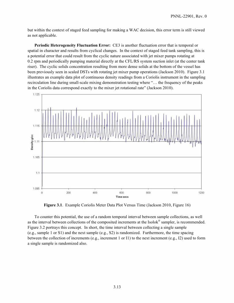
PNNL-22901, Rev. 0

3.13

but within the context of staged feed sampling for making a WAC decision, this error term is still viewed as not applicable.

Periodic Heterogeneity Fluctuation Error: CE3 is another fluctuation error that is temporal or spatial in character and results from cyclical changes. In the context of staged feed tank sampling, this is a potential error that could result from the cyclic nature associated with jet mixer pumps rotating at 0.2 rpm and periodically pumping material directly at the CFL/RS system suction inlet (at the center tank riser). The cyclic solids concentration resulting from more dense solids at the bottom of the vessel has been previously seen in scaled DSTs with rotating jet mixer pump operations (Jackson 2010). Figure 3.1 illustrates an example data plot of continuous density readings from a Coriolis instrument in the sampling recirculation line during small-scale mixing demonstration testing where “… the frequency of the peaks in the Coriolis data correspond exactly to the mixer jet rotational rate” (Jackson 2010).

Figure 3.1. Example Coriolis Meter Data Plot Versus Time (Jackson 2010, Figure 16)

To counter this potential, the use of a random temporal interval between sample collections, as well as the interval between collections of the composited increments at the Isolok® sampler, is recommended. Figure 3.2 portrays this concept. In short, the time interval between collecting a single sample (e.g., sample 1 or S1) and the next sample (e.g., S2) is randomized. Furthermore, the time spacing between the collection of increments (e.g., increment 1 or I1) to the next increment (e.g., I2) used to form a single sample is randomized also.

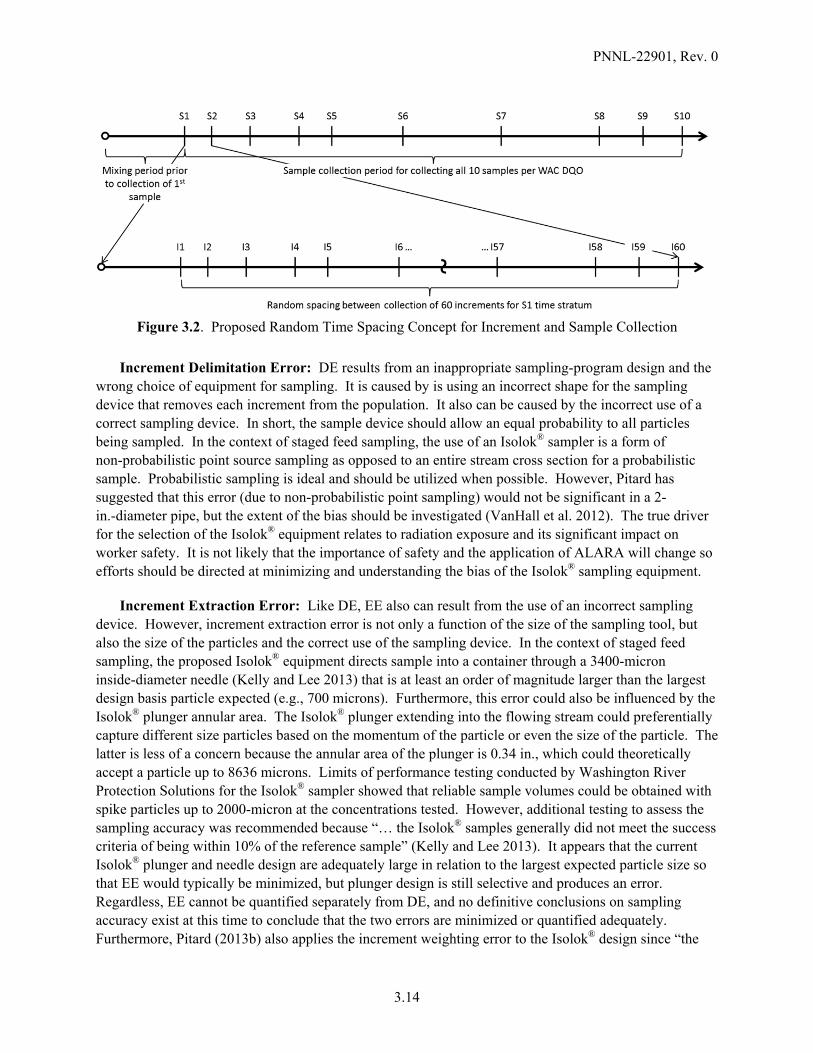
PNNL-22901, Rev. 0

3.14

Figure 3.2. Proposed Random Time Spacing Concept for Increment and Sample Collection

Increment Delimitation Error: DE results from an inappropriate sampling-program design and the wrong choice of equipment for sampling. It is caused by is using an incorrect shape for the sampling device that removes each increment from the population. It also can be caused by the incorrect use of a correct sampling device. In short, the sample device should allow an equal probability to all particles being sampled. In the context of staged feed sampling, the use of an Isolok® sampler is a form of non-probabilistic point source sampling as opposed to an entire stream cross section for a probabilistic sample. Probabilistic sampling is ideal and should be utilized when possible. However, Pitard has suggested that this error (due to non-probabilistic point sampling) would not be significant in a 2-in.-diameter pipe, but the extent of the bias should be investigated (VanHall et al. 2012). The true driver for the selection of the Isolok® equipment relates to radiation exposure and its significant impact on worker safety. It is not likely that the importance of safety and the application of ALARA will change so efforts should be directed at minimizing and understanding the bias of the Isolok® sampling equipment.

Increment Extraction Error: Like DE, EE also can result from the use of an incorrect sampling device. However, increment extraction error is not only a function of the size of the sampling tool, but also the size of the particles and the correct use of the sampling device. In the context of staged feed sampling, the proposed Isolok® equipment directs sample into a container through a 3400-micron inside-diameter needle (Kelly and Lee 2013) that is at least an order of magnitude larger than the largest design basis particle expected (e.g., 700 microns). Furthermore, this error could also be influenced by the Isolok® plunger annular area. The Isolok® plunger extending into the flowing stream could preferentially capture different size particles based on the momentum of the particle or even the size of the particle. The latter is less of a concern because the annular area of the plunger is 0.34 in., which could theoretically accept a particle up to 8636 microns. Limits of performance testing conducted by Washington River Protection Solutions for the Isolok® sampler showed that reliable sample volumes could be obtained with spike particles up to 2000-micron at the concentrations tested. However, additional testing to assess the sampling accuracy was recommended because “… the Isolok® samples generally did not meet the success criteria of being within 10% of the reference sample” (Kelly and Lee 2013). It appears that the current Isolok® plunger and needle design are adequately large in relation to the largest expected particle size so that EE would typically be minimized, but plunger design is still selective and produces an error. Regardless, EE cannot be quantified separately from DE, and no definitive conclusions on sampling accuracy exist at this time to conclude that the two errors are minimized or quantified adequately. Furthermore, Pitard (2013b) also applies the increment weighting error to the Isolok® design since “the

PNNL-22901, Rev. 0

3.15

volume of the Isolok® increment is always the same, regardless of flow rate in the stream to be sampled, therefore the Isolok® is not proportional.” Therefore, it is recommended that additional testing using tank waste simulants be completed including the comparison of non-probabilistic Isolok sampler with a probabilistic reference sampler (e.g. Vezin), in an attempt to bound the magnitude of potential error.

Preparation Error: PE results from loss, contamination, or alteration of a sample. It is first assumed that the quality procedures mentioned above (many of which are highlighted in the references reviewed in Appendix A) are adequate and strict compliance is maintained to minimize this error. Second, the automated sample bottle handling and tracking systems offer a method to minimize this error by removing human error. Finally, the sample flushing protocol is an important aspect that should be acknowledged as a potential source of error and a necessary function to reduce error resulting from cross contamination.

A summary of each of the six Gy’s errors, their applicability to Hanford staged feed tanks, and proposed control mechanisms for the Hanford staged feed tanks is provided in Table 3.3.

The application and assessment of the six error types above leaves only FE. Gy has derived a basis for which FE can be limited to some quantity by properly collecting a minimum sample mass, while all other error types are minimized or eliminated by correct sampling practices and equipment. An example application of this approach is presented in the following subsections.

3.3.2 Minimum Sample Size Equation

Gy’s sampling theory (Pitard 1993) states that the largest particle size fraction that comprises less than 5 wt% of the UDS is also the most challenging to represent in the sample. Thus a sample with sufficient mass to be representative of the largest size fraction, at low solids fraction, will also be representative of all size fractions. A simplified version of Gy’s formula [equation (3.3)], provided by Pitard (2009), illustrates the relationship between the sample mass, the largest size fraction, and variance of the FE through equation (3.4) 1

2 (3.4)

where Ms is the mass of solids in the sample (dry basis), f is a shape factor which is approximately 0.5 for an ordinary spherical particle (f=1.0 for cubes and f=0.1 for flakes), c is the density of the size fraction of interest in g/cm3, dc is the size fraction of interest in cm, ac is the proportion of that size fraction in the total solids lot (e.g., 0.5 weight percent of the UDS content), and is the acceptable or target FE or uncertainty. Pitard (2009) states that this equation holds as a good approximation when MLot > 10MS, the fraction of large particles represent <20 percent of the solids in the lot and ac is less than 30 percent.

Switching and in equation (3.4), highlights that the variance of the FE [ ] is proportional to increased particle density, is inversely proportional to the sample mass, and increases with particle size cubed. Because the largest particle size at low solids fraction is the most challenging to represent, equation (3.4) can be used to determine the minimum required sample size to represent all size fractions in the sample to the required uncertainty target or objective.

PNNL-22901, Rev. 0

3.16

Table 3.3. Sampling Errors and Control Mechanisms for Hanford Staged Feed Tanks

Sampling Error Applicability to Hanford Staged

Feed Tank Sampling Proposed Control Mechanisms

Grouping and segregation error (GSE)

Potential heterogeneous distribution of particles within the tank if not well mixed.

The 300-mL sample will be composited from 60 5-mL incremental samples. Samples collected from a vertical recirculation loop line. Critical velocity will be met in all horizontal piping. Bounding sample strategy to mitigate segregation influence.

Long-range heterogeneity fluctuation error (CE2)

Potential exists for changes in concentration across space or over time. Inadequate mixing could generate solids gradients and non-representative samples of entire tank waste lot.

Well mixed tank and sampling via a continuous circulation loop. Collecting many incremental samples to form a larger volume composite sample.

Periodic heterogeneity fluctuation error (CE3)

Potential exists for periodic changes in concentration over time associated with pumping cycles of the rotating jet mixer pumps used for mixing the tank.

A random temporal interval between samples and the composited increments collected at the Isolok® sampler is recommended.

Increment delimitation error (DE)

Use of the non-probabilistic Isolok® plunger-type sampler is the current methodology envisioned to extract “point” increments from a 2-inch stream.

Initial evaluations and use of the Isolok® “point” sampling have some support. Proper use of the Isolok® is necessary to control error. Maximize point sample cross-section relative to flowing stream cross-section.

Increment extraction error (EE)

Incorrect extraction of the sample or increment because the sampling device is too small.

Proper plunger design (annular area) used on the Isolok® sampler. The proposed needle inside diameter will be at least an order of magnitude larger than the example design basis particle (e.g., 310 microns). The annular area of the plunger much greater than largest anticipated particle.

Preparation error (PE)

Potential exists for contamination, alteration, evaporation, degradation, cross contamination, mistake, or fraud with the samples collected from the waste tanks.

Use sound procedures with strict compliance to their use. Minimizing human error using automated sample bottle handling and tracking system. Implement appropriate sample flushing protocol to minimize cross contamination.

Gy’s formula represents a modeling approach to estimate uncertainty. An alternative empirical approach has been proposed by Lyn et al. (2007) where they estimated a 22.5 percent RSD caused by sampling using an empirical approach compared to a 136 percent RSD using Gy’s modeling approach. The author’s summarized their opinion with the statements “The empirical approach to uncertainty estimation, with the automatic inclusion of sampling within the uncertainty statement, is recognized as generally the most practical procedure, providing the more reliable estimates. The modeling approach is also shown to have a useful role, especially in choosing strategies to change the sampling uncertainty,

PNNL-22901, Rev. 0

3.17

when required” (Lyn et al. 2007). One conclusion that could be drawn from this comparison is that the modeling approach is overly conservative in estimating uncertainty.

3.3.3 Additional Equations

The definition of the solids mass fraction sl in slurry is

≡ (3.5)

where Msl is the slurry mass. The mass fraction of solids can also be calculated from the densities of the slurry (sl), the solids (s), and base liquid (l) (Wills and Napier-Munn 2006) using

(3.6)

The general definition of bulk density is the mass per unit volume represented by

≡ (3.7)

3.3.4 Particle Size and Solids Density Basis

To apply equation (3.4), an estimate of the particle diameter of the coarsest material, defined by the square mesh opening that retains no more than 5 percent of the material, is necessary. In addition, a solid density estimate of this coarse material is needed. An appropriate example source of average bounding waste properties are reported in, RPP-9805, Values of Particle Size, Particle Density, and Slurry Viscosity to Use in Waste Feed Delivery Transfer System Analysis (Jewett et al. 2002), although more recent and improved estimates to these waste properties have been reported (Poloski et al. 2007, Wells et al. 2007, Wells et al. 2011). It is recognized that selection of the particle size and solid density basis is a developing topic so values reported in RPP-9805 are used for an instructive example. RPP-9805 reports the particle size distribution (based on 7 waste tanks) representing the 95 percent confidence limit for 95 percent of the waste tank population as 1 percent is 2 microns, 50 percent is 22 microns, 95 percent is 460 microns, and 99 percent is 700 microns. The more appropriate and less conservative 95 percent confidence upper limit for the tank waste particle size distribution is 1 percent is 1 micron, 50 percent is 11 microns, 95 percent is 210 microns, and 99 percent is 310 microns. Therefore, the 310-micron particle size will be considered the bounding case for the CFL/RS system. Again, this bounding particle size can be disputed; yet, at this time, it currently serves as the WTP system design basis value.

This project report takes the position that, if correct sampling practices are implemented and minimum sample mass requirements (based on this bounding particle size) are met, then any reduction in the upper particle size range will only increase confidence in obtaining characteristic mean values representative of the entire staged feed tank.

The maximum solids density is also an important parameter is estimating the minimum sample mass through equation (3.4). The highest estimated dry solids weighted average density for HLW feeds is

PNNL-22901, Rev. 0

3.18

3.5 g/mL, and this is based on Tank AW-103 (Table 4-2 in Jewett et al. 2002) while the average of the eight tanks is 2.9 g/mL. The 95/95-tolerance limit for the density of true dry solids in HLW tanks was calculated to be 3.9 g/mL. This one-sided 95/95-tolerance limit represents a 95 percent confidence that at least 95 percent of the tanks will have a median dry solids density no larger than 3.9 g/mL. However, the densities were calculated as the weighted averages of the book-value densities of the compounds, and the effective density due to agglomeration is more representative of true conditions. Sufficient data to calculate effective densities with confidence do not exist at this time so estimates were made. The maximum solid density using this approach is reported for tank AY-102 and is 2.68 g/mL, while the average solids density is 2.18 g/mL (Table 4-4 in Jewett et al. 2002). The upper bound value of 3.9 g/mL is not selected as it contains extreme conservatism on an already conservative approach to solids density (i.e., no accounting for agglomeration). In contrast, the approach to estimate effective density due to agglomeration is riddled with insufficient data, and an overall lack of conservatism exists in the average solids density estimate of 2.18 g/mL. The solids density recommended by Jewett et al. (2002) is 2.9 g/mL. In the engineering assessment conducted here, the solids density recommended for use is 3.5 g/mL as it represents a known maximum for which sampling representativeness could be impacted.

3.3.5 Example Calculation of Minimum Sample Size

The sampling methods for the staged feed tank sampling are designed to provide representative samples, the mass of which depends upon several factors as illustrated by the following calculation. For the analysis, a particle with the fastest settling velocity and that is the most challenging to suspend (i.e., largest critical shear stress) is proposed to be used to bound these particle characteristics. However, this selection must be made with a realistic assessment of the properties of interest and their concentration in the bulk lot. For example, particles up to 2000 micron were reliably collected by an Isolok® sampler in recent remote sampler demonstration work (Kelly and Lee 2013). This particle size would be rare and a very low fraction, so not likely an important property of interest. Therefore, it should not be the basis by which the minimum dry solids mass sampling requirement is estimated. A realistic selection of an example challenge particle is assumed to be a 310-micron (0.031-cm) particle with an average solid density of 3.5 g/cm3. Assuming the proportion of this size fraction is 0.05 wt% (0.0005 fraction or 500 ppm) of the UDS, the shape factor has a typical value of 0.5 (Pitard 2013a) for spherical particles, and the required FE uncertainty is 3.5 percent (0.035) (Pitard 2013a, Appendix 2, Table 3) for two-tier sampling of precious metals, the minimum UDS sample mass using equation (3.4) is: . .

. .2 0.031 = 85 g

(3.8)

For the present analysis, tank waste is assumed to contain a maximum of 15 wt% UDS within the slurry. Using the definition of solids mass fraction (equation (3.5)), the slurry (liquid and solids) mass associated with the minimum UDS mass is: 85

0.15 /567

(3.9)

Assuming the average density of all UDS species is 2.9 g/cm3 (Jewett et al. 2002) and the liquid density is 1.0 g/mL, rearrangement of equation (3.6) gives the slurry density as:

PNNL-22901, Rev. 0

3.19

2.9 10.15 1 2.9 2.9

1.1 / (3.10)

The slurry volume using equation (3.7) and containing the minimum UDS mass of 85 g is: 567

1.1515

(3.11)

Thus, this example suggests that approximately 515 mL of slurry with 15.0 wt% UDS (i.e., before addition of flush liquid) must be collected to obtain the minimum solids mass required for a representative sample at 3.5 percent uncertainty (assumes only FE) based on the 310-micron challenge particle at 0.05 wt% (0.0005 fraction) of the UDS content. This example result is believed to be realistic for sampling to test against action limits set in the WAC DQO.

Applying equation (3.4) to the case of a 100-micron, 11.2 g/cm3 PuO particle, at an equivalent fraction (i.e., 500 ppm) and target uncertainty (i.e., 3.5 percent) as the 310-micron particle, highlights the sensitivity of Gy’s formula to particle size. The minimum UDS sample mass using equation (3.4) is:

. .

. .2 0.01 = 9.1 g (3.12)

The estimated minimum solids mass required for the assumed PuO particle is roughly an order of magnitude lower than that of the assumed 310-micron challenge particle. However, decreasing the PuO particle fraction in equation (3.12) from 500 ppm to 50 ppm and all other parameters held constant, the minimum UDS sample mass required is estimated to be 91 g. This is approximately equivalent to the result in equation (3.8).

The above example application of Gy’s formula clearly illustrates the critical importance of properly selecting the most challenging particle density and size as well as having some knowledge as to the expected fraction of the constituent of interest in the bulk solids. In the context of the WAC DQO, it is recommended that further evaluation be conducted regarding the application of Gy’s formula to estimate the appropriate sample solids mass for sample planning. More detailed discussion of the application of Gy’s formula for trace constituents, such as gold, is provided in Chapter 19 of Pitard’s textbook (Pitard 1993), and an updated strategy to address sampling difficulties related to trace constituents is suggested in a more recent journal article by Pitard (2010).

3.3.6 Calculated Mass Required Versus Proposed Staged Feed Sample Mass

The actual HLW sample volume proposed for staged feed analytical analyses to test the WAC is 300 mL. This sample volume is predicted to contain 30 g of UDS based on the assumption of 100 g/L solids concentration. The above example calculation suggests that the minimum sample mass (calculated to be 85.03 g in example) requirement is not being met with the proposed stage feed sampling campaign. Furthermore, Pitard (2013a) generally recommends collecting twice this mass to achieve confidence that the fraction of interest is accounted for in the sample. However, if one rearranges equation (3.4) to solve for , we can estimate the total sampling error if all other six error types are minimized through proper sampling equipment and sampling protocol.

PNNL-22901, Rev. 0

3.20

. .

.2 0.031 = 0.0035 or 0.35 percent variance in FE (3.13)

Taking the square root of the variance of FE provides a predicted relative uncertainty on the order of 5.9 percent assuming all other sampling errors are negligible compared to FE. In general, the proposed sample plan can be successful for materials in relatively abundant concentrations; however, for trace constituents there may be more serious issues.

Pitard (Kelly 2013) provided a grim picture of the minimum sample mass required to represent all Pu particle sizes in a staged feed sample. He estimated a minimum sample mass size of 13.75 kg for 100-μm Pu particles at the 10 ppb level for a 10 percent uncertainty. This example clearly illustrates the material of interest fraction ( ) in the bulk has the most dramatic effect on the estimated minimum sample mass required. Relative confidence in the largest size fraction and solids density generally exists for tank waste; however, the rarity of a trace particle (e.g., Pu) significantly impacts the minimum mass requirement. Because of the uncertainty in the fraction of the material of interest ( ), the best recommendation would be to understand the severity of the influence and collect as much sample mass as tolerable from a safety standpoint.

It is possible that relatively large, dense particles (e.g., Pu) will never see the CFL/RS suction inlet and in such a low proportion of the tank solids that they would not be detectable with the proposed sampling protocol (e.g., 60 5-mL increments collected by an Isolok® sampler). This potential reality has been discussed multiple times by Pitard in his reports to BNI (Kelly 2013; Pitard 2013a, 2013b) and more generally in his journal article on trace constituent sampling (Pitard 2010).

PNNL-22901, Rev. 0

4.1

4.0 Review and Evaluation of Error Tolerance and Sampling Design

This section of the report is focused on the third project objective to review the basis for the Error Tolerance (Section 7) of the Initial Data Quality Objectives for WTP Feed Acceptance Criteria (Arakali et al. 2011).

4.1 Introduction

The Error Tolerance section of the WAC DQO provides an uncertainty evaluation to assess required accuracy and precision for sample collection and analysis, the level of decision error, and the number of samples required to meet a given decision error rate (e.g., confidence level) associated with the WAC DQO action limits. This section was reviewed in detail, along with the associated Section 6, Decision Rule, which outlines the decision rules for the action limits for the constituents contained in Table 4-1 Data Inputs with Action Limits of the WAC DQO, and Section 8, Sampling Design, which provides a step-by-step outline of the current sampling approach. It was important to also review these additional sections as they work hand-in-hand with the envisioned implementation of the statistical methods contained in Section 7. The initial focus was to evaluate the sufficiency of the error tolerance section and then to identify any potential issues and recommendations associated with the sampling design. A summary of key observations and recommendations generated during this review and evaluation are provided below.

4.1.1 Summary of Observations

Following are key observations derived from a review and evaluation of the WAC DQO sections mentioned above:

The current WAC DQO Section 7, Error Tolerance, and Section 8, Sampling Design, are consistent with sound statistical sampling methods contained in the literature from both non-DOE and DOE sources.

The underlying sample sizes (i.e., number of samples1) for confidence levels and power are consistent with standard statistical practices in both non-DOE (e.g., EPA QA/G-9S) and DOE settings (e.g., the Visual Sample Plan developed by PNNL – reference Appendix B).

The sampling design procedures outlined in Section 8, Sampling Design, of the WAC DQO are an appropriate implementation of sequential hypothesis testing, which is also consistent with methods and best practices in both non-DOE and DOE settings.

The decision rules provided in Section 6, Decision Rule, are sufficient as inputs to statistical methods (i.e., hypothesis test) to make an acceptance decision for each of the constituents in Table 4-1. Confidence levels are provided for each constituent (90 percent), with the exception of criticality safety limit requirements which will be evaluated at a 95 percent confidence level.

1 For the remainder of this section, sample size will be synonymous with the number of samples to be collected.

PNNL-22901, Rev. 0

4.2

Some rationale for these confidence levels is provided. How to use the decision rules if action limits are exceeded (e.g., adjust the waste to meet requirements, change the WAC, transfer to an alternative treatment, or continue to store the waste) was clearly stated in Section 6, Decision Rule.

4.1.2 Summary of Recommendations

The following are key recommendations derived from a review and evaluation of the aforementioned WAC DQO sections:

It is recommended that a method known as guard banding be applied to provide additional insight related to sample size and action limit implications (Ellison and Williams 2007). This method is described further below, but in short, a guard band can provide insight into the mean value of the samples that will be required for acceptance of a particular action limit based on the sample size, an assumed variability, and desired confidence level.

A time duration for the sample collection campaign should be specified (e.g., collect 10 samples over a 20 hour period) to minimize the influence of the periodic heterogeneity fluctuation error (CE3) due to the influence of the rotating jet mixer pumps. As discussed in Section 3.3.1 of this report, the time interval between sample collections should also be randomized. The concept of a random time interval for collecting each of the 60 increments that form a single composite sample should also be included.

More details should be provided on how to calculate the number of additional samples needed if an action limit is exceeded. In summary, the number of additional samples required should be based on the measured sample mean and sample standard deviation for each constituent that does not meet the WAC. These results can then be used to estimate the sample size per the Section 7, Error Tolerance methodology.

More details should be provided for the sampling design step that discusses if the calculated number of samples is 10 or less; then analyze the remaining samples. For instance, in this case, analyze the required number of additional samples and then conduct the evaluation using the same decision rules/hypothesis test methods. The sample mean and standard deviation for the hypothesis test should be based on the measured results for all the samples analyzed, including the original set of three samples.

4.2 General Review and Evaluation of Select WAC DQO Sections

This subsection documents the review and evaluation of each of the WAC DQO sections mentioned earlier (i.e., Section 6, 7, and 8).

4.2.1 WAC DQO Section 6 – Decision Rule

Section 6 of the WAC DQO provides decision rules that define the actions to be taken as a result of exceeding an action limit set in Table 4-1. The relevance of this section to project objectives comes in accounting for uncertainty in the data and comparing analytical results to the action limit at a previously

PNNL-22901, Rev. 0

4.3

agreed upon statistical confidence limit. The decision rules provided are clearly stated as input to the statistical methods used (i.e., hypothesis test) to make an acceptance decision for each of the constituents in Table 4-1. Confidence levels are provided for each constituent (i.e., 90 percent with the exception of criticality safety limit requirements which will be evaluated at a 95 percent confidence level). Some initial rationale for these confidence levels is provided.

The specific decision rule provided in the WAC DQO follows. If the 90 percent (95 percent for criticality requirements) upper confidence limit (lower confidence limit for pH) on the mean values of the constituents shown in Table 4-1 are below the action limits (above the action limit for pH), then the staged waste can be transferred to the WTP; otherwise, the waste must be adjusted to meet the requirements, the waste acceptance criteria changed so the waste meets the requirements, the waste transferred to an alternative treatment, or the waste storage continued.

One point made in Section 6, Decision Rule, worth mentioning here is the discussion related to further analysis being required to better understand and evaluate the consequences of each type of decision error to better define the tolerable decision error rates. It is agreed that such actions are warranted and would include an analysis to articulate the consequence in terms of both safety and costs of making a decision error. For instance, consider the WAC DQO action limit on Pu to metals loading ratio that has a 95 percent upper confidence limit. If a set of samples is analyzed and has a mean close to (just under) the upper confidence limit, the waste would be accepted for transfer. However, in this case there is a ~5 percent chance that the waste exceeds this action limit. Thus, the true consequences of exceeding the limit should be analyzed and would address questions such as: 1) Is there really a criticality concern if the action limit is slightly exceeded?, moderately exceeded?, greatly exceeded?, 2) What are the associated costs of exceeding the action limit (e.g., will it shut down transfer and treatment operations?, for how long? how much will it cost to remediate?, etc.)? Such an analysis would better portray the validity of the current stated confidence levels in the WAC DQO.

4.2.2 WAC DQO Section 7 – Error Tolerance

Section 7 of the WAC DQO provides an uncertainty evaluation to “assess the accuracy and precision specified for sample collection and analysis, the level of decision error, and the number of samples required to meet a given decision error rate.” The heart of the section is using a range of assumed estimates of the mean and variance (for both sampling and analytical), to obtain a series of plots that demonstrate required sample sizes to achieve the specified decision error rates for each of the constituents listed in Table 4-1.

Based on the literature reviews conducted (summarized in Section 2 and detailed in Appendix A) for this work and a thorough evaluation of the specific methods (and associated spreadsheets) used in the Error Tolerance section, the approach is consistent with and follows sound principles of statistical sampling and analysis. This consistency includes sample size estimation formulas and formalized hypothesis test statements, as well as following established DQO processes. Thus, Section 7, Error Tolerance, of the WAC DQO is seen to provide an accurate representation of uncertainty and necessary sample sizes required to achieve desired confidence levels, as well as power levels, for the stated uncertainty. In simple terms, confidence level is associated with the likelihood of incorrectly accepting a staged feed tank lot for batch transfer that exceeds a stated action limit (Type I error), whereas power

PNNL-22901, Rev. 0

4.4

level (Type II error) is associated with incorrectly rejecting a staged feed tank lot for batch transfer that does not exceed a stated action limit.

Although there are no significant discrepancies noted with the incorporated methods used in regard to error tolerance, the WAC DQO does discuss that the elements of total study error (total sampling plus measurement (i.e., analytical) error which is the same as overall error used earlier in Section 3.3.1 of this report) are “… under considerations and are not fully available to assess total variability.” To this end, and as also provided by Gy’s theory, it is not possible to fully know total sampling error a priori, with the exception of being able to estimate only the variance of the FE component of total sampling error. Hence, this challenge on assessing total variability will remain for Hanford staged feed tank waste until the first samples are collected and analyzed and initial estimates for variability and RSD are realized. This realization is included in the WAC DQO itself which states the “… data generated by those collected samples will be used to actually make the waste acceptance decision.” This is the appropriate method.

4.2.2.1 WAC DQO Section 7.1 - Assumptions and Basis

Below are all of the assumptions listed in Section 7 - Error Tolerance of the WAC DQO in regard to developing sample size estimates. This is followed by pertinent comments derived from this current project.

1. Assumption: Samples are “representative” of the staged feed. As the actual sampling system for HLW is not yet completed, this assumption is really that a representative sampling system will be created. As more work is done related to HLW staged feed sampling, additional data will be generated to better quantify the sampling performance and limits.

Comment: Testing can reveal the potential representativeness of samples. If the samples collected via the Isolok® sampler are deemed to be representative and all sources of variability are minimized, one is still left with the FE component of Gy’s sampling theory. This can be calculated and used as the minimum basis for potential sampling RSDs as input to the sample size calculations. It is also noted that Gy’s error terms still apply to liquid samples, but most errors are negligible from the start based on no significant segregation and group influences or sampling equipment challenges with the absence of large dense particulates.

2. Assumption: The staged feed samples taken prior to transfer are assumed to be representative of the waste contents that will be transferred. The mixing and sampling demonstration program is currently working to understand the relationship between the pre-transfer samples and transferred material. As this relationship is better understood and quantified, this will be appropriately incorporated into the sample number calculations and decision rule.

Comment: The sample number calculations and decision rule will not necessarily change due to the established relationship. Rather, the sample size needed for a decision might change based on the underlying representativeness of the samples and, in turn, their variability (i.e., more variability, more samples and vice versa). Furthermore, the current mixing and sampling demonstration program results indicate inadequate mixing of the entire 1-M gal staged feed tank such that a truly representative sample of the entire tanks’ contents is not possible. Therefore, a strategy of sampling the staged feed tank for a bounding (conservative) WAC sample has been proposed, and all subsequent transfers will have material properties below action limits.

PNNL-22901, Rev. 0

4.5

3. Assumption: The calculations (i.e., sample size calculations) are performed using the standard statistical assumption of a normal distribution. In general, the distribution of sample means approaches a normal distribution relatively quickly, as a function of sample size, in most cases where the original distribution is not too extreme (i.e., the distribution is not highly skewed).

Comment: This assumption is appropriate based on the perspective of the expected distribution of constituents in an individual tank. It has been suggested by some that that true distribution of constituents in the DSTs is not a normal distribution and therefore some other distribution should be assumed. However, for the sampling and waste acceptance criteria for a single tank and single constituent, this does not matter since only the distribution of the sample mean for a single tank is at question for the decision. For further clarification, the assumption could be augmented to indicate that it is assumed that the underlying random variable of interest (e.g., waste constituent concentration) is distributed normally, so that the sample mean is also normally distributed. This then is what allows the use of the statistical methods in the hypothesis test using the t-statistic for instance. According to the central limit theorem if the sample size is sufficiently large (a usual rule of thumb is 30), then the underlying distribution does not matter as the sample mean will still be approximately normally distributed. When sample size is small though, this then becomes problematic if the underlying distribution is highly skewed. With that said, early points from the literature review provide that “the presence of non-normal features often does not cause significantly flawed results from the statistical method” (Kercher and Hunn 2005). Moreover, the assumption of normality has some additional support by virtue of compositing numerous increments (i.e., 60) to form a single composite sample. That is, this may indeed result in samples that have a mean which is normally distributed by resemblance to the Central Limit Theorem.

4. Assumption: One sampling RSD value that is currently used in the calculations is an estimate based on the general target of the mixing and sampling demonstration program of ‘within 10 percent’ rather than using a sampling RSD of 3.3 percent, corresponding to three RSDs, a slightly more conservative value of the sampling RSD of 4 percent was used, which corresponds to 2.5 RSDs. Additional calculations using sampling RSDs of 10 and 20 percent are shown to provide an indication of the sensitivity of the sample numbers to the sampling RSD. As more information is obtained from the sampling demonstration program, it will be appropriately incorporated.

Comment: Again, the sample size calculations as a function of different RSD values will not change with the actual sample measurements, only the number of samples needed to reach a decision will change based on these observed results.

5. Assumption: Data used to create the sample size graphs are only used to guide the determination of the number of samples which will be collected to make the decision (i.e., acceptance decision for transfer) regarding waste acceptance. Data generated by those collected samples will be used to actually make the waste acceptance decision. No waste acceptance decision will be invalidated by inaccuracy in the estimates used to create the sample size graphs.

Comment: Although the true sample size or the true value of analytes of interest may never be known, especially a priori to the sample collection campaign, one has to initially plan on using sample estimates based on historical or process knowledge or development/testing, and then

PNNL-22901, Rev. 0

4.6

refine the estimates as more data becomes available for similar sampling operations. Estimates should be such that sufficient sample sizes are collected to obtain data within the acceptable uncertainties for meeting the sampling objectives and decision rule. This is heart of the current DQO sampling design.

6. Assumption: The general framework of the waste acceptance decision-making process assumes that the staged feed lot does not meet the acceptance criteria. The collected sample data must clearly indicate the acceptance criteria are met to accept the staged feed for transfer to WTP.

Comment: This is also the proper method in that the preponderance of evidence is needed to reject the null hypothesis and accept the alternate hypothesis that the staged feed meets the action limits/acceptance criteria.

7. Assumption: The sample number (i.e., sample size) calculations have been performed independently for each constituent. No adjustments to the confidence level to account for the multiple comparisons have been made.

Comment: This assumption essentially indicates that the sample size estimates are calculated for each constituent one at a time. This is a conservative approach whereby the necessary samples to achieve the stated confidence levels for each constituent and action limit, as a function of the sample RSD for that constituent, is used to reach a decision. This conservative approach is easy and makes sense, but it is expensive. A better approach could be developed that is based on potential dependencies and covariance structures among the analytes, but it is not readily available and would require research/methodological development to model the family wise error rate (or the false discovery rate) and building that into the sample size calculation.

4.2.2.2 Other Considerations

Additional insight related to sample size and action limit implications can be gained by considering a method provided in the literature known as a guard banding (Ellison and Williams 2007). A guard band can provide insight into the mean value of the samples that will be required for acceptance of a particular action limit based on the sample size, n (e.g., n = 3 as provided as the first set of samples to be analyzed per Section 8, Sampling Design, of the WAC DQO), assumed variability (e.g., sampling RSD = 10 percent), and desired confidence level (e.g., 90 percent). In this case, the guard band would indicate that the mean of the three samples needs to be at least 20 percent less than the action limit. As variability increases (say RSD = 20 percent), the mean of the three samples needs to be at least 38 percent less than the action limit. Conversely, if variability were reduced (say RSD = 4 percent), then the mean of the three samples would only need to be about 8 percent less than the action limit. Hence, the importance of sampling variability and striving to minimize it can be seen in these simple calculations. Figure 4.1 demonstrates this discussion graphically. In this case, the “required mean” indicates the maximum mean of the three samples that would still allow for acceptance; a mean beyond this would result in not accepting the waste. A full set of guard bands could be developed for each action limit in Table 4-1 of the WAC DQO. An example formula for computing a guard limit for an action limit based that has a maximum acceptable mean and an assumed sample size of three (i.e., degrees of freedom = number of samples – number of parameters = 3 – 1 = 2) is as follow: Guardlimit action limit – total RSD action limit , (4.1)

PNNL-22901, Rev. 0

4.7

where total RSD is based on both the assumed sampling RSD and analytical RSD, , is a t-statistic with 2 degrees of freedom and a cumulative probability of 1α, and α is associated with desired confidence level (e.g., α = 0.10 for a 90 percent confidence level).

Figure 4.1. Guard Band Concept for Sample Size = 3 and Different RSD Levels

4.2.3 WAC DQO Section 8 – Sampling Design

As mentioned earlier, Section 8 of the WAC DQO provides a step-by-step outline of the proposed sampling approach. This section states that currently there is insufficient information to specify all of the parameters necessary to calculate the number of samples required to meet the decision criteria. However, based on the insights provided in Section 7, Error Tolerance, related to the number of sample requirements for various scenarios and other considerations, a sampling design is recommended in the WAC DQO. The proposed sampling design and steps are summarized below along with pertinent comments.

1. Sampling Design Step: Obtain 10 samples during the sampling event assuming sufficient volume of liquid and solids are collected to complete the required analyses (Table 4-1 and Table 4-2). Refer to Section 4.5 (i.e., in the WAC DQO) for sample volumes, and recommendations for performing the analyses on low-activity waste and HLW feed samples.

Comment: A time duration for the sample collection campaign should be specified (e.g., collect 10 samples over a 20 hour period) to minimize the influence of the periodic heterogeneity fluctuation error due to the influence of the rotating jet mixer pumps for tank waste mobilization. As discussed in Section 3.3.1 of this report, the time interval between sample collections also should be randomized. The concept of a random time interval for collecting each of the 60 increments that form a single composite sample also should be included.

2. Sampling Design Step: Initially analyze three of the ten samples. Three samples are considered to be a practical minimum to balance the economic and ALARA concerns against the data required to enable making the waste acceptance decision.

Comment: Ideally more than three samples would be used, but for the constraints cited along with the fallback to obtain data from additional samples as needed, this step is acceptable. Experience gained through operating history will support any future modification of total sample number.

PNNL-22901, Rev. 0

4.8

3. Sampling Design Step: Evaluate the analytical data from the three samples and determine if the decision can be made to transfer the staged feed waste to the WTP.

Comment: More specifics (e.g., the Data Quality Assessment using standard guidance such as EPA’s recommendations for DQAs (EPA 2006a, EPA 2006b) could be provided on the process itself for the evaluation. That is, evaluate the analytical data and conduct a formal hypothesis test for each of the constituents based on the measured sample means, sample standard deviations, and stated confidence levels.

4. Sampling Design Step: If the decision cannot be made to transfer the staged waste to WTP, then use the sample data to calculate the number of additional samples or measurements required for a specific analyte or multiple analytes.

Comment: More details should be provided on how to calculate the number of additional samples. In summary, the number of additional samples required should now be based on the measured sample mean and sample standard deviation for each constituent that does not meet the WAC. These results can then be used to estimate the sample size per the Section 7, Error Tolerance methodology.

5. Sampling Design Step: If the calculated number of samples is 10 or less, then analyze the remaining samples.

Comment: More specifics should be added to this step. For instance, analyze the required number of additional samples and then conduct the evaluation using the same decision rule and hypothesis test method provided in step 3 above. The sample mean and standard deviation for the hypothesis test should be based on the measured results for all the samples analyzed, including the original set of three samples.

6. Sampling Design Step: If the calculated number of samples is more than 10, then determine how to proceed. This could include obtaining additional samples (possibly from feed qualification sample batch) or invoking one of the alternative actions. This approach minimizes the unnecessary sampling events and analyses. Data from the analyses of initial three samples will provide the most current compositional estimates. The approach of using current data will provide a more relevant basis for determining the minimum number of analyses required or the need to analyze additional samples in cases where constituent results are close to the action limits, which inherently require analytical results from a greater number of samples.

Comment: This step is adequately described.

The sampling design procedures outlined above are an appropriate implementation of sequential hypothesis testing, which is also consistent with methods and best practices in both non-DOE and DOE settings.

“… the need to get as much information as possible from a very limited number of samples makes techniques such as sequential methods very appealing, since they allow the information from data collection to be used as soon as available to optimize the selection of future samples in the process. They also permit sample collection and analysis to terminate as soon as the required

PNNL-22901, Rev. 0

4.9

estimate precision or decision branch point is reached. This, in turn, minimizes the number of measurements required to attain the DQOs (EPA 1992a).”

4.3 Closing Remarks

Finally, as an overall observation from this section, it must again be stressed that, as in the WAC DQO, decisions and confidence will all rest on actual sample results from the tank. In short, if sample means are well below action limits and variability is not too large, waste-acceptance decisions will be straightforward; however, as the sample mean approaches an action limit and/or variability is large, acceptance decisions become problematic. Hence, the ultimate outcomes and consequences associated with staged feed tank characterization and acceptance depends on actual sampling and analysis results. This observation is supported in the literature, which states, “… high accuracy and high precision are required if one or more chemical contaminants of a solid waste are present at a concentration that is close to the applicable regulatory threshold. Alternatively, relatively low accuracy and low precision can be tolerated if the contaminants of concern occur at levels far below or far above their applicable thresholds” (EPA 1986). There is no way around this conclusion … the ultimate outcomes for acceptance decisions all depend on the actual sample measurements and statistics derived therefrom.

PNNL-22901, Rev. 0

5.1

5.0 Observations and Recommendations

This section provides key observations and overall recommendations from the project.

5.1 Observations

There were three underlying objectives for this project: 1) examine current sampling practices, 2) evaluate and apply Gy’s theory of sampling, and 3) review the error tolerance section of the WAC DQO. The following discussions further outline these objectives and provide summaries of observations and recommendations in each area.

5.1.1 Current Sampling Practices

Section 2 of this report addresses the first objective of this project and provides a review of sampling standards, practices, and statistical tools that are applicable to HLW staged feed tank sampling and analysis. The review breaks down sources into non DOE sampling references to include a significant number of U.S. Environmental Protection Agency (EPA) sources, international standards, and industry literature and DOE sampling references, which includes numerous technical reports produced by DOE national laboratories. Key observations from the literature that were reviewed are as follows:

Based on both non-DOE and DOE references, the current WAC DQO is consistent with and follows sound principles of statistical sampling and analysis such as sample size (i.e., number of samples) estimation and hypothesis testing, as well as established DQO processes.

Both non-DOE and DOE references acknowledge the importance of accounting for sources of uncertainty, and to a lesser extent potential errors in sampling that may lead to these uncertainties, in waste characterization. The need to quantify these uncertainties is emphasized for making decisions that are based on some specified level of confidence.

Some opposing conclusions exist in some of the references, indicating that analytical uncertainty dominates sampling uncertainty and vice versa. Hence, at this point and as contained in the WAC DQO, both of these contributions should be considered and quantified in regard to waste characterization and subsequent transfer decisions. That is, the WAC DQO acknowledges and uses both a sampling RSD and an analytical RSD that are combined to obtain an overall RSD. For a specified confidence level and power, this overall RSD is then used for estimating the number of samples needed as a function of potential measurements for each constituent of interest.

Many of the non-DOE references do mention Pierre Gy’s sampling theory, but they are predominantly focused on environmental sampling, and specifically on solids and soils, as this was the origin of Gy’s sampling theory and methods.

Until just recently in a report by Lueng et al. (2013), DOE references contain no specific mention or use of Gy’s sampling theory; however, there is a substantial acknowledgement and formal treatment of sampling uncertainty and ways to quantify it, along with associated implications.

PNNL-22901, Rev. 0

5.2

Consistent with the various references that were reviewed, direct correspondence during the project with scientists and statisticians from DOE National Laboratories, including Idaho National Laboratory, Los Alamos National Laboratory, Oak Ridge National Laboratory, Pacific Northwest National Laboratory, and Savannah River National Laboratory, as well as international correspondence with United Kingdom's National Nuclear Laboratory and Sellafield, indicated that Gy's sampling theory has not previously been used in conducting any sampling and characterization of radioactive wastes at these sites. However, similar approaches applicable to radioactive tank waste sampling have been used.

A key limitation that impacts application of Gy’s sampling theory in regard to radioactive waste stems from safety concerns (e.g., ALARA standards) and tank sampling constraints due to tank access and sampling configurations. Safety concerns tend to drive sampling plans to collection of the smallest sample mass and number of samples possible to reach a decision.

There is a significant amount of statistical terminology used throughout the DOE complex that has similar counterparts in Gy’s sampling theory, which indicates that some parallels with Gy’s theory are already in place. Indeed, some key principles to reduce sampling uncertainty are already part of the current WAC DQO sampling design (e.g., collecting many smaller increments to form a single, larger volume, composited sample for subsequent laboratory analysis).

Both non-DOE and DOE references stress the importance of and assume homogenization of bulk waste is required to obtain representative samples if characterization of the entire tank content is required. This is perhaps one of the most significant discoveries of the entire literature review, and indeed, much work has already been done and continues to be done in regard to the means to best sample and qualify Hanford staged feed tank waste prior to transfer to the WTP.

5.1.2 Evaluate and Apply Gy’s Sampling Theory

Section 3 of this report addresses the second objective of this project, which was to evaluate and apply Gy’s theory of sampling error terms (Pitard 1993), EPA recommendations, and other best statistical methods and tools (as applicable) to sampling HLW staged feed tanks. The provided overview of Gy’s sampling theory was approached primarily in terms of application to HLW staged feed tank sampling with the current vision and constraints for the sampling approach in mind. In particular, the focus was constrained to sampling considerations associated with the Waste Feed Certification Flow Loop and Remote Sampler (CFL/RS) system as the current means for obtaining samples from the HLW staged feed tanks (i.e., DSTs). The proposed sampling access point is a center riser that supports the 3-inch feed suction line inlet to a recirculating sampling loop where an Isolok® sampler collects 5 mL sample increments from the flowing stream.

It also is important to note that the methods developed by Gy were originally intended for the mining industry, and thus, the EPA has recommended these methods as the most applicable guidance to environmental scientists for the correct sampling and subsampling of soils. However, the EPA also indicates that Gy’s sampling theory is applicable to sampling at hazardous waste sites and to successful subsampling of those samples in the analytical laboratory. Key observations from this section of the report are as follows:

PNNL-22901, Rev. 0

5.3

Gy’s sampling theory promotes a worthwhile attempt to implement correct sampling practices and sampling equipment with the objective of obtaining representative samples of a population of interest by striving to provide all particles with an equal probability of being included in the sample.

There are some previous efforts identified that specifically mention or that have used Gy’s sampling theory within the DOE complex, but these were limited in depth and scope (Leung et al. 2012, Hamm et al. 2007) or were focused on testing platforms (Kurath 2012). Hence, in this regard, this report is a first attempt at formally and specifically addressing Gy’s theory of sampling and potential application for directly characterizing tank waste at Hanford. This needs to be kept in mind as additional uses and observations related to Gy’s sampling theory are likely as the theory and its potential uses become more familiar within DOE and by scientists and engineers within DOE and the National Laboratories.

Gy’s sampling theory is not without criticism and alternative approaches to estimate sampling uncertainty have been proposed in literature. Further study of these potential Gy’s sampling theory weaknesses and alternative approaches is warranted.

Ideally, for Hanford staged feed tank sampling, all of the sampling errors would be minimized or zero, resulting in a sampling error that is as close as is achievable to the FE, which represents the minimum sampling uncertainty that one could achieve. This scenario is unrealistic given the limitations of the staged feed tank mixing system (e.g., non-homogenous mixing), the application of ALARA principles, and the sampling equipment design. However, additional testing to measure the actual system capabilities could result in improved mixing/sampling, a relaxation of sampling objectives, and/or selection of alternate control strategies.

The means to address each of these sampling errors in regard to Hanford staged feed tank sampling along with potential mitigations to minimize such errors were provided in Section 3; the most significant of these observations in this regard were:

‒ Fundamental error (FE), which results from a size and compositional distribution of the particles within the staged feed tanks; the mitigation to help minimize this error includes forming a single 300-mL composite sample with a goal to obtain a 30-g solids sample (based on an anticipated 100 g/L of solids). The required minimum solids mass of the sample can be estimated using Gy’s formula and dependent on constituent concentration, particle density, particle size, and the target sampling uncertainty.

‒ Grouping and segregation error (GSE) which results from the potential heterogeneous distribution of particles within the tank if not well mixed; a partial mitigation to help minimize this error includes compositing 60 5-mL incremental samples to form the 300-mL single sample. However, if significant solids stratification occurs in the tank, the segregation component of this error dominates, and 60 sample increments offer no significant mitigation to the GSE error.

If all error terms are minimized or zero, then the resulting sampling error will be roughly equivalent to FE and would be the best expected uncertainty for each property of interest. However, this is unrealistic because the non-homogeneous tank mixing ensures GSE is not zero

PNNL-22901, Rev. 0

5.4

and the Isolok® sampling system does not appear to minimize EE and DE. If the sampling error was only due to FE, the sampling uncertainty then could also be expressed as a relative standard deviation so that the sample size and power plots contained in the WAC DQO could be used directly.

5.1.3 Review Error Tolerance Section

Section 4 of this report focused on the error tolerance (Section 7) of the WAC DQO which provides an uncertainty evaluation to assess required accuracy and precision for sample collection and analysis, the level of decision error, and the number of samples required to meet a given decision error rate (e.g., confidence level) associated with the WAC DQO action limits. This section was reviewed in detail, along with the associated Decision Rule (Section 6), which outlines the decision rules for the action limits for the constituents contained in Table 4-1 Data Inputs with Action Limits of the WAC DQO, and Sampling Design (Section 8), which provides a step-by-step outline of the current staged feed sampling approach. The initial focus was to evaluate the sufficiency of the error tolerance section and then to identify any potential issues and recommendations associated with the sampling design. The following key observations were generated during this review and evaluation of the aforementioned WAC DQO sections:

The current WAC DQO Section 7 - Error Tolerance and Section 8 ‒ Sampling Design are consistent with sound statistical sampling methods contained in the literature from both non-DOE and DOE sources.

The underlying sample sizes (i.e., number of samples) for confidence levels and power are consistent with standard statistical practices in both non-DOE (e.g., EPA QA/G-9S) and DOE settings (e.g., the Visual Sample Plan developed by PNNL – reference Appendix B).

The sampling design procedures outlined in Section 8 ‒ Sampling Design of the WAC DQO are an appropriate implementation of sequential hypothesis testing, which is also consistent with methods and best practices in both non-DOE and DOE settings.

“… the need to get as much information as possible from a very limited number of samples makes techniques such as sequential methods very appealing, since they allow the information from data collection to be used as soon as available to optimize the selection of future samples in the process. They also permit sample collection and analysis to terminate as soon as the required estimate precision or decision branch point is reached. This, in turn, minimizes the number of measurements required to attain the DQOs [EPA 1992a].”

The decision rules provided in Section 6 – Decision Rule are sufficient as inputs to statistical methods (i.e., hypothesis test) to make an acceptance decision for each of the constituents in Table 4-1. Confidence levels are provided for each constituent (90 percent), with the exception of criticality safety limit requirements which will be evaluated at a 95 percent confidence level. Some rationale for these confidence levels is provided. How to use the decision rules if action limits are exceeded (e.g., adjust the waste to meet requirements, change the WAC, transfer to an alternative treatment, or continue to store the waste) was clearly stated in Section 6 – Decision Rule.

PNNL-22901, Rev. 0

5.5

5.2 Recommendations

Following are key recommendations extracted from the body of this report:

A formal application of Gy’s sampling theory to staged feed tank sampling is recommended and useful. Although it appears impractical to minimize all error terms, consideration of all potential sampling errors and addressing those most significant errors with practical solutions will reduce sampling uncertainty.

It is recommended that a method known as guard banding be applied to provide additional insight related to sample size and action limit implications (Ellison and Williams 2007). This method is described further below, but in short, a guard band can provide insight into the mean value of the samples that will be required for acceptance of a particular action limit based on the sample size, an assumed variability, and desired confidence level.

A time duration for the sample collection campaign should be specified (e.g., collect 10 samples over a 20 hour period) to minimize the influence of the periodic heterogeneity fluctuation error (CE3) due to the influence of the rotating jet mixer pumps. As discussed in Section 3.3.1 of this report, the time interval between sample collections should also be randomized. The concept of a random time interval for collecting each of the 60 increments that form a single composite sample should also be included.

More details should be provided on how to calculate the number of additional samples needed if an action limit is exceeded. In summary, the number of additional samples required should be based on the measured sample mean and sample standard deviation for each constituent that does not meet the WAC. These results can then be used to estimate the sample size per the Section 7-Error Tolerance methodology.

More details should be provided for the sampling design step that discusses if the calculated number of samples is 10 or less; then analyze the remaining samples. For instance, in this case, analyze the required number of additional samples and then conduct the evaluation using the same decision rules/hypothesis test methods. The sample mean and standard deviation for the hypothesis test should be based on the measured results for all the samples analyzed, including the original set of three samples.

Further investigation on the potential use of variograms and chronostatistics should be considered in regard to sequential staged feed sampling and analysis.

The use of a random temporal interval between sample collections, as well as the interval between collections of the composited increments at the Isolok® sampler, is recommended to minimize the periodic heterogeneity fluctuation error (CE3) resulting from the cyclic nature associated with jet mixer pumps rotating at 0.2 rpm and periodically pumping material directly at the CFL/RS system suction inlet (at the center tank riser).

Non-reproducible biases from Gy’s increment extraction error (EE), increment delimitation error (DE), and increment weighting error are likely to be introduced due to Isolok® design and sampling limitations (Pitard 2013b). These errors cannot be quantified separately because this is

PNNL-22901, Rev. 0

5.6

a sampling accuracy problem and no definitive conclusions on sampling accuracy exist at this time. Therefore, it is recommended that additional testing using tank waste simulants be completed including the comparison of non-probabilistic Isolok® sampler with a probabilistic reference sampler (e.g., Vezin), in an attempt to bound the magnitude of potential error.

The potential for large particles (e.g., >310 m) to dramatically influence the impact of GSE and FE suggests mechanisms to control them need to be investigated if sampling for large particles are of concern. One option is the application of a particle size reduction technology (e.g., a jet mixer pump grinder) to reduce the upper particle size basis significantly, thus providing more favorable conditions to collect samples which represent all particle sizes.

The critical importance of properly selecting the most challenging particle density and size as well as having some knowledge as to the expected fraction of the constituent of interest in the bulk solids has been illustrated. In the context of the WAC DQO, it is recommended that further evaluation of the application of Gy’s formula to estimate the appropriate sample solids mass for sample planning be conducted and included in the revised WAC DQO.

As overviewed in the literature review and discussed in more detail in Appendix B, the Visual Sample Plan (VSP) is a powerful, widely recognized within the government, and oft-used tool in regard to environmental waste sampling and characterization. However, VSP has not yet developed any components that relate to Gy’s theory of sampling or that directly accommodate the estimation of Gy’s error terms. Hence, as Gy’s sampling theory is understood and used more widely in the DOE complex, the inclusion of key aspects of Gy’s theory into VSP is recommended.

PNNL-22901, Rev. 0

6.1

6.0 References

Aigner H, R Binner, E Kuhn, U Blohm-Hieber, K Mayer, S Guardini, C Pietri, B Rappinger, B Mitterrand, J Reed, O Mafra-Guidicini, and S Deron. 2002. “International Target Values 2000 for Measurement Uncertainties in Safeguarding Nuclear Materials.” ESARDA Bulletin (31):39-68.

ALP - Analytical Laboratories Area Project. 2007a. “Procedure Manual L3.26: Measuring and Calculating Sampling Uncertainty.” Procedure L3.26.07041.

ALP - Analytical Laboratories Area Project. 2007b. “Procedure Manual L3.26: Measurement Control Programs – General Requirements.” Procedure L3.26-06001.

ALP - Analytical Laboratories Area Project. 2007c. “Procedure Manual L3.26: Measuring and Calculating Method Uncertainty.” Procedure L3.26-07031.

Arakali AV, DL Banning, PA Benson, and DA Greer. 2011. Initial Data Quality Objectives for WTP Feed Acceptance Criteria. 24590-WTP-RPT-MGT-11-014 Rev 0, Bechtel National Inc., Richland, Washington.

ASTM C1751-11. 2011. Standard Guide for Sampling Radioactive Tank Waste. ASTM International, West Conshohocken, Pennsylvania.

Bayne CK, SM DePaoli, JR DeVore, DJ Downing, and JM Keller. 1996. Statistical Description of Liquid Low-Level Waste System Transuranic Waste at Oak Ridge National Laboratory, Oak Ridge, Tennessee. ORNL/TM-13351, Oak Ridge National Laboratory, Oak Ridge, Tennessee.

Blackwood LG. 1996. Sampling and Verification Methods for the Uncertainty Analysis of NDA and NDE Waste Characterization Systems. INEL-96/00358, Idaho National Engineering Laboratory, Idaho Falls, Idaho.

Bowen WM and CA Bennett (editors). 1988. Statistical Methods for Nuclear Material Management. NUREG/CR-4604, PNL-5849, Pacific Northwest Laboratory, Richland, Washington.

Burchfield L. 2003. Assessment of Criticality Measurement Uncertainties for Sampling and Analytical Laboratory Measurements. 24590-LAB-RPT-ENG-02-005 Rev 0, Bechtel National Inc., River Protection Project, Waste Treatment Plant, Richland, Washington.

Carlson AB, GD Paul, and KE Smith. 2013. Waste Feed Certification Flow Loop and Remote Sampler System (T3W18) Conceptual Design Report. RPP-RPT-53709, Rev. 0, Washington River Protection Solutions, LLC, Richland, Washington.

Chen G, TJ DeForest, TA Ferryman, JG Hill, KM Remund, CA Weier, SA Hartley, BG Amidan, F Gao, DK Gemeinhart, CA LoPresti, and BC Simpson. 1998. Methodology for Uncertainty Estimation of Hanford Tank Chemical and Radionuclide Inventories and Concentrations. PNNL-11842, Pacific Northwest National Laboratory, Richland, Washington.

PNNL-22901, Rev. 0

6.2

Cole CR, MP Bergeron, CJ Murray, PD Thorne, SK Wurstner, and PM Rogers. 2001. Uncertainty Analysis Framework – Hanford Site-Wide Groundwater Flow and Transport Model. PNNL-13641, Pacific Northwest National Laboratory, Richland, Washington.

Dihalu DS and B Geelhoed. 2012. A Critique of Gy’s Sampling Theory. Accessed September 9, 2013 at http://www.vixra.org/pdf/1203.0081v1.pdf.

Dobson AJ and C Phillips. 2006. High Level Waste Processing in the U.K. – Hard Won Experience that Can Benefit U.S. Nuclear Cleanup Work. Waste Management 2006 Conference, Tucson, Arizona.

Duignan, MR, TJ Steeper, and JL Steimke. 2012. Solids Accumulation Scouting Studies. SRNL-STI-2012-00508, Rev. 0, Savannah River National Laboratory, Aiken, South Carolina.

Einerson JJ. 2005. Statistical Methods Handbook for Advanced Gas Reactor Fuel Materials. INL/EXT-05-00349, Idaho National Laboratory, Idaho Falls, Idaho.

Ellison SLR and A Williams (editors). 2007. EURACHEM/CITAC Guide: Use of Uncertainty Information in Compliance Assessment. United Kingdom.

Ellison SLR and A Williams (editors). 2012. EURACHEM/CITAC Guide CG 4: Quantifying Uncertainty in Analytical Measurement, Third Edition, EURACHEM/CITAC Working Group, United Kingdom.

EPA – U.S. Environmental Protection Agency. 1986. Test Methods for Evaluating Solid Waste, Physical/Chemical Methods (SW-846), Chapter 9: Sampling Plan. Accessed July 10, 2013 at http://www.epa.gov/osw/hazard/testmethods/sw846/pdfs/chap9.pdf.

EPA – U.S. Environmental Protection Agency. 1992a. Characterizing Heterogeneous Wastes: Methods and Recommendations. EPA/600/R-92/033, U.S. Environmental Protection Agency, Washington, D.C.

EPA – U.S. Environmental Protection Agency. 1992b. Preparation of Soil Sampling Protocols: Sampling Techniques and Strategies by BJ Mason. EPA/600/R-92/128, Environmental Monitoring Systems Laboratory, Office of Research and Development, U.S. Environmental Protection Agency, Las Vegas, Nevada.

EPA – U.S. Environmental Protection Agency. 1999. Correct Sampling Using the Theories of Pierre Gy. Accessed May 21, 2013 at http://www.epa.gov/esd/factsheets/csutpg.pdf.

EPA – U.S. Environmental Protection Agency. 2002. RCRA Waste Sampling Draft Technical Guidance: Planning, Implementation, and Assessment. EPA-D-02-002, U.S. Environmental Protection Agency, Washington, D.C.

EPA – U.S. Environmental Protection Agency. 2006a. Data Quality Assessment: Statistical Methods for Practitioners, EPA QA/G-9S, U.S. Environmental Protection Agency, Washington, D.C.

EPA – U.S. Environmental Protection Agency. 2006b. Guidance on Systematic Planning Using the Data Quality Objectives Process, EPA QA/G-4, U.S. Environmental Protection Agency, Washington, D.C.

PNNL-22901, Rev. 0

6.3

EPA – U.S. Environmental Protection Agency. 2012. Guide for Industrial Waste Management, Chapter 2, Characterizing Waste, EPA530-R-03-001. Accessed June 27, 2013 at http://www.epa.gov/osw/nonhaz/industrial/guide/ (last updated November 15, 2012).

Ferryman TA, BG Amidan, G Chen, SA Hartley, CA LoPresti, JG Hill, TJ DeForest, F Gao, and KM Remund. 1998. Summary of Uncertainty Estimation Results for Hanford Tank Chemical and Radionuclide Inventories. PNNL-12003, Pacific Northwest National Laboratory, Richland, Washington.

Fountain MS. 2013. Assessment of Staged Feed Tank Sampling of HLW Sludge and Statistical Basis for Initial WAC DQOs. TP-EMSP-015, Rev 0, Pacific Northwest National Laboratory, Richland, Washington.

Geelhoed B. 2011. “Is Gy’s formula for the Fundamental Sampling Error Accurate? Experimental Evidence.” Minerals Engineering 24(2):169–173.

Gerlach RW and JM Nocerino. 2003. Guidance for Obtaining Representative Laboratory Analytical Subsamples from Particulate Laboratory Samples. EPA/600/R-03/027, U.S. Environmental Protection Agency, Washington, D.C.

Goheen SC, M McCulloch, BL Thomas, RG Riley, DS Sklarew, GM Mong, and SK Fadeff (editors). 1994. DOE Methods for Evaluating Environmental and Waste Management Samples. U.S. Department of Energy Assistant Secretary for Environmental Restoration and Waste Management. DOE/EM-0089T, Rev. 2, prepared by Pacific Northwest Laboratory for the US Department of Energy, Richland, Washington.

Hamm B, T Edwards, S Reboul, and P Hill. 2007. Utilizing Statistics to Determine How Much Sampling and Analysis is Warranted to Support Savannah River Site (SRS) High Level Waste (HLW) Sludge Batch Preparation. LWO-PIT-2007-00057, Washington Savannah River Company, Aiken, South Carolina.

Harbour JR and MK Andrews. 1997. Waste Acceptance and Waste Loading for Vitrified Oak Ridge Tank Waste. WSRC-MS-97-0042 Rev. 0, Westinghouse Savannah River Company, Aiken, South Carolina.

IAEA – International Atomic Energy Agency. 2007. “Strategy and Methodology for Radioactive Waste Characterization.” IAEA-TECDOC-1537, Vienna, Austria.

ISO/DIS 12743. 2005. Copper, lead, zinc and nickel concentrates — Sampling procedures for determination of metal and moisture content. International Organization for Standardization, Geneva, Switzerland.

ITRC – Interstate Technology and Regulatory Council. 2012. Incremental Sampling Methodology. ISM-1, Washington, D.C.

Jackson V. 2010. SSMD Test Platform. Small Scale Mixing Demonstration Initial Results Report. RPP-47557, Rev. 0, Washington River Protection Solutions, LLC, Richland, Washington.

Jensen L and FR Reich. 1997. Statistical Techniques for Characterizing Residual Waste in Single-Shell and Double-Shell Tanks. HNF-SD-WM-799, Rev. 0, Richland, Washington.

PNNL-22901, Rev. 0

6.4

Jewett JR, DA Reynolds, SD Estey, L Jensen, NW Kirch, and Y Onishi. 2002. Values of Particle Size, Particle Density, and Slurry Viscosity to Use in Waste Feed Delivery Transfer System Analysis. RPP-9805, Rev. 0, CH2M Hill Hanford Group Inc., Richland, Washington.

Keller JM and JM Giaquinto. 1998. Characterization of the C1& C2 Waste Tanks Located in the BVEST System at ORNL. ORNL/TM-13546, Oak Ridge National Laboratory, Oak Ridge, Tennessee.

Kelly SE. 2013. External Review of the Remote Sampler Demonstration Platform. RPP-RPT-56000 Rev.0, Washington River Protection Solutions, LLC, Richland, Washington.

Kelly SE and KP Lee. 2013. One System Waste Feed Delivery Remote Sampler Performance Test Report. RPP-RPT-53930, Rev. 0, Washington River Protection Solutions, LLC, Richland, Washington.

Kelly SE, RX Milleret, and TA Wooley. 2013. One System Waste Feed Delivery Mixing Performance and Solids Accumulation Test Report. RPP-53931, Rev. A, Washington River Protection Solutions, LLC, Richland, Washington.

Kercher AK and JD Hunn. 2005. Statistical Methods for Material Characterization and Qualification. ORNL/CF-05/01, Oak Ridge National Laboratory, Oak Ridge, Tennessee.

Kuhn WL, DR Rector, SD Rassat, CW Enderlin, MJ Minette, JA Bamberger, GB Josephson, BE Wells, and EJ Berglin. 2012. Large Scale Integrated Testing Technical Scaling Basis. PNNL-22006 Rev. 0 WTP-RPT-215, Pacific Northwest National Laboratory, Richland, Washington.

Kurath D. 2012. “Subcontract. No. 24590-QL-HC9-WA49-00001, Project No. 60876 (WA-39) Transmittal of the Francis Pitard Sampling Consultants recommend on solids sampling systems and configuration for the Large Scale Integrated Testing Platform.” Letter from Dean Kurath (Pacific Northwest National Laboratory) to Haukur R. Hazen (Bechtel National Inc.), February 29, 2012, Richland, Washington.

Lee KP. 2012. One System Waste Feed Delivery Mixing and Sampling Program Limits of Performance and Solids Accumulation Scouting Studies Test Plan. RPP-PLAN-52005, Rev. 0, Washington River Protection Solutions, LLC, Richland, Washington.

Lee KP. 2012b. One System Waste Feed Delivery Mixing and Sampling Program Solids Accumulation Test Plan. RPP-PLAN-53193, Rev. 0, Washington River Protection Solutions, LLC, Richland, Washington.

Lee KP. 2012c. One System Waste Feed Delivery Mixing and Sampling Program System Performance Test Plan. RPP-PLAN-52623, Rev. 0, Washington River Protection Solutions, LLC, Richland, Washington.

Leung CL, EJ Slaathaug, C Seidel, D Greer, J Rasmussen, and M Thien. 2012. One System Initial Gap Analysis Between Waste Treatment Plant Waste Acceptance Criteria and Tank Farm Sampling and Transfer Capability, 2010-2 Implementation Plan Commitment 5.5.3.1. RPP-RPT-53343 (24590-WTP-RPT-MGT-12-022), Rev 0, Washington River Protection Solutions, LLC, Richland, Washington.

PNNL-22901, Rev. 0

6.5

Liebetrau AM, BA Pulsipher, DM Kashporenko, G Chen, F Gao, and SA Hartley. 1997. Uncertainty and Sampling Issues in Tank Characterization, PNNL-11529, Pacific Northwest National Laboratory, Richland, Washington.

Lyn JA, MH Ramsey, AP Damant, and R Wood. 2007. “Empirical Versus Modelling Approaches to the Estimation of Measurement Uncertainty Caused by Primary Sampling.” The Analyst 132:1231-1237.

MARLAP, 2004. Multi-Agency Radiological Laboratory Analytical Protocols Manual. Volume III: Chapters 18-20 and Appendix G. NUREG-1576 (EPA 402-B-001C), U.S. Nuclear Regulatory Commission, Washington, D.C.

Meacham JE, RJ Cash, BA Pulsipher, and G Chen. 1995. Data Requirements for the Ferrocyanide Safety Issue Developed through the Data Quality Objectives Process. WHC-SD-WM-DQO-007 Rev 1, Westinghouse Hanford Company, Richland, Washington.

Meyer PA, JA Bamberger, CW Enderlin, JA Fort, BE Wells, SK Sundaram, PA Scott, MJ Minette, GL Smith, CA Burns, MS Greenwood, GP Morgen, EBK Baer, SF Snyder, M White, GF Piepel, BG Amidan, and A Heredia-Langner. 2012. Pulse Jet Mixing Tests With Noncohesive Solids. PNNL-18098 Rev 1, WTP-RPT-182, Rev 1, Pacific Northwest National Laboratory, Richland, Washington.

Meyers JC. 1997. Geostatistical Error Management: Quantifying Uncertainty for Environmental Sampling and Mapping. Van Nostrand Reinhold, New York.

Patterson M. 1999. Light Duty Utility Arm Deployment in Tank WM-188. INEEL/EXT-99-01302, Idaho National Engineering and Environmental Laboratory, Idaho Falls, Idaho.

Piepel GF, BG Amidan, and A Heredia-Langner. 2006. Waste, Process, and Product Variations and Uncertainties for Waste Treatment Plant IHLW and ILAW. PNWD-3699, WTP-RPT-141, Rev 0, Pacific Northwest National Laboratory, Richland, Washington.

Pitard FF. 1993. Pierre Gy's Sampling Theory and Sampling Practice: Heterogeneity, Sampling Correctness, and Statistical Process Control. Second Edition, CRC Press Inc., Boca Raton, Florida.

Pitard FF. 2009. Pierre Gy's Theory of Sampling and C.O. Ingamells' Poisson Process Approach, Pathways to Representative Sampling and Appropriate Industrial Standards. Ph.D. Dissertation, Aalborg University, Campus Esbjerg, Esbjerg, Denmark.

Pitard FF. 2010. “Theoretical, Practical, and Economic Difficulties in Sampling for Trace Constituents.” The Journal of the Southern African Institute of Mining and Metallurgy 110(6):313-321.

Pitard FF. 2013a. Recommendations for Making Valid Comparisons Between Isolok Samplers and a Good Vezin Sampling System. 24590-CM-HC4-W000-00201-01-00001-Rev 00A, Francis Pitard Sampling Consultants, Broomfield, Colorado.

Pitard FF. 2013b. Evaluation of Current Sampling Design and Recommendations for Sampling Tests at the Waste Treatment Plant Project (WTP). 24590-CM-HC4-W000-00201-01-00002, Rev 00A, Francis Pitard Sampling Consultants, Broomfield, Colorado.

PNNL-22901, Rev. 0

6.6

PNNL – Pacific Northwest National Laboratory. 2011. Visual Sample Plan. Accessed September 26, 2013 at http://vsp.pnnl.gov/ (last updated July 2011).

Poloski AP, BE Wells, JM Tingey, LA Mahoney, MN Hall, SL Thomson, GL Smith, ME Johnson, JE Meacham, MA Knight, MJ Thien, JJ Davis, and Y Onishi. 2007. Estimate of Hanford Waste Rheology and Settling Behavior. PNNL-16857, WTP-RPT-154 Rev. 0, Pacific Northwest National Laboratory, Richland, Washington.

Ramsey MH and SLR Ellison (editors). 2007. Eurachem/EUROLAB/CITAC/Nordtest/AMC Guide: Measurement Uncertainty Arising from Sampling: A Guide to Methods and Approaches. Eurachem.

Ray JW, AV Staub, SL Marra, CJ Coleman, and MJ Plodinec. 2012. Reporting the Chemical Composition of the DWPF Product (U). WSRC-IM-91-116-2 Rev. 5, Savannah River Remediation, LLC, Aiken, South Carolina.

Remund KM, J York, G Chen, BC Simpson, and SA Hartley. 1995. Historical Tank Content Estimate (HTCE) and Sampling Estimate Comparisons. PNL-10840, Pacific Northwest Laboratory, Richland, Washington.

Sears MB, JL Botts, RN Ceo, JJ Ferrada, WH Griest, JM Keller, and RL Schenley. 1990. Sampling and Analysis of Radioactive Liquid Wastes and Sludges in the Melton Valley and Evaporator Facility Storage Tanks at ORNL. ORNL/TM-11652, Oak Ridge National Laboratory, Oak Ridge, Tennessee.

Sellafield Ltd. 2013. “Sampling, Preliminary Draft to Sellafield Sampling Techniques – Draft Technical Report.” CCN:255475, WTP 2013, Sellafield Ltd., United Kingdom.

Shine EP. 2013. Analysis of Sampling Plan Options for Tank 16H from the Perspective of Statistical Uncertainty (U). SRNL-STI-2013-00100 Rev. 0, Savannah River National Laboratory, Aiken, South Carolina.

Slaathaug E. 2013. ICD 19 - Interface Control Document for Waste Feed. 24590-WTP-ICD-MG-01-019, Rev. 6, River Protection Project, Waste Treatment Plant, Bechtel National, Inc., Richland, Washington.

Smith PL. 2001. A Primer for Sampling Solids, Liquids, and Gases: Based on the Seven Sampling Errors of Pierre Gy, ASA-SIAM Series on Statistics and Applied Probability, Philadelphia, Pennsylvania.

Stanley CR. 2007. “The Fundamental Relationship Between Sample Mass and Sampling Variance in Real Geological Samples and Corresponding Statistical Models.” Exploration and Mining Geology 16(1-2):109–123.

Stephens RH. 1997. Tank Characterization Report for Single-Shell Tank 241-U-110. HNF-SD-WM-ER-551 Rev. 1, Richland, Washington.

VanHall BA, A Arakali, and B Hanson. 2012. Memorandum to William Gay, John L Julyk, and Mike Thien from Brian VanHall, Aruna Arakali, and Bob Hanson, “Participant Notes From Attendance at Dr. Pitard’s Course Titled, ‘Sampling Theory, Sampling Practices, and Their Economic Impact,’” November 27, 2012, Richland, Washington.

PNNL-22901, Rev. 0

6.7

Wells BE, MA Knight, EC Buck, RC Daniel, SK Cooley, LA Mahoney, PA Meyer, AP Poloski, JM Tingey, WS Callaway, III, GA Cooke, ME Johnson, MG Thien, DJ Washenfelder, JJ Davis, MN Hall, GL Smith, SL Thomson, and Y Onishi. 2007. Estimate of Hanford Waste Insoluble Solid Particle Size and Density Distribution. PNWD-3824, WTP-RPT-153 Rev 0, Battelle – Pacific Northwest Division, Richland, Washington.

Wells BE, DE Kurath, LA Mahoney, Y Onishi, JL Huckaby, SK Colley, CA Burns, EC Buck, JM Tingey, RC Daniel, and KK Anderson. 2011. Hanford Waste Physical and Rheological Properties: Data and Gaps. PNNL-20646, EMSP-RPT-006, Pacific Northwest National Laboratory, Richland, Washington.

Wells BE, JA Fort, PA Gauglitz, DR Rector, and PP Schonewill. 2013. Preliminary Scaling Estimate for Select Small Scale Mixing Demonstration Tests. PNNL-22737, Pacific Northwest National Laboratory, Richland, Washington.

Wills BA and TJ Napier-Munn. 2006. Wills' Mineral Processing Technology: An Introduction to the Practical Aspects of Ore Treatment and Mineral Recovery. Seventh Edition, Elsevier, Great Britain.

PNNL-22901, Rev. 0

Appendix A

Sampling Standards, Practices, and Statistical Tools

PNNL-22901, Rev. 0

A.1

Appendix A

Sampling Standards, Practices, and Statistical Tools

This appendix provides an overview of current sampling practices, standards, and statistical tools in the U.S. Department of Energy (DOE) complex, the nuclear industry, and the international community that are applicable to high-level waste (HLW) sampling and analysis. The review is presented in two sections. Section A.1 on focuses on sampling standards and practices within the DOE complex and Section A.2 reviews sampling standards from non-DOE sources. In the review, special attention was placed on identifying sources that cover some aspect of Gy’s sampling theory (Pitard 1993).

The following approach is used consistently throughout this appendix. Literature sources are presented first in alphabetical order and then in chronological order if more than one source was found for the same author/originator. The title of the source is first provided in bold font and the corresponding bibliography citation in parenthesis. This is then followed by a summary of points from the reference salient to this work. The most significant of these points are also highlighted in bold italics.

A.1 DOE Sampling Standards and References

This section summarizes various DOE sources and project reports related to sampling standards and practices. An overview/abstract from each source is provided followed by key extracts or pertinent information from the source that is specifically applicable to this project.

A.1.1 General DOE References

This section summarizes various DOE sources related to sampling standards and practices.

DOE Methods for Evaluating Environmental and Waste Management Samples (Goheen et al. 1994)

This large resource is a compendium of methods related to sampling and analytical activities associated with characterizing waste management samples from DOE sites. The resource indicates that the work is the result of extensive cooperation from all DOE analytical laboratories. The methods are designed to encompass methods for collecting representative samples and determining radioisotope activity and composition of a sample.

The reference starts with guidance for effective project planning, to include a thorough review of the DQO process which is required for all DOE environmental management projects. The resource then proceeds through a review of quality control and quality assurance aspects, safety, and waste handling. The next chapter on choosing the correct method includes guidance on both appropriate sampling and analytical chemistry methods for collecting and analyzing waste samples. A key in choosing a sampling method is one that is designed to minimize sampling variability and error. Several different sampling devices for collecting solid and liquid tank waste samples are listed (e.g., bottle on a string, sorbent trap, hydraulic scoop, auger, etc.). The two most applicable formalized methods cited are ST010, General Methods for Sampling Liquids and Solids in Low-Level Waste Storage Tanks, and ST011R, General Methods for Sampling Liquids and Solids in High-Level Waste Storage Tanks. These methods list very

PNNL-22901, Rev. 0

A.2

specific steps that should be followed to physically obtain, package, and transport the sample. However, no discussion on nor specific statistical methods to characterize uncertainty associated with sampling is provided. The remainder of the document focuses on specific analytic methods for waste characterization. These methods do contain discussion and formulas for characterizing measurement error.

A.1.2 National Laboratory References

This section summarizes various sources produced by the DOE national laboratories in regard to sampling standards and practices, along with general observations related to characterizing waste.

Statistical Description of Liquid Low-Level Waste System Transuranic Waste at Oak Ridge National Laboratory, Oak Ridge, Tennessee (Bayne et al. 1996)

The results of the previous sampling campaigns at Oak Ridge National Laboratory (ORNL) are summarized in this report. The report discusses that the most critical limitation associated with the characterization of underground storage tanks is the limited access to the tank contents, which restricts the options available for statistical sampling. The report states that both vertical segregation in the sludge (layering) and concentration gradients were observed in the liquid phase. Moreover, for the Melton Valley Storage Tanks (MVST), Bethel Valley Evaporator Service Tanks (BVEST), and Old Hydrofracture Facility (OHF) tanks, the sludge has only been sampled in a single location. For the Gunite and Associated Tanks (GAAT), sludge samples were taken at three different locations, and large differences in concentration were observed for most species measured.

In the report, six different statistics were calculated to summarize the sludge measurements. These are the number of measurements, mean, standard deviation, minimum, maximum, and relative error (standard deviation/mean x 100 percent). These data are provided for all included measurements in tabular form in the report. The report then discusses that a correct and valid analysis of data for the purpose of making statistical inference requires certain assumptions. The most significant of these in regard to this project is the assumption of a random sample. The report discusses that the assumption is violated in several respects. The most obvious and serious violation is that the samples selected came from one position in the tank because the tank only has one opening from which to sample. The requirement of a random sample is critical in that the statistical intervals reflect only the variability introduced by the sampling process and do not take into account any biases that might be introduced by nonrandom samples. The authors indicate that this “… nonrandomness can lead to heavily biased observations, the results of which are not amenable to adjustment.” This issue should at least be, in part, corrected in regard to the Hanford waste tanks through mixing and circulation of the tank contents for sampling via the Isolok® sampler. It is noted here that only the WTP HLW feed staging tanks will be equipped with Isolok® samplers and mixers.

In the report, methods of calculating the following intervals are given with examples on how to use them: confidence interval for the population mean, confidence interval for the probability of being greater than a specified value, tolerance intervals to contain a population proportion, and prediction bounds to contain all of m future observations. Of these, the most pertinent to the WAC DQO is the confidence interval for the population mean which has consistent use and application with the various standards and references reviewed thus far. In this case, one must also assume the samples are drawn from a normally distributed population.

PNNL-22901, Rev. 0

A.3

In regard to particulates, the report indicates that about half of the sludge consisted of very small particles (less than 10 microns), while the other half appeared to be agglomerates of the smaller particles. In the report, no sample size mass estimates are considered to obtain representative samples per Gy’s sampling theory.

Sampling and Verification Methods for the Uncertainty Analysis of NDA and NDE Waste Characterization Systems (Blackwood 1996)

This report from Idaho National Laboratory (INL) reviews the standard propagation of errors method of uncertainty analysis, discusses some of its limitations, and presents an alternative approach based on sampling and verification. Some examples of the application of sampling and verification methods to measurement systems at INL are described. However, the report is limited in direct applicability to Hanford waste tanks as part of the approach included establishing the true quantity being measured using a “gold standard” technique. One would then calculate the difference between the true quantity and the measured quantity to estimate bias. The report acknowledges that obtaining a gold standard could be problematic and offers that either surrogate methods could be used or a simulation approach could be used.

Assessment of Criticality Measurement Uncertainties for Sampling and Analytical Laboratory Measurements (Burchfield 2003)

“ … it is impossible to accurately predict the degree of uncertainty expected from the sampling process a priori.”

This report provides a direct assessment of Hanford tank waste sampling and analytical uncertainties and then extends these results to create 95 percent confidence limits on the criticality safety limit (CSL) for Pu fissile/metal ratio (CSL 8.1.1) and CSL for U fissile/U total ratio (CSL 8.1.2). One of the primary interests of this study was to determine the magnitude of the total propagated uncertainty associated with each of these limits.

The report begins by discussing the need to develop a comprehensive list of relevant sources of uncertainty. It provides these in a table form along with preliminary estimates for each and along with an equation to combine each of the uncertainties (i.e., square and sum each uncertainty component) to obtain an estimate of the overall uncertainty. It states that the estimates used represent an upper bound based on experience and on subjective views. However, it also indicates that the estimate utilized for sampling is “arbitrary and very preliminary” and for the study was set at 10 percent.

The report goes on to discuss that an appropriate sampling plan must be responsive to the needs for criticality safety and timeliness in results in order for correct decisions to be made. It points out the need for both adequate tank mixing and proper sampling because the analytical measurements needed for these analyses cannot be performed in situ. It also mentions current plans for use of rotating jet mixer pumps to facilitate homogeneity of wastes within the tanks. It is noted here that pulsed jet mixers are used to facilitate homogeneity in the WTP tanks and not tank farm tanks. In this regard, it states that the “Hanford tank waste is not homogeneous and can vary widely in chemical composition or physical properties, and may be difficult to sample representatively. Hence, analyses carried out on small sample sizes withdrawn from the bulk Hanford tank waste are likely to vary greatly sample to sample.” As such, a prudent sampling strategy requires that representative samples be collected to provide a sound

PNNL-22901, Rev. 0

A.4

assessment of criticality safety. Consistent with other sources, it characterizes a representative sample as one that exhibits the average properties of the whole tank waste. In regard to the number of samples, the report indicates that enough samples must be taken to assess all statistical parameters, which in turn provides assurance that a criticality is an unlikely event.

The estimates used here represent what could be considered an upper bound and are based on experience and on subjective views. Additionally, the estimate utilized at this time for sampling is arbitrary and very preliminary. For the purpose of this study the preliminary estimated sampling uncertainty is set at 10 percent.

The report also provides a “checklist for sampling plans” that includes elements such as defining the objectives of the program and obtaining agreement from all stakeholders, describing how the analytical results would be used, listing decisions that will be made on the basis of the analytical results, etc. Many, if not all, of these items are part of the WAC DQO with the exception being perhaps the checklist item on “What the risk is in terms of health, safety, and cost of getting the analytical results wrong by 0.1 percent, 1 percent, 10 percent, or even 100 percent?” However, the WAC DQO discusses the need to conduct further analysis to better understand and evaluate the consequences of each type of decision error.

Using the uncertainty estimates and the Tank Waste Information System database1, “… the report provides that four of the 177 Hanford waste tanks have ratios above the CSL 8.1.1 and that two other tanks have values that are below the limit, but have 95 percent confidence limits that extend above this CSL. Likewise, one tank has a ratio above the CSL 8.1.2 and four other tanks have values that are below the limit, but have 95 percent confidence limits which extend above the CSL. The report then concludes that the majority of the tanks will have little potential for either false negative or false positive results.

Methodology for Uncertainty Estimation of Hanford Tank Chemical and Radionuclide Inventories and Concentrations (Chen et al. 1998)

The methodology presented in this paper is considers partitioning of waste into more homogeneous subsets that can be identified specifically to tanks and locations within tanks. Therefore, by using this, we can maximize the information extracted from the relatively few samples we have for each tank, combining sample data information from similar tanks to generate a sample-based estimate of the chemical and radionuclide concentrations of each of the many waste subsets. Then by multiplying the concentrations for a specific constituent (micrograms of the constituent per gram of waste, or microCuries of the constituent per gram of waste) by the density (grams per liter) by the volume in a tank (liters), we can get an estimate of the mass of a particular constituent (or radionuclide contribution) in each tank. This methodology does that but does it in a probabilistic framework; thus using and getting probability distributions instead of single numbers. The focus of the paper then does not address actual methods for obtaining additional samples and characterizing the uncertainty associated with sampling and measurement results.

1 https://twinsdev.labworks.org/twinsdata/Forms/About.aspx

PNNL-22901, Rev. 0

A.5

Uncertainty Analysis Framework – Hanford Site-Wide Groundwater Flow and Transport Model (Cole et al. 2001)

This report describes a “new initiative” to strengthen the technical defensibility of the Hanford site-wide groundwater model that is used to make groundwater flow and transport predictions at the Hanford Site. Although focused on groundwater modeling, there are important elements associated with characterization of major uncertainties and the development and implementation of a stochastic uncertainty estimation methodology in future assessments. Errors mentioned include natural variability, uncertainty in model structure, uncertainty in model parameters, numerical error, and propagated error. However, the bulk of the report is focused on developing uncertainty associated with modeling itself rather than sampling uncertainty, although it does discuss two components of observational errors or uncertainty arising from the measurement devices: 1) a random component and 2) a systematic or bias component.

Statistical Methods Handbook for Advanced Gas Reactor Fuel Materials (Einerson 2005)

Although this report from INL is not necessarily specific to tank waste, it does contain a review of appropriate statistical methods related to products (e.g., fuel materials such as kernels, coated particles, etc.) that must meet predefined acceptance specifications and that tests performed correspond to criteria that must be met with specified confidence, based on random samples. Thus, there is a similarity with sampling Hanford tank waste. The report goes on to describe the statistical methods to be used. The properties of the tests are discussed, including the risk of false acceptance, the risk of false rejection, and the assumption of normality. Methods for calculating sample sizes also are described. All of the methods presented are consistent with the methods in the WAC DQO.

In particular, the report discusses that for most properties, the total population (i.e., all particles manufactured) cannot be measured, so acceptance has to be based on a sample representative of the population. This report considers sampling criteria that have to be met with specified confidence levels. The basic approach is to collect a representative sample, apply an acceptance test to the sample, and accept or reject the product based on this test. Even though a sample satisfies the acceptance test, it is not certain that the population meets the acceptance criteria. A chance of a wrong decision always exists when the decision is based on a random sample, but this can be quantified and made small, as follows. There are two types of wrong decisions that can be made. The first is made when a product that does not meet the specifications is accepted (false acceptance). A test corresponds to c% confidence if any unacceptable product has at most a (100 – c)% chance of being accepted. For example, if the acceptance test has a 95 percent confidence level, there is no more than a 5 percent chance of accepting a product that should be rejected. The second wrong decision is made when an acceptable product is rejected (false rejection). The risk associated with making this decision must also be minimized. For a fixed sample size, the two kinds of wrong decision are inversely related. As the sample size increases, both risks decrease. Again, this basic review of the decision process is consistent with that provided in the WAC DQO.

Summary of Uncertainty Estimation Results for Hanford Tank Chemical and Radionuclide Inventories (Ferryman et al. 1998)

This is a follow-on report to the report by Chen et al. (1998) that was reviewed earlier and provides a detailed listing of quantitative results for the various constituents in each of the Hanford waste tanks. In

PNNL-22901, Rev. 0

A.6

particular, the results consist of a very large table with a row for every tank/analyte combination with the following columns:

Tank name

Analyte name

Units (kilograms or Curies)

May 1998 Best-Basis inventory estimate (used in implementation of the methodology)

September 1998 Best-Basis inventory estimate (at the time of generating this report)

Best-Basis inventory uncertainty estimate information to include the mean estimated inventory and the standard deviation estimated inventory.

To provide more detail, the report discusses that Hanford has approximately 55 million gallons of radioactive waste stored in 177 underground tanks. There is a need to know the inventories of the chemical and radioactive constituents in these tanks with greater accuracy, along with a need to quantify the uncertainties associated with the estimates. The report states that due to the complex nature of the waste and the difficulties of working in such a hazardous environment, it is not practical to “simply” sample the waste many times and average those values. The report indicates that currently, there is a considerable amount of sample data, but the available information does not represent wastes from every tank, nor does it include every constituent of interest. Additionally, the waste in any given tank may be so heterogeneous as to bring in to question the representativeness of the 1 or 2 sample cores taken from the tank.) There are models that address every tank and constituent, but they have not been shown to be accurate enough to use in lieu of sampling data. A major effort was established to estimate the inventories for 72 constituents (26 chemicals and 46 radionuclides) to satisfy several identified programmatic needs. A team of experts was assembled to review all available sample data and model estimates and come up with point estimates that represented the best possible estimate for each tank and each of the 72 constituents. These constituents represent greater than 99.9 percent of the chemical mass and total radioactivity in the tank inventory. The selected chemical and radioactive analytes also represent the greatest tank waste concerns from a safe storage, retrieval, pretreatment, disposal, and regulatory perspective based on requirements in applicable DQOs. This effort is associated with what has become known as the Best-Basis Inventory estimates.

Waste Acceptance and Waste Loading for Vitrified Oak Ridge Tank Waste (Harbour and Andrews 1997)

This report discusses waste acceptance in regard to the evaluation of vitrification and grouting for the immobilization of sludge from ORNL tank farms. In particular, radioactive waste and sludges from the GAAT, MVST, BVEST, and OHF. Similar to the WAC DQO, one of the objectives for this project was to ensure that the vitrified waste form could be disposed of at the DOE’s Waste Isolation Pilot Plant (WIPP). In turn, this required that the waste form must meet the WIPP WAC. The report discusses that there is a large tank-to-tank variation in both chemical and radionuclide composition and that there may also be significant in-tank variation in sludge composition, both vertically and radially. Moreover, it is

PNNL-22901, Rev. 0

A.7

noted that all samples were taken from a single riser port and therefore the degree of variation within the tanks has not been determined.

Statistical Techniques for Characterizing Residual Waste in Single-Shell and Double-Shell Tanks (Jensen and Reich 1997)

This document presents statistical sampling plans that can be used to estimate the inventory of analytes of interest within the residual waste contained in single-shell and double-shell tanks. The report states that inventory estimates can be used to classify the residual waste with respect to chemical and radiological hazards. Based on these estimates, it is possible to make decisions regarding the final disposition of the residual waste, obviously a goal in regard to the WAC DQO Four different sampling plans for the residual waste in a tank are presented. The first plan is based on physical characteristics that can lead to an assumption that the residual waste can be divided into disjoint strata and from these waste samples can be obtained from randomly selected locations within each stratum. The second plan is that waste samples are obtained from randomly selected locations within the waste. The third and fourth plans are similar to the first two, except that composite samples are formed from multiple samples. Common to all four of these plans is the replicate laboratory analytical measurements are obtained from homogenized waste samples.

The report further states that a statistical analysis of the analytical data, obtained from use of the statistical sampling plans developed for the characterization program provide estimates of mean analyte concentrations and confidence intervals on the mean. In addition, the statistical analysis provides estimates of spatial and measurement variability. The magnitude of these sources of uncertainty can be used to determine how well the inventories of analytes in the waste have been estimated. The statistical methodology presented in this report is consistent with the WAC DQO, with the major difference being the mechanism to collect samples via mixing of the tank and sample collection at the Isolok® sampler in the latter case versus collection at specific locations in the former case. After this, the report discusses breaking down variability into the components of sector, samples, aliquots, and laboratory analyses to estimate the total variance of the sample mean. From here, UCLs for analytes are computed exactly as they would be in the WAC DQO. As a final note, the report states that the variance components associated with laboratory measurements and their contribution to the variance of the mean are usually negligible. In addition, the magnitude of these can be controlled in the laboratory.

Characterization of the C1 and C2 Waste Tanks Located in the BVEST System at ORNL (Keller and Giaquinto1998)

This report summarizes a major effort to sample and analyze the active liquid low-level waste tanks at ORNL. The characterization data summarized in this report was needed to address waste processing options, address concerns dealing with the performance assessment data for WIPP, evaluate the waste characteristics with respect to the WAC for WIPP, address criticality concerns, and meet requirements for transporting the waste. The report discusses the analytical characterization data for the supernatant and sludge in the BVEST C-1 and C-2 waste tanks. The data were as collected during a sampling and analysis campaign performed during the late summer and fall of 1996. The report indicates that sampling and waste characterization requirements were documented in a Sampling and Analysis Plan. Moreover, the report states that the level of quality assurance approximates that required for regulatory measurements except, when needed, sample size requirements were reduced, and steps were taken to reduce sample handling to ensure that ALARA radiation exposures used and then details analytic

PNNL-22901, Rev. 0

A.8

methodologies and sample preparation. It is noted that the samples collected were core samples. For some constituents (e.g., metals) that are far from detection limits, the report cites a 4 to 6 percent analytical error, but this increases to 20 to 50 percent near detection limits. Overall results for various constituents are provided in tables, but there is little to no information on accompanying overall uncertainties or methodologies for characterizing overall uncertainty.

Statistical Methods for Material Characterization and Qualification (Kercher and Hunn 2005)

This document describes statistical methods that can be used to infer lot parameters from data obtained from testing of random samples taken from that lot (e.g., tank waste). The report states that a special focus is on “… proper interpretation of acceptance criteria and unambiguous methods of reporting the statistical results.” In addition, modified statistical methods are described that can provide valuable measures of quality for different lots of material. Unfortunately, the report also indicates that uncertainty analysis (e.g., measurement uncertainty due to instrumental bias) is not included. For definitional purposes, a lot refers to the entire amount of a specified material and a sample is a random subset of the entire lot. An item is a single unit in a sample and every item in a sample is measured for a property that will be used in statistical analysis. The report goes on to discuss differences between properties that can be attributes or variables, but for purposes of this current effort only the variable discussion in pertinent. In particular, variable sampling is statistical analysis using variables and is based on computing values (e.g., average and standard deviation) that describe a measured sample. The computed values that describe the sample are used to statistically calculate probable ranges for the entire lot. The calculated probable range is used to determine whether a lot passes the acceptance criterion.

The report discusses that variable sampling methods are generally based on the assumption that property measurements are normally distributed and that this assumption enables a straightforward way to calculate variable sampling results that describe the lot to a specified confidence level. The validity of this assumption for Hanford tank waste is not certain, but analytical and graphical techniques can be used to identify non-normal features. At the same time, the report states that “… the presence of non-normal features often does not cause significantly flawed results from the statistical method.” The remainder of the report discusses variable sampling based on a mean and provides formulas for this method. The method is the same as in the WAC DQO. In short, this method specifies an acceptance criterion with acceptance limits that must be met to specified confidence level.

Uncertainty and Sampling Issues in Tank Characterization (Liebetrau et al. 1997)

This report states that a defensible characterization strategy must recognize that uncertainties are inherent in any measurement of interest and must employ statistical methods for quantifying those uncertainties. In turn, estimates of risk, and therefore key decisions, must incorporate knowledge about uncertainty. The report focuses statistical methods that should be employed to ensure confident decision-making and appropriate management of uncertainty. The report also states that sampling is a major source of uncertainty that deserves special consideration in the tank characterization strategy.

The document includes a discussion on the issue of sample representativeness and how it must be resolved before sample information is reliable. It states that representativeness is a relative term, but that it can be defined in terms of bias and precision. Although precision can be quantified and managed through an effective sampling and statistical analysis program, “… quantifying bias is more difficult and is not being addressed under the current sampling strategies.” The report indicates that bias could be

PNNL-22901, Rev. 0

A.9

bounded by 1) employing new sampling methods that can obtain samples from other areas in the tanks, 2) putting in new risers on some worst-case tanks and comparing the results from existing risers with new risers, or 3) sampling tanks through risers under which no disturbance or activity has previously occurred. In regard to this discussion, the current vision to mix the tanks and obtain samples via the Isolok® is essentially the method described in 1) above.

As has been mentioned earlier, this report also discusses that the number of required samples depends on several factors. If waste properties are sufficiently far from decision thresholds relative to heterogeneity and measurement uncertainties, very few samples may suffice for confident decision-making. However, if waste properties are near thresholds, too many samples may be required.

Data Requirements for the Ferrocyanide Safety Issue Developed through the Data Quality Objectives Process (Rev 1) (Meacham et al. 1995)

“It is tempting to ignore statistical uncertainties and state that whenever a decision threshold is exceeded, that the correct decision will be made with 100 percent confidence. However, statistical uncertainties cannot be ignored.”

This report is related to decision rules developed to support a DQO for the Hanford ferrocyanide tanks to be categorized as safe, conditionally safe, and unsafe based on fuel and moisture concentrations. The number of core samples required to characterize a ferrocyanide tank is a function of variability and the desired confidence to make a correct decision. The report states that assuming the variability estimated from the tank sampled thus far are representative; only two cores are sufficient to characterize a ferrocyanide tank. The report includes tables listing different decision thresholds and confidence limits, which includes a 99.7 percent limit for moisture content in ferrocyanide sludge.

The report discusses that when determining the acceptable confidence limit on a tank measurement to be used for decision-making, the consequences of an incorrect decision must be assessed. It is tempting to ignore statistical uncertainties and state that, when a decision threshold is exceeded, that the correct decision will be made with 100 percent confidence. However, statistical uncertainties cannot be ignored. Indeed, this is the approach taken in the WAC DQO.

The report states that estimates of the expected spatial, sampling, and analytical variations were derived from available core sample data for two tanks on the Ferrocyanide Watch List (tanks 241-C-109 and 241-C-112). Based on the desired confidence levels and assuming the variability estimated from the two sampled tanks are representative, the report states that two cores are sufficient to characterize a ferrocyanide tank. This result was based on sampling formulas that are consistent with the WAC DQO. The report also discusses that, when and where possible, sampling locations should be chosen to increase the likelihood of obtaining samples that represent the true spatial variations within a tank (e.g., opposite sides or side-center for two cores, side-center-side for three cores).

Light Duty Utility Arm Deployment in Tank WM-188 (Patterson 1999)

This report from INL focuses on use and evaluation of the Light Duty Utility Arm (LDUA), which is a computer-controlled telescoping robotic arm designed to inspect and sample large, inaccessible waste tanks. The report summarizes the development and initial deployment of the LDUA in Tank WM-188. This tank contains a residual heel of mixed radioactive waste. A total of four heel samples were taken.

PNNL-22901, Rev. 0

A.10

The report states that although originally intended as a technology demonstration, the deployment met several other objectives. In addition to the technology demonstration, the sample data obtained were used to refine risk estimates for the High-Level Waste and Facility Disposition Environmental Impact Statement (HLW and FD EIS). Furthermore, results are being used to formulate tank closure strategies and to develop process flow sheets for future treatment options of the tank farm waste.

The particular method chosen for sampling considered the tradeoff between “… required volume and accurate representation of the solids mass on the bottom of the tank.” Using the LDUA, when the sample is drawn, an isolation valve is closed and the sampler is withdrawn from the heel. The report states the verification of a successful sample is possible with a sight glass. The report goes on to provide tables of results for both liquid and solid which list the mean and standard deviation for analytes based on the four samples collected. In general, the liquid analytes appear to have smaller RSDs than the solid analytes.

Specific recommendations from this report in regard to sampling are provided as follows:

Continue investigation and development of analysis techniques to measure particle size distributions, solids settling velocity, solids chloride content, and solids C-14 activity.

Consider composite samples for all liquid and solids analyses except for the solids physical measurements; mass per sample, particle size distributions, and settling velocities. Homogeneity of these physical properties has not been well established because of the small solids mass. Improvements in physical measurement methods are keys to this strategy.

Beyond these recommendations, the report has no specific discussion related to characterizing uncertainty, but this was not necessarily an objective of this report.

WTP Project Report. Waste, Process, and Product Variations and Uncertainties for Waste Treatment Plant IHLW and ILAW (Piepel et al. 2006)

There were two main objectives for the work documented in this report. The first main objective was to gather and summarize the best, currently available WTP Project estimates of variations and uncertainties that will affect various stages of the WTP immobilized high-level waste (IHLW) and immobilized low-level waste (ILAW) vitrification processes. The report states that, during WTP IHLW operations, it will not be possible to separately quantify random mixing uncertainty from random sampling uncertainty. Thus, “… assuming adequate mixing and unbiased sampling, differences in compositions of multiple samples taken from an IHLW MFPV [Melter Feed Preparation Vessel] will include the differences caused by random mixing uncertainty within an IHLW MFPV batch as well as random uncertainty caused by the sampling system. The assumption made for this work of no statistically significant systematic uncertainty in the composition (including radionuclides) or density of IHLW MFPV samples, either because of inadequate mixing or biased sampling, has to be demonstrated via testing.” For this work, quantifying variation and uncertainties in IHLW composition and properties associated with IHLW MFPV batches, %RSD values ranging from 1 to 15 percent were used to represent the possible range of combined mixing and sampling uncertainties in the IHLW MFPV. These values were chosen based on inputs from the WTP Project. The report goes on to present variations and uncertainties of IHLW composition and properties obtained via presented statistical methodologies and Monte Carlo simulations. In short, the results show that total %RSDs were less than 5 to 10 percent for the low case (i.e., low estimates of batch-to-batch and within-batch uncertainties)

PNNL-22901, Rev. 0

A.11

estimates and 10 to 15 percent for the high case (i.e., high estimates of batch-to-batch and within-batch uncertainties). Similar results for radionuclides of less than 10 percent for the low case and less than 20 percent for the high case are also presented.

The second objective of less importance to this current report was to quantify variations and uncertainties expected in WTP IHLW and ILAW glass compositions, compliance properties, and processing properties.

Evaluation of Current Sampling Design and Recommendations for Sampling Tests at the Waste Treatment Plant Project (WTP) (Pitard 2013b)

This report documents observations, conclusions, and recommendations in regard to sampling requirements, sampling issues, and evaluation of current designs for Hanford waste tank characterization. Results are primarily based on current sampling tests, but they have direct extension to the envisioned Hanford waste tank sampling procedures.

The report addresses two major themes: 1) a review of sampling correctness, sampling protocols, sampling systems, and proper cleaning/maintenance of the sampling system and 2) chronostatistics analysis. The most significant points from this report in regard to the these themes relevant to this current project are 1) conducting an evaluation of sample mass and subsample mass when dealing with slurry streams that have suspended particles as in the case of the Hanford tank waste (equations and sample results are provided in the report), 2) the notion of introducing randomness in the way sample increments are collected (e.g., random time increments of the time stratum) to cope with potential process cycles (e.g., mixer cycles), and 3) some initial support for the Isolok® sampling system based on the chronostatistical analysis completed, for instance “… it is clear that the exiting sampling systems can perform well relative to a loose selected DQO.” However, in regard to this last point, Pitard acknowledges limitations on the use of chronostatistics based on the envisioned small number of samples that will be collected. Finally, it is also noted that Pitard suggests (in regard to sampling tests) the use of at least 30 mL samples from the Isolok® sampler consisting of six stratified random increments that will easily be met by the current plan for Hanford (i.e., 300 mL based on 30 increments).

Visual Sample Plan (PNNL 2011)

The Visual Sample Plan (VSP) is a software tool that supports the development of a defensible sampling plan based on statistical sampling theory and the statistical analysis of sample results to support confident decision-making (PNNL 2011). VSP couples site, building, and sample location visualization capabilities with optimal sampling design and statistical analysis strategies. VSP is especially adept at answering the following questions:

How many samples do I need?

Where should I take samples?

What decisions do my data support?

How confident am I in those decisions?

PNNL-22901, Rev. 0

A.12

Developed with support from DOE, EPA, Department of Defense, the Department of Homeland Security, the Centers for Disease Control and Prevention, and the United Kingdom, the Visual Sample Plan (VSP) has more than 5,000 users. VSP has many sampling design and statistical analysis modules focused on soils, sediments, surface water, streams, groundwater, buildings, and unexploded ordnance sites. Many statistical sampling designs are available including random, systematic, sequential, adaptive cluster, collaborative, stratified, transect, multi-increment, combined judgment/probabilistic, and rank set sampling. Additional information and a short demonstration of the tool are contained at Appendix B of this report.

Reporting the Chemical Composition of the DWPF Product, Revision 5 (Ray et al. 2012)

This report is pertinent to the Defense Waste Processing Facility (DWPF) at the Savannah River Site (SRS) and presents the methods used for slurry and glass sampling and analysis and estimates of the errors associated with these activities. The report lists the following sources of error for the reported chemical composition: 1) process batch uniformity, 2) slurry sampling, 3) analytical system, 4) macrobatch uniformity, and 5) error in calculation of average macrobatch composition. The report indicates no significant bias for 1). For 2), the report indicates that Isolok® sample biases are similar to those for the Hydragard sample system, which is on the order of less than 1 percent, which is a positive for similar application of the Isolok® sampler at Hanford. For 3) there is very small bias reported and random variation on the order of 5 to 13 percent RSD. For 4) and 5), the macrobatch aspects are not particularly pertinent to this effort. An important result contained in this report is that the data indicate that the total uncertainty due to sampling and analysis achieved during waste qualification runs is less than that being claimed as due to analysis alone. This implies that in determining the overall variation in the chemical composition, the contribution due to sampling imprecision can be assumed to be contained in the value assumed for the analytical imprecision.

Historical Tank Content Estimate and Sampling Estimate Comparisons (Remund et al. 1995)

This study compares estimates from two independent tank characterization approaches for Hanford waste tanks. The first approach is based on tank sampling and the second approach is based on historical records. The report indicates that, in approximately one-fourth of the comparisons, there were significant differences between the estimates at the 95 percent confidence level, and that these differences could be due to atypical samples from the tanks. To statistically compare the two independent approaches, quantified variability (or uncertainty estimates) around the estimates of the mean concentrations were required. For the sampling-based estimates, the uncertainty estimates are provided in the Tank Characterization Reports. The report lists several tables with such estimates and RSDs for different analytes from different tanks. Although some of the tanks have RSDs of greater than 20 percent, the vast majority of RSDs are less than 10 percent.

Sampling and Analysis of Radioactive Liquid Wastes and Sludges in the Melton Valley and Evaporator Facility Storage Tanks at ORNL (Sears et al. 1990)

The purpose of this study was to determine the characteristics of the radioactive liquid wastes and sludges stored at ORNL. The report discusses how the number, size, and type of samples collected were limited by the need to keep personnel radiation exposures to a minimum, and the limitations imposed by the tank configurations, which is the same situation in regard to Hanford tank waste sampling and characterization. Thus, the report states that statistical sampling of these tanks, as defined by EPA

PNNL-22901, Rev. 0

A.13

SW-846, is not possible. Beyond this, no details on statistical methods associated with sampling or discussion on uncertainty are provided.

Analysis of Sampling Plan Options for Tank 16H from the Perspective of Statistical Uncertainty (Shine 2013)

This report examines six different sampling plan options in regard to Tank 16H, which is a waste tank in the H-Tank Farm at SRS. The report is interested in characterizing analyte concentrations in both the primary vessel and the tank annulus. The report states that the primary tank vessel “… has had no material subpopulations identified, so a random sampling plan is an appropriate basis for selecting sample locations for either composite sampling or discrete sampling.” In contrast, the annulus has three identified subpopulations so that a stratified sampling plan is an appropriate method for selecting sampling locations in the annulus. To compare and rank the six sampling plan approaches, the effort modeled analyte concentration in the residual material in order to compute the variance of the mean of the measured concentrations as well as an upper 95 percent confidence limit for the actual mean analyte concentration. The noteworthy part of this this work in regard to the current effort is that it relates to Gy’s theory by virtue of use of a geostatistical concept called the semivariogram. In this case, a semivariogram describes the correlation between concentration measurements on pairs of samples as decreasing with increasing separation distance between the sample locations. The difference in this work then compared to Hanford tank sampling is that a geostatistical approach is not necessarily applicable because Hanford will be using mixing and the Isolok® sampler to obtain representative samples from the tank without regard to location.

Tank Characterization Report for Single-Shell Tank 241-U-110 (Stephens 1997)

This report and its appendices serve as the tank characterization report for Hanford single-shell tank 241-U-110. The objectives of this report were used to characterization data in response to technical issues associated with 241-U-110 waste and to provide a standard characterization of this waste in terms of a best-basis inventory estimate. The presented results are based on eight different core samples obtained from different collection locations within the tanks. The report states that the data validation process indicated that there is uncertainty about the quality of some of the tank 241-U-110 data, but “… despite the concerns with some of the data, the data are believed to be of sufficient quality for evaluation against the requirements of the safety screening DQO, and thus may be used to determine if tank 241-U-110 is safe, conditionally safe, or unsafe.”

A.2 Non-DOE Sampling Standards and References

This section summarizes various non-DOE sources related to sampling standards and practices. An overview/abstract from each source is provided followed by key extracts or pertinent information from the source that is specifically applicable to Hanford HLW tank waste sampling and analysis.

PNNL-22901, Rev. 0

A.14

A.2.1 EPA References

This subsection summarizes various sources from the U.S. Environmental Protection Agency (EPA) related to sampling standards and practices.

Test Methods for Evaluating Solid Waste, Physical/Chemical Methods; Chapter 9, Sampling Plan (EPA 1986)

This EPA document contains more than 200 documents covering many different methods for the sampling and analysis of wastes. Chapter 9, “Sampling Plan,” addresses the development and implementation of a scientifically credible sampling plan for a solid waste and the documentation of the chain of custody for such a plan. The information presented is relevant to the sampling of any solid waste, which has been defined by the EPA in its regulations for the identification and listing of hazardous wastes to include solid, semisolid, liquid, and contained gaseous materials.

Like some of the previous documents reviewed, Chapter 9 references the issue of sampling accuracy and sampling precision. The document states that sampling accuracy (the closeness of a sample value to its true value) and sampling precision (the closeness of repeated sample values) are also “… the issues of overriding importance in any scientific assessment of sampling practices.” As such, the primary objective of a sampling plan for a solid waste is to collect samples that will allow measurements of the chemical properties of the waste that are both accurate and precise. If the chemical measurements are sufficiently accurate and precise, they will be considered reliable estimates of the chemical properties of the waste.

The document also provides a detailed review of fundamental statistical concepts and equations. As with the previous review (EPA 530-R-03-001), it supports the idea that sampling accuracy is usually achieved by some form of random sampling. It provides an example of collecting samples at randomly chosen times within each time stratum; this is noted here and will be a recommendation in the Observations and Recommendations section of this project report for the WAC DQO. The EPA document also addresses the appropriate number of samples to be employed in the chemical characterization of a solid waste. As has already been emphasized, the appropriate number of samples is the least number of samples required to generate a sufficiently precise estimate of the true mean concentration of a constituent of the waste. From the perspective of most applications, this usually means obtaining the minimum number of samples needed to demonstrate that the upper confidence interval limit on the mean is less than the applicable regulatory threshold (or action limit in the case of the WAC DQO).

In a well-designed sampling plan, an effort is made to estimate the values of the sample mean and variance before sampling is initiated. Such preliminary estimates, which could be derived from information pertaining to similar wastes, process engineering data, or limited analytical studies, are used to identify the approximate number of samples that must be collected from the waste. The EPA document states that it also is prudent to collect a somewhat greater number of samples than indicated by preliminary estimates since poor preliminary estimates can result in an underestimate of the appropriate number of samples to collect. This practice is comparable to collecting 10 samples from the waste (per the WAC DQO) even though initially only three of the samples will be analyzed. The document generally assumes it is possible to process and store the extra samples appropriately until analysis of the initially identified samples is completed and it can be determined if analysis of the additional samples is warranted.

PNNL-22901, Rev. 0

A.15

Finally, the document discusses the concept of sample compositing, which is another methodology being employed for sampling of Hanford tank waste. Compositing of samples involves combining a number of samples, increments, or aliquots of a number of samples collected from the same waste. In this case, 5 mL aliquots will be collected to build a full composted sample of 300 mL. The document indicates that the disadvantage of sample compositing is the loss of concentration variance data, but the advantage is that a more representative (i.e., more accurate) sample is obtained. A recurring theme can be seen in that the actual compositing of samples requires homogenization of all component samples to ensure that a representative subsample is used for analysis. The homogenization procedure, and the containers and equipment used for compositing, will vary according to the type of waste being composited and the parameters to be measured.

Characterizing Heterogeneous Wastes: Methods and Recommendations, EPA/600/R-92/033 (EPA 1992a)

“Because of their relatively large particle size and varied composition, heterogeneous wastes are often much more difficult to characterize than more uniform materials such as soils and sludges.”

This publication provides an overview of the issues associated with characterizing heterogeneous wastes, and offers several insights on how to help overcome these issues. This 1992 document also introduces Gy’s theory as will be highlighted below. The publication provides several upfront definitions pertinent to this report, two of which follow:

Heterogeneous waste ‒ Waste for which a sample of a size suitable for analysis is not representative of the property of concern. Thus, a series of samples will have to be analyzed to establish a range of results acceptable to the data user.

Representative sample ‒ A sample of a universe or whole (e.g., waste pile, lagoon, groundwater, etc.) that can be expected to exhibit the average properties of the universe or whole.

The most notable difficulty in characterizing heterogeneous wastes is related to obtaining representative samples of a material that might be composed of disparate elements. Along these lines, the document attempts to summarize study-planning tools, sampling-design strategies, and field and laboratory methods related to heterogeneous wastes. The publication also outlines DQOs needed to design a characterization study, including a specification of the level of uncertainty that a data user is willing to accept in the decision. Figure A.1 highlights key steps in the DQO process, all of which are outlined in the WAC DQO. The publication discusses the iterative nature of the DQO process as well, which is now occurring as part of the last step to optimizing the design for obtaining data.

Focusing on sources of uncertainty, the publication discusses how they can be increased in the sampling of heterogeneous material. These sources of uncertainty include sample collection, transportation and handling, preparation, subsampling, and analytical analysis. The discussion also includes the issue of bias and working to determine if the bias and variability introduced during those phases of a study are sufficiently small, in relationship to the natural spatial and temporal variability of the sampled material, so that they may be neglected. The publication offers that quality assurance, quality assessment, and quality control are means that can help meet this challenge. Systematic errors or bias can be introduced at many points in the waste characterization process. In simple terms, such bias will cause

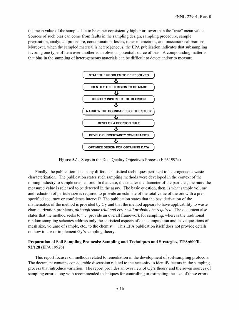
PNNL-22901, Rev. 0

A.16

the mean value of the sample data to be either consistently higher or lower than the “true” mean value. Sources of such bias can come from faults in the sampling design, sampling procedure, sample preparation, analytical procedure, contamination, losses, other interactions, and inaccurate calibrations. Moreover, when the sampled material is heterogeneous, the EPA publication indicates that subsampling favoring one type of item over another is an obvious potential source of bias. A compounding matter is that bias in the sampling of heterogeneous materials can be difficult to detect and/or to measure.

Figure A.1. Steps in the Data Quality Objectives Process (EPA1992a)

Finally, the publication lists many different statistical techniques pertinent to heterogeneous waste characterization. The publication states such sampling methods were developed in the context of the mining industry to sample crushed ore. In that case, the smaller the diameter of the particles, the more the measured value is released to be detected in the assay. The basic question, then, is what sample volume and reduction of particle size is required to provide an estimate of the total value of the ore with a pre-specified accuracy or confidence interval? The publication states that the best derivation of the mathematics of the method is provided by Gy and that the method appears to have applicability to waste characterization problems, although some trial and error will probably be required. The document also states that the method seeks to “… provide an overall framework for sampling, whereas the traditional random sampling schemes address only the statistical aspects of data computation and leave questions of mesh size, volume of sample, etc., to the chemist.” This EPA publication itself does not provide details on how to use or implement Gy’s sampling theory.

Preparation of Soil Sampling Protocols: Sampling and Techniques and Strategies, EPA/600/R-92/128 (EPA 1992b)

This report focuses on methods related to remediation in the development of soil-sampling protocols. The document contains considerable discussion related to the necessity to identify factors in the sampling process that introduce variation. The report provides an overview of Gy’s theory and the seven sources of sampling error, along with recommended techniques for controlling or estimating the size of these errors.

PNNL-22901, Rev. 0

A.17

In turn, these errors can be used as a guide in selecting the components of variance to be determined by a sampling effort.

The report indicates that laboratory methods have reached a point where analytical error contributes only a small portion of the total variance seen in results. It provides a specific example in which the results of a components-of-variance analysis performed on soils data indicated that 92 percent of the total variation came from the location of the sample, while only 8 percent was introduced after the sample was taken. Of this, less than 1 percent of the total variation was attributed to the analytical process.

The report outlines particulate sampling theory as developed by Gy. The sampling theory links the size of particles in the material of interest directly to the size of sample that is taken for evaluation, with the controlling particle size being the largest particle. Because the variability of particulate materials is based on the number of particles in the sample, samples with smaller particles will show lower variability in a given weight for analysis. Sometimes the process known as “communition” or reduction of particle size is conducted to achieve this, but as stated in the report, “… [it] may not be practical in environmental sampling because of safety, costs, and the handling requirements that are required to apply the theory.” For instance, the author states that “… much of the theory cannot be used in the case of volatile organic chemicals because of the grinding, mixing, and subsampling that is required to obtain a correct sample.” The publication provides considerable detail related to sources of variation and sampling errors as developed by Gy and defined further by Pitard. The report introduces the concept of sample correctness, which is a property of the material itself and the equipment used to extract the sample. In short, a sample is correct when all particles in a randomly chosen sampling unit have the same probability of being selected for inclusion in the sample. The report indicates that “grab samples” lack correctness and are therefore biased.

The EPA report also provides a discussion on how to determine the number of samples. As shown the following equation, approach used to estimate the initial sample size (or number) is exactly the same as that used in the WAC DQO.

/ 0.5

where:

n = number of samples Za = percentile of the standard normal distribution with Type I1 error = a Zb = percentile of the standard normal distribution with Type II2 error = b D = minimum relative detectable difference/CV CV = coefficient of variation

Regarding sample mass, the report also mentions Pitard’s procedure for determining the particle size-sample weight relationship that should be met to ensure that an unbiased sample of material is obtained for analysis. From this, an estimate of the variance of the fundamental error (FE) can be estimated (but not the FE itself). Again, the author indicates that parts of this sampling theory are applicable to soil

1 Type I error is defined in statistics as the incorrect rejection of a true null hypothesis (i.e., false positive). 2 Type II error is defined in statistics as the failure to reject a false null hypothesis (i.e., false negative).

PNNL-22901, Rev. 0

A.18

sampling, but some aspects of the theory cannot be carried out because of the requirement for grinding or pulverizing the sample to reduce the particle sizes to a size that maintains a desirable FE.

Correct Sampling Using the Theories of Pierre Gy (EPA 1999)

This short publication from the EPA highlights the importance of obtaining representative samples and ensuring their integrity throughout the analytical process. An overview of Gy’s theory, related to sampling correctness and representativeness as a critical component in the collection and handling of environmental samples, is provided. It states that the sampling theories of Gy are “… applicable to some sampling events at hazardous waste sites and to the successful subsampling of those samples at the analytical laboratory.” It offers that the practices suggested by Gy will result in samples that better represent the site and higher quality data for little or no added expense. Again, additional details related to the application of Gy’s sampling theory are provided in Section 3.

RCRA Waste Sampling Draft Technical Guidance: Planning, Implementation, and Assessment (EPA 2002)

This is an extensive guide that contains a significant amount of information related to a sampling and analysis program and its three main components of planning, implementation, and assessment. The guide has several sections pertaining to various components of a sampling program, with the most pertinent sections being optimizing the design for obtaining data and controlling variability and bias in sampling. The former section describes how to link the results of the DQO process with the development of a quality assurance project plan (QAPP). In short, one optimizes the sampling design to control sampling errors within acceptable limits and costs, while continuing to meet the sampling objectives. Results of the DQO are documented in a QAPP or similar planning document. Through this process, data requirements are translated into measurement performance specifications and quality assurance procedures. The latter section on controlling variability and bias indicates that random variability and bias (collectively known as “error”) in sampling account for a significant portion of the total error in the sampling and analysis process and that this “… far outweighs typical analytical error.” Thus, this section describes the sources of sampling error and provides some strategies for their minimization.

The guide also contains an appendix that identifies strategies for sampling heterogeneous wastes, which plays an important role in how to collect and handle samples and what type of sampling design to use. Another appendix is on a quantitative approach for controlling FE. This appendix includes an approach for determining the appropriate mass of a sample of particulate material based on information about the size and shape of the particles. The guide also discusses Gy’s theory and makes an important distinction between sampling error and statistical sampling designs. In particular, in the context of this guidance, Gy’s sampling theory is focused on minimizing error during the physical collection of samples. As such, this should not be confused with statistical sampling designs. In summary, both sampling theory and sampling design are critical elements in sampling. Gy’s sampling theory can facilitate collection of “correct” individual samples, while statistical sampling designs enable a statistical analyses and conclusions about the waste. To this end, the goal of applying the appropriate components of Gy’s theory to Hanford tank waste should further facilitate the effort to obtain such correct samples and then the statistical analysis as contained in the WAC DQO be used to make the acceptance decisions as written.

PNNL-22901, Rev. 0

A.19

Data Quality Assessment: Statistical Methods for Practitioners (EPA 2006a)

This guide describes the various statistical methods used in a Data Quality Assessment (DQA) while evaluating environmental data sets. Per the guide, “… DQA is the scientific and statistical evaluation of environmental data to determine if they meet the planning objectives of the project, and thus are of the right type, quality, and quantity to support their intended use.” The guide is intended to be a “tool-box” of techniques to assess the quality of data using a systematic methodology. The statistical techniques provided are demonstrated in the form of a series of steps to be taken and then are illustrated with an example. This is an all excellent reference for standard statistical practices and techniques pertinent to sampling analysis and the WAC DQO is consistent with this reference.

Guidance on Systematic Planning Using the Data Quality Objectives Process (EPA 2006b)

This guide presents the DQO process as EPA’s recommended planning process when environmental data are used to make a decision between two alternatives (in the case of Hanford tank waste, these alternatives are to accept the waste for transfer to the Waste Treatment Plant [WTP] or not). The DQO process is used to develop performance and acceptance criteria (or DQOs) that clarify study objectives, define the appropriate type of data, and specify tolerable levels of potential decision errors to be used as the basis for establishing the quality and quantity of data needed to support decisions. The DQO process is both flexible and iterative, and applies to both decision-making (e.g., compliance/non-compliance with a standard) and estimation (e.g., ascertaining the mean concentration level of a contaminant). Per the guide, the DQO process leads to efficient and effective expenditure of resources; consensus on the type, quality, and quantity of data needed to meet the project goal; and the full documentation of actions taken during the development of the project. Specific detailed steps to be followed in the DQO process are provided in the guide. The WAC DQO has followed these basic steps, and is consistent with the EPA’s guidance.

Guide for Industrial Waste Management; Chapter 2, Characterizing Waste, EPA530-R-03-001, (EPA 2012)

This EPA document provides overviews of different ways to characterize waste, including characterization through process knowledge and through leachate testing. Process knowledge refers to detailed information on the processes that generated the waste. Sometimes process knowledge can be used to partly or completely characterize waste for proper management. Process knowledge methods include the use of existing published or documented waste analysis data or studies conducted on wastes generated by processes similar to the process that generated the waste; waste analysis data obtained from other facilities in the same industry; and records of previously analyses performed at a facility.

Leachate and extraction testing is geared at estimating the leaching potential of constituents of concern to water sources (which is the context pertinent to this document). However, the document describes various methods that are in general applicable to this project report, including specification of a plan for sampling and analyzing the waste. In developing a sampling plan, accuracy is of primary concern, with the goal being to obtain an accurate estimate of the waste characteristics from measuring the sample characteristics. The controlling factor in determining the accuracy of the estimate is how representative the sample is where a “representative sample” is one that has the same properties and composition, and in the same proportions, as the population from which it was collected. Because most industrial wastes are not homogeneous, many different factors should be considered in obtaining samples.

PNNL-22901, Rev. 0

A.20

For instance, the samples should represent the average concentration and variability of the waste in time or over space. Furthermore, to ensure that results from waste sampling efforts are accurate, they must be unbiased and sufficiently precise. The document states that accuracy can be achieved by incorporating randomness into the sample selection process and by selecting an appropriate number of samples. The document also indicates that, for heterogeneous wastes, unbiased samples and appropriate precision can usually be achieved by simple random sampling. In this type of sampling, all units in the population (essentially all locations or points in all batches of waste from which a sample could be collected) are identified, and a suitable number of samples are randomly selected from the population. In the case of the Hanford tank waste, mixing and circulation of the waste for sample collection via the Isolok® sampler system is akin to simple random sampling in this case (assuming the tank is sufficiently mixed so that its contents are homogenous). Guidance for Obtaining Representative Laboratory Analytical Subsamples from Particulate Laboratory Samples (Gerlach and Nocerino 2003).

“An understanding of the primary sources of sampling uncertainty should prevent unwarranted claims and guide future studies toward correct sampling practices and more representative results.”

This EPA guide provides general guidelines for obtaining representative subsamples for the laboratory analysis of particulate materials using “correct” sampling practices and “correct” sampling devices. However, as pointed out in the document, this guidance is generally applicable to field sampling and is not limited to environmental subsamples. The document outlines issues involved with sampling particulate materials, principal causes of uncertainty introduced by sampling, suggested solutions to sampling problems, and a discussion of appropriate sample treatments.

The author discusses that any lot (e.g., a site, a section from a site, or a batch) of particulate material consists of particles with diverse characteristics with respect to size, shape, density, etc. This diversity coupled with lot-specific distribution of the analytes of interest, and uncertainties resulting from subsampling can lead to significant variability in results. The author states that by following “… correct sampling practices, all of the ‘controllable’ sampling biases and relative variances defined by the Gy sampling theory should be minimized such that a representative subsample can simply be defined by the relative variance of just one sampling error, the fundamental error (FE).” As will be discussed later, this FE is the minimum variance associated with the lot. The guide goes on to provide a thorough review of Gy’s theory. Table A.1 was extracted from the guide and summarizes the seven sampling errors associated with this theory, which will be applied and discussed in Section 3 of this report. For now we introduce the basic concept that the overall estimation error (OE) in obtained results is the difference between the analytical estimate of the analyte of interest and the true (usually unknown) value of that analyte. Further, this overall error can be decomposed into total sampling error (TE) and the analytical error (AE). That is:

OE = TE + AE

Furthermore, as will be discussed in the next section, TE can be decomposed as well into the seven sampling errors associated with Gy’s sampling theory as listed in Table A.1. That is:

TE = FE + GE + CE2 + CE3 + DE + EE + PE

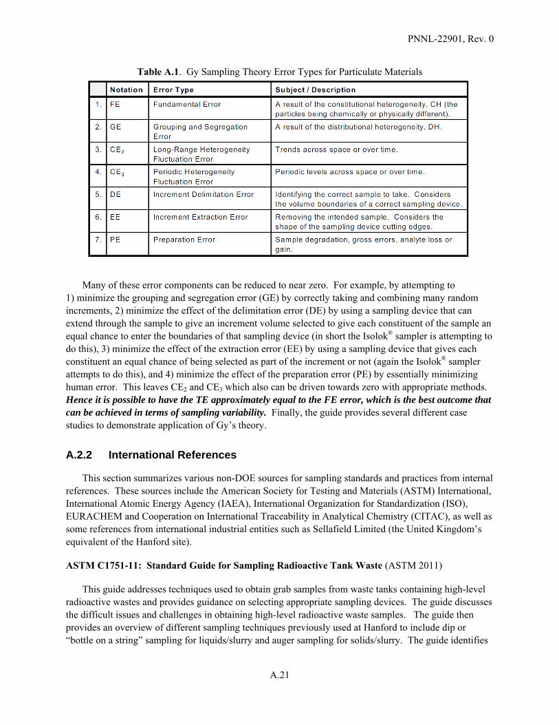
PNNL-22901, Rev. 0

A.21

Table A.1. Gy Sampling Theory Error Types for Particulate Materials

Many of these error components can be reduced to near zero. For example, by attempting to 1) minimize the grouping and segregation error (GE) by correctly taking and combining many random increments, 2) minimize the effect of the delimitation error (DE) by using a sampling device that can extend through the sample to give an increment volume selected to give each constituent of the sample an equal chance to enter the boundaries of that sampling device (in short the Isolok® sampler is attempting to do this), 3) minimize the effect of the extraction error (EE) by using a sampling device that gives each constituent an equal chance of being selected as part of the increment or not (again the Isolok® sampler attempts to do this), and 4) minimize the effect of the preparation error (PE) by essentially minimizing human error. This leaves CE2 and CE3 which also can be driven towards zero with appropriate methods. Hence it is possible to have the TE approximately equal to the FE error, which is the best outcome that can be achieved in terms of sampling variability. Finally, the guide provides several different case studies to demonstrate application of Gy’s theory.

A.2.2 International References

This section summarizes various non-DOE sources for sampling standards and practices from internal references. These sources include the American Society for Testing and Materials (ASTM) International, International Atomic Energy Agency (IAEA), International Organization for Standardization (ISO), EURACHEM and Cooperation on International Traceability in Analytical Chemistry (CITAC), as well as some references from international industrial entities such as Sellafield Limited (the United Kingdom’s equivalent of the Hanford site).

ASTM C1751-11: Standard Guide for Sampling Radioactive Tank Waste (ASTM 2011)

This guide addresses techniques used to obtain grab samples from waste tanks containing high-level radioactive wastes and provides guidance on selecting appropriate sampling devices. The guide discusses the difficult issues and challenges in obtaining high-level radioactive waste samples. The guide then provides an overview of different sampling techniques previously used at Hanford to include dip or “bottle on a string” sampling for liquids/slurry and auger sampling for solids/slurry. The guide identifies

PNNL-22901, Rev. 0

A.22

basic principles on sampling-plan design considerations to obtain accurate results from the samples taken. These principles, which are listed below, include guidance that are fairly consistent with the WAC DQO.

Identifying goals and confidence levels for decisions

Identifying locations for sampling and acknowledging that there could be limitations based on tank access

Identifying sources of variation through thorough interpretation of data/results. This last principle also highlights variations resulting from heterogeneity, which may be due to a combination of several factors (e.g., nature of the solids, mixing, selective settling in the tanks, etc.).

Finally, this guide hints that Gy’s sampling theory “… offers an approach to minimize error in sampling particulate solids.”

High-Level Waste Processing in the U.K. – Hard Won Experience that can Benefit U.S. Nuclear Cleanup Work (Dobson and Phillips 2006)

This conference paper reports that the constituents of the Sellafield (United Kingdom) high-level liquid waste and medium active liquid waste are similar to those in the high-level waste currently stored in alkaline form in carbon steel tanks at the Hanford and Savannah River sites. Figure A.2 shows a comparison of radioactive wastes at the respective sites. A key difference in waste management strategy in the United Kingdom is that wastes are processed and stored in the acidic form, thus requiring stainless steel equipment. The Sellafield high-level liquid waste evaporation and storage plant has a requirement to take representative samples for both process control and inventory purposes. The paper discusses the issues associated with suspended solids and the agitation systems used. A key point is that “… jets are angled so that the base area of the tank is completely swept, including the corner with the side wall.” It also is important to note that, similar to current testing at Hanford, at Sellafield full-scale testing using conservative simulants were used to demonstrate the functionality of the system. Another key point from this paper is that tanks are fitted with four air-lift recirculation (ALR) units which use compressed air to create an air-lift system within the tank. “This provides a very vigorous agitation of the tank contents and, in conjunction with the jet ballast tubes, completely homogenizes the tank contents. The jet ballasts operate continuously to keep solids in suspension, and the ALRs are used immediately prior to tank sampling operations.”

A key difference at Sellafield is that all of the storage tanks are fitted with liquid sampling systems that allow samples to be drawn from different points in the tanks. The paper goes on to describe key features and functions of the sampling system. This system has proven effective by taking and comparing samples from different points in the tank. Finally, the paper discusses fully automated systems that have been used extensively for the past 15 years, successfully taking and transporting samples of all level of activity direct from plant to laboratory, and how that these same autosamplers are to be installed in the Hanford WTP. Dobson and Phillips indicate that these autosamplers can be configured to work with a variety of sample delivery systems including proprietary sample collection systems such as the Isolok® sampler. In summary, this paper indicates some key differences and parallels between Sellafield and Hanford and support for the Isolok® sampling system. A key takeaway is the importance of representative sampling via sufficient tank mixing to obtain homogeneity. The paper does not provide any discussion on statistical methods or how to quantify uncertainty.

PNNL-22901, Rev. 0

A.23

Figure A.1. Total Curies of Waste Stored at Sellafield Site Compared with Hanford and Savannah River Sites (Dobson and Phillips 2006)

EURACHEM/CITAC Guide: Use of Uncertainty Information in Compliance Assessment, First Edition (Ellison and Williams 2007)

This guide focuses on accounting for measurement uncertainty in determining whether measurement results indicate compliance or non-compliance with a specification. The guide provides guidance on setting appropriate criteria for unambiguous decisions on compliance given results with associated uncertainty information. Figure A.3 was extracted the guide and provides a good overview and considerations for the WAQ DQO. In the figure, the solid line represents an action limit, and the bell-shaped curves represent typical probability distributions that might result from sampling along with their uncertainty intervals. In case (i) and (iv), decisions are easy; the feed is not accepted (i) and the feed is accepted (iv), respectively. However, in case (iii) for example, even though the sample mean is below the action limit, uncertainty, as indicated by the confidence interval extending beyond the action limits, indicates that either the waste in not accepted or perhaps it could be accepted based on an assessment of potential risks with making a wrong decision.

The guide goes on to discuss the concept of “decision rules” that give a prescription for the acceptance or rejection of a product (tank waste in this case) based on the measurement results, uncertainty, and specification limits, which also take into account the acceptable level of the probability of making a wrong decision. This prescription is consistent with the current WAQ DQO sampling design. The guide also presents the notion of a “Guard Band,” which can indicate the start of a rejection zone of waste acceptance that is based upon the action limit and a specified confidence level. In this case, a guard band is determined by multiplying a t-value with appropriate degrees of freedom and uncertainty measured by standard deviation and then subtracting this from the action limit. This approach is essentially equivalent to a confidence interval approach. However, the method can provide an a priori

PNNL-22901, Rev. 0

A.24

expectation on the required mean level of the constituent being measured for a given sample size and assumed uncertainty.

Figure A.2. Assessment of Compliance with an Upper Limit (Action Limit) (Ellison and Williams 2007)

For instance, for acceptance of a particular action limit based on the sample size, n (e.g., n = 3), assumed variability (e.g., sampling relative standard deviation [RSD] = 10 percent), and desired confidence level (e.g., 90 percent). In this case the guard band would indicate that the mean of the three samples needs to be at least 20 percent less than the action limit. As variability increases (say RSD = 20 percent), the mean of the three samples needs to be at least 38 percent less than the action limit. Conversely, if variability were reduced (say to RSD = 4 percent), then the mean of the three samples would only need to be about 8 percent less than the action limit. Hence, the importance of sampling variability and efforts to minimize it can be seen in these simple calculations.

EURACHEM/CITAC Guide CG4: Quantifying Uncertainty in Analytical Measurement, Third Edition (Ellison and Williams 2012)

“Whenever decisions are based on analytical results, it is important to have some indication of the quality of the results, that is, the extent to which they can be relied on for the purpose in hand.”

This EURACHEM/CITAC guide introduces the concept of uncertainty and the distinction between uncertainty and error. The guide defines uncertainty as “… a parameter associated with the result of a measurement, that characterizes the dispersion of the values that could reasonably be attributed to the measurand” and error as “… the difference between an individual result and the true value of the measurand.” It also is noted that error cannot be known exactly because the true value is unknown. The guide also provides a description of the steps involved in the evaluation of uncertainty. Although the application is geared at uncertainty associated with chemical measurements, the process is applicable to characterizing uncertainty in general. Thus, the guide provides a good overview with respect to uncertainty considerations with respect to Hanford waste tanks. In short, the evaluation of uncertainty requires one to first consider all possible sources of uncertainty. The editors indicate that a study will quickly identify the most significant sources of uncertainty and how the value obtained for the combined uncertainty is almost entirely controlled by the major contributions. This implies that a good estimate of uncertainty can be made by concentrating effort on the sources that make the largest contributions.

PNNL-22901, Rev. 0

A.25

Moreover, potential sources of uncertainty can be further investigated and methods employed to reduce the uncertainty to an acceptable level where possible.

For a particular measurement result, total uncertainty or combined standard uncertainty is an “…estimated standard deviation equal to the positive square root of the total variance obtained by combining all the uncertainty components.” The editors provide the following summary of steps that should be performed to estimate of the uncertainty associated with a measurement result. These steps are essentially the steps followed in the WAC DQO for estimating sample sizes for the various action limits.

Step 1. Specify Measurand ‒ Write down a clear statement of what is being measured.

Step 2. Identify Uncertainty Sources ‒ List the possible sources of uncertainty.

Step 3. Quantify Uncertainty Components ‒ Estimate the size of the uncertainty component associated with each potential source of uncertainty identified.

Step 4. Calculate Combined Uncertainty ‒ Combine the quantified contributions to overall uncertainty in Step 3, expressed as standard deviations, to give a combined standard uncertainty.

A very important point made by the editors is to recognize that not all of the components will make a significant contribution to the combined uncertainty. In fact, they indicate that, in practice, it is likely that only a small number of components are significant. They suggest that unless there are a large number of them, those components that are less than one-third of the largest do not need to be evaluated in detail. Accordingly, a preliminary estimate of the contribution of each component or combination of components to the uncertainty should be made and those that are not significant be eliminated. Just to consider an example, if sampling uncertainty is RSD = 10 percent and analytic uncertainty is RSD = 4 percent, the combined uncertainty would be RSD = 10.8 percent. In this case then, the analytic uncertainty is contributing only a small contribution to the overall uncertainty.

Finally, as shown and exemplified in this guide, a cause-and-effect diagram can be used as a way of listing sources of uncertainty sources, showing how they relate to each other, and indicating their influence on the overall uncertainty of the result. The editors state that a cause-and-effect diagram also helps to avoid double counting of sources. Thus, a cause-and-effect diagram might be a possible tool for application to Hanford waste tank characterization.

International Target Values 2000 for Measurement Uncertainties in Safeguarding Nuclear Materials (Aigner et al. 2002)

This bulletin published by the European Safeguards Research and Development Association contains tables on International Target Values that are uncertainties to be considered in judging the reliability of analytical techniques applied to industrial nuclear and fissile material, which are subject to safeguards verification. The tabulated values represent estimates of the “state of the practice” that should be achievable under routine measurement conditions. The specific application of these Internal Target Values for Hanford waste characterization in uncertain, but the important aspect of this bulletin is the recognition of sound statistical practices as well as the need to characterize uncertainty. In that regard, the bulletin outlines appropriate statistical terminology to include basic terms and selected sources and classes of error that resemble the errors articulated in Gy’s sampling theory. The bulletin also

PNNL-22901, Rev. 0

A.26

summarizes descriptors such as precision and accuracy that are similar to the previously discussed definitions of these terms. Finally, the bulletin lists terms that are specific to safeguards. Among these terms is “risk.” Risk is a synonym for the probability of reaching the incorrect conclusion in hypothesis testing, which is similar to the definition of risk used in the WAC DQO.

Strategy and Methodology for Radioactive Waste Characterization (IAEA 2007)

This IAEA publication reviews the requirements for and development of a waste characterization program strategy, quality assurance, and quality control activities at different waste generators. The document also reviews the important factors to be considered in a waste-characterization program, including accuracy and uncertainties, scaling factors, and measurement methods. It also provides a discussion on the most commonly used characterization methods and techniques, as well as an example calculation of uncertainties when dealing with samples assumed to be representative.

The publication indicates that there are multiple sources of uncertainty and their identification, definition and quantification is one of the main tasks in setting up a characterization process. Similar to the other reviews examined thus far, it identifies the most relevant sources of uncertainty as 1) incomplete definition of the sample that will be analyzed, 2) deviation or bias in the reading of an instrument, 3) instrument resolution, 3) value assigned to the reference data or parameters, 4) representativeness of the sample measured, and 5) environmental conditions. The guide also discusses random and systematic errors and how they can be evaluated. It states that a definition of systematic error is the bias or the difference between the real value and the one obtained in the measurement. Finally, the paper introduces the notion of an uncertainty budget that essentially is a breakdown of uncertainty into its various components. The publication does not have any direct references to Gy’s sampling theory nor its use in waste characterization.

Copper, Lead, Zinc and Nickel Concentrates ‒ Sampling Procedures for Determination of Metal and Moisture C (ISO 2005)

Although geared at basic methods for sampling copper, lead, zinc and nickel concentrates from moving streams and stationary lots, this international standard contains pertinent general information related to obtaining samples for chemical analysis. In this case, the common sample must be sufficiently representative (unbiased and sufficiently precise). The standard indicates that large agglomerates (>10 mm) present in the primary sample should be crushed prior to further sample processing. Although the focus is on solids, the document states that sampling from moving streams is the preferred method. This is because taking samples from stationary lots minimizes some of the systematic sampling errors. The overall “… general aim of a sampling scheme is to provide one or several test portions, sufficiently representative of a lot, for determination of the quality characteristics of the lot.” As seen before, the standard provides that the total variance of the final result is composed of the variance of sampling (including sample processing) plus the variance of chemical analysis. This standard does reference and apply Gy’s sampling theory.

PNNL-22901, Rev. 0

A.27

EURCHEM/CITAC Guide: Measurement Uncertainty Arising from Sampling. A Guide to Methods and Approaches (Ramsey and Ellison 2007)

“It has become increasingly apparent that sampling is often the more important contribution to uncertainty and requires equally careful management and control.”

This guide provides a thorough review of methods that can be used to assess uncertainty in measurements that arise from sampling. It initially highlights the need to sample for the measurement of a property of interest as it is usually impossible to analyze the entire sample population (e.g., entire Hanford waste tank contents). If the objective of the measurement is to estimate the value of the analyte concentration in a waste tank example, then the uncertainty associated with the sampling process contributes to the uncertainty associated with the reported result. Hence, uncertainty arising from the sampling process itself must therefore be evaluated. Accordingly, this guide aims to describe various methods that can be used to estimate the uncertainty of measurement, and those particularly arising from the processes of sampling as well as the physical preparation of samples to be analyzed. The guide states that it takes a “holistic view” of the entire measurement process, to include the analytical process, in the case where the measurand is defined in terms of the value of the analyte concentration in the sampling target, rather than in just the sample delivered to the laboratory.

The guide begins by explaining “… the importance of knowing the total uncertainty in a measurement for making reliable interpretation of measurements, and judging their fitness for purpose.” The guide highlights the two main approaches for estimating sampling uncertainty: 1) the empirical approach, which “… uses repeated sampling and analysis under various conditions to quantify the effects caused by factors such as the heterogeneity of the analyte in the sampling target and variations in the application of one or more sampling protocols to quantify uncertainty (and usually some of its component parts),” and 2) the modeling approach, which “… uses a predefined model that identifies each of the component parts of the uncertainty, makes estimates of each component, and sums them to make an overall estimate.” The guide indicates that models from sampling theory can be used in this approach to estimate some of the uncertainty components based on knowledge of the characteristics of particulate constituents. In this case, as with many of the other documents previously reviewed, this guide also contains coverage on Gy’s sampling theory and the seven sources of sampling errors.

Sellafield Sampling Techniques – Draft Technical Report (CCN: 255475, WTP 2013, Sellafield 2013)

This guide specifically focuses on nuclear waste sampling and emphasizes that identifying the required analysis or measurement is as important as the sampling itself. The guide also stresses consideration of how the characterization requirements are established and provides guidance on establishing sample analysis programs and that these should include:

Determine what needs to be known

How accurately it needs to be known

How it will be determined

What the associated uncertainties are

Establish good records

PNNL-22901, Rev. 0

A.28

Minimize the number of samples required to resolve an issue

Reduce the size of the sample required

Provide data up front that can allow identification of the correct sampler and activity assessment of samples from unknown wastes.

Several of these considerations are actually already included in the WAC DQO. The guide also provides insights on a “robust approach to sampling” that, for now, is essentially covered in the error tolerance and sampling design sections of the WAC DQO.

The guide also reviews various samplers that have previously been used at Sellafield and in the United States. None of the samplers listed in this regard closely resemble the Isolok® sampler, although the reports does provide mention of generic syringe type samplers without detailed information.

The guide does provide some information related to sample size. In particular, the guide states that the optimum sample size should be large enough so that the mean value obtained from this quantity does not differ significantly from the mean value for the lot from which the quantity was taken. Moreover, a sample should be large enough to permit three replicate analyses. The guide discusses that the sample size is dependent upon the risk of having a result or mean value differing from the mean value of the lot characteristic by a specified percentage (akin to the WAC DQO error tolerance section). Moreover, without specifically referencing Gy’s sampling theory, the guide indicates that “… for sludges, the sample size should be governed by the largest size within the distribution (of interest) because the smaller particle sizes will have a bigger number of particles per gram than the largest size range.”

A.2.3 Other Non-DOE References

Additional non-DOE references outside of EPA and international sources are reviewed below.

Statistical Methods for Nuclear Material Management (Bowen and Bennett 1988)

This source is a U.S. Nuclear Regulatory Commission sponsored report on statistical methods used in nuclear material management. The text provides a very thorough review and detailed mathematical methods on applicable statistical methods. The text also discusses unique problems encountered in nuclear material management that go beyond general statistical methods, to include multiplicity of error sources in a material balance and estimation of the variance components associated with each error source. The text provides significant coverage on hypothesis testing, to include sample size estimation that is consistent with the WAC DQO methodology. It also provides a detailed discussion on sequential tests and how this method can result in smaller sample sizes needed to obtain a decision than with other methods and provides a detailed illustration. This approach is closely related to the current sampling plan in the WAC DQO.

In regard to sampling, this report also discusses the importance of representative samples which depends on both the homogeneity of the material being sampled and the sampling method. It discusses that the most effective way to avoid both random error and bias in sampling is to blend the material to a homogenous state before sampling, which is the current plan with respect to the Hanford waste tanks.

PNNL-22901, Rev. 0

A.29

The text also discusses minimizing the effects of heterogeneity by drawing many subsamples from the batch and compositing them for analysis.

Incremental Sampling Methodology (ITRC 2012)

“The fundamental purpose of sampling is to obtain data that will support decision-making about an area or volume of material that is impractical or impossible to analyze in its entirety.”

This document focuses on the application of incremental sampling methodology (ISM) as a structured composite sampling and processing protocol. The document states that ISM can reduce data variability and provide “… a reasonably unbiased estimate of mean contaminant concentrations in a volume of soil targeted for sampling.” Soil sampling is the focus of the document, but general methods and principles are still applicable to Hanford tank waste sampling. In short, ISM provides a way to obtain representative samples of specific soil volumes defined as “… decision units (DUs) by collecting numerous increments of soil (typically 30 to 100 increments) that are combined, processed, and subsampled according to specific protocols.” The authors state that ISM provides reliable, reproducible sampling results and leads to better, more defensible decisions than have typically been achieved with many traditional sampling approaches. Such improvements result from the inherent attributes of ISM and the details of its implementation, including a clearer connection between sampling objectives and sampling approach. ISM works to address and overcome the sampling errors associated with soil sampling, integrates attention to detail in planning and field work, and requires attention to quality assurance/quality control measures throughout the sampling effort and not just in the laboratory.

This document also contains a significant discussion on Gy’s sampling theory and the seven basic sampling errors. Again, discussions applying Gy’s sampling theory are withheld until Section 3. For now, the document states that the use of Gy’s incremental sampling approach to collect samples from environmental bulk materials (e.g., soils, sediments, liquids, etc.) is a relatively new concept in contaminated site investigation. The authors provide that important concepts underlying Gy’s sampling principles (and ISM) are reflected by addressing the following questions:

What are the differences between bulk material sampling and traditional random sampling of discrete items (e.g., individuals in a room, discrete data sets consisting of 100 distinct points, or even 10,000 distinct points)?

How can Gy’s sampling principles be used to collect representative (unbiased) samples from environmental bulk materials?

Which heterogeneities are sources of sampling error, identified by Gy’s sampling theory, are addressed by ISM?

What is the difference between the heterogeneities present in the bulk material to be sampled and the variability in the analytical results obtained by chemical analysis of collected samples?

Additional key points from this document that directly relate to the WAC DQO are discussed below. The document presents various different decision mechanisms, one of which parallels the WAC DQO exactly; that is, comparison of the 95 percent upper control limit (UCL) on the mean of replicate data from the decision unit (in this case the decision unit would be a specific Hanford waste tank) to the action

PNNL-22901, Rev. 0

A.30

level (or action limit). Under this decision mechanism, the guide states that, when the true mean is well above or below an action level, even a small number of discrete samples usually results in a correct decision (this point was made earlier). At the same time, the document recognizes that the likelihood of underestimating the mean from any sampling method (i.e., discrete, composite, or ISM) increases as the degree of heterogeneity increases. This also argues to smaller particle size if possible. Traditionally, with discrete samples, the concern for underestimating the mean has been addressed by specifying an acceptable level of uncertainty (often 5 percent) and a method for calculating a conservative estimate of the mean (e.g., a 95 percent UCL). This is the approach in the WAC DQO. One last point made in this document is that a low RSD is not an indication that the mean is accurate or that the 95 percent UCL exceeds the population mean unless the distribution can be reasonably assumed to be relatively homogeneous. Thus, once again the importance of a homogenous tank waste for sampling is paramount. On the topic of heterogeneity, the document provides Figure A.4, which summarizes how heterogeneity can lead to decision errors.

Figure A.3. Heterogeneous Nature of Contaminants in Soils may lead to Decision Errors (ITRC 2012)

Multi-Agency Radiological Laboratory Analytical Protocols Manual, Volume III: Chapters 18-20 and Appendix G (MARLAP 2004)

“The claim is often made that field sampling uncertainties are so large that they dwarf laboratory measurement uncertainties. Although the claim may be true in some cases, MARLAP rejects this argument as an excuse for failing to perform a full evaluation of the measurement uncertainty. A realistic estimate of the measurement uncertainty is one of the most useful quality indicators for a result.”

This manual discussed the evaluation and reporting of measurement uncertainty so it is only lightly summarized here as the focus of this project is sampling uncertainty. Key points included that laboratory measurements always involve uncertainty, which must be considered when analytical results are used as part of a basis for making decisions (which they are as documented in the WAC DQO as analytical error). Thus, one purpose of this manual is to provide an understanding of the causes of measurement uncertainty and of the meaning of uncertainty statements in laboratory reports. The manual also described procedures which laboratory personnel use to estimate uncertainties.

Even though the manual focuses on laboratory measurement and uncertainty, key aspects associated with sampling are identified, such as uncertainty caused by the subsampling of heterogeneous solid matter. The document stated that even though it may be “… difficult to estimate, it should not be ignored, since it may be relatively large and in some cases may even dominate all other components.” It also indicated that one may use previous experience with similar materials to evaluate the uncertainty.

PNNL-22901, Rev. 0

A.31

Finally, the manual provided a means of estimating uncertainty associated with subsampling, which depends on the maximum particle diameter, the mass of the sample, and the mass of the subsample and provides an equation for the standard uncertainty based on these parameters which is based on Gy’s theory.

Geostatistical Error Management: Quantifying Uncertainty for Environmental Sampling and Mapping (Meyers 1997)

“Heterogeneities are not errors in themselves; rather, they are structural properties that enable sampling errors to arise.”

This reference is a textbook that contains mathematical relationships and quantitative tools for sampling in environmental applications. Its overarching framework is known as geostatistical error management (GEM). A full review is beyond the scope of this project report, but as an overview, GEM is intended to integrate DQOs, sampling theory and practice, and geostatistical appraisal to “create an entirely new set of tools” to help to more accurately assess needed resources for collecting data, analyzing sampling sources of error, and quantifying results. The author outlines each of the three GEM components in more detail where the DQO process follows the EPA guidelines, sampling theory and practice follows Gy’s theory where the objective is to “obtain sample data that reflect as accurately as possible the true in situ contaminant concentrations,” and geostatistical appraisal is focused on analyzing (via various statistical tools such as variogram and kriging), and mapping results. Elements related to Gy’s sampling theory from this text will be explored further in Section 3. In regard to geostatistical appraisal, because the Hanford waste tanks are assumed to be thoroughly mixed and access to various points within the tank is limited, mapping of concentrations within the tanks is restricted. Also, a variogram is usually focused on analyzing the variance of the difference between two variables at two locations separated in space, thus it has a spatial orientation. Hence, applicability in regard to the Hanford waste tanks is limited. However, a variogram also can be used to assess the “stationarity” (a stationary time series is one whose statistical properties such as the mean and variance are all constant over time) of a time series, which may have an application for the samples that are collected from the Isolok® sampler over some time stratum. This will also be explored further in Section 3.

Pierre Gy's Sampling Theory and Sampling Practice: Heterogeneity, Sampling Correctness, and Statistical Process Control, Second Edition (Pitard 1993)

This text by Pitard is considered one of the classics in regard to presenting Gy’s sampling theory. The text provides an in-depth presentation on key terminology, all of the mathematical expressions needed to assess sampling errors, and example applications and quantitative results. Of course the text covers all of the Gy’s sampling errors and again a more detailed discussion on these is held until Section 3. The heart of the text is that sampling is “… an error-generating process directly related to the amount of heterogeneity in the lot.” The text would characterize the stream that will be sampled via the Isolok® sampler as a one-dimensional lot and presents a methodology to characterize the heterogeneity of such one-dimensional lot via variography (or a semi-variogram that the author states is most often called the variogram). In this context, Pitard assumes a moving one-dimensional stream of particulate material equipped with a sampling station (i.e., the Isolok® sampler in the case of Hanford) that can select correctly delimited and extracted increments at any interval of time. The text then goes on to develop total heterogeneity supported by such a one-dimensional lot. This development and potential application will be explored further in Section 3. An important point made in the text is that, regardless of how well a

PNNL-22901, Rev. 0

A.32

tank is mixed or “homogenized,” there will still always be heterogeneity (i.e., constitution heterogeneity that is associated with particles themselves being different from one another).

Measuring and Calculating Sampling Uncertainty (ALP 2007a)

This procedure provides guidance on estimating and calculating sampling uncertainty for representative samples from analytical measurements and related knowledge of the sampling equipment and protocols. It also provides guidance for assessing homogeneity in bulk materials for several types of samples. This procedure is intended to demonstrate uncertainty calculations where replicate measurements are available on at least duplicate samples. The document provides a summary of key terms and definitions such as material homogeneity, representative sampling, sampling uncertainty, and sampling and measurement errors. In regard to homogeneity and inhomogeneity (or heterogeneity), the guidance suggests that, for resulting protocols, there is a minimum agitation time for bulk liquids. Representative sampling is a process that by its design and/or nature provides samples that are representative of the stream or bulk material from which the samples were taken. Representative sampling also refers to the procedures and protocols that ensure a set of samples represents the conditions of a system, a location, or an individual at the specific time when the samples are taken. Sampling uncertainty is defined as the combined (propagated) systematic and random uncertainties associated with the sample collection process. This uncertainty often includes the variation in the samples (both random and systematic) generated by actions that are taken to prepare a system for sampling, which is one of the sampling errors identified by Gy’s sampling theory. Finally, sampling error and measurement error are typically used to refer to generating and delivering non-representative samples as well as reporting erroneous results.

Measurement Control Programs – General Requirements (ALP 2007b)

This procedure provides guidance on estimating the uncertainty for analytical measurement methods. It indicates that all measurements have uncertainty associated with them and that the result of a measurement is only an approximation of the value of the quantity being measured. Accordingly the result is complete only when accompanied by a statement of its uncertainty. This document also includes key terms and definitions. The guidance provides two classifications of uncertainty: Type A components, which are components of uncertainty evaluated by statistical methods (e.g., estimated standard deviation) and Type B components, which are usually based on expert judgment using relevant information available. In the latter case, uncertainty components are still converted to a quantified measure. Even though this guidance is geared at measurement uncertainty, Figure A.5 was reproduced from this procedure and is generally applicable to sampling uncertainty with one of the key pieces being Step 2, “Identify Uncertainty Sources.” The procedure states that one should realize that not all of the components will make a significant contribution to the combined uncertainty, but rather it is likely that only a small number will. It provides that components that are less than one-fourth the largest uncertainty component need not be evaluated in detail. However, a key part is to document these uncertainty components as having been evaluated, but eliminated for the final uncertainty calculation. The procedure also suggests that uncertainty contributions based on experimental studies specific to individual parameters be used.

PNNL-22901, Rev. 0

A.33

Measuring and Calculating Method Uncertainty (ALP 2007c)

This procedure contains general elements for an effective measurement control program for any measurement process implemented to provide accurate and reliable analytical services. As this is a general guide, specific steps are not provided in detail, but some key points found in the document are highlighted as follows:

The validity of samples must be assured through representative sampling techniques.

These techniques should be developed from sample evaluation for homogeneity.

Homogenous samples, such as liquids, may be subsampled without introducing a systematic error by taking aliquots.

Nonhomogeneous samples may require special techniques and studies to determine the techniques required for a representative subsample. 

A Primer for Sampling Solids, Liquids, and Gases: Based on the Seven Sampling Errors of Pierre Gy (Smith 2001)

“Without a doubt, all the materials we sample are heterogeneous, whether they are solids, liquids, gases or a combination.”

This text focuses on Gy’s sampling theory, but via a condensed discussion that focuses on essential aspects of the theory. The author starts with a discussion on the goal of good sampling, that is “… to follow a sampling protocol that produces a sample whose chemical or physical measurements of interest are 1) representative of the entire lot and 2) as consistent as possible, theoretically, with other samples that would be obtained if the entire sampling protocol could be repeated.” The author indicates that obtaining representative samples requires using physical sampling techniques that reduce the bias as much as possible and obtaining consistent samples means reducing sample-to-sample variation. The author also highlights some good sampling practices, which are paraphrased below:

Mix the material before sampling.

Take several increments and composite them to form the sample.

Collect the sample in an inert container.

Sample frequently enough to allow for identification of process cycles.

The text goes on to indicate that these are only some good sample practices and that Gy addresses these and other sampling questions through a structured approach. This approach will be covered further in Section 3. For now, we note that Smith takes Gy’s seven sampling errors and groups them into the three broad categories of 1) material variation, 2) tools and techniques, and 3) process variation. The author’s overview of heterogeneity and discussion on the presence of heterogeneity is why physical samples differ and why they generate variation. As mentioned earlier, there are two types of heterogeneity associated with sampling errors: 1) constitution heterogeneity and 2) distribution

PNNL-22901, Rev. 0

A.34

heterogeneity. Finally, the author states that from “Gy’s perspective, ‘Heterogeneity is seen as the sole source of all sampling errors’.”

The Fundamental Relationship between Sample Mass and Sampling Variance in Real Geological Samples and Corresponding Statistical Models (Stanley 2007)

This manuscript recaps that efforts to reduce sampling error have relied on the belief that larger samples exhibit less sampling error, which is consistent with Gy’s theory. The author provides a review of the theoretical justifications for this belief along with empirical tests of geological materials that to show an inverse relationship between sample size and sampling variance. Using a first principles approach, the paper provides proof of this relationship in all geological materials. Proof that sampling variance is inversely proportional to sample mass in real geological materials demonstrates that the foregoing assumption is correct. This result indicates that scientists can now confidently perform mass-standardization corrections to sampling variance data to allow calculation of average sampling variance from samples with different masses. Furthermore, geoscientists can now confidently compare mass-standardized sampling variances acquired using different sampling methods to assess whether real differences exist in the resulting sampling variances (i.e., can estimate the variance and correct for it by the actual mass of the sample used). In summary, this paper lends support to the idea that larger samples masses are better for reducing the effects of heterogeneity.

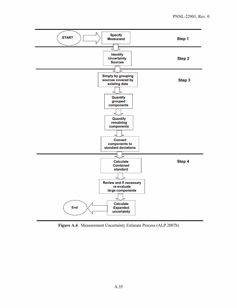
PNNL-22901, Rev. 0

A.35

Figure A.4. Measurement Uncertainty Estimate Process (ALP 2007b)

PNNL-22901, Rev. 0

Appendix B

Visual Sample Plan

 

PNNL-22901, Rev. 0

B.1

Appendix B

Visual Sample Plan

B.1 VSP Overview

The Visual Sample Plan (VSP) is a software tool that supports the development of a defensible sampling plan based on statistical sampling theory and the statistical analysis of sample results to support confident decision-making (PNNL 2011). VSP couples site, building, and sample location visualization capabilities with optimal sampling design and statistical analysis strategies. VSP is especially adept at answering the following questions:

How many samples do I need?

Where should I take samples?

What decisions do my data support?

How confident am I in those decisions?

B.2 VSP Applications

Developed with support from the U.S. Department of Energy, U.S. Environmental Protection Agency, U.S. Department of Defense, the U.S. Department of Homeland Security, the Centers for Disease Control and Prevention, and the United Kingdom, VSP has more than 5000 users. VSP has many sampling design and statistical analysis modules focused on soils, sediments, surface water, streams, groundwater, buildings, and unexploded ordnance sites. Many statistical sampling designs are available including random, systematic, sequential, adaptive cluster, collaborative, stratified, transect, multi-increment, combined judgment/probabilistic, and rank set sampling. VSP is being recommended by many regulators for defensible sampling design and statistical analysis. VSP is currently focused on design and analysis for the following applications:

Environmental characterization and remediation

Environmental monitoring and stewardship

Response and recovery of chemical/biological/radiation terrorist event

Footprint reduction and remediation of unexploded ordnance sites

Sampling of soils, buildings, groundwater, sediment, surface water, subsurface layers.

PNNL-22901, Rev. 0

B.2

The underlying methodology employs statistically defensible approaches and has strong Data Quality Objectives (DQO) Process underpinnings. The objective is to ensure that the right type, quality, and quantity of data are gathered to support confident decisions. VSP allows real-time evaluation of the tradeoffs between increased confidence in decisions and costs or number of samples required. VSP answers the questions of how many samples are required and where samples should be obtained. Designed for the non-statistician, VSP is organized around the possible data uses. Before developing a data-gathering plan, each user must determine what they will do with the data to support their decision-making process.

VSP currently supports the following sampling goals or objectives:

Estimate or compare averages

Compare individual sample results against some limit

Do transect or anomaly sampling/analysis for unexploded ordnance sites

Evaluate trends over time

Develop a geospatial contaminant concentration map

Evaluate well placement redundancies or inadequacies

Explore correlation between multiple analytes

Estimate or compare proportions

Assess whether the boundary around an area is contaminant free

Develop a targeted, purely judgmental sampling scheme

Sampling items.

B.3 VSP Demonstration

VSP is available for download from the following site: http://vsp.pnnl.gov/. Once downloaded and installed, the user will see the following (Figure B.1) when first launching the tool. As shown in Figure B.2, From here, the user can select “Sampling Goals” from the menu and the dropdown selection “Compare Average to Fixed Threshold …” to obtain sample size information. Figures B.3 – B.5 then demonstrate its use for notional settings associated with the Waste Acceptance Criteria (WAC) DQO action limit for “Pu to Metals Loading Ratio” (which has action limit of < 6.2 g/kg). The first setup in this case assumes normally distributed data and ordinary sampling. It is also initially assumed the waste is unacceptable until proven otherwise. For this analyte, the confidence level in the WAC DQO is 95 percent and also 95 percent power (or equivalently a 5 percent chance of incorrectly accepting the null). It is then assumed the true mean is 2.0 units below the action limit. Lastly, using the analytical RSD of 3.3 percent and sampling RSD of 10 percent as provided in Figure 7-10, Sample Size Graph – Pu to Metals Ratio in Solids, of the WAC DQO (which results in an estimated standard deviation due to sampling and analytical variability of 0.653 units based on the conservative approach of using the action

PNNL-22901, Rev. 0

B.3

limit as the mean), the estimated sample size returned by VSP is 3. In Figure B.4, the setup is the same except the true mean is 4.0 units below the action limit. In this case, the estimated sample size returned by VSP is 2. Lastly, In Figure B.5, the setup is also the same except the true mean is only 1.0 units below the action limit. In this case, the estimated sample size returned by VSP is 6. Thus, this simple demonstration provides insights into 1) the ease of use of VSP and 2) implications of different inputs associated with different waste decision parameters and results.

Figure B.1. Visual Sample Plan Start Page

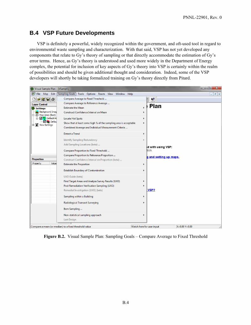
PNNL-22901, Rev. 0

B.4

B.4 VSP Future Developments

VSP is definitely a powerful, widely recognized within the government, and oft-used tool in regard to environmental waste sampling and characterization. With that said, VSP has not yet developed any components that relate to Gy’s theory of sampling or that directly accommodate the estimation of Gy’s error terms. Hence, as Gy’s theory is understood and used more widely in the Department of Energy complex, the potential for inclusion of key aspects of Gy’s theory into VSP is certainly within the realm of possibilities and should be given additional thought and consideration. Indeed, some of the VSP developers will shortly be taking formalized training on Gy’s theory directly from Pitard.

Figure B.2. Visual Sample Plan: Sampling Goals – Compare Average to Fixed Threshold

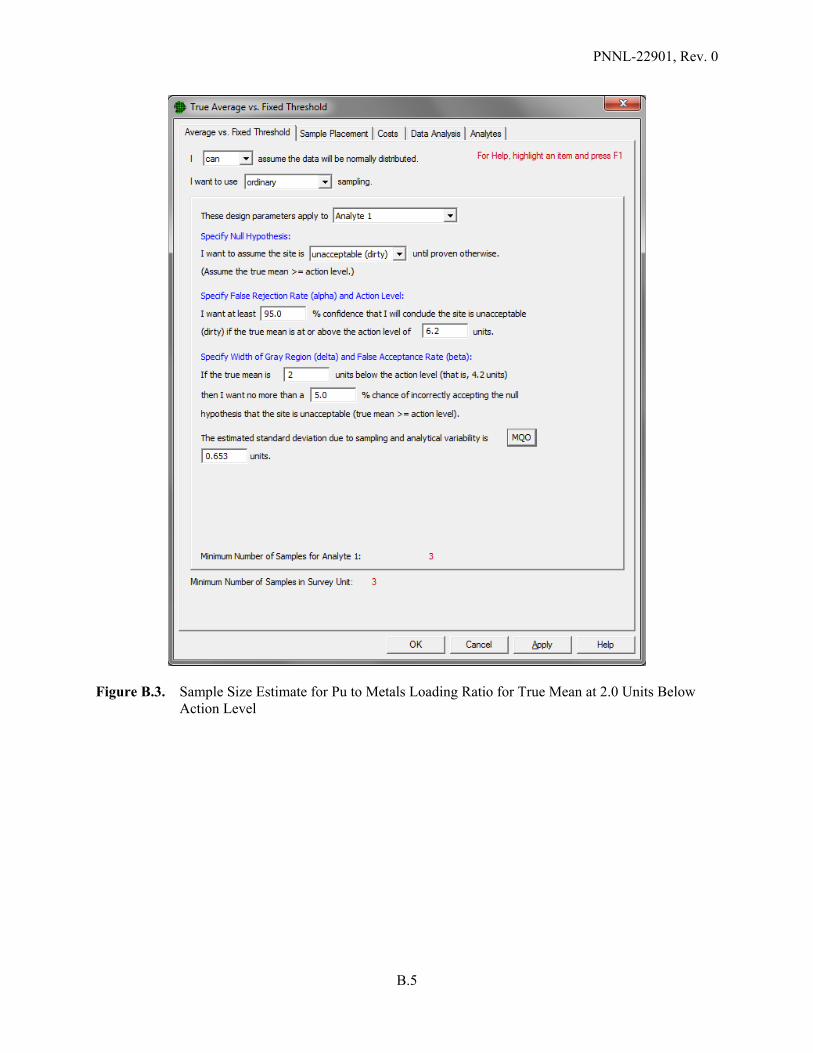
PNNL-22901, Rev. 0

B.5

Figure B.3. Sample Size Estimate for Pu to Metals Loading Ratio for True Mean at 2.0 Units Below

Action Level

PNNL-22901, Rev. 0

B.6

Figure B.4. Sample Size Estimate for Pu to Metals Loading Ratio for True Mean at 4.0 Units Below Action Level

PNNL-22901, Rev. 0

B.7

Figure B.5. Sample Size Estimate for Pu to Metals Loading Ratio for True Mean at 1.0 Unit Below

Action Level

PNNL-22901, Rev. 0 EMSP-RPT-016

Distribution*

No. of No. of Copies Copies

Dist. 1

2 DOE Headquarters Office of Environmental Management NP Machara SP Schneider 6 DOE Office of River Protection JA Diediker TW Fletcher BJ Harp CC Harrington P Logan SH Pfaff 3 Washington River Protection Solutions ST Arm MG Thien LE Thompson 1 Savannah River National Laboratory CC Herman 1 Bechtel National, Inc. AV Arakali 1 URS Corporation JR Markillie *All distribution will be made electronically.

5 Pacific Northwest National Laboratory PR Bredt RT Brigantic MS Fountain RA Peterson S Schlahta