STATISTICAL TUNING OF COST 231 HATA MODEL IN DEPLOYED

* Corresponding author, tel: +234 – 817 – 206 – 9243

STATISTICAL TUNING OF COST 231 HATA MODEL IN DEPLOYED

1800MHZ GSM NETWORKS FOR A RURAL ENVIRONMENT

E. L. Omoze1,* and F. O. Edeko2 1, 2, DEPARTMENT OF ELECTRICAL AND ELECTRONIC ENGINEERING, UNIVERSITY OF BENIN, BENIN CITY, EDO

STATE, NIGERIA

Email addresses: 1 [email protected], 2 [email protected]

ABSTRACT

Radio propagation planning requires the use of propagation models in planning cell size as well

as frequency assignment. This paper presents a comparative study of path loss predicted using

COST 231 Hata model and ECC-33 model on received signal strength data collected from three

deployed GSM networks at 1800MHz in Nigerian Institute for Oil Palm Research environment

(NIFOR), Edo State, Nigeria. Based on the Mean Prediction Error (MPE) and Root Mean Square

Error (RMSE) values obtained from the comparison, the COST 231 Hata model was tuned using

the least square approach. The result obtained after tuning shows that for Network A; MPE and

RMSE values reduces to 1.17 dB and 5.5dB. For Network B, MPE and RMSE values reduces to

2.26 dB and 7.16dB. While, for Network C; MPE and RMSE values reduces to 6.21 dB and 10.78dB.

The results obtained show that the tuned COST 231 Hata model can be used for radio planning

in the study environment as well as other environment with similar terrain profile.

Keywords: Propagation model, Path loss, COST 231 Hata model, ECC-33 model, Least square tuning

approach, MPE and RMSE

1. INTRODUCTION

Improving coverage and capacity is the goal of every

network service provider in the Mobile

Communication Industry. While capacity can be

improved by cell splitting and cell sectoring [1],

coverage is usually determined by the suitability of

the propagation model deployed during the network

planning stage. A propagation model is a set of

mathematical expressions, diagrams, and algorithms

used to represent the radio characteristics of a given

environment [2]. Radio propagation models are used

to describe the relationship between the signal

radiated and signal received as a function of distance

and other variables [3]. Propagation models find

application in network planning, especially during

feasibility studies as well as during the network

deployment stage. They are also used for

determining the coverage area of the network,

performance optimization of the network,

determining base station placement and also for

interference analysis [4]. The strength of a wireless

communication signal decreases as the distance

between the transmitter and the receiver increases

[4]. Generally, propagation models can be

categorized into two categories: deterministic and

empirical propagation models [5]. Deterministic

radio propagation models are path loss models that

uses the laws governing the propagation of

electromagnetic wave for determination of the

power of a received signal at a given location [5];

while empirical propagation models are

mathematical formulations based on observation and

measurement obtained from the propagation

environment. These type of propagation models are

derived empirically from statistical analysis of large

number of field measurement [6]. There is also the

Stochastic propagation models that models the

environment as a series of random variables to

determine the path loss in a propagation

environment. Several existing empirical models have

been proposed for predicting radio coverage in

literatures [7] - [9]. However, the uniqueness of

Nigerian Journal of Technology (NIJOTECH)

Vol. 39, No. 4, October 2020, pp. 1216 – 1222 Copyright© Faculty of Engineering, University of Nigeria, Nsukka,

Print ISSN: 0331-8443, Electronic ISSN: 2467-8821

www.nijotech.com

http://dx.doi.org/10.4314/njt.v39i4.30

http://www.nijotech.com/

http://dx.doi.org/10.4314/njt.v39i4.30

STATISTICAL TUNING OF COST 231 HATA MODEL IN DEPLOYED 1800MHZ GSM NETWORKS FOR A RURAL ENVIRONMENT, E. L. Omoze & F. O. Edeko

Nigerian Journal of Technology, Vol. 39, No. 4, October 2020 1217

these models give rise to high prediction errors when

deployed in a different environment other than the

environment it was initially built for. Thus, this work

is aimed at statistically tuning of the COST 231 Hata

model to predict path loss for GSM 1800MHz network

at NIFOR environment in Edo state, Nigeria using the

method of least squares.

2. PROPAGATION MODEL

The success of the mobile communication industry

can be traced to the development of propagation

models [10]. In this research work, the ECC-33

model and COST 231 Hata model were used to

compare the path loss values obtained from

measurement. The model with the lowest root mean

square error (RMSE) value will be tuned to optimize

its prediction accuracy based on the measurement

data.

2.1 ECC-33 Model

The ECC empirical formulation is a path loss

prediction model developed by the Electronic

Communication Committee (ECC) based on the

original measurement data from Okumura model in

Tokyo, Japan [10]. The ECC group extrapolated the

original data by Okumura and modified its

assumptions. This model is valid for the frequency

band of 700MHz to 3500MHz [10].

This model presented the Path loss (𝑃𝑙(𝑖)) equation

based on four factors in [11] as given in equation

(1):

𝑃𝑙(𝑖) = 𝐴𝑓𝑠 + 𝐴𝑚 − 𝐺𝑡𝑥 − 𝐺𝑟𝑥 (1)

Where each of these factors are individually defined

as:

𝐴𝑓𝑠 (𝑑𝐵) is the free space path loss, 𝐴𝑚(𝑑𝐵) is the

basic median path loss, 𝐺𝑡𝑥(𝑑𝐵) is the transmitter

antenna height gain factor and 𝐺𝑟𝑥(𝑑𝐵) is the mobile

receiver antenna height gain factor.

𝐴𝑓𝑠 (𝑑𝐵) = 92.4 + 20 log10(𝑑(𝑖))

+ 20 log10(𝑓) (2)

𝐴𝑚(𝑑𝐵) = 20.41 + 9.83 log10(𝑑(𝑖)) + 7.894 log10(𝑓)

+ 9.56[log10(𝑓)]2 (3)

Where 𝑑(𝑖) is the transmitter-receiver separation in

km at the ith measurement point and 𝑓 is the

frequency in GHz.

𝐺𝑡𝑥(𝑑𝐵) = log10 (ℎ𝑡𝑥200

) {13.958

+ 5.8[log10(𝑑(𝑖))]2} (4)

where ℎ𝑡𝑥 is the height of the base station antenna

in metres.

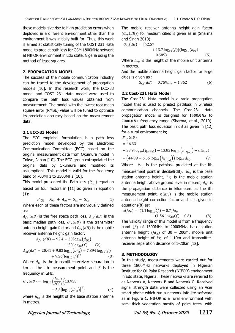
The mobile receiver antenna height gain factor

(𝐺𝑟𝑥(𝑑𝐵)) for medium cities is given as in (Sharma

and Singh 2010):

𝐺𝑟𝑥(𝑑𝐵) = [42.57

+ 13.7 log10(𝑓)](log10(ℎ𝑟𝑥)

− 0.585) (5)

Where ℎ𝑟𝑥 is the height of the mobile unit antenna

in metres.

And the mobile antenna height gain factor for large

cities is given as :

𝐺𝑟𝑥(𝑑𝐵) = 0.759ℎ𝑟𝑥 − 1.862 (6)

2.2 Cost-231 Hata Model

The Cost-231 Hata model is a radio propagation

model that is used to predict pathloss in wireless

communication channels. The Cost-231 Hata

propagation model is designed for 1500𝑀𝐻𝑧 to

2000𝑀𝐻𝑧 frequency range (Sharma, et.al., 2010).

The basic path loss equation in dB as given in [12]

for a rural environment is;

𝑃𝑙(𝑖)(𝑑𝐵)

= 46.33

+ 33.9 log10(𝑓[𝑀𝐻𝑧]) − 13.82 log10 (ℎ𝑡𝑥[𝑚]) − 𝑎(ℎ𝑟𝑥)

+ (44.99 − 6.55 log10 (ℎ𝑡𝑥[𝑚])) log10 𝑑(𝑖) (7)

Where 𝑃𝑙(𝑖) is the pathloss predicted at the ith

measurement point in decibel(dB), ℎ𝑡𝑥 is the base

station antenna height, ℎ𝑟𝑥 is the mobile station

antenna height above ground level in meters, 𝑑(𝑖) is

the propagation distance in kilometers at the ith

measurement point, a(ℎ𝑟𝑥) is the mobile station

antenna height correction factor and it is given in

equations(8) as;

𝑎(ℎ𝑟𝑥) = (1.1 log10(𝑓) − 0.7)ℎ𝑟𝑥− (1.56 log10(𝑓) − 0.8) (8)

The validity range of this model is from a frequency

band (𝑓) of 1500MHz to 2000MHz, base station

antenna height (ℎ𝑡𝑥) of 30 – 200m, mobile unit

antenna height of ℎ𝑟𝑥 of 1-10m and transmitter-

receiver separation distance of 1-20km [12].

3. METHODOLOGY

In this study, measurements were carried out for

three 1800MHz networks deployed in Nigerian

Institute for Oil Palm Research (NIFOR) environment

in Edo state, Nigeria. These networks are referred to

as Network A, Network B and Network C. Received

signal strength data were collected using an Acer

smart phone which run a network info lite software

as in Figure 1. NIFOR is a rural environment with

semi thick vegetation mostly of palm trees, with



scattered settlements as in the Google map Earth

view of Figure 2. Received Signal Strength data

(RSSL) was collected on active mode for a period of

120s at an interval of 100m due to the size of the

cells at a mobile antenna height of 1.5m for a period

of 6 months. RSSL data was collected for three radial

directions which corresponds to the three sectorial

antennas mounted at 120° to achieve 360° coverage.

In addition to RSSL data collected, base station

parameters collected were the base station antenna

height (ℎ𝑡𝑥)(𝑚) and the standard transmit power ′𝑃𝑡 ′

(𝑑𝐵).

Figure 1: A screen shot of the Network cell Info

Figure 2: Google map Earth view of lite software

interface NIFOR

4. RESULTS BEFORE TUNING

In propagation studies, there are several existing

empirical propagation models that can be used to

predict path loss in a rural environment. For this

study the ECC-33 model and the COST 231 Hata

model were used to compare the path loss (dB)

estimated from the measured received signal

strength data.

For easy comparison, a graphical plot showing the

measured and predicted path loss values for the

ECC-33 model and COST 231 Hata model plotted

with respect to distance for the Network A, B and C

with MATLAB_ R2017b software are given in Figure

3 through to Figure 5.

Figure 3: Plot of estimated path loss from measured data and path loss obtained from existing empirical models for Network A at 1800MHz in NIFOR, Edo

state.

Figure 4: Plot of estimated path loss from measured data and path loss obtained from existing empirical models for Network B at 1800MHz in NIFOR, Edo

state.

Figure 5: Plot of estimated path loss from measured data and path loss predicted from existing empirical models for Network C at 1800MHz in NIFOR, Edo

state.



5. MODEL VALIDATION BEFORE TUNING

The performance evaluation of a model is a vital

aspect of path loss prediction and essential to its

evaluation are the values of the goodness of fit

indices obtained from the analysis of the given

model. In this section, the COST 231 Hata model and

the ECC-33 models are validated to ascertain its

suitability for the Networks investigated. The Mean

Prediction Error (MPE) and Root Mean Square of

Errors (RMSE) in equation (9) and equation (10) are

used to evaluate the goodness of fit of these models,

and the computational results are presented in Table

1.

𝑀𝑃𝐸 =1

𝑛∑(𝑃𝑙𝑚(𝑖)

− 𝑃𝑙𝑝(𝑖))

𝑛

𝑖=1

(9)

𝑅𝑀𝑆𝐸 = √(∑(𝑃𝑙𝑝(𝑖) − 𝑃𝑙𝑚(𝑖)

)2

𝑛

𝑛

𝑖=1

) (10)

where n=number of measurement points, 𝑃𝑙𝑚(𝑖) is

the path loss estimated from measured data at the

ith measurement point and 𝑃𝑙𝑝(𝑖) is the path loss

predicted at the ith measurement point using the

COST 231 Hata Model and the ECC-33 model.

Based on the the error values in Table 1, the COST

231 Hata model has the minimum MPE and RMSE

values of Networks A, B and C. Thus, the COST 231

Hata model will be tuned to improve its prediction

accuracy.

6. TUNING OF COST-231 HATA MODEL

The high RMSE values obtained from the COST 231

Hata model is as a result of the different

characteristics of the environment in which this

model was built for. The least square tuning

approached as in [13] will be utilized in this study.

If the error term (𝑃𝑙𝑝(𝑖) − 𝑃𝑙𝑚(𝑖))2

in equation (10) can

be minimized, then the accuracy of predictions from

this model will improve. For the purpose of tuning,

let equation (7) be written as in equation (11) and

equation (12) as;

𝑃𝑙(𝑖)(𝑑𝐵)

= 46.33

+ 33.9 log10(𝑓[𝑀𝐻𝑧]) − 13.82 log10 (ℎ𝑡𝑥[𝑚]) − 𝑎(ℎ𝑟𝑥)

+ 44.99 log10 𝑑(𝑖)

− 6.55 log10 (ℎ𝑡𝑥[𝑚]) log10 𝑑(𝑖) (11)

𝑃𝑙(𝑖)(𝑑𝐵) = 𝐴1 + 𝐴3 log10(𝑓[𝑀𝐻𝑧])

− 𝐴4 log10 (ℎ𝑡𝑥[𝑚]) − 𝑎(ℎ𝑟𝑥)

+ 𝐴2 log10 𝑑(𝑖)

− 𝐴5 log10 (ℎ𝑡𝑥[𝑚]) log10 𝑑(𝑖) (12)

where 𝐴1 to 𝐴5 are the model tuning parameters.

For each measurement point, 𝑓, ℎ𝑡𝑥, ℎ𝑟𝑥 are fixed

values; but 𝑑(𝑖) is a variable, so the model tuning

mainly depend on 𝐴1 and 𝐴2.

Thus, the equation that needed to be tuned is;

∆𝐴= 𝐴1 + 𝐴2 log10 𝑑(𝑖) (13)

Assuming the error term 𝑃𝑙𝑝(𝑖) − 𝑃𝑙𝑚(𝑖)=𝐸𝑜(𝑖), then the

total error can be calculated as;

𝐸(𝐴1, 𝐴2) =∑(∆𝐴 − 𝐸𝑜(𝑖))2

𝑛

𝑖=1

(14)

Let

∆𝐴= 𝐶1 + 𝐶2 log10 𝑑(𝑖) (15)

Where 𝐶1 is the attenuation constant and 𝐶2 the

attenuation parameter about the distance 𝑑(𝑖).

By substituting the value of equation (15) in equation

(14),

𝐸(𝐶1, 𝐶2) = ∑(𝐶1 + 𝐶2 log10 𝑑(𝑖) − 𝐸𝑜(𝑖))2

𝑛

𝑖=1

(16)

According to linear least square theory [11], in order

to make sure that the value of error function

𝐸(𝐶1, 𝐶2) is minimum,

{

𝑑 𝐸(𝐶1, 𝐶2)

𝑑𝐶1= 0

𝑑 𝐸(𝐶1, 𝐶2)

𝑑𝐶2= 0

(17)

By substituting equation (16) in equation (17), and

evaluating it;

Table 1. Mean Prediction Error (MPE) and Root Mean Square Error (RMSE) values for Networks A, B and C

at 1800MHz

NETWORK Mean Prediction Error (MPE) Root Mean Square Error (RMSE)

ECC-33 Model Cost 231 Hata Model ECC-33 Model Cost 231 Hata Model

A 27.07 24.90 27.80 25.51

B 27.14 25.43 27.40 26.36

C 22.11 18.11 22.29 20.22



{

∑2(𝐶1 + 𝐶2 log10 𝑑(𝑖) − 𝐸𝑜(𝑖)) × 1

𝑛

𝑖=1

∑2(𝐶1 + 𝐶2 log10 𝑑(𝑖) − 𝐸𝑜(𝑖))

𝑛

𝑖=1

× log10 𝑑(𝑖)

= 0 (18)

This implies that,

∑(𝐶1 + 𝐶2 log10 𝑑(𝑖) − 𝐸𝑜(𝑖)) = 0

𝑛

𝑖=1

(19)

and

∑((𝐶1 + 𝐶2 log10 𝑑(𝑖) − 𝐸𝑜(𝑖)) × log10 𝑑(𝑖))

𝑛

𝑖=1

= 0 (20)

By re-positioning the elements, equations (19) and

(20) are expressed as;

𝑛𝐶1 + 𝐶2 (∑log𝑑(𝑖)

𝑛

𝑖=1

) =∑𝐸𝑜(𝑖)

𝑛

𝑖=1

(21)

𝐶1∑log𝑑(𝑖) + 𝐶2∑(log 𝑑(𝑖))2

𝑛

𝑖=1

𝑛

𝑖=1

=∑(𝐸𝑜(𝑖) × log 𝑑(𝑖))

𝑛

𝑖=1

(22)

From equation (21),

𝐶1 =∑ 𝐸𝑜(𝑖)𝑛𝑖=1 − 𝐶2(∑ log 𝑑(𝑖)

𝑛𝑖=1 )

𝑛 (23)

By substituting the value of 𝐶1 in equation (22),

(∑𝐸𝑜(𝑖)

𝑛

𝑖=1

− 𝐶2 (∑log 𝑑(𝑖)

𝑛

𝑖=1

)) ×∑log 𝑑(𝑖)

𝑛

𝑖=1

+ 𝑛𝐶2∑(log 𝑑(𝑖))2

𝑛

𝑖=1

= 𝑛∑(𝐸𝑜(𝑖) × log 𝑑(𝑖))

𝑛

𝑖=1

(24)

𝐶2

=𝑛∑ (𝐸𝑜(𝑖) × log 𝑑(𝑖)) − ∑ 𝐸𝑜(𝑖) × ∑ log 𝑑(𝑖)

𝑛𝑖=1

𝑛𝑖=1

𝑛𝑖=1

(𝑛 ∑ (log 𝑑(𝑖))𝑛𝑖=1 )

2− (∑ log 𝑑(𝑖)

𝑛𝑖=1 )

2 (25)

From equation (19),

𝐶2 =(∑ 𝐸𝑜(𝑖)

𝑛𝑖=1 ) − 𝑛𝐶1

∑ log 𝑑(𝑖)𝑛𝑖=1

By substituting the value of 𝐶2in equation (22),

𝐶1∑(log 𝑑(𝑖)) + ((∑ 𝐸𝑜(𝑖)

𝑛𝑖=1 ) − 𝑛𝐶1

∑ log 𝑑(𝑖)𝑛𝑖=1

)

𝑛

𝑖=1

×∑(log 𝑑(𝑖))2

𝑛

𝑖=1

=∑(𝐸𝑜(𝑖) × log𝑑(𝑖))

𝑛

𝑖=1

(26)

𝐶1 (∑(log 𝑑(𝑖))

𝑛

𝑖=1

)

2

+ (∑𝐸𝑜(𝑖)

𝑛

𝑖=1

) ×∑(log𝑑(𝑖))2

𝑛

𝑖=1

− (𝑛𝐶1)∑(log 𝑑(𝑖))2

𝑛

𝑖=1

=∑(𝐸𝑜(𝑖) × log 𝑑(𝑖))

𝑛

𝑖=1

× (∑(log 𝑑(𝑖))

𝑛

𝑖=1

) (27)

So

𝐶1 =𝐴 − 𝐵

𝐶 (28)

Where:

𝐴 = (∑𝐸𝑜(𝑖)

𝑛

𝑖=1

) ×∑(log 𝑑(𝑖))2

𝑛

𝑖=1

𝐵 =∑(𝐸𝑜(𝑖) × log 𝑑(𝑖))

𝑛

𝑖=1

× (∑(log 𝑑(𝑖))

𝑛

𝑖=1

)

and

𝐶 = 𝑛∑(log 𝑑(𝑖))2

𝑛

𝑖=1

− (∑(log 𝑑(𝑖))

𝑛

𝑖=1

)

2

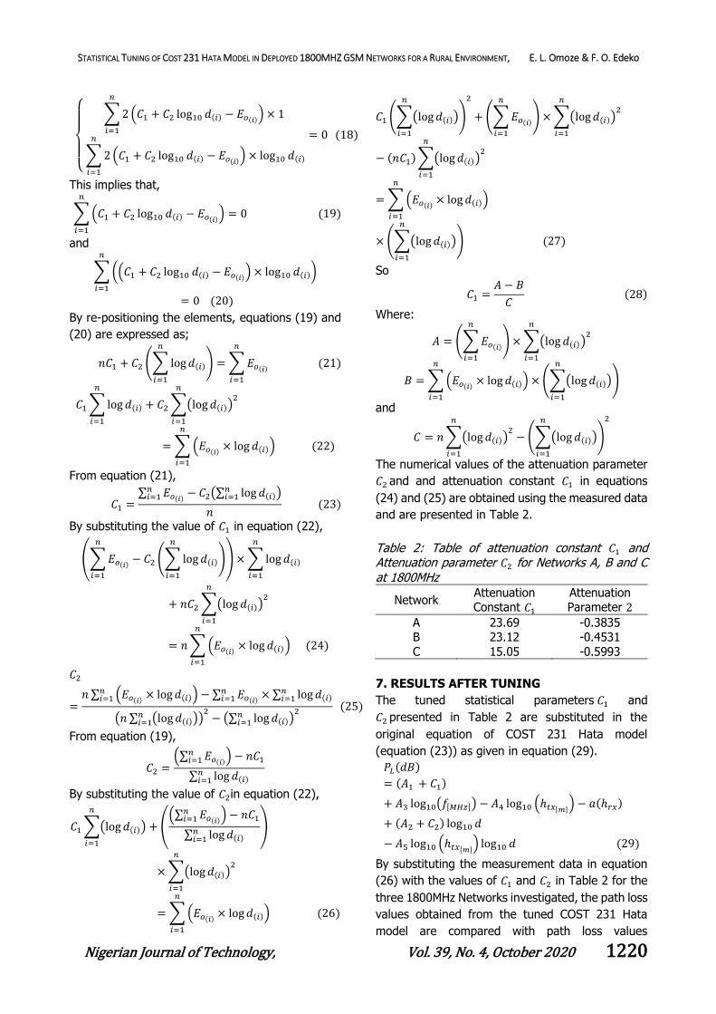
The numerical values of the attenuation parameter

𝐶2 and and attenuation constant 𝐶1 in equations

(24) and (25) are obtained using the measured data

and are presented in Table 2.

Table 2: Table of attenuation constant 𝐶1 and Attenuation parameter 𝐶2 for Networks A, B and C at 1800MHz

Network Attenuation Constant 𝐶1

Attenuation Parameter 2

A 23.69 -0.3835 B 23.12 -0.4531

C 15.05 -0.5993

7. RESULTS AFTER TUNING

The tuned statistical parameters 𝐶1 and

𝐶2 presented in Table 2 are substituted in the

original equation of COST 231 Hata model

(equation (23)) as given in equation (29).

𝑃𝐿(𝑑𝐵)

= (𝐴1 + 𝐶1)

+ 𝐴3 log10(𝑓[𝑀𝐻𝑧]) − 𝐴4 log10 (ℎ𝑡𝑥[𝑚]) − 𝑎(ℎ𝑟𝑥)

+ (𝐴2 + 𝐶2) log10 𝑑

− 𝐴5 log10 (ℎ𝑡𝑥[𝑚]) log10 𝑑 (29)

By substituting the measurement data in equation

(26) with the values of 𝐶1 and 𝐶2 in Table 2 for the

three 1800MHz Networks investigated, the path loss

values obtained from the tuned COST 231 Hata

model are compared with path loss values



estimated from measured received signal strength

using Matlab-R2017B software and presented

graphically as in Figure 6 through to Figure 8.

8. VALIDATION OF TUNED RESULTS

The validation of a model is a vital aspect of the

model tuning and essential to its evaluation are the

values of the goodness of fit indices obtained from

the analysis of the given model. In this section, the

tuned model is validated to ascertain its suitability

for the Networks investigated. The Mean Prediction

Error (MPE) and Root Mean Square of Errors

(RMSE) in equation (9) and equation (10) are used

to evaluate the goodness of fit of the developed

model, and the computational results are presented

in Table 3.

Table 3: Mean Prediction Error (MPE) and Root Mean Square Error (RMSE) values for Networks A,

B and C at 1800MHz with the Tuned COST 231 Hata model

NETWORK MPE (dB) RMSE (dB)

A 1.17 5.58 B 2.26 7.16

C 6.21 10.78

By comparing the values obtained in Table 1 with

that in Table 3 for the COST 231 Hata model,

equation (30) and equation (31) are used to

calculate the percentage decrease in MPE and RMSE

values.

Percentage decrease (MPE)

=𝐼𝑛𝑖𝑡𝑖𝑎𝑙 𝑣𝑎𝑙𝑢𝑒(𝑀𝑃𝐸) − 𝐹𝑖𝑛𝑎𝑙 𝑣𝑎𝑙𝑢𝑒(𝑀𝑃𝐸)

𝐼𝑛𝑖𝑡𝑖𝑎𝑙 𝑣𝑎𝑙𝑢𝑒(𝑀𝑃𝐸)× 100 (30)

Percentage decrease (RMSE)

=𝐼𝑛𝑖𝑡𝑖𝑎𝑙 𝑣𝑎𝑙𝑢𝑒(𝑅𝑀𝑆𝐸) − 𝐹𝑖𝑛𝑎𝑙 𝑣𝑎𝑙𝑢𝑒(𝑅𝑀𝑆𝐸)

𝐼𝑛𝑖𝑡𝑖𝑎𝑙 𝑣𝑎𝑙𝑢𝑒(𝑅𝑀𝑆𝐸)× 100 (31)

Figure 6: Plot of estimated path loss from

measured data and path loss predicted using the

tuned COST 231 Hata model for Network A at 1800MHz in NIFOR, Edo state.


measured data and path loss predicted using the tuned COST 231 Hata model for Network B at

1800MHz in NIFOR, Edo state.


measured data and path loss predicted using the tuned COST 231 Hata model for Network C at

1800MHz in NIFOR, Edo state.

Results of this computation show a percentage

decrease of MPE values of 95.30%, 91.11% and

65.71% for Networks A, B and C respectively. While

a percentage decrease of RMSE values of 78.13%,

72.84% and 46.69% was also obtained for Network

A, B and C respectively.

9. CONCLUSION

This paper presents a study into the characteristics

of radio signals for a rural environment (NIFOR) in

Benin City, Edo state, Nigeria. An experimental

campaign was conducted in the study environment

using three deployed GSM networks transmitting at



1800MHz. Received signal strength data was

collected using an Acer smart phone for three radial

directions for a period of 120 seconds in (dBm) for

a period of 6 months. Path loss was estimated from

the measured data using standard transmit power

values and compared with path loss predicted using

COST 231 Hata model and ECC-33 model. The

COST 231 Hata model equation was tuned using the

least square tuning approach. The tuned values of

the attenuation constant 𝐶1 and attenuation

parameter 𝐶2 obtained can be effectively applied to

the COST 231 Hata model equation for predicting

path loss. This is because of the low MPE and RMSE

values obtained. Results of the tuned COST 231

Hata model gave a percentage decrease of MPE

values of 95.30%, 91.11% and 65.71% for

Networks A, B and C respectively. While a

percentage decrease of RMSE values of 78.13%,

72.84% and 46.69% was also obtained for Network

A, B and C. The tuned COST 231 Hata model shows

better performance when compared to the original

COST 231 Hata model and it can be used to predict

path loss in environments with similar terrain

profile.

10. REFERENCES

[1] Ohaneme C.O., Onoh G.N., Ifeagwu E.N., and

Eneh, I.I. “Improving Channel Capacity of a Cellular System Using Cell Splitting”,

International Journal of Scientific & Engineering Research, Vol-03, issue- 5, Pp.1-8, 2012.

[2] Neskovic, A., Neskovic, N. and Paunovic, G. “Modern Approaches in Modelling of Mobile

Radio Systems Propagation Environment”,

IEEE Communications Surveys & Tutorials, Vol-03, issue-03, Pp 2-12, 2000.

[3] Struzak, R. Radio wave propagation basics, ICTP-ITU-URSI School on Wireless Networking for Development, Italy, 2006.

[4] Zhang, Y., Wen,J., Yang, G., et al. “Path Loss

Prediction Based on Machine Learning:

Principle, Method and Data Expansion”, Applied Sciences, Vol-09, Issue-09, 1908, 2019.

[5] Wen, J., Zhang, Y., Yang, G., et al, “Path Loss

Prediction Based on Machine Learning

Methods for Aircraft Cabin Environments”, IEEE Access, Vol-07, Pp 159251-159261,

2019.

[6] Hrovat, A., Javornik, T. Plevel, S., et al.

“Comparison of WIMAX Field Measurements and Empirical Path Loss Model in Urban and

Suburban Environment”, Proceedings of the 10th WSEAS International Conference on Communications, Vouliagmeni, Athens,

Greece, Pp 374-378, 2006.

[7] Sasaki, M., Nakamura, M., Yamada, W., et al.

“Path Loss Characteristics from 2 to 66GHz in Urban Macrocell Environments Based on

Analysis using ITU-R Site-General Models”,

12th European Conference on Antennas and Propagation, (EUCAP 2018). Pp 367-375,

2018. Doi:10.1049/cp.2018.0726.

[8] Salous, S., Lee, J., Kim, M.D., et al. ”Radio

Propagation Measurement and Modelling for Standardization of the Site General Path Loss

Model in International Telecommunications

Union Recommendations for 5G wireless networks”, Radio Science, Vol-55, Issue-01,

2020.

[9] Alam, M.D and Khan R.H. “Comparative Study

of Path Loss Models of WIMAX at 2.5GHz

Frequency Band”, International Journal of Future Generation Community and Networking, Vol.6, issue-02, pp 11-24, 2013.

[10] Akinbolati, A. and Agunbiade, O.J.,

“Assessment of Error Bounds for Path Loss

Prediction Models for TV White Space Usage in Ekiti State, Nigeria”, I.J Information Engineering and Electronic Business, Vol-03, Pp 28-39, 2020.

[11] Poppola, S.I., Atayero, A.A, Popoola, A.O., “Comparative Assessment of Data Obtained

Using Empirical Models for Path Loss

Predictions in a University Campus Environment”, Science Direct, Vol-18, Pp 380-

393, 2018.

[12] Onipe, J.A., Alenoghena, C.A., Salawu, N.et al.

“Optimal Propagation Models for Path-loss

Prediction in a Mountainous Environment at 2100MHz”, International Conference in Mathematics, Computer Engineering and Computer Science (ICMCECS). IEEE, Ayobo,

Ipaja, Lagos, Nigeria Pp 1-6, 2020.

[13] Yang, M. and Shi, W. “A Linear Least Square

Method of Propagation Model Tuning for 3G

Radio Network Planning” IEEE Fourth International Conference on Natural Computation-Jinan, Shandong, China, Pp 150-154, 2008.

Documents

STATISTICAL TUNING OF COST 231 HATA MODEL IN DEPLOYED