Embed Size (px)
Citation preview

Diagnosing systematic numerical weather prediction modelbias over the Antarctic from short-term forecast tendencies
Steven Cavallo1
ECMWF/WWRP Workshop: Model Uncertainty
12 April 2016
Reading, UK
1University of Oklahoma, School of Meteorology, Norman, OK
1 Background and methodAntarctic weather and climate predictionUsing ensemble data assimilation to diagnose sources ofmodel bias in a limited area model
2 Application to Antarctic numerical weather predictionModel and experimental setup
3 ResultsA-DART experimentsAdjustment from initial conditions
4 Summary and future work
Outline
1 Background and methodAntarctic weather and climate predictionUsing ensemble data assimilation to diagnose sources ofmodel bias in a limited area model
2 Application to Antarctic numerical weather predictionModel and experimental setup
3 ResultsA-DART experimentsAdjustment from initial conditions
4 Summary and future work
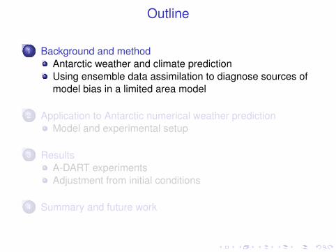
Antarctica: Why do we care?
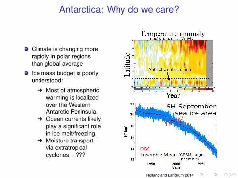
Climate is changing morerapidly in polar regionsthan global average
Ice mass budget is poorlyunderstood:
Ô Most of atmosphericwarming is localizedover the WesternAntarctic Peninsula.
Ô Ocean currents likelyplay a significant rolein ice melt/freezing.
Ô Moisture transportvia extratropicalcyclones = ???
Holland and Landrum 2014
Antarctica: Why do we care?
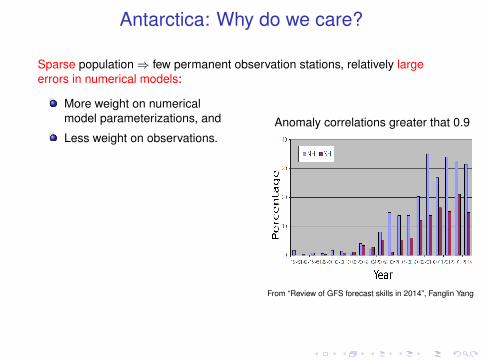
Sparse population⇒ few permanent observation stations, relatively largeerrors in numerical models:
More weight on numericalmodel parameterizations, and
Less weight on observations.
Result: Atmospheric analysesexhibit high uncertainty⇒ verydifficult to support scientific studieswith:
Ô atmospheric reanalyses,
Ô numerical models of theatmosphere,
Ô coupled numerical modelsthat depend on atmosphericforcings.
Anomaly correlations greater that 0.9
From “Review of GFS forecast skills in 2014”, Fanglin Yang
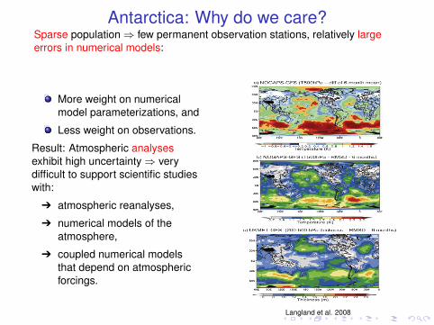
Antarctica: Why do we care?Sparse population⇒ few permanent observation stations, relatively largeerrors in numerical models:
More weight on numericalmodel parameterizations, and
Less weight on observations.
Result: Atmospheric analysesexhibit high uncertainty⇒ verydifficult to support scientific studieswith:
Ô atmospheric reanalyses,
Ô numerical models of theatmosphere,
Ô coupled numerical modelsthat depend on atmosphericforcings.
Langland et al. 2008
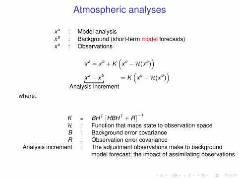
Atmospheric analyses
xa : Model analysisxb : Background (short-term model forecasts)xo : Observations
xa = xb + K(
xo −H(xb))
xa − xb
Analysis increment= K
(xo −H(xb)
)where:
K = BHT [HBHT + R]−1
H : Function that maps state to observation spaceB : Background error covarianceR : Observation error covariance
Analysis increment : The adjustment observations make to backgroundmodel forecast; the impact of assimilating observations
Can we use data assimilation to diagnose the precisesource of model error?
Klinker and Sardeshmukh (1992) and Rodwell and Palmer (2007):
Ô Mean analysis increment ' - mean model forecast tendency whenaveraged over many data assimilation cycles.
Ô For stationary systems, a non-zero analysis increment⇒divergence of model state from observations via the modelforecast tendencies.
Ô Good initial analysis→ model errors that develop in the earlystages of a forecast simulation must be associated with errors inthe model parameterizations of atmospheric processes (See alsoWlliams and Brooks 2008; Xie et al. 2012; Williams et al. 2013).
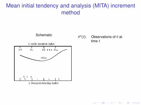
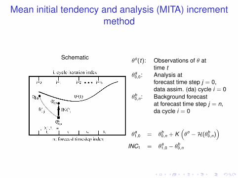
Mean initial tendency and analysis (MITA) incrementmethod
Schematicθo(t): Observations of θ at
time t
θa0,0: Analysis at
forecast time step j = 0,data assim. (da) cycle i = 0
θb0,n: Background forecast
at forecast time step j = n,da cycle i = 0
Mean initial tendency and analysis (MITA) incrementmethod
Schematicθo(t): Observations of θ at
time tθa
0,0: Analysis atforecast time step j = 0,data assim. (da) cycle i = 0
θb0,n: Background forecast
at forecast time step j = n,da cycle i = 0
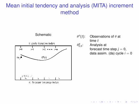
Mean initial tendency and analysis (MITA) incrementmethod
Schematicθo(t): Observations of θ at
time tθa
0,0: Analysis atforecast time step j = 0,data assim. (da) cycle i = 0
θb0,n: Background forecast
at forecast time step j = n,da cycle i = 0
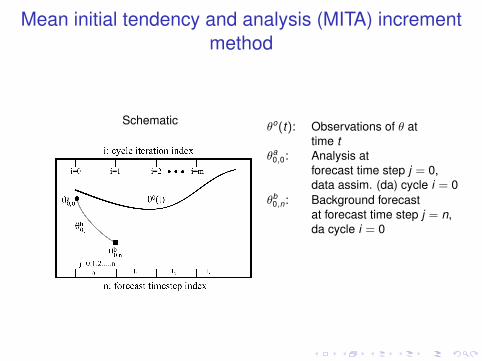
Mean initial tendency and analysis (MITA) incrementmethod
Schematicθo(t): Observations of θ at
time tθa
0,0: Analysis atforecast time step j = 0,data assim. (da) cycle i = 0
θb0,n: Background forecast
at forecast time step j = n,da cycle i = 0
θa1,0 = θb
0,n + K(θo −H(θb
0,n))
INC1 = θa1,0 − θb
0,n
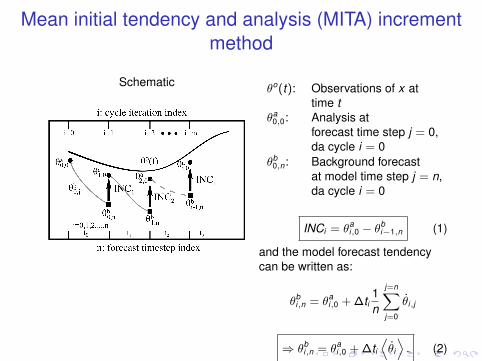
Mean initial tendency and analysis (MITA) incrementmethod
Schematicθo(t): Observations of x at
time tθa
0,0: Analysis atforecast time step j = 0,da cycle i = 0
θb0,n: Background forecast
at model time step j = n,da cycle i = 0
INCi = θai,0 − θb
i−1,n (1)
and the model forecast tendencycan be written as:
θbi,n = θa
i,0 + ∆ti1n
j=n∑j=0
θ̇i,j
⇒ θbi,n = θa
i,0 + ∆ti⟨θ̇i
⟩. (2)
Mean initial tendency and analysis (MITA) incrementmethod
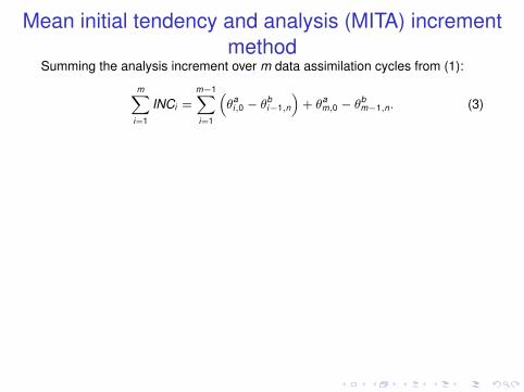
Summing the analysis increment over m data assimilation cycles from (1):
m∑i=1
INCi =m−1∑i=1
(θa
i,0 − θbi−1,n
)+ θa
m,0 − θbm−1,n. (3)
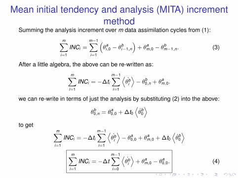
After a little algebra, the above can be re-written as:
m∑i=1
INCi = −∆tim−1∑i=1
⟨θ̇b
i
⟩− θb
0,n + θam,0.
we can re-write in terms of just the analysis by substituting (2) into the above:
θb0,n = θa
0,0 + ∆t0⟨θ̇b
0
⟩to get
m∑i=1
INCi = −∆tim−1∑i=1
⟨θ̇b
i
⟩− θa
0,0 + θam,0 + ∆t0
⟨θ̇b
0
⟩m∑
i=1
INCi = −∆tm−1∑i=0
⟨θ̇b
i
⟩+ θa
m,0 − θa0,0. (4)
Mean initial tendency and analysis (MITA) incrementmethod
Summing the analysis increment over m data assimilation cycles from (1):
m∑i=1
INCi =m−1∑i=1
(θa
i,0 − θbi−1,n
)+ θa
m,0 − θbm−1,n. (3)
After a little algebra, the above can be re-written as:
m∑i=1
INCi = −∆tim−1∑i=1
⟨θ̇b
i
⟩− θb
0,n + θam,0.
we can re-write in terms of just the analysis by substituting (2) into the above:
θb0,n = θa
0,0 + ∆t0⟨θ̇b
0
⟩to get
m∑i=1
INCi = −∆tim−1∑i=1
⟨θ̇b
i
⟩− θa
0,0 + θam,0 + ∆t0
⟨θ̇b
0
⟩m∑
i=1
INCi = −∆tm−1∑i=0
⟨θ̇b
i
⟩+ θa
m,0 − θa0,0. (4)
Mean initial tendency and analysis (MITA) incrementmethod
m∑i=1
INCi = −∆tm−1∑i=0
⟨θ̇b
i
⟩+ θa
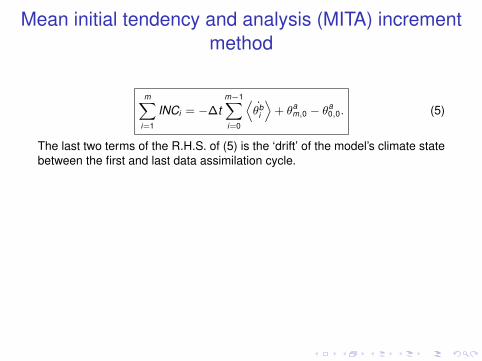
m,0 − θa0,0. (5)
The last two terms of the R.H.S. of (5) is the ‘drift’ of the model’s climate statebetween the first and last data assimilation cycle.
If the weather at the beginning and end of the data assimilation cycling issimilar, then from (5):
m∑i=1
INCi ' −∆tim−1∑i=0
⟨θ̇b
i
⟩(6)
⇒ INC = −∆tdaθ̇bi (7)
when averaged over m data assimilation cycles where ∆tda is the time stepbetween da cycles (usually 6 hours).
Mean initial tendency and analysis (MITA) incrementmethod
m∑i=1
INCi = −∆tm−1∑i=0
⟨θ̇b
i
⟩+ θa
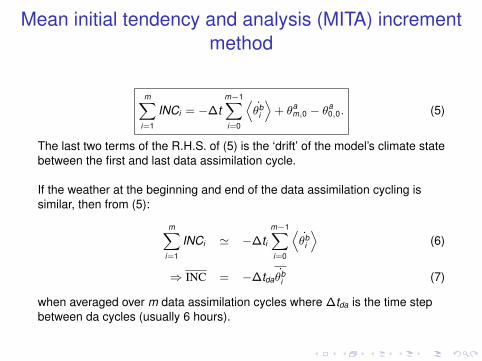
m,0 − θa0,0. (5)
The last two terms of the R.H.S. of (5) is the ‘drift’ of the model’s climate statebetween the first and last data assimilation cycle.
If the weather at the beginning and end of the data assimilation cycling issimilar, then from (5):
m∑i=1
INCi ' −∆tim−1∑i=0
⟨θ̇b
i
⟩(6)
⇒ INC = −∆tdaθ̇bi (7)
when averaged over m data assimilation cycles where ∆tda is the time stepbetween da cycles (usually 6 hours).
Other studies using the (MITA) method
Kay et al. 2011: Diagnosed unrealistic cloud increases over the Arcticusing Community Atmosphere Model (CAM).
Cloud-Associated Parameterizations Testbed: ‘CAPT’
Ô Deficiencies in climate models can not be identified simply byanalyzing climate statistics (e.g. Phillips et al. 2004; Williamson etal. 2005; Williamson and Olson 2007; Hannay et al. 2009;Medeiros et al. 2012).
Ô Must initialize forecasts from analyses produced with anothermodel, and thus first few days of forecasts show inconsistenciesbetween model and analysis instead of the true model bias.
Best when analysis used to initialize a forecast is produced by a dataassimilation system using the same model (Rodwell and Palmer 2007)
Although MITA has been applied in global models and by operationalcenters (i.e. ECMWF; Rodwell and Jung 2008) and Met Office UnifiedModel (Martin et al. 2010), it has never been applied to a limited areamodel.
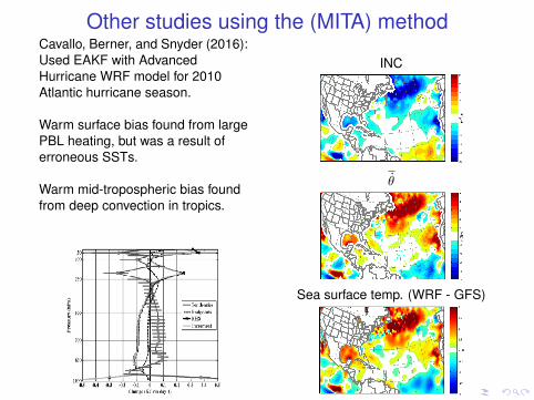
Other studies using the (MITA) methodCavallo, Berner, and Snyder (2016):Used EAKF with AdvancedHurricane WRF model for 2010Atlantic hurricane season.
Warm surface bias found from largePBL heating, but was a result oferroneous SSTs.
Warm mid-tropospheric bias foundfrom deep convection in tropics.
INC
θ̇
Sea surface temp. (WRF - GFS)
Hypothesis
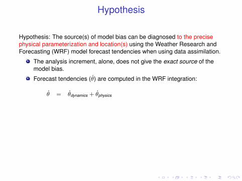
Hypothesis: The source(s) of model bias can be diagnosed to the precisephysical parameterization and location(s) using the Weather Research andForecasting (WRF) model forecast tendencies when using data assimilation.
The analysis increment, alone, does not give the exact source of themodel bias.
Forecast tendencies (θ̇) are computed in the WRF integration:
θ̇ = θ̇dynamics + θ̇physics
= θ̇dynamics +[θ̇radiation + θ̇pbl + θ̇cumulus + θ̇microphysics
]
The above budget can be completely closed using WRF
If the largest adjustment is expected in the first few time steps, do weonly need a fraction of the time steps to diagnose the model error?
Hypothesis
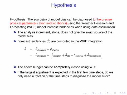
Hypothesis: The source(s) of model bias can be diagnosed to the precisephysical parameterization and location(s) using the Weather Research andForecasting (WRF) model forecast tendencies when using data assimilation.
The analysis increment, alone, does not give the exact source of themodel bias.
Forecast tendencies (θ̇) are computed in the WRF integration:
θ̇ = θ̇dynamics + θ̇physics
= θ̇dynamics +[θ̇radiation + θ̇pbl + θ̇cumulus + θ̇microphysics
]
The above budget can be completely closed using WRF
If the largest adjustment is expected in the first few time steps, do weonly need a fraction of the time steps to diagnose the model error?
Hypothesis
Hypothesis: The source(s) of model bias can be diagnosed to the precisephysical parameterization and location(s) using the Weather Research andForecasting (WRF) model forecast tendencies when using data assimilation.
The analysis increment, alone, does not give the exact source of themodel bias.
Forecast tendencies (θ̇) are computed in the WRF integration:
θ̇ = θ̇dynamics + θ̇physics
= θ̇dynamics +[θ̇radiation + θ̇pbl + θ̇cumulus + θ̇microphysics
]
The above budget can be completely closed using WRF
If the largest adjustment is expected in the first few time steps, do weonly need a fraction of the time steps to diagnose the model error?
Outline
1 Background and methodAntarctic weather and climate predictionUsing ensemble data assimilation to diagnose sources ofmodel bias in a limited area model
2 Application to Antarctic numerical weather predictionModel and experimental setup
3 ResultsA-DART experimentsAdjustment from initial conditions
4 Summary and future work
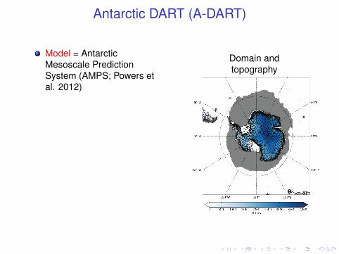
Antarctic DART (A-DART)
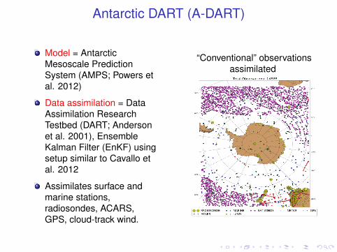
Model = AntarcticMesoscale PredictionSystem (AMPS; Powers etal. 2012)
Data assimilation = DataAssimilation ResearchTestbed (DART; Andersonet al. 2001), EnsembleKalman Filter (EnKF) usingsetup similar to Cavallo etal. 2012
Assimilates surface andmarine stations,radiosondes, ACARS,GPS, cloud-track wind.
Domain andtopography
Antarctic DART (A-DART)
Model = AntarcticMesoscale PredictionSystem (AMPS; Powers etal. 2012)
Data assimilation = DataAssimilation ResearchTestbed (DART; Andersonet al. 2001), EnsembleKalman Filter (EnKF) usingsetup similar to Cavallo etal. 2012
Assimilates surface andmarine stations,radiosondes, ACARS,GPS, cloud-track wind.
“Conventional” observationsassimilated
Antarctic DART (A-DART)
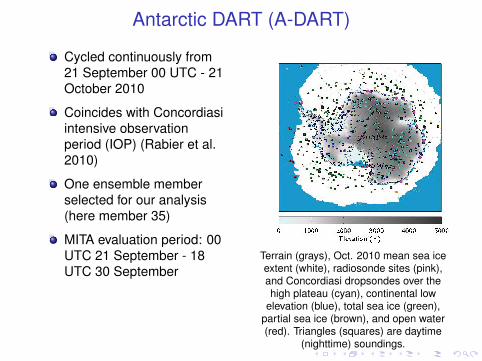
Cycled continuously from21 September 00 UTC - 21October 2010
Coincides with Concordiasiintensive observationperiod (IOP) (Rabier et al.2010)
One ensemble memberselected for our analysis(here member 35)
MITA evaluation period: 00UTC 21 September - 18UTC 30 September
Terrain (grays), Oct. 2010 mean sea iceextent (white), radiosonde sites (pink),and Concordiasi dropsondes over thehigh plateau (cyan), continental low
elevation (blue), total sea ice (green),partial sea ice (brown), and open water(red). Triangles (squares) are daytime
(nighttime) soundings.
Summary of A-DART
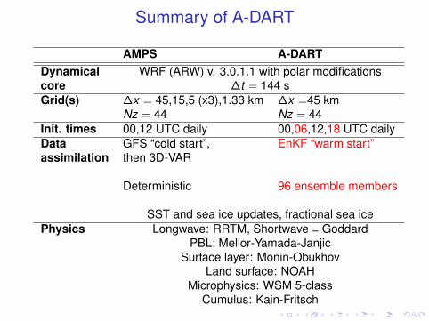
AMPS A-DARTDynamical WRF (ARW) v. 3.0.1.1 with polar modificationscore ∆t = 144 sGrid(s) ∆x = 45,15,5 (x3),1.33 km ∆x =45 km
Nz = 44 Nz = 44Init. times 00,12 UTC daily 00,06,12,18 UTC dailyData GFS “cold start”, EnKF “warm start”assimilation then 3D-VAR
Deterministic 96 ensemble members
SST and sea ice updates, fractional sea icePhysics Longwave: RRTM, Shortwave = Goddard
PBL: Mellor-Yamada-JanjicSurface layer: Monin-Obukhov
Land surface: NOAHMicrophysics: WSM 5-class
Cumulus: Kain-Fritsch
Antarctic DART (A-DART)
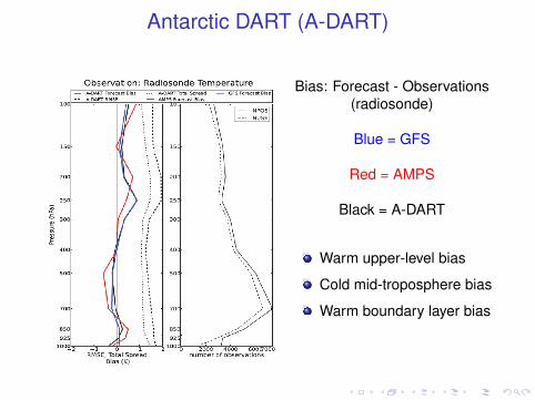
Bias: Forecast - Observations(radiosonde)
Blue = GFS
Red = AMPS
Black = A-DART
Warm upper-level bias
Cold mid-troposphere bias
Warm boundary layer bias
Antarctic DART (A-DART)
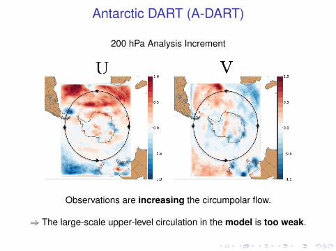
200 hPa Analysis Increment
Observations are increasing the circumpolar flow.
⇒ The large-scale upper-level circulation in the model is too weak.
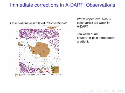
Immediate corrections in A-DART: Observations
Observations assimilated: “Conventional”Warm upper-level bias⇒polar vortex too weak inA-DART
Too weak of anequator-to-pole temperaturegradient.
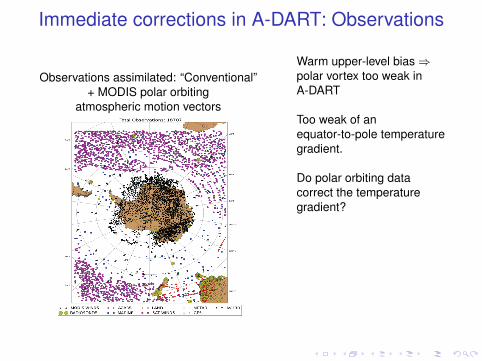
Immediate corrections in A-DART: Observations
Observations assimilated: “Conventional”+ MODIS polar orbiting
atmospheric motion vectors
Warm upper-level bias⇒polar vortex too weak inA-DART
Too weak of anequator-to-pole temperaturegradient.
Do polar orbiting datacorrect the temperaturegradient?
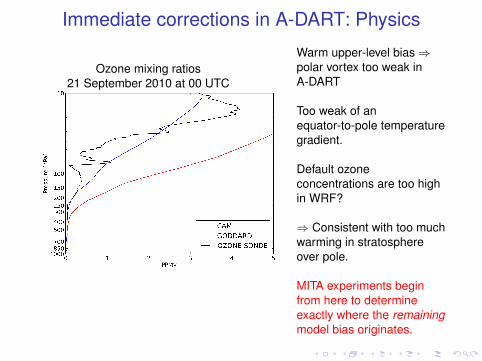
Immediate corrections in A-DART: Physics
Ozone mixing ratios21 September 2010 at 00 UTC
Warm upper-level bias⇒polar vortex too weak inA-DART
Too weak of anequator-to-pole temperaturegradient.
Default ozoneconcentrations are too highin WRF?
⇒ Consistent with too muchwarming in stratosphereover pole.
MITA experiments beginfrom here to determineexactly where the remainingmodel bias originates.
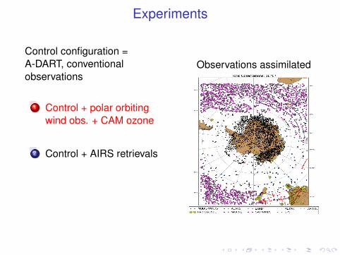
Experiments
Control configuration =A-DART, conventionalobservations
1 Control + polar orbitingwind obs. + CAM ozone
2 Control + AIRS retrievals
Observations assimilated
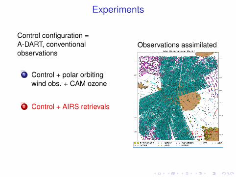
Experiments
Control configuration =A-DART, conventionalobservations
1 Control + polar orbitingwind obs. + CAM ozone
2 Control + AIRS retrievals
Observations assimilated
Outline
1 Background and methodAntarctic weather and climate predictionUsing ensemble data assimilation to diagnose sources ofmodel bias in a limited area model
2 Application to Antarctic numerical weather predictionModel and experimental setup
3 ResultsA-DART experimentsAdjustment from initial conditions
4 Summary and future work
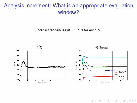
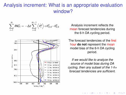
Analysis increment: What is an appropriate evaluationwindow?
Forecast tendencies at 850 hPa for each ∆t
θ̇(t) θ̇(t)physics
Analysis increment: What is an appropriate evaluationwindow?
m∑i=1
INCi = −∆tm−1∑i=0
⟨θ̇b
i
⟩+θa
m,0−θa0,0
Analysis increment reflects themean forecast tendencies during
the 6-h DA cycling period.
The forecast tendencies of the firsthour do not represent the meanmodel bias of the 6-h DA cycling
period.
If we would like to analyze thesource of model bias during DA
cycling, then any subset of the 1-h+forecast tendencies are sufficient.
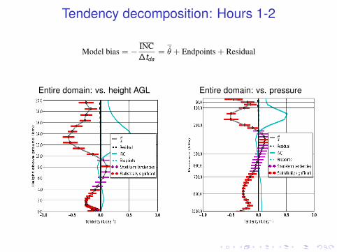
Tendency decomposition: Hours 1-2
Model bias = − INC∆tda
= θ̇ + Endpoints + Residual
Entire domain: vs. height AGL Entire domain: vs. pressure
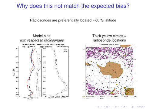
Why does this not match the expected bias?
Radiosondes are preferentially located ∼60◦S latitude
Model biaswith respect to radiosondes
Thick yellow circles =radiosonde locations
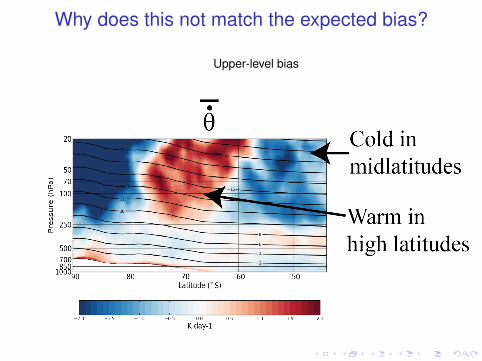
Why does this not match the expected bias?
Upper-level bias
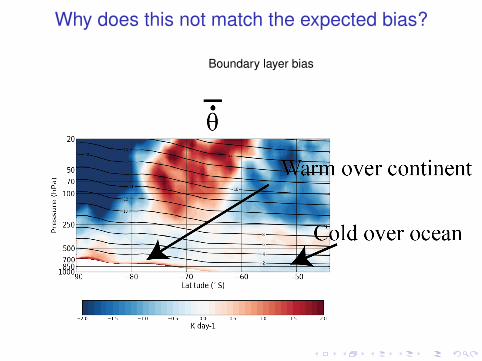
Why does this not match the expected bias?
Boundary layer bias
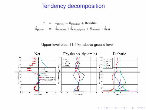
Tendency decomposition
θ̇ = θ̇physics + θ̇dynamics + Residual
θ̇physics = θ̇radiation + θ̇microphysics + θ̇cumulus + θ̇PBL
Upper-level bias: 11.4 km above ground level
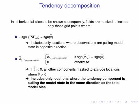
Tendency decomposition
In all horizontal slices to be shown subsequently, fields are masked to includeonly those grid points where:
- sgn(INCi,j
)= sgn(θ̇)
Ô Includes only locations where observations are pulling modelstate in opposite direction.
θ̇i,j (any component) =
{θ̇i,j (any component) if sgn(θ̇i,j ) = sgn(θ̇)
0 otherwise
Ô If θ̇ < 0, all other components masked to exclude locationswhere θ̇ > 0
Ô Includes only locations where the tendency component ispulling the model state in the same direction as the totalmodel bias.
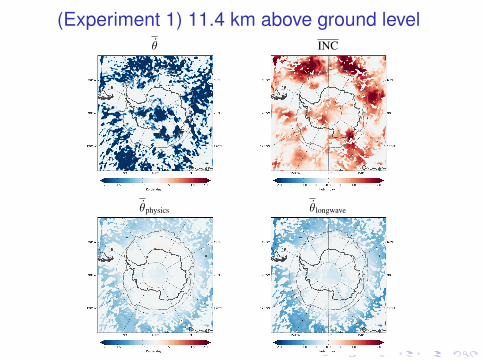
(Experiment 1) 11.4 km above ground levelθ̇ INC
θ̇physics θ̇longwave
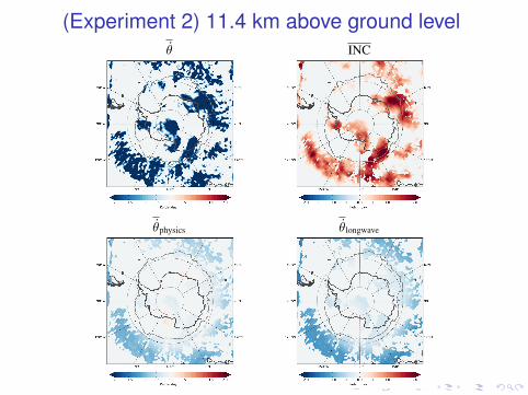
(Experiment 2) 11.4 km above ground levelθ̇ INC
θ̇physics θ̇longwave
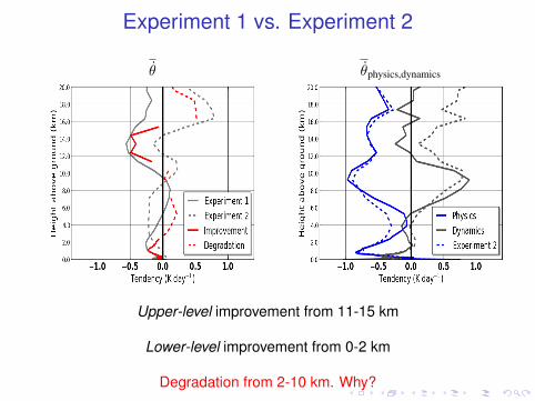
Experiment 1 vs. Experiment 2
θ̇ θ̇physics,dynamics
Upper-level improvement from 11-15 km
Lower-level improvement from 0-2 km
Degradation from 2-10 km. Why?
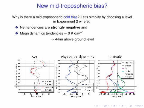
New mid-tropospheric bias?
Why is there a mid-tropospheric cold bias? Let’s simplify by choosing a levelin Experiment 2 where:
Net tendencies are strongly negative and
Mean dynamics tendencies ∼ 0 K day−1
⇒ 4-km above ground level
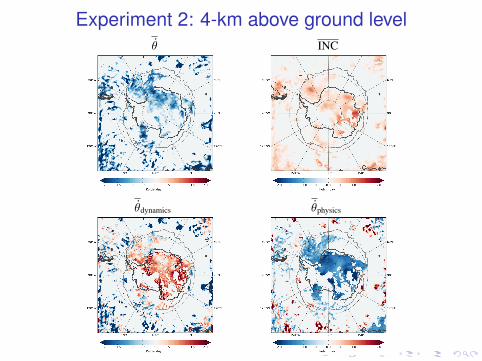
Experiment 2: 4-km above ground levelθ̇ INC
θ̇dynamics θ̇physics
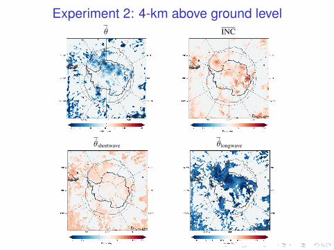
Experiment 2: 4-km above ground levelθ̇ INC
θ̇shortwave θ̇longwave
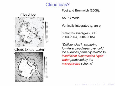
Cloud bias?Fogt and Bromwich (2008):
AMPS model
Vertically integrated qc an qi
6 months averages (DJF2003-2004, 2004-2005)
“Deficiencies in capturinglow-level cloudiness over coldice surfaces primarily related toinsufficient supercooled liquidwater produced by themicrophysics scheme”
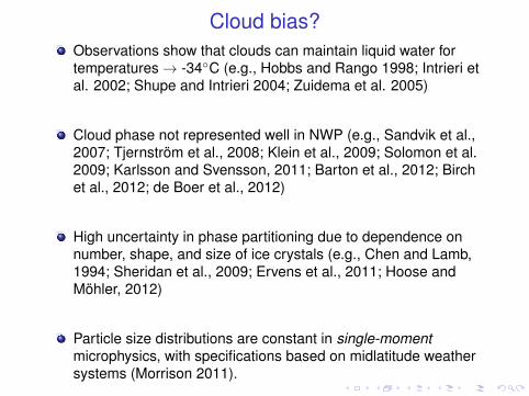
Cloud bias?Observations show that clouds can maintain liquid water fortemperatures→ -34◦C (e.g., Hobbs and Rango 1998; Intrieri etal. 2002; Shupe and Intrieri 2004; Zuidema et al. 2005)
Cloud phase not represented well in NWP (e.g., Sandvik et al.,2007; Tjernström et al., 2008; Klein et al., 2009; Solomon et al.2009; Karlsson and Svensson, 2011; Barton et al., 2012; Birchet al., 2012; de Boer et al., 2012)
High uncertainty in phase partitioning due to dependence onnumber, shape, and size of ice crystals (e.g., Chen and Lamb,1994; Sheridan et al., 2009; Ervens et al., 2011; Hoose andMöhler, 2012)
Particle size distributions are constant in single-momentmicrophysics, with specifications based on midlatitude weathersystems (Morrison 2011).
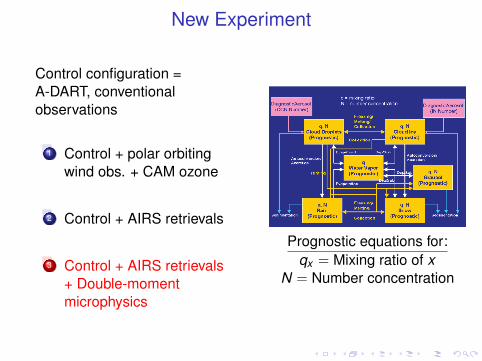
New Experiment
Control configuration =A-DART, conventionalobservations
1 Control + polar orbitingwind obs. + CAM ozone
2 Control + AIRS retrievals
3 Control + AIRS retrievals+ Double-momentmicrophysics
Prognostic equations for:qx = Mixing ratio of x
N = Number concentration
Experiment 2 vs. Experiment 3
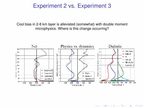
Cool bias in 2-8 km layer is alleviated (somewhat) with double momentmicrophysics. Where is this change occurring?
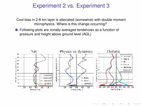
Experiment 2 vs. Experiment 3
Cool bias in 2-8 km layer is alleviated (somewhat) with double momentmicrophysics. Where is this change occurring?
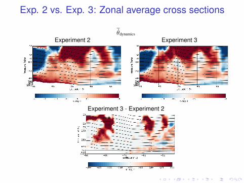
Following plots are zonally averaged tendencies as a function ofpressure and height above ground level (AGL)
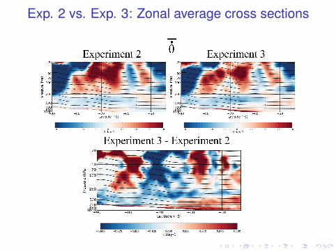
Exp. 2 vs. Exp. 3: Zonal average cross sections
Exp. 2 vs. Exp. 3: Zonal average cross sections
Exp. 2 vs. Exp. 3: Zonal average cross sections
θ̇dynamics
Experiment 2 Experiment 3
Experiment 3 - Experiment 2
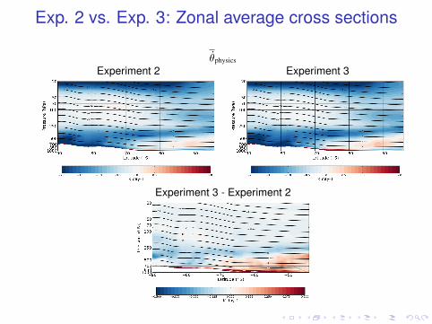
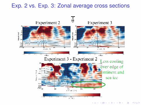
Exp. 2 vs. Exp. 3: Zonal average cross sections
θ̇physics
Experiment 2 Experiment 3
Experiment 3 - Experiment 2
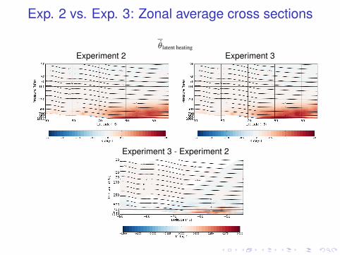
Exp. 2 vs. Exp. 3: Zonal average cross sections
θ̇latent heating
Experiment 2 Experiment 3
Experiment 3 - Experiment 2
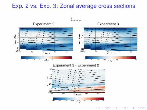
Exp. 2 vs. Exp. 3: Zonal average cross sections
θ̇radiation
Experiment 2 Experiment 3
Experiment 3 - Experiment 2
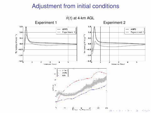
Adjustment from initial conditions
θ̇(t) at 4-km AGLExperiment 1 Experiment 2
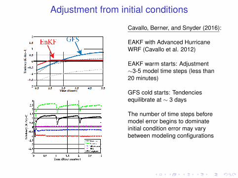
Adjustment from initial conditions
Cavallo, Berner, and Snyder (2016):
EAKF with Advanced HurricaneWRF (Cavallo et al. 2012)
EAKF warm starts: Adjustment∼3-5 model time steps (less than20 minutes)
GFS cold starts: Tendenciesequilibrate at ∼ 3 days
The number of time steps beforemodel error begins to dominateinitial condition error may varybetween modeling configurations
Outline
1 Background and methodAntarctic weather and climate predictionUsing ensemble data assimilation to diagnose sources ofmodel bias in a limited area model
2 Application to Antarctic numerical weather predictionModel and experimental setup
3 ResultsA-DART experimentsAdjustment from initial conditions
4 Summary and future work
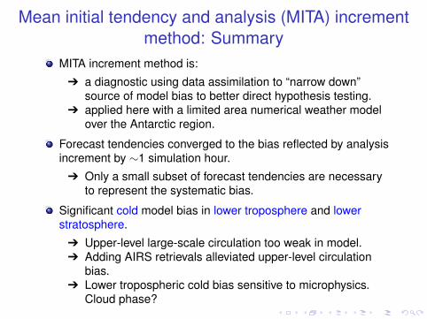
Mean initial tendency and analysis (MITA) incrementmethod: Summary
MITA increment method is:
Ô a diagnostic using data assimilation to “narrow down”source of model bias to better direct hypothesis testing.
Ô applied here with a limited area numerical weather modelover the Antarctic region.
Forecast tendencies converged to the bias reflected by analysisincrement by ∼1 simulation hour.
Ô Only a small subset of forecast tendencies are necessaryto represent the systematic bias.
Significant cold model bias in lower troposphere and lowerstratosphere.
Ô Upper-level large-scale circulation too weak in model.Ô Adding AIRS retrievals alleviated upper-level circulation
bias.Ô Lower tropospheric cold bias sensitive to microphysics.
Cloud phase?