Embed Size (px)
Citation preview

Working Paper Series
Stock Market Uncertainty and the Relation between Stock andBond Returns
Chris Stivers and Licheng Sun
Working Paper 2002-3March 2002

We thank Jennifer Conrad, Jerry Dwyer, Mark Fisher, Bill Lastrapes, Marc Lipson, Joe Sinkey, and seminar participantsfrom the Federal Reserve Bank of Atlanta, Emory University, Georgia Tech, Georgia State, and the University of Georgiafor comments and helpful discussions. The views expressed here are the authors’ and not necessarily those of the FederalReserve Bank of Atlanta or the Federal Reserve System. Any remaining errors are the authors’ responsibility.
Please address questions regarding content to Chris Stivers, Department of Banking and Finance, Brooks Hall, Terry Collegeof Business, University of Georgia, Athens, Georgia 30602 and Federal Reserve Bank of Atlanta (visiting scholar), 706-542-3648, 706-542-9434 (fax), [email protected], or Licheng Sun, Department of Banking and Finance, Brooks Hall,Terry College of Business, University of Georgia, Athens, Georgia 30602, 706-542-3661, 706-542-9434 (fax),[email protected].
The full text of Federal Reserve Bank of Atlanta working papers, including revised versions, is available on the Atlanta Fed’sWeb site at http://www.frbatlanta.org. Click on the “Publications” tab and then “Working Papers” in the navigation bar. Toreceive notification about new papers, please use the on-line publications order form, or contact the Public AffairsDepartment, Federal Reserve Bank of Atlanta, 1000 Peachtree Street, N.E., Atlanta, Georgia 30309-4470, 404-498-8020.
Federal Reserve Bank of AtlantaWorking Paper 2002-3
March 2002
Stock Market Uncertainty and the Relationbetween Stock and Bond Returns
Chris Stivers, University of GeorgiaLicheng Sun, University of Georgia
Abstract: The authors examine how the co-movement between daily stock and Treasury bond returns varieswith stock market uncertainty. They use the lagged implied volatility from equity index options to provide anobjective, observable, and dynamic measure of stock market uncertainty. The authors find that stock and bondreturns tend to move substantially together during periods of lower stock market uncertainty. However, stockand bond returns tend to exhibit little relation or even a negative relation during periods of high stock marketuncertainty. The authors’ findings have implications for understanding joint cross-market price formation.Further, their findings imply that diversification benefits increase for portfolios of stocks and bonds duringperiods of high stock market uncertainty.
JEL classification: G11, G12, G14
Key words: stock and bond market return linkages, stock market uncertainty, time-varying volatility

Stock market uncertainty and the relation
between stock and bond returns
1 Introduction
It is well known that stock-market volatility exhibits substantial variation over time. Further, this
variation in stock volatility is puzzling because it seems excessive based on the time-variation in
the volatility of fundamental economic variables (e.g., Schwert, 1989; Haugen, Talmor, and Torous,
1991; Whitelaw, 1994; Campbell, Lettau, Malkiel, and Xu, 2001).
It is also well known that stock and bond returns are positively correlated. However, the
unconditional correlation is small and a second body of research has tried to understand the co-
movements between the stock and bond markets (e.g., Barsky, 1989; Fama and French, 1989; Shiller
and Beltratti, 1992; Campbell and Ammer, 1993; and Fleming, Kirby, and Ostdiek, 1998).
In this paper, we are interested in the natural question of whether stock market uncertainty
has a role in understanding stock and bond market co-movements. If the relative attractiveness of
bonds versus stocks changes with stock market uncertainty, then the co-movement between stock
and bond returns may vary with stock market uncertainty. Changes in return co-movements might
be due to changing fundamentals (Campbell and Ammer, 1993), cross-market hedging (Fleming,
Kirby, and Ostdiek, 1998), or pricing influences related to time-varying economic uncertainty and
possible regime shifting (Veronesi, 1999 and 2001).
The idea that economic uncertainty and unobservable regime-shifting may be important in
understanding return dynamics seems related to the notion of “flight-to-quality” that is often sug-
gested in the popular press. The notion of flight-to-quality suggests that during times of increased
stock uncertainty: (1) the price of U.S. Treasury bonds tends to increase, relative to stocks; and
(2) the return co-movement between stocks and bonds becomes less positively correlated (or even
negatively correlated). For example, an article in the Wall Street Journal on 11/4/97 (around the
Asian financial crisis) speculates that the recent decoupling between the stock and bond markets
may be due to the high stock volatility and uncertain economic times. Or, in the Wall Street
Journal of 10/17/89, an article about the bond market states, “The sudden flight-to-quality that
1
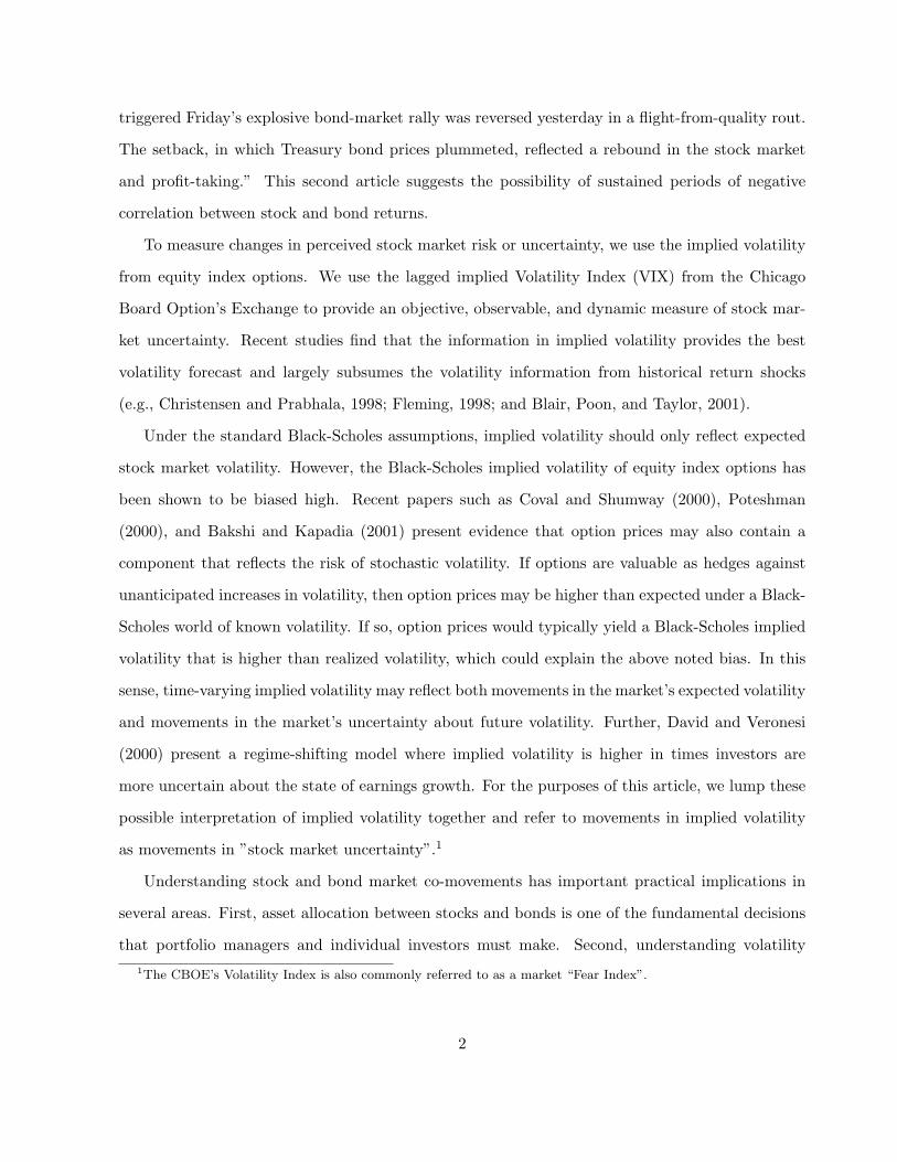
triggered Friday’s explosive bond-market rally was reversed yesterday in a flight-from-quality rout.
The setback, in which Treasury bond prices plummeted, reflected a rebound in the stock market
and profit-taking.” This second article suggests the possibility of sustained periods of negative
correlation between stock and bond returns.
To measure changes in perceived stock market risk or uncertainty, we use the implied volatility
from equity index options. We use the lagged implied Volatility Index (VIX) from the Chicago
Board Option’s Exchange to provide an objective, observable, and dynamic measure of stock mar-
ket uncertainty. Recent studies find that the information in implied volatility provides the best
volatility forecast and largely subsumes the volatility information from historical return shocks
(e.g., Christensen and Prabhala, 1998; Fleming, 1998; and Blair, Poon, and Taylor, 2001).
Under the standard Black-Scholes assumptions, implied volatility should only reflect expected
stock market volatility. However, the Black-Scholes implied volatility of equity index options has
been shown to be biased high. Recent papers such as Coval and Shumway (2000), Poteshman
(2000), and Bakshi and Kapadia (2001) present evidence that option prices may also contain a
component that reflects the risk of stochastic volatility. If options are valuable as hedges against
unanticipated increases in volatility, then option prices may be higher than expected under a Black-
Scholes world of known volatility. If so, option prices would typically yield a Black-Scholes implied
volatility that is higher than realized volatility, which could explain the above noted bias. In this
sense, time-varying implied volatility may reflect both movements in the market’s expected volatility
and movements in the market’s uncertainty about future volatility. Further, David and Veronesi
(2000) present a regime-shifting model where implied volatility is higher in times investors are
more uncertain about the state of earnings growth. For the purposes of this article, we lump these
possible interpretation of implied volatility together and refer to movements in implied volatility
as movements in ”stock market uncertainty”.1
Understanding stock and bond market co-movements has important practical implications in
several areas. First, asset allocation between stocks and bonds is one of the fundamental decisions
that portfolio managers and individual investors must make. Second, understanding volatility1The CBOE’s Volatility Index is also commonly referred to as a market “Fear Index”.
2

linkages and conditional correlations also has a role in risk management and derivative valuation.
Our empirical investigation yields several noteworthy findings. First, we form subsets of returns
by sorting on the lagged VIX level. Across these subsets, we find that the simple correlation between
stock and bond returns varies negatively and substantially with the lagged VIX level. For the largest
lagged VIX decile, the stock-bond correlation is even negative.
Second, we estimate a model that allows the relation between stocks and bonds to vary as a
continuous function of the lagged VIX level. We find that the lagged VIX is a useful and reliable
instrument in explaining variation in the relation between stock and bond returns. For example,
when the lagged VIX is at its 5th percentile, the implied contemporaneous relation between 10-year
bond and stock returns in our model is 0.352. In contrast, when the lagged VIX is at its 95th per-
centile, the implied contemporaneous relation between the 10-year bond and stock returns is 0.012.
Even at a one-month lag, the VIX provides reliable information about the co-movement between
stock and bond returns. Since we use the lagged VIX, this aspect of our empirical investigation
suggests practical applications.
Third, we estimate a two-state, regime-shifting model that allows for the relation between stock
and bond returns to vary between regimes. We find that the first regime exhibits a strong positive
co-movement between stock and bond returns and relatively high average stock returns. This
regime can be characterized as a low or decreasing VIX regime with low time-series variability in
the VIX. Approximately 55% of the daily observations are precisely estimated to be in this regime.2
In the second regime, stock and bond returns exhibit a reliable negative co-movement, average bond
returns are relatively high, and VIX tends to be high or increasing. Approximately 20% of the daily
observations are precisely estimated to be in this regime.
Finally, we investigate the contemporaneous relation between changes in VIX and bond returns,
while controlling for the stock return. In contrast to the very large negative relation between stock
returns and changes in VIX, we find a reliable positive relation between bond returns and the
contemporaneous change in VIX.2By precisely estimated, we mean the smoothed probability of being in a particular regime is 80% or greater.
About 25% of the observations do not clearly fall in either regime.
3

Taken together, our findings suggest that stock market uncertainty has an important role in
understanding stock and bond return co-movements. Our findings also suggest that the implied
volatility from equity index options may prove useful for financial applications that need to under-
stand and predict stock and bond market co-movements.
Further, our findings imply that diversification benefits increase for portfolios of stocks and
bonds during periods of high stock market uncertainty. The timeliness of this increased diversifica-
tion benefit is in contrast to cross-equity market diversification, where much of the literature has
argued that cross-market equity return relations are more positive during times of market stress.
The remainder of this study is organized as follow. Section 2 provides additional background
and discusses related literature. Section 3 describes our data. Section 4 examines how stock and
bond prices move as a direct function of the lagged VIX. Section 5 studies the relation between
stock and bond returns with a regime-switching model. Finally, Section 6 examines how bond
returns co-vary with contemporaneous changes in VIX. Section 7 concludes.
2 Background and related literature
Campbell and Ammer (1993) consider traditional fundamentals and discuss several offsetting effects
behind the correlation between stock and bond returns. First, variation in real interest rates may
induce a positive correlation between stock and bond returns since the prices of both assets are
effected by changes in the discount rate. Second, variation in expected inflation may induce a
negative correlation between stock and bond returns since increases in inflation are bad news for
bonds and ambiguous news for the stock market. Third, common movements in future expected
returns may induce a positive correlation between stock and bond returns. The net effect in their
monthly return sample over 1952 to 1987 is a small positive correlation between stock and bond
returns (ρ = 0.20).
In Fleming, Kirby, and Ostdiek (1998), they consider two distinct effects when evaluating
volatility linkages between the stock and bond markets. First, common information may affect
expectations and the valuation of both the stock and bond markets. Second, there may be a cross-
market hedging effect, where cross-market hedging refers to changes in the demand for bonds,
4

based on information events that alters expectations about stock returns. This change in demand
for bonds may occur even if there is no changes in expectations about interest rates. They estimate
a model that takes both these effects into account and find that information linkages in the stock
and bond markets may be greater than previously thought. Relatedly, Busse (1999) and Fleming,
Kirby, and Ostdiek (2001) provide evidence that volatility timing has economic value.
The idea that uncertainty about the economic state may impact return dynamics is suggested
in Veronesi (1999) and (2001). In Veronesi (1999), the economy is modelled as a two-state economy
where the drift in future dividends shifts between unobservable states. During times of higher
uncertainty about the state, new information may receive relatively higher weighting which may
induce time-varying volatility and volatility clustering. In Veronesi (2001), the idea of “aversion
to state-uncertainty” is introduced. In this paper, the economy may exhibit structural breaks,
which generate time-variation in investors’ belief about the dispersion in the distribution of the
underlying drift rate of dividends. Regarding bonds and stock volatility, he states, “Intuitively,
aversion to state-uncertainty generates a high equity premium and a high return volatility because
it increases the sensitively of the marginal utility of consumption to news. In addition, it also lowers
the interest rate because it increases the demand for bonds from investors who are concerned about
the long-run mean of their consumption.”
In our view, the idea of pricing influences associated with economic uncertainty and flight-to-
quality may be interrelated with the idea of cross-market hedging, as proposed in Fleming, Kirby,
and Ostdiek (1998). We extend this prior work by using the VIX as a directly observable and
dynamic measure of stock market uncertainty. We then explore whether the co-movement between
stock and bond returns is related to this notion of stock market uncertainty.
3 Data
3.1 Basic data description
We examine daily data over the 1988 to 2000 period in our analysis. We choose the daily horizon
for several reasons. First, sizable changes in stock market uncertainty may occur intraday. For
5

example, in our sample of 3251 trading days, the CBOE’s Volatility Index (VIX) changes by 15%
or more for 84 different days and by 10% or more for 279 different days.3 Second, it seems plausible
that the attractiveness of bonds, relative to stocks, may also experience significant changes within
a single day. Finally, the use of daily data provides many more observations for our econometric
estimation and is suggested by prior studies such as Busse (1999) and Fleming, Kirby, and Ostdiek
(1999 and 2001).
We focus on the 1988 to 2000 sample period for several reasons. First, Christensen and Prabhala
(1998) find that implied volatility is a significantly better predictor of future volatility following
the October 1987 crash. Second, this 13-year period provides a substantial sample of 3251 days
and includes a recession and periods of international crisis (for example, the Persian Gulf War of
1991 and the Asian and Russian crisis in 1997-98). Third, since the CBOE’s VIX is first reported
in 1986, we only lose two years by focusing on the 1988 to 2000 period and we avoid econometric
concerns that our empirical results will be dominated by the October 1987 stock market crash.4
For our measure of stock market implied volatility, we use the CBOE’s VIX, calculated from
the implied volatility of S&P 100 index options. This index, described by Fleming, Ostdiek, and
Whaley (1995), represents the implied volatility of an at-the-money option on the S&P 100 index
with 22 trading days to expiration. The VIX is constructed by taking a weighted average of the
implied volatilities of eight options, calls and puts at the two strike prices closest to the money and
the nearest two expirations (excluding options within one week of expiration). Each of the eight
component implied volatilities is calculated using a binomial tree that accounts for early exercise
and dividends.5
For daily bond returns, we analyze both 10-year U.S. Treasury notes and 30-year U.S. Treasury
bonds. We calculate implied returns from the constant maturity yield from the Federal Reserve.3By a change, we mean (V IXt−V IXt−1)/V IXt−1, where V IXt is the implied volatility level at the end-of-the-day.4In addition to the extreme stock return of -17% on October 19, 1987, the implied volatility of equity index options
exceeded 100% (annualized standard deviation units) for a few days around the crash. We do include the 1986-87
period during analysis of alternate periods that are reported in the Appendix.5In calculating the VIX, each option price is calculated using the midpoint of the most recent bid/ask quote
to avoid bid/ask bounce issues. The VIX construction uses four calls and four puts to minimize mis-measurement
concerns and any put/call option clientele effects.
6

Hereafter, we do not distinguish between notes and bonds in our terminology and refer to both the
10-year note and the 30-year bond as “bonds”. We choose longer-term securities over shorter-term
securities because monetary policy operations are more likely to have a confounding influence on
shorter-term securities.
Fleming (1997) characterizes the market for U.S. Treasury securities as “one of the world’s
largest and most liquid financial markets.” Using 1994 data, he estimates that the average daily
trading volume in the secondary market was $125 billion. Fleming also compares the trading
activity by maturity for the most recently issued securities. He estimates that 17% of the total
trading is in the 10-year securities and 3% of the total trading is in the 30-year securities.
For robustness, we also evaluate a return series from the Treasury bond futures contract that is
traded on the Chicago Board of Trade. To construct these returns, we use the continuous futures
price series from Datastream International from 1988 through 2000. This series switches to a new
contract as the nearby contract enters the delivery month.
For the aggregate stock market return, we use the value-weighted index of NYSE/AMEX/
NASDAQ from the Center for Research in Security Prices (CRSP). When merging the stock and
bond returns, we find that there are a number of days where there is not an available yield for the
debt securities. These appear to be largely on Federal holidays where the stock market was still
open. After deleting these days with missing values, we have 3251 observations for each data series.
All returns are in daily percentage terms.
Panel A of Table 1 reports basic univariate statistics for the data series over the 1988 to 2000
period. S, B10, and B30 refer to the stock, 10-year Treasury bond, and 30-year Treasury bond
return series, respectively. DVIX stands for the daily change in the implied variance from the
CBOE’s VIX.
Table 1, Panel B, reports the simple correlation between the variables. We note that the
unconditional correlation between stock and T-bond returns is modest at 0.22 (10-year bonds) and
0.25 (30-year bonds). This correlation is consistent with prior literature that has puzzled over the
modest correlation between stock and bond returns. Second, we find that both VIX and DVIX
are negatively correlated with stock and T-bond returns. Of particular interest, the correlation
7

between DVIX and stock returns is very substantial at -0.712. In contrast, the correlation between
DVIX and the 10-year T-bond returns is near zero at -0.056.
3.2 Description of bond and stock return volatility
In our empirical investigation, we examine whether time-variation in expected stock market volatil-
ity has implications for the relation between bond and stock returns. Here, for perspective, we first
provide a brief comparison of the daily volatility in stock and 10-year T-bond returns. For our 1988
to 2000 sample, the unconditional daily variance of the T-bond returns is only about one-fourth as
large as the unconditional daily variance of stock returns.
Next, we estimate a time-series of conditional volatilities for the stock and bond return series for
comparison. For this discussion, conditional volatility refers to the conditional standard deviation,
estimated by a GARCH(1,1) model that includes the lagged VIX as an explanatory term in the
variance equation. We find that the time-variation in stock conditional volatility is much larger
than the time-variation in bond conditional volatility. For our sample, the time-series standard
deviation of the bond conditional volatility is only about one-sixth as large as the time-series
standard deviation of the stock conditional volatility. Finally, we note that the correlation between
stock and bond conditional volatility is a modest 0.176.
3.3 Predictability of bond and stock returns in a VAR framework
In the next section, we are interested in how the innovation in T-bond prices moves with the
innovation in stock prices. If the stock and bond returns are predictable, then we should first control
for this predictability before examining the relation in the return innovation. One possibility is to
first estimate a vector autoregression (VAR) in the bond returns and stock returns. Then, the
residuals from the VAR could be examined in order to evaluate how the return innovations co-vary.
However, daily stock and bond returns exhibit very little predictability. We estimate a 5-lag
VAR system for the stock and bond return series over our 1988 to 2000 sample. For this model, the
adjusted R-squared’s are 0.64%, 1.04%, and 0.48%, respectively, for the stock returns, the 10-year
bond returns, and the 30-year bond returns.
8
In this VAR estimation, the most reliable lagged explanatory variable for the stock and bond
returns is their own first-lag. Thus, in the subsequent empirical work, we report on simple mod-
els that use the raw variables (rather than VAR residuals) and that include the first-lag of the
dependent variable as an additional explanatory variable to control for the modest autoregressive
predictability.
It is important to note that our regression models are not meant to imply formal economic
causality between the dependent and independent variables. Rather, the regression models are
meant to examine the co-movements between stock and bond returns and the role of stock market
uncertainty. Since we are primarily interested in whether expected stock volatility has cross-market
pricing influences, we use the bond return as the dependent variable in our regression models. We
note that an analysis using residuals from the VAR estimation yields essentially identical results.
4 Variation in the relation between stock and bond returns as a
function of lagged VIX
4.1 Variation in the simple correlation between stock and bond returns, with
observations sorted by the lagged VIX
We first investigate how the correlation between daily stock returns and Treasury bond returns
varies with the lagged VIX by sorting our return sample on V IXt−1. We then calculate the stock-
bond correlation for each V IXt−1 quintile of observations.
The results are reported in Table 2, Panel A. We find that the largest V IXt−1 quintile has the
smallest correlation between stock and bond returns at values of ρS,B10 = 0.015 and ρS,B30 = 0.078.
In contrast, the smallest V IXt−1 quintile has the largest correlation at values ρS,B10 = 0.443 and
ρS,B30 = 0.472.
We further subdivide the largest V IXt−1 quintile into the largest and second largest V IXt−1
deciles. For the 10-year bonds, ρS,B10 = −0.056 (ρS,B10 = 0.101) for the largest (second largest)
V IXt−1 decile. For the 30-year bonds, ρS,B30 = −0.005 (ρS,B30 = 0.160) for the largest (second
largest) V IXt−1 decile. Thus, the measured correlation between stock and bond returns for the
9

highest V IXt−1 decile is not only weaker than the lower VIX subsets, but it even becomes negative.
These results also indicate a striking absence of a positive risk-return relation for the stock
returns. Note that the largest V IXt−1 quintile of stock return observations has, by far, the largest
realized volatility (as one would expect). However, the average daily stock return for this quintile
is 0.049% per day, which is lower than the unconditional daily average of 0.061% per day.
Finally, these results indicate that the bond return volatility varies little with the V IXt−1. For
the largest V IXt−1 quintile, the standard deviation of the stock returns is 1.41% per day, versus
the unconditional standard deviation of 0.89% per day. In contrast, for this same quintile, the
standard deviation of the 10-year (30-year) bond returns is 0.45% per day (0.71% per day) versus
the unconditional standard deviation of 0.41% per day (0.63% per day).
4.2 Hypothetical correlations under two simple benchmarks
Next, in Panel B of Table 2, we report the hypothetical correlation between the stock and bond
returns for each V IXt−1 quintile under two alternate simple benchmarks. We are not arguing
that either benchmark is necessarily a good assumption, but we believe this exercise provides an
interesting comparison.
Benchmark One. The motivation for this benchmark follows from the intuition in Forbes
and Rigobon (2000). They consider the case where return-series ’Y’ is economically related to
return-series ’X’, such that the relation can be represented by a constant coefficient found by
regressing ’X’ on ’Y’. They note that if series ’X’ exhibits heteroskedasticity and the remaining
random idiosyncratic component of series ’Y’ is homoskedastic (or at least less heteroskedastic),
then the measured correlation between ’Y’ and ’X’ should be higher during periods with high series
’X’ volatility. They demonstrate that this feature may lead researchers to erroneously conclude
that markets are more linked during times of high market volatility.
To illustrate, following from Forbes and Rigobon (2001), assume that x and y are stochastic
variables which represent stock and bond market returns, respectively. Further, assume that the
returns have an economic relation that can be represented by the following equation.
yt = α + βxt + εt (1)
10

where E[εt] = 0, E[xtεt] = 0, the variance of ε is some finite constant, and α and β are estimated
coefficients (assumed to be constant) that represent economic parameters. The stock return, xt,
exhibits heteroskedasticity over time, which is denoted below by the t subscript for the variance of
x. Under this set of assumptions, the correlation between y and x can be given by:
ρx,y =βσx,t√
β2σ2x,t + σ2
ε
=βσx,t
σy,t(2)
As a result, the measured correlation between x and y should increase during times when the
variance of x is high, even if the true relationship (the β) between x and y is constant. This is
because the numerator in (2) increases proportionately more than the denominator as the variance
of x increases.
We use equation (2) to calculate the hypothetical correlations in Panel B of Table 2, denoted
”Benchmark One”. We assume a constant relation between the bond and stock returns and use the
β from an OLS regression of (1), estimated on the entire sample. For the stock and bond return
volatility in (2), we use the respective sample volatility for each V IXt−1 quintile as reported in
Panel A of Table 2.
Note the contrast between the actual stock-bond correlations in Panel A and these hypothetical
correlations in Panel B. For the largest V IXt−1 quintile, the hypothetical correlation is 0.315 versus
an actual sample correlation of 0.015 for the 10-year bond returns. For the smallest V IXt−1 quintile,
the hypothetical correlation is 0.122 versus an actual sample correlation of 0.443 for the 10-year
bond returns. Thus, this first simple benchmark is clearly far off the mark and indicates that the
economic relation between stock and bond returns cannot be represented by the simple relation in
(1).
Benchmark Two. Of course, an alternate benchmark is that the expected stock return can be
expressed as a fixed proportion of the bond return. Under Benchmark Two, the high heteroskedas-
ticity in stock returns is reflected in time-varying volatility in the stock’s random idiosyncratic
component. Here, the setup is:
xt = α + βyt + εt (3)
where E[εt] = 0, E[ytεt] = 0, the variance of ε is time-varying, and α and β are estimated coefficients
11

(assumed to be constant) that represent economic parameters. The bond return, yt, is assumed to
be homoskedastic (approximately). Under this set of assumptions, the correlation between y and
x can be given by:
ρx,y =βσy√
β2σ2y + σ2
ε,t
=βσy
σx,t(4)
Under this alternate benchmark, the correlation between stock and bond returns should decrease
with higher stock volatility. This is because the higher stock volatility is attributed to the higher
volatility of the idiosyncratic component, ε, which increases only the denominator in (4).
We use equation (4) to calculate the hypothetical correlations in Panel B of Table 2, denoted
”Benchmark Two”. The β is from an OLS regression of (3), estimated on the entire sample. For
the stock and bond return volatility in (4), we use the respective sample volatility for each V IXt−1
quintile. Here, the hypothetical correlations are ρS,B10 = 0.150 for the largest V IXt−1 quintile
and ρS,B10 = 0.388 for the smallest V IXt−1 quintile. This difference in hypothetical correlations
between the smallest and largest V IXt−1 quintile is 0.238, versus the actual difference of 0.428
reported in Panel A of Table 2. Thus, while this simple benchmark seems to fit the actual data
better, the variation in correlations is still less than observed in the actual data. Further, neither
of the two simple benchmarks in this subsection is capable of explaining a conditional negative
correlation between stocks and bonds.
4.3 Variation in the relation between stock and bond returns as a function of
lagged VIX in a simple parametric model
Next, we estimate the following GARCH model that allows the relation between stock and bond
returns to vary directly (and continuously) with the log of the lagged VIX level. We estimate two
variations of the model, one using the VIX from period t − 2 and the other using the VIX from
period t − 22 (one month old).
Bt = a0 + a1Bt−1 + (a2 + a3 ln(V IXt−k))St + a4 ln(V IXt−k) + εt, (5)
ht = γ0 + γ1ε2t−1 + γ2ht−1 + γ3V IXt−2, (6)
12

where Bt denotes the T-bond return in period t, St is the stock return in periond t, εt is the residual,
ln(V IXt−k) is the natural log of the VIX level at time t−k, k equals either 2 or 22 days, and the ai’s
and γi’s are estimated coefficients. We use the log transformation of VIX to reduce the skewness of
the implied volatility series. The above system is estimated simultaneously by maximum likelihood
using the conditional normal density.
We use the t − 2 VIX (rather than the t − 1) to provide clear temporal separation between
the lagged VIX and the period t returns. For example, this choice avoids any concern that price
measurement issues may introduce some related error in the VIX value and the period t return
(since both rely on stock prices from the end of day t − 1). By using the one-month old VIX, we
can comment on the horizon for forecasting variations in the stock-bond return relation.
We include the lagged VIX level by itself (the a4 term) as an additional explanatory variable
to control for any direct relation between bond returns and the lagged VIX. Since the VIX term is
lagged, a positive a4 might indicate a gradual (rather than instantaneous) re-valuation of bonds,
relative to stocks, during periods of high stock market uncertainty. Or, if VIX represents overall
economic uncertainty, a positive a4 might indicate a positive risk-return tradeoff for bond returns.
However, since stock returns do not reflect a positive risk-return tradeoff with lagged VIX (see
Section 4.1), it seems unlikely that bond returns would.
The results from this model are reported in Table 3. Panel A reports the results for the 10-year
Treasury bond returns and Panel B reports the results for the 30-year Treasury bond returns.
We find that the relation between the stock and bond returns varies negatively and very reliably
with the lagged VIX. The variation in the stock-bond return relation appears substantial. The last
three rows in each panel report the total implied coefficient on the stock return at the median,
95th percentile, and 5th percentile of the lagged VIX value, respectively. For the 10-year T-bonds,
the total implied coefficient on the stock return is substantial at values of around 0.352 for the 5th
percentile of the lagged VIX. In contrast, at the 95th percentile of the lagged VIX, the total implied
coefficient on the stock return is near zero at 0.012. The results for the V IXt−22 are qualitatively
similar.
For the 30-year bonds, we find that the relation between the stock and bond returns also varies
13

negatively and very reliably with the lagged VIX. The variation in the stock-bond relation is even
larger for the 30-year T-bonds. At the 5th percentile of the lagged VIX, the total implied coefficient
on the stock return is substantial at 0.567. In contrast, at the 95th percentile of the lagged VIX,
the total implied coefficient on the stock return is close to zero at around 0.044. Thus, the results
for the 30-year T-bond series reinforce our results for the 10-year T-bond series.
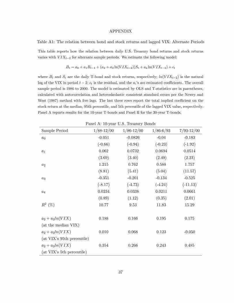
We note that the estimated a4 coefficients for this model are all positive but statistically in-
significant. In the Appendix, we report on estimating a similar model over four alternate periods.
The estimated a4’s are positive in all four periods and positive and statistically significant in the
July 1993 through December 2000 subperiod. Thus, while the statistical reliability is suspect, at
least the sign of these coefficients is consistent with the idea that bond prices may increase, relative
to stocks, during times of high stock market uncertainty.
The results in Tables 2 and 3 also imply something about the diversification value from holding
both stocks and bonds. Our findings suggest that, during times of high uncertainty in the stock
market, the relation between stock and bond returns appears much weaker. Further, the lagged
VIX is not reliably related to time-varying bond volatility (note that the estimated γ3 coefficients
are statistically insignificant in the full model of Table 3). These characteristics suggest an increased
diversification benefit from holding bonds with stocks, exactly during the times when diversification
is most needed. In contrast, several papers have suggested that cross-market equity returns become
more correlated during times of market shocks or economic uncertainty.6
4.4 Robustness: Returns from Treasury bond futures prices
We also examine the T-bond futures-return series for robustness. The futures series behaves sim-
ilarly to the 30-year bond-return series from the Federal Reserve data. The correlation between
the daily futures-return series and the 30-year bond-return series is 0.955 over the 1988 to 2000
period. Further, the volatility is comparable with the futures-return series having a daily standard
deviation of 0.568% per day versus 0.633% per day for the 30-year bond series in Table 1. The6For example, King and Wadhwani (1990) and Lee and Kim (1993) suggest that the cross-market equity correlation
increased following the U.S. market crash of 1987. However, note that Forbes and Rigobon(2001) cast some doubt
on these findings.
14

correlation between the futures-return series and the stock market return is 0.270, similar to the
0.250 correlation between the stock return and our 30-year bond-return series. Finally, we find
that the results from estimating the system in (5) and (6) with the bond-futures returns are very
similar to the results for the 30-year bond returns.
5 Variation in bond and stock return co-movements:
A regime-shifting approach
5.1 Background and motivation
The results from the previous section support the notion that stock market uncertainty (measured
by the lagged implied volatility from equity index options) is associated with substantial variation
in the dynamic relation between stock and bond returns. In this section, we extend our analysis
in a second dimension. We examine whether the regime-switching framework of Hamilton (1989)
might be useful in characterizing the dynamic relation between bond returns and stock returns.7
Accordingly, in this section, we investigate whether regime-switching behavior is exhibited in:
(1) the relation between daily T-bond and stock returns, and (2) the average T-bond returns,
relative to stock returns. If so, we are also interested in whether the regimes are associated with
variation in VIX. Our model allows the transition probabilities to be a function of the lagged VIX.
We evaluate a regime-shifting approach for the following reasons. First, as previously discussed,
prior literature suggests that this approach may prove useful. Second, in our view, the time-
series behavior of the VIX suggests that a regime-switching approach may be worthwhile. See
the upper time-series in Figure 1. Casual inspection of the VIX series suggests several regions of
distinctly different behavior. First, from 1/88 to about 9/89, the VIX decreases and then levels off
following the October 1987 crash. From around 10/89 to about 10/92, the VIX exhibits substantial
variation with several periods of high implied volatility. Then, from around 11/92 to about 2/96,7See Hamilton (1994), Chapter 22, for a review of regime-switching processes and related literature. Boudoukh,
Richardson, Smith, and Whitelaw (1999) argue that regime shifts are useful in understanding bond returns. Hamilton
and Susmel (1994) and Whitelaw (2000) study regime shifts in stock volatility. See also Hamilton and Lin (1996)
and Veronesi (1999) and (2001).
15

the VIX is lower and exhibits relatively low variability. Next, from 3/96 through 9/97 the VIX
increases modestly. Finally, from 10/97 through 2000, the VIX tends to be high with very high
variability. While any such description has some subjectivity, the regions of different VIX behavior
suggest possible regime-shifting behavior related to variation in stock market uncertainty. Third, a
regime-shifting approach is evaluated because it does not constrain the stock-bond return relation
to be related to the lagged VIX in a continuous parametric function, such as in our model (5).
Thus, a regime-shifting approach seems closer to the intuition of an occasional decoupling in stock
and bond returns during periods of economic uncertainty or market distress, as suggested by the
aforementioned Wall Street Journal articles.
5.2 The regime-switching model and results
We estimate the following two-state regime-switching model, specified as follows:
Bt = as0 + a1Bt−1 + as
2St + εt, (7)
where εt is a Gaussian innovation, s can be regarded as an unobserved state variable that follows
a two-state, first-order Markov process, and the other terms are as defined for equation (5). The
transition probability matrix is expressed as follows:
X =
p 1 − p
1 − q q
(8)
where p = Pr(st = 0|st−1 = 0; It−1), and q = Pr(st = 1|st−1 = 1; It−1). It−1 is the information set.
In stead of letting p and q be constants as is the case of Hamilton (1989), we choose to let
these transition probabilites be time-varying. Following Diebold et al. (1994), the time-varying
transition probabilities are specified as follows:
p(st = j|st−1 = j; It−1) =ecj+dj ln(V IXt−1)
1 + ecj+dj ln(V IXt−1), j = 0, 1. (9)
Thus, the transition probabilities are allowed to change with the lagged VIX levels. Hence this
model specification is flexible and encompasses a constant transition probabilities model.
16

We elect not to model heteroskedasticity in the bond returns for parsimony and the following
additional reasons. First, time-variation in bond return volatility is much smaller than time-
variation in stock return volatility. Further, the correlation between time-varying stock volatility
and time-varying bond volatility is modest and the lagged VIX is not reliably related to time-
varying bond volatility. See our prior discussion in Sections 3.2, 4.1, and 4.3, and results in Tables
2 and 3.
Our results for this regime-shifting estimation are reported in Table 4. Column one in Table
4 reports results for the 10-year Treasury bonds over the 1988 to 2000 period. In the first regime
(denoted regime-zero in the table), we find that the a02 coefficient on stock returns is large and
statistically significant at a value of 0.343. The estimated intercept, a00, is negative but insignificant.
In contrast, in the second regime (denoted regime-one in the table), we find that the a12 coefficient
on stock returns is negative and statistically significant at a value of -0.061 (a difference of 0.40,
as compared to regime-zero). For regime-one, the estimated intercept, a10, is positive and highly
statistically significant.
The results for the 30-year T-bonds are qualitatively similar but even stronger in magnitude. For
the 30-year T-bonds, the difference between a02 for regime-zero and a1
2 for regime-one is 0.62. The
estimated intercept increases from -0.0303 in regime-zero to a highly reliable 0.0924 in regime-one.
For the transition probabilities, we note the following. First, we note that the estimated c0’s are
sizeable and significantly positive. More interestingly, the estimates of d0 are significantly negative,
which indicates that an increase in V IXt−1 will lower the probability of staying in regime zero.
Hence, regime zero is associated with periods of relatively lower stock market volatilities.
This concept is illustrated by the expected durations reported in the last four rows of Table 4.
At a V IXt−1 of 15%, the expected duration of staying in regime-zero is 53.1 days for the 10-year
bond returns and 67.3 days for the 30-year bonds. In contrast, at a V IXt−1 of 30%, the expected
duration of staying in regime-zero is only 15.6 days for the 10-year bond returns and 10.0 days for
the 30-year bonds.8
For regime-one, we find that the estimated c1’s are much smaller (and statistically insignificant),8The expected duration of regime i is calculated as follows: E(D) = 1
1−pii, pii ≡ Pr(st = i|st−1 = i).
17

as compared to the c0’s. Next, in contrast to the negative d0’s, the estimated d1’s are positive
(but statistically insignificant). These point estimates for c1 and d1 imply the following expected
durations for regime-one. At a V IXt−1 of 15%, the expected duration of staying in regime-one is
only 12.7 days for the 10-year bond returns and 13.9 days for the 30-year bonds. In contrast, at a
V IXt−1 of 30%, the expected duration of staying in regime-zero is 34.4 days for the 10-year bond
returns and 19.1 days for the 30-year bonds.
Next, we further describe each regime. For the purposes of this description, we categorize an
observation as regime-zero if there is an 80% chance or greater that the observation is in regime-
zero. Likewise, we categorize an observation as regime-one if there is an 80% chance or greater that
the observation falls in regime-one.
Under this classification convention, 53.6% (54.7%) of the daily observations are categorized
as regime-zero for the 10-year bond model (30-year bond model). On the other hand, 20.6%
(18.6%)of the daily observations are categorized as regime-one for the 10-year bond model (30-year
bond model). Thus, about 25% of the observations are not clearly classified into either regime.
Next, using this classification convention, we calculate basic descriptive statistics for the return
observations in each regime. First, as suggested by the negative d0 coefficient, we note that regime-
zero has a lower stock volatility with a stock return standard deviation of only about 0.7%/day.
In contrast, for the regime-one observations, the standard deviation of stock returns is about
1.4%/day. The volatility of the bond returns varies little across the two regimes. For both the
10-year and 30-year bond returns, the bond return volatility in each regime is within 10% of the
series’ unconditional volatility.
Next, we contrast Sharpe ratios for the stock and bond returns across the two regimes. For
regime-zero in the 10-year (30-year) bond model, the daily Sharpe ratio is 0.087 (0.082) for the stock
returns and -0.032 (-0.021) for the bond returns. In contrast, for regime-one in the 10-year (30-year)
bond model, this ratio is 0.001 (0.009) for the stock returns and 0.104 (0.174) for the bond returns.
Thus, in regime-zero, stocks are less volatile, stocks substantially outperform bonds (in a Sharpe
ratio sense), and stock and bond returns exhibit a substantial positive co-movement relation. In
contrast, in regime-one, stocks are highly volatile, bonds substantially outperform stocks, and stock
18

and bond returns exhibit a reliable negative co-movement relation. These characteristics suggests
the intuition of referring to regime-zero as a ’low stock market uncertainty’ regime, and referring
to regime-one as a ’high stock market uncertainty’ regime.
For comparison, we have also estimated a version of the model that assumes constant transition
probabilities (restricts the dj ’s=0). For this variation of the model, the estimated as0’s and as
2’s
remain very similar to those shown in Table 4. The regime movements display similar characteristics
but the expected durations are somewhat longer for each regime. For example, for the 30-year bond
returns in the constant transition probability model, the expected duration is 65.8 days for regime-
zero and 28.9 days for regime-one. We perform a likelihood ratio test that compares the constant
transition probability model to our time-varying transition probability model in (7) and (8). This
test rejects the constant transition probability model with a p-value of less than 0.001 for the
10-year bond and a p-value of 0.053 for the 30-year bond.
5.3 Regime-switching and the VIX series
The results from estimating the regime-shifting model of (7) and (8) indicate that the VIX is a
statistically significant explanatory variable when modelling the transition probabilities, at least
for regime-zero. We next present the relation between VIX movements and the regimes graphically.
In Figure 1, the upper series is the VIX and the lower series is the smoothed probability of being
in regime-one for the 10-year T-bond returns. In the 1988 to 2000 period, regime-zero is the
predominant regime from about 3/88 to 8/89 and from 3/93 to 9/97. These time periods tend to
be either decreasing or low VIX periods with relatively less day-to-day variation in VIX.
In contrast, regime-one spans much of the 1/88 to 2/88, 9/89 to 2/93 and 10/97 to 12/00
periods, with occasional regime-zero interim periods. Overall, regime-one seems to be associated
with a high VIX and/or substantial day-to-day variability in VIX.
Figure 2 presents the same comparison for the regime behavior for the 30-year Treasury bond
return series. The results are comparable to those for the 10-year bond, as described in the preceding
paragraph.9
9In our previous discussion and in Figures 1 and 2, we focus on the smoothed probabilities for the regime move-
19

Eyeball statistics from Figures 1 and 2 suggest that there exists a relation between the regime
probabilities and the VIX series. To further illustrate this relation, Figure 3 shows the scatterplot of
the regime-one probability against the VIX level. This figure indicates that the specific functional
form of this relation is hard to capture parametrically. Hence, we resort to nonparametric estimation
techniques to fit the relation for the illustration in Figure 3. We use a method called “local
polynomial fitting”.10 The solid line is a fitted curve estimated nonparametrically using local
polynomial fitting with degree 1. Note that the curve is strongly upward-sloping, clearly illustrating
the association between regime-one and higher stock market uncertainty.
5.4 Comparison of inflation and short-term interest rates across the two regimes
Campbell and Ammer (1993) consider fundamental factors that may jointly determine movements
in stock and bond returns. They note that movements in real interest rates should induce a
positive correlation between stock and bond returns. On the other hand, movements in inflation
should induce a negative correlation between stock and bond returns. Thus, time-variation in the
movements in real rates and inflation might conceivably induce regime-shifts in the co-movement
between stock and bond returns.
In this subsection, we describe monthly movements in inflation and real short-term interest rates
across the regimes. For this exercise, we smooth the regime movements and categorize months from
1/88 to 2/88, 10/89 to 2/93, and 10/97 to 12/00, as predominantly regime-one months. All of the
other months are categorized as predominantly regime-zero. For inflation, we evaluate monthly
changes in the seasonally-adjusted Consumer Price Index. For the monthly short-term real interest
rate, we use the difference between the yield on 3-month T-bills and the month’s inflation.
First, we report the inflation comparison. For the entire thirteen year sample, the average
ments. The results for the filtered probabilities are similar but somewhat more noisy.10The basic idea of local polynomial fitting is very simple: in a neighborhood of an observation, say x0, a polynomial
of degree p is fitted to the data. Compared with other popular nonparametric smoothing techniques, especially kernel
regression, local polynomial fitting is known to have better small sample properties, see e.g., Fan and Gijbels (1996).
In fact, the classical Nadaraya-Waston kernel regression corresponds to the special case of a local polynomial regression
with degree zero.
20

inflation was 0.264% per month and the average absolute change in the month-to-month inflation
rate was 0.146%. For the predominantly regime-zero months, the average inflation was 0.273% per
month and the average absolute change in the month-to-month inflation rate was 0.123%. For the
predominantly regime-one months, the average inflation was 0.255% per month and the average
absolute change in the month-to-month inflation rate was 0.167%.
Next, we report the short-term interest rate comparison. For the entire thirteen year sample,
the average real rate was 0.193% per month and the average absolute month-to-month change
in the monthly T-bill yield was 0.0129% per month. For the predominantly regime-zero months,
the average real rate was 0.161% per month and the average absolute month-to-month change in
the monthly T-bill yield was 0.0134% per month. For the predominantly regime-one months, the
average real rate was 0.223% per month and the average absolute month-to-month change in the
monthly T-bill yield was 0.0126% per month.
Based on these cross-regime comparisons, it seems unlikely that the regime-shifting behavior is
attributable to differences in the behavior of inflation or the short-term discount rate across the two
regimes. Indirectly, this finding seems to support the idea that stock market uncertainty influences
cross-market return dynamics.
5.5 Discussion of results
Our collective results suggest that implied equity volatility may serve as a state variable for un-
derstanding variations in the stock-bond return relation. Our evidence suggest that stock and
bond returns tend to move together substantially during periods of lower stock market uncertainty.
However, higher stock market uncertainty is associated with little co-movement or even a negative
co-movement between stock and bond returns.
For our regime-shifting model, it is perhaps puzzling that the negative relation between stock
and bond returns is exhibited over a sustained period during regime-one. This finding seems at
odds with a simple flight-to-quality interpretation that assumes that stock and bond prices move
in the opposite direction only briefly during the period when stock uncertainty increases. Rather,
our findings suggest that there may be sustained periods of negative correlation between stock
21

and bond returns, possibly because investors may be frequently revising their estimates about
the economic state during times of higher uncertainty. This notion seems consistent with the
intuition from Veronesi (1999 and 2001) and the second Wall Street Journal article mentioned in
our introduction.
In our view, since the expected duration of regime-one is typically only in the 10 to 20 day
range, regime-one may be interpreted as a transitional state associated with higher stock market
uncertainty. In contrast, the expected duration of regime-zero is much larger at 50 to 60 days (for
typical level of VIX). Thus, regime-zero may be interpreted as more normal times, where stock and
bond returns may be linked primarily by common fundamentals.
6 Bond returns and changes in stock implied volatility
So far, we have examined whether the contemporaneous relation between stock and bond returns
varies with stock market uncertainty, where stock market uncertainty is measured by the lagged
V IX level. Here, we report on a different aspect of stock and bond return dynamics to supplement
our primary findings.
It is known that stock returns are negatively and reliably associated with contemporaneous
changes in VIX (ρS,DV IX = −0.71 in our sample), see Fleming, Kirby, and Ostdiek (1995). However,
it is not known whether bond returns are related to changes in VIX, after controlling for the period’s
stock return. To examine this issue, we estimate the following GARCH(1,1) model to examine the
relation between bond returns, stock returns, and contemporaneous changes in VIX.
Bt = α0 + α1Bt−1 + α2St + α3DV IXt + εt, (10)
ht = γ0 + γ1ε2t−1 + γ2h
2t−1. (11)
where Bt denotes the T-bond return in period t, St is the contemporaneous stock return, DV IXt
is the change in the implied variance from the CBOE’s VIX between the end of period t − 1 and
the end of period t, εt is the residual, ht denotes the conditional variance, and the αi’s and γi’s are
estimated coefficients. The above system is estimated simultaneously by maximum likelihood with
22

the conditional normal density. We report t-statistics calculated with quasi-maximum likelihood
(QML) standard errors in accordance with Bollerslev and Wooldridge, 1992.
The coefficient of primary interest is α3. If positive, it suggests that bond prices tend to increase,
relative to stocks, during days when the stock market uncertainty increases. The model is estimated
for both the 10-year and 30-year Treasury bonds.
Table 5 reports the results. For both the 10-year and 30-year T-bond returns, the estimated
coefficients for DVIX (α3) are significantly positive. We conclude that T-bond returns are positively
and reliably associated with changes in VIX, after controlling for the stock return. This finding
seems consistent with the idea of cross-market hedging (or flight-to-quality) during periods when
stock market uncertainty increases.
7 Conclusion
We examine how the co-movement between daily stock and Treasury bond returns varies with stock
market uncertainty. We use the lagged implied volatility from equity index options (the CBOE’s
VIX) to provide an objective, observable, and dynamic measure of stock market uncertainty. We
find that stock and bond returns tend to move substantially together during periods of lower stock
market uncertainty. However, stock and bond returns tend to exhibit little relation or even a
negative relation during periods of high stock market uncertainty.
We find evidence of these return dynamics in the following alternate approaches in examining
the data: (1) a simple correlation analysis, (2) a GARCH specification that allows the relation
between stock and bonds to vary directly and continuously with the lagged VIX, and (3) a regime-
shifting model that allows the relation between stocks and bonds to vary across regimes. The
regime-shifting model also indicates that average bond returns are relatively higher in the regime
with a negative co-movement between daily stock and bond returns. In contrast, average stock
returns are relatively higher in the regime with a high positive co-movement between daily stock
and bond returns.
Finally, after controlling for the period’s stock return, we find a reliable positive relation between
daily bond returns and the contemporaneous change in VIX. This finding is in contrast to the very
23

large negative relation between stock returns and contemporaneous changes in VIX.
Our findings have implications for understanding the joint price formation process for stocks
and bonds. First, as suggested in Fleming, Kirby, and Ostdiek (1998), our results are consistent
with the notion that cross-market hedging may generate time-varying demand for bonds and an
associated influence on the joint return dynamics between stocks and bonds.
Next, our results might be interpreted from the framework of intertemporal asset-pricing. If
implied volatility is interpreted as a state variable that is informative about the investment op-
portunity set or about economic uncertainty (in the sense of Veronesi, 1999 and 2001), then this
might explain the link between stock market uncertainty and the time-varying co-movement be-
tween stock and bond returns. For example, if the relative attractiveness of bonds versus stocks is
volatile during periods of stock market uncertainty, then sustained periods of negative correlation
between stocks and bond returns may be observed. In our view, such potential explanations do
not replace a cross-market hedging perspective, but rather supplements it. Future research on the
economics behind our findings might prove interesting.
Third, our findings imply that models that jointly examine stock and bond returns should allow
for the stock-bond return relation to vary with expected stock volatility. In contrast, previous
bivariate GARCH models for stock and bond returns has generally assumed a constant correlation
between return series (see, e.g. Scruggs (1998)).
From a practical perspective, our results may have direct financial applications. Specifically,
implied stock volatility may be a useful state variable for financial applications that need to un-
derstand and predict stock and bond market co-movements. For example, our findings suggest
increased diversification benefits for portfolios of stocks and bonds during periods of high stock
market uncertainty. Such a timely diversification benefit is in contrast to cross-equity market di-
versification, where much of the literature has argued that cross-market equity returns may be more
positively linked during times of high stock market uncertainty.
24

References
Bakshi, Gurdip, & Nikunj Kapadia, 2001, Delta-hedged gains and the negative market volatility
risk premium, The Review of Financial Studies forthcoming.
Barsky, R, 1989, Why don’t the prices of stocks and bonds move together?, American Economic
Review 79, 1132–1145.
Blair, Bevan, Ser-Huang Poon, & Stephen Taylor, 2001, Forecasting S&P 100 volatility: The incre-
mental information content of implied volatilities and high-frequency index returns, Journal
of Econometrics 105, 5–26.
Bollerslev, Tim, & Jeffrey M. Wooldridge, 1992, Quasi-maximum likelihood estimation inference
in dynamic models with time-varying covariances, Econometric Theory 11, 143–172.
Boudoukh, Jocob, Matthew Richardson, Tom Smith, & Robert Whitelaw, 1999, Regime shifts and
bond returns, Working Paper, New York University.
Campbell, John Y., & John Ammer, 1993, What moves the stock and bond markets? A variance
decomposition for long-term asset returns, The Journal of Finance 48, 3–37.
Campbell, John Y., Martin Lettau, Burton G. Malkiel, & Yexiao Xu, 2001, Have individual stocks
become more volatile? An empirical exploration of idiosyncratic risk, The Journal of Finance
56, 1–43.
Christensen, B. J., & N. R. Prabhala, 1998, The relation between implied and realized volatility,
Journal of Financial Economics 50, 125–150.
Coval, Joshua, & Tyler Shumway, 2001, Expected option returns, The Journal of Finance 56,
983–1009.
David, Alexander, & Pietro Veronesi, 2000, Option prices with uncertain fundamentals: Theory
and evidence on the dynamics of implied volatilities, Working Paper, University of Chicago.
25

Diebold, F. X., J. H. Lee, & G. C. Weinbach, 1994, Regime switching with time-varying transi-
tion probabilities, in C. Hargreaves, (ed.) Time Series Analysis and Cointegration (Oxford
University Press).
Fama, Eugene F., & Kenneth R. French, 1989, Business conditions and expected returns on stocks
and bonds, Journal of Financial Economics 25, 23–49.
Fan, J., & I. Gijbels, 1996, Local Polynomial Modelling and Its Applications (Chapman & Hall,
UK).
Fleming, Jeff, Chris Kirby, & Babara Ostdiek, 2001, The economic value of volatility timing, The
Journal of Finance 56, 329–352.
Fleming, Jeff, Chris Kirby, & Barbara Ostdiek, 1998, Information and volatility linkages in the
stock, bond, and money markets, Journal of Financial Economics 49, 111–137.
Fleming, Jeff, Barbara Ostdiek, & R. Whaley, 1995, Predicting stock market volatility: A new
measure, Journal of Futures Market 15, 265–302.
Fleming, J., 1998, The quality of market volatility forecast implied by S&P 100 index option prices,
Journal of Empirical Finance 5, 317–345.
Fleming, M., 1997, The round-the-clock market for U.S. treasury securities, Economy Policy Review
9–32.
Forbes, Kristin, & Roberto Rigobon , 2001, No contagion, only interdependence: Measuring stock
market co-movements, The Journal of Finance forthcoming.
Hamilton, James D., & Gang Lin, 1996, Stock market volatility and the business cycle, Journal of
Applied Econometrics 11, 573–593.
Hamilton, James D., & Raul Susmel, 1994, Autoregressive conditional heteroscedasticity and
changes in regime, Journal of Econometrics 64, 307–333.
Hamilton, James D., 1989, A new approach to the economic analysis of nonstationary time series
and the business cycle, Econometrica 57, 357–384.
26

Haugen, R., E. Talmor, & W. Torous, 1991, The effect of volatility changes on the level of stock
prices and subsequent expected returns, The Journal of Finance 46, 985–1007.
King, Mervyn, & Sushil Wadhwani, 1990, Transmission of volatility between stock markets, The
Review of Financial Studies 3, 5–33.
Lee, Sang, & Kwang Kim, 1993, Does the October 1987 crash strengthen the co-movements among
national stock markets?, Review of Financial Economics 3, 89–102.
Poteshman, Allen M., 2000, Forecasting future volatility from option prices, Working Paper, Uni-
versity of Illinois at Urbana-Champaign.
Schwert, William G., 1989, Why does stock market volatility change over time?, The Journal of
Finance 44, 1115–1153.
Scruggs, J., 1998, Resolving the puzzling intertemporal relation between the market risk premium
and conditional market variance: A two-factor approach, Journal of Finance 53, 575–603.
Shiller, R., & A. Beltratti, 1992, Stock prices and bond yields: Can their comovements be explained
in terms of present value models?, Journal of Monetary Economics 30, 25–46.
Veronesi, P., 1999, Stock market overreaction to bad news in good time: A rational expectations
equilibrium model, The Review of Financial Studies 12, 957–1007.
Veronesi, P., 2001, Belief-dependent utilities, aversion to state-uncertainty and asset prices, Work-
ing Paper, University of Chicago.
Whitelaw, Robert F., 1994, Time variation and covariations in the expectation and volatility of
stock market returns, The Journal of Finance 49, 515–541.
Whitelaw, Robert, 2000, Stock market risk and return: An equilibrium approach, The Review of
Financial Studies 13, 521–547.
27

Table 1: Descriptive statistics
This table reports the descriptive statistics for the data used in this article. S, B10, and
B30 refer to the stock, 10-year Treasury bond, and 30-year Treasury bond return series,
respectively. DVIX stands for the daily change in the implied variance from the Chicago
Board Option Exchange’s Volatility Index (VIX). Std. Dev. denotes standard deviation
and ρi refers to the ith autocorrelation. All of the returns are in daily percentage form.
The sample period is 1988 to 2000. Panel A reports univariate statistics for each series and
Panel B reports the correlation matrix.
Panel A: Basic Univariate Statistics
VIX DVIX S B10 B30
Mean 19.845 -0.001 0.061 0.028 0.035
Median 18.690 -0.003 0.084 0.021 0.021
Maximum 49.360 4.983 4.828 1.926 3.082
Minimum 9.040 -3.147 -6.592 -2.732 -3.805
Std. Dev. 6.293 0.322 0.892 0.414 0.633
ρ1 0.973 -0.160 0.060 0.075 0.032
ρ2 0.953 -0.102 -0.023 -0.004 0.015
ρ3 0.937 -0.055 -0.036 -0.044 -0.029
Panel B: Correlations
VIX DVIX S B10 B30
VIX 1.000
DVIX 0.104 1.000
S -0.136 -0.712 1.000
B10 -0.025 -0.056 0.219 1.000
B30 -0.029 -0.089 0.250 0.936 1.000
28

Table 2: The correlation between stock and bond returns, conditional on V IXt−1
This table reports the correlation between stock and bond returns for different subsets of
return observations. The sample is stratified into quintiles by sorting on V IXt−1. S, B10,
and B30 refer to the stock, 10-year Treasury bond, and 30-year Treasury bond return series,
respectively. ρ, µ, and σ indicate correlation, mean, and standard deviation, respectively.
Panel A reports the actual sample statistics for this sort. Panel B reports hypothetical
correlations under two alternate simple benchmarks. Benchmark One assumes that the
expected bond return, given the stock return, can be expressed as a constant times the stock
return. Benchmark Two assumes that the expected stock return, given the bond return,
can be expressed as a constant times the bond return. See Section 4.2 for the complete
statistical assumptions and calculation method for these hypothetical correlations.
Panel A: Sample statistics of the V IXt−1 quintiles
VIX quintile Low 2nd 3rd 4th High
ρS,B10 0.443 0.318 0.428 0.283 0.015
ρS,B30 0.472 0.365 0.411 0.300 0.078
µS 0.061 0.033 0.084 0.079 0.049
σS 0.488 0.657 0.676 0.926 1.41
µB10 0.038 0.028 0.020 0.026 0.029
σB10 0.405 0.411 0.408 0.391 0.453
µB30 0.049 0.036 0.017 0.033 0.039
σB30 0.611 0.592 0.607 0.638 0.711
Panel B: Hypothetical correlations under simple benchmarks
VIX quintile Low 2nd 3rd 4th High
Benchmark One: ρS,B10 0.153 0.203 0.210 0.300 0.396
Benchmark Two: ρS,B10 0.388 0.293 0.283 0.198 0.150
29

Table 3: The relation between bond returns and stock returns as a function of lagged VIX
This table reports how the relation between daily U.S. Treasury bond returns and stock returnsvaries with the lagged VIX level. We estimate the following GARCH model:
Bt = a0 + a1Bt−1 + (a2 + a3 ln(V IXt−k))St + a4 ln(V IXt−k) + εt
ht = γ0 + γ1ε2t−1 + γ2ht−1 + γ3V IXt−2
where Bt and St are the daily T-bond and stock returns, respectively; V IXt−k is the CBOE’sVolatility Index in period t−k; εt is the residual, ht is the conditional variance, and the ai’s and γi’sare estimated coefficients. T-statistics are in parentheses, calculated with quasi-maximum likelihoodstandard errors in accordance with Bollerslev and Wooldridge (1992). The sample period is 1988to 2000. The last three rows report the total implied coefficient on the stock return at the median,95th percentile, and 5th percentile of the lagged VIX value, respectively.
Panel A: 10-Year U.S. Treasury BondsBase k = 2 k = 22
a0 0.019 -0.032 -0.046(2.91) (-0.53) (-0.64)
a1 0.074 0.066 0.072(6.18) (4.44) (5.39)
a2 0.127 1.20 1.14(10.6) (12.2) (6.76)
a3 -0.347 -0.330(-11.6) (-6.03)
a4 0.017 0.0217(0.83) (0.89)
γ0 0.0265 0.0093 0.011(9.59) (2.11) (2.30)
γ1 0.067 0.034 0.040(4.45) (3.85) (4.16)
γ2 0.735 0.891 0.867(154.5) (21.3) (18.4)
γ3 0.0034 0.0012 0.0017(2.66) (1.21) (1.27)
Likel. Function 1372.2 1463.5 1443.1
a2 + a3ln(V IX) 0.188 0.173(at the median VIX)a2 + a3ln(V IX) 0.012 0.006(at VIX’s 95th percentile)a2 + a3ln(V IX) 0.352 0.329(at VIX’s 5th percentile)
30

Table 3: (continued)
Panel B: 30-Year U.S. Treasury BondsBase k = 2 k=22
a0 0.022 -0.048 -0.073(1.76) (-0.45) (-0.71)
a1 0.011 0.018 0.022(0.69) (1.11) (1.46)
a2 0.228 1.88 1.85(9.75) (9.00) (7.81)
a3 -0.534 -0.531(-8.17) (-6.98)
a4 0.023 0.031(0.63) (0.90)
γ0 0.019 0.028 0.047(0.32) (0.68) (1.08)
γ1 0.029 0.027 0.0312(2.14) (3.12) (2.83)
γ2 0.889 0.860 0.769(4.88) (4.94) (4.21)
γ3 0.0058 0.0071 0.0139(0.47) (0.61) (0.94)
Likel. Function 20.29 105.55 87.47
a2 + a3ln(V IX) 0.314 0.292(at the median VIX)a2 + a3ln(V IX) 0.044 0.023(at VIX’s 95th percentile)a2 + a3ln(V IX) 0.567 0.544(at VIX’s 5th percentile)
31

Table 4: A regime-shifting model for the relation between stock and bond returns
This table reports the results for the following regime-switching model.
Bt = as0 + a1Bt−1 + as
2St + εt,
where the regime variable st has time-varying transition probabilities:
p(st = j|st−1 = j; It−1) =ecj+dj ln(V IXt−1)
1 + ecj+dj ln(V IXt−1), j = 0, 1.
where It−1 is the information set at t − 1, the cj ’s and dj ’s are estimated coefficients, andthe other terms are as defined in Table 3. The sample period is 1988 to 2000. T-statisticsare in parentheses. The final rows give the expected duration of each regime for differentV IXt−1 levels.
10-yr T-Bonds 30-yr T-Bondsa0
0 -0.0156 (-1.51) -0.0303 (-1.92)
a10 0.0558 (4.26) 0.0924 (4.28)
a1 0.0577 (3.63) 0.0102 (0.642)
a02 0.3430 (14.7) 0.5297 (13.8)
a12 -0.0609 (-4.99) -0.0930 (-4.54)
c0 8.9163 (2.93) 11.9900 (3.83)
d0 -1.8327 (-1.86) -2.8789 (-2.97)
c1 -1.6240 (-0.55) 1.2433 (0.42)
d1 1.5090 (1.59) 0.4853 (0.53)
Expected Duration(st = 0, V IXt−1 = 15%) 53.1 days 67.3 days(st = 0, V IXt−1 = 30%) 15.6 days 10.0 days(st = 1, V IXt−1 = 15%) 12.7 days 13.9 days(st = 1, V IXt−1 = 30%) 34.4 days 19.1 days
32

Table 5: Bond returns and contemporaneous changes in stock implied volatility
This table reports how daily U.S. Treasury bond returns are jointly related to the day’sstock returns and the daily change in the VIX level.
Bt = α0 + α1Bt−1 + α2St + α3DV IXt + εt
ht = γ0 + γ1ε2t−1 + γ2ht−1 + γ3V IXt−1
where DV IXt is the change in the implied variance from the CBOE’s VIX between the endof day t− 1 and the end of day t, the αi’s and γi’s are estimated coefficients, and the otherterms are as defined in Table 3. The sample period is 1988 to 2000. T-statistics are inparentheses, calculated with quasi-maximum likelihood standard errors in accordance withBollerslev and Wooldridge (1992).
10-yr T-Bonds 30-yr T-Bondsα0 0.018 0.0204
(3.04) (1.94)
α1 0.060 0.0136(4.28) (1.03)
α2 0.183 0.305(13.3) (13.0)
α3 0.250 0.354(4.60) (3.88)
γ0 0.0056 0.0094(2.66) (2.21)
γ1 0.036 0.028(4.55) (4.60)
γ2 0.921 0.934(43.4) (42.80)
γ3 0.0007 0.0026(1.20) (1.50)
33

Figure 1
This figure displays the CBOE’s Volatility Index (upper series) and the smooth probability of beingin regime-one (lower series) from the regime-shifting model in Table 4 for the 10-year Treasury bondreturns. The sample period is 1988 to 2000.
0
0.2
0.4
0.6
0.8
1
1.2
1.4
1.6
1.8
2
2.2
2.4
2.6
Jan-
88
May
-88
Oct
-88
Mar
-89
Aug
-89
Jan-
90
May
-90
Oct
-90
Mar
-91
Aug
-91
Jan-
92
May
-92
Oct
-92
Mar
-93
Aug
-93
Jan-
94
May
-94
Oct
-94
Mar
-95
Aug
-95
Jan-
96
May
-96
Oct
-96
Mar
-97
Aug
-97
Jan-
98
May
-98
Oct
-98
Mar
-99
Aug
-99
Jan-
00
May
-00
Oct
-00
DATE (month/year)
RE
GIM
E-O
NE
PR
OB
AB
ILIT
Y
-20
-10
0
10
20
30
40
50
VIX
34

Figure 2
This figure displays the CBOE’s Volatility Index (upper series) and the smooth probability of beingin regime-one (lower series) from the regime-shifting model in Table 4 for the 30-year Treasury bondreturns. The sample period is 1988 to 2000.
0
0.2
0.4
0.6
0.8
1
1.2
1.4
1.6
1.8
2
2.2
2.4
2.6
Jan-
88
May
-88
Oct
-88
Mar
-89
Aug
-89
Jan-
90
May
-90
Oct
-90
Mar
-91
Aug
-91
Jan-
92
May
-92
Oct
-92
Mar
-93
Aug
-93
Jan-
94
May
-94
Oct
-94
Mar
-95
Aug
-95
Jan-
96
May
-96
Oct
-96
Mar
-97
Aug
-97
Jan-
98
May
-98
Oct
-98
Mar
-99
Aug
-99
Jan-
00
May
-00
Oct
-00
DATE (month/year)
RE
GIM
E-O
NE
PR
OB
AB
ILIT
Y
-20
-10
0
10
20
30
40
50
VIX
35

Figure 3
This figure plots the regime-one probability of 10-year T-bond against log (VIX). The solid line isestimated nonparametrically using local polynomial fitting. The sample period is 1988 to 2000.
2.5 3.0 3.5
0.0
0.2
0.4
0.6
0.8
1.0
log(VIX)
Pro
babi
lity
36
APPENDIX
Table A1: The relation between bond and stock returns and lagged VIX: Alternate Periods
This table reports how the relation between daily U.S. Treasury bond returns and stock returns
varies with V IXt−2 for alternate sample periods. We estimate the following model:
Bt = a0 + a1Bt−1 + (a2 + a3 ln(V IXt−2))St + a4 ln(V IXt−2) + εt
where Bt and St are the daily T-bond and stock returns, respectively; ln(V IXt−2) is the natural
log of the VIX in period t− 2; εt is the residual, and the ai’s are estimated coefficients. The overall
sample period is 1986 to 2000. The model is estimated by OLS and T-statistics are in parentheses,
calculated with autocorrelation and heteroskedastic consistent standard errors per the Newey and
West (1987) method with five lags. The last three rows report the total implied coefficient on the
stock return at the median, 95th percentile, and 5th percentile of the lagged VIX value, respectively.
Panel A reports results for the 10-year T-bonds and Panel B for the 30-year T-bonds.
Panel A: 10-year U.S. Treasury Bonds
Sample Period 1/88-12/00 1/86-12/00 1/86-6/93 7/93-12/00
a0 -0.051 -0.0826 -0.04 -0.183
(-0.66) (-0.94) (-0.23) (-1.92)
a1 0.062 0.0732 0.0694 0.0514
(3.69) (3.40) (2.49) (2.23)
a2 1.215 0.762 0.588 1.757
(8.81) (5.41) (5.04) (11.57)
a3 -0.351 -0.201 -0.134 -0.525
(-8.17) (-4.73) (-4.24) (-11.13)
a4 0.0234 0.0338 0.0211 0.0661
(0.89) (1.12) (0.35) (2.01)
R2 (%) 10.77 9.53 11.83 15.29
a2 + a3ln(V IX) 0.188 0.166 0.195 0.175
(at the median VIX)
a2 + a3ln(V IX) 0.010 0.068 0.123 -0.050
(at VIX’s 95th percentile)
a2 + a3ln(V IX) 0.354 0.266 0.243 0.485
(at VIX’s 5th percentile)
37

Table A1: (continued)
Panel B: 30-Year U.S. Treasury BondsSample Period 1/88-12/00 1/86-12/00 1/86-6/93 7/93-12/00a0 -0.089 -0.147 -0.125 -0.27
(-0.77) (-1.11) (-0.48) (-1.92)a1 0.017 0.0415 0.047 0.01
(1.02) (2.12) (1.92) (0.43)a2 1.85 1.199 0.944 2.69
(9.14) (6.15) (5.70) (13.57)a3 -0.526 -0.312 -0.213 -0.796
(-8.31) (-5.29) (-4.67) (-13.09)a4 0.037 0.056 0.050 0.097
(0.93) (1.23) (0.56) (1.99)R2 (%) 11.66 10.75 13.8 15.33
a2 + a3ln(V IX) 0.309 0.274 0.319 0.288(at the median VIX)a2 + a3ln(V IX) 0.042 0.123 0.204 -0.052(at VIX’s 95th percentile)a2 + a3ln(V IX) 0.558 0.430 0.394 0.758(at VIX’s 5th percentile)
38