NBER WORKING PAPER SERIES

STOCK VOLATILITY DURING THE RECENT FINANCIAL CRISIS

G. William Schwert

Working Paper 16976http://www.nber.org/papers/w16976

NATIONAL BUREAU OF ECONOMIC RESEARCH1050 Massachusetts Avenue

Cambridge, MA 02138April 2011

The opinions are those of the author, not the University of Rochester or the National Bureau of EconomicResearch. This paper is based on material that was presented as the Keynote address at the EuropeanFinancial Management Association meeting in June 2010. The views expressed herein are those ofthe author and do not necessarily reflect the views of the National Bureau of Economic Research.

NBER working papers are circulated for discussion and comment purposes. They have not been peer-reviewed or been subject to the review by the NBER Board of Directors that accompanies officialNBER publications.

© 2011 by G. William Schwert. All rights reserved. Short sections of text, not to exceed two paragraphs,may be quoted without explicit permission provided that full credit, including © notice, is given tothe source.

Stock Volatility During the Recent Financial CrisisG. William SchwertNBER Working Paper No. 16976April 2011JEL No. G11,G12

ABSTRACT

This paper uses monthly returns from 1802-2010, daily returns from 1885-2010, and intraday returnsfrom 1982-2010 in the United States to show how stock volatility has changed over time. It also usesvarious measures of volatility implied by option prices to infer what the market was expecting to happenin the months following the financial crisis in late 2008. This episode was associated with historicallyhigh levels of stock market volatility, particularly among financial sector stocks, but the market didnot expect volatility to remain high for long and it did not. This is in sharp contrast to the prolongedperiods of high volatility during the Great Depression. Similar analysis of stock volatility in the UnitedKingdom and Japan reinforces the notion that the volatility seen in the 2008 crisis was relatively short-lived.While there is a link between stock volatility and real economic activity, such as unemployment rates,it can be misleading.

G. William SchwertWilliam E. Simon Graduate School of Business AdministrationUniversity of RochesterRochester, NY 14627and NBERSchwert@schwert.ssb.rochester.edu

1

"We are in the worst financial crisis since the Great Depression, and a lot of you I think are worried about your jobs, your pensions, your retirement accounts," Democratic presidential candidate Barack Obama as he opened a debate with Republican rival John McCain, October 7, 2008 (Reuters).

1. Introduction

This quote has been repeated often by President Obama since that debate, and many

commentators have called the recent recession the “Great Recession,” to reflect the size and

significance of the economic slowdown. Yet, at the time of the Obama-McCain debate, the

September 2008 unemployment rate was only 6.2 percent (up from 4.7 percent a year earlier).

Moreover, the National Bureau of Economic Research (NBER) did not announce that a recession

had started in January 2008 until December 1, 2008.

So what caused candidate Obama to relate the financial crisis of 2008 to the Great

Depression? An obvious answer is that the volatility of stock prices, particularly among financial

sector stocks, had spiked so high in the days before that debate that the entire country was noticing

and worrying about the condition of US financial markets. The implied volatility of the Standard &

Poor’s 500 portfolio, which is calculated from the prices of put and call options traded on the

Chicago Board Options Exchange (CBOE) and is referred to as the VIX index, closed at an annual

standard deviation of return of 68.01 percent on October 8, compared with just 24.72 percent on

September 8, 2008. The large swings in stock prices were the lead stories for most news

organizations, usually followed by speculation about the future economic conditions in the whole

economy. Indeed, concerns about systemic risk, the absence of liquidity, and the stability of the

financial system led to a variety of unusual measures to restore confidence in the stock and credit

markets.

2

My goal in this paper is to review the behavior of financial volatility during the 2008

financial crisis, to put it into historical context, to show how markets did not expect the high

volatility to persist for long, and to show that market expectations were accurate, since volatility

returned to more normal levels relatively quickly. Finally, I discuss the connections between stock

volatility and the real economy.

2. What Is Volatility?

2.1 Large Percentage Changes in Prices

Table 1 shows the 35 largest increases and decreases in the Dow Jones Industrial Average

(DJIA) during its history, from 1885-2010 (34,663 days). On September 29, 2008, the DJIA fell

from 11,143 to 10,365, over 777 points. This was the largest one day drop in market stock prices

since Dow Jones began computing index numbers in 1885. Less than a month later, on October 13,

2008, the DJIA rose over 936 points in one day. Not surprisingly, the popular press was focused on

these all-time records.

The academic finance profession widely agrees that volatility should be measured in

percentage changes in prices, or rates of return. If you invest $1,000 today in a portfolio of common

stocks, the rate of return tells you the proportional change in the value of your investment after the

period. A ten percent rate of return would mean an increase in value of $100 whether the DJIA was

at 100, 1,000, or 10,000.

By focusing on the absolute level of the DJIA, the press and the public exaggerate the

severity of recent volatility. For example, the Dow Jones index reached above 778 for the first time

on January 22, 1964, so it would have been impossible for the index to drop 777 points before that

date. Table 2 shows the 35 largest percentage increases and decreases in the DJIA from 1885-2010.

3

The DJIA fell by only 38 and 31 points on October 28 and 29, 1929, yet these second and third

largest daily percentage drops in the history of the New York Stock Exchange, and the October 15,

2008 drop represented only the tenth largest one day percentage drop in the history of the DJIA.

In the past I have suggested (only partly in jest) that the problem of volatility could be solved

if Dow Jones (the publisher of the Wall Street Journal) would simply do what the Bureau of Labor

Statistics does periodically with the Consumer Price Index: rescale the index equal to 100 in some

recent period. Then absolute changes in the price index would approximate percentage changes, so

the press and the public would not be fooled when the level of the index is higher than it has been in

the past.

In Table 1 I highlight October 19, 1987 because it is the only day among these 70 largest

increases and decreases that happened before 1997. In contrast, in Table 2 I highlight the 11 days

since 2001 that are among the 70 largest percentage increases or decrease in the DJIA. Several

patterns are clear from these tables. First, there are many reversals, when large drops in stock prices

have been followed by large increases in stock prices. For example, the 1929 stock market crash

represents two of the largest percentage drops in stock prices, -12.3 and -10.2 percent on October 28

and 29. The market rebounded on October 30 with the third largest one day percentage gain in the

sample, 12.5 percent. This is characteristic of an increase in stock market volatility; that is, an

increased chance of large stock returns of either sign. Most of the largest returns occurred during

the Great Depression from 1929-1939. This is a simple way to show there were high levels of stock

market volatility.

2.2 Standard Deviations of Returns

The most commonly used measure of stock return volatility is the standard deviation. This

4

statistic measures the dispersion of returns. Financial economists find the standard deviation to be

useful because it summarizes the probability of seeing extreme values of returns. When the

standard deviation is large, the chance of a large positive or negative return is large.

The tables and figures below show the historical behavior of stock volatility through several

different lenses of a microscope. At the most distant setting, we can see volatility based on monthly

returns all the way back to 1802 in the United States. If we want to look more closely at

intra-month movements in stock prices, we can use daily returns that are available since 1885.

Finally, if we want to be able to focus on intra-day movements in stock prices, we can use 15-minute

returns that are available since 1982. Each of these perspectives gives insights into the recent

episodes of high volatility, yet the overall picture that emerges is quite consistent: the 2008

financial crisis was relatively short-lived.

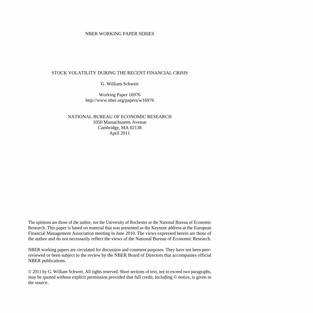
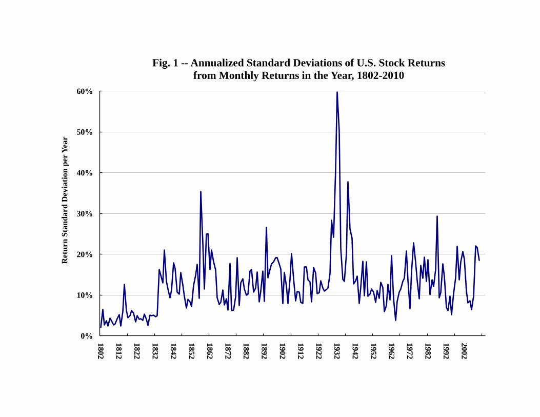
Figure 1 shows a plot of the standard deviation of monthly returns to an index of United

States stocks from 1802-2010.2 Each year the 12 monthly returns are used to calculate the standard

deviation, so there is one point per year in the plot. This plot shows that stock return standard

deviations are about 13 percent per year. Since the US stock market started to include railroad and

industrial corporations, around 1834, the volatility of returns to this aggregate stock portfolio has

been remarkably stable, with the exception of the Great Depression, from 1929-1939, when the

standard deviation was around 30 percent per year. This longer-term perspective on stock market

volatility makes it clear that the last couple of years have not been that unusual.

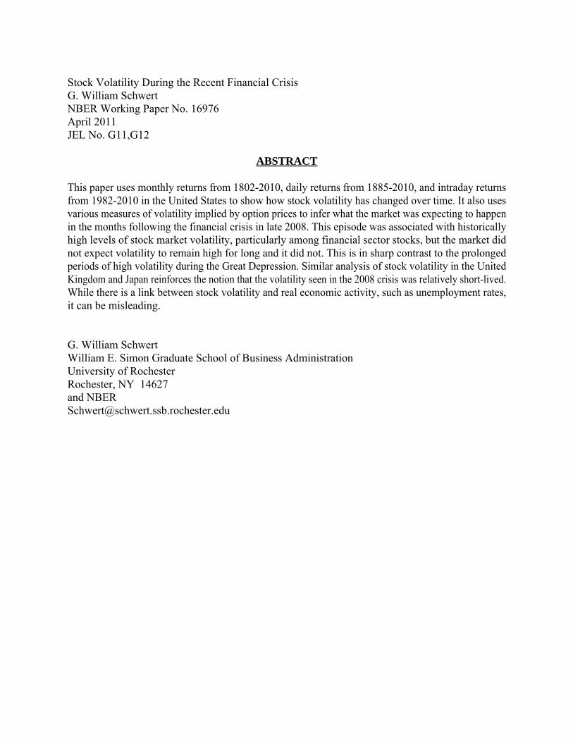
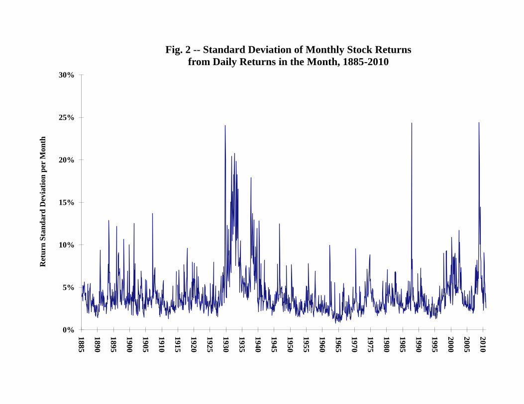
Figure 2 shows a plot of the standard deviation of monthly returns to an index of New York

2 The data from 1802-1925 are from Schwert (1990). The data from 1926-2009 are from the Center for Research in Security Prices (CRSP), representing a value-weighted portfolio of stocks from the New York and American Stock Exchanges, from NASDAQ, and from ARCA. For 2010, I use the Standard & Poor’s (S&P) 500 portfolio.

5

Stock Exchange-listed stocks from 1885-2010.3 Each month the daily returns are used to calculate

the standard deviation for the month. Since returns are not highly correlated through time, the

standard deviation of monthly returns is about equal to the standard deviation of daily returns times

the square root of the number of trading days in the month. This transformation is used in figure 2.

There are over 1,500 standard deviation estimates in figure 2, each based on about 21 trading

days per month. In contrast, figure 1 contains 209 standard deviation estimates each based on 12

months per year. Thus, figure 2 contains much more information about volatility. It is also clear

that months like October 1929, October 1987, and October 2010 show up more clearly in figure 2

because volatility was very high for brief periods of time. Otherwise, the results in figures 1 and 2

reinforce each other. The typical level of the monthly standard deviation is about 4 percent. The

standard deviation estimates are over 8 percent from September 2008 through May 2009. To put

this in perspective, though, there were 10 months between April 2000 and October 2002 that also

had standard deviations above 8 percent.

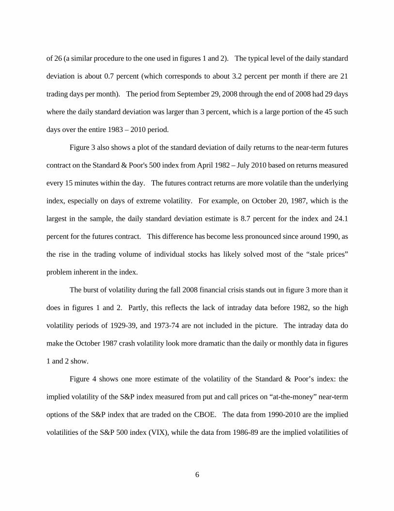
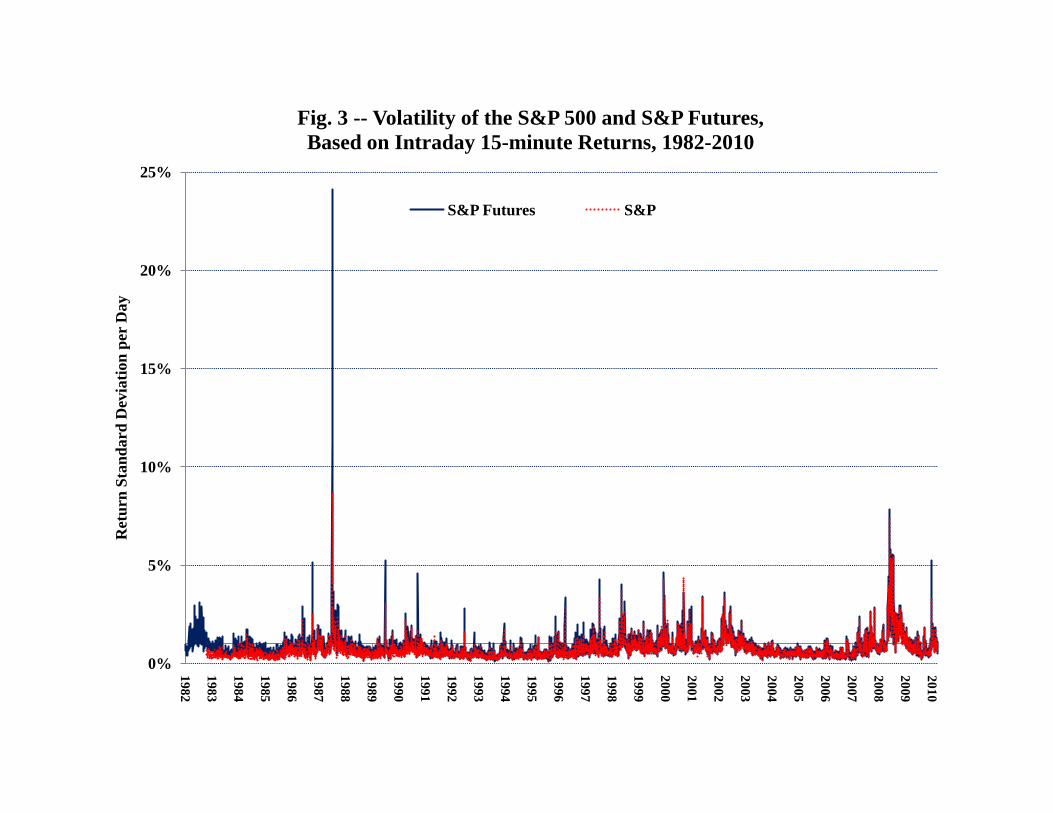
For recent years, it is possible to measure volatility using prices measured within the day.

Figure 3 shows a plot of the standard deviation of daily returns to the Standard & Poor's 500 index

from February 1983 – July 2010 based on returns measured every 15 minutes within the day.4

Thus, there are about 26 intraday returns used to calculate each daily standard deviation. To

measure the daily standard deviation, I multiply the 15 minute standard deviation by the square root

3 The data from 1802-1962 are from Schwert (1990). The data from 1962-2009 are from the Center for Research in Security Prices (CRSP), representing a value-weighted portfolio of stocks from the New York and American Stock Exchanges, from NASDAQ, and from ARCA. For 2010, I use the Standard & Poor’s (S&P) 500 portfolio. 4 The choice of a 15-minute interval for estimating the standard deviation is driven by the autocorrelation of shorter-interval intraday returns to the S&P index caused by non-synchronous trading of the stocks within the index. Returns to the futures contract, which does not have not have this problem, are not substantially autocorrelated even at one minute intervals.

6

of 26 (a similar procedure to the one used in figures 1 and 2). The typical level of the daily standard

deviation is about 0.7 percent (which corresponds to about 3.2 percent per month if there are 21

trading days per month). The period from September 29, 2008 through the end of 2008 had 29 days

where the daily standard deviation was larger than 3 percent, which is a large portion of the 45 such

days over the entire 1983 – 2010 period.

Figure 3 also shows a plot of the standard deviation of daily returns to the near-term futures

contract on the Standard & Poor's 500 index from April 1982 – July 2010 based on returns measured

every 15 minutes within the day. The futures contract returns are more volatile than the underlying

index, especially on days of extreme volatility. For example, on October 20, 1987, which is the

largest in the sample, the daily standard deviation estimate is 8.7 percent for the index and 24.1

percent for the futures contract. This difference has become less pronounced since around 1990, as

the rise in the trading volume of individual stocks has likely solved most of the “stale prices”

problem inherent in the index.

The burst of volatility during the fall 2008 financial crisis stands out in figure 3 more than it

does in figures 1 and 2. Partly, this reflects the lack of intraday data before 1982, so the high

volatility periods of 1929-39, and 1973-74 are not included in the picture. The intraday data do

make the October 1987 crash volatility look more dramatic than the daily or monthly data in figures

1 and 2 show.

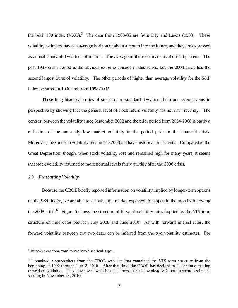
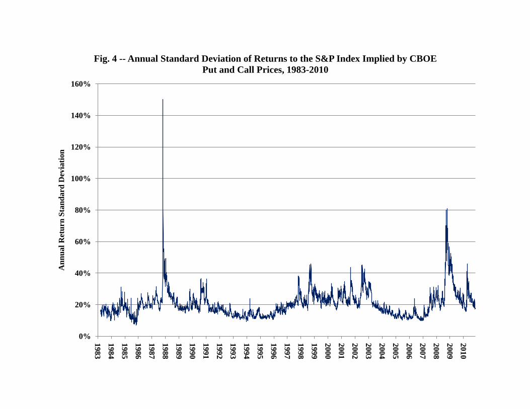
Figure 4 shows one more estimate of the volatility of the Standard & Poor’s index: the

implied volatility of the S&P index measured from put and call prices on “at-the-money” near-term

options of the S&P index that are traded on the CBOE. The data from 1990-2010 are the implied

volatilities of the S&P 500 index (VIX), while the data from 1986-89 are the implied volatilities of

7

the S&P 100 index (VXO).5 The data from 1983-85 are from Day and Lewis (1988). These

volatility estimates have an average horizon of about a month into the future, and they are expressed

as annual standard deviations of returns. The average of these estimates is about 20 percent. The

post-1987 crash period is the obvious extreme episode in this series, but the 2008 crisis has the

second largest burst of volatility. The other periods of higher than average volatility for the S&P

index occurred in 1990 and from 1998-2002.

These long historical series of stock return standard deviations help put recent events in

perspective by showing that the general level of stock return volatility has not risen recently. The

contrast between the volatility since September 2008 and the prior period from 2004-2008 is partly a

reflection of the unusually low market volatility in the period prior to the financial crisis.

Moreover, the spikes in volatility seen in late 2008 did have historical precedents. Compared to the

Great Depression, though, when stock volatility rose and remained high for many years, it seems

that stock volatility returned to more normal levels fairly quickly after the 2008 crisis.

2.3 Forecasting Volatility

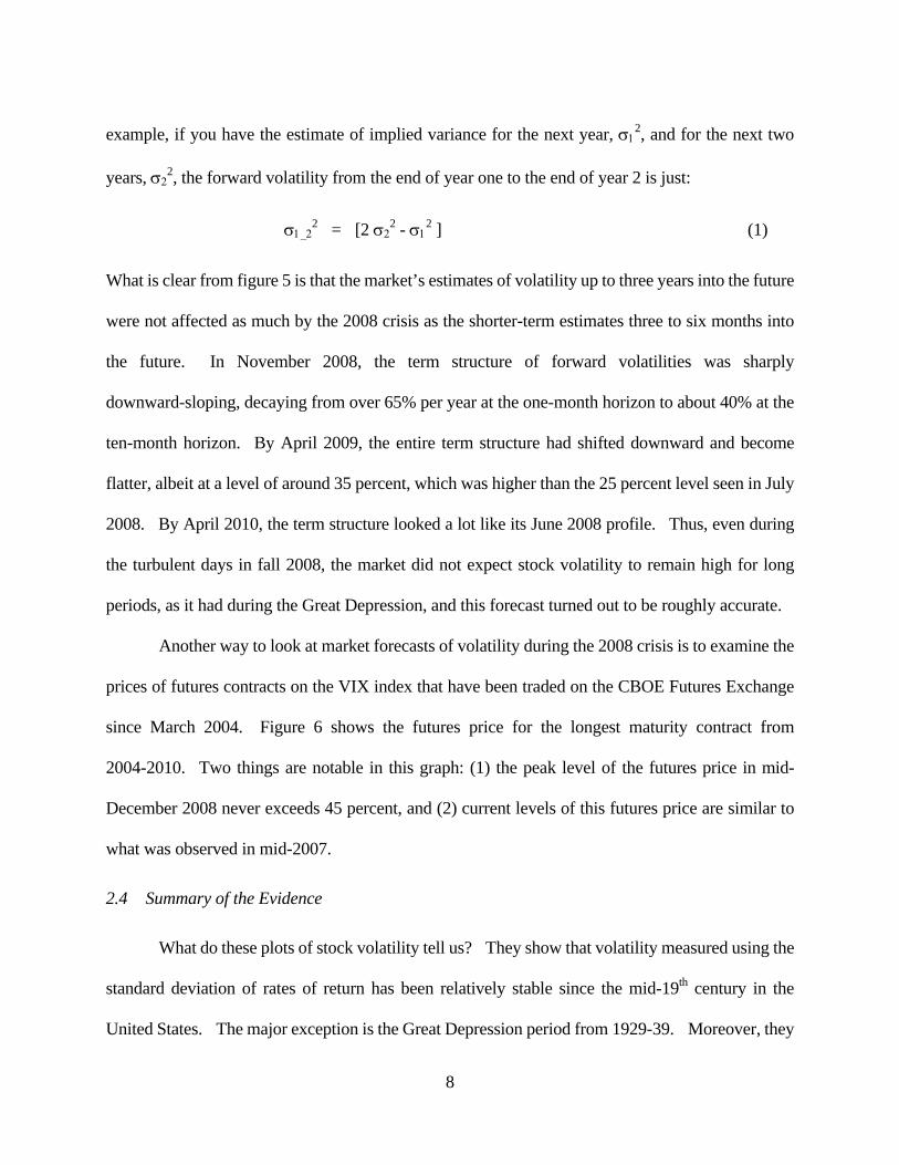
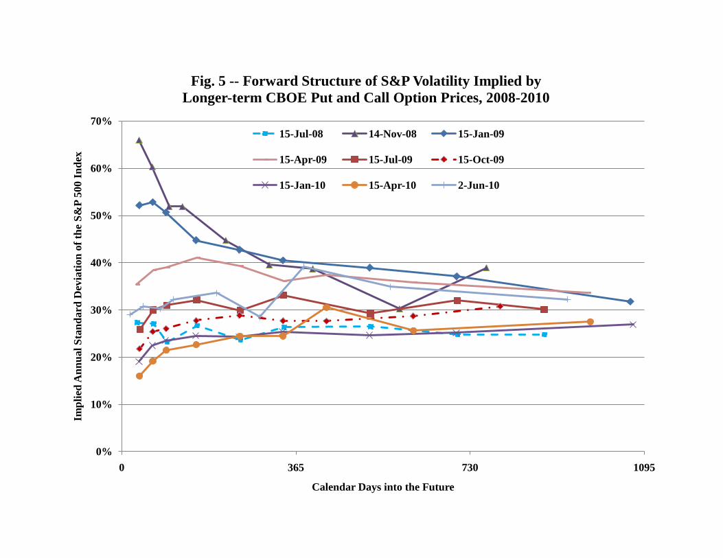
Because the CBOE briefly reported information on volatility implied by longer-term options

on the S&P index, we are able to see what the market expected to happen in the months following

the 2008 crisis.6 Figure 5 shows the structure of forward volatility rates implied by the VIX term

structure on nine dates between July 2008 and June 2010. As with forward interest rates, the

forward volatility between any two dates can be inferred from the two volatility estimates. For

5 http://www.cboe.com/micro/vix/historical.aspx. 6 I obtained a spreadsheet from the CBOE web site that contained the VIX term structure from the beginning of 1992 through June 2, 2010. After that time, the CBOE has decided to discontinue making these data available. They now have a web site that allows users to download VIX term structure estimates starting in November 24, 2010.

8

example, if you have the estimate of implied variance for the next year, 2, and for the next two

years, 2, the forward volatility from the end of year one to the end of year 2 is just:

2 = [2

2 - 2 ] (1)

What is clear from figure 5 is that the market’s estimates of volatility up to three years into the future

were not affected as much by the 2008 crisis as the shorter-term estimates three to six months into

the future. In November 2008, the term structure of forward volatilities was sharply

downward-sloping, decaying from over 65% per year at the one-month horizon to about 40% at the

ten-month horizon. By April 2009, the entire term structure had shifted downward and become

flatter, albeit at a level of around 35 percent, which was higher than the 25 percent level seen in July

2008. By April 2010, the term structure looked a lot like its June 2008 profile. Thus, even during

the turbulent days in fall 2008, the market did not expect stock volatility to remain high for long

periods, as it had during the Great Depression, and this forecast turned out to be roughly accurate.

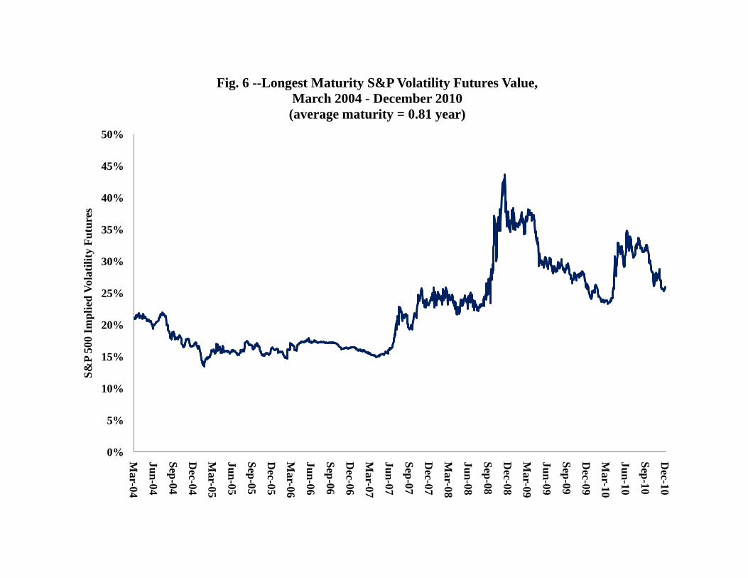
Another way to look at market forecasts of volatility during the 2008 crisis is to examine the

prices of futures contracts on the VIX index that have been traded on the CBOE Futures Exchange

since March 2004. Figure 6 shows the futures price for the longest maturity contract from

2004-2010. Two things are notable in this graph: (1) the peak level of the futures price in mid-

December 2008 never exceeds 45 percent, and (2) current levels of this futures price are similar to

what was observed in mid-2007.

2.4 Summary of the Evidence

What do these plots of stock volatility tell us? They show that volatility measured using the

standard deviation of rates of return has been relatively stable since the mid-19th century in the

United States. The major exception is the Great Depression period from 1929-39. Moreover, they

9

show that the high levels of volatility following recent periods of market stress, such as 1987 and

2008, have been short-lived. These conclusions are not sensitive to whether volatility is measured

from monthly returns, daily returns, or 15 minute returns. Finally, futures returns are more volatile

than stock index returns in periods when there are big price movements. The next section of the

paper studies the behavior of volatility in markets outside the United States, and the following

section analyzes the volatility of different industry sectors to show the extent of the 2008 crisis in

financial markets.

3. Volatility in Other Countries

3.1 Volatility of U.K. Stock Returns

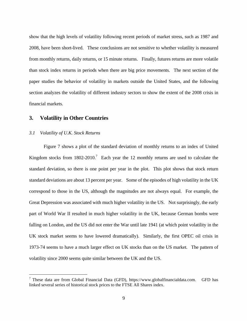
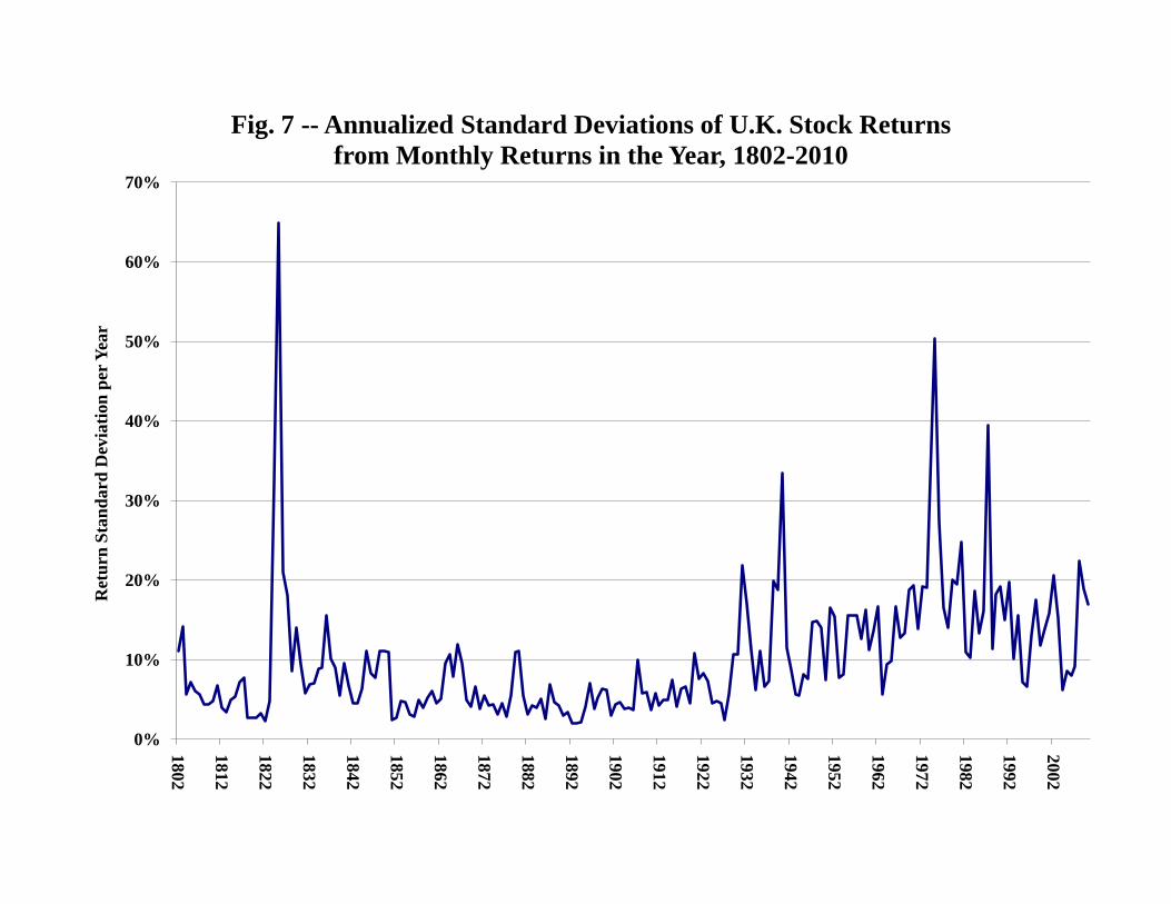
Figure 7 shows a plot of the standard deviation of monthly returns to an index of United

Kingdom stocks from 1802-2010.7 Each year the 12 monthly returns are used to calculate the

standard deviation, so there is one point per year in the plot. This plot shows that stock return

standard deviations are about 13 percent per year. Some of the episodes of high volatility in the UK

correspond to those in the US, although the magnitudes are not always equal. For example, the

Great Depression was associated with much higher volatility in the US. Not surprisingly, the early

part of World War II resulted in much higher volatility in the UK, because German bombs were

falling on London, and the US did not enter the War until late 1941 (at which point volatility in the

UK stock market seems to have lowered dramatically). Similarly, the first OPEC oil crisis in

1973-74 seems to have a much larger effect on UK stocks than on the US market. The pattern of

volatility since 2000 seems quite similar between the UK and the US.

7 These data are from Global Financial Data (GFD), https://www.globalfinancialdata.com. GFD has linked several series of historical stock prices to the FTSE All Shares index.

10

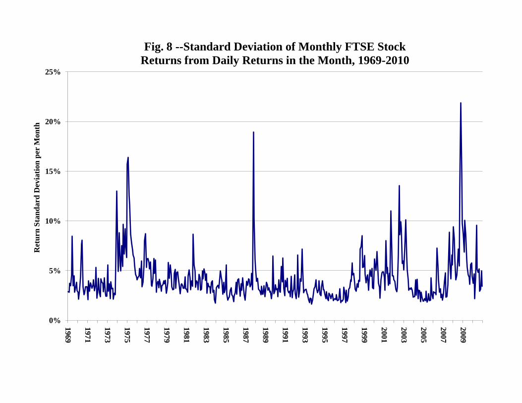
Figure 8 shows a plot of the standard deviation of monthly returns to the Financial Times All

Shares Index (FTSE) from 1969-2010.8 As with figure 2, each month the daily returns are used to

calculate the standard deviation for the month. October 2008 stands out in figure 8, along with

October 1987, as extreme spikes in volatility. Those months were surrounded by high volatility, at

levels comparable with the 1973-75 OPEC period, and the 2002-2003 period. As in the US,

volatility has returned to more normal levels since mid-2009.

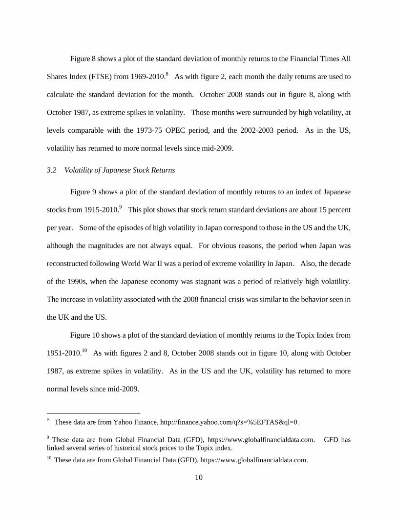
3.2 Volatility of Japanese Stock Returns

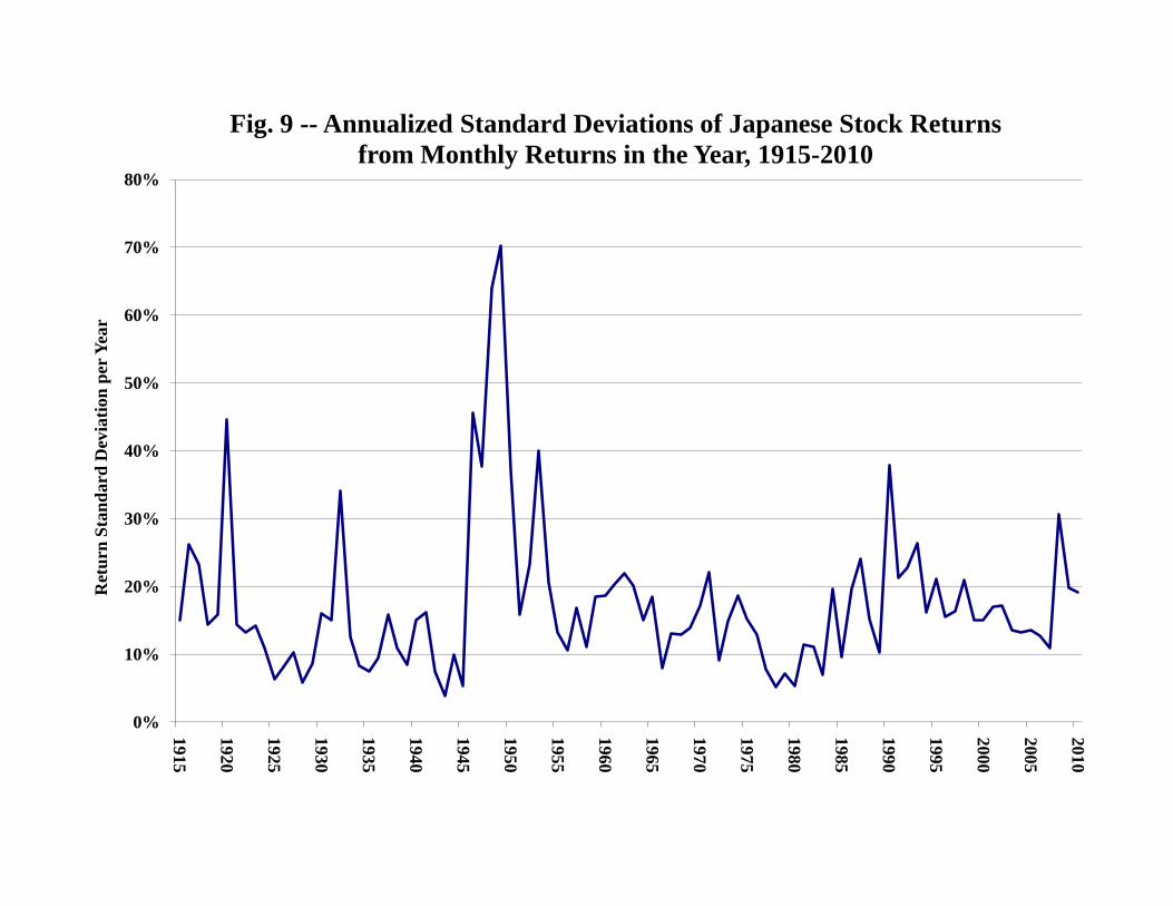
Figure 9 shows a plot of the standard deviation of monthly returns to an index of Japanese

stocks from 1915-2010.9 This plot shows that stock return standard deviations are about 15 percent

per year. Some of the episodes of high volatility in Japan correspond to those in the US and the UK,

although the magnitudes are not always equal. For obvious reasons, the period when Japan was

reconstructed following World War II was a period of extreme volatility in Japan. Also, the decade

of the 1990s, when the Japanese economy was stagnant was a period of relatively high volatility.

The increase in volatility associated with the 2008 financial crisis was similar to the behavior seen in

the UK and the US.

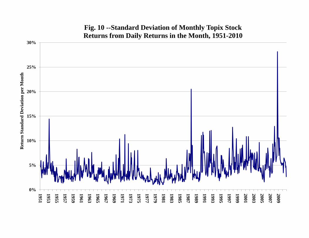
Figure 10 shows a plot of the standard deviation of monthly returns to the Topix Index from

1951-2010.10 As with figures 2 and 8, October 2008 stands out in figure 10, along with October

1987, as extreme spikes in volatility. As in the US and the UK, volatility has returned to more

normal levels since mid-2009.

8 These data are from Yahoo Finance, http://finance.yahoo.com/q?s=%5EFTAS&ql=0. 9 These data are from Global Financial Data (GFD), https://www.globalfinancialdata.com. GFD has linked several series of historical stock prices to the Topix index. 10 These data are from Global Financial Data (GFD), https://www.globalfinancialdata.com.

11

Thus, the financial crisis had similar effects in the major stock markets around the world.

Most importantly, the periods of very high volatility in daily stock returns were short-lived.

4. Volatility in Sectors of the Market

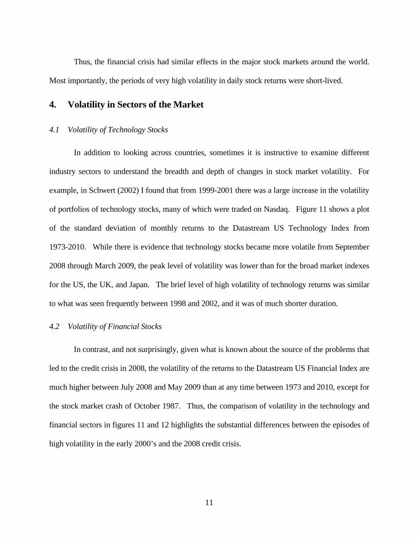
4.1 Volatility of Technology Stocks

In addition to looking across countries, sometimes it is instructive to examine different

industry sectors to understand the breadth and depth of changes in stock market volatility. For

example, in Schwert (2002) I found that from 1999-2001 there was a large increase in the volatility

of portfolios of technology stocks, many of which were traded on Nasdaq. Figure 11 shows a plot

of the standard deviation of monthly returns to the Datastream US Technology Index from

1973-2010. While there is evidence that technology stocks became more volatile from September

2008 through March 2009, the peak level of volatility was lower than for the broad market indexes

for the US, the UK, and Japan. The brief level of high volatility of technology returns was similar

to what was seen frequently between 1998 and 2002, and it was of much shorter duration.

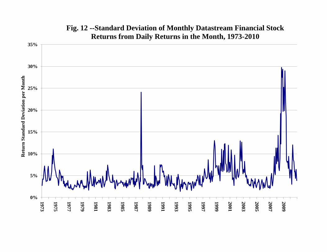
4.2 Volatility of Financial Stocks

In contrast, and not surprisingly, given what is known about the source of the problems that

led to the credit crisis in 2008, the volatility of the returns to the Datastream US Financial Index are

much higher between July 2008 and May 2009 than at any time between 1973 and 2010, except for

the stock market crash of October 1987. Thus, the comparison of volatility in the technology and

financial sectors in figures 11 and 12 highlights the substantial differences between the episodes of

high volatility in the early 2000’s and the 2008 credit crisis.

12

5. Stock Volatility as a Leading Indicator

The survey of the behavior of stock return volatility across different measurement intervals,

different countries, and different industries shows that there was a large burst of volatility in

mid-2008 that lasted for less than a year. While the magnitude and duration of the increase in

volatility differed somewhat, the general pattern was quite consistent. Moreover, the relatively

quick dissipation of the high levels of volatility was accurately anticipated by the financial markets,

even at the time of the highest short-term volatility.

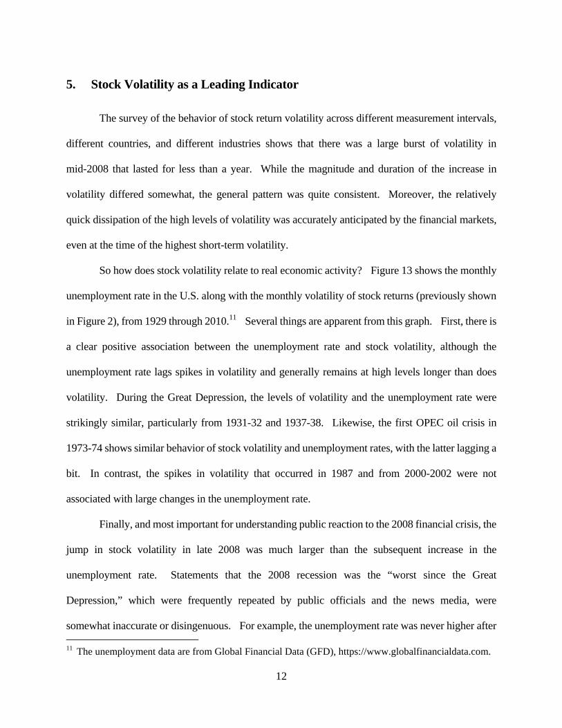
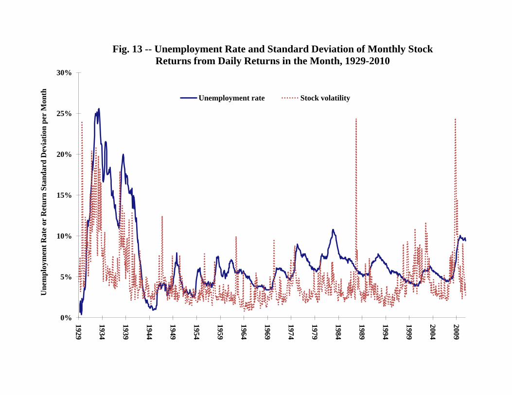
So how does stock volatility relate to real economic activity? Figure 13 shows the monthly

unemployment rate in the U.S. along with the monthly volatility of stock returns (previously shown

in Figure 2), from 1929 through 2010.11 Several things are apparent from this graph. First, there is

a clear positive association between the unemployment rate and stock volatility, although the

unemployment rate lags spikes in volatility and generally remains at high levels longer than does

volatility. During the Great Depression, the levels of volatility and the unemployment rate were

strikingly similar, particularly from 1931-32 and 1937-38. Likewise, the first OPEC oil crisis in

1973-74 shows similar behavior of stock volatility and unemployment rates, with the latter lagging a

bit. In contrast, the spikes in volatility that occurred in 1987 and from 2000-2002 were not

associated with large changes in the unemployment rate.

Finally, and most important for understanding public reaction to the 2008 financial crisis, the

jump in stock volatility in late 2008 was much larger than the subsequent increase in the

unemployment rate. Statements that the 2008 recession was the “worst since the Great

Depression,” which were frequently repeated by public officials and the news media, were

somewhat inaccurate or disingenuous. For example, the unemployment rate was never higher after 11 The unemployment data are from Global Financial Data (GFD), https://www.globalfinancialdata.com.

13

September 2008 than it was between September 1982 and June 1983. While stock volatility was

briefly at levels similar to those seen during the Great Depression in late 2008, the unemployment

rate was never half as high as it was during the periods of high stock volatility during the Great

Depression.

Of course, the reason why stock volatility can color public perceptions of economic

conditions is that is so easily visible in real time. The availability of financial information,

including direct measures of volatility expectations in the form of the VIX index, provides the news

media and politicians with ammunition for stories of imminent economic disaster. Most measures

of real activity, such as the unemployment rate, are only available with a substantial lag because of

normal measurement processes.

6. Summary and Conclusions

The financial crisis in late 2008 was a major disruption to the financial sector. There has

been much discussion about the causes and consequences that led to the failure or near failure of

many large financial institutions, and there have been many proposals to assure that a similar credit

crisis will be less likely to happen in the future.

One of the most visible indicators of the crisis that captured the attention of the general

public was the extremely high level of stock return volatility. This uncertainty prompted much

speculation and discussion about the likely real economic consequences of the credit crisis. This

paper has shown that the spike in stock volatility occurred in many countries. Volatility was

highest among stocks in the financial sector, but it was also high market-wide.

From the contingent claims markets there is direct evidence that market participants did not

expect the high levels of volatility to persist for long periods. It turns out that these expectations

14

were realized, because stock volatility returned to much more normal levels within months. Thus,

the comparisons with the Great Depression that have occurred frequently over the last few years are

exaggerated or misguided.

15

References

Day, Theodore E. and Craig M. Lewis, "The Behavior of the Volatility Implicit in the Prices of Stock Index Options," Journal of Financial Economics, 22 (1988) 103-122.

Schwert, G. William, "Indexes of United States Stock Prices from 1802 to 1987," Journal

of Business, 63 (July 1990) 399-426.

Schwert, G. William, "Stock Volatility in the New Millennium: How Wacky is Nasdaq?" Journal of Monetary Economics, 49 (January 2002) 3-26.

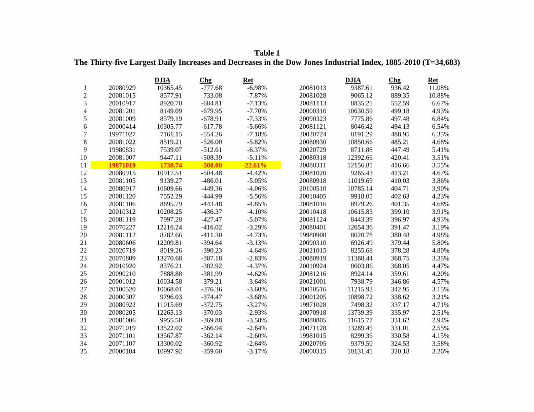
Table 1 The Thirty-five Largest Daily Increases and Decreases in the Dow Jones Industrial Index, 1885-2010 (T=34,683)

DJIA Chg Ret

DJIA Chg Ret

1 20080929 10365.45 -777.68 -6.98%

20081013 9387.61 936.42 11.08% 2 20081015 8577.91 -733.08 -7.87%

20081028 9065.12 889.35 10.88%

3 20010917 8920.70 -684.81 -7.13%

20081113 8835.25 552.59 6.67% 4 20081201 8149.09 -679.95 -7.70%

20000316 10630.59 499.18 4.93%

5 20081009 8579.19 -678.91 -7.33%

20090323 7775.86 497.48 6.84% 6 20000414 10305.77 -617.78 -5.66%

20081121 8046.42 494.13 6.54%

7 19971027 7161.15 -554.26 -7.18%

20020724 8191.29 488.95 6.35% 8 20081022 8519.21 -526.00 -5.82%

20080930 10850.66 485.21 4.68%

9 19980831 7539.07 -512.61 -6.37%

20020729 8711.88 447.49 5.41% 10 20081007 9447.11 -508.39 -5.11%

20080318 12392.66 420.41 3.51%

11 19871019 1738.74 -508.00 -22.61%

20080311 12156.81 416.66 3.55% 12 20080915 10917.51 -504.48 -4.42%

20081020 9265.43 413.21 4.67%

13 20081105 9139.27 -486.01 -5.05%

20080918 11019.69 410.03 3.86% 14 20080917 10609.66 -449.36 -4.06%

20100510 10785.14 404.71 3.90%

15 20081120 7552.29 -444.99 -5.56%

20010405 9918.05 402.63 4.23% 16 20081106 8695.79 -443.48 -4.85%

20081016 8979.26 401.35 4.68%

17 20010312 10208.25 -436.37 -4.10%

20010418 10615.83 399.10 3.91% 18 20081119 7997.28 -427.47 -5.07%

20081124 8443.39 396.97 4.93%

19 20070227 12216.24 -416.02 -3.29%

20080401 12654.36 391.47 3.19% 20 20081112 8282.66 -411.30 -4.73%

19980908 8020.78 380.48 4.98%

21 20080606 12209.81 -394.64 -3.13%

20090310 6926.49 379.44 5.80% 22 20020719 8019.26 -390.23 -4.64%

20021015 8255.68 378.28 4.80%

23 20070809 13270.68 -387.18 -2.83%

20080919 11388.44 368.75 3.35% 24 20010920 8376.21 -382.92 -4.37%

20010924 8603.86 368.05 4.47%

25 20090210 7888.88 -381.99 -4.62%

20081216 8924.14 359.61 4.20% 26 20001012 10034.58 -379.21 -3.64%

20021001 7938.79 346.86 4.57%

27 20100520 10068.01 -376.36 -3.60%

20010516 11215.92 342.95 3.15% 28 20000307 9796.03 -374.47 -3.68%

20001205 10898.72 338.62 3.21%

29 20080922 11015.69 -372.75 -3.27%

19971028 7498.32 337.17 4.71% 30 20080205 12265.13 -370.03 -2.93%

20070918 13739.39 335.97 2.51%

31 20081006 9955.50 -369.88 -3.58%

20080805 11615.77 331.62 2.94% 32 20071019 13522.02 -366.94 -2.64%

20071128 13289.45 331.01 2.55%

33 20071101 13567.87 -362.14 -2.60%

19981015 8299.36 330.58 4.15% 34 20071107 13300.02 -360.92 -2.64%

20020705 9379.50 324.53 3.58%

35 20000104 10997.92 -359.60 -3.17%

20000315 10131.41 320.18 3.26%

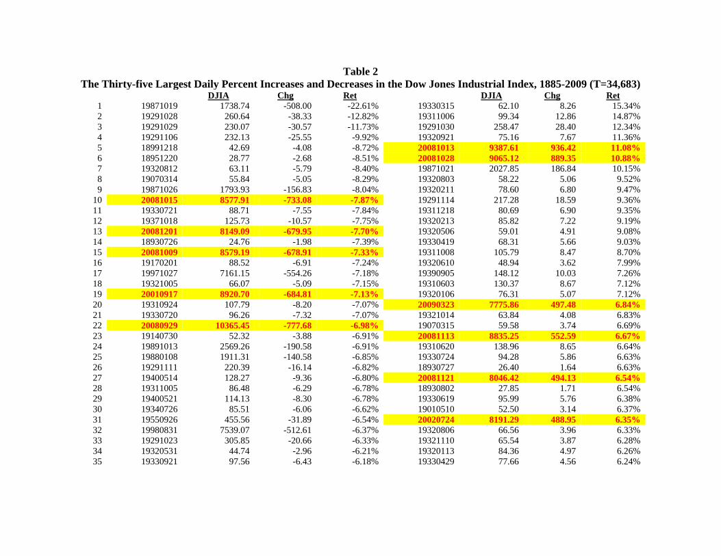
Table 2 The Thirty-five Largest Daily Percent Increases and Decreases in the Dow Jones Industrial Index, 1885-2009 (T=34,683)

DJIA Chg Ret

DJIA Chg Ret

1 19871019 1738.74 -508.00 -22.61% 19330315 62.10 8.26 15.34% 2 19291028 260.64 -38.33 -12.82% 19311006 99.34 12.86 14.87% 3 19291029 230.07 -30.57 -11.73% 19291030 258.47 28.40 12.34% 4 19291106 232.13 -25.55 -9.92% 19320921 75.16 7.67 11.36% 5 18991218 42.69 -4.08 -8.72% 20081013 9387.61 936.42 11.08% 6 18951220 28.77 -2.68 -8.51% 20081028 9065.12 889.35 10.88% 7 19320812 63.11 -5.79 -8.40% 19871021 2027.85 186.84 10.15% 8 19070314 55.84 -5.05 -8.29% 19320803 58.22 5.06 9.52% 9 19871026 1793.93 -156.83 -8.04% 19320211 78.60 6.80 9.47%

10 20081015 8577.91 -733.08 -7.87% 19291114 217.28 18.59 9.36% 11 19330721 88.71 -7.55 -7.84% 19311218 80.69 6.90 9.35% 12 19371018 125.73 -10.57 -7.75% 19320213 85.82 7.22 9.19% 13 20081201 8149.09 -679.95 -7.70% 19320506 59.01 4.91 9.08% 14 18930726 24.76 -1.98 -7.39% 19330419 68.31 5.66 9.03% 15 20081009 8579.19 -678.91 -7.33% 19311008 105.79 8.47 8.70% 16 19170201 88.52 -6.91 -7.24% 19320610 48.94 3.62 7.99% 17 19971027 7161.15 -554.26 -7.18% 19390905 148.12 10.03 7.26% 18 19321005 66.07 -5.09 -7.15% 19310603 130.37 8.67 7.12% 19 20010917 8920.70 -684.81 -7.13% 19320106 76.31 5.07 7.12% 20 19310924 107.79 -8.20 -7.07% 20090323 7775.86 497.48 6.84% 21 19330720 96.26 -7.32 -7.07% 19321014 63.84 4.08 6.83% 22 20080929 10365.45 -777.68 -6.98% 19070315 59.58 3.74 6.69% 23 19140730 52.32 -3.88 -6.91% 20081113 8835.25 552.59 6.67% 24 19891013 2569.26 -190.58 -6.91% 19310620 138.96 8.65 6.64% 25 19880108 1911.31 -140.58 -6.85% 19330724 94.28 5.86 6.63% 26 19291111 220.39 -16.14 -6.82% 18930727 26.40 1.64 6.63% 27 19400514 128.27 -9.36 -6.80% 20081121 8046.42 494.13 6.54% 28 19311005 86.48 -6.29 -6.78% 18930802 27.85 1.71 6.54% 29 19400521 114.13 -8.30 -6.78% 19330619 95.99 5.76 6.38% 30 19340726 85.51 -6.06 -6.62% 19010510 52.50 3.14 6.37% 31 19550926 455.56 -31.89 -6.54% 20020724 8191.29 488.95 6.35% 32 19980831 7539.07 -512.61 -6.37% 19320806 66.56 3.96 6.33% 33 19291023 305.85 -20.66 -6.33% 19321110 65.54 3.87 6.28% 34 19320531 44.74 -2.96 -6.21% 19320113 84.36 4.97 6.26% 35 19330921 97.56 -6.43 -6.18% 19330429 77.66 4.56 6.24%

0%

10%

20%

30%

40%

50%

60%

1802

1812

1822

1832

1842

1852

1862

1872

1882

1892

1902

1912

1922

1932

1942

1952

1962

1972

1982

1992

2002R

etur

n St

anda

rd D

evia

tion

per Y

ear

Fig. 1 -- Annualized Standard Deviations of U.S. Stock Returnsfrom Monthly Returns in the Year, 1802-2010

0%

5%

10%

15%

20%

25%

30%

1885

1890

1895

1900

1905

1910

1915

1920

1925

1930

1935

1940

1945

1950

1955

1960

1965

1970

1975

1980

1985

1990

1995

2000

2005

2010

Ret

urn

Sta

nd

ard

Dev

iati

on

per

Mon

thFig. 2 -- Standard Deviation of Monthly Stock Returns

from Daily Returns in the Month, 1885-2010

0%

5%

10%

15%

20%

25%

1982

1983

1984

1985

1986

1987

1988

1989

1990

1991

1992

1993

1994

1995

1996

1997

1998

1999

2000

2001

2002

2003

2004

2005

2006

2007

2008

2009

2010R

etur

n St

anda

rd D

evia

tion

per

Day

Fig. 3 -- Volatility of the S&P 500 and S&P Futures, Based on Intraday 15-minute Returns, 1982-2010

S&P Futures S&P

0%

20%

40%

60%

80%

100%

120%

140%

160%

1983

1984

1985

1986

1987

1988

1989

1990

1991

1992

1993

1994

1995

1996

1997

1998

1999

2000

2001

2002

2003

2004

2005

2006

2007

2008

2009

2010A

nnua

l Ret

urn

Stan

dard

Dev

iatio

nFig. 4 -- Annual Standard Deviation of Returns to the S&P Index Implied by CBOE

Put and Call Prices, 1983-2010

0%

10%

20%

30%

40%

50%

60%

70%

0 365 730 1095

Impl

ied

Ann

ual S

tand

ard

Dev

iatio

n of

the

S&P

500

Inde

x

Calendar Days into the Future

Fig. 5 -- Forward Structure of S&P Volatility Implied by Longer-term CBOE Put and Call Option Prices, 2008-2010

15-Jul-08 14-Nov-08 15-Jan-09

15-Apr-09 15-Jul-09 15-Oct-09

15-Jan-10 15-Apr-10 2-Jun-10

0%

5%

10%

15%

20%

25%

30%

35%

40%

45%

50%

Mar-04

Jun-04

Sep-04

Dec-04

Mar-05

Jun-05

Sep-05

Dec-05

Mar-06

Jun-06

Sep-06

Dec-06

Mar-07

Jun-07

Sep-07

Dec-07

Mar-08

Jun-08

Sep-08

Dec-08

Mar-09

Jun-09

Sep-09

Dec-09

Mar-10

Jun-10

Sep-10

Dec-10

S&P

500

Impl

ied

Vola

tility

Fut

ures

Fig. 6 --Longest Maturity S&P Volatility Futures Value,March 2004 - December 2010(average maturity = 0.81 year)

0%

10%

20%

30%

40%

50%

60%

70%

1802

1812

1822

1832

1842

1852

1862

1872

1882

1892

1902

1912

1922

1932

1942

1952

1962

1972

1982

1992

2002

Ret

urn

Sta

nd

ard

Dev

iati

on

per

Yea

r

Fig. 7 -- Annualized Standard Deviations of U.K. Stock Returns

from Monthly Returns in the Year, 1802-2010

0%

5%

10%

15%

20%

25%

1969

1971

1973

1975

1977

1979

1981

1983

1985

1987

1989

1991

1993

1995

1997

1999

2001

2003

2005

2007

2009

Ret

urn

Sta

nd

ard

Dev

iati

on

per

Mon

th

Fig. 8 --Standard Deviation of Monthly FTSE Stock

Returns from Daily Returns in the Month, 1969-2010

0%

10%

20%

30%

40%

50%

60%

70%

80%

1915

1920

1925

1930

1935

1940

1945

1950

1955

1960

1965

1970

1975

1980

1985

1990

1995

2000

2005

2010

Ret

urn

Sta

nd

ard

Dev

iati

on

per

Yea

r

Fig. 9 -- Annualized Standard Deviations of Japanese Stock Returns

from Monthly Returns in the Year, 1915-2010

0%

5%

10%

15%

20%

25%

30%

1951

1953

1955

1957

1959

1961

1963

1965

1967

1969

1971

1973

1975

1977

1979

1981

1983

1985

1987

1989

1991

1993

1995

1997

1999

2001

2003

2005

2007

2009

Ret

urn

Sta

nd

ard

Dev

iati

on

per

Mon

th

Fig. 10 --Standard Deviation of Monthly Topix Stock

Returns from Daily Returns in the Month, 1951-2010

0%

5%

10%

15%

20%

25%

30%

35%

1973

1975

1977

1979

1981

1983

1985

1987

1989

1991

1993

1995

1997

1999

2001

2003

2005

2007

2009

Ret

urn

Sta

nd

ard

Dev

iati

on

per

Mon

th

Fig. 11 --Standard Deviation of Monthly Datastream Technology Stock

Returns from Daily Returns in the Month, 1973-2010

0%

5%

10%

15%

20%

25%

30%

35%

1973

1975

1977

1979

1981

1983

1985

1987

1989

1991

1993

1995

1997

1999

2001

2003

2005

2007

2009

Ret

urn

Sta

nd

ard

Dev

iati

on

per

Mon

th

Fig. 12 --Standard Deviation of Monthly Datastream Financial Stock

Returns from Daily Returns in the Month, 1973-2010

0%

5%

10%

15%

20%

25%

30%

1929

1934

1939

1944

1949

1954

1959

1964

1969

1974

1979

1984

1989

1994

1999

2004

2009U

nem

ploy

men

t Rat

e or

Ret

urn

Stan

dard

Dev

iatio

n pe

r M

onth

Fig. 13 -- Unemployment Rate and Standard Deviation of Monthly Stock Returns from Daily Returns in the Month, 1929-2010

Unemployment rate Stock volatility