1

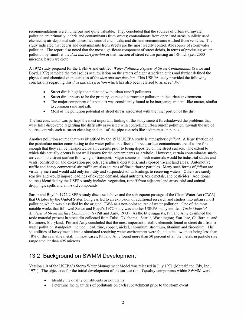
Stormwater Quality Modeling Improvements Needed For SWMM

Roger C. Sutherland, PE, and Seth L. Jelen, PE Pacific Water Resources, Inc. 4905 SW Griffith Drive, Suite 200 Beaverton, Oregon 97005 Ph: (503) 671-9709 Fax: (503) 671-0711 E-mail: info@pacificwr.com The U.S. Environmental Protection Agency’s (USEPA) Stormwater Management Model, or SWMM, is a large, relatively complex software package capable of simulating the transformation of precipitation to urban runoff and the transport of the runoff from the ground surface through pipe/channel networks and storage/treatment facilities and finally to receiving waters. The model can be used to simulate a single event or a long continuous period. The original model was developed by Metcalf and Eddy, Inc. in association with the University of Florida and Water Resources Engineers, Inc. in 1971. Over the last three decades there have been many significant improvements and enhancements to the model’s capabilities. However, the model’s algorithms used to simulate the accumulation and transport of stormwater pollutants have rarely been addressed or significantly improved. With the recent development of the USEPA’s NPDES stormwater program and the ongoing development of the TMDL program and the continuing interest and concern associated with stormwater pollution throughout the developed world, the need to significantly improve the stormwater quality modeling capabilities of SWMM is greater now than ever before. This paper will review the model’s existing stormwater quality algorithms, discuss the problems associated with these algorithms and offer a specific outline of needed improvements. The modeling insights and improvements are based on knowledge gained through many years of study and research that has led to the development of the Simplified Particulate Transport Model (SIMPTM) (Sutherland and Jelen, 1998) which has been recently applied to projects in Michigan, Oregon and Washington. The suggested improvements are, in general, algorithms that are already incorporated into SIMPTM. It is the understanding of the authors that an effort is currently underway by USEPA, Camp Dresser and McKee (CDM) and Dr. Wayne Huber to significantly improve the existing SWMM code and create SWMM Version 5.0. In an effort to fully cooperate, the authors have provided Mr. Robert Dickerson of CDM with existing SIMPTM computer code and documentation. The hope would be that all of the water quality related improvements recommended in this paper will be included in the new SWMM 5.0. If that occurred, SWMM would be able to more accurately simulate important urban stormwater pollution processes including the pollutant removal effectiveness of both street and catchbasin cleaning practices. 13.1 Background on Stormwater Pollution Sources The first serious attempt to identify the specific sources of urban runoff pollution that had been observed by so many researchers since 1948 throughout the world occurred in the American Public Works Association’s 1969 Chicago study (APWA, 1969). The objectives of the study were to investigate the sources of urban stormwater pollution and their magnitudes. The report was principally concerned with evaluating those factors influenced by public works practices that could be affected by changes in governmental operations. The researcher’s conclusions and

2

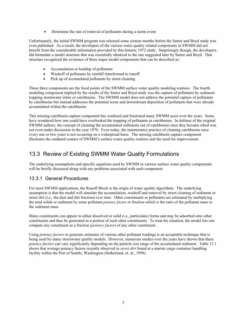
recommendations were numerous and quite valuable. They concluded that the sources of urban stormwater pollution are primarily: debris and contaminants from streets; contaminants from open land areas; publicly used chemicals; air-deposited substances; ice control chemicals; and dirt and contaminants washed from vehicles. The study indicated that debris and contaminants from streets are the most readily controllable source of stormwater pollution. The report also noted that the most significant component of street debris, in terms of producing water pollution by runoff is the dust and dirt fraction or that fraction of street refuse passing an 1/8-inch (i.e., 2000 microns) hardware cloth. A 1972 study prepared for the USEPA and entitled, Water Pollution Aspects of Street Contaminants (Sartor and Boyd, 1972) sampled the total solids accumulation on the streets of eight American cities and further defined the physical and chemical characteristics of the dust and dirt fraction. This USEPA study provided the following conclusions regarding this dust and dirt fraction which has also been referred to as street dirt.

• Street dirt is highly contaminated with urban runoff pollutants. • Street dirt appears to be the primary source of stormwater pollution in the urban environment. • The major component of street dirt was consistently found to be inorganic; mineral-like matter, similar

to common sand and silt. • Most of the pollution potential of street dirt is associated with the finer portion of the dirt.

The last conclusion was perhaps the most important finding of the study since it foreshadowed the problems that were later discovered regarding the difficulty associated with controlling urban runoff pollution through the use of source controls such as street cleaning and end-of-the-pipe controls like sedimentation ponds. Another pollution source that was identified by the 1972 USEPA study is atmospheric fallout. A large fraction of the particulate matter contributing to the water pollution effects of street surface contaminants are of a size fine enough that they can be transported by air currents prior to being deposited on the street surface. The extent to which this actually occurs is not well known for the contaminants as a whole. However, certain contaminants surely arrived on the street surface following air transport. Major sources of such materials would be industrial stacks and vents, construction and excavation projects, agricultural operations, and exposed vacant land areas. Automotive traffic and heavy commercial air traffic are also sources of fine airborne particles. Many such forms of fallout are virtually inert and would add only turbidity and suspended solids loadings to receiving waters. Others are surely reactive and would impose loadings of oxygen demand, algal nutrients, toxic metals, and pesticides. Additional sources identified by the USEPA study include: vegetation, runoff from adjacent land areas, bird and animal droppings, spills and anti-skid compounds. Sartor and Boyd’s 1972 USEPA study discussed above and the subsequent passage of the Clean Water Act (CWA) that October by the United States Congress led to an explosion of additional research and studies into urban runoff pollution which was classified by the original CWA as a non-point source of water pollution. One of the most notable works that followed Sartor and Boyd’s 1972 study was another USEPA study entitled, Toxic Material Analysis of Street Surface Contaminants (Pitt and Amy, 1973). As the title suggests, Pitt and Amy examined the toxic material present in street dirt collected from Tulsa, Oklahoma; Seattle, Washington; San Jose, California; and Baltimore, Maryland. Pitt and Amy concluded that the most important metallic elements found in street dirt, from a water pollution standpoint, include: lead, zinc, copper, nickel, chromium, strontium, titanium and zirconium. The solubilities of heavy metals into a simulated receiving water environment were found to be low, most being less than 10% of the available metal. In most cases, Pitt and Amy found more than 50 percent of all the metals in particle size range smaller than 495 microns. 13.2 Background on SWMM Development Version 1.0 of the USEPA’s Storm Water Management Model was released in July 1971 (Metcalf and Edy, Inc., 1971). The objectives for the initial development of the surface runoff quality components within SWMM were:

• Identify the quality constituents or pollutants • Determine the quantities of pollutants on each subcatchment prior to the storm event

3

• Determine the rate of removal of pollutants during a storm event Unfortunately, the initial SWMM program was released some sixteen months before the Sartor and Boyd study was even published. As a result, the developers of the various water quality related components in SWMM did not benefit from the considerable information provided by this historic 1972 study. Surprisingly though, the developers did formulate a model structure that was essentially identical to the one suggested later by Sartor and Boyd. That structure recognized the existence of three major model components that can be described as:

• Accumulation or buildup of pollutants • Washoff of pollutants by rainfall transformed to runoff • Pick up of accumulated pollutants by street cleaning

These three components are the focal points of the SWMM surface water quality modeling routines. The fourth modeling component implied by the results of the Sartor and Boyd study was the capture of pollutants by sediment trapping stormwater inlets or catchbasins. The SWMM model does not address the potential capture of pollutants by catchbasins but instead addresses the potential scour and downstream deposition of pollutants that were already accumulated within the catchbasins. This missing catchbasin capture component has confused and frustrated many SWMM users over the years. Some have wondered how one could have overlooked the trapping of pollutants in catchbasins. In defense of the original SWMM authors, the concept of cleaning the accumulated sediments out of catchbasins once they became silted was not even under discussion in the year 1970. Even today, the maintenance practice of cleaning catchbasins once every one or two years is not occurring on a widespread basis. The missing catchbasin capture component illustrates the outdated contact of SWMM’s surface water quality routines and the need for improvement. 13.3 Review of Existing SWMM Water Quality Formulations The underlying assumptions and specific equations used by SWMM in various surface water quality components will be briefly discussed along with any problems associated with each component. 13.3.1 General Procedures For most SWMM applications, the Runoff Block is the origin of water quality algorithms. The underlying assumption is that the model will simulate the accumulation, washoff and removal by street cleaning of sediment or street dirt (i.e., the dust and dirt fraction) over time. Other constituents or pollutants are estimated by multiplying the total solids or sediment by some pollutant potency factor or fraction which is the ratio of the pollutant mass to the sediment mass Many constituents can appear in either dissolved or solid (i.e., particulate) forms and may be adsorbed onto other constituents and thus be generated as a portion of such other constituents. To treat his situation, the model lets one compute any constituent as a fraction (potency factor) of any other constituent. Using potency factors to generate estimates of various other pollutant loadings is an acceptable technique that is being used by many stormwater quality models. However, numerous studies over the years have shown that these potency factors can vary significantly depending on the particle size range of the accumulated sediment. Table 13.1 shows that average potency factors recently observed in street dirt found at a marine cargo container handling facility within the Port of Seattle, Washington (Sutherland, et. al., 1998).

4

Table13.1 Potency Factors from Sutherland, et. al., 1998.

Parameter

Average Potency Factor by Particle Size Group (mg/kg)

Fine (# tests) Medium (# tests) Coarse (# tests)

Total Copper 248 (12) 161 (12) 263 (12) Total Lead 442 (12) 220 (12) 94 (12) Total Zinc 2167 (12) 1892 (12) 858 (12) TPH 9492 (12) 6832 (12) 3935 (13) COD 165000 (6) 65000 (6) 30100 (6) Ortho Phosphorus

500 (6) 337 (6) 222 (6)

TKN 989 (6) 521 (6) 276 (6) TPH = Total petroleum hydrocarbon Fine = less than 63 microns COD = Chemical oxygen demand Medium = 63 to 250 microns TKN = Total kjeldahl nitrogen Coarse = 251 to 2000 microns 13.3.2 Accumulation Component The accumulation equations used in SWMM refer to the dust and dirt fraction identified in the APWA 1969 study which was sediment or street dirt accumulated on the streets of Chicago. However, the user can choose to conceptualize the accumulation as occurring throughout the entire subcatchment area by selecting the parameter units as pounds per acre or pounds per 100 feet of curb which would represent a street loading. The magnitude of the accumulation is a function of the length of the antecedent dry weather preceding the storm. This antecedent time has been referred to as DRYDAYS. Four different buildup equations are currently available in SWMM. Figure 13.1 presents these equations and shows a comparison of the one linear and three non-linear buildup equations (Huber, et. al., 1981). The exponential accumulation equation is probably the most popular since many street dirt accumulation datasets have been analyzed with this equation to derive the best fit equation parameters (Sutherland and Jelen, 1998).

Figure 13.1 Buildup equations available in SWMM (from Huber et.al., 1981).

There are several problems with the accumulation equations within SWMM. First, the accumulation equations do not account for any wet weather accumulation or washon that occurs in urban areas (Sutherland and Jelen, 1996). Wet weather accumulation or washon is the increase in loading that is often observed to result when washoff from

5

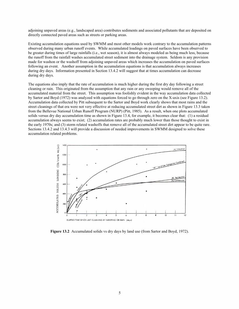
adjoining unpaved areas (e.g., landscaped area) contributes sediments and associated pollutants that are deposited on directly connected paved areas such as streets or parking areas. Existing accumulation equations used by SWMM and most other models work contrary to the accumulation patterns observed during many urban runoff events. While accumulated loadings on paved surfaces have been observed to be greater during times of large rainfalls (i.e., wet season), it is almost always modeled as being much less, because the runoff from the rainfall washes accumulated street sediment into the drainage system. Seldom is any provision made for washon or the washoff from adjoining unpaved areas which increases the accumulation on paved surfaces following an event. Another assumption in the accumulation equations is that accumulation always increases during dry days. Information presented in Section 13.4.2 will suggest that at times accumulation can decrease during dry days. The equations also imply that the rate of accumulation is much higher during the first dry day following a street cleaning or rain. This originated from the assumption that any rain or any sweeping would remove all of the accumulated material from the street. This assumption was foolishly evident in the way accumulation data collected by Sartor and Boyd (1972) was analyzed with equations forced to go through zero on the X-axis (see Figure 13.2). Accumulation data collected by Pitt subsequent to the Sartor and Boyd work clearly shows that most rains and the street cleanings of that era were not very effective at reducing accumulated street dirt as shown in Figure 13.3 taken from the Bellevue National Urban Runoff Program (NURP) (Pitt, 1985). As a result, when one plots accumulated solids versus dry day accumulation time as shown in Figure 13.4, for example, it becomes clear that: (1) a residual accumulation always seems to exist; (2) accumulation rates are probably much lower than those thought to exist in the early 1970s; and (3) storm related washoffs that remove all of the accumulated street dirt appear to be quite rare. Sections 13.4.2 and 13.4.3 will provide a discussion of needed improvements in SWMM designed to solve these accumulation related problems.

Figure 13.2 Accumulated solids vs dry days by land use (from Sartor and Boyd, 1972).

6

Figure 13.3 Observed street dirt loadings from Bellevue NURP (Pitt, 1985).

Figure 13.4 Accumulated solids vs dry days from Bellevue NURP (Pitt, 1985).

7

13.3.3 Washoff Component Version 4 of SWMM released in August 1988 supports two different methods for computing the washoff of pollutants accumulated on the land surface (Huber and Dickerson, 1988). The first method is referred to as the exponential washoff equation which was formulated by the original authors of the model in the early 1970s. The second method, added much later, is referred to as the rating curve approach in which loads (i.e., mass/time) are proportional to flow raised to some power. If the rating curve approach to washoff is used, the accumulation or buildup equations are not needed. The SWMM user’s manual states that the (rating curve) approach may also be justified physically and is often easier to calibrate using available data. Unfortunately, this simple approach does not provide for any linkage to the upland land surfaces where the loading originated from nor does it allow the user to evaluate the effectiveness of any controls which renders it fairly useless. Thus, the focus of the washoff discussion will be on the use of the exponential washoff equation. Very little stormwater quality data existed when the original SWMM model was formulated. The most extensive rainfall to runoff study at the time that included water quality monitoring was conducted on a 17-acre residential and light commercial, urban watershed located in the Mt. Washington section of Cincinnati, Ohio (Weibel, et. al., 1964). For a two-year period starting in July 1962, the rainfall depth, runoff quantity, and runoff quality were continuously monitored. The Cincinnati data had a tremendous influence on the early development of the exponential washoff equation. Mr. Alan Burdoin, a consultant to Mecalf and Eddy during the original SWMM development, theorized that at the start of the rain, the amount of a particular pollutant on surfaces that produce runoff will be PSHED0 in pounds. He also assumed that the mass of pollutant washed off the surface in any time interval (dt) is proportional to the mass remaining on the surface, PSHED. The first order differential equation is: dPSHED/dt = -K . PSHED (13.1) which integrates to: PSHED(t) = PSHED0 e-kt (13.2) where PSHED(t) = quantity of pollutant mass remaining, on the surface at time, t, (h) PSHED0 = initial amount of pollutant mass at start of the rain, and K = coefficient In order to determine K, the SWMM authors assumed that K would vary in direct proportion to the rate of runoff, r: K = RCOEF . r (13.3) where RCOEF = washoff coefficient, depth-1, and r = runoff rate over the subcatchment, depth/time Working with storms from the Cincinnati study, Burdoin assumed that one-half inch of total runoff in one hour would wash off 90 percent of the initial surface load which led to the now famous value of RCOEF of 4.6 in-1. Working with suspended solids data, it was later determined that an availability factor was needed to limit the amount of accumulated pollutant that was available to be washed off. The following equation was created: AV = .057 + 1.4r1.1 (13.4) where AV = availability factor used to determine the fraction of accumulated pollutant available for washoff r = runoff rate over subcatchment, (in/h)

8

The current SWMM model has generalized equation 4 to be: AV = a + brc (13.5) where a,b,c = coefficients The primary difficulty with the use of the exponential washoff equation (i.e., equation 2) is that it will always produce decreasing pollutant concentrations as a function of time regardless of the time distribution of runoff. In other words, it always predicts a first flush phenomena. The first flush is the observation that during a storm event the runoff water that reaches the outflow point first is of the worst quality and the quality of the water draining from the watershed improves as the storm progresses. Clearly this behavior will not be observed if the most intense rainfall occurs in the middle or near the end of the storm. Recognizing this limitation, Version 4 of SWMM attempted to correct this problem by making washoff at each time step, POFF, proportional to runoff rate, r, raised to the power WASHPO as follows: -POFF(t) = dPSHED/dt = -RCOEFX . rWASHPO . PSHED (13.6) where POFF = pollutant mass washed off at time, t PSHED = quantity of pollutant mass available for washoff at time, t RCOEFX, WASHPO = washoff coefficients Two parameters are now needed to simulate pollutant washoff with SWMM. According to the Version 4 manual, availability factors of the form of equation 5 are no longer used since it is believed there is now sufficient flexibility for calibration. Of course, the original SWMM methodology can be recovered by using WASHPO = 1.0. There are several significant problems with the exponential washoff equation within SWMM. The first problem is that the washoff coefficient, RCOEF, can vary dramatically from one storm to the next and there is no apparent way to accurately predict this variation. Working with stormwater data from a 14.7 acre urbanized basin in South Florida, Alley showed that the washoff coefficients for eleven storms collected from May 1977 through June 1978 varied significantly from storm to storm as shown in Table 13.2 (Alley, 1980).

Table 13.2 Optimized Washoff Coefficients (from Alley, 1980).

Optimized RCOEF (inches –1) Storm

Number

Date

Runoff Volume

(in)

Avg. Runoff

Rate (in/hr)

TSS

Total Pb

Total N

1 May 4, 1977 2.6 0.44 0.25 0.34 0.11 2 May 11, 1977 .73 .81 2.8 2.2 1.7 3 June 1, 1977 1.2 .29 1.4 1.6 .78 4 Aug. 8, 1977 .36 .27 2.5 .12 1.9 5 Aug. 8, 1977 .48 .11 -.15 -.15 .49 6 Dec. 12, 1977 .56 .22 5.8 6.2 3.2 7 Mar. 3, 1978 .41 .85 5.7 3.2 3.5 8 Apr. 23, 1978 .48 .22 9.2 5.3 6.1 9 May 18, 1978 .28 .073 11 2.0 2.2

10 May 26, 1978 .47 .22 7.2 5.0 3.0 11 June 12, 1978 .82 .71 .91 .80 .90

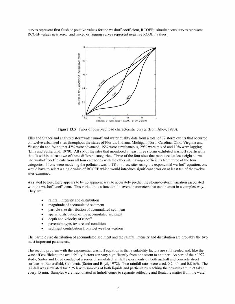
Average Values 4.2 2.4 2.2 Stormwater modelers of the time were focusing on load characteristic curves which were curves that show the plot of cumulative dimensionless constituent pollutant mass washed off by a storm against cumulative dimensionless runoff volume for the same storm. Based on the analysis of storm data, the varying load characteristic curves could be classified as advanced, simultaneous, mixed or lagging as shown in Figure 13.5. Advanced load characteristic

9

curves represent first flush or positive values for the washoff coefficient, RCOEF; simultaneous curves represent RCOEF values near zero; and mixed or lagging curves represent negative RCOEF values.

Figure 13.5 Types of observed load characteristic curves (from Alley, 1980).

Ellis and Sutherland analyzed stormwater runoff and water quality data from a total of 72 storm events that occurred on twelve urbanized sites throughout the states of Florida, Indiana, Michigan, North Carolina, Ohio, Virginia and Wisconsin and found that 42% were advanced, 19% were simultaneous, 29% were mixed and 10% were lagging (Ellis and Sutherland, 1979). All six of the sites that monitored at least three storms exhibited washoff coefficients that fit within at least two of these different categories. Three of the four sites that monitored at least eight storms had washoff coefficients from all four categories with the other site having coefficients from three of the four categories. If one were modeling the pollutant washoff from these sites using the exponential washoff equation, one would have to select a single value of RCOEF which would introduce significant error on at least ten of the twelve sites examined. As stated before, there appears to be no apparent way to accurately predict the storm-to-storm variation associated with the washoff coefficient. This variation is a function of several parameters that can interact in a complex way. They are:

• rainfall intensity and distribution • magnitude of accumulated sediment • particle size distribution of accumulated sediment • spatial distribution of the accumulated sediment • depth and velocity of runoff • pavement type, texture and condition • sediment contribution from wet weather washon

The particle size distribution of accumulated sediment and the rainfall intensity and distribution are probably the two most important parameters. The second problem with the exponential washoff equation is that availability factors are still needed and, like the washoff coefficient, the availability factors can vary significantly from one storm to another. As part of their 1972 study, Sartor and Boyd conducted a series of simulated rainfall experiments on both asphalt and concrete street surfaces in Bakersfield, California (Sartor and Boyd, 1972). Two rainfall rates were used, 0.2 in/h and 0.8 in/h. The rainfall was simulated for 2.25 h with samples of both liquids and particulates reaching the downstream inlet taken every 15 min. Samples were fractionated in Imhoff cones to separate settleable and floatable matter from the water

10

which contained dissolved, colloidal and suspended matter. Each of these fractions was analyzed; the settleable solids were also separated into six particle size ranges by dry sieving. Some results from these tests are presented in Figures 13.6 and 13.7.

Figure 13.6 Solids washoff variation by particle size group (from Sartor and Boyd, 1972).

Figure 13.7 Solids washoff variation by pavement type and rainfall intensity (from Sartor and Boyd, 1972).

The results of these tests were viewed by many early SWMM users as positive proof that the exponential equation was the one to use for washoff simulation since Sartor and Boyd noted that it was the equation that best fit all of their experimental washoff data. Unfortunately, what was missed by the SWMM supporters was the fact that the

11

Sartor and Boyd experiments clearly demonstrated that particulate washoff was a function of particle size and street surface type which are two variables that are not included in the SWMM accumulation or washoff routines. It is interesting to note that one of the most important aspects of these Bakersfield experiments was not reported and essentially overlooked at the time. These tests were conducted on streets that had moderate-to-heavy accumulations of sediments but the magnitude and particle size distribution of the initial conditions were not known. Although the report stated that at the end of the simulation period the streets were flushed thoroughly with a firehouse to wash off any remaining loose or soluble matter and samples of this remaining material were also collected, nothing was reported on how much of the initial load was actually washed off by the simulated rainfall. The assumption made by almost everyone at the time was that essentially all of the initially accumulated sediment was washed off by the simulated runoff event. Personal communications many years later with Dr. Robert Pitt, who worked on the Sartor and Boyd project, revealed the fact that the material washed off appeared to be always just a fraction of what was initially accumulated and in many of the tests the fraction was much smaller than many would assume. In fact, the uncertainty surrounding the initial accumulations of the Bakersfield test and the overall importance of the availability issue in understanding the washoff phenomena motivated Dr. Pitt to repeat a series of similar tests in Toronto, Canada, in 1986 (Pitt and McLean, 1986). Pitt states in his 1987 doctoral dissertation that the Toronto tests were different from the Bakersfield tests in the following ways (Pitt, 1987):

• They were organized in overlapping factorial experimental designs to identify the most important main factors and interactions.

• Particle sizes were measured down to about one micron (in addition to particulate residue and filterable residue measurements).

• The precipitation intensities were lower in order to better represent actual rain conditions of the upper Midwest.

• Observations were made with more resolution at the beginning of the tests. • Washoff flow rates were frequently measured. • Emphasis was placed on total street loading, not just total available loading.

The Toronto washoff tests investigated the washoff of different sized particulates from impervious areas as a function of street texture, street dirt loading and rainfall characteristics. A series of eight controlled washoff tests were conducted on areas that were approximately 3 m by 7 m each. The street side edges of the test areas were lined with plywood, about 30 mm in height and imbedded in thick caulking, needed to direct the runoff towards the curbs with minimal leakage. All runoff was pumped continuously from downstream sumps (sandbags) to graduated containers. The washoff samples were obtained from the pumped water going to the containers every five to ten minutes at the beginning of the tests, and every thirty minutes near the tests’ conclusions. Final complete rinses of the test areas were also conducted (and sampled) at the tests’ conclusions to determine total loadings of the monitored constituents. The samples were analyzed for total residue, filtrate residue, and particulate residue. Runoff samples were also filtered through 0.4 micron filters and the material retained was microscopically analyzed to determine particulate residue size distributions from about 1 to 500 microns. The runoff flow quantities were also carefully monitored to determine the magnitude of initial and total rainwater losses on impervious surfaces. The two extreme levels of the cleanliness factor were for dirty streets (the first sampling run at a site, with obviously dirty streets) and clean streets (the same site, two days after completely flushing the street surface). The eight tests represented all possible combinations of these three factors (except for light rains on dirty, smooth streets, which were actually cleaner than anticipated). The following list summarizes the experimental conditions used, along with the test codings:

• Rain intensity: L: light rain intensity, 2.9 to 3.2 mm/h H: high rain intensity, 11.0 to 12.2 mm/h

• Street cleanliness particulate residue loadings (half street widths were 3.2 to 3.7 m):

12

C: clean streets, 1.7 to 2.6 g/m2 D: dirty streets, 10.5 to 12.6 g/m2

• Pavement texture: R: rough streets, 1.1 mm detention storage S: smooth streets, 0.3 to 0.4 mm detention storage

As an example, the LCR test had a rain intensity of 2.9 mm/h (Light), a half street width of 3.5 m, a total particulate residue loading value of 2.25 g/m2 (Clean), and a street texture expressed as 1.1 mm detention storage (Rough). Plots of cumulative washoff (similar to Figure 13.6) for the HCR (High, Clean and Rough) test are shown on Figure 13.8 as an example since page limitations prevent the reproduction of the other seven test plots. These plots show the asymptotic washoff values observed in the tests, along with the measured total street dirt loading. The maximum asymptotic values are the available street dirt loadings. The measured total loading noted near the top of each plot is significantly larger than these available loadings. For example, the asymptotic total residue value for the HCR test was about 0.8 g/m2 (e.g., available load), or about one quarter the total load of 3.2 g/m2. The differences between available and total loadings for all the tests is shown in Table 13.3 along with the washoff fraction or the availability factor that existed for the conditions of each test.

Figure 13.8 Accumulative washoff plots for HCR test (from Pitt, 1987).

13

Table 13.3 Computed Availability Factors from Toronto Washoff Simulations

Test

Name

Rainfall Intensity

Pavement Texture

Initial Loading

g/m2

Total Estimated Residue Washoff

g/m2

Availability

Factor*

HCR High Rough 3.25 0.84 0.26 LCR Light Rough 2.99 0.58 0.19 HDR High Rough 12.82 1.14 0.09 LDR Light Rough 11.22 0.74 0.07 HCS High Smooth 2.62 1.21 0.46 LCS Light Smooth 2.32 0.35 0.15 HDS High Smooth 13.82 2.74 0.20

L(D)CS** Light Smooth 2.42 0.57 0.24 * Ratio of total washoff to initial accumulation. ** Initial accumulation was much lower than expected, similar to LCS.

Note that the computed availability factors for the total residue washoff ranged from 0.46 to 0.07 with a mean of 0.21. The availability factors for the particulate residue washoff reported by Pitt were even lower with the range from 0.26 to 0.028 with a mean of 0.10. While calibrating the continuous SIMPTM model to washoff data from seven storms observed over 19 months at six sites in Portland, Oregon, Sutherland and Jelen concluded that the overall availability factor for each site ranged from 0.15 to 0.20 (Sutherland and Jelen, 1996). As stated earlier, availability factors are needed and as the Toronto washoff tests show, they can vary significantly from one storm to another. Everything else held constant; availability factors will increase with increasing rainfall intensity, runoff volume and decrease with increasing initial loading, particle sizes and pavement roughness. Section 13.4.4 will provide a discussion of needed improvements in SWMM designed to solve these various washoff related problems. 13.3.4 Street Cleaning Component Within the Runoff Block, street cleaning (usually assumed to be sweeping) is performed (if desired) prior to the beginning of the first storm event and between storm events (for continuous simulation). Unless initial constituent loads are input or unless a rating curve is used, a mini-simulation is performed for each constituent during the dry days prior to a storm in which accumulation and street cleaning are modeled. Starting with zero initial load, accumulation occurs according to the method chosen. Street cleaning occurs at the specified intervals of CLFREQ days as shown in Figure 13.9. Note that during continuous simulation, cleaning occurs between storms based on intervals calculated using dry time steps only. A dry time step does not have runoff greater than 0.0005 in/h (0.13 mm/h), nor is snow present on the impervious area of the catchment. If runoff greater than the amount noted occurs, the next cleaning is not scheduled to occur unless the length of continuous dry days between runoff events exceeds the specific cleaning frequency of CLFREQ.

14

Figure 13.9 Example of mini-simulation between observed runoff events (from Huber et.al., 1981)

Removal occurs such that the fraction of constituent surface mass, PSHED, remaining on the surface is: REMAIN = 1.0 – AVSWP(J) . REFF(K) (13.7) Where REMAIN - fraction of constituent (or dust and dirt) mass remaining on catchment surface. AVSWP - availability factor (fraction) for land use J, and REFF - removal efficiency (fraction) for constituent K. As noted in equation 7, the removal efficiency must be specified for each constituent. During the mini-simulation that occurs prior to the initial storm or start of simulation, dust and dirt is also removed during sweeping using a user specified removal efficiency REFFDD. The availability factor, AVSWP, is intended to account for the fraction of the catchment area that is actually sweepable. The user’s manual for Version 4 of SWMM offers two approaches to computing AVSWP. The first relates to estimating the ratio of street surface to total imperviousness using population density. The second relates to the percentage of curb within the catchment occupied by parked cars which blocks the cleaner’s access to a portion of the accumulation. There are several problems with the street cleaning component in SWMM. The first and foremost problem is that the user must specify the pickup efficiency of the cleaner for each constituent that is modeled. A physically based deterministic model such as SWMM should be designed such that the user specifies the physical characteristics of the catchment of interest along with the characteristics of the cleaning operation and the model should then estimate the stormwater quality responses for all pollutants of interest. Unfortunately, the street cleaning component of SWMM is not designed that way. The sediment related pickup effectiveness of street cleaners is known to be a function of the following major factors (Pitt, 1979):

• initial amount and particle size distribution of accumulated sediment • pavement type, texture and condition • type of cleaner

15

• forward speed of cleaner while cleaning All of these factors can significantly effect pickup performance. None of these factors are being simulated by SWMM. As a result, effectiveness is being assumed, not simulated. In other words, the user’s manual implies that the model can be used to simulate the effectiveness of street cleaning on reducing pollutants found in urban runoff. However, the answer to that complicated question becomes whatever the user assumes. When in fact, the interaction of sediment removal by street cleaning throughout the continuous accounting of accumulation, degradation, and washoff by runoff for each of the various particle size ranges will dictate the actual sediment and associated pollutant washoff reductions that will occur from a specified street cleaning operation. The second problem with the street cleaning component exists within the mini-simulation used to determine when cleaning occurred (i.e., see Figure 13.9). This concept of cleaning only when a continuous period of dry days exceeds a specified frequency does not match with how public works maintenance departments schedule and operate their cleaning programs. Some departments do not care whether it is raining or even whether runoff is occurring; if cleaning is scheduled, they clean. However, most departments suspend street cleaning operations if runoff is occurring or if heavy rainfall is occurring or likely to occur. In any case, cleaning operations do not take into account whether it rained yesterday or whether it is supposed to rain tomorrow. If it is not raining heavily today, scheduled street cleaning happens. Another problem with the mini-simulation is that the accumulation following any runoff event assumes the starting point of the next accumulation adjustment is zero when using the chosen accumulation equation. The data presented earlier in Sections 13.3.2 and 13.3.3 clearly show that residual accumulations appear to always exist and washoff is usually not that effective in significantly reducing accumulations. So any mini-simulation that is needed between runoff events should operate along the accumulation curve that is chosen. In other words, the model needs to continuously account for the accumulation and when accumulation needs to be adjusted, one should then determine where the previous accumulation was along the curve and move from that point forward based on the desired dry days accumulation period to arrive at the existing accumulation. Another problem is related to street cleaning involves the spatial effects of both accumulation and washoff and how the model deals with the issue. The user’s manual for Version 4 of SWMM states:

The SWMM user should bear in mind that although the model assumes constituents to build up over the entire subcatchment surface, the surface load, PSHED, is simply a lumped total in, say mg, and there are no spatial effects on buildup or washoff. Hence, if it is assumed that a particular constituent originates only on the impervious portion of the catchment, loading rates and parameters can be scaled accordingly. Likewise, AVSWP can be determined based on the characterization of only the impervious areas described above. However, if a constituent originates over both the pervious and impervious area of the subcatchment (e.g., nutrients and organics) the removal efficiency, REFF, should be reduced by the average ratio of impervious to total area since it is independent of land type. The availability factor, AVSWP, differs for individual land uses but has the same effect on all constituents.

The problem is that SWMM does not differentiate between pervious and impervious area pollutant accumulation and washoff. Granted, buildup or accumulation on pervious areas is not well defined since the supply of primary pollutants for pervious surfaces (e.g., nutrients and organics) is generally considered to be much greater than the capacity of the runoff to transport them. However, pervious areas do contribute pollutants that are transported all the way to the subcatchment outlet during certain storm events. Thus, when these storms occur, it is wrong to include these pervious area pollutants with the dirt accumulated on the street before the storm. In other situations, pervious areas can and do contribute pollutants that are deposited on downstream impervious areas in the later stages of a storm (e.g., wet weather washon discussed in Section 13.3.2). In these situations, it is appropriate to include these pollutants in the accumulated street dirt following the storm through a wet weather accumulation component that should be added to the model as discussed later in Section 13.4.3. The ultimate problem is that SWMM provides too much flexibility to the user and it requires that the user sort out the issue of spatial variability for both accumulation and washoff. The solution is to specifically state where certain processes or components are occurring. Section 13.4.1 will further discuss the recommended solution to this

16

difficult problem. Section 13.4.6 will provide a discussion of needed improvements to SWMM’s street cleaning component that will solve the first two problems that were identified. 13.3.5 Catchbasin Capture Component As stated earlier, SWMM does not address the potential capture of pollutants by sediment trapping stormwater inlets or catchbasins. Nor does it address the potential pollutant removal benefits associated with periodically cleaning these catchbasins so they can continue to capture pollutants. Instead, the model addresses the potential scour and downstream deposition of pollutants that were already accumulated within the catchbasins. Numerous recent studies of the water quality benefits associated with various maintenance practices have concluded that catchbasin cleaning in association with high-efficiency street cleaning can be a very cost effective way to remove pollutants from stormwater (Sutherland, et. al., 1998; HRC, 2001; Tetra Tech/MPS, 2001). The user’s manual for Version 4 of SWMM downplays the potential benefits of catchbasin capture through periodic cleaning and suggests that the cost of cleaning is excessive in relationship to the pollutant removal benefits. A recent study by Minton for urbanized Snohomish County, Washington examined the cost and pollutant removal benefits for the entire range of best management practices (BMPs) and concluded that on a cost per pound of TSS removed from washoff basis that catchbasin cleaning (where sediment trapping catchbasins already exist) is lower than any structural BMP including stand alone treatment devices and the retrofit of on-site detention facilities (Minton, 2002). The SWMM model needs to include a catchbasin capture and cleaning component. Section 13.4.7 will provide a discussion of how this catchbasin capture and cleaning component would function. 13.4 Improvements Needed to SWMM Water Quality Algorithms Each of the major water quality components within SWMM has been reviewed along with the problems associated with the existing formulations. This section will now describe the improvements needed for each of the major components. If these improvements are made, the various problems discussed in the previous sections would be eliminated or greatly reduced. As stated much earlier, the modeling insights and recommended improvements are based on knowledge gained through many years of study and research that has led to the development of the Simplified Particulate Transport Model (SIMPTM) (Sutherland and Jelen, 1998). SIMPTM is a continuous stormwater quality model that can simulate the stormwater pollutant loadings and expected load reductions from best management practices (BMP’s) such as street cleaning and using and cleaning sediment trapping catchbasins and manholes. SIMPTM has been used extensively in the Portland, Oregon area as part of surface water management and water quality management plan development since 1988. It was recently used for similar projects conducted in Livonia, Michigan (HRC, 2001) and Jackson, Michigan (Tetra Tech/MPS, 2001). The United States Geological Survey (USGS) applied the model in the Dallas, Texas area and concluded that it provided the most accurate simulation results when compared to several other models that were tested including SWMM (USGS, 1992). For a more detailed description of SIMPTM and a discussion of how it was calibrated to an extensive NPDES data set collected in Portland, Oregon, please refer to Sutherland and Jelen (1996). 13.4.1 General Improvements First and foremost, SWMM needs to continuously account for the accumulation, washoff and removal processes for sediment and the specific particle size groups that the sediment contains. Ten particle size ranges should be accounted for as follows: (1) 0.45 to 5 microns: (2) 6 to 20 microns; (3) 21 to 63 microns; (4) 64 to 125 microns; (5) 126 to 250 microns; (6) 251 to 600 microns; (7) 601 to 1000 microns; (8) 1001 to 2000 microns; (9) 2001 to 6370 microns; and (10) greater than 6370 microns. Many of these ranges match specific sieve sizes and a considerable amount of data has been collected on the particle size characteristics of accumulated surface sediments or street dirt. The use of potency factors should continue but they will now have to be specified for each pollutant and each sediment particle size group. The practice of using potency factors to model one constituent as a ratio of another

17

should be discontinued. Potential problems with the continuity of pollutant mass outweigh its potential benefits. With ten particle size groups of sediment, plenty of flexibility will exist in modeling other pollutants even those that are dissolved. As discussed in Section 13.3.4, the model needs to distinguish between pervious and impervious surfaces. Accumulation should only be modeled on impervious surfaces. Washoff from impervious surfaces should be linked directly to accumulation. Pervious area washoff should be added to the model as a separate and distinct component. Linkages between pervious areas and impervious areas within a subcatchment will occur when a separate and distinct wet weather accumulation component is added to the model. Each of these new components plus the needed improvements to dry weather accumulation, impervious area washoff, street cleaning and pollutant capture from catchbasins will be described in the next few sections. 13.4.2 Dry Weather Accumulation The four accumulation equations currently within SWMM should be removed and replaced with the dry weather accumulation component currently being used by SIMPTM. Figure 13.10 illustrates the dry weather accumulation function that is recommended for use by SWMM. It shows how the traditional maximum accumulation is better considered as an equilibrium accumulation, and accumulations both above and below tend towards it at the same rate as before. The underlying process of deposition balanced by removal from traffic and wind remains unchanged. Wet weather accumulations or washon from higher volume runoff events (see Section 13.4.3) can result in sediment accumulations that exceed the equilibrium accumulation level. When this occurs, the net result of dry weather that follows is a decrease in sediment accumulation not an increase as is always assumed to be the case by SWMM existing accumulation equations.

Figure 13.10 Dry weather accumulation function in SIMPTM (Sutherland and Jelen, 1996).

It is interesting to note that the dry weather accumulation equation recommended for use by SWMM is similar to the exponential accumulation equation now in SWMM. Using a first-order model with constant deposition (D) and resuspension by wind and traffic proportional to the accumulation by a first-order constant (K): dP/dt = D – KP (13.8) which results in the following exponential accumulation that relates accumulation over time, P(t) (i.e., t = dry days), to the initial accumulation (P0) using the equilibrium accumulation (Peq) and the resuspension rate (K): Peq – P(t) = (Peq – P0)e-kt (13.9)

18

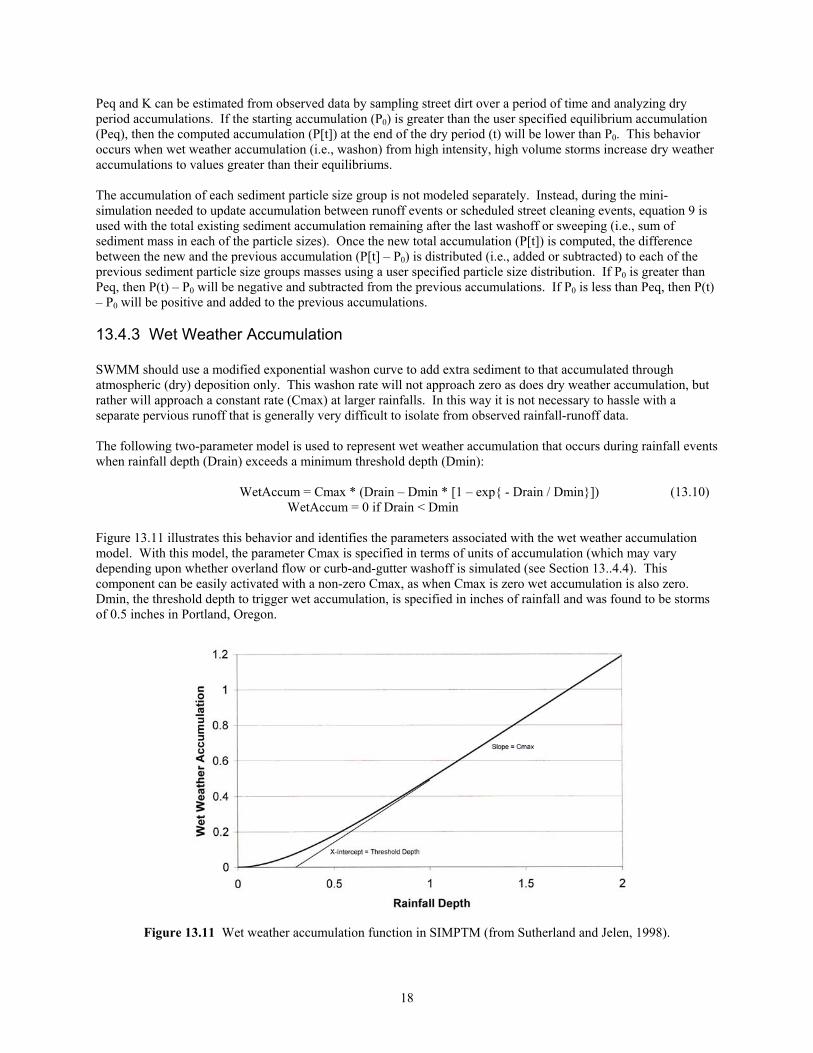
Peq and K can be estimated from observed data by sampling street dirt over a period of time and analyzing dry period accumulations. If the starting accumulation (P0) is greater than the user specified equilibrium accumulation (Peq), then the computed accumulation (P[t]) at the end of the dry period (t) will be lower than P0. This behavior occurs when wet weather accumulation (i.e., washon) from high intensity, high volume storms increase dry weather accumulations to values greater than their equilibriums. The accumulation of each sediment particle size group is not modeled separately. Instead, during the mini-simulation needed to update accumulation between runoff events or scheduled street cleaning events, equation 9 is used with the total existing sediment accumulation remaining after the last washoff or sweeping (i.e., sum of sediment mass in each of the particle sizes). Once the new total accumulation (P[t]) is computed, the difference between the new and the previous accumulation (P[t] – P0) is distributed (i.e., added or subtracted) to each of the previous sediment particle size groups masses using a user specified particle size distribution. If P0 is greater than Peq, then P(t) – P0 will be negative and subtracted from the previous accumulations. If P0 is less than Peq, then P(t) – P0 will be positive and added to the previous accumulations. 13.4.3 Wet Weather Accumulation SWMM should use a modified exponential washon curve to add extra sediment to that accumulated through atmospheric (dry) deposition only. This washon rate will not approach zero as does dry weather accumulation, but rather will approach a constant rate (Cmax) at larger rainfalls. In this way it is not necessary to hassle with a separate pervious runoff that is generally very difficult to isolate from observed rainfall-runoff data. The following two-parameter model is used to represent wet weather accumulation that occurs during rainfall events when rainfall depth (Drain) exceeds a minimum threshold depth (Dmin):

WetAccum = Cmax * (Drain – Dmin * [1 – exp{ - Drain / Dmin}]) (13.10) WetAccum = 0 if Drain < Dmin Figure 13.11 illustrates this behavior and identifies the parameters associated with the wet weather accumulation model. With this model, the parameter Cmax is specified in terms of units of accumulation (which may vary depending upon whether overland flow or curb-and-gutter washoff is simulated (see Section 13..4.4). This component can be easily activated with a non-zero Cmax, as when Cmax is zero wet accumulation is also zero. Dmin, the threshold depth to trigger wet accumulation, is specified in inches of rainfall and was found to be storms of 0.5 inches in Portland, Oregon.

Figure 13.11 Wet weather accumulation function in SIMPTM (from Sutherland and Jelen, 1998).

19

Equation 10 is used to compute a wet weather accumulation whenever the rainfall depth (Drain) from a storm exceeds the minimum threshold depth (Dmin). The wet weather accumulation is then added to the existing accumulation following the washoff simulation for the storm. The wet weather accumulation is distributed based on a user specific particle size distribution for wet weather accumulation. 13.4.4 Impervious Area Washoff The exponential washoff equation being used by SWMM should be retired. The washoff of accumulated sediment from directly connected impervious surfaces is much more complicated than the exponential equation can simulate. In addition, the ability to simulate the effectiveness of source control practices such as street and catchbasin cleaning relies heavily on the accuracy of the washoff simulations that occur for runoff events between cleanings. SWMM should use the same washoff algorithms being used by SIMPTM. Essential to simulating the washoff of suspended solids and other pollutants in urban stormwater is the realization that the process of sediment transport needs to be considered. The recommended washoff algorithms for impervious areas are based on the physical processes of the erosion, transport and deposition (ETD) system described by Curtis (1976). The washoff of sediment from impervious urban areas is a special case of the ETD system in which the available supply of sediment is equal to a reduced amount of particulate material accumulated on the impervious areas. This accumulated particulate material is assumed to be detached, noncohesive, and available for transport. Thus, the detachment processes of rainfall and runoff are not simulated as shown in Figure 13.12. Figure 13.12 taken from Ellis and Sutherland (1979) actually refers to SIMPTM’s predecessor the Particulate Transport Model (PTM) which uses the same washoff equations as SIMPTM. Both models assume that the transport capacity of rainfall is negligible compared to that of runoff.

Figure 13.12 Erosion transport and deposition (EDT) system.

The recommended algorithm uses published sediment transport equations to compute the capacity of either gutter or overland flow (e.g., specified by the user for each impervious surface modeled) to remove various particle sizes of urban sediment (Simons, et. al., 1977 and Foster and Meyer, 1972). At each time step, the current transport capacity is compared to the available sediment supply for each size range to determine which mechanism is controlling the washoff process. If the supply of sediment is greater than the flow’s capacity to transport the sediment, the transport capacity determines the amount of material washed off. If the supply of sediment is less than the flow’s capacity to transport the material, then only the available supply of material is transported. These sediment transport equations are based primarily on an experimentally verified mathematical model developed at Colorado State University (Li, 1974). The researchers applied the work of Einstein, and Meyer-Peter and Muller to an overland flow condition (Einstein, 1950 and Bureau of Reclamation, 1960). The bedload transport equation for gutter flow is based on the Yalin equation as modified by Foster and Meyer to predict transport rates for mixtures of particle sizes (Yalin, 1963).

20

The capacity of shallow flow to transport sediment is largely based upon the physical characteristics of the sediment, notably particle size and specific gravity, and the local hydraulic conditions (e.g., gutter or overland flow). Sediment motion begins when the lift force created by the flow exceeds a critical lift force necessary to lift a particle of sediment off the land surface or bed. The value of the lift force of critical entrainment varies considerably with the particle’s diameter and specific weight. Once a particle has been lifted from the bed material, the drag force of the flow on the particle moves it downstream until changing hydraulic conditions decrease the drag and lift forces to the point that the particle settles to the bed. The lift and drag forces of flow vary with flow depth and velocity. Runoff under steady-state hydraulic conditions has the capacity to transport a certain amount of sediment. The flow transports a greater quantity of the finer particles first. As the supply of these finer particles is depleted, the runoff washes away increasing numbers of the coarser particles, provided the critical lift force of these larger particles has been reached. The washoff algorithm recommended for use by SWMM can simulate the selective nature of sediment transport resulting from either gutter or overland flow. The following assumptions were made in the development of the sediment transport based washoff algorithms:

1. The critical shear force of flow needed to lift a given particle size from the sediment bed is defined by the Shield’s diagram (Vanoni, 1975).

2. Throughout any given time step and along any given flowpath (i.e., gutter or overland):

a. Steady-state hydraulic conditions exist.

b. Average flows are used.

c. The sediment yield for a given particle size range can be approximated by comparing the

sediment availability throughout the entire surface flowpath to the sediment transport capacity computed at a midpoint along the flowpath.

As discussed in Section 13.3.3, only a fraction of the accumulated sediment is available to be washed off. The recommended algorithm correlates the fraction of available accumulated sediment (Sedfrac) to runoff volume (Rundep) up to a user specified maximum fraction (SFmax) achieved at a user specified runoff depth (SFrun) as follows: Sedfrac = SFmax (Rundep / SFrun)2 (13.11) If Rundep > SFrun, Sedfrac = SFmax Calibrations to Bellevue, Washington NURP data resulted in values of 0.15 and 0.04 for the SFmax and SFrun, respectively. So only 15% of the accumulated sediment was available for washoff once the volume of runoff equaled or exceeded 0.04 inches over the entire impervious surface. Bed armoring further limited the available supply of sediment when large stable particles pin and shelter smaller, otherwise unstable particles. Research indicates that it depends upon the composition of the armored bed and the amount of particles already eroded (Vanoni, 1975). The recommended algorithm constantly checks the stability of the largest particle size group with available sediment. When this size group is stable, bed armoring is considered. When only 5% of a group’s accumulation remains during an event, the group can no longer shelter smaller sized groups. The recommended algorithm monitors armoring for each affected size range separately. When armoring occurs at the start of an event, the initially available sediment (P0) is weighted by the proportion of the total bed weight (Ptot) to find the resulting fraction available: Pavail / P0 = ½ P0 / Ptot (13.12)

21

Throughout the remainder of the event, the fraction available in each group relates the remaining available sediment (P) and the initial available sediment: Pavail / P = 1 – P/P0 (13.13) Thus, for a given particle size range, the fraction of sediment currently available for transport will increase as more of its sediment is eroded, an observation by Gessler (Vanoni, 1975). For documentation of the specific washoff equations used by SIMPTM and recommended for use by SWMM, the reader is referred to Sutherland and Jelen (1998). 13.4.5 Pervious Area Washoff Although pervious surfaces usually contribute little to washoff during typical small events, large enough storms can fill the depression storage separating these areas from the drainage system and allow pervious washoff to noticeably contribute to the resulting pollutant loadings. Look outside during an intense rainfall event; fans of soil and debris radiate onto paved streets or parking lots from small adjoining pervious areas which would not pool enough to overflow during smaller events. However, these large deposits often don’t completely washoff but contribute instead to the wet weather accumulation discussed in Section 13.4.3. In an effort to help SWMM isolate pervious area sources of stormwater pollution that contribute directly to washoff during large storms, SWMM should include a simple pervious area washoff equation. The following equation is used by SIMPTM to simulate pervious area sediment washoff (Perwash) and is recommended for use by SWMM: Perwash = Lperv (1 – [1 – Runperv / Dperv]2 ) (13.14) Where Runperv = pervious runoff depth of storm Dperv = pervious runoff depth at which the maximum load is reached Lperv = maximum load per pervious unit area Equation 14, if used, will simulate sediment washoff from pervious areas at a constantly decreasing concentration until a user specified maximum load is realized at a user specified pervious runoff depth. Data collected by the USGS in Madison, Wisconsin (Waschbusch, et. al., 1999) seems to suggest that suspended sediment and associated pollutant concentrations from lawn areas are initially very high with concentrations decreasing with increasing volume. These documents also provide some guidance on the magnitude of the pervious area maximum unit loadings (i.e., Lperv). 13.4.6 Street Cleaning The SWMM street cleaning equation should be replaced by the equation 15 presented below. This equation was originally proposed by Pitt as part of a street cleaning study conducted for the USEPA in San Jose, California (Pitt, 1979). This model was confirmed in additional studies conducted in Alameda County, California (Pitt and Shawley, 1982) and in Washoe County Nevada (Pitt and Sutherland, 1982). These studies found that sweeping removes little, if any, material below a certain base residual which was found to vary by particle size. Above the base residual, the street sweeper’s removal effectiveness was described as a straight line percentage which varied by particle size. For each size group, the amount removed by cleaning (Prem) is related linearly to the initial accumulation (P0) using two parameters – a base residual (SSmin) and a sweeping efficiency (SSeff): Prem = SSeff (P0 – SSmin) for P0 > SSmin (13.15) Therefore, to describe a unique street sweeping operation, one simply needs to know the operations SSmin and SSeff values for each of the ten particle size ranges specified in Section 13.4.1. Note that SSeff is dimensionless, while that for SSmin must match that for accumulation, usually either pounds per curb mile or pounds per paved

22

acre. The initial accumulation (P0) is a simulated parameter, or may be measured in the field (from a similar surface near that swept) in order to evaluate the SSmin and SSeff parameters. If SSmin is zero then the actual pickup efficiency for that cleaning operation and that particle size group is SSeff regardless of the actual accumulation within that size group. High efficiency cleaners exhibit this behavior which makes them extremely effective in removing sediment and pollutants that would have been washed off (Sutherland, et. al., 1998). Please refer to Sutherland and Jelen (1997) for more documentation on equation 15 and the various SSmin and SSeff values estimated for different types of street cleaners. For street cleaning on curbed streets (i.e., curb and gutter washoff hydraulics), one should specify the fraction of curb blocked by parked cars (Park), if any, and thus not swept. SWMM should provide two options associated with the scheduling and simulation of street cleaning. The first is to specify the year, month, day and hour of the first cleaning and the frequency of subsequent cleanings in days. The second option is to provide a specific schedule of the year, month, day and hour of cleanings. If cleaning is scheduled to occur during a runoff event, SWMM should assume that the cleaning will not occur until the next scheduled cleaning time in which runoff is not occurring. 13.4.7 Sediment Trapping Catchbasins SWMM should be able to model the pollutant reduction benefits of using and periodically cleaning sediment trapping catchbasins (STCBs). Very little research has been conducted on the sediment retention effectiveness of sediment trapping inlets or catchbasins. However, experiments by Lager, et. al. (1977) concluded that sediment accumulation in catchbasins is a function of the incoming sediment sizes, the catchbasin volume available to trap sediment, and the runoff flow rate entering the catchbasin. As expected, the larger particles had the highest retention percentage. An initially clean catchbasin can retain up to 45 percent of the incoming sediment (depending on its particle size distribution) until it becomes about half full. The efficiency then quickly drops to zero as the trap fills to approximately 60 percent of the available storage depth. This critical point has been defined as the breakthrough point. The recommended algorithm uses log-log regressions to relate the capture rate for each particle size group (Capfrac) to the retention rate (X), or flow over available trap storage exponentially: Capfrac = ½ (1 – AtrapXBtrap) (13.16) The two-parameter set Atrap and Btrap for each particle size group are coded into the program. The trapping coefficients (i.e., Atrap and Btrap) recommended for use by SWMM were based on a calibration of the SIMPTM model to the extensive Bellevue NURP data set (Sutherland, 1991). 13.5 Closing Remarks The stormwater quality related algorithms currently available in SWMM were presented and discussed. The many problems associated with these algorithms were also presented and discussed. And, finally improvements designed to solve the identified problems were also presented and briefly discussed. The improvements, if implemented, would provide SWMM with the capability to accurately simulate important urban stormwater pollution processes such as accumulation (see Figure 13.13) and washoff (see Figure 13.14). In addition, the improvements would provide SWMM with the ability to estimate the pollutant reduction effectiveness of both street and catchbasin cleaning practices (see Figure 13.15).

23

Figure 13.13 Observed vs simulated street dirt accumulation (from TetraTech/MPS, 2001).

Figure 13.14 Observed vs simulated TSS washoff from downtown commercial site in Portland, Oregon (from Sutherland and Jelen, 1996).

24

Figure 13.15 TSS Washoff reductions for street and catchbasin cleaning (from HRC, 2001).

References Alley, W.M., 1980. Determination of the Decay Coefficient in the Exponential Washoff Equation, Proceedings, International Symposium on Urban Storm Runoff, University of Kentucky, Lexington, Kentucky, pp. 307-311. American Public Works Association, 1969. Water Pollution Aspects of Urban Runoff, U.S. Department of the Interior, Federal Water Pollution Control Administration WP-20-15. Bureau of Reclamation, 1960. Investigation of Meyer-Peter, Muller Bedload Formulas, Sedimentation Section, Hydrology Branch, Division of Project Investigations, U.S. Department of Interior. Curtis, D.C., 1976. A Deterministic Urban Storm Water and Sediment Discharge Model, Proceedings, International Symposium on Urban Hydrology, Hydraulics and Sediment Control, University of Kentucky, Lexington Kentucky. Einstein, H.A., 1950. The Bed Load Function for Sediment Transportation in Open Channel Flows, USDA Technical Bulletin No. 106. Ellis, F.W., and R.C. Sutherland, 1979. An Approach to Urban Pollutant Washoff Modeling, Proceedings, International Symposium on Urban Storm Runoff, Lexington, Kentucky, pp. 325-340. Foster, G.R., and L.D. Meyer, 1972. Transport of Soil Particles by Shallow Flow, Transactions of ASAE, Vol. 15, No. 1. Hubbell, Roth & Clark, Inc., 2001. Storm Sewer Maintenance Study, In association with Pacific Water Resources, Inc., Prepared for the City of Livonia, Michigan. Huber, W.C., and R.E. Dickerson, 1988. Storm Water Management Model User’s Manual, Version 4, U.S. Environmental Protection Agency, Athens, Georgia. Huber, W.C., J.P. Heaney, S.J. Nix, R.E. Dickinson, and D.J. Polmann, 1981. Storm Water Management Model User’s Manual – Version III, U.S. Environmental Protection Agency. Lager, J.A., W.G. Smith and G. Tchobanoglous, 1977. Catchbasin Technology Overview and Assessment, U.S. Environmental Protection Agency, EPA 600/2-77-051.

25

Li, R.M., 1974. Mathematical Modeling of Response from Small Watersheds, Ph.D. Dissertation, Colorado State University, Fort Collins, Colorado. Metcalf and Eddy, Inc., 1971. Storm Water Management Model Volume I – Final Report, U.S. Environmental Protection Agency, 11024DOC07/71. Minton, G., 2002. Guidance on Stormwater Quality Improvement Options for the Snohomish County Drainage Needs Project, Snohomish County, Washington. Pitt, R.E., 1979. Demonstration of Nonpoint Pollution Abatement Through Improved Street Cleaning Practices, U.S. Environmental Protection Agency, EPA 600/2-79-161. Pitt, R.E., 1985. Characterization, Sources and Control of Urban Runoff by Street and Sewerage Cleaning, Contract Number R-80597012, U.S. Environmental Protection Agency, Offices of Research and Development. Pitt, R.E., 1987. Small Storm and Particulate Washoff Contributions to Outfall Discharges, Ph.D. Dissertation, University of Wisconsin, Madison, Wisconsin. Pitt, R.E., and G. Amy, 1973. Toxic Material Analysis of Street Surface Contaminants, U.S. Environmental Protection Agency, EPA-R2-73-283. Pitt, R.E., and J. McLean, 1986. Toronto Area Watershed Management Strategy Study – Humber River Pilot Watershed Project, Ontario Ministry of the Environment, Toronto, Ontario. Pitt, R.E., and G. Shawley, 1982. A demonstration of Nonpoint Pollution Management on Castro Valley Creek, Alameda County Flood Control and Water Conservation District, Hayward, California, prepared for USEPA Water Planning Division. Pitt, R.E., and R.C. Sutherland, 1982. Washoe County Urban Stormwater Management Program – Volume II Street Particulate Data Collection and Analysis, Prepared by CH2M HILL for Washoe Council of Governments, Reno, Nevada. Sartor, J.D., and G.B. Boyd, 1972. Water Pollution Aspects of Street Surface Contaminants, U.S. Environmental Protection Agency, EPA R2-72-081. Simons, D.B., R.M. Li, and T.J. Ward, 1977. A Simple Procedure for Estimating Onsite Soil Erosion, Proceedings, International Symposium on Urban Hydrology, Hydraulics and Sediment Control, University of Kentucky, Lexington, Kentucky, pp. 139-151. Sutherland, R.C., 1991. Modeling of Urban Runoff Quality in Bellevue, Washington, Using SIMPTM, Proceedings, Nonpoint Source Pollution: The Unfinished Agenda for the Protection of our Water Quality, State of Washington, Water Research Center, Report 78. Sutherland, R.C., and S.L. Jelen, 1996. Sophisticated Stormwater Quality Modeling is Worth the Effort, Published in Advances in Modeling the Management of Stormwater Impacts, Volume 4, Edited by William James, CHI Publications, pp. 1-14. Sutherland, R.C., and S.L. Jelen, 1997. Contrary to Conventional Wisdom: Street Sweeping Can be an Effective BMP, Published in Advances in Modeling the Management of Stormwater Impacts, Volume 5, Edited by William James, CHI Publications, pp. 179-190. Sutherland, R.C., and S.L. Jelen, 1998. Simplified Particulate Transport Model User’s Manual, Version 3.2, Pacific Water Resources, Inc., Beaverton, Oregon.

26

Sutherland, R.C., S.L. Jelen, and G. Minton, 1998. High Efficiency Sweeping as an Alternative to the Use of Wet Vaults for Stormwater Treatment, Published in Advances in Modeling the Management of Stormwater Impacts, Volume 6, Edited by William James, CHI Publications, pp. 351-372. Tetra Tech/MPS, 2001. Quantifying the Impact of Catchbasin Cleaning and Street Sweeping on Stormwater Quality for a Great Lakes Tributary: A Pilot Study, Prepared for the Grand River Inter-County Drainage Board, In association with Pacific Water Resources, Inc., Jackson, Michigan. USGS, 1992. Calibration and Users Guide for the Simplified Particulate Transport Model (SIMPTM), Water Resources Division, Austin, Texas. Vanoni, V., ed., 1975. Manual and Report No. 54 – Sedimentation Engineering, American Society of Civil Engineers. Waschbusch, R.J., W.R. Selbig, and R.T. Bannerman, 1999. Sources of Phosphorus in Stormwater and Street Dirt from Two Urban Residential Basins in Madison, Wisconsin, 1994-1995, U.S. Geological Survey, Middleton, Wisconsin, Water Resource Investigations Report 99-4021. Weibel, S.R., R.J. Anderson, and R.L. Woodward, 1964. Urban Land Runoff as a Factor in Stream Pollution, Water Pollution Control Federation Journal, Vol. 36, No. 7. Yalin, M.S., 1963. An Expression for Bed-Load Transportation, Journal Hyd. Div. ASCE, Volume 89, No. HY3, Part I.