STUDIES ON THE RESIDENCE TIME DISTRIBUTION OF SOLIDS IN …

STUDIES ON THE RESIDENCE TIME DISTRIBUTION OF SOLIDS IN A

SWIRLING FLUIDIZED BED

by

AI-IMMAD SHUKRIE BIN MD YUDIN

A Thesis

Submitted to the Postgraduate Studies Programme

as a Requirement for the Degree of

MASTER OF SCIENCE

MECHANICAL ENGINEERING DEPARTMENT

UNIVERSITI TEKNOLOGI PETRONAS

BANDAR SERI ISKANDAR,

PERAK

JUNE 2012

PERPUSTAKAAN UNJVERS;TI MALAYSIA PAl-lANG

No PpeJaq No. Panggilan

Tarikh

2 7 JUL 2612 sg

ABSTRACT

The Multi-Parameter Two-Layer (MPTL) mathematical model was developed in

this work specifically to model the Residence Time Distribution (RTD) of particles in

a continuous system of swirling fluidized bed reactor. The model consists of two

parallel layers. The top layer is a stirred tanks-in-series model and represents the

conventional fluidized bed. Meanwhile, the bottom layer obeys the general recycle

model and represents the swirling motion at the bottom layer of the bed. The Laplace

transformation and convolution integral techniques are used to derive explicit

expressions for the RTD functions of the stirred tanks-in-series model and general

recycle model. The proposed model has six independent parameters - recycle fraction

(P), recycle layer flow rate fraction (w), recycle layer volume fraction (Yr)' number

of tanks in the main flow line of the recycle layer (n1 ), number of tanks in the recycle

line (n2 ) and number of tanks in the top layer (no ). The RTD experiments were

conducted at different particle sizes and bed weights. The bed material used in the

experimental work is spherical plastic beads with a diameter d = 2.99mm

andd = 3.85mm. During hydrodynamics study, it is found that bed pressure drop

AP, increases with air velocity and bed weight. Besides, the smaller bed particle

gives a higher pressure drop for a given bed. The effects of parameters on the RTD

function E(0) are studied and the model is shown to be highly versatile and capable

of representing widely different mixing conditions depending on the system variables.

By best-fitting of the model response to the experimental data, the model parameters

can be evaluated. The experimental result of solid RTD shows that the bed

performance varies from one-layer to two-layer bed as the bed weight increased.

One-layer bed can be modeled by having number of stirred tanks n2 = 4. P, w and

Yr ranging from 0.8 to 0.83, 0.9 to 1.0 and 0.75 to 1.0 respectively. For two-layer

bed, it is found that the combination of n 1 = n2 = n,, = 5 can fit all the runs. The value

vi

of the model parameters P,w and Yr ranging from 0.5 to 0.83, 0.2 to 1.0 and 0.52 to

1.0 respectively.

vii

ABSTRAK

Matematik model yang dipanggil Dwi-Lapisan Pelbagai Pembolehubah

(MPTL) telah dibangunkan dalam penyelidikan mi khusus untuk

menginterpretasikan Pengagihan Masa (RTD) zarah pepejal dalam sistem

berterusan lapisan terbendalir berpusar. Model mi terdiri daripada düa lapisan

selari. Lapisan atas diwakili oleh susunan tanki pengacau dalam kedudukan sesiri

dan ia mewakili lapisan terbendalir konvensional. Sementara itu, lapisan bawah

yang mewakili gerakan berpusar diwakilkan oleh model susunan tangki-pengacau

bagi kitaran yang am. Transformasi Laplace dan teknik Convolution Integral

digunakan untuk memperolehi ungkapan yang jelas untuk fungsi-fungsi

Pengagihan Masa, E(0). Model yang dicadangkan mempunyai enam

pembolehubah bebas - pecahañ kitaran semula (F), pecahan kadar aliran bagi

lapisan kitaran (w), pecahan isipadu bagi lapisan kitaran (Yr)' bilangan tangki-

pengacau di lapisan aliran utama kitaran (n1 ), bilangan tangki-pengacau di lapisan

kitaran (n2 ) dan bilangan tangki-pengacau di lapisan utama (nt ). Eksperimen

bagi menguji Pengagihan Masa zarah di dalam lapisan terbendalir berpusar telah

dijalankan dengan menggunakan saiz dan berat zarah pepejal yang berbeza. Zarah

pepejal yang digunakan di dalam eksperimen mi adalah zarah pepejal sphera yang

masing-masing mempunyai saiz d = 2.99mm dan d = 3.85mm. Semasa kajian

hidrodinamik, didapati bahawa kejatuhan tekanan di dalam sistem lapisan

terbendalir meningkat selari dengan meningkatnya kadar halaju udara yang

disalurkan ke dalam sistem dan juga jurnlah berat zarah pepejal. Selain itu,

kejatuhan tekanan di dalam sistem didapati dipengaruhi oleh saiz zarah pepejal.

Semakin kecil saiz zarah, semakin meningkat kejatuhan tekanan. Kesan parameter

ke atas fungsi Pengagihan Masa E(0) dikaji dan didapati model yang ditunjukkan

mampu mewakili keadaan pencampuran yang berbeza, bergantung kepada

pemboleh ubah sistem. Teknik cuba jaya digunakan untuk menentukan pemboleh

Viii

ubah di dalam matematik model dengan mengubah pemboleh ubah mengikut data

yang diperoleh dad keputusan eksperimen. Keputusan eksperimen Pengagihan

Masa zarah pepejal menunjukkan bahawa, semakin meningkatnya berat zarah

pepejal, lapisan terbendalir didapati berubah-ubah dari satu-lapisan ke dua-

lapisan. Satu-lapisan terbendalir yang direkodkan tersebut boleh dimodelkan oleh

pembolehubah dengan mempunyai bilangan tangki-pengacau sebanyak n 2 =4.

Manakala nilai pemboleh ubah P, w and Yr masing-masing bernilai antara 0.8

hingga 0.83, 0.9 hingga 1.0 dan 0.75 hingga 1.0. Bagi dua-lapisan terbendalir

pula, didapati bahawa kombinasi pembolehubah n1 = n2 = n =5 menepati

eksperimen data dengan sangat baik. Nilai pemboleh ubah model P, w and Yr'

masing-masing didapati berada antara 0.5-0.83, 0.2-1.0 dan 0.52 hingga 1,0.

ix

TABLE OF CONTENTS

STATUS OF THESIS .............................................................................................. 1

APPROVAL PAGE ................................................................................................. ii TITLEPAGE ......................... .................................................................................... DECLARATION ................................................................... . ................................... iv ACKNOWLEDGEMENT............... . ........................... . ............................................. v ABSTRACT............................ . ............................................................................... V

ABSTRAK.................................................................................... viii COPYRIGHT........................................................................................................... TABLEOF CONTENTS ......................... . ............................................................... xi LISTOF TABLES................................................................................................... xiv LISTOF FIGURES ........................................................... . .................... . ................ xv

LISTOF SYMBOLS ............................................................... .. ........................... . .... xviii

Chapter 1. INTRODUCTION

1.1 Introduction ............................................................... 1

1.2 Problem Statements...................................................3

1.3 Objectives ..............................................................4

1.4 Thesis Outline .......................................................... 4

2. LITERATURE RI VIEW 2.1 Introduction .... ...................................... . .................... 5

2.2 Empirical Model for RTD............................................. 7 2.2.1 The Dispersion Model........................................ 7 2.2.2 Stirred Tanks In Series and Parallel Model............... 8 2.2.3 Recycle Model................................................ 10

2.3 Method of RTD Measurement ........................................ 12 2.3.1 Pulse Input ..... ................................................. 13 2.3.2 Step Input;..................................................... 13

2.3.3 Sinusoidal Input ................................................ 13

2.4 Remarks on Earlier Work of RTD .................................... 13

2.5 Summary................................................................ 14

3. METHODOLOGY

3.1 Introduction ................................................................. 23

3.2 Proposed Multi-Parameter Two Layer (MPTL) Model...........23

3.2.1 Physical . Representation of the Bed Behavior by the MPTLModel...................................................25

3.2.2 Development of the MPTL Model..........................37 3.2.3 RTD Density Function.......................................31

xl

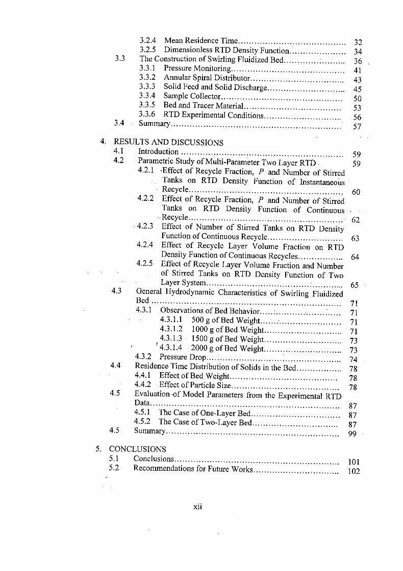
3.2.4 Mean Residence Time ......................................... 32 3.2.5 Dimensionless RTD Density Function ...................... 34

3.3 The Construction of Swirling Fluidized Bed .............. . ......... 36 3.3.1 Pressure Monitoring.......................................... 41 3.3.2 Annular Spiral Distributor................................... 43 3.3.3 Solid Feed and Solid Discharge3.3.4

.............................Sample Collector

45

3.3.5................... . .........................

Bed and Tracer Material50 53

3.3.6....................................

RTD Experimental Conditions ............................. 56 3.4 Summary................................................................ 57

4. RESULTS AND DISCUSSIONS

4.1 Introduction ............................................................

4.2 Parametric Study of Multi-Parameter Two Layer RID 59 4.2.1 -Effect of Recycle Fraction, P and Number of Stirred

Tanks on RTD Density Function of Instantaneous • Recycle ............................................................ 60

4.2.2 Effect of Recycle Fraction, P and Number of Stirred Tanks on RTD Density Function of Continuous

• Recycle ........................................................... 62 4.2.3 Effect of Number of Stirred Tanks on RTD Density

Function of Continuous Recycle ............................ 63 4.2.4 Effect of Recycle Layer Volume Fraction on RTD

Density Function of Continuous Recycles................. 64 4.2.5 Effect of Recycle Layer Volume Fraction and Number

of Stirred Tanks on RTD Density Function of Two LayerSystem.................................................... 65

4.3 General Hydrodynamic Characteristics of Swirling Fluidized Bed.....................................................................4.3.1 Observations of Bed Behavior .................................

71 71

4.3.1.1 500gof Bed Weight .... .. ........................... 71 4.3.1.2 l000gof Bed Weight ............................. 71 4.3.1.3 l500gof Bed Weight ............................. 73 4.3.1.4 2000 g of Bed Weight............................. 73

4.3.2 Pressure Drop ................................................... 74 4.4 Residence Time Distribution of Solids in the Bed ................. 78

4.4.1 Effect, of Bed Weight........................................ 78 4.4.2 Effect of Particle Size 78 ........................................ .

4.5 Evaluation of Model Parameters from the Experimental RID Data...................................................................... 4.5.1 The Case of One-Layer Bed

87 .................................

4.5.2 The Case of Two-Layer Bed................................87 87

4.5 Summary ................................................................ 99

5. CONCLUSIONS

5.1 Conclusions ............................................................. 101

5.2 Recommendations for Future Works................................102

xii

REFERENCES

103

APPENDIXES A Convolution Integral of RTD Density Function 109 B RTD Experimental Procedures 118

xiii

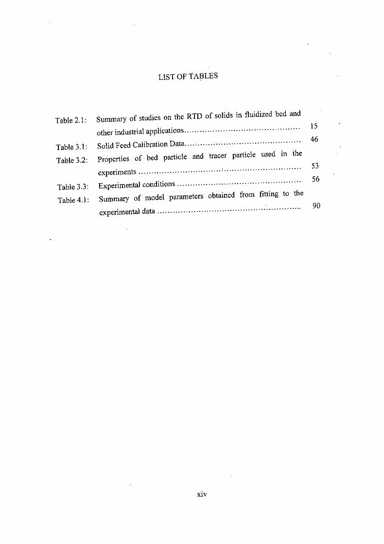
LIST OF TABLES

Table 2.1: Summary of studies on the RTD of solids in fluidized bed and

other industrial applications.............................................

Table 3.1: Solid Feed Calibration Data.............................................

Table 3.2: Properties of bed particle and tracer particle used in the

experiments...............................................................

Table 3.3: Experimental conditions ................................................

Table 4.1: Summary of model parameters obtained from fitting to the

experimental data ........................................................

15

46

53

56

xiv

LIST OF FIGURES

Figure 1.1: Schematic of Two Layer Bed .................................... 3

Figure 2.1: Stirred tanks in series model ..................................... 9

Figure 2.2: Stirred tanks in series and parallel model ...................... 9

Figure 3.1: Flow chart of research methodology ........................... 24

Figure 3.2: Physical observation from the operation of swirling

fluidized bed ..........................................................' 25

Figure 3.3: Schematic of Two Layer Bed ..................................... 26

Figure 3.4: Multi Parameter Two Layer Model ............................ 26

Figure 3.5: Schematic of the experimental apparatus ...................... 38

Figure 3.6: Photograph of experimental apparatus of Swirling

Fluidized Bed ...................................................... 39

Figure 3.7: Close-up view of experimental apparatus of Swirling

Fluidized Bed ...................................................... 40

Figure 3.8: Photograph of Swirling Fluidized Bed with metal cone and

pressuretaps ......................................................... 42

Figure 3.9: Photograph of arrangement of annular distributor ............ 43

Figure 3.10 Photographs of close view arrangement of annular

distributor .......................................................... 44

Figure 3.11: Solid feed performance curve ................................... 46

Figure 3.12: Photographs of feeder hopper ................................... 47

Figure 3.13: Close view photograph of feeder hopper connected with

salt-and-dispenser mechanism gate valve ..................... 48

Figure 3.14: Close view photographs of salt-and-dispenser mechanism

gatevalve ........................................................... 49

Figure 3.15: Photograph of sample collector ................................. 50

Figure 3.16 (a): Photograph of sample collector assembly ...................... 51

Figure 3.16 (b): Close view photograph of ball-bearing and slot mechanism 51

Figure 3.17: Schematic drawing ofsample collector ........................ 52

xv

Figure 3.18: Photograph of 3.85 mm white particles....................... 54

Figure 3.19: Photograph of 2.99 mm cream particles...................... 54

Figure 3.20: Photograph of 3.85 mm blue particles........................ 55

Figure 3.21: Photograph of 2.98 mm. dark blue particles.................. 55

Figure 4.1: Effect of recycle fraction on RTD density function of

instantaneous recycles ............................................ 61

Figure 4.2: Effect of number of stirred tanks in main flow line on RTD

density function of instantaneous recycle ...................... 62

Figure 4.3: Effect of recycle fraction on RTD density function of

continuous recycle ................................................ 63

Figure 4.4: Effect of number of stirred tanks in main flow line on RTD

density function of continuous recycle ...................... 64

Figure 4.5: Effect of recycle layer volume fraction on RTD density

function of two layer bed at w0.5 ............................. 65


function of two layer bed at = 0.2 ............................ 66


function of two layer bed at w = 0.5 ............................ 67


function of two layer bed at w = 0.9 ............................ 68

Figure 4.9: Effect of number of stirred tanks, n = n, = n2 = 10 and

recycle layer volume fraction on RTD density function of69

two layer bed at w0.2 ..........................................

Figure 4.10: Effect of number of stirred tanks, n = n1 = n2 =20 and

recycle layer volume fraction on RTD density function of70

two layer bed atWO.2 ..........................................

Figure 4.11:Observation of slugging motion during hydrodynamics 72 study of swirling fluidized bed...................................

Figure 4.12: Bed pressure drop vs. superficial air velocity for 2.99 mm

spherical particles ................................................75

Figure 4.13: Bed pressure drop vs. superficial air velocity for 3.85mm

spherical particles ................................................76

xvi

Figure 4.14: Comparison of bed pressure drop vs. superficial air velocity

for two particle sizes .................................... 77

Figure 4.15: RTD density function of 2.99 mm particle at 500 g .......... 79

Figure 4.16: RTD density function of 2.99 mm particle at 1000 g ......... 80



Figure 4.19: RTD density function of 3.85 mm particle at 500 g ..........83

Figure 4.20: RID density function of 3.85 mm particle at 1000 g ......... 84



Figure 4.23: Fitting of MPTL model to experimental data for RTD

density function of 2.99 mm particle at 500 g ................ 91

Figure 4.24: Fitting of MPTL model to experimental data for RID

density function of 2.99 mm particle at 1000 g ............... 92

Figure 4.25: Fitting of MPIL model to experimental data for RTD





density function of 3.85 mm particle at 500 g ................. 95





Figure 4.30: Fitting of MPTL model to experimental data for RID


xvii

NOMENCLATURE

d inner diameter of the distributor [mm]

d0 outer diameter of the distributor [mm]

d particle diameter [mm]

E(t) residence time distribution density function [s']

E(s) transfer function [-1

E(0) dimensionless residence time distribution density [-1

function

hmj bed height at minimum fluidization [mm]

static bed height [mm]

Mb total bed weight [g]

MbS stagnant bed weight [g]

MT total tracer weight added to the bed [g]

M 1 tracer weight in sample no. i [g]

NOB number of distributor blades

total number of samples collected in each experiment

n number of stirred tanks-in-series

P recycle fraction [-]

static bed pressure [mmH20]

AP, bed pressure drop [mmH20]

AP total pressure drop [mml-120]

Q flow rate [m3/h]

Qa ar flow rate [m 3/h]

Q solid flow rate [m 3/h]

S variable of Laplace Transformation [-]

xviii

AT sampling period [s]

t residence time [s]

mean residence time [s]

th mean holding time [s]

t i clock time of sample no. i [s]

U superficial air velocity [m/s]

U,, horizontal component of air velocity [m/s]

• U, initial fluidization velocity [m/s]

minimum fluidization velocity [m/s]

U, minimum swirling velocity [m/s]

vertical component of air velocity [m/s]

minimum slugging velocity [m/s]

u minimum two-layer velocity [m/s]

V volume [m3]

W recycle layer volume fraction

Y main flow line volume fraction

Yr recycle layer volume fraction

SUPERSCRIPTS

* denotes convolution integral

* m denotes rn-fold convolution integral

xix

SUBSCRIPTS

denotes main flow line

2 denotes recycle line

n denotes individual stirred tank

o denotes total

p denotes top layer

denotes bottom recycle layer

ABBREVIATIONS

MPTL multi-parameter-two-layer

RT residence time

RTD residence time distribution

xx

CHAPTER 1

INTRODUCTION

1.1 Introduction

Fluidized bed technology has been utilized in chemical, petroleum, mineral

processing and other industrial processes since its advent during World War II.

Applications of this technology include: particle processing such as cooling, heating,

roasting, drying, coating, granulation and transportation, cracking and reforming of

hydrocarbons, coal carbonization and gasification, Fischer-Tropsch synthesis etc. In

spite of its importance and wide application, knowledge of basic fluidization

phenomena is still very rudimentary and the design of fluidized bed reactors is, at

best, difficult, imprecise, and based mainly on experience on know-how. This is

because the flow behavior of fluidized bed is sensitive to bed geometry, scale and

operating conditions.

Although a number of fluidized bed reactor models have appeared in

literature, it is still difficult to identify which one of these models represents the

fluidized bed behavior most closely for a given application. Fluidized bed reactors

have gained wide use because of a number of highly useful properties, the most being

concerned with their excellent heat transfer characteristics and temperature control,

continuity of operation, efficient handling of large quantities of solids and excellent

fluid-solid contact. Gas fluidized bed technology is increasingly being applied to a

wide range of industrial applications where good mixing and/or heat transfer must be

achieved.

1

There have been many efforts to expand fluidized bed performance and to

have different varieties of its operation. Different designs of the distributors and a

study of the effect resulting from bed-distributor interaction on bed performance,

extensive studies of bubble characteristics and studies of internals location, position

and configuration in the gas fluidized bed are examples of attempts at understanding

and improving the bed performance. The circulating fluidized bed is one variant of

fluidized bed which has assumed considerable importance especially in combustion

applications. Tapered fluidized bed and centrifugal fluidized bed are other variants of

fluidized bed which have been proposed to overcome certain limitations of the

conventional fluidized bed.

One of the promising candidates is a swirling fluidized bed which could be of

many designs to impart swirling motion to the bed particles. In the present work, a

variant of continuous fluidized bed that features an annular bed, angular injection of

gas through the distributor blades and swirling motion of bed material in a confined

circular path is introduced and studied. When a jet of gas enters the bed at an angle 0

to the horizontal, the gas velocity U will have two components; the vertical

component, U, = U sin responsible for fluidization and causes lifting of particles

and, the horizontal component Uh = U cos 0 creates a swirling motion of the particles

[1], [2]. The gas entering the bed will impart a tangential motion to the particles and

will progressively turn to a vertical direction of flow. Thus, at successive layers of the

bed, the tangential component of particle motion will decay with bed height. In the

general case, one may visualize a bed with a lower swirling layer and an upper non-

swirling conventional layer (Fig. 1 .1).

2

Top Conventional

Layer

Bottom Swirling Layer

Fig. 1.1 Schematic of Two Layer Bed.

From the visual observation of the swirling fluidized bed during operation, as the

air velocity increases, the sequence of flow regimes observed are packed bed, partially

fluidized bed and wave motion regime. On further increase of the air velocity,

particles at the top layer of the bed are fully fluidized and the bed is bubbling.

Meanwhile, the particles at the bottom layer of the bed are in swirling motion. This is

the regime of the two layer fluidized bed. The velocity is termed as the minimum

two-layer velocity, U,. As the air velocity increases further, the height of swirling

layer increases until it dominates the entire bed and the bed become a single swirling

mass.

1.2 Problems Statements

In continuous processing of solids in a fluidized bed, it is necessary to have

quantitative information on the residence time distribution (RTD) of solids in the bed,

which is fundamental to the design, study and analysis of the system performance.

The RTD approach is utilized to gain knowledge of the overall system dynamics since

single particle dynamics and accurate description of its history in the bed are difficult.

This thesis presents an analytical and experimental study of the RTD of solids in

continuous swirling fluidized bed.

3

1.3 Objectives

The objectives of the present works are:

a.To propose a general RTD model which achieves both physical representation

of the bed behavior and an accurate fit to the experimental data through

adequate flexibility of the model.

b. To perform detailed experimental study of particles in the swirling fluidized

bed covering a wide range of variables, viz., bed height, bed weight, gas

velocity and particle size.

C.

To conduct comparative analysis of the experimental data and the RTD model,

by best-fitting of the model response to the experimental data, to evaluate the

model parameters.

1.4 Thesis Outline

This thesis consists of 5 chapters. The first chapter sets out the context against this

research was carried out, the objectives of the present research and an outline

structure of the thesis. Since this research work required a current working knowledge

of RTD, their relevant literatures were reviewed respectively in Chapter 2.

Multi-Parameter Two-Layer (MPTL) Residence Time Distribution RTD

model was introduced in Chapter 3. The model is developed based on the observation

of bed that exhibits two-layer during the operation. Continuous Stirred Tanks Reactor

(CSTR) in-series were used to model the MPTL in swirling fluidized bed. Besides,

experimental procedure and development of experimental rigs are explained in details

in Chapter 3.

Parametric analysis of MPTL model and experimental investigations are

presented in Chapter 4. The present findings are analyzed and discussed. Finally

conclusions and recommendations for future research are formulated in Chapter 5.

4

CHAPTER 2

LITERATURE REVIEW

2.1 Introduction

The measurement and accurate analysis of residence time distribution (RTD) has

become a prominent tool in the study, analysis and design of continuous flow

systems, for evaluating the performance of a continuous fluidized bed and to gain an

insight into the fluid process. Residence time theory deals with how particles enter,

flow through and leave a system. Intuitively it seems natural to expect that not all the

particles will have the same residence time. The idea of using the distribution of

residence times in the analysis of chemical reactor was first proposed in a pioneering

paper by Danckwerts [3] in 1953 where he used the internal and exit age distributions

to characterize the residence time distributions in a system.

RTD can be measured directly by a widely used method of inquiry, the

stimulus response experiment, which is based on the introduction of some tracer

(stimulus) and measurement of the time independence of the tracer in the outflow

(response) [4]. Four different injection techniques of tracer are used, pulse, step,

periodic concentration fluctuation or random concentration change. The pulse and

step input of tracer are easier to interpret. Therefore, they are the most widely used

techniques [5], [6].

From a pulse injection, the residence time distribution density function

E(t) introduced by Danckwerts [3] is defined such that E(t)dt is the fraction of the

fluid that spends a given duration, t inside the reactor and has the unit of s'.

= (2.1)

5

Another function capable of characterizing RTD is F curve. The F curve is the

integral of exit age distribution function, E(t);

F(t) = JE(t)dt (2.2)

In many cases a dimensionless time 0 is a better time parameter than t. The

dimensionless time 0 is defined as 9 = where I is a mean residence time or mean t

holding time. A great deal of literature attention has been devoted to determine I

from physical considerations. For a constant density system, Levenspiel [7] showed

that I = - where V is the volume of the system and Q is the volumetric flow rate.

This result of I was part of a more general theorem that relates Ito the ratio of total

particle inventory (or hold up of particles in the system) to total throughput (total

outflow of particle). The mean residence time I and the variance of RTD can also be

obtained from the relations;

(2.3) 1=

It has become standard practice to discuss RTD and its models in their

dimensionless or normalized forms so that t is not considered an adjustable parameter

in the models. The normalized form of RTD functions are:

E(9) = IE(t) = IE(I0)- dF(0) (2.4)

- dO

(2.5) F(0) = F(t) = fE(0)dO = F(IO)

Another important property of the RTD function is the convolution integral

theorem discussed in detailed by Levenspiel [7] and being used by Mann et al. [8] and

Fu et al. [9]. The convolution integral relates the shapes of the initial tracer

disturbance with the shape of the final exit age distribution curve. The

simplestexample of a convolution integral is obtained when two reactors are

connected in series and the RTD over the two reactors is measured. The final RTD is

equal to the RTD in the first reactor convoluted in the second one. The mathematical

expression is described in integral form as:

E1 *2 (t) = E1 (t) *E1 Q) = fE, El (t — -r)dr

(2.6)

Non-ideal flow within the continuous systems can be characterized by using

few RTD models available in the literature. All the models take the form of

mathematical functions which describe the curves E(0) and F(0). All models for

RTD of solids in a continuous fluidized bed are Empirical models which have one or

more adjustable parameters.

2.2 Empirical Model for RTD

Empirical models can be classified in different ways. They can be classified based on

their mathematical description and basic assumption given by Varma [10] or on the

basis of number of parameters on the model done by Levenspiel [7], which will be the

basis used in this study.

2.2.1 The Dispersion Model

The dispersion model assumes a uniform velocity for the solids over the cross section,

with some degree of back mixing super-imposed on it which is uniquely characterized

by a longitudinal axial dispersion coefficient (P,,). The dispersion model is based on

the equation

aCD,a2c ac ao ( (2.7)

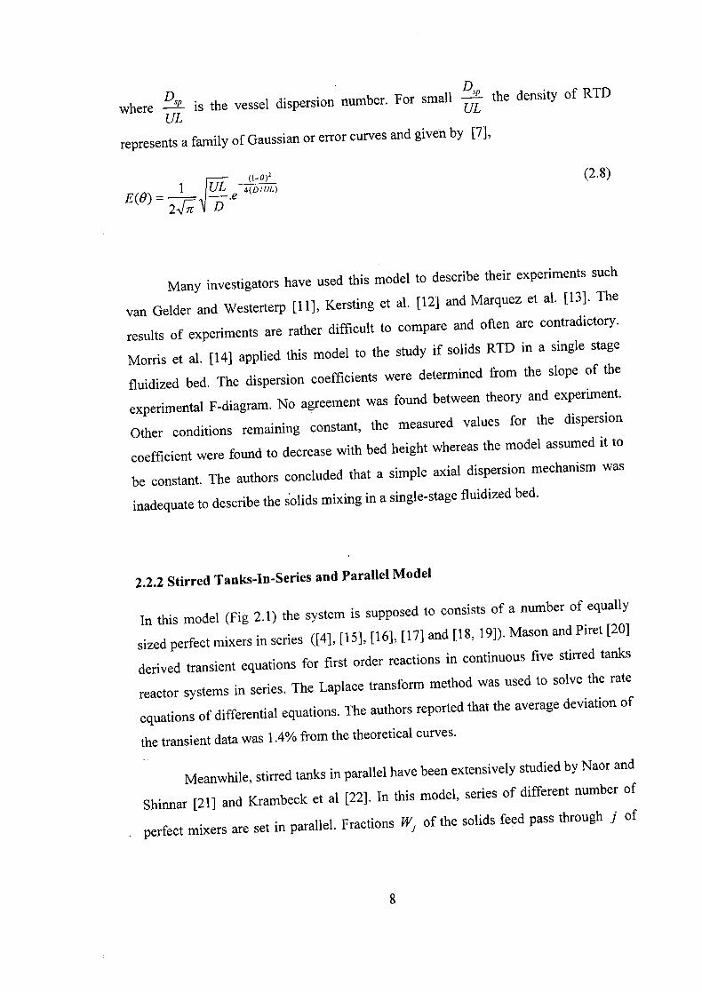
D where -- is the vessel dispersion number. For small -- the density of RTD UL

UL

represents a family of Gaussian or error curves and given by [7],

1 4(D/UL) 2 FD E(0) =

Many investigators have used this model to describe their experiments such

van Gelder and WesterterP [11], Kersting et al. [12] and Marquez et al. [13]. The

results of experiments are rather difficult to compare and often are contradictory.

Morris et al. [141 applied this model to the study if solids RTD in a single stage

fluidized bed. The dispersion coefficients were determined from the slope of the

experimental F-diagram. No agreement was found between theory and experiment.

Other conditions remaining constant, the measured values for the dispersion

coefficient were found to decrease with bed height whereas the model assumed it to

be constant. The authors concluded that a simple axial dispersion mechanism was

inadequate to describe the Solids mixing in a single-stage fluidized bed.

2.2.2 Stirred Tanks-In-Series and Parallel Model

In this model (Fig 2.1) the system is supposed to consists of a number of equally

sized perfect mixers in series ([4], [ 15 ], [161, [171 and [18, 19]). Mason and Piret [20]

derived transient equations for first order reactions in continuous five stirred tanks

reactor systems in series. The Laplace transform method was used to solve the rate

equations of differential equations. The authors reported that the average deviation of

the transient data was 1.4% from the theoretical curves.

Meanwhile, stirred tanks in parallel have been extensively studied by Naor and

Shinnar [21] and Krambeck et al [22]. In this model, series of different number of

perfect mixers are set in parallel. Fractions Wj of the solids feed pass through j of

(2.8)

8

the parallel series which has n equally sized perfect mixers as shown in Fig. 2.2.

Then the RTD function is given by

F(0) =1— Wmie'°J1

(2.9)

where m total number of parallel paths.

Direction of fluid flow

Stirred tanks Stirred tanks

Fig. 2.1 Stirred tanks in series model.

Wmj 0J0

Stirred tanks

Total flow rate Qo Wj

Direction of Stirred tanksfluid flow

Wi * Lni

Stirred tanks

Fig. 2.2 Stirred tanks in series and parallel model.

Documents

STUDIES ON THE RESIDENCE TIME DISTRIBUTION OF SOLIDS IN …