T R A I N I N G C O U R S E S E R I E S 31

Radiotracer ResidenceTime Distribution Method

for Industrial andEnvironmental Applications

Material for Education and On-the-Job Training forPractitioners of Radiotracer Technology

V I E N N A , 2 0 0 8

TRAINING COURSE SERIES No. 31

Radiotracer Residence Time Distribution Method

for Industrial and Environmental Applications

Material for Education and On-the-Job Training for Practitioners of Radiotracer Technology

INTERNATIONAL ATOMIC ENERGY AGENCY, VIENNA, 2008

The originating Section of this publication in the IAEA was:

Division for Asia and the Pacific International Atomic Energy Agency

Wagramer Strasse 5 P.O. Box 100

A-1400 Vienna, Austria

RADIOTRACER RESIDENCE TIME DISTRIBUTION METHOD FOR INDUSTRIAL AND ENVIRONMENTAL APPLICATIONS

IAEA-TCS-31 ISSN 1018–5518

© IAEA, 2008

Printed by the IAEA in Austria

May 2008

IAEA, VIENNA, 2008

FOREWORD

The International Atomic Energy Agency (IAEA) plays a major role in facilitating the transfer

of the radiotracer technology to developing Member States. The major radiotracer techniques have been implemented through IAEA technical cooperation projects and adopted by many Member States. The expertise and knowledge gained should be preserved. The sustainability of technology and knowledge preservation calls for creation of young specialists and for continuing good practices.

As a part of its involvement in human resource development, the IAEA is aware of the

important need to prepare standard syllabi and training course materials for the education of specialists in different fields of nuclear technologies. This training course material is intended for the cultivation of radiotracer specialists and for continuing technical education of radiotracer practitioners worldwide. The wide interest in radiotracer technology has created the need for high level professional education and training in this field, which are not necessarily covered by traditional university courses.

Radiotracers are playing more and more important roles in industry. These roles will continue to

expand, especially if students and engineers are exposed in their academic training to the many possibilities for using this tool in research, development and applications. Besides educational purposes, this publication will assist developing Member States in establishing their quality control and accreditation systems.

This publication is based on lecture notes and practical works delivered by many experts in

IAEA-supported activities. Lectures, papers, case studies and software were reviewed by a number of specialists in several meetings. In particular, S. Charlton, S.H. Jung, I.H. Khan, H.J. Pant and P. Zhang have provided substantial technical inputs. The IAEA wishes to thank all the specialists for their valuable contributions.

The IAEA officers responsible for this publication are P.M. Dias of the Department of

Technical Cooperation, and Joon-Ha Jin of the Division of Physical and Chemical Sciences.

EDITORIAL NOTE

The use of particular designations of countries or territories does not imply any judgement by the publisher, the IAEA, as to the legal status of such countries or territories, of their authorities and institutions or of the delimitation of their boundaries.

The mention of names of specific companies or products (whether or not indicated as registered) does not imply any intention to infringe proprietary rights, nor should it be construed as an endorsement or recommendation on the part of the IAEA.

CONTENTS

INTRODUCTION....................................................................................................................................1

1. ELEMENTS OF RADIATION PHYSICS ..........................................................................................2

1.1. Radiation and radioisotopes ..........................................................................................................2 1.1.1. Structure of the atom............................................................................................................2 1.1.2. Alpha, beta and gamma........................................................................................................3 1.1.3. Neutrons ...............................................................................................................................6 1.1.4. Radioactive decay and half-life............................................................................................6

1.2. Radiation units ..............................................................................................................................8 1.2.1. Unit of radioactivity .............................................................................................................7 1.2.2. Dose units.............................................................................................................................8 1.2.3. Radiation dose rate in the vicinity of a point source of gamma rays ...................................8

1.3. Radiation detection .......................................................................................................................9 1.3.1. Gas filled radiation detectors ...............................................................................................9 1.3.2. Scintillation radiation detectors..........................................................................................10 1.3.3. Semiconductor (solid state) detectors ................................................................................10 1.3.4. Detector efficiency.............................................................................................................11

1.4. Radiation protection and safety...................................................................................................12 1.4.1. ALARA principle...............................................................................................................12 1.4.2. Radiation safety considerations in radiotracer applications...............................................12

2. RADIOACTIVE TRACERS..............................................................................................................13

2.1. Types of tracers...........................................................................................................................13 2.1.1. Intrinsic and extrinsic tracers .............................................................................................14

2.2. Advantages of radiotracers..........................................................................................................15 2.3. Selection of a radiotracer ............................................................................................................16 2.4. Methods and techniques for labelling .........................................................................................17

2.4.1. Solid materials....................................................................................................................17 2.4.2. Aqueous systems................................................................................................................20 2.4.3. Organic materials ...............................................................................................................20 2.4.4. Gaseous materials ..............................................................................................................21

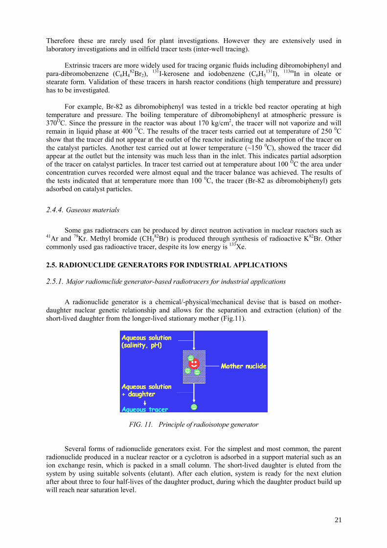
2.5. Radionuclide generators for industrial applications....................................................................21 2.5.1. Major radionuclide generator-based radiotracers for industrial applications.....................21 2.5.2. Application of radionuclide generator-based radiotracers .................................................23

2.6. Mixing length estimation ...........................................................................................................25 2.6.1. Definition of mixing length................................................................................................25 2.6.2. Examples of injection techniques for reducing mixing length...........................................26

3. RADIOTRACER DETECTION ........................................................................................................28

3.1. On-line and off-line measurements.............................................................................................28 3.2. On-line measurements using gamma radiotracers ......................................................................28

3.2.1. Influence ofd various parameters .......................................................................................28 3.2.2. Data acquisition..................................................................................................................31

3.3. Off-line measurements................................................................................................................33 3.3.1. Sampling measurement ......................................................................................................33

4. FORMULATION OF THE RESIDENCE TIME DISTRIBUTION .................................................35

4.1. Residence time distribution (RTD) measurement.......................................................................35 4.2. RTD formulation.........................................................................................................................36

4.2.1. Dead time correction..........................................................................................................37 4.2.2. Background correction .......................................................................................................37 4.2.3. Radioactive decay correction .............................................................................................37 4.2.4. Filtering (or smoothing) .....................................................................................................38 4.2.5. Data extrapolation ..............................................................................................................39

4.2.6. Normalization of the area of experimental tracer curve.....................................................39

5. RTD TREATMENT AND MODELING...........................................................................................40

5.1. Calculation of moments ..............................................................................................................40 5.2. RTD system analysis...................................................................................................................41

5.2.1. Methodology ......................................................................................................................41 5.2.2. Elementary models.............................................................................................................42 5.2.3. Models for non-ideal flows ................................................................................................43 5.2.4. Rules for combining simple models...................................................................................47 5.2.5. Optimization procedure — Curve fitting method ..............................................................48 5.2.6. Example of simple modelling: Mixer cascade with three compartments ..........................49

5.3. Convolution and deconvolution procedures................................................................................51 5.3.1. Convolution........................................................................................................................51 5.3.2. Deconvolution....................................................................................................................53

6. PLANNING AND EXECUTION OF A RADIOTRACER EXPERIMENT ....................................53

6.1. Amount of activity ......................................................................................................................53 6.1.1. Factors influencing the radiotracer activity........................................................................53 6.1.2. Estimation of radiotracer activity for RTD tests ................................................................54

6.2. Implementation of the RTD test..................................................................................................55

7. RESIDENCE TIME DISTRIBUTION APPLICATIONS.................................................................57

7.1. Major targets ...............................................................................................................................57 7.2. RTD for troubleshooting.............................................................................................................58

7.2.1. Dead/stagnant volume........................................................................................................60 7.2.2. Bypassing/channelling .......................................................................................................60

7.3. RTD for diagnosis of industrial processes: Case studies ............................................................61 7.3.1. Radiotracers for diagnosis of fluid catalytic cracking (F.C.C.) units.................................61 7.3.2. Liquid flow in trickle bed reactors .....................................................................................64 7.3.3. RTD to solve the problem of fluid maldistribution within a packed bed tower.................68 7.3.4. Radioatracer investigation of pulp flow dynamics in a phosphate chemical reactor .........71 7.3.5. Diagnosis of leaching and flotation processes ...................................................................75 7.3.6. Heavy metal release in a pilot plant scale municipal solid waste incinerator ....................80 7.3.7. Gas flow distribution in a SO2 — Oxidation industrial reactor..........................................83 7.3.8. Improvement of a grinding process....................................................................................85 7.3.9. Investigation of cobalt recovery and mass flow dynamics in a

copper melting process ......................................................................................................86 7.3.10. Estimation of laterite grain erosion in a fluidised bed calciner........................................88 7.3.11. Radiotracer valuation of coal-ash dust cyclone efficiency...............................................89 7.3.12. RTD for diagnosing a concrete mixing machine .............................................................90 7.3.13. Radiotracer for efficiency evaluation of irradiation chamber for flue gas treatment .......91 7.3.14. Radiotracer investigations of wastewater treatment plants ..............................................94 7.3.15. Radiotracers for flow meter calibration .........................................................................109 7.3.16. Interwell tracer technique (IWTT) .................................................................................111

8. RTD SOFTWARE FOR MODELING SIMPLE FLOWS...............................................................117

8.1. A manual for the RTD software................................................................................................117 8.1.1. Introduction: What does it do?.........................................................................................117 8.1.2. Data input — Preparing the calculation ...........................................................................117 8.1.3. Running the calculation, seeing the results ......................................................................120

8.2. Description of models available in the RTD software ..............................................................123 8.2.1. Axial dispersed plug flow ................................................................................................123 8.2.2. Axial dispersed plug flow with exchange ........................................................................123 8.2.3. Perfect mixers in series ....................................................................................................124 8.2.4. Perfect mixers in series with exchange ............................................................................124 8.2.5. Perfect mixers in parallel .................................................................................................125

8.2.6. Perfect mixers with recycle..............................................................................................125 8.3. Purpose of tutorials ...................................................................................................................125

8.3.1. Tutorial to CASE 1 ..........................................................................................................126 8.3.2. Tutorial to CASE 2 ..........................................................................................................127 8.3.3. Tutorial to CASE 3 ..........................................................................................................128 8.3.4. Tutorial to CASE 4 ..........................................................................................................129 8.3.5. Case study exercise: Model of water flow by gravity through two tanks in series ..........131

9. LABORATORY WORKS ...............................................................................................................133

9.1. Closed circuit water flow rig for laboratory RTD tests.............................................................133 9.1.1. Flow rig experimental setup.............................................................................................133 9.1.2. Some examples of radiotracer tests performed in the flow rig ........................................134

9.2. Laboratory Work 1: Determination and analysis of RTD in process vessels ...........................136 9.2.1. Theory ..............................................................................................................................136 9.2.2. Part A: Determination of the residence time distribution (RTD).....................................137 9.2.3. Part B: Parameter estimation by time-domain curve fitting.............................................138 9.2.4. Part C: Parameter estimation by the method of moments ................................................138

9.3. Laboratory Work 2: Detection of dead space and channelling .................................................139 9.3.1. Theory ..............................................................................................................................139 9.3.2. Part A: Detection of dead space .......................................................................................140 9.3.3. Part B: Detection of channelling (Bypassing)..................................................................141

9.4. Laboratory Work 3: RTD curves and parameter estimation in combined model systems........141 9.4.1. Theory ..............................................................................................................................141 9.4.2. Part A: Stirred tank in series with plug flow....................................................................143 9.4.3. Part B: Tanks in parallel...................................................................................................144

10. QUESTIONS ON RTD METHODOLOGY AND TECHNOLOGY ............................................144

BIBLIOGRAPHY ................................................................................................................................149

CONTRIBUTORS TO DRAFTING AND REVIEW..........................................................................153

INTRODUCTION

The concept of residence time distribution (RTD) has become an important tool for the analysis

of industrial units and reactors. The RTD of fluid flow in process equipment determines their performance. Radiotracers are method of choice for obtaining the RTD in industrial processing vessels and wastewater treatment systems. Radiotracer RTD method has been extensively used in industry to optimize processes, solve problems, improve product quality, save energy and reduce pollution. The technical, economic and environmental benefits have been well demonstrated and recognized by the industrial and environmental sectors. Though the RTD technology is applicable across a broad industrial spectrum, the petroleum and petrochemical industries, mineral processing and wastewater treatment sectors are identified as the most appropriate target beneficiaries. These industries are widespread internationally and are of considerable economic and environmental importance.

There is little experience in teaching the use of radiotracers, and the available books on this

subject are either application or principle oriented. This text is the result of the belief that there is a need to develop radiotracer RTD measurement applications from fundamental principles. The theoretical treatment is applied to the extent possible, but, when complete analytical treatments are not practical, a mechanistic or phenomenological approach is adopted. Although many applications are included as illustrations, this is not intended as a bibliography of applications. The application illustrations chosen represent the major problems of industry where the radiotracer RTD method is very competitive.

This training course material is organized into ten sections. The characteristics of nuclear

radiation are described in section one on elements of radiation physics. Radiation and radioisotopes, radiation interactions, detection of radiation and detector responses are treated with emphasis on their projected use in the understanding and treatment of the radiotracer RTD methodology and applications that follow.

Radioactive tracers and radiotracer detection are covered in sections two and three, respectively.

Since radiotracer RTD is a general experimental technique with wide application, these two sections contain a discussion of the considerations that are generally useful in RTD applications. These considerations include a description of the tracer concept, general tracer requirement, special characteristics of radiotracers, their advantages, the selection and preparation of radiotracers, radiotracer detection systems, on-line and off-line detection modes in field and laboratory conditions.

Sections four and five describe the RTD formulation and modeling. Since its introduction into

chemical engineering by Danckwerts in 1953 the concept of RTD has become an important tool for the analysis of industrial units. In spite of this “old age” it is still the subject of many publications in most important journals of chemical engineering concerning general or practical aspects of RTD. The concept of RTD is fundamental to reactor design. The experimental RTD is the base information for further treatment. Throughout its modeling it could be determined the optimal parameters for process simulation and control. The modeling is realized in general by mathematical equations involving empirical or fundamental parameters such as axial dispersion coefficients or arrangement of ideal mixers.

Section six provides some considerations about planning and execution of radiotracer

experiments. Section seven deals with RTD applications for troubleshooting and diagnosing of typical industrial and environmental processes.

Section eight provides the insight of RTD software for modeling of simple flows. Tutorials

demonstrate the application of the software to data sets from various tracer experiments. Each data set is analyzed with a particular model. The RTD software is user-friendly and can be employed for modeling of real industrial processes.

1

Section nine deals with laboratory work. The laboratory experiments are designed to illustrate radiotracer RTD measurement principles, and can be performed with simple, inexpensive, basic equipment, such as NaI detectors and data acquisition system; Tc-99m in low activity, easy to be found in nuclear medicine departments, is used as radiotracer . The flow rig designed for laboratory tests can easily be constructed in any tracer laboratories. Section ten provides questions for testing the knowledge’s of trainees.

1. ELEMENTS OF RADIATION PHYSICS

1.1. RADIATION AND RADIOISOTOPES

Radiation is defined as the emission of energy in the form of waves or particles through a

medium. Examples include radio and TV waves, microwaves, radar, light (infrared, visible and ultraviolet), X rays and cosmic rays. The frequency of the waves determines the radiation characteristics.

Ionizing radiation has sufficient energy to interact with an atom and remove tightly bound

electrons from their orbits, causing the atom to become charged or "ionized." Examples are alpha and beta particles, and gamma rays. Ionization provides the means for detecting radiation via special instruments (radiation detectors).

Radioactivity is a spontaneous process in which the unstable nucleus of an element "radiates"

excess energy in the form of particles (alpha, beta) or waves (gamma rays). This instability is caused by an excess of protons or neutrons. After this excess energy is released, either a lower energy atom of the same element or a new nucleus and element may be left. This process is referred to as a transformation, decay or disintegration of an atom.

1.1.1. Structure of the atom

In 1913, Danish physicist Niels Bohr proposed a model of the structure of the atom, based on

quantum mechanics, henceforth referred to as the "Bohr atom”. It consisted of a central nucleus of protons and neutrons that are surrounded by orbiting electrons. Figure 1 shows the atom of helium.

FIG. 1. Bohr atom structure model for helium

2

The Bohr atom is not the most comprehensive or definitive model that exists of the atom but is suitable in explaining its basic structure. Atomic particle properties are as follows:

• Proton, net electrical charge +1 unit, rest mass 1.673 x 10-27 kg • Neutron, net electrical charge 0, rest mass 1.675 x 10-27 kg • Electron, net electrical charge –1 unit, rest mass 9.1066 x 10-31 kg.

Neutrons are only slightly more massive than protons; electrons are about 2000 times less

massive than protons. The number of protons determines the element of the atom: hydrogen has one proton, helium has two protons, tungsten has 74 protons, uranium has 92 protons and so on.

The number of protons is known as the "atomic number" and is designated as "Z". Atoms with

different numbers of protons are called "elements." Atoms are normally electrically neutral: the total positive charge of protons equals the total

negative charge of electrons. The sum of the protons and neutrons is known as the "atomic mass number," and is designated as "A." Neutrons make up the remaining mass of the nucleus and provide a mechanism to hold the protons in place. Without neutrons, the nucleus would split due to the repellent force between the positively charged protons.

Elements can have nuclei with different numbers of neutrons in them. Hydrogen, which usually

only has one proton in the nucleus, can have a neutron added to its nucleus to form deuterium; two added neutrons would create tritium, the radioactive form of hydrogen. Atoms of the same element that vary in neutron number are called "isotopes". Some elements have many stable isotopes (tin has 10) while others have only one or two. Isotopes are depicted by "A" with the element abbreviation, e.g., 20Ne, where 20 represents "A" (sum of protons and neutrons) and Ne is the symbol for neon.

1.1.2. Alpha, Beta, and Gamma

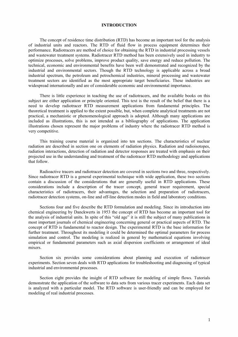
British physicist Ernest Rutherford has discovered three kinds of radiation emitted by so-called

radioactive materials, which he named after the first three letters of the Greek alphabet, alpha (α), beta (β) and gamma (γ). When Rutherford subjected a radioactive material to an electric field, he found out that the radiation was split in three beams (alpha, beta and gamma); alpha and beta were deflected towards opposite electric poles, while gamma not (Fig. 2).

FIG. 2. Alpha, beta and gamma under the effect of magnetic and electrical fields

Alpha particles Alpha decay is a radioactive process in which a particle with two protons and two neutrons is

ejected from the nucleus of a radioactive atom (Fig. 3). The alpha particle is similar to the nucleus of a helium atom. This decay occurs in very heavy elements such as uranium, thorium and radium. The nuclei of these atoms contain more neutrons than protons. Alpha particles have a charge of +2 units

3

due to the two protons and are relatively heavy and energetic compared to other radioactive emissions; this causes alpha particles to interact readily with materials they encounter, including air, causing much ionization in a very short distance. This is referred to as a high linear energy transfer (LET). Most alpha particles have energies between 4 and 6 MeV, will only travel a few centimeters in air and are usually stopped by a sheet of paper.

The observed half-lives are from microseconds to billions of years. This type of radiation poses

an internal health hazard via inhalation, ingestion or absorption through the skin.

FIG. 3. Alpha decay

Beta particles There are two kinds of beta particles: beta minus (electron) and beta plus (positron). These

particles derive from the process of a proton becoming a neutron or vice versa; if a neutron becomes a proton, a negatively charged electron is emitted; when a proton changes to a neutron a positively charged positron is emitted. Because electron and positron are emitted from the nucleus of the atom, they are called beta particle to distinguish them from the electrons that orbit the atom. A neutrino (or anti-neutrino) is also emitted during decay; it is a neutral particle that has almost no mass and carries away some of the energy from the decay process. Figure 4 shows the beta decay of K-40.

FIG. 4. Beta decay

Beta minus (or plus) particles have a single negative (or positive) charge and have a mass only a

small fraction of a neutron or proton. As a result, beta particles interact less readily with material than alpha particles. Depending on the beta particle’s energy (which depends on the radioactive isotope), beta particles may travel up to several meters in air and are stopped by thin layers of metal or plastic. Beta particles are only considered hazardous if they are ingested or inhaled.

After an alpha or beta decay reaction, the nucleus is often left in an "excited" state meaning that

the decay has produced a nucleus that still has excess energy to get rid of. This energy is lost by

4

emitting a pulse of electromagnetic radiation called a gamma ray. The gamma ray is identical in nature to light or microwaves, but of very high energy.

Gamma radiation Gamma rays are electromagnetic radiation emitted by radioactive decay; energies range from

ten thousand to ten million electron volts. Like all forms of electromagnetic radiation, the gamma ray has no mass and no charge. Gamma rays interact with material by colliding with the electrons in the shells of atoms.

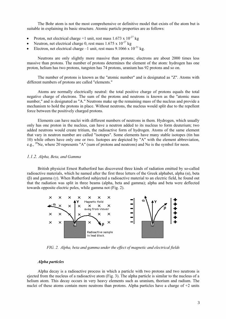
The three interactions are the photoelectric effect, Compton scattering and pair production. They

lose their energy slowly in material, being able to travel significant distances before stopping. Depending on their initial energy, gamma rays can travel up to hundreds of meters in air and can easily penetrate through most of the materials. Most alpha and beta emissions also include gamma rays as part of their decay process. Gamma emission accompanies normally the alpha and beta radiation; there are no "pure" gamma emitters. Gamma radiation poses an external hazard.

Three processes are mainly responsible for the absorption of gamma rays (Fig.5):

• Photoelectric absorption, • Compton scattering, • Pair production (electron-positron).

FIG. 5. Principle of photoelectric absorption, Compton scattering and pair production

For a narrow beam of monoenergetic gamma rays of intensity I0 traveling through a medium of

density ρ, the residual intensity after traversing a thickness x is given by: I = I0exp( - μ.ρ.x)

where: μ is the attenuation coefficient. The above equation strictly applies only to narrow beams of radiation, and this is very difficult

to guarantee in practice. For broad beams of radiation, the equation takes the form:

I = B I0 exp(- μpx) where: B = "build-up" factor. This factor takes a practical detail into account namely the

tendency of gamma rays to be scattered through any medium. Penetration of matter Though the most massive and most energetic of radioactive emissions, alpha particle is the

shortest in range because of its strong interaction with matter. Gamma ray is extremely penetrating, and beta particles strongly interact with matter and have a rather short range (Fig. 6).

5

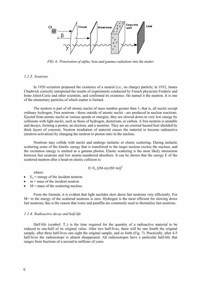
FIG. 6. Penetration of alpha, beta and gamma radiations into the matter

1.1.3. Neutrons

In 1920 scientists proposed the existence of a neutral (i.e., no charge) particle; in 1932, James

Chadwick correctly interpreted the results of experiments conducted by French physicists Frederic and Irene Joliot-Curie and other scientists, and confirmed its existence. He named it the neutron. It is one of the elementary particles of which matter is formed.

The neutron is part of all atomic nuclei of mass number greater than 1; that is, all nuclei except

ordinary hydrogen. Free neutrons - those outside of atomic nuclei - are produced in nuclear reactions. Ejected from atomic nuclei at various speeds or energies, they are slowed down to very low energy by collisions with light nuclei, such as those of hydrogen, deuterium, or carbon. A free neutron is unstable and decays, forming a proton, an electron, and a neutrino. They are an external hazard best shielded by thick layers of concrete. Neutron irradiation of material causes the material to become radioactive (neutron activation) by changing the neutron to proton ratio in the nucleus.

Neutrons may collide with nuclei and undergo inelastic or elastic scattering. During inelastic

scattering some of the kinetic energy that is transferred to the target nucleus excites the nucleus, and the excitation energy is emitted as a gamma photon. Elastic scattering is the most likely interaction between fast neutrons and low atomic-numbered absorbers. It can be shown that the energy E of the scattered neutron after a head-on elastic collision is:

E=Eo [(M-m)/(M+m)]2

where: • Eo = energy of the incident neutron • m = mass of the incident neutron • M = mass of the scattering nucleus

From the formula, it is evident that light nuclides slow dawn fast neutrons very efficiently. For

M= m the energy of the scattered neutrons is zero. Hydrogen is the most efficient for slowing down fast neutrons; this is the reason that water and paraffin are commonly used to thermalize fast neutrons.

1.1.4. Radioactive decay and half-life

Half-life (symbol: T½) is the time required for the quantity of a radioactive material to be

reduced to one-half of its original value. After two half-lives, there will be one fourth the original sample, after three half-lives one eight the original sample, and so forth (Fig. 7). Practically, after 4-5 half-lives the radioisotope is almost disappeared. All radioisotopes have a particular half-life that ranges from fractions of a second to millions of years.

6

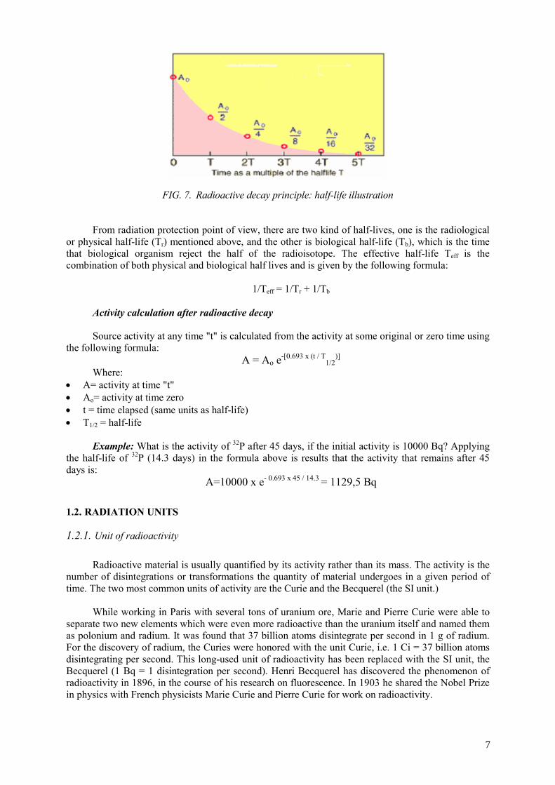
FIG. 7. Radioactive decay principle: half-life illustration

From radiation protection point of view, there are two kind of half-lives, one is the radiological

or physical half-life (Tr) mentioned above, and the other is biological half-life (Tb), which is the time that biological organism reject the half of the radioisotope. The effective half-life Teff is the combination of both physical and biological half lives and is given by the following formula:

1/Teff = 1/Tr + 1/Tb

Activity calculation after radioactive decay Source activity at any time "t" is calculated from the activity at some original or zero time using

the following formula: A = Ao e-[0.693 x (t / T

1/2)]

Where: • A= activity at time "t" • Ao= activity at time zero • t = time elapsed (same units as half-life) • T1/2 = half-life

Example: What is the activity of 32P after 45 days, if the initial activity is 10000 Bq? Applying

the half-life of 32P (14.3 days) in the formula above is results that the activity that remains after 45 days is:

A=10000 x e- 0.693 x 45 / 14.3 = 1129,5 Bq

1.2. RADIATION UNITS

1.2.1. Unit of radioactivity

Radioactive material is usually quantified by its activity rather than its mass. The activity is the

number of disintegrations or transformations the quantity of material undergoes in a given period of time. The two most common units of activity are the Curie and the Becquerel (the SI unit.)

While working in Paris with several tons of uranium ore, Marie and Pierre Curie were able to

separate two new elements which were even more radioactive than the uranium itself and named them as polonium and radium. It was found that 37 billion atoms disintegrate per second in 1 g of radium. For the discovery of radium, the Curies were honored with the unit Curie, i.e. 1 Ci = 37 billion atoms disintegrating per second. This long-used unit of radioactivity has been replaced with the SI unit, the Becquerel (1 Bq = 1 disintegration per second). Henri Becquerel has discovered the phenomenon of radioactivity in 1896, in the course of his research on fluorescence. In 1903 he shared the Nobel Prize in physics with French physicists Marie Curie and Pierre Curie for work on radioactivity.

7

1 Ci = 3,7 x 1010 Bq The Curie is a large amount of radioactivity while the Becquerel is a very small amount. For

convenience, milli- (1 thousandth) and micro- (1 millionth) Curies or Mega- (million) and Giga (billion) Becquerel’s are used in everyday practice.

1.2.2. Dose units

Dose is a generic term that means absorbed dose, dose equivalent, effective dose equivalent,

committed dose equivalent or total effective dose equivalent. Each of these is defined below: Absorbed dose: It is the energy imparted by ionizing radiation per unit mass of irradiated

material, and its measurement unit is the Gray (Gy). Gray is defined as a unit of energy absorbed from ionizing radiation, equal to 10 000 ergs per gram or 1 joule per kilogram of irradiated material. The unit Gray can be used for any type of radiation; it does not describe the biological effects of the different radiations. The old unit of absorbed dose is “rad”. New and old units are relation is: 1 Gray (Gy) = 100 rads.

Equivalent dose: This relates the absorbed dose in human tissue to the effective biological

damage of the radiation. It is a multiplication of (absorbed dose) x (quality factor) x (other necessary modifying factors of interest). The Sievert (Sv) is a unit used to derive the "equivalent dose". Normally, the equivalent dose is expressed in milliSieverts (mSv).

Not all radiations have the same biological effect, even for the same amount of absorbed dose.

Equivalent dose is calculated by multiplying absorbed dose (Gy) by a quality factor (QF) that is unique to the type of incident radiation. Quality factors (QF) for some radiations are: • Gamma and X rays: 1 • Beta particles: 1 • Alpha particles: 20 • Thermal neutrons (lower energy): 2 • Fast neutrons (higher energy): 10 • Protons: 10 • Heavy ions: 20

Roentgen (R): The roentgen is a unit used to measure a quantity called "exposure". This unit is

used only for gamma and X rays with energy less then 3.5 MeV, and only applies in air. One roentgen is equivalent to depositing 2.58 x 10-4 coulombs per kg of dry air. It is a measure of the ionizations of molecules in a mass of air. The main advantage of the Roentgen is that it is easily measured directly.

1.2.3. Radiation dose rate in the vicinity of a point source of gamma rays

There is an empirical relation between the radiation dose rate in air (exposure in R/h) and the

activity A (Ci) of a point source of gamma rays in a distance r (m):

P = Γ . A/r2 where: dose rate factor Γ is an empirical factor for the specific radioisotope that includes

absorption, geometry, photon per disintegration, energy, and all other factors that affect the dose rate from the radioisotope at unit distance. The inverse-square law of gamma absorption in air is assumed as long as the source can be considered a point source. The absorption of gamma rays in air is also assumed to be negligible. Dose rate factors are given in R/h for 1 Ci at 1 m. Γ factors are usually tabulated for activity of 1 Ci and distance of 1 meter. For example 60Co has the dose rate factor of

8

1.35, 137Cs of 0.30, and 198Au of 0.23. This empirical relation is used in field radiotracer work as a simple approach for rough calibration of radiation detectors.

1.3. RADIATION DETECTION

Since radiation cannot be detected with normal senses, special instruments are designed to

indicate the presence of ionizing radiations. The phosphorescent screen where Roentgen observed X ray was the first real-time detector and the precursor to the scintillation crystal detectors still in use today.

The gas filled radiation detector was discovered by Hans Geiger while working with Ernest

Rutherford in 1908. The design of this device was later refined by Hans Geiger and W. Mueller, in the 1920s. It is sometimes called simply a Geiger counter or a G-M counter and is commonly used in portable radiation detection instruments.

The function of a radiation detector is to convert radiation energy into an electrical signal. There

are two basic mechanisms for converting this energy: excitation and ionization. In ionization, an electron is stripped from an atom, and electron and resulting ion are electrically charged. These charged particles can be influenced by an electric field to induce a current that can be measured directly or converted into a voltage pulse. Ionization chambers, Geiger Mueller tubes, BF3 or 3He neutron detectors, and other gas proportional detectors are examples of ionization detectors.

In excitation, electrons are excited to a higher energy level and when the vacant electron is

filled, electromagnetic radiation is emitted. Scintillation detectors such as NaI, BGO, CsI, Polyvinyl toluene (PVT) plastic scintillator and neutron sensitive glass fibers are examples of scintillation detectors. Scintillation crystals respond to radiation by emitting a flash of light proportional to the energy of the photon that is stopped in the crystal. Photomultiplier tubes are used to convert the light emitted by these detectors into electrical pulses which can then be processed.

The most recent class of detector developed are semiconductor (or solid state) detectors. These

detectors convert the incident photons directly into electrical pulses. Solid state detectors are fabricated from a variety of materials including: germanium, silicon, cadmium telluride, mercuric iodide, and cadmium zinc telluride. Choice of detector for a given application depends on several factors. For instance, germanium detectors have the best resolution, but require liquid nitrogen cooling which makes them impractical for portable applications. Silicon, on the other hand, needs no cooling, but is inefficient in detecting photons with energies greater than a few tens of keV. In the last few years detectors fabricated from high Z semiconductor materials have gained acceptance due to their ability to operate at room temperature and their inherent high efficiency. Detectors made from cadmium telluride and cadmium zinc telluride are routinely used.

1.3.1. Gas filled radiation detectors

The most common type of instrument is a gas filled radiation detector. Ionization chamber, gas

proportional and Geiger Muller detectors for alpha, beta and gamma rays, as well as BF3 and He-3 gas proportional detectors for neutrons are examples of gas filled detectors. These detectors work on the principle that as radiation passes through air or a specific gas, ionization of the molecules in the air occurs (Fig.8).

9

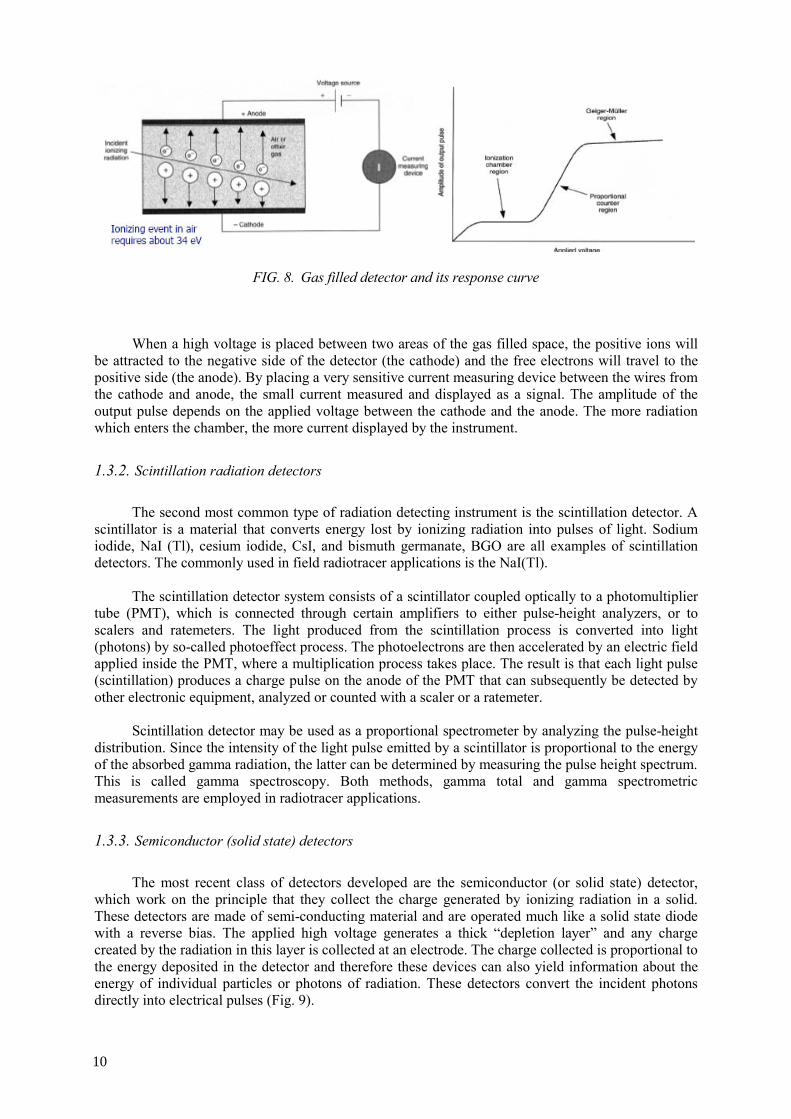
FIG. 8. Gas filled detector and its response curve

When a high voltage is placed between two areas of the gas filled space, the positive ions will

be attracted to the negative side of the detector (the cathode) and the free electrons will travel to the positive side (the anode). By placing a very sensitive current measuring device between the wires from the cathode and anode, the small current measured and displayed as a signal. The amplitude of the output pulse depends on the applied voltage between the cathode and the anode. The more radiation which enters the chamber, the more current displayed by the instrument.

1.3.2. Scintillation radiation detectors

The second most common type of radiation detecting instrument is the scintillation detector. A

scintillator is a material that converts energy lost by ionizing radiation into pulses of light. Sodium iodide, NaI (Tl), cesium iodide, CsI, and bismuth germanate, BGO are all examples of scintillation detectors. The commonly used in field radiotracer applications is the NaI(Tl).

The scintillation detector system consists of a scintillator coupled optically to a photomultiplier

tube (PMT), which is connected through certain amplifiers to either pulse-height analyzers, or to scalers and ratemeters. The light produced from the scintillation process is converted into light (photons) by so-called photoeffect process. The photoelectrons are then accelerated by an electric field applied inside the PMT, where a multiplication process takes place. The result is that each light pulse (scintillation) produces a charge pulse on the anode of the PMT that can subsequently be detected by other electronic equipment, analyzed or counted with a scaler or a ratemeter.

Scintillation detector may be used as a proportional spectrometer by analyzing the pulse-height

distribution. Since the intensity of the light pulse emitted by a scintillator is proportional to the energy of the absorbed gamma radiation, the latter can be determined by measuring the pulse height spectrum. This is called gamma spectroscopy. Both methods, gamma total and gamma spectrometric measurements are employed in radiotracer applications.

1.3.3. Semiconductor (solid state) detectors

The most recent class of detectors developed are the semiconductor (or solid state) detector,

which work on the principle that they collect the charge generated by ionizing radiation in a solid. These detectors are made of semi-conducting material and are operated much like a solid state diode with a reverse bias. The applied high voltage generates a thick “depletion layer” and any charge created by the radiation in this layer is collected at an electrode. The charge collected is proportional to the energy deposited in the detector and therefore these devices can also yield information about the energy of individual particles or photons of radiation. These detectors convert the incident photons directly into electrical pulses (Fig. 9).

10

FIG. 9. Principle of semiconductor (solid state) detector

Solid state detectors are fabricated from a variety of materials including: germanium, silicon,

cadmium telluride, mercuric iodide, and cadmium zinc telluride. The best detector for a given application depends on several factors. For instance, germanium detectors have the best resolution, but require liquid nitrogen cooling which makes them impractical for portable applications. Silicon, on the other hand, needs no cooling, but is inefficient in detecting photons with energies greater than a few tens of keV (kilo electron volts). In the last few years detectors fabricated from high Z semiconductor materials have gained acceptance due to their ability to operate at room temperature and their inherent high efficiency. Detectors made from cadmium telluride, mercuric iodide, and cadmium zinc telluride are routinely used.

1.3.4. Detector efficiency

More than any other part of the detection system the detector itself determines the overall

response function and therefore the sensitivity and minimum detectable count rate of the system. For any detector, there are two important parameters that affect the overall efficiency of the system, geometric efficiency and intrinsic efficiency. By multiplying these values, one can calculate the total efficiency:

• Total efficiency = Geometric efficiency x Intrinsic efficiency • Counts/Emitted radiations = (Incident /Emitted) x (Counts/Incident) radiations

In radiation measurements, the geometric efficiency is the ratio of the number of radiation

particles or photons that hit the detector divided by the total number of radiation particles or photons emitted from the source in all directions. Geometric efficiency is the solid angle subtended by the detector’s active area divided by the area of a sphere whose radius is the distance from the radiation source to the detector. For example, if 10000 gamma rays are emitted from a source and 100 hit the detector then the geometric efficiency εg is 1%.

The geometric efficiency follows a 1/r2 relationship and it drops rapidly as distance increases.

For every doubling of the distance, the geometric efficiency decreases by a factor of 4. For example, for a NaI(Tl) 3"x3" detector, the geometric efficiency of 1% would be reached at about 20 cm from the source.

The intrinsic efficiency is the ratio of counts detected to the number of photons or particles

incident on the detector and is a measure of how many photons or particles result in a gross count. The intrinsic efficiency of various detectors may range from 100% to very small values such as 0.01%, but are typically around 10 to 50%.

11

The product of these two efficiencies is the total efficiency, or the number of counts detected, relative to the total number of radiations emitted from the source. As a result, the actual count measured by the system is a fraction of the radiation emitted in the direction of the detector.

Efficiency of radiation detection is expressed in counts per second per specific activity unit

(counts x s-1 x Bq-1 x m3, or: cps/μCi/m3). Scintillation detectors NaI(Tl) are commonly used for industrial tracer applications because of their high efficiency for gamma ray detection. The intrinsic efficiency of a 1”x1” NaI(Tl) crystal size detector for 100 keV, 500 keV and 1 MeV energy photon is about 39%, 26%, 10% respectively. For NaI (Tl) 2”x2”, which are commonly used in field tests, the intrinsic efficiency is almost four times higher than for 1”x1”.

1.4. RADIATION PROTECTION AND SAFETY

1.4.1. ALARA principle

Radiotracers emit ionizing radiations, which are potentially hazardous to health and therefore

radiation protection measures are necessary throughout all stages of operations. The dose rate at a point is inversely proportional to the square of the distance between the source and the point. Therefore a radiation worker has to maintain maximum possible distance from a radiation source. The dose received is directly proportional to the time spent in handling the source. Thus the time of handling should be as short as possible.

The radiation intensity at a point varies exponentially with the thickness of shielding material.

Thus a radiation worker has to use an optimum thickness of shielding material against the radiating source. The most elementary means of protection is known as "TDS" or "Time, Distance and Shielding."

• Decreasing the time spent around a radiation source decreases the exposure • Increasing the distance from a source decreases the exposure • Increasing the thickness of shielding to absorb or reflect the radiation decreases the exposure

For exposures from any source, except for therapeutic medical exposure, the doses, the number

of people exposed and the likelihood of incurring exposures shall all be kept as low as reasonably achievable (ALARA principle).

1.4.2. Radiation safety considerations in radiotracer applications

All safety measures must be taken to avoid unnecessary exposure to radiation. The following

can be used to facilitate planning of an investigation.

• Radioactive tracers can be detected at low concentrations and through relatively thick walls of pipes and vessels.

• Radiation detectors used are highly sensitive, and can detect radioactivity at low concentrations. • Short half-life tracers can be used. • Normally the volume of process flows ensures that radiotracer is diluted to an acceptably safe

concentration level. • Handling of radioactive tracers must not pose a risk, nor there environmental hazards involved. • During transport of radioactivity to the site of investigation, care should be taken that the dose rate

on the container not be higher than 2 mSv/h (200 mR/h). If transported by vehicle the radiation dose rate must not be higher than 15 μSv/h (1.5 mR/h) in the cabin.

• ALARA must always be the slogan when planning a radioactive tracer investigation.

12

The residual radioactive tracer concentration in the end product should be minimal and at an acceptable concentration level, and, if applicable, be permissible concentration in drinking water. Example: Permissible concentration of 140La in drinking water is 2x10-5μCi/ml set by the International Commission on Radiological Protection (ICRP). For 131I is 2 x 10-6 μCi/ml and is considered safe for consumption by the general public by the ICRP.

Before commencing any radioactive tracer investigation, a complete study must be made

wherein the objectives of the investigation are considered. This will allow the investigator to decide upon the methodology as well as the radioactive tracer to use.

The annual dose limit has to be taken into account and no individual should be exposed beyond

the prescribed limit. This dose limit is 1 mSv/year for a member of the public and 20 mSv/year for a radiation worker, according to European regulations. An effective national infrastructure is a fundamental requirement for safety and security of sources. Safety Series No. 120, Radiation Protection and the Safety of Radiation Sources, Principle 10 states that: “the government shall establish a legal framework for the regulation of practices and interventions, with a clear allocation of responsibilities, including those of a Regulatory Authority”.

The preamble to the Basic Safety Standards (BSS) defines the elements of a national

infrastructure to be: legislation and regulations; a regulatory authority empowered to authorize and inspect regulated activities and to enforce the legislation and regulations; sufficient resources and adequate numbers of trained personnel.

The Regulatory Authority must also be independent of the registrants, licensees and the

designers and constructors of the radiation sources used in practices. Hence users of radiotracers, unless the activity is below the exemption level for that radiotracer, should have an authorization from the appropriate regulatory authority.

A useful IAEA publication that should be used in safety assessments for radiation sources is

IAEA-TECDOC-1113, Safety Assessment Plans for Authorization and Inspection of Radiation Sources. This publication provides practice-specific checklists with items to be considered during the safety assessments that will be included in authorization applications and during the inspections by the Regulatory Authority.

Safety assessments should be made for each application of the tracer having an activity above

the exemption level, since circumstances and the application environment will differ. Each application should consider both occupational and public exposures and ensure that all exposures are as low as reasonably achievable. The level of the assessment should be commensurate with the hazard posed by the radiation source. Hence detailed assessments should not be required where the risk is small, as is the case with many radiotracer experiments.

The procedures for monitoring workers, including the type of dosimeter, should be chosen in

consultation with a qualified expert, such as the radiation protection officer, or as specified by the Regulatory Authority. Depending on the situation, both direct reading dosimeters and thermoluminescent dosimeters (TLDs) or film badges may be needed. For non-uniform exposures, it may be necessary to wear additional dosimeters e.g. for the hands or fingers. Dose records should be kept for each application, where possible, and be available to the Regulatory Authority if requested.

2. RADIOACTIVE TRACERS

2.1. TYPES OF TRACERS

A tracer is any substance whose atomic or nuclear, physical, chemical, or biological properties

provide for the identification, observation and following of the behavior of various physical, chemical

13

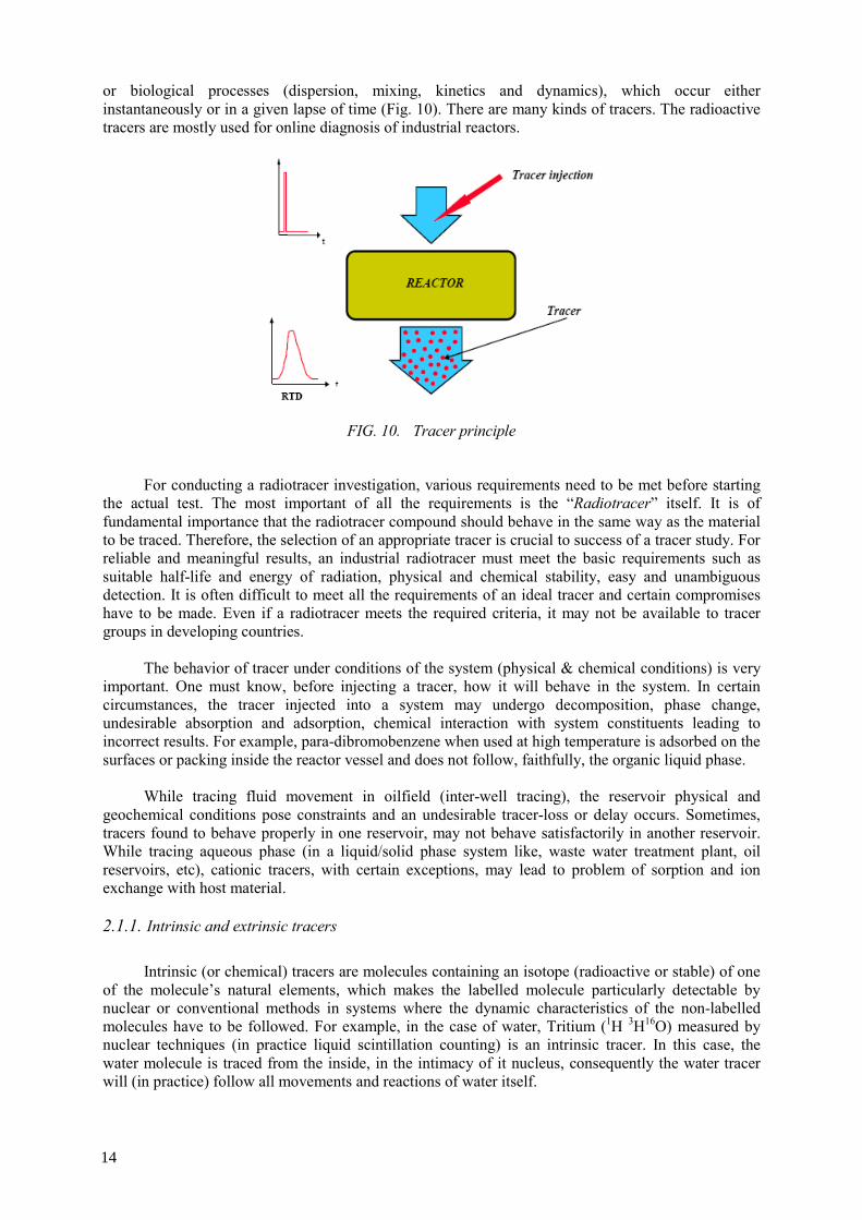
or biological processes (dispersion, mixing, kinetics and dynamics), which occur either instantaneously or in a given lapse of time (Fig. 10). There are many kinds of tracers. The radioactive tracers are mostly used for online diagnosis of industrial reactors.

FIG. 10. Tracer principle

For conducting a radiotracer investigation, various requirements need to be met before starting

the actual test. The most important of all the requirements is the “Radiotracer” itself. It is of fundamental importance that the radiotracer compound should behave in the same way as the material to be traced. Therefore, the selection of an appropriate tracer is crucial to success of a tracer study. For reliable and meaningful results, an industrial radiotracer must meet the basic requirements such as suitable half-life and energy of radiation, physical and chemical stability, easy and unambiguous detection. It is often difficult to meet all the requirements of an ideal tracer and certain compromises have to be made. Even if a radiotracer meets the required criteria, it may not be available to tracer groups in developing countries.

The behavior of tracer under conditions of the system (physical & chemical conditions) is very important. One must know, before injecting a tracer, how it will behave in the system. In certain circumstances, the tracer injected into a system may undergo decomposition, phase change, undesirable absorption and adsorption, chemical interaction with system constituents leading to incorrect results. For example, para-dibromobenzene when used at high temperature is adsorbed on the surfaces or packing inside the reactor vessel and does not follow, faithfully, the organic liquid phase.

While tracing fluid movement in oilfield (inter-well tracing), the reservoir physical and

geochemical conditions pose constraints and an undesirable tracer-loss or delay occurs. Sometimes, tracers found to behave properly in one reservoir, may not behave satisfactorily in another reservoir. While tracing aqueous phase (in a liquid/solid phase system like, waste water treatment plant, oil reservoirs, etc), cationic tracers, with certain exceptions, may lead to problem of sorption and ion exchange with host material.

2.1.1. Intrinsic and extrinsic tracers

Intrinsic (or chemical) tracers are molecules containing an isotope (radioactive or stable) of one

of the molecule’s natural elements, which makes the labelled molecule particularly detectable by nuclear or conventional methods in systems where the dynamic characteristics of the non-labelled molecules have to be followed. For example, in the case of water, Tritium (1H 3H16O) measured by nuclear techniques (in practice liquid scintillation counting) is an intrinsic tracer. In this case, the water molecule is traced from the inside, in the intimacy of it nucleus, consequently the water tracer will (in practice) follow all movements and reactions of water itself.

14

Extrinsic (or physical) tracers are made up of atoms or molecules supposed to share the same dynamic characteristics and, in general, the same mass flow behavior as the investigated medium. Belonging to this category are all the substances that allow tracing outside the molecular or ionic structure. For example, in case of water, Na131I and 51Cr-EDTA are examples of extrinsic tracers for water.

2.2. ADVANTAGES OF RADIOTRACERS

• Most of the radiotracer applications in industrial reactors make use of artificially produced radionuclides. They have high detection sensitivity for extremely small concentrations, for instance, some radionuclides may be detected in quantities as small as 10-17 grams.

• The amount of radiotracer used is virtually insignificant. For example, 1 Ci of 131I- weighs 8 μg, while 1 Ci of 82Br- weighs only 0.9 μg. That’s why, when injected, they do not disturb the dynamics of the system under investigation.

• They offer possibility of “in-situ” measurements, providing information in the shortest possible time.

• A gamma emitting radiotracer can be measured through radiation transmission, from the outside of a pipe or vessel. This is of special importance for many industrial plant studies.

• Disappearance of the radiotracer from the medium under investigation through radioactive decay provides for a repetition of experiments on the same location with the same tracer, all while pollution declines to a minimum.

• Radioactive tracer can be selective. Several tracers may be employed simultaneously and owing to their characteristic radiation emissions, they can be measured accurately with the help of spectrometry.

One of advantages of radiotracer is based on simple fact that it is easier to detect radioactive

than non-radioactive isotopes of the same elements. Vigorous development of analytical technology making possible the attainment of lower and lower detection limits has challenged radioisotope techniques in their most conspicuous stronghold: the limits of detectability.

Advances in the performance of modern instrumental analysis in such branches as gas and

liquid chromatography, fluorimetry, atomic emission, and mass spectrometry are reaching ppb levels. In some applications radiotracers may rank lower (on a comparative basis) than chemical, fluorescent, or stable isotopes regarding some practical aspects. If a non-radioactive tracer can perform the task, it should be preferred. Let’s see some examples.

Example 1: Comparing radiotracer 24Na versus stable isotope 23Na Chemical behavior of radiotracer 24Na is the same of stable 23Na. Detection limits of

conventional analytical techniques for sodium are typically of the order of nanograms, that is (10-9/23) x 6.02 x1023 = 2.6 x1013 atoms. In routine work radiotracer will allow to detect quantities 105 times smaller than conventional techniques.

Example 2: Comparison of tritium measurement techniques Isotope ratio mass spectrometry (IR-MS) detects tritium at the level of 5 TU = 0.59 Bq/L. Low

background liquid scintillation counter (LSC) detects tritium in routine at the level of 1 TU (1 TU equals 1 tritium atom in 1018 hydrogen atoms), so it is clear that LSC is an exceedingly sensitive method.

Example 3: Radiotracer versus rhodamine in water field measurements Let’s compare radiotracer NH4

82Br commonly used in wastewater hydrodynamic investigations, with fluorescent dye Rhodamine-WT, which also is used frequently as water tracer. Rhodamine-WT can be measured down to ppb range in portable fluorometers. Activity concentration of 80 mCi (~3GBq) per g of NH4

82Br is obtained at a low flux reactor at 6.6x1011 n/cm2s. Assuming that 10 g of this irradiated salt suffers a quite high dilution in about 106 m3 of water, resulting mean activity

15

concentration is about 3x104 Bq/m3 = 30 Bq/L, which can be measured very easy. Rhodamine-WT is sold as a 20% solution. Thus, after it suffered same dilution concentration would be 2 ppb. This is only slightly above detection limit of fluorometers, but many times higher than the concentration required for radiotracer. It is thus evident that radiation detection is a much more sensitive method. However, if one looks at mass of dye, it would correspond to 2 mg/m3 x 106 m3 = 2000000 mg = 2 Kg, that means 10 L, which still is a handy volume to manipulate elsewhere in fieldwork. This explains why rhodamine is becoming competitive as water tracers, especially in rivers and other water basins.

2.3. SELECTION OF A RADIOTRACER

Factors that are important in selection of a radiotracer are given as follows:

• Physical/chemical compatibility with the material to be traced • Half-life • Specific activity • Type and energy of radiation emitted • Availability and cost • Method of measurement (sampling or in-situ measurement) • Handling of radioactive materials, radiological protection/regulations.

Under certain circumstances, tracer has to be chemically identical with the traced substance and

then one has to use an intrinsic tracer (also called ‘chemical radiotracer’). This is the case when studying chemical reaction kinetics, solubility, vapour pressures, processes dominated by atomic and molecular diffusion, etc. Radioactive isotopes of the traced elements and labelled molecules are used as intrinsic tracers, for example, 1H3HO for water, 24NaOH for NaOH or 14CO2 for CO2, etc..

Whenever the chemical identity of the tracer with the material it follows is not required, the

tracer has merely to fulfill a limited number of not very stringent physical and physiochemical conditions. This type of tracer is commonly referred to as an extrinsic (or physical) radiotracer. The majority of tracer techniques applied in industry make use of these extrinsic radiotracers. When tracing elements or compounds in systems where no chemical changes occur, the radiotracer does not have to be chemically representative of the element or compound. For example, when water in a plant process is being traced, the only requirement of the tracer is that it behaves as the water behaves under the conditions of the plant process.

Some of the many radiotracers that have been successfully used in this case are 198Au as gold chloride (effective tracer 198AuCl4

-), 24Na as sodium nitrate (effective tracer 24Na+), 131I as sodium iodide (effective tracer 131I-).

16

Table I lists some of the commonly used radiotracers in industry.

TABLE I. COMMONLY USED RADIOTRACER IN INDUSTRY

Isotope Half-life Radiation and Energy (MeV)

Chemical Form Tracing of phase

Tritium (3H) 12.6 y Beta, 0.018(100%) Tritiated water Aqueous Sodium-24 15 h Gamma:

1.37(100%) 2.75(100%)

Sodium carbonate Aqueous

Bromine-82 36 h Gamma: 0.55 (70%) 1.32 (27%)

Ammonium bromide, p-dibrom-benzene, Dibrobiphenyl CH3 Br, C2H5Br

Aqueous Organic Organic Gases

Lanthanum-140 40 h Gamma: 1.16 (95%) 0.92 (10%) 0.82(27%) 2.54 (4%)

Lanthanum chloride, Lanthanum oxide

Aqueous/Solids Solids

Gold-198 2.7 d Gamma: 0.41 (99%) Chloroauric acid Aqueous/Solids Mercury-197 2.7 d Gamma: 0.077(19%) Mercury metal Mercury Iodine-131 8.04 d Gamma:

0.36 (80%) 0.64 (9%)

Potassium or Sodium iodide, Iodobenzene

Aqueous Organic

Chromium-51 28 d Gamma: 0.320 (9.8%) Cr-EDTA, CrCl3 Aqueous Technetium-99m 6 h Gamma: 0.14 (90%) Sodium pertechnetate

(TcO4-)

Aqueous

Scandium-46 84 d Gamma: 0.89(100%) 1.84(100%)

Scandium oxide Scandium chloride ScCl3 (Sc3+)

Solids Aqueous/Solids

Xenon-133 5.27 d Gamma: 0.08 (100%) Xenon Gases Krypton-85 10.6 y Gamma: 0.51(0.7% ) Krypton Gases Krypton-79 35 h Gamma: 0.51 (15%) Krypton Gases Argon-41 110 min Gamma: 1.29(99% ) Argon Gases

2.4. METHODS AND TECHNIQUES FOR LABELLING

2.4.1. Solid materials

A. Internal (mass) labelling A common method for labelling of a solid material is direct activation i.e., to irradiate a portion

of the traced material in a neutron flux and induce the necessary activities. Table II gives examples of widely used tracers labelled by direct activation of solids. Specially produced glasses containing a chemical element that can be activated by (n, γ) reactions, are available to any given size distribution and are used very extensively as sand tracers. 198Au, 51Cr, 192Ir and 46Sc are the radioactive nuclides often induced.

17

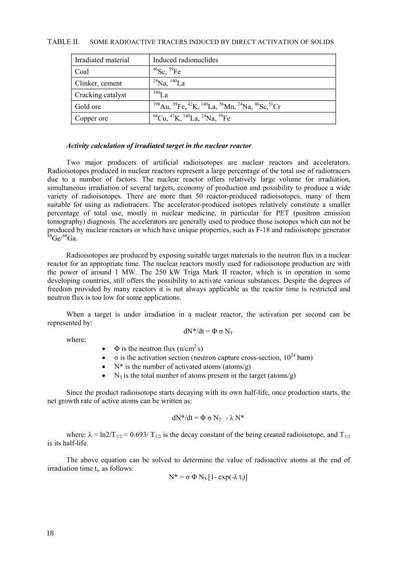
TABLE II. SOME RADIOACTIVE TRACERS INDUCED BY DIRECT ACTIVATION OF SOLIDS

Irradiated material Induced radionuclides Coal 46Sc, 59Fe Clinker, cement 24Na, 140La Cracking catalyst 140La Gold ore 198Au, 59Fe, 42K, 140La, 56Mn, 24Na, 46Sc,51Cr Copper ore 64Cu, 42K, 140La, 24Na, 59Fe

Activity calculation of irradiated target in the nuclear reactor Two major producers of artificial radioisotopes are nuclear reactors and accelerators.

Radioisotopes produced in nuclear reactors represent a large percentage of the total use of radiotracers due to a number of factors. The nuclear reactor offers relatively large volume for irradiation, simultaneous irradiation of several targets, economy of production and possibility to produce a wide variety of radioisotopes. There are more than 50 reactor-produced radioisotopes, many of them suitable for using as radiotracers. The accelerator-produced isotopes relatively constitute a smaller percentage of total use, mostly in nuclear medicine, in particular for PET (positron emission tomography) diagnosis. The accelerators are generally used to produce those isotopes which can not be produced by nuclear reactors or which have unique properties, such as F-18 and radioisotope generator 88Ge/88Ga.

Radioisotopes are produced by exposing suitable target materials to the neutron flux in a nuclear

reactor for an appropriate time. The nuclear reactors mostly used for radioisotope production are with the power of around 1 MW. The 250 kW Triga Mark II reactor, which is in operation in some developing countries, still offers the possibility to activate various substances. Despite the degrees of freedom provided by many reactors it is not always applicable as the reactor time is restricted and neutron flux is too low for some applications.

When a target is under irradiation in a nuclear reactor, the activation per second can be

represented by: dN*/dt = Φ σ NT

where: • Φ is the neutron flux (n/cm2 s) • σ is the activation section (neutron capture cross-section, 1024 barn) • N* is the number of activated atoms (atoms/g) • NT is the total number of atoms present in the target (atoms/g)

Since the product radioisotope starts decaying with its own half-life, once production starts, the

net growth rate of active atoms can be written as:

dN*/dt = Φ σ NT - λ N* where: λ = ln2/T1/2 = 0.693/ T1/2 is the decay constant of the being created radioisotope, and T1/2

is its half-life. The above equation can be solved to determine the value of radioactive atoms at the end of

irradiation time ti, as follows: N* = σ Φ NT [1- exp(-λ ti)]

18

If a delay time (cooling time) td applies after end of irradiation before the radiotracer can be used, the activity A of the irradiated sample at the end of the delay time is:

A = σ Φ NT [1 - exp(-λ ti)] [exp(-λ td )]

Example of sample irradiation and activity calculation Routinely irradiated samples are e.g. KBr-powder to produce 82Br, NaCO3-powder to produce

24Na, argon filled in a 30 ml quartz capsule at a pressure of 10 bars to provide 41Ar, and many others. Let us assume an experiment using 82Br as a radiotracer in the aqueous phase has to be

performed. Normally the target material for production of 82Br is potassium bromide (KBr). What is the needed irradiation time to achieve an amount of activity given a reasonable amount of target material, a relatively standard flux in a nuclear reactor and a desired cooling time for decay of undesired radioisotopes before application?

The production activity is calculated according to the above mentioned formula:

A = σ Φ NT [1- exp(-λ ti)] [exp(–λ td )]

where: σ = the thermal neutron reaction cross section in barn (1 barn=10-24 cm2) φ = the neutron flux (in neutrons/cm2⋅s) NT = the number of target atoms in the target used ti = irradiation time in the nuclear reactor (normally from few minutes to several days) td = cooling time after reactor irradiation (manipulation in the hot cells for preparing the

appropriate radiotracer compound, transport to the experimental site) till injection in the radiotracer test (normally from several hours to few days).

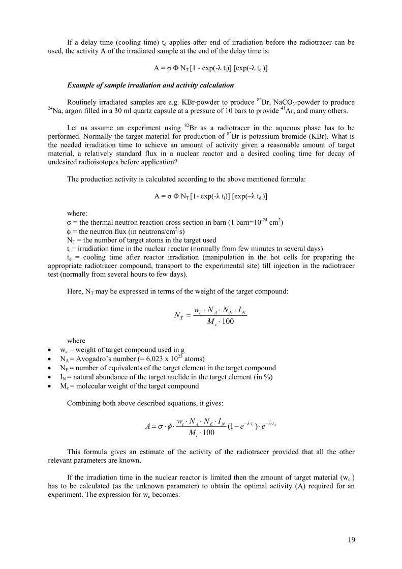
Here, NT may be expressed in terms of the weight of the target compound:

100⋅⋅⋅⋅

=c

NEAcT M

INNwN

where

• wc = weight of target compound used in g • NA = Avogadro’s number (= 6.023 x 1023 atoms) • NE = number of equivalents of the target element in the target compound • IN = natural abundance of the target nuclide in the target element (in %) • Mc = molecular weight of the target compound

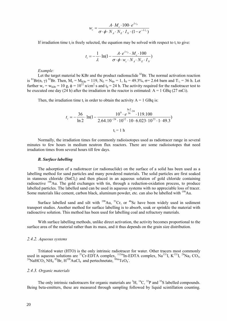
Combining both above described equations, it gives:

di tt

c

NEAc eeM

INNwA ⋅−⋅− ⋅−⋅

⋅⋅⋅⋅⋅= λλφσ )1(

100

This formula gives an estimate of the activity of the radiotracer provided that all the other

relevant parameters are known. If the irradiation time in the nuclear reactor is limited then the amount of target material (wc )

has to be calculated (as the unknown parameter) to obtain the optimal activity (A) required for an experiment. The expression for wc becomes:

19

)1(100

i

d

tNEA

tc

c eINNeMAw ⋅−

⋅

−⋅⋅⋅⋅⋅⋅⋅⋅

= λ

λ

φσ

If irradiation time ti is freely selected, the equation may be solved with respect to ti to give:

)1001ln(1

NEAc

ct

i INNwMeAt

d

⋅⋅⋅⋅⋅⋅⋅⋅

−⋅−=⋅

φσλ

λ

Example: Let the target material be KBr and the product radionuclide 82Br. The normal activation reaction

is 81Br(n, γ) 82Br. Then, Mc = MKBr = 119, NE = NBr = 1, IN = 49.3%, σ= 2.64 barn and T½ = 36 h. Let further wc = wKBr = 10 g, φ = 1012 n/cm2⋅s and td = 24 h. The activity required for the radiotracer test to be executed one day (24 h) after the irradiation in the reactor is estimated: A = 1 GBq (27 mCi).

Then, the irradiation time ti in order to obtain the activity A = 1 GBq is:

)3.49110023.6101010.64.2

100.119101ln(2ln

36231224

2436

2ln9

⋅⋅⋅⋅⋅⋅⋅⋅

−⋅−= −

⋅eti

ti = 1 h

Normally, the irradiation times for commonly radioisotopes used as radiotracer range in several

minutes to few hours in medium neutron flux reactors. There are some radioisotopes that need irradiation times from several hours till few days.

B. Surface labelling The adsorption of a radiotracer (or radionuclide) on the surface of a solid has been used as a

labelling method for sand particles and many powdered materials. The solid particles are first soaked in stannous chloride (SnCl2) and then placed in an aqueous solution of gold chloride containing radioactive 198Au. The gold exchanges with tin, through a reduction-oxidation process, to produce labelled particles. The labelled sand can be used in aqueous systems with no appreciable loss of tracer. Some materials like cement, carbon black, aluminum powder, etc. can also be labelled with 198Au.

Surface labelled sand and silt with 198Au, 51Cr, or 46Sc have been widely used in sediment

transport studies. Another method for surface labelling is to absorb, soak or sprinkle the material with radioactive solution. This method has been used for labelling coal and refractory materials.

With surface labelling methods, unlike direct activation, the activity becomes proportional to the

surface area of the material rather than its mass, and it thus depends on the grain size distribution.

2.4.2. Aqueous systems

Tritiated water (HTO) is the only intrinsic radiotracer for water. Other tracers most commonly

used in aqueous solutions are 51Cr-EDTA complex, 113mIn-EDTA complex, Na131I, K131I, 24Na2 CO3, 24NaHCO3, NH4 82Br, H198AuCl4 and pertechnetate, 99mTcO4

-.

2.4.3. Organic materials

The only intrinsic radiotracers for organic materials are 3H, 14C, 32P and 35S labelled compounds.

Being beta-emitters, these are measured through sampling followed by liquid scintillation counting.

20

Therefore these are rarely used for plant investigations. However they are extensively used in laboratory investigations and in oilfield tracer tests (inter-well tracing).

Extrinsic tracers are more widely used for tracing organic fluids including dibromobiphenyl and

para-dibromobenzene (C6H482Br2), 131I-kerosene and iodobenzene (C6H5

131I), 113mIn in oleate or stearate form. Validation of these tracers in harsh reactor conditions (high temperature and pressure) has to be investigated.

For example, Br-82 as dibromobiphenyl was tested in a trickle bed reactor operating at high

temperature and pressure. The boiling temperature of dibromobiphenyl at atmospheric pressure is 370OC. Since the pressure in the reactor was about 170 kg/cm2, the tracer will not vaporize and will remain in liquid phase at 400 OC. The results of the tracer tests carried out at temperature of 250 0C show that the tracer did not appear at the outlet of the reactor indicating the adsorption of the tracer on the catalyst particles. Another test carried out at lower temperature (~150 0C), showed the tracer did appear at the outlet but the intensity was much less than in the inlet. This indicates partial adsorption of the tracer on catalyst particles. In tracer test carried out at temperature about 100 OC the area under concentration curves recorded were almost equal and the tracer balance was achieved. The results of the tests indicated that at temperature more than 100 0C, the tracer (Br-82 as dibromobiphenyl) gets adsorbed on catalyst particles.

2.4.4. Gaseous materials

Some gas radiotracers can be produced by direct neutron activation in nuclear reactors such as

41Ar and 79Kr. Methyl bromide (CH382Br) is produced through synthesis of radioactive K82Br. Other

commonly used gas radioactive tracer, despite its low energy is 133Xe.

2.5. RADIONUCLIDE GENERATORS FOR INDUSTRIAL APPLICATIONS

2.5.1. Major radionuclide generator-based radiotracers for industrial applications

A radionuclide generator is a chemical/-physical/mechanical devise that is based on mother-

daughter nuclear genetic relationship and allows for the separation and extraction (elution) of the short-lived daughter from the longer-lived stationary mother (Fig.11).

FIG. 11. Principle of radioisotope generator

Several forms of radionuclide generators exist. For the simplest and most common, the parent

radionuclide produced in a nuclear reactor or a cyclotron is adsorbed in a support material such as an ion exchange resin, which is packed in a small column. The short-lived daughter is eluted from the system by using suitable solvents (elutant). After each elution, system is ready for the next elution after about three to four half-lives of the daughter product, during which the daughter product build up will reach near saturation level.

21

The daughter radionuclide extracted from the generator can sometimes be in a chemical form directly suitable as a radiotracer for defined systems. One example is the elution of 99mTc in the form of pertechnetate, 99mTcO4

-, which is a suitable tracer for water flow under certain defined conditions. Most often, the radionuclide extracted needs to be subjected to a labelling procedure to produce the suitable radiotracer. An example of the latter may be the extraction of 113mIn3+ from an 113Sn/113mIn-generator, which needs some form of complexing before use as a water tracer. However, when complexes with ethylenediamine tetra-acetic acid, EDTA, it becomes a suitable water tracer for certain defined conditions.

For a radionuclide generator to be suitable for industrial use, several criteria need to be satisfied.

• Availability: Ideally, the parent radionuclide should be commercially available, at moderate cost. • Half-life of the parent radionuclide: For use at remote locations it is important to select a generator

with an appropriately long half-life. • Half-life of the daughter radionuclide: The daughter radionuclide, used as a radioactive tracer or

tag on the radioactive tracer should have a half-life that is as short as possible, consistent with achieving the objectives of the test. Half-lives varying from several minutes to several hours have been found to be particularly useful. It should also be noted that the shorter the half-life of the daughter, the more rapidly the "cow" regenerates itself after elution of the daughter.

• Type and energy of radiation from the daughter radionuclide: Gamma-ray emitting radionuclides are preferred for most industrial applications because of the ability of gamma radiation to penetrate the often-substantial thicknesses of material from which process plant is constructed. Gamma rays of energy 140 keV and upwards have been found to be useful.

• Physico-chemical properties of the eluted daughter: Ideally, the material eluted from the generator should be in a form that is physically and chemically compatible with the material to be traced so that it can be injected into the process stream of interest without delay and without complicated chemical treatment.

In line with the above criteria, four generators have been found to be particularly suitable for

industrial use. They are briefly described below. 99Mo/99mTc Generator This generator is used extensively in nuclear medicine and is widely available worldwide. For

this reason the somewhat short half-life of the 99Mo is not too severe a disadvantage. The half-life of the daughter 99mTc, i.e. 6 hours, is appropriate for a wide range of studies in industry and environment.

The gamma-ray (140 keV) has a half-thickness of 5 mm of steel. Thus, the 99mTc is suitable as a

tracer for vessels of wall thickness up to about 20 mm. It is not appropriate for use on high-pressure plants. The low gamma-ray energy of 99mTc is sometimes an advantage. The radiotracer, which is usually eluted as sodium pertechnetate solution, has been used to study the detailed fluid dynamics of large-scale water like systems such as wastewater and sewage treatment installations. Detectors submerged in the pond sense only tracer in the immediate vicinity so that localized flow patterns can be observed.

The main advantage of this generator is its availability worldwide from a number of suppliers,

usually at a few days notice and at a cost that is not prohibitive. A 37 GBq generator costs approximately US$2000, which is small in industrial terms. Additionally, from a public relations point of view, prospective clients often perceive a tracer that is used for medical applications as more user-friendly. For all of these reasons, the 99Mo/99mTc generator can be a powerful weapon in the armoury of industrial radiotracer groups and it should not be neglected.

22

137Cs/137mBa Generator 137Cs/137mBa generators are available commercially, but with very low activity (typically 370

kBq), suitable only for use in educational establishments for demonstration purposes. 137Cs/137mBa generator for industrial applications is not commercially available. However, the parent radioisotope, 137Cs, may be purchased from a number of suppliers (137CsCl3) at a reasonable cost, which has led to a number of radiotracer applications groups constructing generators to meet their own particular needs. To provide a generator system it is necessary:

• To attach the cesium chemically onto appropriate support medium. • To provide a suitable system for eluting the 137mBa daughter.

The main drawback to this type of generator is the short half-life (2.55 minutes). Even so, the

generator is suitable for many industrial applications. The typical application of this generator is the flow rate measurement for calibration.

The half-life of the parent isotope at 30 years facilitates long-term storage and the gamma ray

energy of the daughter at 660 keV is high enough for most industrial applications. The potential usefulness of this generator together with a relatively small price tag, warrants its promotion.

113Sn / 113mIn Generator This generator is commercially available, packaged in a lead container that can be eluted readily

using HCl solution injected from a hypodermic syringe. The gamma-ray energy of 390 keV together with the useful half-lives of the 113Sn parent (115 d) and 113mIn daughter (100 min) makes this generator suitable for many industrial applications.

68Ge/68Ga Generator 68Ge/68Ga generator has much to recommend as a source of industrial radiotracer. This is in

many respects similar to the 113Sn/113mIn generator. The parent has a reasonably long half-life (271 days) and the radiations from the daughter (1.08 MeV gamma ray, plus 511 keV annihilation radiation) are sufficiently high to allow its use as a radiotracer on most types of industrial applications, in particular for investigation of processes inside the thick-walled pipes and vessels. The half-life of the 68Ga, at 68 minutes, is relatively short, but sufficiently long for many industrial applications. Commercially available 68Ge/68Ga are currently expensive (approximately US$17000 for 1.85 GBq) and this has acted as a barrier to their acceptance by radioisotope applications groups. The identification of a production route that allows this generator to be offered at a significantly reduced price would be a worthwhile objective for the near future.

2.5.2. Application of radionuclide generator-based radiotracers

Some typical applications of radionuclide generator-based radiotracers can be summarized as

follows: 99mTc in sodium pertechnetate form

• Water tracing in wastewater treatment plants for RTD measurement, injected activity ≈ 4 to18 GBq,

• Water tracing in surface bodies (rivers, sea) for dispersion of effluent studies (outfalls) and dispersion coefficient measurements, injected activity ≈ 37 GBq,

• Water tracing for water infiltration coefficient measurement in soil (K < 10-9 m/s), injected activity ≈ 5 MBq,

• Determination of water channelling in petrol borehole (2000 m depth), injected activity ≈ 6 MBq,

23

• water flow rate measurement in a petrol production borehole (2800 m depth), injected activity ≈ 4 MBq,

• SPECT tomography in an auxiliary circuit of a nuclear power plant to determine mixture efficiency of cold water in hot water, injected activity 300 GBq, 12 injections.

99mTc in reduced SnCl2 medium

• Sludge labelling-tracing in wastewater treatment plants for RTD measurements, injected activity ≈ 4 to 18 GBq,

• Mud labelling-tracing in surface bodies (rivers, sea) for particle dispersion of effluent studies (outfalls) and dispersion coefficient measurements, injected activity ≈ 37 GBq,

• Mud labelling-tracing in sea for dredging products dumping studies (dumping efficiency, advection, dilution, dispersion coefficients, etc…), injected activity ≈ 150 GBq.

99mTc for organic phase tracing (solvent extraction from sodium pertechnetate elutant)

• Lubrification studies on a jet engine prototype, injected activity ≈ 890 MBq, 15 injections, • Leakage detection in a high voltage cable (oil insulation), injected activity ≈ 5 MBq

113mIn in chloride solution

• Sludge labelling-tracing in wastewater treatment plants for RTD measurements, injected activity ≈ 3.7 GBq,

• Mud labelling-tracing for laboratory channel mud dumping studies for CFD model validation, injected activity ≈ 3.7 GBq, 45 injections,

• Catalyst labelling-tracing for RTD and SPECT measurements in a slurry reactor at a pilot plant scale, injected activity ≈ 925 MBq.

113mIn in EDTA complex

• Water tracing in various hydraulic pilot plants and laboratory facilities, injected activity ≈ 0.37 to 3.7 GBq,

• Organic phase tracing for RTD and SPECT measurements in a slurry reactor at a pilot plant scale for IFP, injected activity ≈ 925 MBq.

The table III below summarizes some application cases and conditions.

TABLE III. SOME APPLICATIONS OF RADIONUCLIDE GENERATOR-BASED RADIOTRACERS

Generator Cs-Ba Mo-Tc Sn-In Surface water X X X + EDTA Groundwater X X + EDTA Water WWTP X X X + EDTA Sludge WWTP X + SnCl2 X

Mud in surface water X + SnCl2 X

Organic phase tested < 120 °C

X + TBP X + EDTA

Catalyst in organic phase tested < 120 °C

X

Water high temperature under high pressure

tested < 350°C, 40 bars

X X

24

2.6. MIXING LENGTH ESTIMATION

2.6.1. Definition of mixing length

Mixing length (or good mixing length) is defined as the distance beyond which the variation in

the duct cross-section of tracer concentration C is smaller than some previously chosen value. The mixing length depends among others from the position of injection inside the pipe.

Injection at the centre of the pipe The following equations can be used to estimate mixing length, in terms of length to diameter

L/D ratio (or equivalently in number of pipe diameters), as a function of the admissible variation of the tracer concentration in the cross-section of the pipe, flow Reynolds number Re and wall friction.

( )

⎟⎠⎞

⎜⎝⎛ −

λ=

3.2xln

94.28

18.1DL

(1)

( )

λ−= ⎟

⎠⎞

⎜⎝⎛ 8

4.2xln

95.2DL

(2)

( )( )21

pipe

smooth101

Rexln85.25.20DL

⎟⎟

⎠

⎞

⎜⎜

⎝

⎛

λ

λ−= (3)

where x is the maximum percentage of variation of tracer concentration over the cross-section of the

pipe, λ is the pipe friction coefficient (λsmooth : value for a smooth pipe),

pipeλ is the value for the real pipe. Reynolds number in pipe flow is defined as:

Re = U.D/ν where:

• U is the fluid velocity (m/s), • Ν is the fluid kinematic viscosity (in m2/s), • D is the pipe diameter (m).

Eq. 1 is derived on the assumption of constant radial diffusion coefficient and flat velocity

profile; Eq. 2 on the assumption of parabolic radial diffusion coefficient profile and flat velocity profile; Eq. 3 assumes a parabolic radial diffusion coefficient profile and a logarithmic velocity profile. These equations are plotted in Fig. 12. They show that for Reynolds numbers equal to 105 and a smooth pipe, the “mixing length” (predictably) decreases when x increases.

25

FIG. 12. Mixing length (L/D) versus maximum variation of tracer concentration.

2.6.2. Examples of injection techniques for reducing mixing length

Experience has shown that good cross-sectional mixing may require as many as 100 pipe

diameters to be achieved. It is often not possible to inject the tracer at such a distance upstream of the measurement section. Therefore, it is required to reduce that length by using appropriate tracer injection techniques and devices.

Multiple-orifice injectors Substantial reduction in mixing length can be obtained by injecting the tracer through multiple

orifices uniformly distributed on the pipe wall or (if possible) inside the pipe. High velocity jets Injecting the tracer counter-currently at a velocity much larger than bulk flow velocity induces

high mixing at the end of the jet. The reduction in good mixing length depends on the number and momentum of the jets and on their angle with respect to the main flow direction. A simple jet arrangement can bring about 30% reduction in mixing length as compared to the single central injection point.

Vortex generators Incorporating obstacles within the pipe, just after tracer injection point, produces turbulence that

enhances mixing and reduces mixing length. As an example, injecting the tracer through three triangular plates, at an angle of 40o to the main flow direction, reduces mixing length by one third with respect to a central single injection point.

Pumps and turbines If tracer is injected upstream of a pump or a turbine, mixing length is considerably reduced.

Centrifugal pumps reduce mixing length by about 50 pipe diameters. Bends, valves and other obstacles Every singularity in the pipe promotes turbulence that tends to decrease good mixing length.

However, it is advisable to use straight lengths of pipe without obstacles whenever transit times are to be measured.

Fig.13 shows variation in mixing length for four different types of injection.

26

FIG. 13. Mixing length L/D vs. maximum variation of tracer injection with four types of injection.

Examples of injectors Injection systems are generally home made, built and adapted for specific applications. They

vary considerably in design from the simplest (a syringe or a reservoir with a peristaltic pump) to the most complex (devices for remote injection into pressure vessels). Simple devices for gas and liquid pulse injections are presented in figures 16&17:

FIG. 14. Gas tracer injector.

FIG. 15. Liquid tracer injector

27

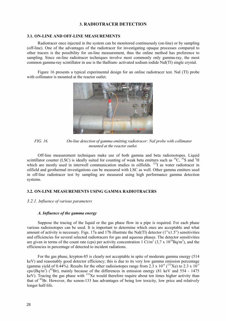
3. RADIOTRACER DETECTION

3.1. ON-LINE AND OFF-LINE MEASUREMENTS

Radiotracer once injected in the system can be monitored continuously (on-line) or by sampling (off-line). One of the advantages of the radiotracer for investigating opaque processes compared to other tracers is the possibility for on-line measurement, thus the online method has preference to sampling. Since on-line radiotracer techniques involve most commonly only gamma-ray, the most common gamma-ray scintillator in use is the thallium- activated sodium iodide NaI(Tl) single crystal.

Figure 16 presents a typical experimental design for an online radiotracer test. NaI (Tl) probe

with collimator is mounted at the reactor outlet.

FIG. 16. On-line detection of gamma emitting radiotracer: NaI probe with collimator mounted at the reactor outlet.

Off-line measurement techniques make use of both gamma and beta radioisotopes. Liquid scintillator counter (LSC) is ideally suited for counting of weak beta emitters such as 14C, 35S and 3H which are mostly used in interwell communication studies in oilfields. 125I as water radiotracer in oilfield and geothermal investigations can be measured with LSC as well. Other gamma emitters used in off-line radiotracer test by sampling are measured using high performance gamma detection systems.

3.2. ON-LINE MEASUREMENTS USING GAMMA RADIOTRACERS

3.2.1. Influence of various parameters

A. Influence of the gamma energy Suppose the tracing of the liquid or the gas phase flow in a pipe is required. For each phase

various radioisotopes can be used. It is important to determine which ones are acceptable and what amount of activity is necessary. Figs. 17a and 17b illustrate the NaI(Tl) detector (1”x1.5”) sensitivities and efficiencies for several selected radiotracers for gas and aqueous phases. The detector sensitivities are given in terms of the count rate (cps) per activity concentration 1 Ci/m3 (3,7 x 1010Bq/m3), and the efficiencies in percentage of detected to incident radiations.

For the gas phase, krypton-85 is clearly not acceptable in spite of moderate gamma energy (514

keV) and reasonably good detector efficiency; this is due to its very low gamma emission percentage (gamma yield of 0.44%). Results for the other radioisotopes range from 2.3 x 10-6 (133Xe) to 2.3 x 10-5 cps/(Bq/m3) (82Br), mainly because of the differences in emission energy (81 keV and 554 - 1475 keV). Tracing the gas phase with 133Xe would therefore require about ten times higher activity than that of 82Br. However, the xenon-133 has advantages of being low toxicity, low price and relatively longer half-life.

28

As regards the liquid phase, 51Cr is handicapped by its low gamma emission percentage (10%). Results for other isotopes are in the 2 10-5 (24Na) to 3.3 10-5 cps/(Bq/m3) (82Br) range, which would result in acceptable values for injected activity. 99mTc, which is commonly used in nuclear medicine diagnosis, despite its low energy is largely used in industrial applications as well.

a) Gas phase

b) Liquid phase

FIG. 17. NaI detector(1”x1.5”) sensitivities and efficiencies for various gas and liquid radiotracers

B. Influence of scintillator crystal nature and dimensions The influence of the nature and the dimensions (diameter and thickness) of the scintillator

crystal on its sensitivity, the count rate (cps) per specific activity 1 Ci/m3 (3,7 x 1010 Bq/m3), and on the efficiency of the detection (%) is shown in figure 18. The radioisotope is 41Ar, scintillator crystal is either 1.5 inch in diameter by 2 inches in thickness or half that size, and either NaI(Tl) or BGO. Not surprisingly with this high energy tracer, efficiency is significantly better with thick crystals and BGO always performs better than NaI(Tl).

29

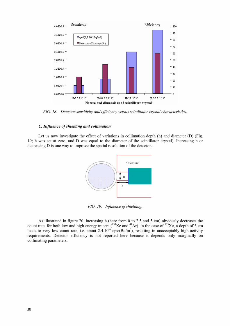
FIG. 18. Detector sensitivity and efficiency versus scintillator crystal characteristics.

C. Influence of shielding and collimation Let us now investigate the effect of variations in collimation depth (h) and diameter (D) (Fig.

19; h was set at zero, and D was equal to the diameter of the scintillator crystal). Increasing h or decreasing D is one way to improve the spatial resolution of the detector.

Shielding

h

D

FIG. 19. Influence of shielding.

As illustrated in figure 20, increasing h (here from 0 to 2.5 and 5 cm) obviously decreases the

count rate, for both low and high energy tracers (133Xe and 41Ar). In the case of 133Xe, a depth of 5 cm leads to very low count rate, i.e. about 2.4.10-6 cps/(Bq/m3), resulting in unacceptably high activity requirements. Detector efficiency is not reported here because it depends only marginally on collimating parameters.

30

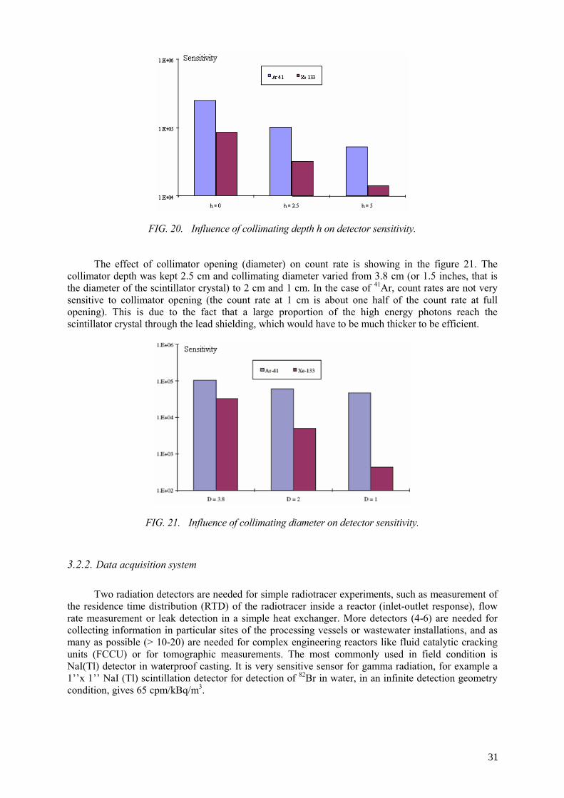
FIG. 20. Influence of collimating depth h on detector sensitivity.

The effect of collimator opening (diameter) on count rate is showing in the figure 21. The

collimator depth was kept 2.5 cm and collimating diameter varied from 3.8 cm (or 1.5 inches, that is the diameter of the scintillator crystal) to 2 cm and 1 cm. In the case of 41Ar, count rates are not very sensitive to collimator opening (the count rate at 1 cm is about one half of the count rate at full opening). This is due to the fact that a large proportion of the high energy photons reach the scintillator crystal through the lead shielding, which would have to be much thicker to be efficient.

FIG. 21. Influence of collimating diameter on detector sensitivity.

3.2.2. Data acquisition system

Two radiation detectors are needed for simple radiotracer experiments, such as measurement of

the residence time distribution (RTD) of the radiotracer inside a reactor (inlet-outlet response), flow rate measurement or leak detection in a simple heat exchanger. More detectors (4-6) are needed for collecting information in particular sites of the processing vessels or wastewater installations, and as many as possible (> 10-20) are needed for complex engineering reactors like fluid catalytic cracking units (FCCU) or for tomographic measurements. The most commonly used in field condition is NaI(Tl) detector in waterproof casting. It is very sensitive sensor for gamma radiation, for example a 1’’x 1’’ NaI (Tl) scintillation detector for detection of 82Br in water, in an infinite detection geometry condition, gives 65 cpm/kBq/m3.

31

Detection probes are mounted at selected locations at the inlet and outlet of the processing vessel and are shielded by lead collimators to protect them from the natural background and other parasite radiation may come from around. If needed, detectors are protected from heat (for temperature higher than 60-700C) by placing aluminum plate between the detector and reactor walls.

The data acquisition system, which collects signals from the radiation detectors, is the basic

equipment for online radiotracer work. The data acquisition system ensures collection, treatment and visualization of the data. Dead time between two measurements is normally less than 1 µs. The visualization of data is as close as possible to “real time” experiment. The measurements are simultaneous and the minimal dwelling time is 1-2 ms. Standard portable data acquisition systems for industrial radiotracer work are PC based data logger with unlimited possibility in the number of connected probes. There are several prototypes of data acquisition system (commercial or homemade). Figure 22 shows some of them:

FIG. 22. Data acquisition systems for online radiotracer tests

The data acquisition software consists of three main different functions:

• Controlling the operational functioning of probes, • Data processing during the tracing experiment. For each probe it should be possible to set several

(for example 5) measuring intervals. Each measuring interval is defined by its duration, and by the counting time ranging between 1 ms and 1 hour (h). It should be emphasized that the measurements have to be simultaneous for all active channels. The software has to ensure acquisition, basic treatment and visualization of the data. Dead time between two measurements should be less than 1 µs. The visualization of data should be as close as possible to “real time” refreshment of the graphical window.

• Allowing the user to read and display acquired data.

32

3.3. OFF-LINE MEASUREMENTS

3.3.1. Sampling measurement

Measuring techniques for samples depend on which kind of radiotracers (beta or gamma) is

used. When counting a radioactive sample it is well known that instrument reading is a measure of sample activity plus background. The latter must be subtracted in order to evaluate the net sample activity. Background is usually measured by using samples taken before the injection (blank sample).

A. Beta-radioactive tracers The most common beta-radioactive tracers for interwell studies are labelled with tritium (3H),

carbon-14 (14C) or sulphur-35 (35S). All of them are usually measured by means of liquid scintillation counting (LSC) technique. A small volume of a liquid sample is mixed with a special solution known as scintillation cocktail, commonly in a 20 mL light transparent (glass, polypropylene, teflon) vial. Beta particles cause emission of light when passing through and slowing down in the scintillation cocktail. These light pulses are registered by photo-multiplier (PMT) suitable for that particular photon wavelength. The light intensity is proportional to the energy of the beta particle. This process is called scintillation, and since it happens in liquid media, it is known as liquid scintillation. The vial is placed inside the LSC, and two PMTs operate in co-incidence mode to reduce background. The LSC analyses the pulses from the PMTs and provides information about the energy of the beta particles and the rate of beta emission (activity) in the sample.

Various processes may perturb the beta-spectrum obtained in a liquid scintillation process. The

most important are chemical and physical quenching. Chemical and physical quenching: Some components or particles in the sample may prevent light

from being detected by the PMTs. Some chemicals may absorb the energy and release it in the form of heat. Heavy chemical quenchers are for instance organic compounds containing oxygen and in particular chlorine. All these forms of quenching result in a shift of the energy spectrum towards lower channels and the number of photons detected by the PMTs per beta decay is reduced. Quenching may change from one sample to another. Evaluation of quenching effect is necessary in order to calculate counting efficiency.

As a conclusion: Liquid scintillation counting requires careful sample preparation. Most often,

chemical separations are involved. When these procedures are optimized, very low detection limits may be obtained ranging from 2 Bq/L for HTO to <0.02 Bq/L for S14CN- .

B. Gamma radioactive tracers Gamma tracers are commonly measured using either solid scintillation or semiconductor detectors. Solid scintillation detectors: These are of different types, but the most generally applicable is the

detector based on a single crystal of sodium iodide doped with traces of thallium, the so-called NaI (Tl)-detector. The crystal is optically coupled to a photomultiplier (PMT). Interaction of a gamma photon with the scintillation crystal results in emission of light, which is detected by the PMT. The light output is proportional to the gamma energy. The electronic system associated to the PMT analyses the pulses according to pulse amplitude (energy) and stores the results in a multichannel analyzer (MCA). Thus, energy and intensity are recorded, and the result is the gamma energy spectrum of the radiation source. NaI(Tl)-detector has a high intrinsic efficiency but a limited energy resolution. They are available in different sizes. Commonly used crystals are of sizes of 2” x 2” - 3” x 3” (height x diameter). The NaI(Tl) detectors can be made quite rugged, and are suitable for field instrumentation.

33

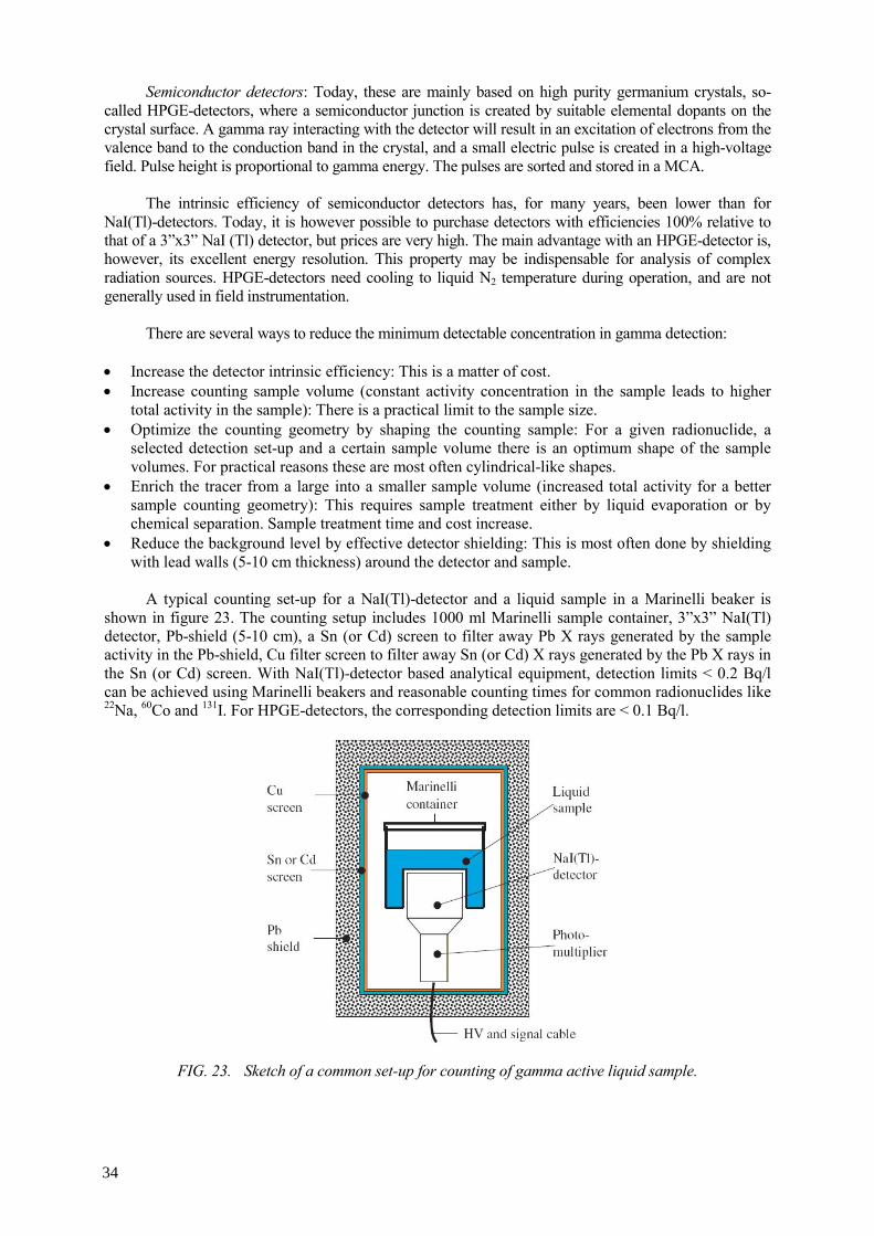
Semiconductor detectors: Today, these are mainly based on high purity germanium crystals, so-called HPGE-detectors, where a semiconductor junction is created by suitable elemental dopants on the crystal surface. A gamma ray interacting with the detector will result in an excitation of electrons from the valence band to the conduction band in the crystal, and a small electric pulse is created in a high-voltage field. Pulse height is proportional to gamma energy. The pulses are sorted and stored in a MCA.

The intrinsic efficiency of semiconductor detectors has, for many years, been lower than for

NaI(Tl)-detectors. Today, it is however possible to purchase detectors with efficiencies 100% relative to that of a 3”x3” NaI (Tl) detector, but prices are very high. The main advantage with an HPGE-detector is, however, its excellent energy resolution. This property may be indispensable for analysis of complex radiation sources. HPGE-detectors need cooling to liquid N2 temperature during operation, and are not generally used in field instrumentation.

There are several ways to reduce the minimum detectable concentration in gamma detection:

• Increase the detector intrinsic efficiency: This is a matter of cost. • Increase counting sample volume (constant activity concentration in the sample leads to higher

total activity in the sample): There is a practical limit to the sample size. • Optimize the counting geometry by shaping the counting sample: For a given radionuclide, a

selected detection set-up and a certain sample volume there is an optimum shape of the sample volumes. For practical reasons these are most often cylindrical-like shapes.

• Enrich the tracer from a large into a smaller sample volume (increased total activity for a better sample counting geometry): This requires sample treatment either by liquid evaporation or by chemical separation. Sample treatment time and cost increase.

• Reduce the background level by effective detector shielding: This is most often done by shielding with lead walls (5-10 cm thickness) around the detector and sample.

A typical counting set-up for a NaI(Tl)-detector and a liquid sample in a Marinelli beaker is

shown in figure 23. The counting setup includes 1000 ml Marinelli sample container, 3”x3” NaI(Tl) detector, Pb-shield (5-10 cm), a Sn (or Cd) screen to filter away Pb X rays generated by the sample activity in the Pb-shield, Cu filter screen to filter away Sn (or Cd) X rays generated by the Pb X rays in the Sn (or Cd) screen. With NaI(Tl)-detector based analytical equipment, detection limits < 0.2 Bq/l can be achieved using Marinelli beakers and reasonable counting times for common radionuclides like 22Na, 60Co and 131I. For HPGE-detectors, the corresponding detection limits are < 0.1 Bq/l.

FIG. 23. Sketch of a common set-up for counting of gamma active liquid sample.

34

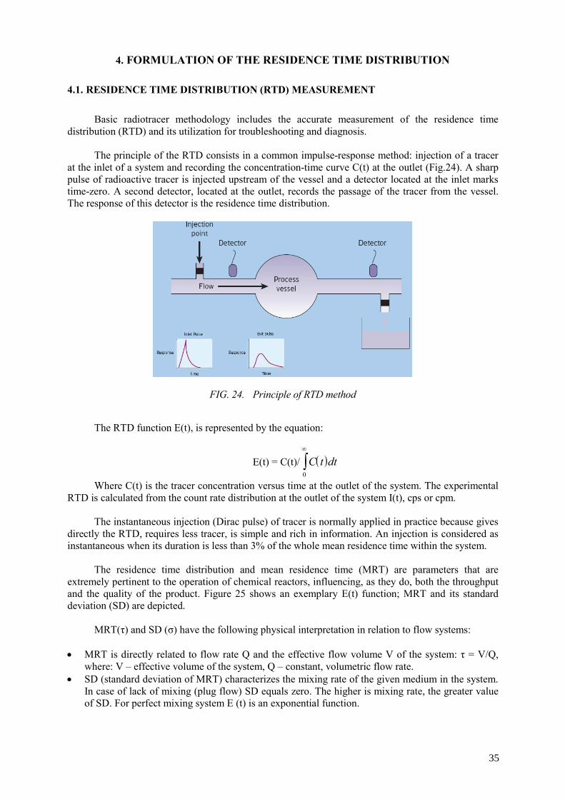
4. FORMULATION OF THE RESIDENCE TIME DISTRIBUTION

4.1. RESIDENCE TIME DISTRIBUTION (RTD) MEASUREMENT

Basic radiotracer methodology includes the accurate measurement of the residence time

distribution (RTD) and its utilization for troubleshooting and diagnosis. The principle of the RTD consists in a common impulse-response method: injection of a tracer

at the inlet of a system and recording the concentration-time curve C(t) at the outlet (Fig.24). A sharp pulse of radioactive tracer is injected upstream of the vessel and a detector located at the inlet marks time-zero. A second detector, located at the outlet, records the passage of the tracer from the vessel. The response of this detector is the residence time distribution.

FIG. 24. Principle of RTD method

The RTD function E(t), is represented by the equation:

E(t) = C(t)/ ( )C t dt0

∞

∫

Where C(t) is the tracer concentration versus time at the outlet of the system. The experimental RTD is calculated from the count rate distribution at the outlet of the system I(t), cps or cpm.

The instantaneous injection (Dirac pulse) of tracer is normally applied in practice because gives

directly the RTD, requires less tracer, is simple and rich in information. An injection is considered as instantaneous when its duration is less than 3% of the whole mean residence time within the system.

The residence time distribution and mean residence time (MRT) are parameters that are

extremely pertinent to the operation of chemical reactors, influencing, as they do, both the throughput and the quality of the product. Figure 25 shows an exemplary E(t) function; MRT and its standard deviation (SD) are depicted.

MRT(τ) and SD (σ) have the following physical interpretation in relation to flow systems:

• MRT is directly related to flow rate Q and the effective flow volume V of the system: τ = V/Q, where: V – effective volume of the system, Q – constant, volumetric flow rate.

• SD (standard deviation of MRT) characterizes the mixing rate of the given medium in the system. In case of lack of mixing (plug flow) SD equals zero. The higher is mixing rate, the greater value of SD. For perfect mixing system E (t) is an exponential function.

35

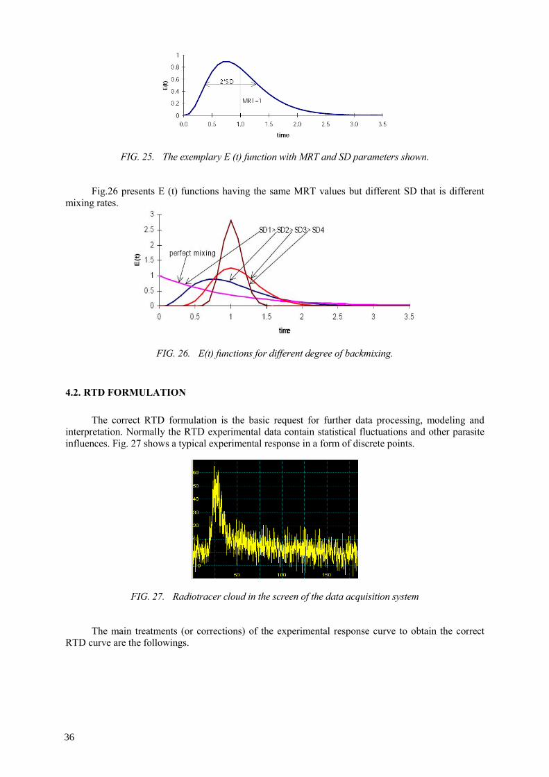
FIG. 25. The exemplary E (t) function with MRT and SD parameters shown.

Fig.26 presents E (t) functions having the same MRT values but different SD that is different

mixing rates.

FIG. 26. E(t) functions for different degree of backmixing.

4.2. RTD FORMULATION The correct RTD formulation is the basic request for further data processing, modeling and

interpretation. Normally the RTD experimental data contain statistical fluctuations and other parasite influences. Fig. 27 shows a typical experimental response in a form of discrete points.

FIG. 27. Radiotracer cloud in the screen of the data acquisition system

The main treatments (or corrections) of the experimental response curve to obtain the correct

RTD curve are the followings.

36

4.2.1. Dead time correction

Nearly all detector systems have a minimum amount of time that must separate two gamma photons in order that they are recorded as two separate pulses. This minimum time delay (or dead time, τ) may be due either to the physical detection process itself or to associated electronic devices.

The relation between the true nt(t) and the measured nm(t)count rate is as follows:

With a dead time of 10 μs the error is less than 10% up to the fairly high value of 104 cps.

4.2.2. Background correction

Prior to the injection of radiotracer into a system, it is necessary to measure the background radiation level, which is subtracted from the experimental data (Fig. 28).

FIG. 28. Raw signal and background corrected signal

4.2.3. Radioactive decay correction

Since radioisotope tracers decay exponentially with time, it is necessary to apply decay correction to the measured data (otherwise, more weight would unduly be given to early measurements). The decay corrected count rate nc(t) is given as:

Where: λ is the decay constant, t is the time and T½ is the half-life of the radioisotope tracer. The effect of the correction for the radioactive decay in radiotracer applications is illustrated in

the figure 29. The blue experimental curve in the figure 29 presents the results of the radioisotope tracing with 113mIn (half-life 5970 s). Because of the relatively long duration of experimental measurement (1400 s) the radioactive decay correction is necessary. The real experimental curve corrected for radioactive decay of 113mIn is shown in the same figure 29 in red color. If the decay correction is not applied, one gets the wrong impression that the tracer concentration is decreasing at the end of experiment (blue curve uncorrected). Applying the decay correction shows that the tracer concentration actually has reached a constant level (red curve corrected).

37

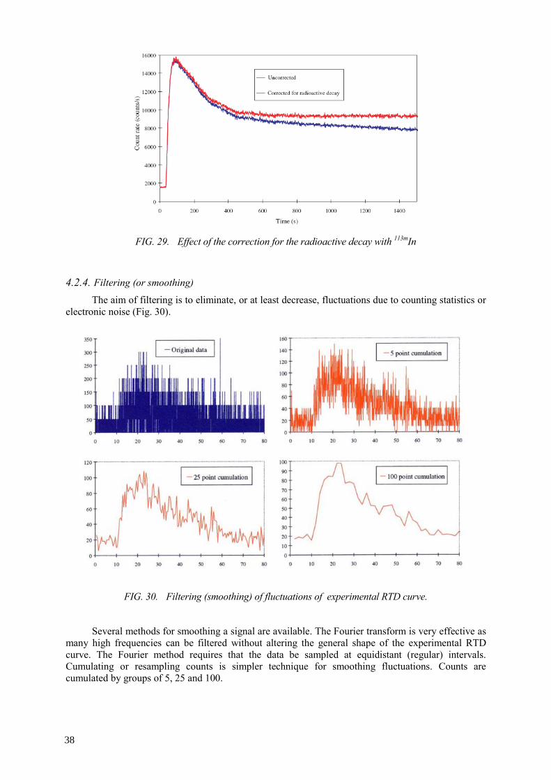
FIG. 29. Effect of the correction for the radioactive decay with 113mIn

4.2.4. Filtering (or smoothing)

The aim of filtering is to eliminate, or at least decrease, fluctuations due to counting statistics or electronic noise (Fig. 30).

FIG. 30. Filtering (smoothing) of fluctuations of experimental RTD curve.

Several methods for smoothing a signal are available. The Fourier transform is very effective as

many high frequencies can be filtered without altering the general shape of the experimental RTD curve. The Fourier method requires that the data be sampled at equidistant (regular) intervals. Cumulating or resampling counts is simpler technique for smoothing fluctuations. Counts are cumulated by groups of 5, 25 and 100.

38

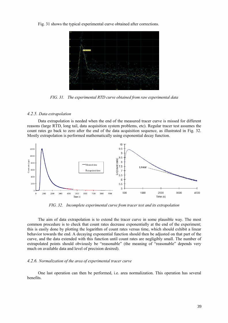
Fig. 31 shows the typical experimental curve obtained after corrections.

FIG. 31. The experimental RTD curve obtained from raw experimental data

4.2.5. Data extrapolation

Data extrapolation is needed when the end of the measured tracer curve is missed for different reasons (large RTD, long tail, data acquisition system problems, etc). Regular tracer test assumes the count rates go back to zero after the end of the data acquisition sequence, as illustrated in Fig. 32. Mostly extrapolation is performed mathematically using exponential decay function.

FIG. 32. Incomplete experimental curve from tracer test and its extrapolation

The aim of data extrapolation is to extend the tracer curve in some plausible way. The most

common procedure is to check that count rates decrease exponentially at the end of the experiment; this is easily done by plotting the logarithm of count rates versus time, which should exhibit a linear behavior towards the end. A decaying exponential function should then be adjusted on that part of the curve, and the data extended with this function until count rates are negligibly small. The number of extrapolated points should obviously be “reasonable” (the meaning of “reasonable” depends very much on available data and level of precision desired).

4.2.6. Normalization of the area of experimental tracer curve

One last operation can then be performed, i.e. area normalization. This operation has several

benefits.

39

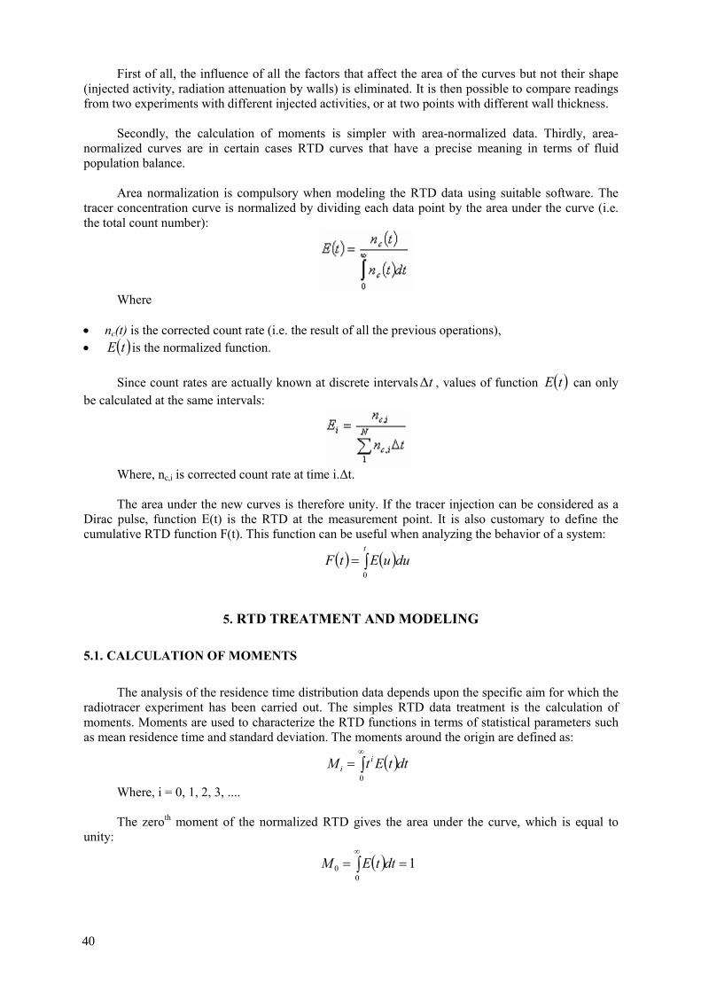
First of all, the influence of all the factors that affect the area of the curves but not their shape (injected activity, radiation attenuation by walls) is eliminated. It is then possible to compare readings from two experiments with different injected activities, or at two points with different wall thickness.

Secondly, the calculation of moments is simpler with area-normalized data. Thirdly, area-

normalized curves are in certain cases RTD curves that have a precise meaning in terms of fluid population balance.

Area normalization is compulsory when modeling the RTD data using suitable software. The

tracer concentration curve is normalized by dividing each data point by the area under the curve (i.e. the total count number):

Where

• nc(t) is the corrected count rate (i.e. the result of all the previous operations), • ( )tE is the normalized function.

Since count rates are actually known at discrete intervals tΔ , values of function ( )tE can only

be calculated at the same intervals:

Where, nc,i is corrected count rate at time i.Δt. The area under the new curves is therefore unity. If the tracer injection can be considered as a

Dirac pulse, function E(t) is the RTD at the measurement point. It is also customary to define the cumulative RTD function F(t). This function can be useful when analyzing the behavior of a system:

( ) ( )∫=t

duuEtF0

5. RTD TREATMENT AND MODELING

5.1. CALCULATION OF MOMENTS

The analysis of the residence time distribution data depends upon the specific aim for which the

radiotracer experiment has been carried out. The simples RTD data treatment is the calculation of moments. Moments are used to characterize the RTD functions in terms of statistical parameters such as mean residence time and standard deviation. The moments around the origin are defined as:

( )∫∞

=0

dttEtM ii

Where, i = 0, 1, 2, 3, .... The zeroth moment of the normalized RTD gives the area under the curve, which is equal to

unity:

( )∫∞

==0

0 1dttEM

40

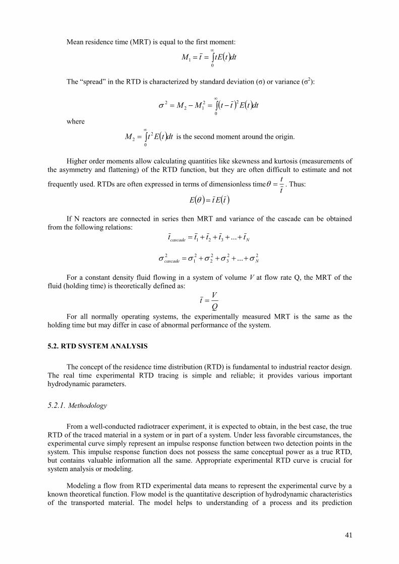
Mean residence time (MRT) is equal to the first moment:

( )∫∞

==0

1 dttEttM

The “spread” in the RTD is characterized by standard deviation (σ) or variance (σ2):

( ) ( )∫∞

−=−=0

2212

2 dttEttMMσ

where

( )∫∞

=0

22 dttEtM is the second moment around the origin.

Higher order moments allow calculating quantities like skewness and kurtosis (measurements of

the asymmetry and flattening) of the RTD function, but they are often difficult to estimate and not

frequently used. RTDs are often expressed in terms of dimensionless timett

=θ . Thus:

( ) ( )tEtE =θ If N reactors are connected in series then MRT and variance of the cascade can be obtained

from the following relations: Ncascade ttttt ++++= ...321

22

322

21

2 ... Ncascade σσσσσ ++++= For a constant density fluid flowing in a system of volume V at flow rate Q, the MRT of the

fluid (holding time) is theoretically defined as:

QVt =

For all normally operating systems, the experimentally measured MRT is the same as the holding time but may differ in case of abnormal performance of the system.

5.2. RTD SYSTEM ANALYSIS

The concept of the residence time distribution (RTD) is fundamental to industrial reactor design.

The real time experimental RTD tracing is simple and reliable; it provides various important hydrodynamic parameters.

5.2.1. Methodology

From a well-conducted radiotracer experiment, it is expected to obtain, in the best case, the true

RTD of the traced material in a system or in part of a system. Under less favorable circumstances, the experimental curve simply represent an impulse response function between two detection points in the system. This impulse response function does not possess the same conceptual power as a true RTD, but contains valuable information all the same. Appropriate experimental RTD curve is crucial for system analysis or modeling.

Modeling a flow from RTD experimental data means to represent the experimental curve by a

known theoretical function. Flow model is the quantitative description of hydrodynamic characteristics of the transported material. The model helps to understanding of a process and its prediction

41

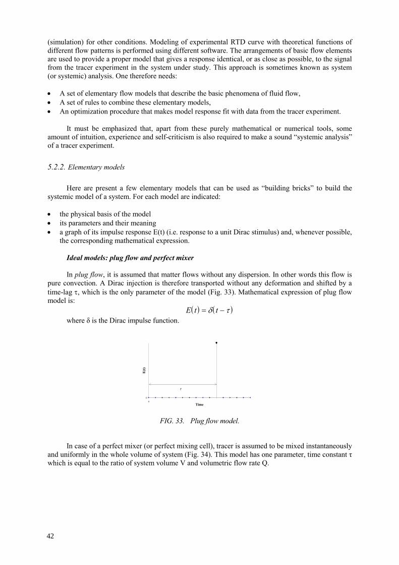
(simulation) for other conditions. Modeling of experimental RTD curve with theoretical functions of different flow patterns is performed using different software. The arrangements of basic flow elements are used to provide a proper model that gives a response identical, or as close as possible, to the signal from the tracer experiment in the system under study. This approach is sometimes known as system (or systemic) analysis. One therefore needs:

• A set of elementary flow models that describe the basic phenomena of fluid flow, • A set of rules to combine these elementary models, • An optimization procedure that makes model response fit with data from the tracer experiment.

It must be emphasized that, apart from these purely mathematical or numerical tools, some

amount of intuition, experience and self-criticism is also required to make a sound “systemic analysis” of a tracer experiment.

5.2.2. Elementary models

Here are present a few elementary models that can be used as “building bricks” to build the

systemic model of a system. For each model are indicated:

• the physical basis of the model • its parameters and their meaning • a graph of its impulse response E(t) (i.e. response to a unit Dirac stimulus) and, whenever possible,

the corresponding mathematical expression. Ideal models: plug flow and perfect mixer In plug flow, it is assumed that matter flows without any dispersion. In other words this flow is

pure convection. A Dirac injection is therefore transported without any deformation and shifted by a time-lag τ, which is the only parameter of the model (Fig. 33). Mathematical expression of plug flow model is:

( ) ( )E t t= −δ τ where δ is the Dirac impulse function.

00

Time

E(t

)

τ

FIG. 33. Plug flow model.

In case of a perfect mixer (or perfect mixing cell), tracer is assumed to be mixed instantaneously

and uniformly in the whole volume of system (Fig. 34). This model has one parameter, time constant τ which is equal to the ratio of system volume V and volumetric flow rate Q.

42

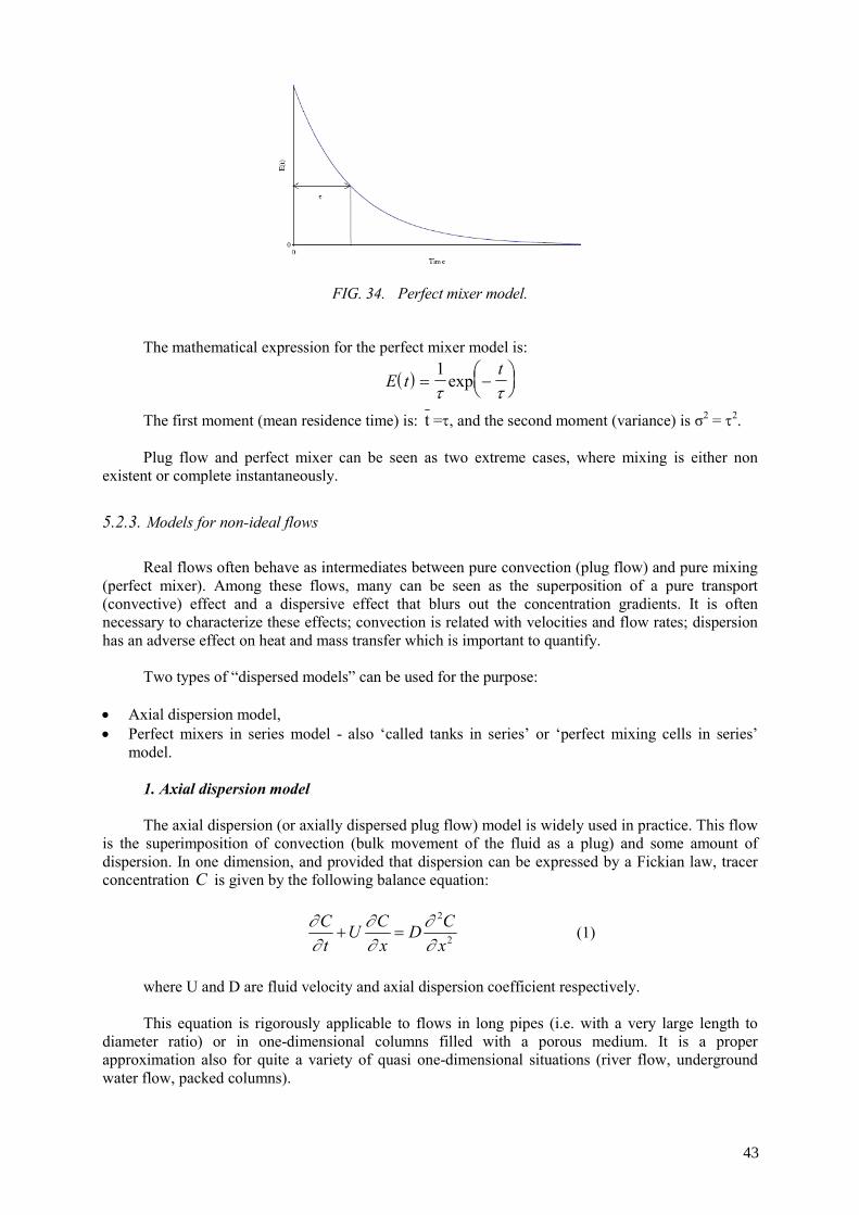
FIG. 34. Perfect mixer model.

The mathematical expression for the perfect mixer model is:

( )E tt

= −⎛⎝⎜

⎞⎠⎟

1τ τ

exp

The first moment (mean residence time) is: t =τ, and the second moment (variance) is σ2 = τ2. Plug flow and perfect mixer can be seen as two extreme cases, where mixing is either non

existent or complete instantaneously.

5.2.3. Models for non-ideal flows

Real flows often behave as intermediates between pure convection (plug flow) and pure mixing

(perfect mixer). Among these flows, many can be seen as the superposition of a pure transport (convective) effect and a dispersive effect that blurs out the concentration gradients. It is often necessary to characterize these effects; convection is related with velocities and flow rates; dispersion has an adverse effect on heat and mass transfer which is important to quantify.

Two types of “dispersed models” can be used for the purpose:

• Axial dispersion model, • Perfect mixers in series model - also ‘called tanks in series’ or ‘perfect mixing cells in series’

model.

1. Axial dispersion model The axial dispersion (or axially dispersed plug flow) model is widely used in practice. This flow

is the superimposition of convection (bulk movement of the fluid as a plug) and some amount of dispersion. In one dimension, and provided that dispersion can be expressed by a Fickian law, tracer concentration C is given by the following balance equation:

2

2

xCD

xCU

tC

∂∂

∂∂

∂∂

=+ (1)

where U and D are fluid velocity and axial dispersion coefficient respectively. This equation is rigorously applicable to flows in long pipes (i.e. with a very large length to

diameter ratio) or in one-dimensional columns filled with a porous medium. It is a proper approximation also for quite a variety of quasi one-dimensional situations (river flow, underground water flow, packed columns).

43

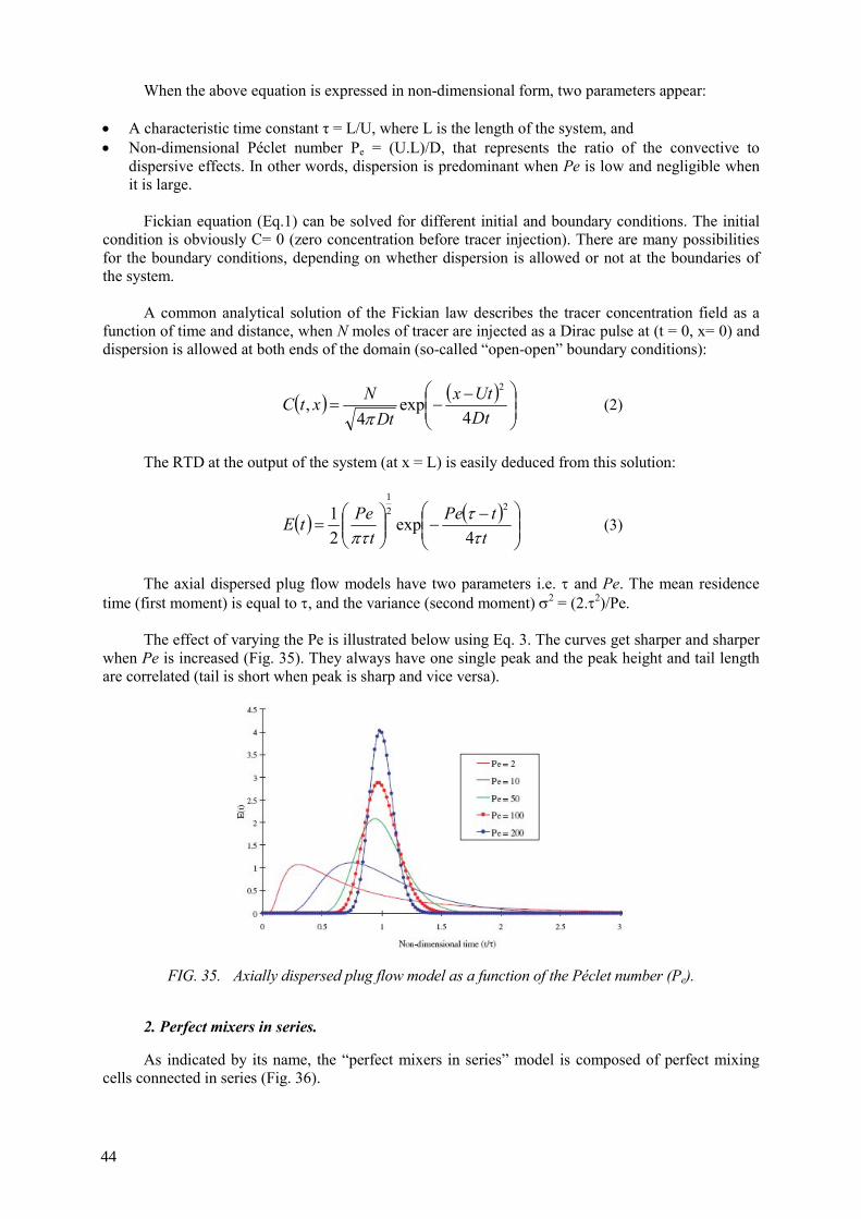
When the above equation is expressed in non-dimensional form, two parameters appear:

• A characteristic time constant τ = L/U, where L is the length of the system, and • Non-dimensional Péclet number Pe = (U.L)/D, that represents the ratio of the convective to

dispersive effects. In other words, dispersion is predominant when Pe is low and negligible when it is large.

Fickian equation (Eq.1) can be solved for different initial and boundary conditions. The initial

condition is obviously C= 0 (zero concentration before tracer injection). There are many possibilities for the boundary conditions, depending on whether dispersion is allowed or not at the boundaries of the system.

A common analytical solution of the Fickian law describes the tracer concentration field as a

function of time and distance, when N moles of tracer are injected as a Dirac pulse at (t = 0, x= 0) and dispersion is allowed at both ends of the domain (so-called “open-open” boundary conditions):

( ) ( )⎟⎟⎠

⎞⎜⎜⎝

⎛ −−=

DtUtx

tDNxtC

4exp

4,

2

π (2)

The RTD at the output of the system (at x = L) is easily deduced from this solution:

( ) ( )⎟⎟⎠

⎞⎜⎜⎝

⎛ −−⎟⎟

⎠

⎞⎜⎜⎝

⎛=

ttPe

tPetE

ττ

τπ 4exp

21 22

1

(3)

The axial dispersed plug flow models have two parameters i.e. τ and Pe. The mean residence

time (first moment) is equal to τ, and the variance (second moment) σ2 = (2.τ2)/Pe. The effect of varying the Pe is illustrated below using Eq. 3. The curves get sharper and sharper

when Pe is increased (Fig. 35). They always have one single peak and the peak height and tail length are correlated (tail is short when peak is sharp and vice versa).

FIG. 35. Axially dispersed plug flow model as a function of the Péclet number (Pe).

2. Perfect mixers in series. As indicated by its name, the “perfect mixers in series” model is composed of perfect mixing

cells connected in series (Fig. 36).

44

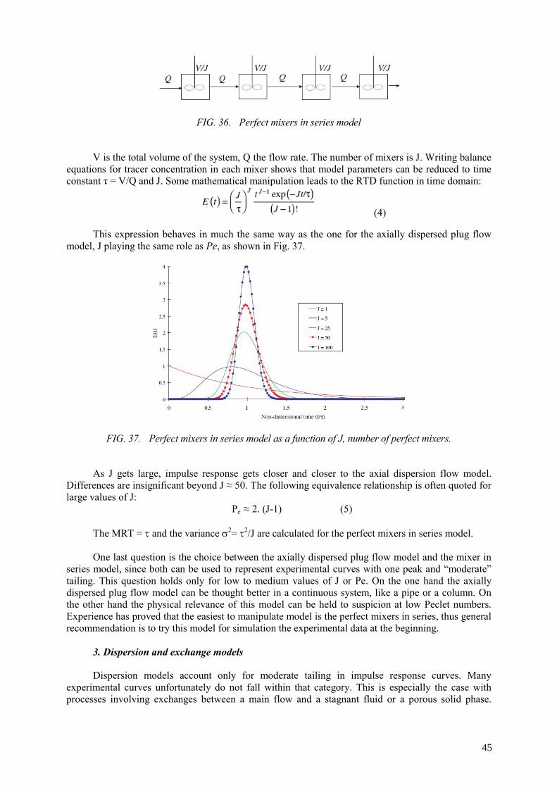
FIG. 36. Perfect mixers in series model

V is the total volume of the system, Q the flow rate. The number of mixers is J. Writing balance

equations for tracer concentration in each mixer shows that model parameters can be reduced to time constant τ = V/Q and J. Some mathematical manipulation leads to the RTD function in time domain:

(4) This expression behaves in much the same way as the one for the axially dispersed plug flow

model, J playing the same role as Pe, as shown in Fig. 37.

FIG. 37. Perfect mixers in series model as a function of J, number of perfect mixers.

As J gets large, impulse response gets closer and closer to the axial dispersion flow model.

Differences are insignificant beyond J ≈ 50. The following equivalence relationship is often quoted for large values of J:

Pe ≈ 2. (J-1) (5) The MRT = τ and the variance σ2= τ2/J are calculated for the perfect mixers in series model. One last question is the choice between the axially dispersed plug flow model and the mixer in

series model, since both can be used to represent experimental curves with one peak and “moderate” tailing. This question holds only for low to medium values of J or Pe. On the one hand the axially dispersed plug flow model can be thought better in a continuous system, like a pipe or a column. On the other hand the physical relevance of this model can be held to suspicion at low Peclet numbers. Experience has proved that the easiest to manipulate model is the perfect mixers in series, thus general recommendation is to try this model for simulation the experimental data at the beginning.

3. Dispersion and exchange models Dispersion models account only for moderate tailing in impulse response curves. Many

experimental curves unfortunately do not fall within that category. This is especially the case with processes involving exchanges between a main flow and a stagnant fluid or a porous solid phase.

45

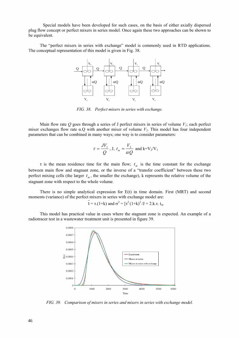
Special models have been developed for such cases, on the basis of either axially dispersed plug flow concept or perfect mixers in series model. Once again these two approaches can be shown to be equivalent.

The “perfect mixers in series with exchange” model is commonly used in RTD applications.

The conceptual representation of this model is given in Fig. 38.

FIG. 38. Perfect mixers in series with exchange.

Main flow rate Q goes through a series of J perfect mixers in series of volume V1; each perfect

mixer exchanges flow rate α.Q with another mixer of volume V2. This model has four independent parameters that can be combined in many ways; one way is to consider parameters:

QJV1=τ , J,

QV

tm α2= and k=V2/V1

τ is the mean residence time for the main flow; tm is the time constant for the exchange

between main flow and stagnant zone, or the inverse of a “transfer coefficient” between these two perfect mixing cells (the larger tm , the smaller the exchange), k represents the relative volume of the stagnant zone with respect to the whole volume.

There is no simple analytical expression for E(t) in time domain. First (MRT) and second

moments (variance) of the perfect mixers in series with exchange model are: t = τ.(1+k) and σ2 = [τ2 (1+k)2 /J + 2.k.τ. tm

This model has practical value in cases where the stagnant zone is expected. An example of a

radiotracer test in a wastewater treatment unit is presented in figure 39.

FIG. 39. Comparison of mixers in series and mixers in series with exchange model.

46

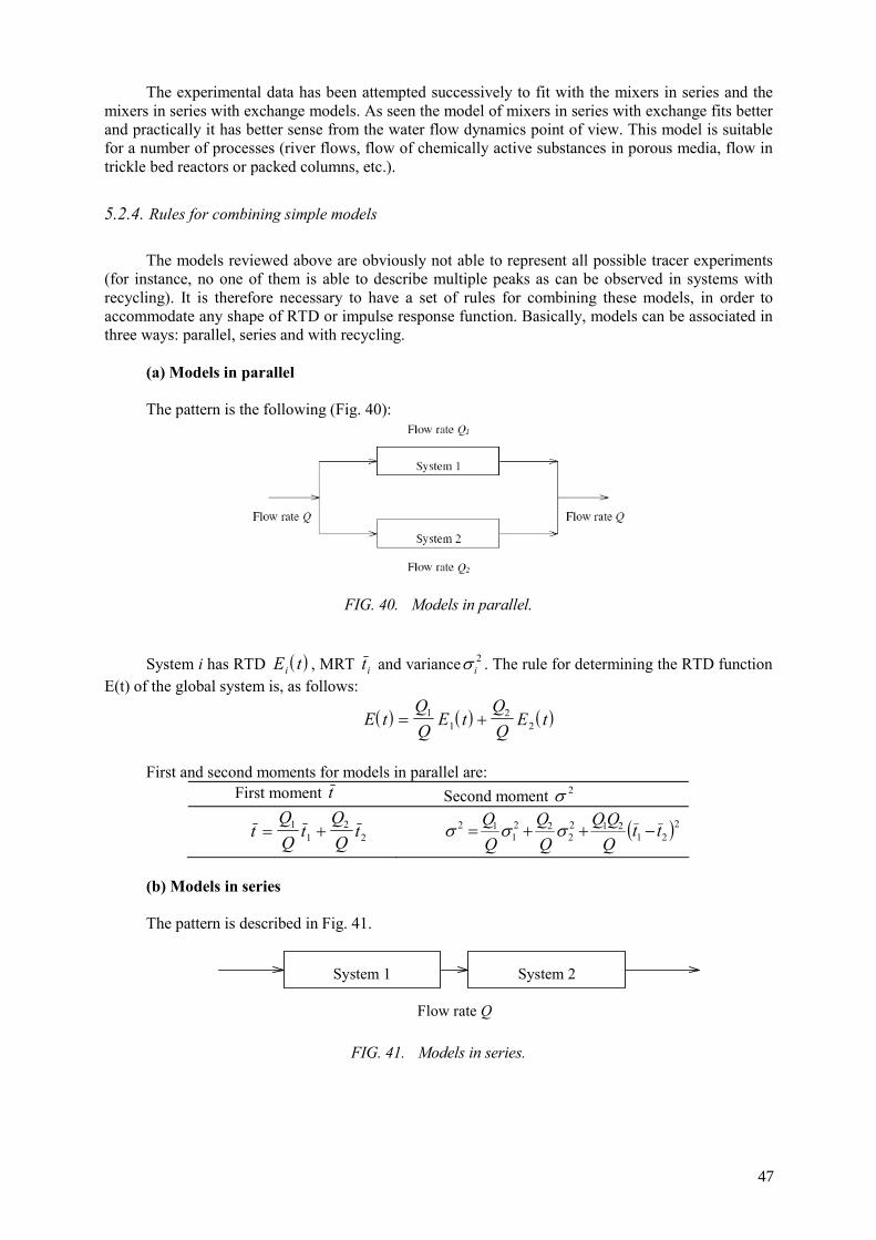
The experimental data has been attempted successively to fit with the mixers in series and the mixers in series with exchange models. As seen the model of mixers in series with exchange fits better and practically it has better sense from the water flow dynamics point of view. This model is suitable for a number of processes (river flows, flow of chemically active substances in porous media, flow in trickle bed reactors or packed columns, etc.).

5.2.4. Rules for combining simple models

The models reviewed above are obviously not able to represent all possible tracer experiments

(for instance, no one of them is able to describe multiple peaks as can be observed in systems with recycling). It is therefore necessary to have a set of rules for combining these models, in order to accommodate any shape of RTD or impulse response function. Basically, models can be associated in three ways: parallel, series and with recycling.

(a) Models in parallel The pattern is the following (Fig. 40):

FIG. 40. Models in parallel.

System i has RTD ( )E ti , MRT ti and varianceσ i

2 . The rule for determining the RTD function E(t) of the global system is, as follows:

( ) ( ) ( )E tQQ

E tQQ

E t= +11

22

First and second moments for models in parallel are:

First moment t Second moment σ 2

tQQ

tQQ

t= +11

22 ( )221

2122

221

12 ttQQQ

QQ

QQ

−++= σσσ

(b) Models in series The pattern is described in Fig. 41.

System 1 System 2

Flow rate Q

FIG. 41. Models in series.

47

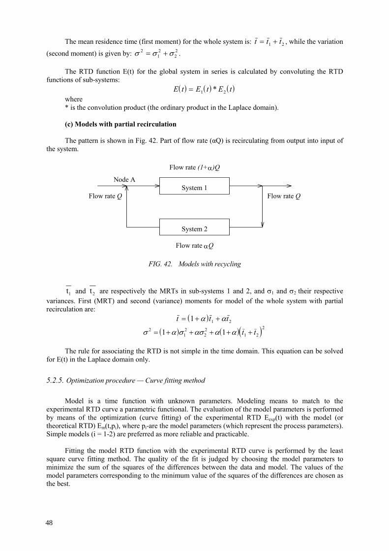
The mean residence time (first moment) for the whole system is: t t t= +1 2 , while the variation

(second moment) is given by: σ σ σ212

22= + .

The RTD function E(t) for the global system in series is calculated by convoluting the RTD

functions of sub-systems: ( ) ( ) ( )E t E t E t= 1 2*

where * is the convolution product (the ordinary product in the Laplace domain). (c) Models with partial recirculation The pattern is shown in Fig. 42. Part of flow rate (αQ) is recirculating from output into input of

the system.

System 1

System 2

Flow rate Q

Flow rate αQ

Flow rate (1+α)Q

Flow rate Q

Node A

FIG. 42. Models with recycling

1t and 2t are respectively the MRTs in sub-systems 1 and 2, and σ1 and σ2 their respective variances. First (MRT) and second (variance) moments for model of the whole system with partial recirculation are:

( )t t t= + +1 1 2α α

( ) ( )( )σ α σ ασ α α212

22

1 2

21 1= + + + + +t t

The rule for associating the RTD is not simple in the time domain. This equation can be solved

for E(t) in the Laplace domain only.

5.2.5. Optimization procedure — Curve fitting method

Model is a time function with unknown parameters. Modeling means to match to the

experimental RTD curve a parametric functional. The evaluation of the model parameters is performed by means of the optimization (curve fitting) of the experimental RTD Eexp(t) with the model (or theoretical RTD) Em(t,pi), where pi-are the model parameters (which represent the process parameters). Simple models (i = 1-2) are preferred as more reliable and practicable.

Fitting the model RTD function with the experimental RTD curve is performed by the least

square curve fitting method. The quality of the fit is judged by choosing the model parameters to minimize the sum of the squares of the differences between the data and model. The values of the model parameters corresponding to the minimum value of the squares of the differences are chosen as the best.

48

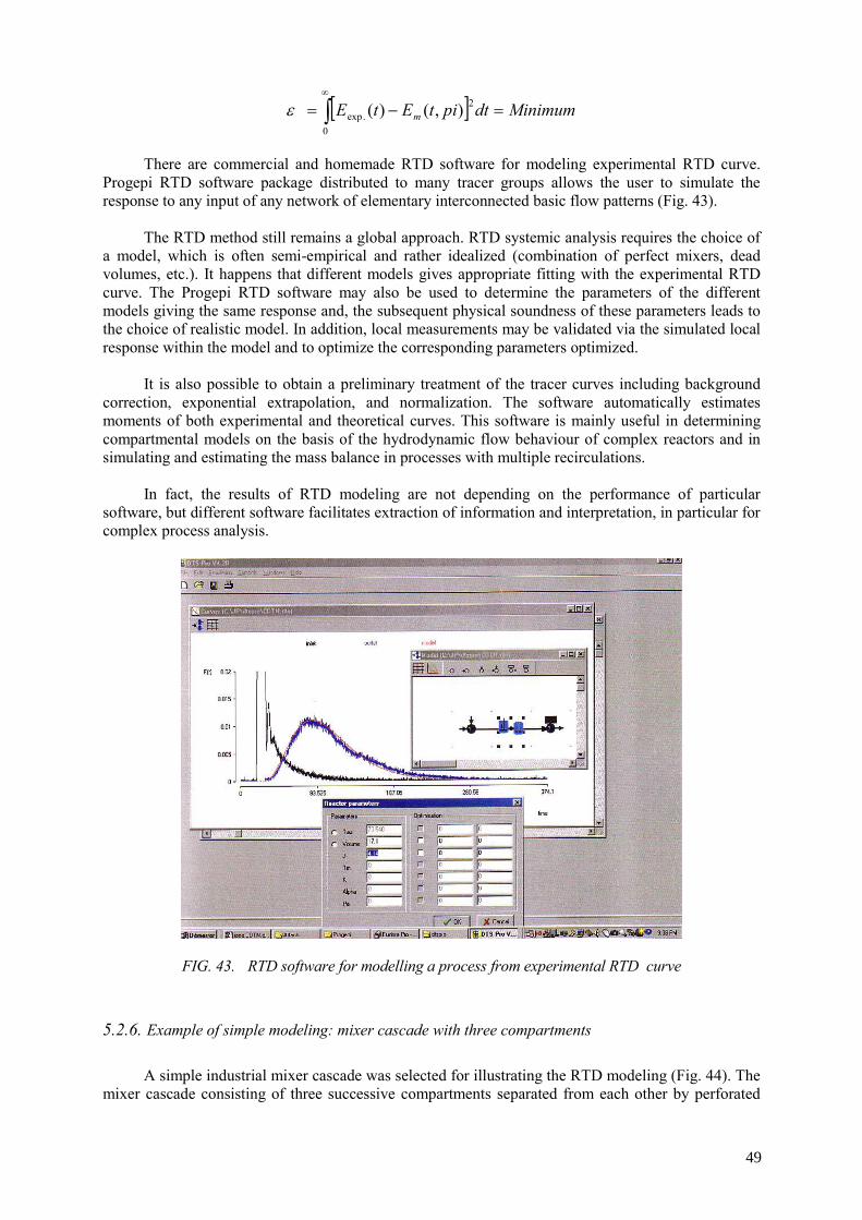
[ ] MinimumdtpitEtE m =−= ∫∞

0

2.exp ),()(ε

There are commercial and homemade RTD software for modeling experimental RTD curve.

Progepi RTD software package distributed to many tracer groups allows the user to simulate the response to any input of any network of elementary interconnected basic flow patterns (Fig. 43).

The RTD method still remains a global approach. RTD systemic analysis requires the choice of

a model, which is often semi-empirical and rather idealized (combination of perfect mixers, dead volumes, etc.). It happens that different models gives appropriate fitting with the experimental RTD curve. The Progepi RTD software may also be used to determine the parameters of the different models giving the same response and, the subsequent physical soundness of these parameters leads to the choice of realistic model. In addition, local measurements may be validated via the simulated local response within the model and to optimize the corresponding parameters optimized.

It is also possible to obtain a preliminary treatment of the tracer curves including background correction, exponential extrapolation, and normalization. The software automatically estimates moments of both experimental and theoretical curves. This software is mainly useful in determining compartmental models on the basis of the hydrodynamic flow behaviour of complex reactors and in simulating and estimating the mass balance in processes with multiple recirculations.

In fact, the results of RTD modeling are not depending on the performance of particular

software, but different software facilitates extraction of information and interpretation, in particular for complex process analysis.

FIG. 43. RTD software for modelling a process from experimental RTD curve

5.2.6. Example of simple modeling: mixer cascade with three compartments

A simple industrial mixer cascade was selected for illustrating the RTD modeling (Fig. 44). The

mixer cascade consisting of three successive compartments separated from each other by perforated

49

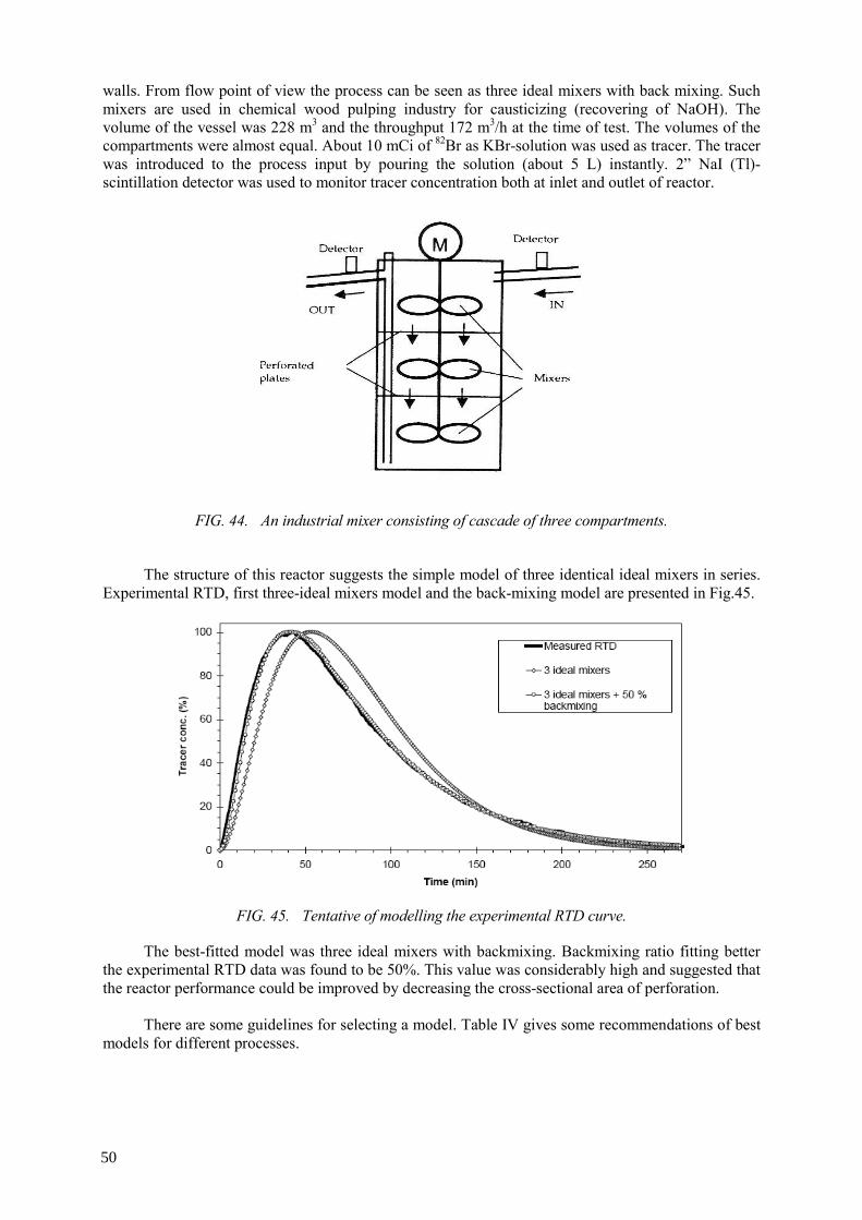
walls. From flow point of view the process can be seen as three ideal mixers with back mixing. Such mixers are used in chemical wood pulping industry for causticizing (recovering of NaOH). The volume of the vessel was 228 m3 and the throughput 172 m3/h at the time of test. The volumes of the compartments were almost equal. About 10 mCi of 82Br as KBr-solution was used as tracer. The tracer was introduced to the process input by pouring the solution (about 5 L) instantly. 2” NaI (Tl)- scintillation detector was used to monitor tracer concentration both at inlet and outlet of reactor.

FIG. 44. An industrial mixer consisting of cascade of three compartments.

The structure of this reactor suggests the simple model of three identical ideal mixers in series.

Experimental RTD, first three-ideal mixers model and the back-mixing model are presented in Fig.45.

FIG. 45. Tentative of modelling the experimental RTD curve.

The best-fitted model was three ideal mixers with backmixing. Backmixing ratio fitting better the experimental RTD data was found to be 50%. This value was considerably high and suggested that the reactor performance could be improved by decreasing the cross-sectional area of perforation.

There are some guidelines for selecting a model. Table IV gives some recommendations of best

models for different processes.

50

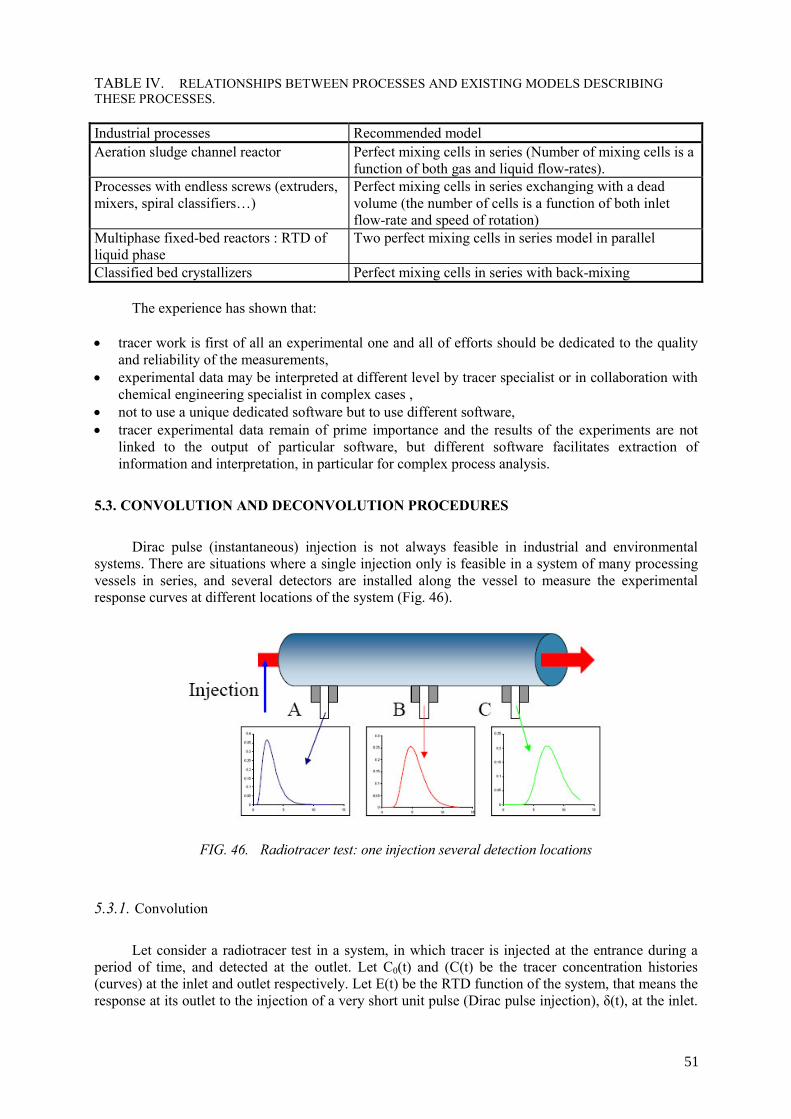
TABLE IV. RELATIONSHIPS BETWEEN PROCESSES AND EXISTING MODELS DESCRIBING THESE PROCESSES.

Industrial processes Recommended model Aeration sludge channel reactor Perfect mixing cells in series (Number of mixing cells is a

function of both gas and liquid flow-rates). Processes with endless screws (extruders, mixers, spiral classifiers…)

Perfect mixing cells in series exchanging with a dead volume (the number of cells is a function of both inlet flow-rate and speed of rotation)

Multiphase fixed-bed reactors : RTD of liquid phase

Two perfect mixing cells in series model in parallel

Classified bed crystallizers Perfect mixing cells in series with back-mixing

The experience has shown that:

• tracer work is first of all an experimental one and all of efforts should be dedicated to the quality and reliability of the measurements,

• experimental data may be interpreted at different level by tracer specialist or in collaboration with chemical engineering specialist in complex cases ,

• not to use a unique dedicated software but to use different software, • tracer experimental data remain of prime importance and the results of the experiments are not

linked to the output of particular software, but different software facilitates extraction of information and interpretation, in particular for complex process analysis.

5.3. CONVOLUTION AND DECONVOLUTION PROCEDURES

Dirac pulse (instantaneous) injection is not always feasible in industrial and environmental

systems. There are situations where a single injection only is feasible in a system of many processing vessels in series, and several detectors are installed along the vessel to measure the experimental response curves at different locations of the system (Fig. 46).

FIG. 46. Radiotracer test: one injection several detection locations

5.3.1. Convolution

Let consider a radiotracer test in a system, in which tracer is injected at the entrance during a

period of time, and detected at the outlet. Let C0(t) and (C(t) be the tracer concentration histories (curves) at the inlet and outlet respectively. Let E(t) be the RTD function of the system, that means the response at its outlet to the injection of a very short unit pulse (Dirac pulse injection), δ(t), at the inlet.

51

Convolution is the mathematical transformation that allows to predict the response to any injection history C0(t) from the known E(t).

Taking advantage of the linearity of the system, it is possible to express the response to the

whole injection sequence Co(t) as the sum of the responses to each individual injection step. In other words, signal at the outlet can be written as:

( ) ( ) ( )∫∞

−=0

0 duutEuCtC

which expresses that C(t) is the convolution product of Co(t) and E(t), often noted as C0*E. Decomposition of Co(t) into multiple steps, calculation of response to each step, summation of the responses) are illustrated in Fig. 47.

Several mathematical methods can be used to resolve convolution or deconvolution problems:

• direct numerical calculation (time domain or Fourier transform) • correlation techniques • optimisation techniques

Experience has shown that simple methods always work for convolution but they usually fail for

deconvolution. There are many software solving the convolution or deconvolution operations, thus not going into details of mathematical operations we recommend to the reader just to make use of these software.

FIG. 47. Principle of convolution method

Convolution is not much used in real tracer applications, because the main problem of tracer

method is to identify and quantify the residence time distribution (RTD) function that means to determine the model of the process and to find its parameters. Normally, during a radiotracer test the experiental response curves are recorded at the inlet and outlet of the system, thus the C0(t) and C(t) are known. The most often problem is to find the E(t) from C0(t) and C(t). This is so called the deconvolution operation.

52

5.3.2. Deconvolution

Convolution consists in calculating C(t) when C0(t) and E(t) are known. Deconvolution is the

inverse procedure, i.e. calculation of E(t) when C0(t) and C(t) are known. This case, where responses at two measurement stations are known, is being the most common one in tracer applications. The deconvolution of C(t) and Co(t) is noted as: C/Co, keeping in mind that if convolution is commutative, deconvolution is not.

There are several reasons why one needs to deconvolute signals. Any stationary and linear

system is unambiguously characterized by its impulse response function, or its response to a Dirac pulse stimulus. This response can, in most practical cases, be considered as the RTD of the traced material. Knowledge of that impulse response function is therefore desirable to be able to predict system response to any stimulus, or to analyze system behaviour in terms of RTD. Unfortunately, injection of a true Dirac pulse of tracer is not always achievable. Besides, it is quite common to have several detectors at different stages of complex systems. Even if tracer is injected as a perfect Dirac pulse, only readings from the first detector can be considered as the impulse response function of that part of the system; one has to deconvolute the signals from the second and first detectors (i.e. calculate

12 CC ÷ ) to get the impulse response function of the second part of the system, and so forth with the next detectors.

6. PLANNING AND EXECUTION OF A RADIOTRACER EXPERIMENT

Injecting a compatible radiotracer into an appropriate inlet upstream of a vessel and monitoring

its passage through the vessel allows RTD of fluid to be measured. Sensitive radiation detectors are placed at strategic elevations / locations on the vessel. The detectors are relatively small and easy to mount at each position. Each one is connected by a cable to a central data logging device that records radiotracer concentration versus time information. When the radiotracer passes each detector a response is registered and recorded. Prior to the test each detector is assessed and its response normalized such that each detector responds identically to a given unit of radiotracer.

The success of a RTD experiment depends upon proper planning, execution and mode of

analysis of the obtained data. The accurate measurement of the RTD experimental curve is crucial for further processing and interpretation. The experimental RTD curve can be obtained either by online measurement of the radioactivity, or by sampling and subsequently measurement in laboratory.

6.1. AMOUNT OF ACTIVITY

6.1.1. Factors influencing the radiotracer activity

The most frequently asked question is: How much activity is needed in order to obtain a defined accuracy in measuring the experimental RTD curve? The amount of radiotracer required for a RTD test depends on the following factors:

• Accuracy • Efficiency of radiation detection system • Expected level of dilution/dispersion • Half life of radiotracer used • Background radiation level

53

Error (accuracy or uncertainty) is given by the standard deviation of the intensity of radiation. By experience, 5-10 % error is acceptable in online experiments. Off-line experiments, where samples are taken for counting, normally offers lower uncertainty (2-3 %).

6.1.2. Estimation of radiotracer activity for RTD tests

In continuous flow measurements the activity of radiotracer depends of the flow model. This

means that a preliminary model has to be selected based on the process consideration. Axial dispersion and tank-in-series models are two simple and commonly used models to characterize the flow behavior in industrial and hydrological systems.

a. Activity estimation using axial dispersion flow model First approach is based on the general model of the fluid flow, which takes account the axial

dispersion of tracer moving together with traced fluid. This approach is generally useful for estimation of amount of radiotracer for plug flow systems such as tubular reactors, trickle and packed bed columns. As mentioned above the RTD function for the axial dispersion model is:

( ) ( )⎟⎟⎠

⎞⎜⎜⎝

⎛ −−⎟⎟

⎠

⎞⎜⎜⎝

⎛=

ttPe

tPetE

ττ

τπ 4exp

21 22

1

where, mean residence time, τ = V/Q.

The maximum concentration (peak value) of tracer is obtained for t = τ and is given as: 2/1

.max /4),( ⎥⎦

⎤⎢⎣⎡=

τπtPe

VAtxC = A/V (Pe/4π)1/2

and:

A = Cmax .V. [2π1/2 / Pe1/2 ] = (3.545/Pe

1/2 )x Cmax .V Where: A is the radiotracer activity distributed uniformly in V volume of the reactor. The above equation can be used to estimate the amount of activity required for studying a

continuous flow reactor assuming the different values of the model parameter (D or Pe).

Example: A fluid flows in a reactor with a flow rate Q = 50 m3/min. An amount A of radiotracer was injected instantaneously into the inlet (at location x = 0 at time t = 0) and monitored at the reactor outlet. The volume (V) of the test reactor was 300 m3 and an accuracy of 5% imposes the requirement of the tracer concentration C max =50 μCi/m3 at the time t = τ at the detection point at the outlet. The calibration factor of the detector for the particular detection geometry used was found 1000 cpm/μCi/m3 (from the laboratory calibration). The flow pattern was supposed to approach the axial-dispersion model.

Let’s calculate the amount of the radiotracer required for a RTD test for different mixing rates.

Of course the amount of tracer required for a RTD test depends how much the cloud is dispersed along the pipe axe. It may be estimated as follows:

• Case 1: Let assume that the flow pattern in the pipeline is plug flow with Peclet Number (Pe)

equal to 100. The amount of activity required to be injected is estimated to be 197 MBq (5.3 mCi). • Case 2: Let consider the flow pattern be axially dispersed type i.e. the value of Pe is about 10,

then the activity estimated for this case is 622 MBq (16.8 mCi).

54

• Case 3: Now let assume that the flow pattern is well-mixed type that implies that the value of Pe is low. Let us say that the value of Pe is equal to 2, then the amount of activity is estimated to be 1391 MBq (37.6 mCi).

It is evident that higher axial mixing rate greater is the radiotracer activity to be injected for the

same accuracy. In the case of well mixed radiotracer the calculated required activity results nearly seven times more than for plug flow movement (no axial dispersion).

b. Activity estimation using tanks in series flow model Similarly the tank-in-series model description of the system could also be used for the

estimation of amount of radiotracer. The normalized RTD function in this case is:

The maximum concentration (peak value) of tracer is obtained at t = τ (θ = 1) and is given as:

Cmax (x,t) = (A/V) . {[JJ/(J-1)!]. exp (-J)} or the activity: A = Cmax V {[(J-1)!]/ JJ } eJ Now using the data of the previous example the amount of activity for the three different cases

that is J = 50 (plug flow pattern), J = 5 (axially dispersed pattern) and J = 1 (well-mixed pattern) was estimated to be 196 MBq (5.3 mCi), 633 MBq (17.1 mCi) and 1510 MBq (40.8 mCi) respectively. It seems that two models give similar estimations. The axial dispersion model is recommended to be used for low dispersion flows, while the tanks in series model for high dispersion flows.

6.2. IMPLEMENTATION OF THE RTD TEST

Equipment required for on-line tracer testing will depend upon the precise nature of the

undertaken work. It is recommended that a check list be prepared and items checked off before shipment. It will comprise the following:

• Suitable radioactive tracer • Suitable injection equipment • Suitable detecting and data acquisition systems • Radiation protection and safety instrument and tools .

Following steps are to be followed for implementing a radiotracer experiment. a. Complete understanding of system, process and problem This includes:

• Properties of process material (phase, density, viscosity etc.) • Process parameters (flowrate, volume, pressure, temperature, expected MRT etc.) • Flow diagram of the process material • Expected degree of mixing • Choice of a suitable radiotracer technique.

55

b. Feasibility assessment Complete understanding of the system, process and problem is required to assess the feasibility

of carrying out the experiment. The feasibility assessment includes:

• Plant visit and discussion with plant engineers • Selection of suitable injection and detection locations • Measurement of background radiation level • Waste disposal • Usefulness and economic aspects.

c. Execution of radiotracer test The execution of the planning involves the following steps:

• Fabrication and testing of suitable injection system, collimators, water jackets • Calibration of the detection system • Irradiation of target in the nuclear reactor • Preparation of radiotracer, dilution, dispensing, labelling etc. • Packing of radiotracer and its transportation to the site • Installation of injection system, collimators and detectors at suitably selected locations • Background measurement radiation levels • Injection of tracer and its measurement • Radiation surveillance to be provided by Health Physicist • Waste disposal to a safe location and measurements of dose rate at various locations along the

system and to advise the plant operators accordingly. d. Checklist for radiotracer field test The equipment and material required for a field radiotracer experiment may vary experiment to

experiment. A checklist of the commonly used equipment and material is given below: A. Radiotracer B. Tracer injection system with compatible fitting and valves C. Detection system:

• Ratemeter/Scaler • Data acquisition system/Laptop PC • Scintillation detector • Connecting cables • Collimators • Detector cooling system • Batteries/Dry cell • Standard source • Lead sheets or bricks

D. Radiation handling equipment:

• Radiation survey meter • Personnel monitoring equipment such as TLD badges and pocket dosimeters • Tracer vial opener (Decaping tool) • Tracer vial holder • Cee-Vee tons (0.5 and 1 meter) • Polythene or plastic gloves

56

• Polythene bags • Polythene sheets • Absorbent sheets • Tissue paper • Wash bottle • Beakers • Duster • Additive tape

E. Miscellaneous items:

• Instrument repair kit • Decontamination kit • Dummy tracer vial etc.

F. Packing boxes After carrying out the tracer tests the data will be treated, and the findings relayed to the client.

These will be confirmed in a written report to the customer within 14 days or in such time as agreed between the two parties.

7. RESIDENCE TIME DISTRIBUTION APPLICATIONS

7.1. MAJOR TARGETS Stimulated by an ever increasing demand from the large production plants, many radiotracer

techniques have been evolved to provide fast and effective solutions to plant and process problems. These techniques are now in routine service to industry in many developed and developing countries. The number of services for troubleshooting inspections carried out per year is not known precisely, but it is certainly in excess of several thousand, worldwide. The services are available either from private companies, who carry out the majority of applications, or from national nuclear centres.

Relevant target areas for radiotracer residence time distribution (RTD) applications are defined.

Though the RTD technology is applicable across a broad industrial spectrum, the petroleum and petrochemical industries, mineral processing and waste-water treatment sectors are identified as the most appropriate target beneficiaries of radioisotope applications: these industries are widespread internationally and are of considerable economic and environmental importance. Residence time distribution measured by radiotracers has become an important tool for the diagnosis of industrial processing units. The major targets for applications of radiotracer RTD methods are:

a. Petroleum industry The applications of radiotracer RTD methods are widespread throughout oil refineries

worldwide and this industry is one of the main users, and beneficiaries of the technology. Economically, the most important operating unit in a refinery is the Fluidized Catalytic Cracking Unit (FCCU), the function of which is to upgrade the “heavy” components of the oil to gasoline. Technically, this is also the most complex unit, involving as it does the interaction of multiple phases: solid catalyst, vaporized feedstock steam and air. Because of the construction and extreme operating conditions of FCCUs, the only effective way to diagnose their behaviour is through the application of radiotracers.

Radioactive tracers have been used to great effect in enhancing oil production in oil fields. The

main radiotracer technique is the measuring of the “time of travel” between injection and production wells. If a water injection is to be effective in sweeping out oil from the permeable zones it is

57

important to ensure that short-circuiting or channelling, whereby much of the residual oil may be bypassed, does not occur. Therefore, it is important to understand how the water from injection well travels to the producer.

b. Petrochemical complexes The petrochemicals plant lies immediately downstream of the oil refinery and in many

developing countries construction of the two types of facility is proceeding in parallel. Like refineries, petrochemicals plants are generally continuously operating and technically complex. Thus, high economic benefits may be realized by the applications of radiotracer techniques on petrochemicals units.

Though radiotracer RTD methods are useful in solving a wide range of problems, the economic

benefits become more pronounced the further “upstream” they are applied. This means that diagnosis of the cracking furnace, primary fractionator and gas separation chain is of the highest potential value.

c. Minerals processing This generic heading covers an enormous range of industries. Minerals processing plants, in one

form or another are to be found in practically every country in the world, and in many cases they are major contributors to national economy. Though the range of minerals which are extracted and processed is extremely wide, there are certain processes found throughout the industry:

• Comminution • Classification • Flotation • Homogenization

d. Wastewater treatment ponds The primary justification for focusing attention on this sector is based upon health and

environmental considerations, rather than purely on economic benefits per se. The operation of a wastewater treatment lagoon can be deceptively complex. Given the unsatisfactory state of current theoretical approaches, there is a need to be able to assess performance practically; that is, by actually measuring the RTD. Modelling by RTD is a powerful tool, aiding both the design and performance optimization of wastewater treatment systems.

The benefits are:

• ensuring thorough treatment of waste-water thereby safeguarding the environment, • operating existing ponds more effectively- saving money, • providing data for the design of future ponds.

7.2. RTD FOR TROUBLESHOOTING

Residence time distribution (RTD) and mean residence time (MRT) and are two important

parameters of continuously operating industrial process systems, which have a direct bearing on process efficiency and product quality. The measured residence time distribution data are analyzed either to identify the cause of malfunctioning or to characterize the degree of mixing in the system. RTD technique using radiotracers has been routinely used to diagnose imperfect mixing.

There are a number of reasons for imperfect mixing, i.e. presence of dead (or stagnant) volume,

occurrence of channelling, split in parallel or preferential flows, bypass or short circuit exit flows and holding-up. These symptoms are reflected in the experimental response curves.

58

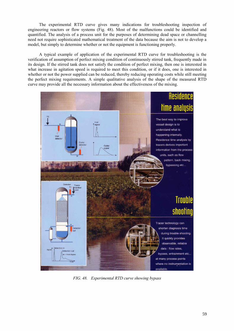
The experimental RTD curve gives many indications for troubleshooting inspection of engineering reactors or flow systems (Fig. 48). Most of the malfunctions could be identified and quantified. The analysis of a process unit for the purposes of determining dead space or channelling need not require sophisticated mathematical treatment of the data because the aim is not to develop a model, but simply to determine whether or not the equipment is functioning properly.

A typical example of application of the experimental RTD curve for troubleshooting is the

verification of assumption of perfect mixing condition of continuously stirred tank, frequently made in its design. If the stirred tank does not satisfy the condition of perfect mixing, then one is interested in what increase in agitation speed is required to meet this condition, or if it does, one is interested in whether or not the power supplied can be reduced, thereby reducing operating costs while still meeting the perfect mixing requirements. A simple qualitative analysis of the shape of the measured RTD curve may provide all the necessary information about the effectiveness of the mixing.

FIG. 48. Experimental RTD curve showing bypass

59

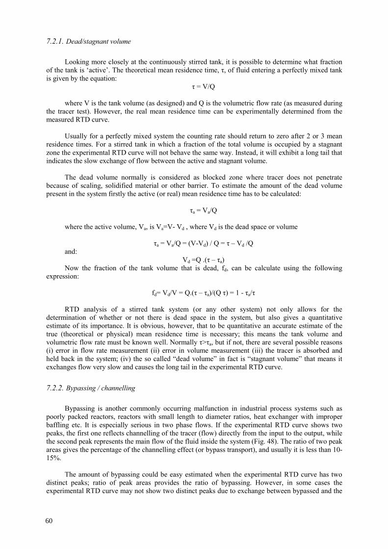
7.2.1. Dead/stagnant volume

Looking more closely at the continuously stirred tank, it is possible to determine what fraction

of the tank is ‘active’. The theoretical mean residence time, τ, of fluid entering a perfectly mixed tank is given by the equation:

τ = V/Q where V is the tank volume (as designed) and Q is the volumetric flow rate (as measured during

the tracer test). However, the real mean residence time can be experimentally determined from the measured RTD curve.

Usually for a perfectly mixed system the counting rate should return to zero after 2 or 3 mean

residence times. For a stirred tank in which a fraction of the total volume is occupied by a stagnant zone the experimental RTD curve will not behave the same way. Instead, it will exhibit a long tail that indicates the slow exchange of flow between the active and stagnant volume.

The dead volume normally is considered as blocked zone where tracer does not penetrate

because of scaling, solidified material or other barrier. To estimate the amount of the dead volume present in the system firstly the active (or real) mean residence time has to be calculated:

τa = Va/Q

where the active volume, Va, is Va=V- Vd , where Vd is the dead space or volume

τa = Va/Q = (V-Vd) / Q = τ – Vd /Q and:

Vd =Q .(τ – τa) Now the fraction of the tank volume that is dead, fd, can be calculate using the following

expression:

fd= Vd/V = Q.(τ – τa)/(Q τ) = 1 - τa/τ RTD analysis of a stirred tank system (or any other system) not only allows for the

determination of whether or not there is dead space in the system, but also gives a quantitative estimate of its importance. It is obvious, however, that to be quantitative an accurate estimate of the true (theoretical or physical) mean residence time is necessary; this means the tank volume and volumetric flow rate must be known well. Normally τ>τa, but if not, there are several possible reasons (i) error in flow rate measurement (ii) error in volume measurement (iii) the tracer is absorbed and held back in the system; (iv) the so called “dead volume” in fact is “stagnant volume” that means it exchanges flow very slow and causes the long tail in the experimental RTD curve.

7.2.2. Bypassing / channelling

Bypassing is another commonly occurring malfunction in industrial process systems such as

poorly packed reactors, reactors with small length to diameter ratios, heat exchanger with improper baffling etc. It is especially serious in two phase flows. If the experimental RTD curve shows two peaks, the first one reflects channelling of the tracer (flow) directly from the input to the output, while the second peak represents the main flow of the fluid inside the system (Fig. 48). The ratio of two peak areas gives the percentage of the channelling effect (or bypass transport), and usually it is less than 10-15%.

The amount of bypassing could be easy estimated when the experimental RTD curve has two

distinct peaks; ratio of peak areas provides the ratio of bypassing. However, in some cases the experimental RTD curve may not show two distinct peaks due to exchange between bypassed and the

60

main part of the fluid. In such cases, the cumulative RTD curve (F curve) could be useful for bypass detection. The initial rapidly increasing part of the cumulative F curve gives fraction of the bypassed fluid.

Experimental RTD curve might show two or more peaks depending on the fluid transport and

process characteristics. These peaks might represent parallel or preferential flows. Bypassing is considered only when comes first and fast (less than 10-15% of the MRT), and when its area consists of less than 10-15% of the main flow curve; while the amplitude of the bypassing peak might be higher or lower that the main flow peak.

7.3. RTD FOR DIAGNOSIS OF INDUSTRIAL PROCESSES: CASE STUDIES

A typical radiotracer test design for problem solving in a chemical engineering reactor is shown

FIG. 49. Solid and gas tracing in a waste incinerator facility, design of radiotracer test

7.3.1. Radiotracers for diagnosis of Fluid Catalytic Cracking (F.C.C.) units

In large scale plants, such as Fluid Catalytic Cracking Units (FCCU), even a small increase in

yield can bring significant gain in productivity and hence also in revenue. Fluid Catalytic Cracking is the most important and widely used process in petroleum refining for conversion of heavy oils into gasoline and lighter products (Fig. 50). Units designed to carry out this process are the economic heart of the refinery.

61

in the Fig. 49.

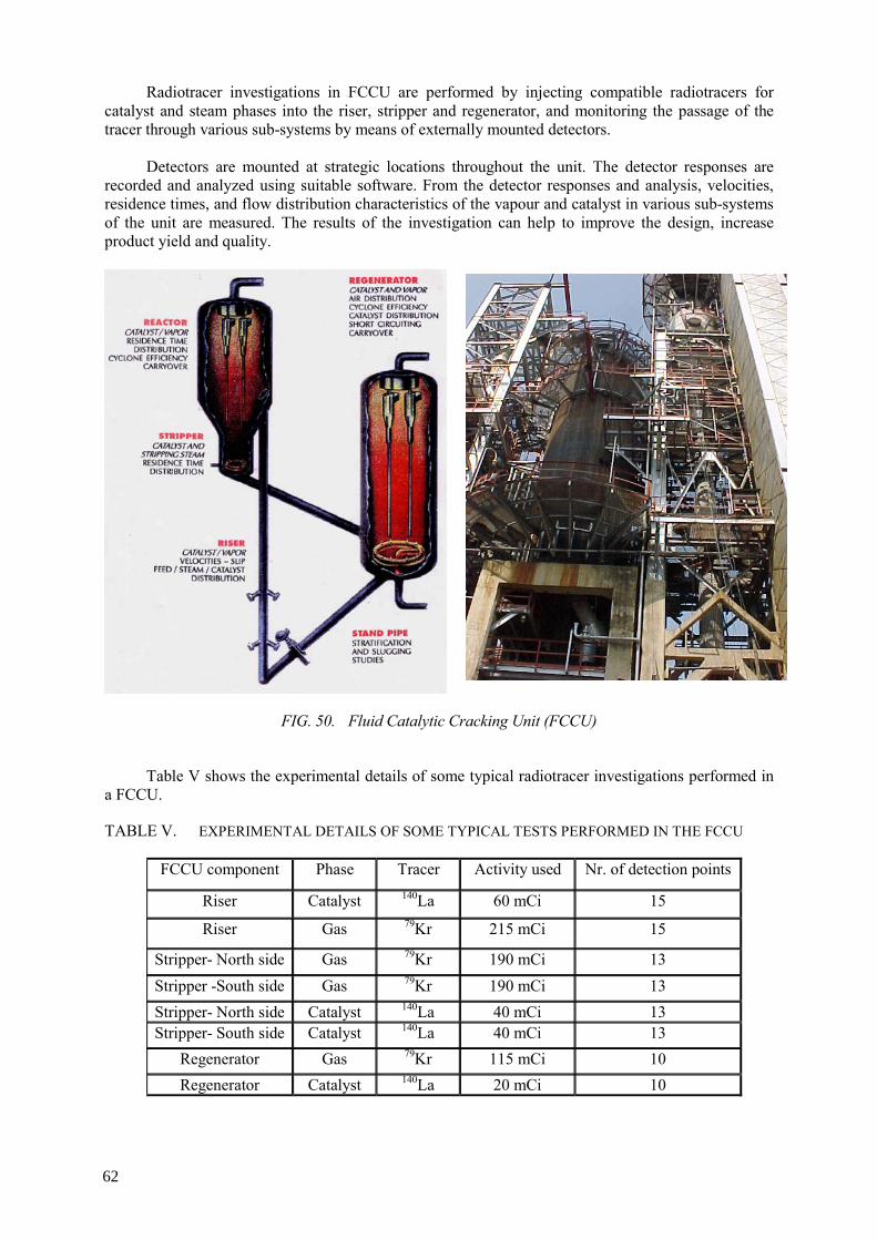
Radiotracer investigations in FCCU are performed by injecting compatible radiotracers for catalyst and steam phases into the riser, stripper and regenerator, and monitoring the passage of the tracer through various sub-systems by means of externally mounted detectors.

Detectors are mounted at strategic locations throughout the unit. The detector responses are

recorded and analyzed using suitable software. From the detector responses and analysis, velocities, residence times, and flow distribution characteristics of the vapour and catalyst in various sub-systems of the unit are measured. The results of the investigation can help to improve the design, increase product yield and quality.

FIG. 50. Fluid Catalytic Cracking Unit (FCCU)

Table V shows the experimental details of some typical radiotracer investigations performed in

a FCCU.

TABLE V. EXPERIMENTAL DETAILS OF SOME TYPICAL TESTS PERFORMED IN THE FCCU

FCCU component Phase Tracer Activity used Nr. of detection points

Riser Catalyst 140La 60 mCi 15

Riser Gas 79Kr 215 mCi 15

Stripper- North side Gas 79Kr 190 mCi 13 Stripper -South side Gas 79Kr 190 mCi 13 Stripper- North side Catalyst 140La 40 mCi 13 Stripper- South side Catalyst 140La 40 mCi 13

Regenerator Gas 79Kr 115 mCi 10 Regenerator Catalyst 140La 20 mCi 10

62

Catalyst samples are irradiated by neutrons, activating the sodium and the rare earth metals present in the catalyst. This provides a convenient tracer (La-140) to representatively follow the flow of the catalyst phase through the system. Radioactive 79Kr or 41Ar, an inert gas, can be injected to representatively follow the flow of the vapour phase through the unit.

FCCU tracer tests can provide information not easily obtained from any other source, including:

• Vapour/catalyst riser velocities and slip factors • Vapour and catalyst primary and secondary cyclone residence times • Cyclone efficiencies • Vapour and catalyst reactor residence times and mixing • Catalyst stripper and regenerator residence times • Stripper flow distribution

A. Vapour/catalyst slip factor in riser

Velocity is calculated by dividing the distance between two detectors by the elapsed time

between their responses. If this is done for both the vapour and catalyst traffic, the vapour/catalyst slip ratio can be calculated. Fig. 51 shows the results of the vapour and catalyst velocity in the riser part of the FCCU. Mean residence times of the vapour and catalyst phase were found of 1.4 and 2.3 s, respectively. Thus, the vapour and catalyst velocities were calculated of 10.5 m/s and 7.0 m/s, respectively. The slip factor resulted to be 1.5.

FIG. 51. Raiser traffic velocity and slip measurement

B. Radial distribution of vapour and catalyst flows in the riser

63

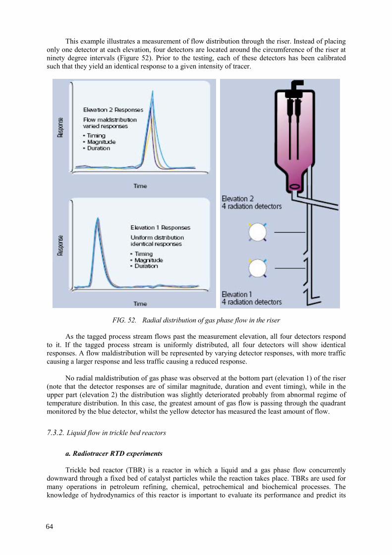
This example illustrates a measurement of flow distribution through the riser. Instead of placing only one detector at each elevation, four detectors are located around the circumference of the riser at ninety degree intervals (Figure 52). Prior to the testing, each of these detectors has been calibrated such that they yield an identical response to a given intensity of tracer.

FIG. 52. Radial distribution of gas phase flow in the riser

As the tagged process stream flows past the measurement elevation, all four detectors respond to it. If the tagged process stream is uniformly distributed, all four detectors will show identical responses. A flow maldistribution will be represented by varying detector responses, with more traffic causing a larger response and less traffic causing a reduced response.

No radial maldistribution of gas phase was observed at the bottom part (elevation 1) of the riser

(note that the detector responses are of similar magnitude, duration and event timing), while in the upper part (elevation 2) the distribution was slightly deteriorated probably from abnormal regime of temperature distribution. In this case, the greatest amount of gas flow is passing through the quadrant monitored by the blue detector, whilst the yellow detector has measured the least amount of flow.

7.3.2. Liquid flow in trickle bed reactors

a. Radiotracer RTD experiments Trickle bed reactor (TBR) is a reactor in which a liquid and a gas phase flow concurrently

downward through a fixed bed of catalyst particles while the reaction takes place. TBRs are used for many operations in petroleum refining, chemical, petrochemical and biochemical processes. The knowledge of hydrodynamics of this reactor is important to evaluate its performance and predict its

64

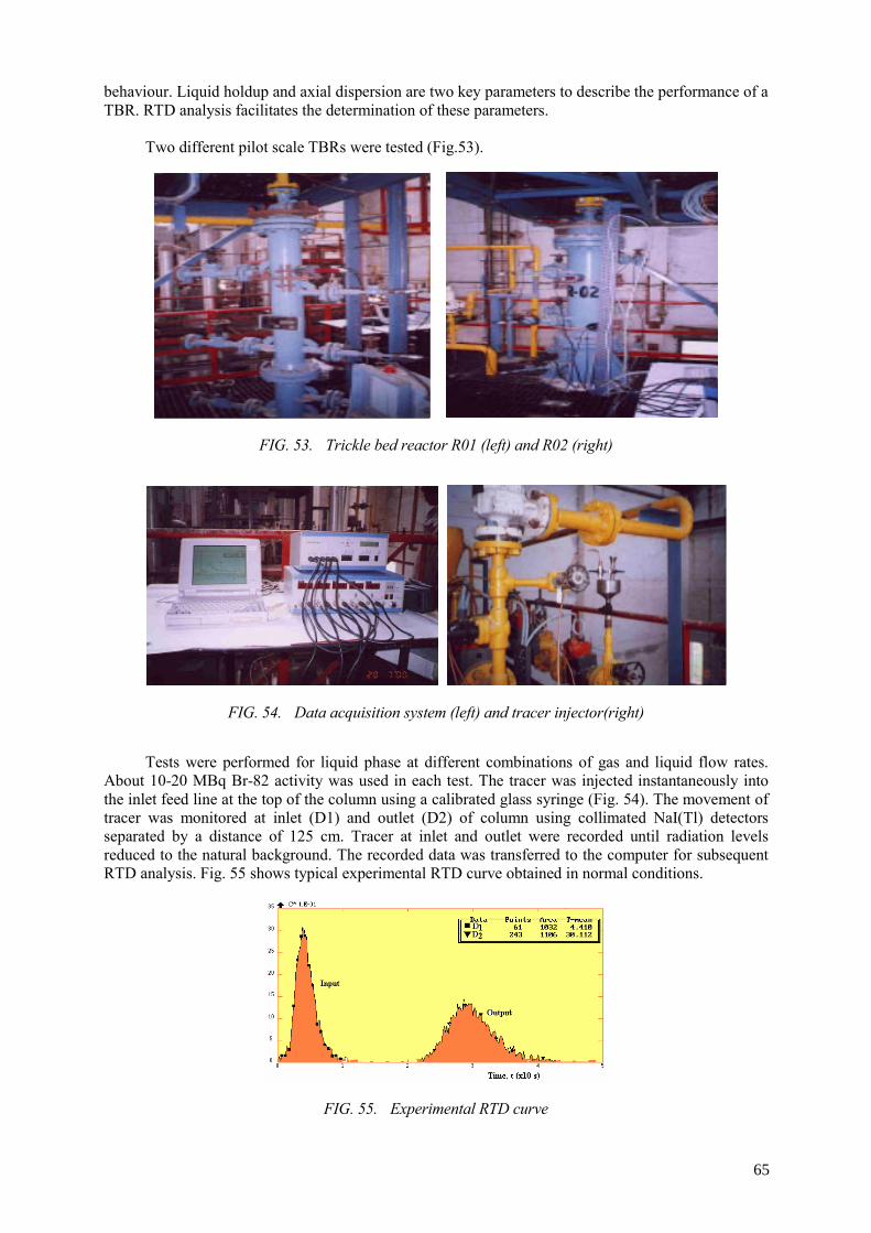
behaviour. Liquid holdup and axial dispersion are two key parameters to describe the performance of a TBR. RTD analysis facilitates the determination of these parameters.

Two different pilot scale TBRs were tested (Fig.53).

FIG. 53. Trickle bed reactor R01 (left) and R02 (right)

FIG. 54. Data acquisition system (left) and tracer injector(right)

Tests were performed for liquid phase at different combinations of gas and liquid flow rates.

About 10-20 MBq Br-82 activity was used in each test. The tracer was injected instantaneously into the inlet feed line at the top of the column using a calibrated glass syringe (Fig. 54). The movement of tracer was monitored at inlet (D1) and outlet (D2) of column using collimated NaI(Tl) detectors separated by a distance of 125 cm. Tracer at inlet and outlet were recorded until radiation levels reduced to the natural background. The recorded data was transferred to the computer for subsequent RTD analysis. Fig. 55 shows typical experimental RTD curve obtained in normal conditions.

FIG. 55. Experimental RTD curve

65

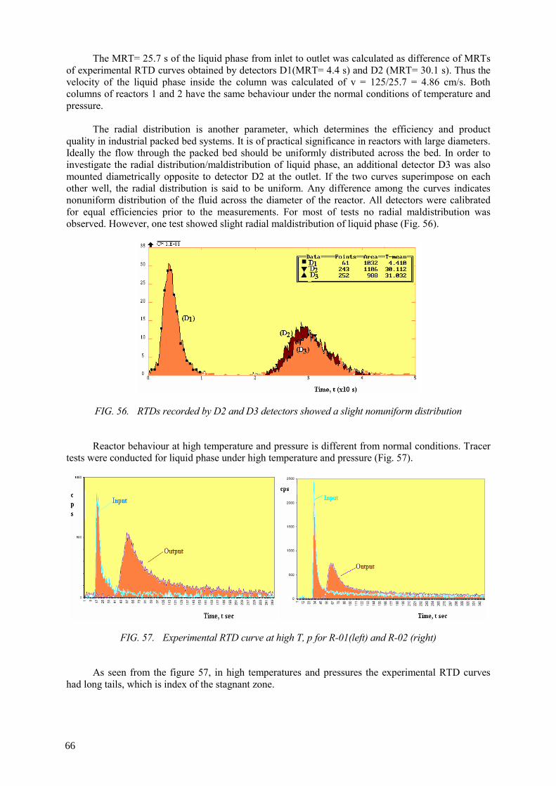
The MRT= 25.7 s of the liquid phase from inlet to outlet was calculated as difference of MRTs of experimental RTD curves obtained by detectors D1(MRT= 4.4 s) and D2 (MRT= 30.1 s). Thus the velocity of the liquid phase inside the column was calculated of v = 125/25.7 = 4.86 cm/s. Both columns of reactors 1 and 2 have the same behaviour under the normal conditions of temperature and pressure.

The radial distribution is another parameter, which determines the efficiency and product

quality in industrial packed bed systems. It is of practical significance in reactors with large diameters. Ideally the flow through the packed bed should be uniformly distributed across the bed. In order to investigate the radial distribution/maldistribution of liquid phase, an additional detector D3 was also mounted diametrically opposite to detector D2 at the outlet. If the two curves superimpose on each other well, the radial distribution is said to be uniform. Any difference among the curves indicates nonuniform distribution of the fluid across the diameter of the reactor. All detectors were calibrated for equal efficiencies prior to the measurements. For most of tests no radial maldistribution was observed. However, one test showed slight radial maldistribution of liquid phase (Fig. 56).

FIG. 56. RTDs recorded by D2 and D3 detectors showed a slight nonuniform distribution

Reactor behaviour at high temperature and pressure is different from normal conditions. Tracer

tests were conducted for liquid phase under high temperature and pressure (Fig. 57).

FIG. 57. Experimental RTD curve at high T, p for R-01(left) and R-02 (right)

As seen from the figure 57, in high temperatures and pressures the experimental RTD curves

had long tails, which is index of the stagnant zone.

66

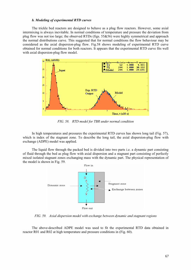
b. Modeling of experimental RTD curves The trickle bed reactors are designed to behave as a plug flow reactors. However, some axial

intermixing is always inevitable. In normal conditions of temperature and pressure the deviation from plug flow was not too large; the observed RTDs (figs. 55&56) were highly symmetrical and approach the normal distributions curve. This suggested that for normal conditions the flow behaviour may be considered as the axial dispersion-plug flow. Fig.58 shows modeling of experimental RTD curve obtained for normal conditions for both reactors. It appears that the experimental RTD curve fits well with axial dispersion-plug flow model.

FIG. 58. RTD model for TBR under normal condition

In high temperatures and pressures the experimental RTD curves has shown long tail (Fig. 57),

which is index of the stagnant zone. To describe the long tail, the axial dispersion-plug flow with exchange (ADPE) model was applied.

The liquid flow through the packed bed is divided into two parts i.e. a dynamic part consisting

of fluid through the bed as plug flow with axial dispersion and a stagnant part consisting of perfectly mixed isolated stagnant zones exchanging mass with the dynamic part. The physical representation of the model is shown in Fig. 59.

FIG. 59. Axial dispersion model with exchange between dynamic and stagnant regions

The above-described ADPE model was used to fit the experimental RTD data obtained in

reactor R01 and R02 at high temperature and pressure conditions in (Fig. 60).

67

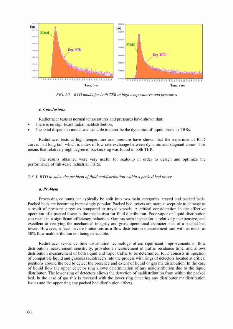
FIG. 60. RTD model for both TBR at high temperatures and pressures

c. Conclusions Radiotracer tests at normal temperatures and pressures have shown that:

• There is no significant radial maldistribution, • The axial dispersion model was suitable to describe the dynamics of liquid phase in TBRs.

Radiotracer tests at high temperature and pressure have shown that the experimental RTD curves had long tail, which is index of low rate exchange between dynamic and stagnant zones. This means that relatively high degree of backmixing was found in both TBR.

The results obtained were very useful for scale-up in order to design and optimize the

performance of full-scale industrial TBRs.

a. Problem Processing columns can typically be split into two main categories; trayed and packed beds.

Packed beds are becoming increasingly popular. Packed bed towers are more susceptible to damage as a result of pressure surges as compared to trayed vessels. A critical consideration in the effective operation of a packed tower is the mechanism for fluid distribution. Poor vapor or liquid distribution can result in a significant efficiency reduction. Gamma scan inspection is relatively inexpensive, and excellent at verifying the mechanical integrity and gross operational characteristics of a packed bed tower. However, it faces severe limitations as a flow distribution measurement tool with as much as 50% flow maldistribution not being detectable.

Radiotracer residence time distribution technology offers significant improvements in flow

distribution measurement sensitivity, provides a measurement of traffic residence time, and allows distribution measurement of both liquid and vapor traffic to be determined. RTD consists in injection of compatible liquid and gaseous radiotracers into the process with rings of detectors located at critical positions around the bed to detect the presence and extent of liquid or gas maldistribution. In the case of liquid flow the upper detector ring allows determination of any maldistribution due to the liquid distributor. The lower ring of detectors allows the detection of maldistribution from within the packed bed. In the case of gas this is reversed with the lower ring detecting any distributor maldistribution issues and the upper ring any packed bed distribution effects.

68

7.3.3. RTD to solve the problem of fluid maldistribution within a packed bed tower

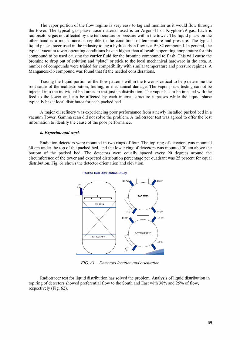
The vapor portion of the flow regime is very easy to tag and monitor as it would flow through the tower. The typical gas phase trace material used is an Argon-41 or Krypton-79 gas. Each is radioisotope gas not affected by the temperature or pressure within the tower. The liquid phase on the other hand is a much more susceptible to the conditions of temperature and pressure. The typical liquid phase tracer used in the industry to tag a hydrocarbon flow is a Br-82 compound. In general, the typical vacuum tower operating conditions have a higher than allowable operating temperature for this compound to be used causing the carrier fluid for the bromine compound to flash. This will cause the bromine to drop out of solution and “plate” or stick to the local mechanical hardware in the area. A number of compounds were trialed for compatibility with similar temperature and pressure regimes. A Manganese-56 compound was found that fit the needed considerations.

Tracing the liquid portion of the flow patterns within the tower is critical to help determine the

root cause of the maldistribution, fouling, or mechanical damage. The vapor phase testing cannot be injected into the individual bed areas to test just its distribution. The vapor has to be injected with the feed to the lower and can be affected by each internal structure it passes while the liquid phase typically has it local distributor for each packed bed.

A major oil refinery was experiencing poor performance from a newly installed packed bed in a

vacuum Tower. Gamma scan did not solve the problem. A radiotracer test was agreed to offer the best information to identify the cause of the poor performance.

b. Experimental work Radiation detectors were mounted in two rings of four. The top ring of detectors was mounted

30 cm under the top of the packed bed, and the lower ring of detectors was mounted 30 cm above the bottom of the packed bed. The detectors were equally spaced every 90 degrees around the circumference of the tower and expected distribution percentage per quadrant was 25 percent for equal distribution. Fig. 61 shows the detector orientation and elevation.

FIG. 61. Detectors location and orientation

Radiotracer test for liquid distribution has solved the problem. Analysis of liquid distribution in

top ring of detectors showed preferential flow to the South and East with 38% and 25% of flow, respectively (Fig. 62).

69

FIG. 62. Radiotracer responses of detectors at top ring

The analysis of liquid distribution in the bottom ring of detectors showed preferential flow to

the North and East quadrants with 27% and 26% of flow, respectively (Fig. 63).

FIG. 63. Radiotracer responses of detectors at lower ring

c. Conclusion Radiotracer has troubleshooted the liquid maldistribution inside the tower. Theoretically, the

liquid should behave the same in all quadrants, meaning the pulse profiles and timing should be identical for all. The data collected showed some preferential liquid flow to the South quadrant within the tower.

70

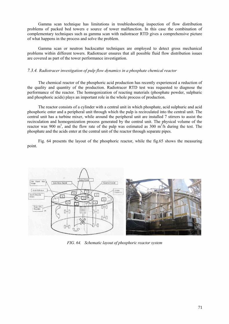
Gamma scan technique has limitations in troubleshooting inspection of flow distribution problems of packed bed towers e source of tower malfunction. In this case the combination of complementary techniques such as gamma scan with radiotracer RTD gives a comprehensive picture of what happens in the process and solve the problem.

Gamma scan or neutron backscatter techniques are employed to detect gross mechanical

problems within different towers. Radiotracer ensures that all possible fluid flow distribution issues are covered as part of the tower performance investigation.

7.3.4. Radiotracer investigation of pulp flow dynamics in a phosphate chemical reactor

The chemical reactor of the phosphoric acid production has recently experienced a reduction of

the quality and quantity of the production. Radiotracer RTD test was requested to diagnose the performance of the reactor. The homogenization of reacting materials (phosphate powder, sulphuric and phosphoric acids) plays an important role in the whole process of production.

The reactor consists of a cylinder with a central unit in which phosphate, acid sulphuric and acid

phosphoric enter and a peripheral unit through which the pulp is recirculated into the central unit. The central unit has a turbine mixer, while around the peripheral unit are installed 7 stirrers to assist the recirculation and homogenization process generated by the central unit. The physical volume of the reactor was 900 m3, and the flow rate of the pulp was estimated as 300 m3/h during the test. The phosphate and the acids enter at the central unit of the reactor through separate pipes.

Fig. 64 presents the layout of the phosphoric reactor, while the fig.65 shows the measuring

point.

FIG. 64. Schematic layout of phosphoric reactor system

71

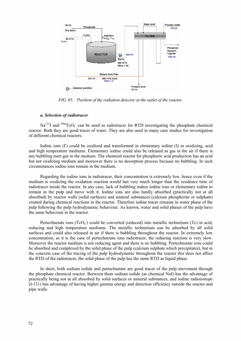
FIG. 65. Position of the radiation detector at the outlet of the reactor.

a. Selection of radiotracer Na131I and 99mTcO4

- can be used as radiotracer for RTD investigating the phosphate chemical reactor. Both they are good tracer of water. They are also used in many case studies for investigation of different chemical reactors.

Iodine ions (I-) could be oxidized and transformed in elementary iodine (I) in oxidizing, acid

and high temperature mediums. Elementary iodine could also be released as gas in the air if there is any bubbling inert gas in the medium. The chemical reactor for phosphoric acid production has an acid but not oxidizing medium and moreover there is no desorption process because no bubbling. In such circumstances iodine ions remain in the medium.

Regarding the iodine ions in radiotracer, their concentration is extremely low, hence even if the

medium is oxidizing the oxidation reaction would last very much longer than the residence time of radiotracer inside the reactor. In any case, lack of bubbling makes iodine ions or elementary iodine to remain in the pulp and move with it. Iodine ions are also hardly absorbed (practically not at all absorbed) by reactor walls (solid surfaces) and mineral substances (calcium phosphorite or sulphate) created during chemical reactions in the reactor. Therefore iodine tracer remains in water phase of the pulp following the pulp hydrodynamic behaviour. As known, water and solid phases of the pulp have the same behaviour in the reactor.

Pertechnetate ions (TcO4

-) could be converted (reduced) into metallic technetium (Tc) in acid, reducing and high temperature mediums. The metallic technetium can be adsorbed by all solid surfaces and could also released in air if there is bubbling throughout the reactor. In extremely low concentration, as it is the case of pertechnetate ions radiotracer, the reducing reaction is very slow. Moreover the reactor medium is not reducing agent and there is no bubbling. Pertechnetate ions could be absorbed and complexed by the solid phase of the pulp (calcium sulphate which precipitates), but in the concrete case of the tracing of the pulp hydrodynamic throughout the reactor this does not affect the RTD of the radiotracer; the solid phase of the pulp has the same RTD as liquid phase.

In short, both sodium iodide and pertechnetate are good tracer of the pulp movement through

the phosphate chemical reactor. Between them sodium iodide (as chemical NaI) has the advantage of practically being not at all absorbed by solid surfaces or mineral substances, and iodine radioisotope (I-131) has advantage of having higher gamma energy and detection efficiency outside the reactor and pipe walls.

72

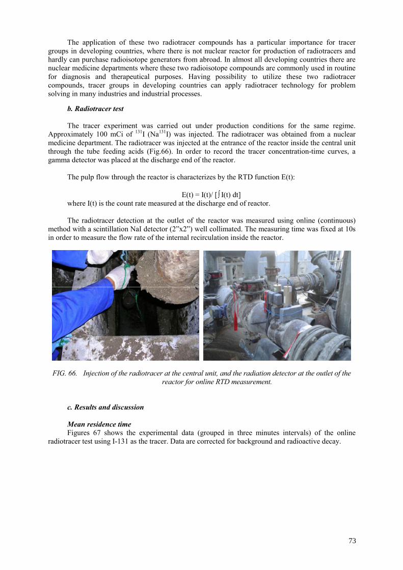
The application of these two radiotracer compounds has a particular importance for tracer groups in developing countries, where there is not nuclear reactor for production of radiotracers and hardly can purchase radioisotope generators from abroad. In almost all developing countries there are nuclear medicine departments where these two radioisotope compounds are commonly used in routine for diagnosis and therapeutical purposes. Having possibility to utilize these two radiotracer compounds, tracer groups in developing countries can apply radiotracer technology for problem solving in many industries and industrial processes.

b. Radiotracer test The tracer experiment was carried out under production conditions for the same regime.

Approximately 100 mCi of 131I (Na131I) was injected. The radiotracer was obtained from a nuclear medicine department. The radiotracer was injected at the entrance of the reactor inside the central unit through the tube feeding acids (Fig.66). In order to record the tracer concentration-time curves, a gamma detector was placed at the discharge end of the reactor.

The pulp flow through the reactor is characterizes by the RTD function E(t):

E(t) = I(t)/ [∫ I(t) dt] where I(t) is the count rate measured at the discharge end of reactor. The radiotracer detection at the outlet of the reactor was measured using online (continuous)

method with a scintillation NaI detector (2”x2”) well collimated. The measuring time was fixed at 10s in order to measure the flow rate of the internal recirculation inside the reactor.

FIG. 66. Injection of the radiotracer at the central unit, and the radiation detector at the outlet of the reactor for online RTD measurement.

c. Results and discussion Mean residence time Figures 67 shows the experimental data (grouped in three minutes intervals) of the online

radiotracer test using I-131 as the tracer. Data are corrected for background and radioactive decay.

73

FIG. 67. Experimental RTD curve (online) for I-131 tracer test and the ppercentage of the material leaving the phosphate chemical reactor each time.

The curve observed is a decaying sinusoid imposed on an exponential decay and is typical of the

response of a well-stirred system to an impulse input. There is not any long tail. Simulation of the experimental RTD curve data with a model showed that the perfect mixing

model fits better, thus the reactor was behaving almost like a perfect mixer. The mean residence time was found of MRTexp =2 h. The theoretical mean residence time calculated from physical volume V =900 m3 and flow rate Q = 300 m3/h was calculated of MRTth = 3 h.

Based on the experimental MRT the active volume of the reactor during the experimental time

was calculated of: Va = Q x MRTexp = 300 m3/h x 2h = 600 m3

The non-active volume is consequently estimated of nearly 300 m3. This means that nearly 1/3

of the reactor volume is inactive to the process. Based of the regular form of the RTD curve (without any long tail) it can be stated that the inactive volume in this case is very probably a dead volume or a blocked volume by the solidified material (slag). The perfect mixing model indicates that parts of the pulp are staying inside the reactor from few seconds till nearly 6 hours. This is shown from the cumulative RTD function F(t) = Σ E(t) Δt (Fig. 68). The cumulative curve can be useful when analyzing the behaviour of the reactor. The distribution of the contact times results relatively large: there are raw materials leaving the reactor very early without undertaking the chemical reaction (reducing the quality of production), as well as there is pulp remaining in the reactor much longer that needed, spending energy and reducing the yield. Fig. 67 shows that 20% of the material leaves the reactor in nearly 0.5 h; 30 % of the material goes out the reactor in less than 1 h, 60% of the material exits in less than 2 h; 80% goes in around 3 h and 90% needs only 4 h to go out.

Estimation of the flow rate of the internal recirculation. Recycles in principle should be indicated in the experimental RTD curves by peaks accepting

the assumption that every recycle gives a maximum of the record in the outlet of the reactor. A recycle is counted from the moment the pulp enters the central unit, moving throughout the central unit vortex, leaving it in overflow, and circulating the peripheral unit in unique sense until arriving again to the central unit from its bottom part. In front of this turning point is located the output pipe. The recycled pulp is splitting in two parts, one part leaving the reactor and the other part continuing the next recycle.

74

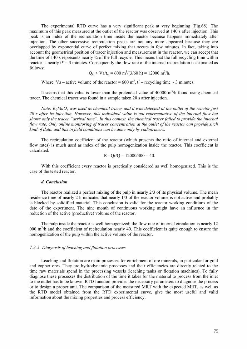
The experimental RTD curve has a very significant peak at very beginning (Fig.68). The maximum of this peak measured at the outlet of the reactor was observed at 140 s after injection. This peak is an index of the recirculation time inside the reactor because happens immediately after injection. The other successive recirculation peaks are not any more appeared because they are overlapped by exponential curve of perfect mixing that occurs in few minutes. In fact, taking into account the geometrical position of tracer injection and measurement in the reactor, we can accept that the time of 140 s represents nearly ¾ of the full recycle. This means that the full recycling time within reactor is nearly t* = 3 minutes. Consequently the flow rate of the internal recirculation is estimated as follows:

Qin > Va/tm = 600 m3/(3/60 h) = 12000 m3/h. Where: Va – active volume of the reactor = 600 m3, t* – recycling time ~ 3 minutes. It seems that this value is lower than the pretended value of 40000 m3/h found using chemical

tracer. The chemical tracer was found in a sample taken 20 s after injection. Note: K2MnO4 was used as chemical tracer and it was detected at the outlet of the reactor just

20 s after its injection. However, this individual value is not representative of the internal flow but shows only the tracer “arrival time”. In this context, the chemical tracer failed to provide the internal flow rate. Only online monitoring of tracer concentration at the outlet of the reactor can provide such kind of data, and this in field conditions can be done only by radiotracers.

The recirculation coefficient of the reactor (which presents the ratio of internal and external

flow rates) is much used as index of the pulp homogenization inside the reactor. This coefficient is calculated:

R= Qr/Q = 12000/300 = 40. With this coefficient every reactor is practically considered as well homogenized. This is the

case of the tested reactor. d. Conclusion The reactor realized a perfect mixing of the pulp in nearly 2/3 of its physical volume. The mean

residence time of nearly 2 h indicates that nearly 1/3 of the reactor volume is not active and probably is blocked by solidified material. This conclusion is valid for the reactor working conditions of the date of the experiment. The nine month of continuous working might have an influence in the reduction of the active (productive) volume of the reactor.

The pulp inside the reactor is well homogenized; the flow rate of internal circulation is nearly 12

000 m3/h and the coefficient of recirculation nearly 40. This coefficient is quite enough to ensure the homogenization of the pulp within the active volume of the reactor.

7.3.5. Diagnosis of leaching and flotation processes

Leaching and flotation are main processes for enrichment of ore minerals, in particular for gold

and copper ores. They are hydrodynamic processes and their efficiencies are directly related to the time raw materials spend in the processing vessels (leaching tanks or flotation machines). To fully diagnose these processes the distribution of the time it takes for the material to process from the inlet to the outlet has to be known. RTD function provides the necessary parameters to diagnose the process or to design a proper unit. The comparison of the measured MRT with the expected MRT, as well as the RTD model obtained from the RTD experimental curve, give the most useful and valid information about the mixing properties and process efficiency.

75

A. Diagnosis of gold slurry leaching tanks RTD method was applied in a gold enrichment plant. The most important part of the gold

processing plant is the leaching process, which is being carried out in eight processing tanks of the leaching line (Fig.68). The gold slurry (after grinding process) is overflowing from cyclone to the first tank and after it is going through all tanks where gold ore leaching taken place. The overall flow rate through tanks was 100 m3/h.

Taking into account the importance of the leaching process in final gold recovery the RTD

method was applied to diagnose the process functioning throughout the processing tanks. The main objectives of the radiotracer investigation were:

• to measure the slurry retention time of tanks 1 (volume 500 m3), 7 and 8 (volume 250 m3 each

one), as the most important tanks in leaching process, • to judge about macromixing of slurry within these tanks, • to locate possible malfunctions inside the processing tanks.

Potassium bromide K82Br liquid radiotracer was used to investigate the leaching tanks in the

plant. The radiotracer was prepared at the nuclear reactor. The activity of radiotracer injected in the tank 1 was 100 mCi at the injection time, while the activity of radiotracer injected to the inlet of tank 7 to diagnose both tanks 7 and 8 was 130 mCi.

FIG. 68. Tracer experiment in gold leaching tanks

FIG. 69. Taking samples (left) and measuring them with Marineli can on top of NaI detector (left)

76

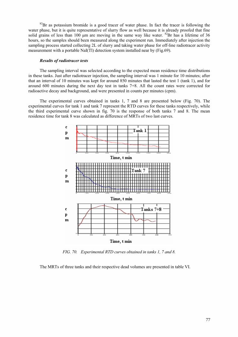
82Br as potassium bromide is a good tracer of water phase. In fact the tracer is following the water phase, but it is quite representative of slurry flow as well because it is already proofed that fine solid grains of less than 100 μm are moving in the same way like water. 82Br has a lifetime of 36 hours, so the samples should been measured along the experiment run. Immediately after injection the sampling process started collecting 2L of slurry and taking water phase for off-line radiotracer activity measurement with a portable NaI(Tl) detection system installed near by (Fig.69).

Results of radiotracer tests The sampling interval was selected according to the expected mean residence time distributions

in these tanks. Just after radiotracer injection, the sampling interval was 1 minute for 10 minutes; after that an interval of 10 minutes was kept for around 850 minutes that lasted the test 1 (tank 1), and for around 600 minutes during the next day test in tanks 7+8. All the count rates were corrected for radioactive decay and background, and were presented in counts per minutes (cpm).

The experimental curves obtained in tanks 1, 7 and 8 are presented below (Fig. 70). The

experimental curves for tank 1 and tank 7 represent the RTD curves for these tanks respectively, while the third experimental curve shown in fig. 70 is the response of both tanks 7 and 8. The mean residence time for tank 8 was calculated as difference of MRTs of two last curves.

FIG. 70. Experimental RTD curves obtained in tanks 1, 7 and 8.

The MRTs of three tanks and their respective dead volumes are presented in table VI.

77

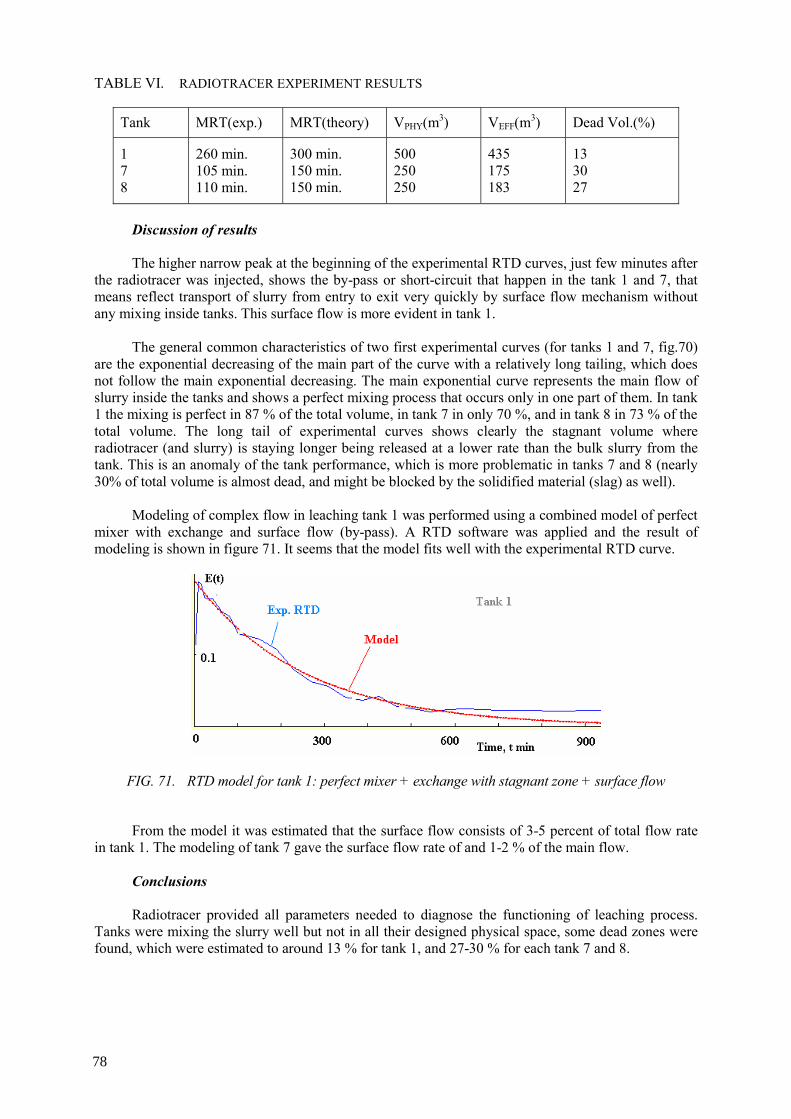
TABLE VI. RADIOTRACER EXPERIMENT RESULTS

Tank MRT(exp.) MRT(theory) VPHY(m3) VEFF(m3) Dead Vol.(%)

1 7 8

260 min. 105 min. 110 min.

300 min. 150 min. 150 min.

500 250 250

435 175 183

13 30 27

Discussion of results The higher narrow peak at the beginning of the experimental RTD curves, just few minutes after

the radiotracer was injected, shows the by-pass or short-circuit that happen in the tank 1 and 7, that means reflect transport of slurry from entry to exit very quickly by surface flow mechanism without any mixing inside tanks. This surface flow is more evident in tank 1.

The general common characteristics of two first experimental curves (for tanks 1 and 7, fig.70)

are the exponential decreasing of the main part of the curve with a relatively long tailing, which does not follow the main exponential decreasing. The main exponential curve represents the main flow of slurry inside the tanks and shows a perfect mixing process that occurs only in one part of them. In tank 1 the mixing is perfect in 87 % of the total volume, in tank 7 in only 70 %, and in tank 8 in 73 % of the total volume. The long tail of experimental curves shows clearly the stagnant volume where radiotracer (and slurry) is staying longer being released at a lower rate than the bulk slurry from the tank. This is an anomaly of the tank performance, which is more problematic in tanks 7 and 8 (nearly 30% of total volume is almost dead, and might be blocked by the solidified material (slag) as well).

Modeling of complex flow in leaching tank 1 was performed using a combined model of perfect

mixer with exchange and surface flow (by-pass). A RTD software was applied and the result of modeling is shown in figure 71. It seems that the model fits well with the experimental RTD curve.

FIG. 71. RTD model for tank 1: perfect mixer + exchange with stagnant zone + surface flow

From the model it was estimated that the surface flow consists of 3-5 percent of total flow rate

in tank 1. The modeling of tank 7 gave the surface flow rate of and 1-2 % of the main flow. Conclusions Radiotracer provided all parameters needed to diagnose the functioning of leaching process.

Tanks were mixing the slurry well but not in all their designed physical space, some dead zones were found, which were estimated to around 13 % for tank 1, and 27-30 % for each tank 7 and 8.

78

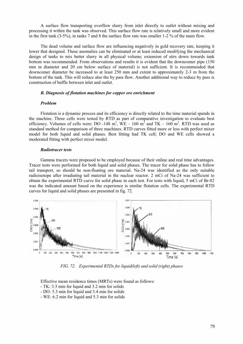
A surface flow transporting overflow slurry from inlet directly to outlet without mixing and processing it within the tank was observed. This surface flow rate is relatively small and more evident in the first tank (3-5%), in tanks 7 and 8 the surface flow rate was smaller 1-2 % of the main flow.

The dead volume and surface flow are influencing negatively in gold recovery rate, keeping it

lower that designed. These anomalies can be eliminated or at least reduced modifying the mechanical design of tanks to mix better slurry in all physical volume; extension of stirs down towards tank bottom was recommended. From observations and results it is evident that the downcomer pipe (150 mm in diameter and 20 cm below surface of material) is not sufficient. It is recommended that downcomer diameter be increased to at least 250 mm and extent to approximately 2-3 m from the bottom of the tank. This will reduce also the by pass flow. Another additional way to reduce by pass is construction of baffle between inlet and outlet.

B. Diagnosis of flotation machines for copper ore enrichment Problem Flotation is a dynamic process and its efficiency is directly related to the time material spends in

the machine. Three cells were tested by RTD as part of comparative investigation to evaluate best efficiency. Volumes of cells were: DO -148 m3, WE – 160 m3 and TK – 160 m3. RTD was used as standard method for comparison of three machines. RTD curves fitted more or less with perfect mixer model for both liquid and solid phases. Best fitting had TK cell; DO and WE cells showed a moderated fitting with perfect mixer model.

Radiotracer tests Gamma tracers were proposed to be employed because of their online and real time advantages.

Tracer tests were performed for both liquid and solid phases. The tracer for solid phase has to follow tail transport, so should be non-floating ore material. Na-24 was identified as the only suitable radioisotope after irradiating tail material in the nuclear reactor. 2 mCi of Na-24 was sufficient to obtain the experimental RTD curve for solid phase in each test. For tests with liquid, 5 mCi of Br-82 was the indicated amount based on the experience is similar flotation cells. The experimental RTD curves for liquid and solid phases are presented in fig. 72.

FIG. 72. Experimental RTDs for liquid(left) and solid (right) phases

Effective mean residence times (MRTs) were found as follows: - TK: 3.3 min for liquid and 3.2 min for solids - DO: 5.3 min for liquid and 3.4 min for solids - WE: 6.2 min for liquid and 5.3 min for solids

79

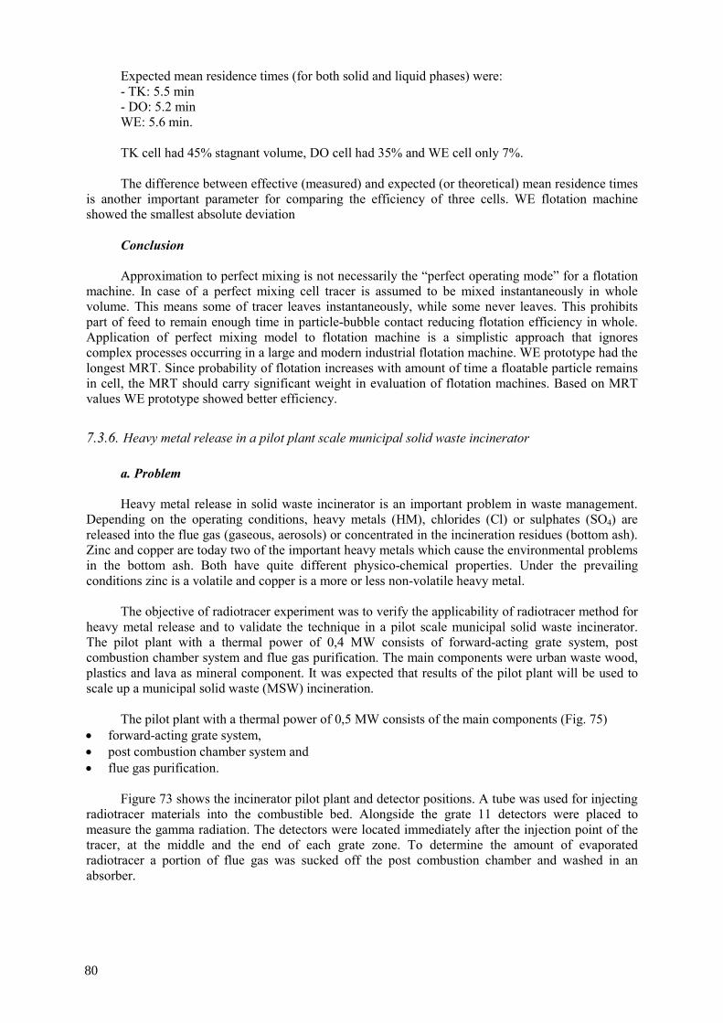
Expected mean residence times (for both solid and liquid phases) were: - TK: 5.5 min - DO: 5.2 min WE: 5.6 min. TK cell had 45% stagnant volume, DO cell had 35% and WE cell only 7%. The difference between effective (measured) and expected (or theoretical) mean residence times

is another important parameter for comparing the efficiency of three cells. WE flotation machine showed the smallest absolute deviation

Conclusion Approximation to perfect mixing is not necessarily the “perfect operating mode” for a flotation

machine. In case of a perfect mixing cell tracer is assumed to be mixed instantaneously in whole volume. This means some of tracer leaves instantaneously, while some never leaves. This prohibits part of feed to remain enough time in particle-bubble contact reducing flotation efficiency in whole. Application of perfect mixing model to flotation machine is a simplistic approach that ignores complex processes occurring in a large and modern industrial flotation machine. WE prototype had the longest MRT. Since probability of flotation increases with amount of time a floatable particle remains in cell, the MRT should carry significant weight in evaluation of flotation machines. Based on MRT values WE prototype showed better efficiency.

7.3.6. Heavy metal release in a pilot plant scale municipal solid waste incinerator a. Problem Heavy metal release in solid waste incinerator is an important problem in waste management.

Depending on the operating conditions, heavy metals (HM), chlorides (Cl) or sulphates (SO4) are released into the flue gas (gaseous, aerosols) or concentrated in the incineration residues (bottom ash). Zinc and copper are today two of the important heavy metals which cause the environmental problems in the bottom ash. Both have quite different physico-chemical properties. Under the prevailing conditions zinc is a volatile and copper is a more or less non-volatile heavy metal.

The objective of radiotracer experiment was to verify the applicability of radiotracer method for

heavy metal release and to validate the technique in a pilot scale municipal solid waste incinerator. The pilot plant with a thermal power of 0,4 MW consists of forward-acting grate system, post combustion chamber system and flue gas purification. The main components were urban waste wood, plastics and lava as mineral component. It was expected that results of the pilot plant will be used to scale up a municipal solid waste (MSW) incineration.

• forward-acting grate system, • post combustion chamber system and • flue gas purification.

Figure 73 shows the incinerator pilot plant and detector positions. A tube was used for injecting

radiotracer materials into the combustible bed. Alongside the grate 11 detectors were placed to measure the gamma radiation. The detectors were located immediately after the injection point of the tracer, at the middle and the end of each grate zone. To determine the amount of evaporated radiotracer a portion of flue gas was sucked off the post combustion chamber and washed in an absorber.

80

The pilot plant with a thermal power of 0,5 MW consists of the main components (Fig. 75)

FIG. 73. Incinerator pilot plant and detector positions

b. Radiotracer experiments The radiotracer must fulfill following requirements:

• heavy metal isotopes with the same chemical properties as the inactive heavy metals • emitters of gamma rays for on-line measurements through relatively thick reactor walls, • short radioactive half-life (some hours until a few days) for radiation safety consideration.

The radioisotopes 64Cu and 69mZn meet these requirements and were used as radiotracers. The

isotope 64Cu has a half-life of 12.7 hours and emits gamma rays with energy of 511 keV with a probability of 37 % due to positron annihilation. The isotope 69mZn has a half-life of 13.8 hours and emits gamma rays with energy of 439 keV. Both isotopes were produced in a research reactor by neutron activation. For preparation of 64Cu a pure copper metal was irradiated, while for 69mZn highly enriched target of 68Zn was manufactured and irradiated into the nuclear reactor.

For each experiment 200 mCi of 64Cu and of 69mZn, respectively, were used. The ampoule was

cracked; its content was mixed with 20 grams of waste material and pressed into a pellet. This single pellet was injected instantaneously (Dirac pulse) at the entry of the grate through an injection tube. 1” NaI(Tl) scintillation detectors, collimated with tungsten alloy, were used to measure the radiotracer. The mean residence time distributions of the solid phase movement inside the incinerator was determined injecting 113mIn2O3 (200 mCi), which is an inert tracer to this process.

For determination of the quantity of copper and zinc in the flue gas an absorber filled with

diluted nitric acid was used. A partial flow of the flue gas was continuously punched from the combustion chamber and passed through the absorber. An unshielded 1.5” NaI(Tl) scintillation detector positioned in the centre of the absorber recorded the absorbed quantity of radioactive metal as a function of time. At the end of each experimental run the dissolved content of an irradiated ampoule containing the small quantity of the corresponding metal was given directly into the absorber for calibration.

81

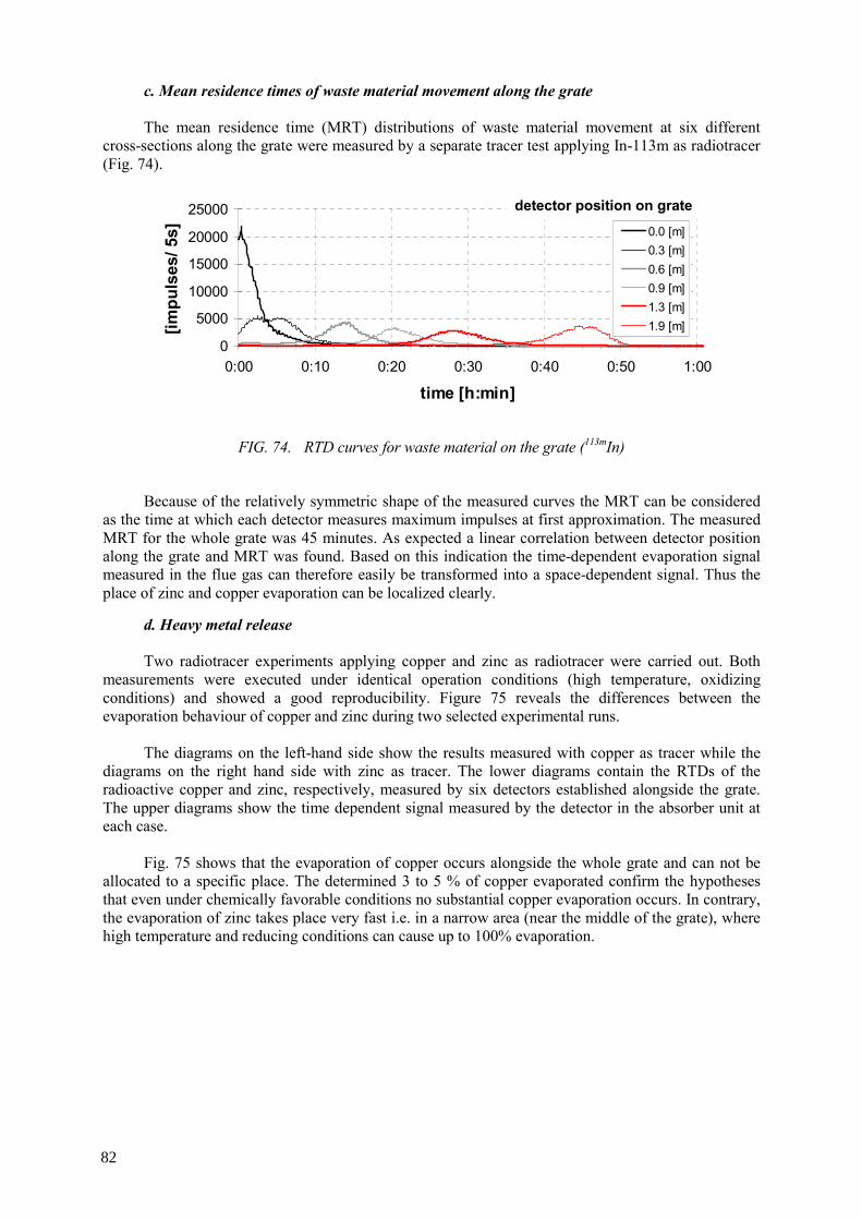
c. Mean residence times of waste material movement along the grate The mean residence time (MRT) distributions of waste material movement at six different

cross-sections along the grate were measured by a separate tracer test applying In-113m as radiotracer (Fig. 74).

0

5000

10000

15000

20000

25000

0:00 0:10 0:20 0:30 0:40 0:50 1:00

time [h:min]

[impu

lses

/ 5s] 0.0 [m]

0.3 [m]0.6 [m]0.9 [m]1.3 [m]1.9 [m]

detector position on grate

FIG. 74. RTD curves for waste material on the grate (113mIn)

Because of the relatively symmetric shape of the measured curves the MRT can be considered

as the time at which each detector measures maximum impulses at first approximation. The measured MRT for the whole grate was 45 minutes. As expected a linear correlation between detector position along the grate and MRT was found. Based on this indication the time-dependent evaporation signal measured in the flue gas can therefore easily be transformed into a space-dependent signal. Thus the place of zinc and copper evaporation can be localized clearly.

d. Heavy metal release Two radiotracer experiments applying copper and zinc as radiotracer were carried out. Both

measurements were executed under identical operation conditions (high temperature, oxidizing conditions) and showed a good reproducibility. Figure 75 reveals the differences between the evaporation behaviour of copper and zinc during two selected experimental runs.

The diagrams on the left-hand side show the results measured with copper as tracer while the

diagrams on the right hand side with zinc as tracer. The lower diagrams contain the RTDs of the radioactive copper and zinc, respectively, measured by six detectors established alongside the grate. The upper diagrams show the time dependent signal measured by the detector in the absorber unit at each case.

Fig. 75 shows that the evaporation of copper occurs alongside the whole grate and can not be

allocated to a specific place. The determined 3 to 5 % of copper evaporated confirm the hypotheses that even under chemically favorable conditions no substantial copper evaporation occurs. In contrary, the evaporation of zinc takes place very fast i.e. in a narrow area (near the middle of the grate), where high temperature and reducing conditions can cause up to 100% evaporation.

82

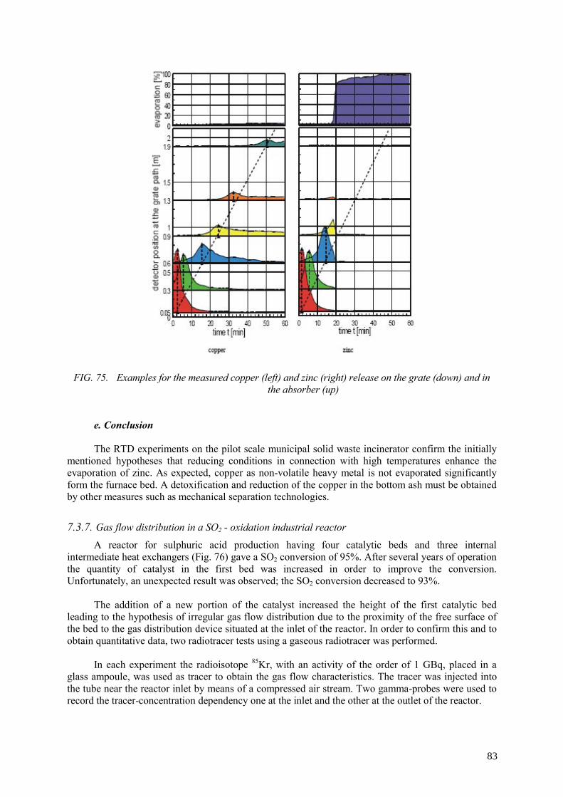
FIG. 75. Examples for the measured copper (left) and zinc (right) release on the grate (down) and in the absorber (up)

e. Conclusion The RTD experiments on the pilot scale municipal solid waste incinerator confirm the initially

mentioned hypotheses that reducing conditions in connection with high temperatures enhance the evaporation of zinc. As expected, copper as non-volatile heavy metal is not evaporated significantly form the furnace bed. A detoxification and reduction of the copper in the bottom ash must be obtained by other measures such as mechanical separation technologies.

7.3.7. Gas flow distribution in a SO2 - oxidation industrial reactor

A reactor for sulphuric acid production having four catalytic beds and three internal intermediate heat exchangers (Fig. 76) gave a SO2 conversion of 95%. After several years of operation the quantity of catalyst in the first bed was increased in order to improve the conversion. Unfortunately, an unexpected result was observed; the SO2 conversion decreased to 93%.

The addition of a new portion of the catalyst increased the height of the first catalytic bed leading to the hypothesis of irregular gas flow distribution due to the proximity of the free surface of the bed to the gas distribution device situated at the inlet of the reactor. In order to confirm this and to obtain quantitative data, two radiotracer tests using a gaseous radiotracer was performed.

In each experiment the radioisotope 85Kr, with an activity of the order of 1 GBq, placed in a

glass ampoule, was used as tracer to obtain the gas flow characteristics. The tracer was injected into the tube near the reactor inlet by means of a compressed air stream. Two gamma-probes were used to record the tracer-concentration dependency one at the inlet and the other at the outlet of the reactor.

83

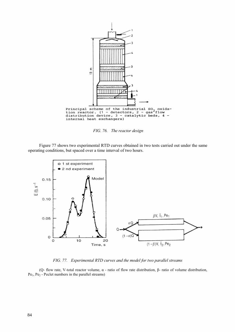
FIG. 76.

Figure 77 shows two experimental RTD curves obtained in two tests carried out under the same

operating conditions, but spaced over a time interval of two hours.

FIG. 77. Experimental RTD curves and the model for two parallel streams

(Q- flow rate, V-total reactor volume, α - ratio of flow rate distribution, β- ratio of volume distribution, Pe1, Pe2 - Peclet numbers in the parallel streams)

84

The reactor design

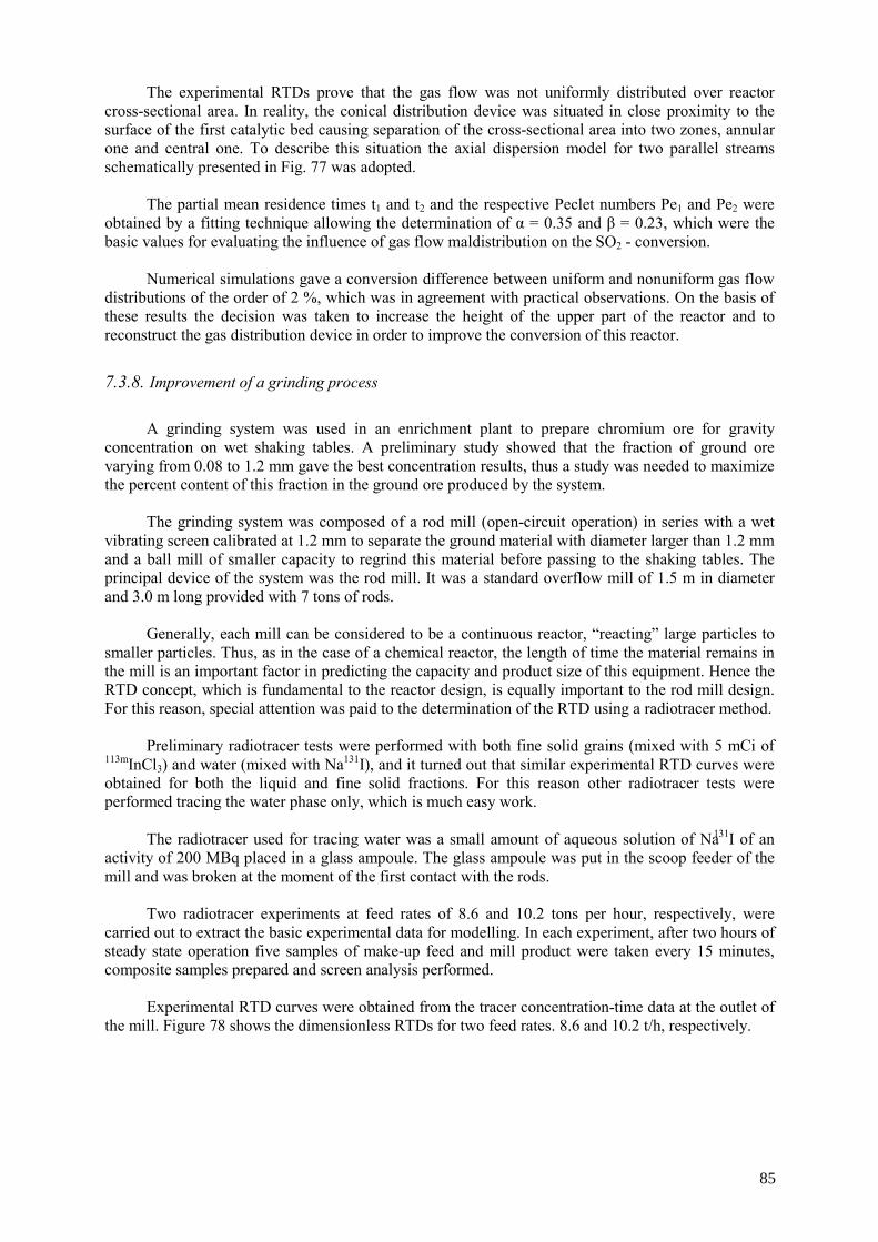
The experimental RTDs prove that the gas flow was not uniformly distributed over reactor cross-sectional area. In reality, the conical distribution device was situated in close proximity to the surface of the first catalytic bed causing separation of the cross-sectional area into two zones, annular one and central one. To describe this situation the axial dispersion model for two parallel streams schematically presented in Fig. 77 was adopted.

The partial mean residence times t1 and t2 and the respective Peclet numbers Pe1 and Pe2 were

obtained by a fitting technique allowing the determination of α = 0.35 and β = 0.23, which were the basic values for evaluating the influence of gas flow maldistribution on the SO2 - conversion.

Numerical simulations gave a conversion difference between uniform and nonuniform gas flow

distributions of the order of 2 %, which was in agreement with practical observations. On the basis of these results the decision was taken to increase the height of the upper part of the reactor and to reconstruct the gas distribution device in order to improve the conversion of this reactor.

7.3.8. Improvement of a grinding process

A grinding system was used in an enrichment plant to prepare chromium ore for gravity

concentration on wet shaking tables. A preliminary study showed that the fraction of ground ore varying from 0.08 to 1.2 mm gave the best concentration results, thus a study was needed to maximize the percent content of this fraction in the ground ore produced by the system.

The grinding system was composed of a rod mill (open-circuit operation) in series with a wet

vibrating screen calibrated at 1.2 mm to separate the ground material with diameter larger than 1.2 mm and a ball mill of smaller capacity to regrind this material before passing to the shaking tables. The principal device of the system was the rod mill. It was a standard overflow mill of 1.5 m in diameter and 3.0 m long provided with 7 tons of rods.

Generally, each mill can be considered to be a continuous reactor, “reacting” large particles to

smaller particles. Thus, as in the case of a chemical reactor, the length of time the material remains in the mill is an important factor in predicting the capacity and product size of this equipment. Hence the RTD concept, which is fundamental to the reactor design, is equally important to the rod mill design. For this reason, special attention was paid to the determination of the RTD using a radiotracer method.

Preliminary radiotracer tests were performed with both fine solid grains (mixed with 5 mCi of

113mInCl3) and water (mixed with Na131I), and it turned out that similar experimental RTD curves were obtained for both the liquid and fine solid fractions. For this reason other radiotracer tests were performed tracing the water phase only, which is much easy work.

131I of an

activity of 200 MBq placed in a glass ampoule. The glass ampoule was put in the scoop feeder of the mill and was broken at the moment of the first contact with the rods.

Two radiotracer experiments at feed rates of 8.6 and 10.2 tons per hour, respectively, were

carried out to extract the basic experimental data for modelling. In each experiment, after two hours of steady state operation five samples of make-up feed and mill product were taken every 15 minutes, composite samples prepared and screen analysis performed.

Experimental RTD curves were obtained from the tracer concentration-time data at the outlet of the mill. Figure 78 shows the dimensionless RTDs for two feed rates. 8.6 and 10.2 t/h, respectively.

85

The radiotracer used for tracing water was a small amount of aqueous solution of Na

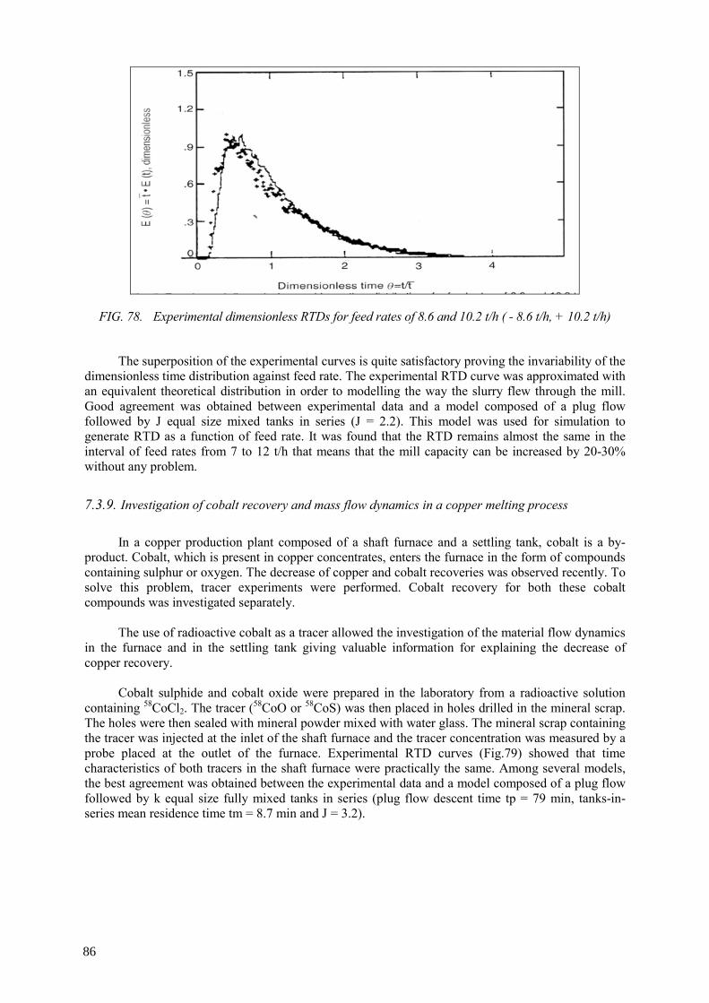
FIG. 78. Experimental dimensionless RTDs for feed rates of 8.6 and 10.2 t/h ( - 8.6 t/h, + 10.2 t/h)

The superposition of the experimental curves is quite satisfactory proving the invariability of the

dimensionless time distribution against feed rate. The experimental RTD curve was approximated with an equivalent theoretical distribution in order to modelling the way the slurry flew through the mill. Good agreement was obtained between experimental data and a model composed of a plug flow followed by J equal size mixed tanks in series (J = 2.2). This model was used for simulation to generate RTD as a function of feed rate. It was found that the RTD remains almost the same in the interval of feed rates from 7 to 12 t/h that means that the mill capacity can be increased by 20-30% without any problem.

7.3.9. Investigation of cobalt recovery and mass flow dynamics in a copper melting process

In a copper production plant composed of a shaft furnace and a settling tank, cobalt is a by-

product. Cobalt, which is present in copper concentrates, enters the furnace in the form of compounds containing sulphur or oxygen. The decrease of copper and cobalt recoveries was observed recently. To solve this problem, tracer experiments were performed. Cobalt recovery for both these cobalt compounds was investigated separately.

The use of radioactive cobalt as a tracer allowed the investigation of the material flow dynamics

in the furnace and in the settling tank giving valuable information for explaining the decrease of copper recovery.

Cobalt sulphide and cobalt oxide were prepared in the laboratory from a radioactive solution

containing 58CoCl2. The tracer (58CoO or 58CoS) was then placed in holes drilled in the mineral scrap. The holes were then sealed with mineral powder mixed with water glass. The mineral scrap containing the tracer was injected at the inlet of the shaft furnace and the tracer concentration was measured by a probe placed at the outlet of the furnace. Experimental RTD curves (Fig.79) showed that time characteristics of both tracers in the shaft furnace were practically the same. Among several models, the best agreement was obtained between the experimental data and a model composed of a plug flow followed by k equal size fully mixed tanks in series (plug flow descent time tp = 79 min, tanks-in-series mean residence time tm = 8.7 min and J = 3.2).

86

FIG. 79. Experimental RTDs of 58Co0 and 58CoS at the outlet of the shaft furnace (1 – 58CoO, 2 - 58CoS, 3 – model k=3.2)

Thus, the RTD in the shaft fu4rnace indicated a plug flow corresponding to descent movement of the solid material coupled with appreciable mixing corresponding to the movement of the material in the melting zone. The ratio of characteristic times given above showed that the melted mass occupied about 10% of the total mass in the furnace.

After the tracer had passed from the furnace into the settling tank, sampling of both waste slag

and copper-matte was carried out for a period of about six hours and the sample measurements were performed using a lead-shielded NaI (TI) detector coupled to a single-channel analyzer. Sampling technique was necessary in settling tank for tracer balance and RTD measurement. The tracer balance in the copper-matte and in the waste slag revealed that values from 70 to 75% may be considered the most probable for cobalt recovery in the copper-matte, regardless of the nature of the original chemical compound in the raw material.

Figure 80 represents the normalized RTD curves at the outlet of the settling tank. The two

tracers gave almost the same RTD showing that the behaviour of cobalt in the settling tank was (like in the furnace) independent of its original chemical form.

FIG. 80. Normalized tracer concentration distributions at the outlet of the settling tank (1 - 58CoO, 2 - 58CoS, 3 - model)

87

The experimental RTDs indicated the existence of a lag and a short circuit. It was tried to describe these phenomena by a time-delay model which had been applied for the description of the movement of high viscosity liquids and molten plastics. The free parameter of this model was the mean delay time td, from which the percentage of flow in the short circuit can be calculated.

A good agreement between the theoretical curve and the experimental data was obtained for td =

40 min giving a percentage of short circuit of the order of 5%. This short circuit can explain the decrease in copper recovery. From the experimental RTD and its model it was also estimated that nearly 30% of the volume of the settling tank was blocked by the solidified material. The decrease in the active volume may be one of the reasons for the short circuit, the other, not less important, may be the geometrical form of the settling tank. In order to eliminate the short circuit recommendations were provided to plant engineers to stop the shaft furnace, to discharge the settling tank and to consider the possibility of its reconstruction according to a better design.

7.3.10. Estimation of laterite grain erosion in a fluidised bed calciner

Nickel is extracted by treatment of laterites with ammonia. A fluidized bed calciner was used to

alter the internal structure of a ground laterite mineral before treatment with a reducing gas mixture (CO+H2). The granulometric composition of the iron mineral ore entering the calciner was ranged from 0 to 6 mm, with 60% of material between 150 μm and 1 mm. The operation of the calciner over several years was accompanied by the production of large amounts of dust (0-100 μm), which was carried by the current of the reducing gas overloading and frequently blocking the cleaning system. The dust released to the air from the chimney (0-100 μm) sometimes increased up to 25-30 % of the entry mass, when the natural dust part of the ground laterite mineral entering the calciner was nearly 10 % only. It was thought that a considerable part of the dust was formed in the calciner due to erosion of mineral particles. Thus, a series of experiments with radiotracers was performed in order to confirm this hypothesis and to obtain quantitative data.

Several mineral fractions of different diameter were selected and activated in a nuclear reactor

to produce the 59Fe. In each experiment, 100 g of the mineral labelled with a total activity of 800 MBq of 59Fe was encapsulated into polyethylene bags and placed on the conveyor which carried the mineral into the calciner. Scintillation gamma detectors were placed at the outlets of dusty gas and of calcined mineral to record the tracer concentrations against time. From experimental data the mean residence time tm and the eroded portion for each fraction F(D0) against its initial diameter D0 were obtained. These results are presented in Figs. 81 and 82, respectively.

FIG. 81. Mean residence times of ground mineral fractions in the fluidized bed as a function of their initial mean diameter (o – experiment, _model)

88

FIG. 82. Portion of the fraction which is broken up by erosion in relation to its initial mean diameter (o - experiment, __model)

The portion of the fraction which is destroyed by erosion depends on two factors: the specific

surface and the mean residence time. With an increase in the mean diameter of the fraction its specific surface diminishes, while the mean residence time increases. It follows then that the simultaneous but opposite influence of these two factors must give a function F(D0) with a maximum, which has been confirmed by the experiments. A simple expression derived from a mathematical model was in good agreement with the experimental F(D0) (Fig. 82), therefore this expression was used to calculate the quantity of dust produced by erosion as a function of particle size distribution of ground mineral entering the calciner. In the usual production case, 29% of the mineral in the calciner was broken up by erosion, therefore this phenomenon was the cause of the formation of large quantities of dust.

Another tracer experiment was carried out in order to estimate the influence of the gas velocity

on the eroded portion of the mineral. This experiment showed that a 20% reduction in gas velocity (which did not disturb the operation of the fluidized bed) reduced the eroded portion by 25%. On the other hand, the entrainment of solids from fluidized beds is proportional to the gas velocity on the power of 2.8 to 4.

Consequently, the reduction of the gas velocity reduces both the quantity of fine particles

produced by erosion and the quantity of material which can by carried to the upper exit. For this reason, it was proposed to reduce the amount of air by 20 to 30%. In this case air enriched in oxygen should be used in order to satisfy the oxygen balance in the calciner.

7.3.11. Radiotracer valuation of coal-ash dust cyclone efficiency

In the large boilers for steam production, the coal-ash is carried by air current into the cyclones,

which are the principal part of the cleaning system. To diagnose the cyclone efficiency radiotracer tests were performed. The tracer for coal was prepared by spraying granules of coal-ash with an aqueous solution of NaH51CrO and evaporating to dryness. It was proved in laboratory that mass labeling was reached, thus the tracer activity was proportional to tracer mass (necessary condition for mass balance). For each test 30 g of labeled coal-ash was injected with an activity of 200 MBq. The experimental RTC curves for old and new cyclones are presented in Fig.83.

A significant difference was found between the efficiencies of old and new cyclones for the

grain class 0-40% only. For other two classes (40-80 and 80-100 μm) these differences were insignificant.

89

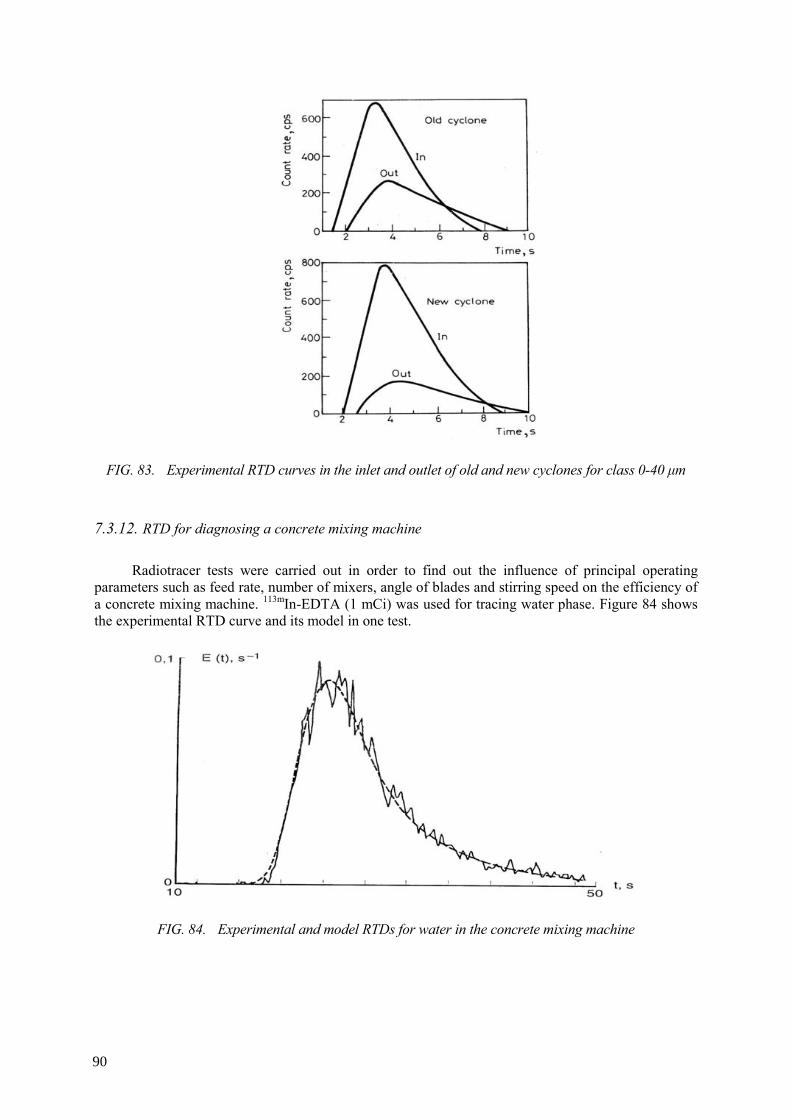
FIG. 83. Experimental RTD curves in the inlet and outlet of old and new cyclones for class 0-40 μm

7.3.12. RTD for diagnosing a concrete mixing machine

Radiotracer tests were carried out in order to find out the influence of principal operating

parameters such as feed rate, number of mixers, angle of blades and stirring speed on the efficiency of a concrete mixing machine. 113mIn-EDTA (1 mCi) was used for tracing water phase. Figure 84 shows the experimental RTD curve and its model in one test.

FIG. 84. Experimental and model RTDs for water in the concrete mixing machine

90

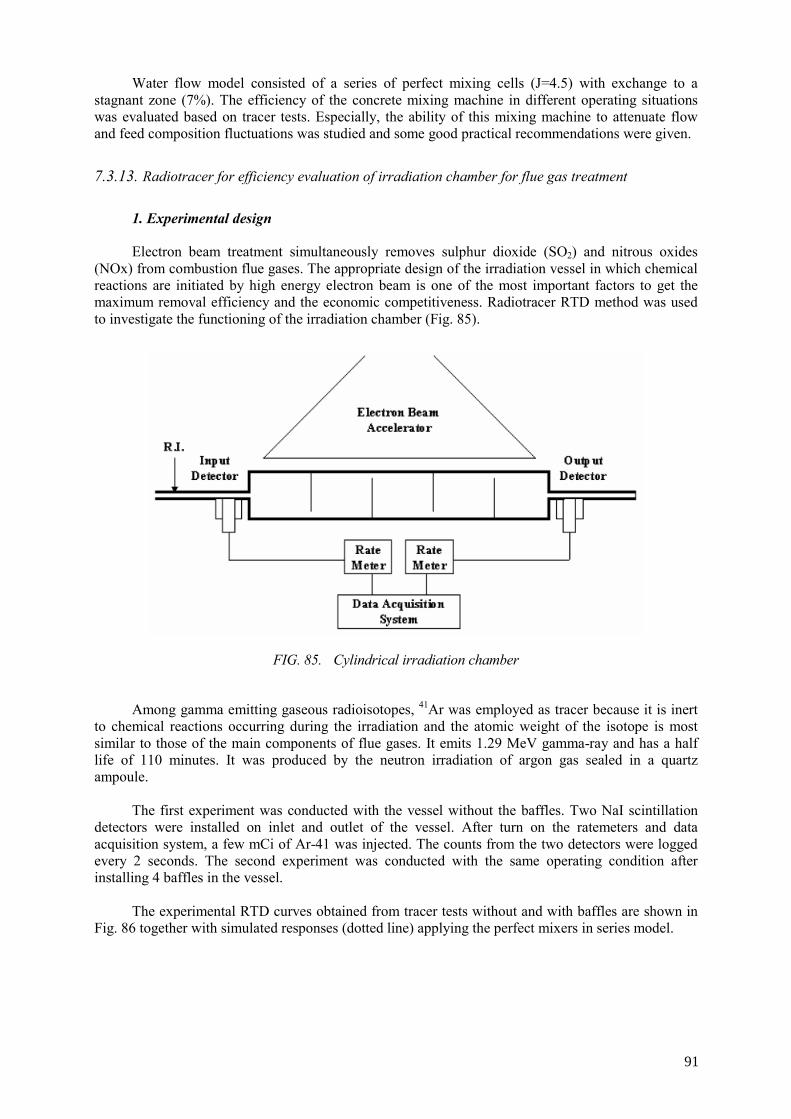
Water flow model consisted of a series of perfect mixing cells (J=4.5) with exchange to a stagnant zone (7%). The efficiency of the concrete mixing machine in different operating situations was evaluated based on tracer tests. Especially, the ability of this mixing machine to attenuate flow and feed composition fluctuations was studied and some good practical recommendations were given.

7.3.13. Radiotracer for efficiency evaluation of irradiation chamber for flue gas treatment

1. Experimental design Electron beam treatment simultaneously removes sulphur dioxide (SO2) and nitrous oxides

(NOx) from combustion flue gases. The appropriate design of the irradiation vessel in which chemical reactions are initiated by high energy electron beam is one of the most important factors to get the maximum removal efficiency and the economic competitiveness. Radiotracer RTD method was used to investigate the functioning of the irradiation chamber (Fig. 85).

FIG. 85. Cylindrical irradiation chamber

Among gamma emitting gaseous radioisotopes, 41Ar was employed as tracer because it is inert

to chemical reactions occurring during the irradiation and the atomic weight of the isotope is most similar to those of the main components of flue gases. It emits 1.29 MeV gamma-ray and has a half life of 110 minutes. It was produced by the neutron irradiation of argon gas sealed in a quartz ampoule.

The first experiment was conducted with the vessel without the baffles. Two NaI scintillation

detectors were installed on inlet and outlet of the vessel. After turn on the ratemeters and data acquisition system, a few mCi of Ar-41 was injected. The counts from the two detectors were logged every 2 seconds. The second experiment was conducted with the same operating condition after installing 4 baffles in the vessel.

The experimental RTD curves obtained from tracer tests without and with baffles are shown in

Fig. 86 together with simulated responses (dotted line) applying the perfect mixers in series model.

91

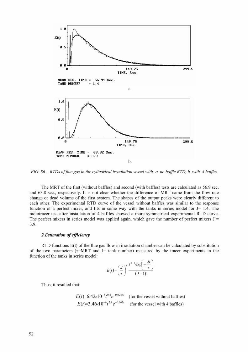
a.

b.

FIG. 86. RTDs of flue gas in the cylindrical irradiation vessel with: a. no baffle RTD, b. with 4 baffles

The MRT of the first (without baffles) and second (with baffles) tests are calculated as 56.9 sec.

and 63.8 sec., respectively. It is not clear whether the difference of MRT came from the flow rate change or dead volume of the first system. The shapes of the output peaks were clearly different to each other. The experimental RTD curve of the vessel without baffles was similar to the response function of a perfect mixer, and fits in some way with the tanks in series model for J= 1.4. The radiotracer test after installation of 4 baffles showed a more symmetrical experimental RTD curve. The perfect mixers in series model was applied again, which gave the number of perfect mixers J = 3.9.

2.Estimation of efficiency RTD functions E(t) of the flue gas flow in irradiation chamber can be calculated by substitution

of the two parameters (τ=MRT and J= tank number) measured by the tracer experiments in the function of the tanks in series model:

( ) ( )!1

exp1

−

⎟⎠⎞

⎜⎝⎛−

⎟⎠⎞

⎜⎝⎛=

−

J

JttJtE

JJ τ

τ

Thus, it resulted that:

tettE 0246.04.031042.6)( −−×= (for the vessel without baffles) tettE 061.09.261046.3)( −−×= (for the vessel with 4 baffles)

92

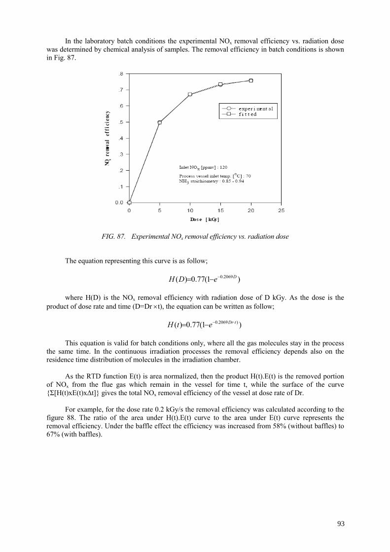
In the laboratory batch conditions the experimental NOx removal efficiency vs. radiation dose was determined by chemical analysis of samples. The removal efficiency in batch conditions is shown in Fig. 87.

FIG. 87. Experimental NOx removal efficiency vs. radiation dose

The equation representing this curve is as follow;

)1(77.0)( 2069.0 DeDH −−= where H(D) is the NOx removal efficiency with radiation dose of D kGy. As the dose is the

product of dose rate and time (D=Dr ×t), the equation can be written as follow;

)1(77.0)( )2069.0 tDretH ⋅−−= This equation is valid for batch conditions only, where all the gas molecules stay in the process

the same time. In the continuous irradiation processes the removal efficiency depends also on the residence time distribution of molecules in the irradiation chamber.

As the RTD function E(t) is area normalized, then the product H(t).E(t) is the removed portion

of NOx from the flue gas which remain in the vessel for time t, while the surface of the curve {Σ[H(t)xE(t)xΔt]} gives the total NOx removal efficiency of the vessel at dose rate of Dr.

For example, for the dose rate 0.2 kGy/s the removal efficiency was calculated according to the

figure 88. The ratio of the area under H(t).E(t) curve to the area under E(t) curve represents the removal efficiency. Under the baffle effect the efficiency was increased from 58% (without baffles) to 67% (with baffles).

93

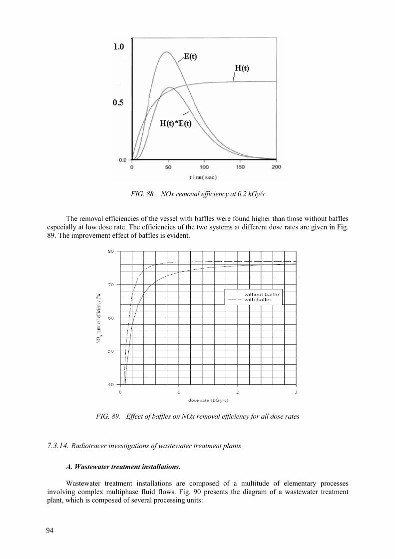
FIG. 88. NOx removal efficiency at 0.2 kGy/s

The removal efficiencies of the vessel with baffles were found higher than those without baffles

especially at low dose rate. The efficiencies of the two systems at different dose rates are given in Fig. 89. The improvement effect of baffles is evident.

FIG. 89. Effect of baffles on NOx removal efficiency for all dose rates

7.3.14. Radiotracer investigations of wastewater treatment plants

A. Wastewater treatment installations. Wastewater treatment installations are composed of a multitude of elementary processes

involving complex multiphase fluid flows. Fig. 90 presents the diagram of a wastewater treatment plant, which is composed of several processing units:

94

FIG. 90. A complete design of a typical wastewater treatment plant

The wastewater treatment installations work according to the following principles:

1. Preliminary treatment- screening of solid materials to remove large solid material such as paper, plastics, sand and silt. 2. Primary treatment: settling tank (primary clarifier) based on physical separation of solids and grease from the wastewater. Sludge is collected at the bottom and pumped to the digester. 3. Secondary treatment- biological aeration tank; air is blown for mixing and to promote the growth of micro-organisms which create a solid organic material (sludge= “active biomass” ) 4. Secondary clarifier

• sludge (biomass) settles under gravity to tank bottom and pumped to digester. • clarified wastewater passes through for Tertiary Treatment (disinfection; chlorine is

usually dosed into the treated wastewater stream for disinfection). 5. Sludge treatment – anaerobic process in digester: solids from settling tank and clarifier are sent to digesters for solids processing. Micro-organisms, called anaerobic bacteria, which do not need oxygen for growth, use the organic material present in the solids as a food source and convert it to by-products such as methane gas and water.

All these processes are presented schematically in the fig. 91.

95

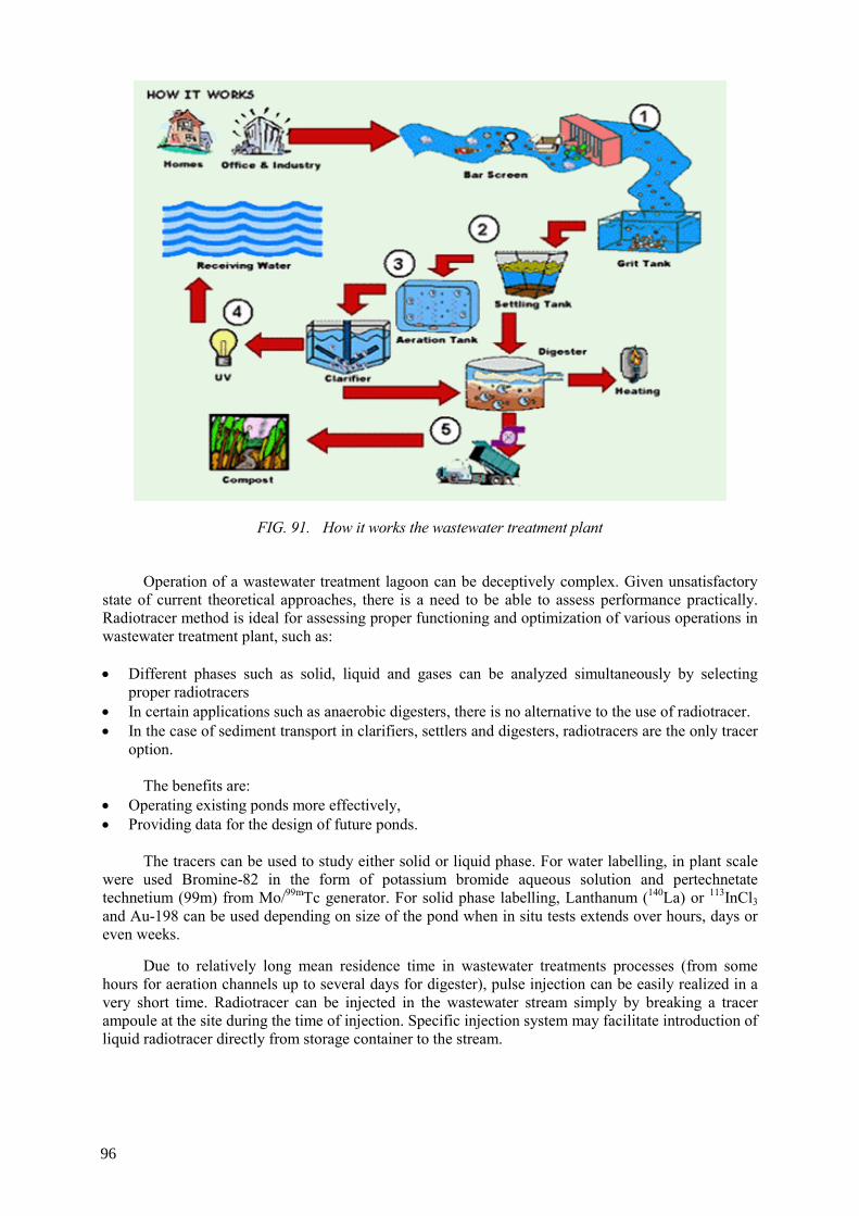
FIG. 91. How it works the wastewater treatment plant

Operation of a wastewater treatment lagoon can be deceptively complex. Given unsatisfactory

state of current theoretical approaches, there is a need to be able to assess performance practically. Radiotracer method is ideal for assessing proper functioning and optimization of various operations in wastewater treatment plant, such as:

• Different phases such as solid, liquid and gases can be analyzed simultaneously by selecting

proper radiotracers • In certain applications such as anaerobic digesters, there is no alternative to the use of radiotracer. • In the case of sediment transport in clarifiers, settlers and digesters, radiotracers are the only tracer

option. The benefits are:

• Operating existing ponds more effectively, • Providing data for the design of future ponds.

The tracers can be used to study either solid or liquid phase. For water labelling, in plant scale

were used Bromine-82 in the form of potassium bromide aqueous solution and pertechnetate technetium (99m) from Mo/99mTc generator. For solid phase labelling, Lanthanum (140La) or 113InCl3 and Au-198 can be used depending on size of the pond when in situ tests extends over hours, days or even weeks.

Due to relatively long mean residence time in wastewater treatments processes (from some

hours for aeration channels up to several days for digester), pulse injection can be easily realized in a very short time. Radiotracer can be injected in the wastewater stream simply by breaking a tracer ampoule at the site during the time of injection. Specific injection system may facilitate introduction of liquid radiotracer directly from storage container to the stream.

96

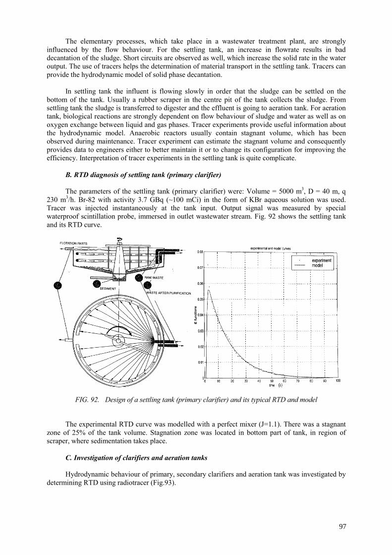
The elementary processes, which take place in a wastewater treatment plant, are strongly influenced by the flow behaviour. For the settling tank, an increase in flowrate results in bad decantation of the sludge. Short circuits are observed as well, which increase the solid rate in the water output. The use of tracers helps the determination of material transport in the settling tank. Tracers can provide the hydrodynamic model of solid phase decantation.

In settling tank the influent is flowing slowly in order that the sludge can be settled on the

bottom of the tank. Usually a rubber scraper in the centre pit of the tank collects the sludge. From settling tank the sludge is transferred to digester and the effluent is going to aeration tank. For aeration tank, biological reactions are strongly dependent on flow behaviour of sludge and water as well as on oxygen exchange between liquid and gas phases. Tracer experiments provide useful information about the hydrodynamic model. Anaerobic reactors usually contain stagnant volume, which has been observed during maintenance. Tracer experiment can estimate the stagnant volume and consequently provides data to engineers either to better maintain it or to change its configuration for improving the efficiency. Interpretation of tracer experiments in the settling tank is quite complicate.

B. RTD diagnosis of settling tank (primary clarifier) The parameters of the settling tank (primary clarifier) were: Volume = 5000 m3, D = 40 m, q

230 m3/h. Br-82 with activity 3.7 GBq (~100 mCi) in the form of KBr aqueous solution was used. Tracer was injected instantaneously at the tank input. Output signal was measured by special waterproof scintillation probe, immersed in outlet wastewater stream. Fig. 92 shows the settling tank and its RTD curve.

FIG. 92. Design of a settling tank (primary clarifier) and its typical RTD and model

The experimental RTD curve was modelled with a perfect mixer (J=1.1). There was a stagnant

zone of 25% of the tank volume. Stagnation zone was located in bottom part of tank, in region of scraper, where sedimentation takes place.

C. Investigation of clarifiers and aeration tanks Hydrodynamic behaviour of primary, secondary clarifiers and aeration tank was investigated by

determining RTD using radiotracer (Fig.93).

97

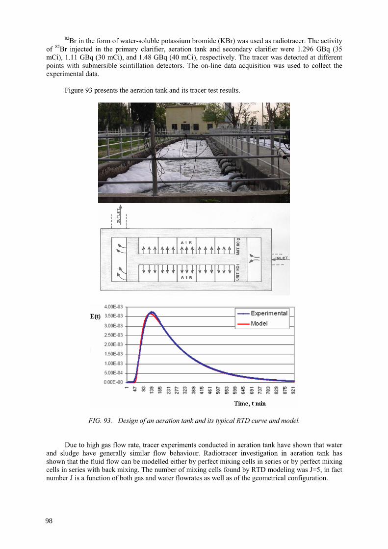
82Br in the form of water-soluble potassium bromide (KBr) was used as radiotracer. The activity of 82Br injected in the primary clarifier, aeration tank and secondary clarifier were 1.296 GBq (35 mCi), 1.11 GBq (30 mCi), and 1.48 GBq (40 mCi), respectively. The tracer was detected at different points with submersible scintillation detectors. The on-line data acquisition was used to collect the experimental data.

Figure 93 presents the aeration tank and its tracer test results.

FIG. 93. Design of an aeration tank and its typical RTD curve and model.

Due to high gas flow rate, tracer experiments conducted in aeration tank have shown that water

and sludge have generally similar flow behaviour. Radiotracer investigation in aeration tank has shown that the fluid flow can be modelled either by perfect mixing cells in series or by perfect mixing cells in series with back mixing. The number of mixing cells found by RTD modeling was J=5, in fact number J is a function of both gas and water flowrates as well as of the geometrical configuration.

98

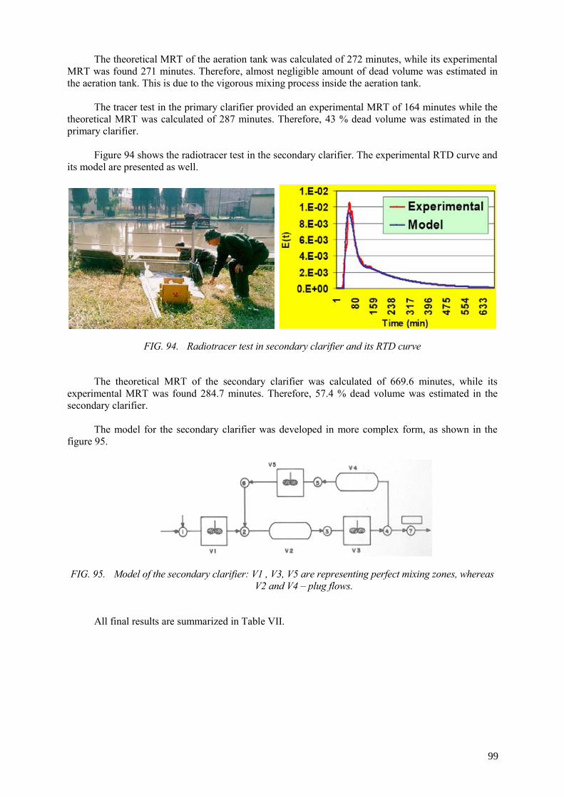
The theoretical MRT of the aeration tank was calculated of 272 minutes, while its experimental MRT was found 271 minutes. Therefore, almost negligible amount of dead volume was estimated in the aeration tank. This is due to the vigorous mixing process inside the aeration tank.

The tracer test in the primary clarifier provided an experimental MRT of 164 minutes while the

theoretical MRT was calculated of 287 minutes. Therefore, 43 % dead volume was estimated in the primary clarifier.

Figure 94 shows the radiotracer test in the secondary clarifier. The experimental RTD curve and

its model are presented as well.

FIG. 94. Radiotracer test in secondary clarifier and its RTD curve

The theoretical MRT of the secondary clarifier was calculated of 669.6 minutes, while its

experimental MRT was found 284.7 minutes. Therefore, 57.4 % dead volume was estimated in the secondary clarifier.

The model for the secondary clarifier was developed in more complex form, as shown in the

figure 95.

FIG. 95. Model of the secondary clarifier: V1 , V3, V5 are representing perfect mixing zones, whereas V2 and V4 – plug flows.

All final results are summarized in Table VII.

99

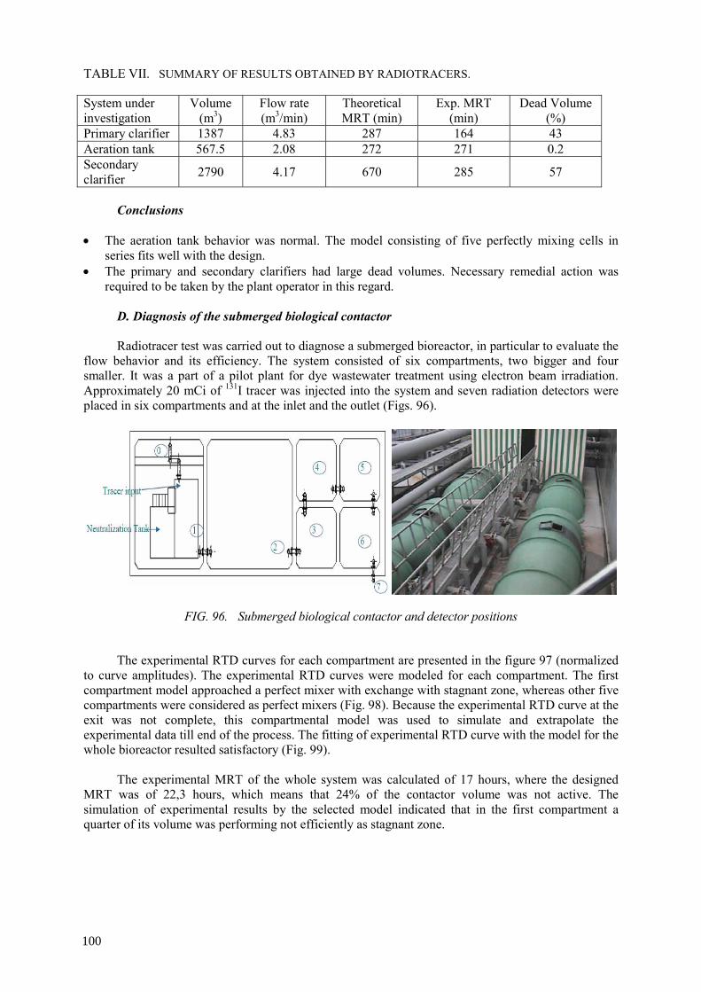
TABLE VII. SUMMARY OF RESULTS OBTAINED BY RADIOTRACERS.

System under investigation

Volume (m3)

Flow rate (m3/min)

Theoretical MRT (min)

Exp. MRT (min)

Dead Volume (%)

Primary clarifier 1387 4.83 287 164 43 Aeration tank 567.5 2.08 272 271 0.2 Secondary clarifier 2790 4.17 670 285 57

Conclusions

• The aeration tank behavior was normal. The model consisting of five perfectly mixing cells in series fits well with the design.

• The primary and secondary clarifiers had large dead volumes. Necessary remedial action was required to be taken by the plant operator in this regard.

D. Diagnosis of the submerged biological contactor Radiotracer test was carried out to diagnose a submerged bioreactor, in particular to evaluate the

flow behavior and its efficiency. The system consisted of six compartments, two bigger and four smaller. It was a part of a pilot plant for dye wastewater treatment using electron beam irradiation. Approximately 20 mCi of 131I tracer was injected into the system and seven radiation detectors were placed in six compartments and at the inlet and the outlet (Figs. 96).

FIG. 96. Submerged biological contactor and detector positions

The experimental RTD curves for each compartment are presented in the figure 97 (normalized

to curve amplitudes). The experimental RTD curves were modeled for each compartment. The first compartment model approached a perfect mixer with exchange with stagnant zone, whereas other five compartments were considered as perfect mixers (Fig. 98). Because the experimental RTD curve at the exit was not complete, this compartmental model was used to simulate and extrapolate the experimental data till end of the process. The fitting of experimental RTD curve with the model for the whole bioreactor resulted satisfactory (Fig. 99).

The experimental MRT of the whole system was calculated of 17 hours, where the designed

MRT was of 22,3 hours, which means that 24% of the contactor volume was not active. The simulation of experimental results by the selected model indicated that in the first compartment a quarter of its volume was performing not efficiently as stagnant zone.

100

FIG. 97. Experimental RTD curves measured at each compartment

FIG. 98. Model of the flow in the whole bioreactor

FIG. 99. The model and the experimental data for the whole bioreactor.

The cumulative RTD function F(t) was calculated for each compartment from simulated

experimental RTD curves (Fig. 100). The F(t) function specifies the traced material flowing out the tank after the time t. This function provides also the sampling time at the outlet of each tank for the same irradiation regime. This was an important parameter of the whole irradiation facility for performing representative samplings after every change of operational condition of the electron beam accelerator. Representative samplings were necessary for reliable data of the treatment process efficiency and scaling up the pilot plant results.

101

FIG. 100. Calculation of the sampling time (flowing out time) in each tank

The results of the radiotracer tests helped the designer of the wastewater treatment irradiation

plant to schedule suitable sampling times for each compartment in function of the irradiation operation conditions.

E. Diagnosis of sludge digester a. Problem Sludge collected during the treatment process contains a large amount of biodegradable material

making it amenable to treatment by a different set of micro-organisms, called anaerobic bacteria, which do not need oxygen for growth. Sludge treatment in digester is an anaerobic process. During this process, micro-organisms use the organic material present in the solids as a food source and convert it to by-products such as methane gas and water. This takes place in special fully enclosed digesters heated to 35 degrees Celsius, where these anaerobic micro-organisms thrive without any oxygen. Digestion results in a 90% reduction of pathogens and the production of a wet soil-like material called "biosolids" that contain 95-97% water.

The role of the digester unit in a wastewater treatment plant is to:

• Reduce the organic contents of sludge by biological decomposition process, • Produce CH4 that can be used for heating the digester itself for microorganism. • Contribute to save the cost for waste treatment by reducing volume of waste solid.

Operation efficiency of digester is determined by

• Condition of microorganism consuming sludge • Chemical composition of sludge • Dynamic characteristic of the sludge.

Although some natural mixing occurs in an anaerobic digester because of rising sludge gas

bubbles and the thermal convection currents caused by the addition of heat, these levels of mixing are not adequate to ensure stable digestion process performance at high loading rates. Poor quality of digested sludge is a common and often problem in practice. Fig. 101 shows typical oval and cylindrical sludge digesters commonly used in most part of wastewater treatment plants.

102

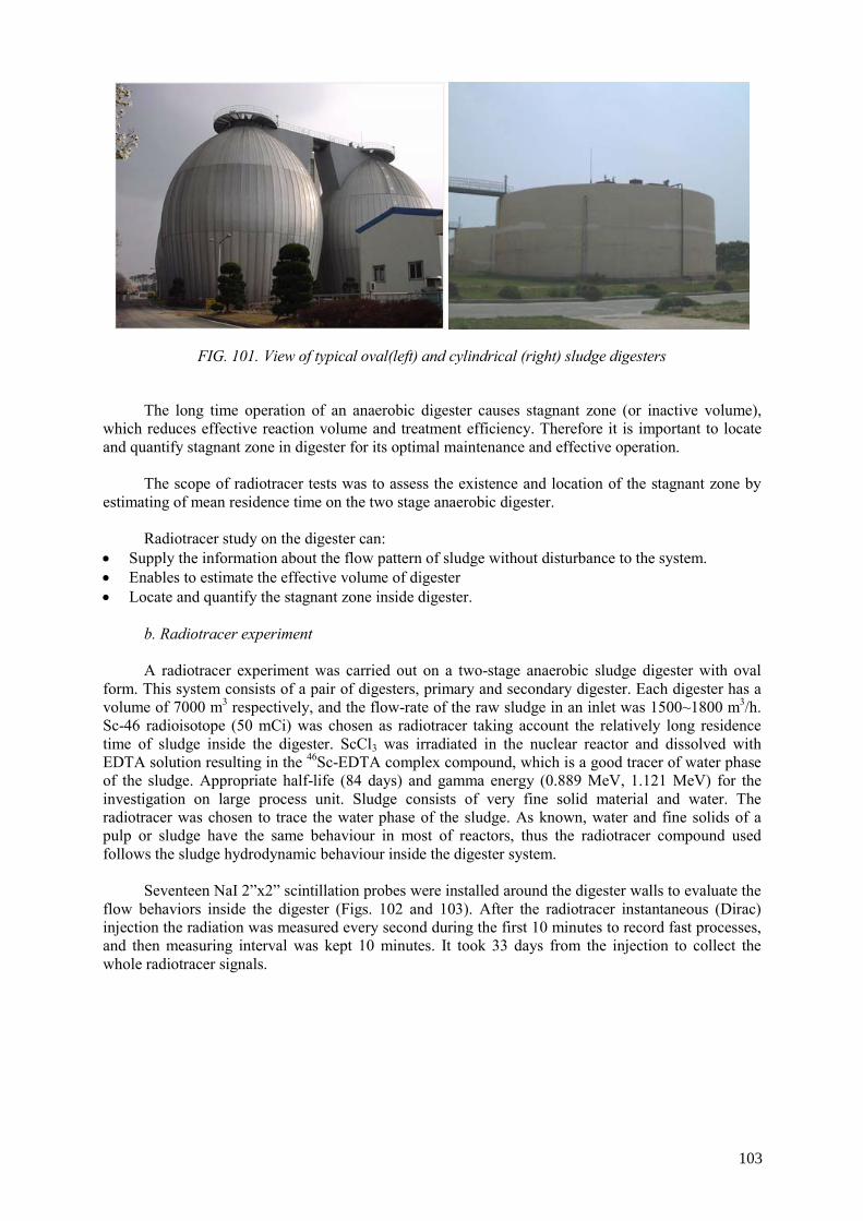
FIG. 101. View of typical oval(left) and cylindrical (right) sludge digesters

The long time operation of an anaerobic digester causes stagnant zone (or inactive volume),

which reduces effective reaction volume and treatment efficiency. Therefore it is important to locate and quantify stagnant zone in digester for its optimal maintenance and effective operation.

The scope of radiotracer tests was to assess the existence and location of the stagnant zone by

estimating of mean residence time on the two stage anaerobic digester. Radiotracer study on the digester can:

• Supply the information about the flow pattern of sludge without disturbance to the system. • Enables to estimate the effective volume of digester • Locate and quantify the stagnant zone inside digester.

b. Radiotracer experiment A radiotracer experiment was carried out on a two-stage anaerobic sludge digester with oval

form. This system consists of a pair of digesters, primary and secondary digester. Each digester has a volume of 7000 m3 respectively, and the flow-rate of the raw sludge in an inlet was 1500~1800 m3/h. Sc-46 radioisotope (50 mCi) was chosen as radiotracer taking account the relatively long residence time of sludge inside the digester. ScCl3 was irradiated in the nuclear reactor and dissolved with EDTA solution resulting in the 46Sc-EDTA complex compound, which is a good tracer of water phase of the sludge. Appropriate half-life (84 days) and gamma energy (0.889 MeV, 1.121 MeV) for the investigation on large process unit. Sludge consists of very fine solid material and water. The radiotracer was chosen to trace the water phase of the sludge. As known, water and fine solids of a pulp or sludge have the same behaviour in most of reactors, thus the radiotracer compound used follows the sludge hydrodynamic behaviour inside the digester system.

Seventeen NaI 2”x2” scintillation probes were installed around the digester walls to evaluate the

flow behaviors inside the digester (Figs. 102 and 103). After the radiotracer instantaneous (Dirac) injection the radiation was measured every second during the first 10 minutes to record fast processes, and then measuring interval was kept 10 minutes. It took 33 days from the injection to collect the whole radiotracer signals.

103

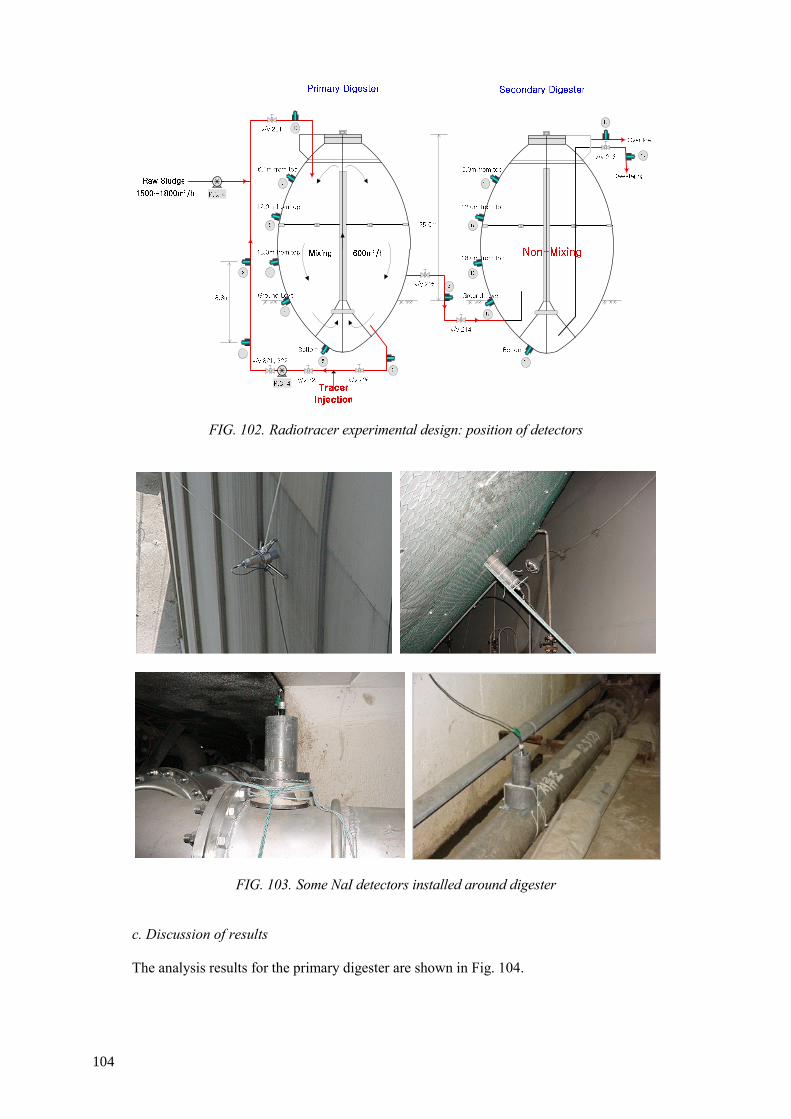
FIG. 102. Radiotracer experimental design: position of detectors

FIG. 103. Some NaI detectors installed around digester

c. Discussion of results The analysis results for the primary digester are shown in Fig. 104.

104

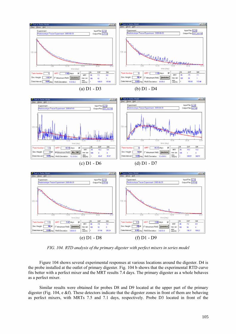
(a) D1 - D3 (b) D1 - D4

(c) D1 - D6 (d) D1 - D7

(e) D1 - D8 (f) D1 - D9

FIG. 104. RTD analysis of the primary digester with perfect mixers in series model

Figure 104 shows several experimental responses at various locations around the digester. D4 is

the probe installed at the outlet of primary digester. Fig. 104 b shows that the experimental RTD curve fits better with a perfect mixer and the MRT results 7.4 days. The primary digester as a whole behaves as a perfect mixer.

Similar results were obtained for probes D8 and D9 located at the upper part of the primary

digester (Fig. 104, e &f). These detectors indicate that the digester zones in front of them are behaving as perfect mixers, with MRTs 7.5 and 7.1 days, respectively. Probe D3 located in front of the

105

recirculation flow also indicates a perfect mixing zone in front of it (Fig. 104, a), with a MRT of 7 days. As shown above the parameters of flow dynamics provided by probes D3, D4, D8 and D9 are almost the same.

However, detector D6 and D7 located on the lower part of a digester showed different flow

patterns from those of probes in the upper part of digester (D8 and D9). Intensity of radiation detected by probes D6 and D7 was substantially lower than those of the detectors in the upper part of the primary digester. At the beginning (after radiotracer injection), D6 and D7 showed no radiation indication, and later on tracer appeared reaching a peak. After the peak, the curves decreased exponentially with time having a long tail, which indicates the presence of stagnant zones in these parts of the digester. Because of the stagnant zones, the MRTs of sludge in zones in front of probes D6 and D7 were found, of 10.2 and 15.2 days, respectively (higher than the theoretical MRT of the primary digester). The probe D5 placed at the bottom part of the digester did not show any tracer signal at all during the experiment duration. This indicates the presence of a sludge scale layer in this part of digester (7~9 m above the ground level from the bottom).

Using the signal of the detector D4 as an inflow a similar analysis was carried out for the

secondary digester. The results of the secondary digester are shown in Fig. 105.

(a) D4 - D12

(b) D4 - D16 (c) D1 - D16

FIG. 105. RTD analysis of the secondary digester

The secondary digester has no mixing facility and functions only to separate the mixed sludge

being delivered from the primary digester statically.

106

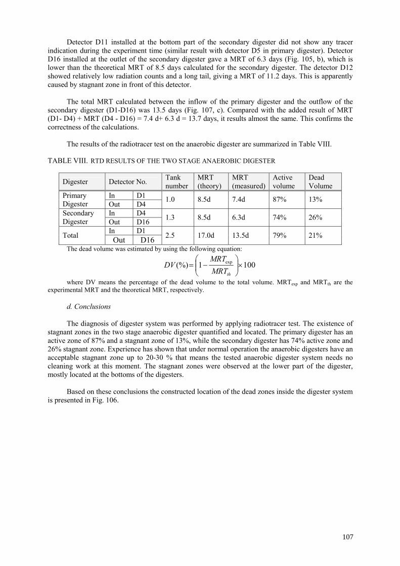
Detector D11 installed at the bottom part of the secondary digester did not show any tracer indication during the experiment time (similar result with detector D5 in primary digester). Detector D16 installed at the outlet of the secondary digester gave a MRT of 6.3 days (Fig. 105, b), which is lower than the theoretical MRT of 8.5 days calculated for the secondary digester. The detector D12 showed relatively low radiation counts and a long tail, giving a MRT of 11.2 days. This is apparently caused by stagnant zone in front of this detector.

The total MRT calculated between the inflow of the primary digester and the outflow of the

secondary digester (D1-D16) was 13.5 days (Fig. 107, c). Compared with the added result of MRT (D1- D4) + MRT (D4 - D16) = 7.4 d+ 6.3 d = 13.7 days, it results almost the same. This confirms the correctness of the calculations.

The results of the radiotracer test on the anaerobic digester are summarized in Table VIII.

TABLE VIII. RTD RESULTS OF THE TWO STAGE ANAEROBIC DIGESTER

Digester Detector No. Tank number

MRT (theory)

MRT (measured)

Active volume

Dead Volume

In D1 Primary Digester Out D4

1.0 8.5d 7.4d 87% 13%

In D4 Secondary Digester Out D16 1.3 8.5d 6.3d 74% 26%

In D1 Total Out D16 2.5 17.0d 13.5d 79% 21%

The dead volume was estimated by using the following equation:

1001(%) exp ×⎟⎟⎠

⎞⎜⎜⎝

⎛−=

thMRTMRT

DV

where DV means the percentage of the dead volume to the total volume. MRTexp and MRTth are the experimental MRT and the theoretical MRT, respectively.

d. Conclusions The diagnosis of digester system was performed by applying radiotracer test. The existence of

stagnant zones in the two stage anaerobic digester quantified and located. The primary digester has an active zone of 87% and a stagnant zone of 13%, while the secondary digester has 74% active zone and 26% stagnant zone. Experience has shown that under normal operation the anaerobic digesters have an acceptable stagnant zone up to 20-30 % that means the tested anaerobic digester system needs no cleaning work at this moment. The stagnant zones were observed at the lower part of the digester, mostly located at the bottoms of the digesters.

Based on these conclusions the constructed location of the dead zones inside the digester system

107

is presented in Fig. 106.

F. Wastewater chlorinate for purifying Chlorine is normally used for water disinfection. The chlorine reactor consisted of two

cylindrical reservoirs connected in series with volumes of V1 = 925 m3 and V2 = 1625 m3 (Fig. 107). The mean residence time of water flow across both reservoirs was estimated of several hours.

FIG. 107. Reactor of water chlorification: before modification (up); after modifications (down)

108

FIG. 106. The location of stagnant zones in the digester system.

The main problem suspected was the low efficiency of wastewater chlorinate process. It was assumed the generation of preferential flows and the creation of dead volumes. The purpose of the radiotracer tests was to diagnose the water phase hydrodynamic, to find out the actual model of transport (plug flow model was preferred), to evaluate the reactor efficiency and probably to optimize it. There were performed two radiotracer tests, a first as it was, and the second on after modification of reservoirs design (installation of baffles).

99mTc radiotracer (60 mCi) was used for each test. The experimental RTD curves and their

models are shown in fig. 108.

FIG. 108. Experimental RTD curves and their models before(left) and after (right) modification

The experimental RTD curve of first test was better approached by the model of two perfect

mixers in series (J=2) with some exchange with stagnant volume. The stagnant volume was estimated of 2-3 %, so rather small for affecting the performance and efficiency of the existing reactor. Near perfect mixer model provides for rather bad and non-uniform micromixing of water with chlorine because of very large range of water residence times, so the purifying process was not efficient.

Installation of baffles inside the reactor was proposed to remediate the situation and improve the

efficiency. The radiotracer test after installation of baffles showed a symmetrical experimental RTD curve (Fig. 108, right). The perfect mixers in series model was applied again but in this case the number of perfect mixers resulted of J = 20, that means the water is moving almost as plug flow. The micromixing is improved and consequently the efficiency of disinfectation was considerably increased.

7.3.15. Radiotracers for flow meter calibration

Transit time method is commonly used in calibrating flow meters in processing pipes in closed

conduits. The responses to tracer instantaneous (Dirac) injection in two sections of the pipes are recorded. The responses in fact are not strictly RTD curves but are considered as such. The error of two MRTs calculated from the experimental RTD curves obtained in two sections is crucial for the accuracy of whole flow rate measurement.

The data acquisition system has normally a measuring time 1-2 ms in order to respond to fast

transit of flows in front of detector. This technique is already accepted as standard for flow meter calibration in several countries. Better than 1% accuracy is achievable. The distance between injection and measuring sections should be great enough to achieve adequate mixing of the tracer with the water flowing in the conduit.

A. Gas flowmeter calibration Radiotracer technique, using the Kr-85 radioisotope in gaseous form, was applied for the

calibration of air flow measuring system in shaft furnace of copper production. In the shaft process of

109

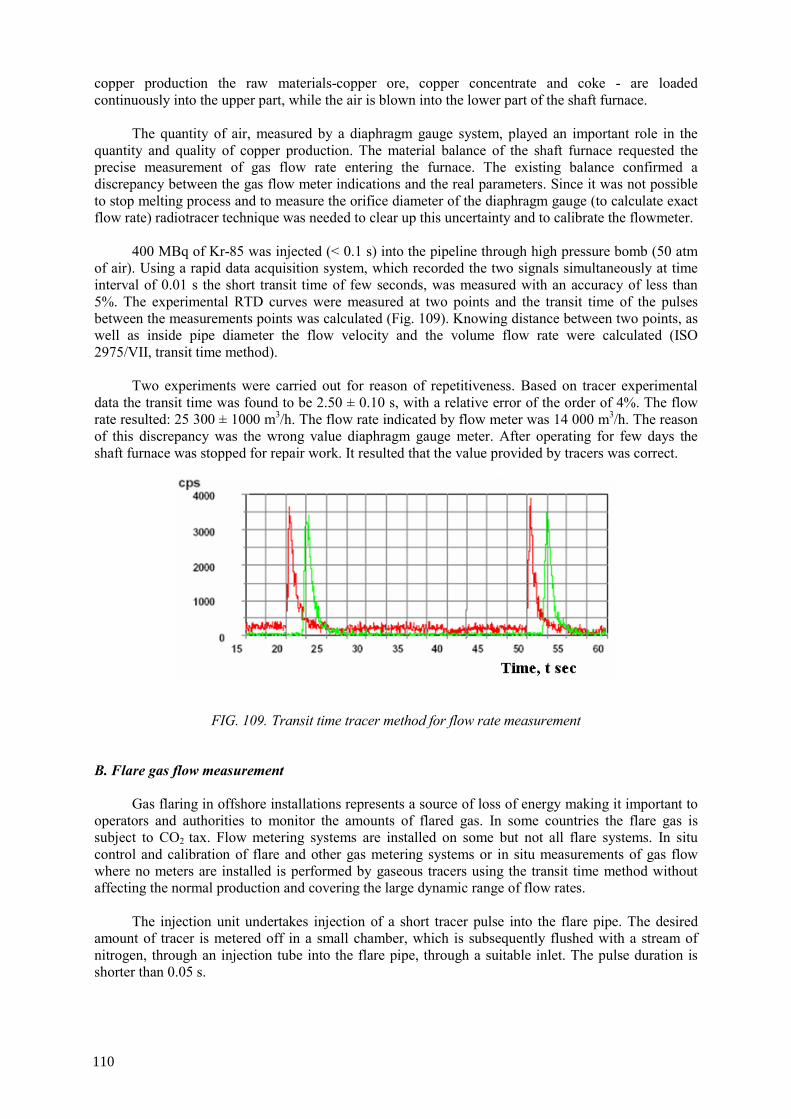
copper production the raw materials-copper ore, copper concentrate and coke - are loaded continuously into the upper part, while the air is blown into the lower part of the shaft furnace.

The quantity of air, measured by a diaphragm gauge system, played an important role in the quantity and quality of copper production. The material balance of the shaft furnace requested the precise measurement of gas flow rate entering the furnace. The existing balance confirmed a discrepancy between the gas flow meter indications and the real parameters. Since it was not possible to stop melting process and to measure the orifice diameter of the diaphragm gauge (to calculate exact flow rate) radiotracer technique was needed to clear up this uncertainty and to calibrate the flowmeter.

400 MBq of Kr-85 was injected (< 0.1 s) into the pipeline through high pressure bomb (50 atm

of air). Using a rapid data acquisition system, which recorded the two signals simultaneously at time interval of 0.01 s the short transit time of few seconds, was measured with an accuracy of less than 5%. The experimental RTD curves were measured at two points and the transit time of the pulses between the measurements points was calculated (Fig. 109). Knowing distance between two points, as well as inside pipe diameter the flow velocity and the volume flow rate were calculated (ISO 2975/VII, transit time method).

Two experiments were carried out for reason of repetitiveness. Based on tracer experimental

data the transit time was found to be 2.50 ± 0.10 s, with a relative error of the order of 4%. The flow rate resulted: 25 300 ± 1000 m3/h. The flow rate indicated by flow meter was 14 000 m3/h. The reason of this discrepancy was the wrong value diaphragm gauge meter. After operating for few days the shaft furnace was stopped for repair work. It resulted that the value provided by tracers was correct.

FIG. 109. Transit time tracer method for flow rate measurement

B. Flare gas flow measurement

Gas flaring in offshore installations represents a source of loss of energy making it important to

operators and authorities to monitor the amounts of flared gas. In some countries the flare gas is subject to CO2 tax. Flow metering systems are installed on some but not all flare systems. In situ control and calibration of flare and other gas metering systems or in situ measurements of gas flow where no meters are installed is performed by gaseous tracers using the transit time method without affecting the normal production and covering the large dynamic range of flow rates.

The injection unit undertakes injection of a short tracer pulse into the flare pipe. The desired

amount of tracer is metered off in a small chamber, which is subsequently flushed with a stream of nitrogen, through an injection tube into the flare pipe, through a suitable inlet. The pulse duration is shorter than 0.05 s.

110

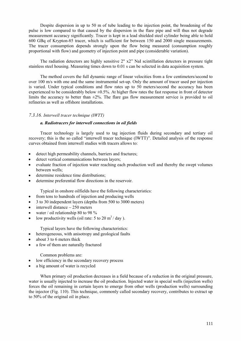
Despite dispersion in up to 50 m of tube leading to the injection point, the broadening of the pulse is low compared to that caused by the dispersion in the flare pipe and will thus not degrade measurement accuracy significantly. Tracer is kept in a lead shielded steel cylinder being able to hold 600 GBq of Krypton-85 tracer, which is sufficient for between 150 and 2000 single measurements. The tracer consumption depends strongly upon the flow being measured (consumption roughly proportional with flow) and geometry of injection point and pipe (considerable variation).

The radiation detectors are highly sensitive 2" x2” NaI scintillation detectors in pressure tight stainless steel housing. Measuring times down to 0.01 s can be selected in data acquisition system.

The method covers the full dynamic range of linear velocities from a few centimeters/second to

over 100 m/s with one and the same instrumental set-up. Only the amount of tracer used per injection is varied. Under typical conditions and flow rates up to 50 meters/second the accuracy has been experienced to be considerably below ±0.5%. At higher flow rates the fast response in front of detector limits the accuracy to better than ±2%. The flare gas flow measurement service is provided to oil refineries as well as offshore installations.

7.3.16. Interwell tracer technique (IWTT)

a. Radiotracers for interwell connections in oil fields Tracer technology is largely used to tag injection fluids during secondary and tertiary oil

recovery; this is the so called “interwell tracer technique (IWTT)”. Detailed analysis of the response curves obtained from interwell studies with tracers allows to:

• detect high permeability channels, barriers and fractures; • detect vertical communications between layers; • evaluate fraction of injection water reaching each production well and thereby the swept volumes

between wells; • determine residence time distributions; • determine preferential flow directions in the reservoir.

Typical in onshore oilfields have the following characteristics:

• from tens to hundreds of injection and producing wells • 3 to 30 independent layers (depths from 500 to 3000 meters) • interwell distance ~ 250 meters • water / oil relationship 80 to 98 % • low productivity wells (oil rate: 5 to 20 m3 / day ).

Typical layers have the following characteristics:

• heterogeneous, with anisotropy and geological faults • about 3 to 6 meters thick • a few of them are naturally fractured

Common problems are:

• low efficiency in the secondary recovery process • a big amount of water is recycled

When primary oil production decreases in a field because of a reduction in the original pressure,

water is usually injected to increase the oil production. Injected water in special wells (injection wells) forces the oil remaining in certain layers to emerge from other wells (production wells) surrounding the injector (Fig. 110). This technique, commonly called secondary recovery, contributes to extract up to 50% of the original oil in place.

111

FIG. 110. Interwell communication principle

Radioactive tracers have been used to great effect in enhancing oil production in oil fields. The

tracer method provides direct information, giving the transit times and water distribution percentages among the producing wells. The main radiotracer technique is the measuring of the “time of travel” between injection and production wells. Subsequent analysis of samples taken from surrounding production wells makes it possible to obtain the response curves of the tracer (concentration vs. time), which represent the dynamic flow behavior of the pattern (injector plus producers) under study.

b. Tracer injection Instantaneous injection of tracer (Tritium) is performed; this means the tracer is injected in few

FIG. 111. Tritium injection using bypass technique.

c. Tracer sampling Sampling program is very important in oilfield tracer tests (Fig. 112). It is strongly

recommended to start sampling right after tracer injection. Frequency of taking samples changes with the nature of oil reservoir. It depends on estimation of how fast injected water moves through reservoir. The faster the movement of injected water the higher the sampling frequency must be. It is critical to collect enough samples to catch the tracer breakthrough time and obtain the whole response curve as fine as possible. After reaching the breakthrough, sampling frequency can be slowed down.

112

seconds using bypass or other injection techniques (Fig. 111).

FIG. 112. Sampling from a production well

d. Tracer data processing and interpretation. There are several levels of data processing and interpretation. First level or direct interpretation is as follows:

• Arrival time (tracer breakthrough). • Mean residence time • Percentage of the recovered tracer activity • Geological maps with tracer distribution data

Second level interpretation

• Analytical models matching • Finite difference numerical model matching • Finite element numerical model matching • Stream line model matching.

The time response to the instantaneous injection of the tracer in the injection well is the so

called “residence time distribution” of the tracer in the production well (Figs.113-114). In fact the tracer response profile in the production well is not exactly the classical RTD of a chemical engineering reactor because the tracer balance normally is not known and is out of control. But in practice the response curve in the production well is considered as the RTD of the zone injector-producer and may be proceeded in the same way like reactor RTD.

Normally, it takes typically several months to complete a measurement. If a water injection is to

be effective in sweeping out oil from the permeable zones it is important to ensure that short-circuiting or channeling, whereby much of the residual oil may be bypassed, does not occur. Therefore, it is important to understand how the water from injection well travels to the producer.

113

FIG. 113. Tracer dispersion (experimental “RTD”) curve in production well with rapid breakthrough and strong channelling.

a.

b.

FIG. 114. Experimental “RTD” curves in production well with normal dispersion and relatively slow breakthrough, 100 (a) and 300 (b) days, respectively

The tracer quantity recovered in the production wells around the injector normally is much less

than the tracer injected in the injection well. Typical tracer recoveries are several percents; in uniform small fields could happen that the recovery goes till 60-70 %, but there are cases, in particular in very fractioned and non-homogeneous structures that recovery less than 1% is found.

114

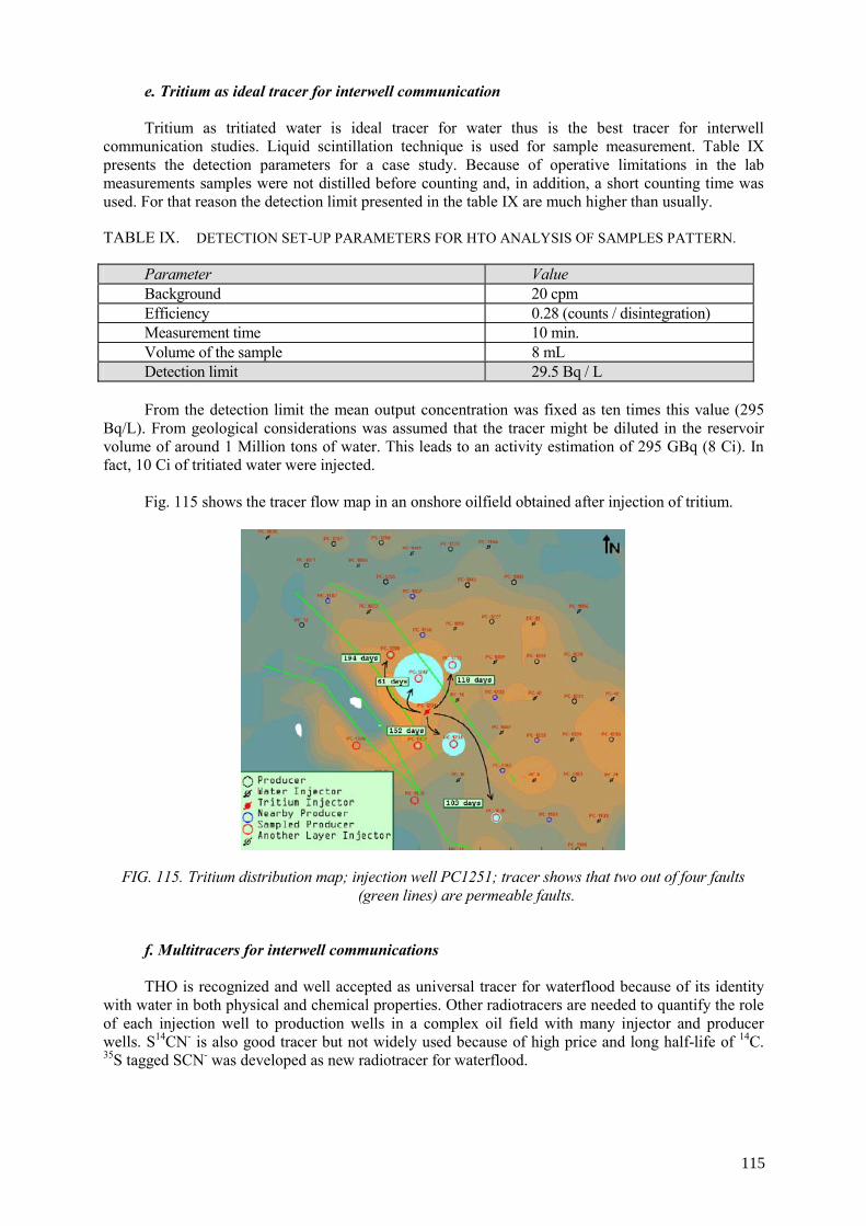
e. Tritium as ideal tracer for interwell communication Tritium as tritiated water is ideal tracer for water thus is the best tracer for interwell

communication studies. Liquid scintillation technique is used for sample measurement. Table IX presents the detection parameters for a case study. Because of operative limitations in the lab measurements samples were not distilled before counting and, in addition, a short counting time was used. For that reason the detection limit presented in the table IX are much higher than usually.

TABLE IX. DETECTION SET-UP PARAMETERS FOR HTO ANALYSIS OF SAMPLES PATTERN.

Parameter Value Background 20 cpm Efficiency 0.28 (counts / disintegration) Measurement time 10 min. Volume of the sample 8 mL Detection limit 29.5 Bq / L From the detection limit the mean output concentration was fixed as ten times this value (295

Bq/L). From geological considerations was assumed that the tracer might be diluted in the reservoir volume of around 1 Million tons of water. This leads to an activity estimation of 295 GBq (8 Ci). In fact, 10 Ci of tritiated water were injected.

Fig. 115 shows the tracer flow map in an onshore oilfield obtained after injection of tritium.

FIG. 115. Tritium distribution map; injection well PC1251; tracer shows that two out of four faults (green lines) are permeable faults.

f. Multitracers for interwell communications THO is recognized and well accepted as universal tracer for waterflood because of its identity

with water in both physical and chemical properties. Other radiotracers are needed to quantify the role of each injection well to production wells in a complex oil field with many injector and producer wells. S14CN- is also good tracer but not widely used because of high price and long half-life of 14C. 35S tagged SCN- was developed as new radiotracer for waterflood.

115

35S is a beta emitter with half-live of 87 days. 35S tagged SCN- can be used in reservoir with relatively quick breakthrough of water, such as reservoir of long water flooding history. 60Co tagged K3[Co(CN)6] is a good water tracer for IWTT studies. But, radiation hazard of 60Co limits its use and, in fact 60Co tagged K3[Co(CN)6] is replaced by 58Co, which has a half-life of 67.8 days only.

30 Ci of THO, 1.0 Ci of 35S-KSCN and 1.0 Ci of Co-58 tagged K3[Co(CN)6 were injected

separately as tracers into three injection wells (15-24, 14-26 and 13-26). The test lasted one year and its purpose was to evaluate water flooding performance and quantify the role of three injectors to 11 producer wells namely, 12-25, 13-25, 14-25, 15-25, 14-23, 13-28, L38, 14-27, 15-23, 16-25 and 15-27. Tracers were found in producer wells successively. Well position and tracer movement directions are shown in the oil field map below (Fig. 117). The tracer movement map showed clearly that each of the tracers was found during the test period. In the producer well 14-25 three tracers were found. It means that water produced in well 14-25 contains contribution from the three injection wells 15-24, 14-26 and 13-26. In three producer wells 15-25, 14-27 and 13-25 two kinds of tracers were found.

35SCN- injected in the well 13-26 was found in the production wells 13-28 and 12-25. This

important result has proved that the faults located between injection and production wells are not a barrier for water movement (Fig. 116).

FIG. 116. Wells pattern and tracer movement in multitracer test

g. Conclusions Typical conclusions from the IWTT:

• tracer arrival time and mean residence times can go from few day to many months, • geological faults can not be generalized as always impermeable ones; there are permeable faults as

well that means oil and water move through them. Practical value of tracer tests could be also:

• shutoff of highly watered zones; • better planning of injection and production wells configuration.

Although this technique was firstly used in old reservoirs, in which oil production had

decreased, it is today a common practice to begin the exploitation of new wells with fluid injection as a way to optimize oil recovery.

116

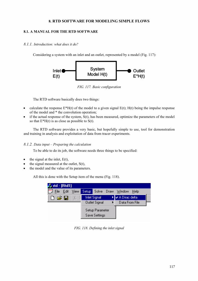
8. RTD SOFTWARE FOR MODELING SIMPLE FLOWS

8.1. A MANUAL FOR THE RTD SOFTWARE

8.1.1. Introduction: what does it do?

Considering a system with an inlet and an outlet, represented by a model (Fig. 117):

SystemModel H(t)

InletE(t)

OutletE*H(t)

SystemModel H(t)

InletE(t)

OutletE*H(t)

FIG. 117. Basic configuration

The RTD software basically does two things:

• calculate the response E*H(t) of the model to a given signal E(t); H(t) being the impulse response of the model and * the convolution operation;

• if the actual response of the system, S(t), has been measured, optimize the parameters of the model so that E*H(t) is as close as possible to S(t).

The RTD software provides a very basic, but hopefully simple to use, tool for demonstration

and training in analysis and exploitation of data from tracer experiments.

8.1.2. Data input – Preparing the calculation

To be able to do its job, the software needs three things to be specified:

• the signal at the inlet, E(t), • the signal measured at the outlet, S(t), • the model and the value of its parameters.

All this is done with the Setup item of the menu (Fig. 118).

FIG. 118. Defining the inlet signal

117

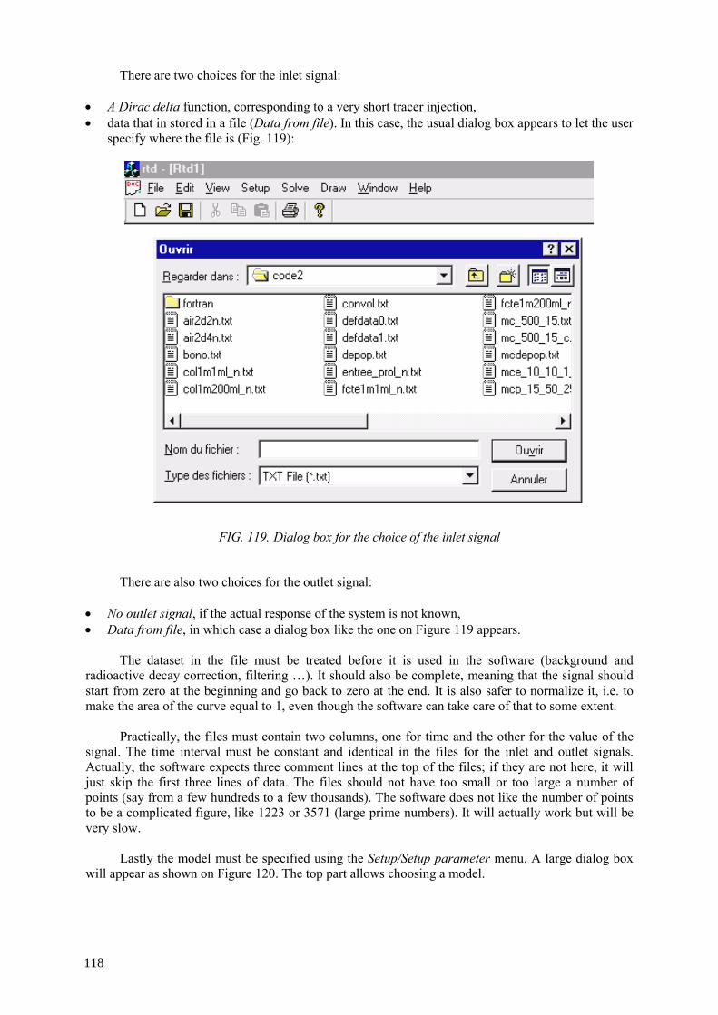
There are two choices for the inlet signal:

• A Dirac delta function, corresponding to a very short tracer injection, • data that in stored in a file (Data from file). In this case, the usual dialog box appears to let the user

specify where the file is (Fig. 119):

FIG. 119. Dialog box for the choice of the inlet signal

There are also two choices for the outlet signal:

• No outlet signal, if the actual response of the system is not known, • Data from file, in which case a dialog box like the one on Figure 119 appears.

The dataset in the file must be treated before it is used in the software (background and

radioactive decay correction, filtering …). It should also be complete, meaning that the signal should start from zero at the beginning and go back to zero at the end. It is also safer to normalize it, i.e. to make the area of the curve equal to 1, even though the software can take care of that to some extent.

Practically, the files must contain two columns, one for time and the other for the value of the

signal. The time interval must be constant and identical in the files for the inlet and outlet signals. Actually, the software expects three comment lines at the top of the files; if they are not here, it will just skip the first three lines of data. The files should not have too small or too large a number of points (say from a few hundreds to a few thousands). The software does not like the number of points to be a complicated figure, like 1223 or 3571 (large prime numbers). It will actually work but will be very slow.

Lastly the model must be specified using the Setup/Setup parameter menu. A large dialog box

will appear as shown on Figure 120. The top part allows choosing a model.

118

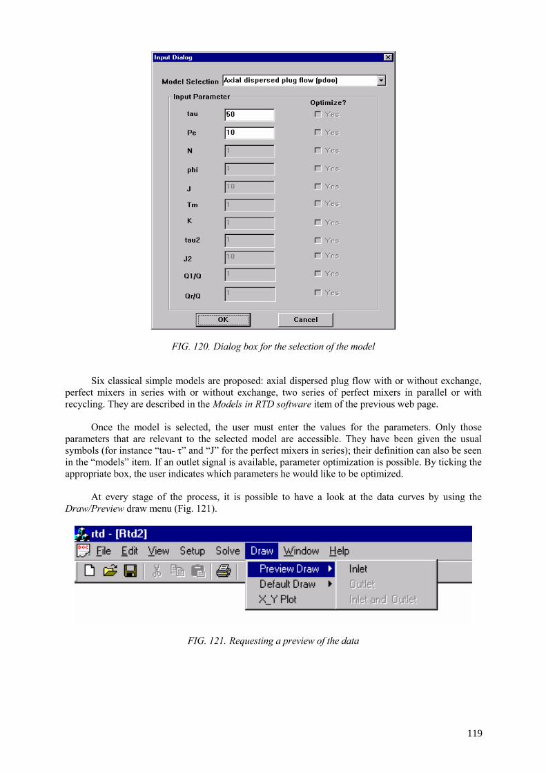
FIG. 120. Dialog box for the selection of the model

Six classical simple models are proposed: axial dispersed plug flow with or without exchange,

perfect mixers in series with or without exchange, two series of perfect mixers in parallel or with recycling. They are described in the Models in RTD software item of the previous web page.

Once the model is selected, the user must enter the values for the parameters. Only those

parameters that are relevant to the selected model are accessible. They have been given the usual symbols (for instance “tau- τ” and “J” for the perfect mixers in series); their definition can also be seen in the “models” item. If an outlet signal is available, parameter optimization is possible. By ticking the appropriate box, the user indicates which parameters he would like to be optimized.

At every stage of the process, it is possible to have a look at the data curves by using the

Draw/Preview draw menu (Fig. 121).

FIG. 121. Requesting a preview of the data

119

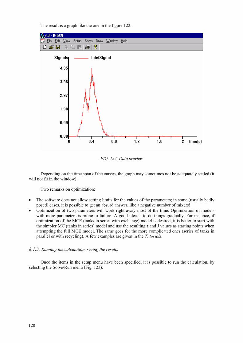
The result is a graph like the one in the figure 122.

FIG. 122. Data preview

Depending on the time span of the curves, the graph may sometimes not be adequately scaled (it

will not fit in the window). Two remarks on optimization:

• The software does not allow setting limits for the values of the parameters; in some (usually badly posed) cases, it is possible to get an absurd answer, like a negative number of mixers!

• Optimization of two parameters will work right away most of the time. Optimization of models with more parameters is prone to failure. A good idea is to do things gradually. For instance, if optimization of the MCE (tanks in series with exchange) model is desired, it is better to start with the simpler MC (tanks in series) model and use the resulting τ and J values as starting points when attempting the full MCE model. The same goes for the more complicated ones (series of tanks in parallel or with recycling). A few examples are given in the Tutorials.

8.1.3. Running the calculation, seeing the results

Once the items in the setup menu have been specified, it is possible to run the calculation, by

selecting the Solve/Run menu (Fig. 123):

120

FIG. 123. Launching the calculation

A DOS window appears very briefly if no optimization is requested, at more length otherwise. It

may be useful to know that the calculations are made using model formulation in the Laplace domain, with numerical inversion by Fast Fourier Transform. The latter is the reason why the software does not accept unequally spaced time intervals or will not work properly with an incomplete dataset.

At this stage, it is a good idea to have a look at the results by using the Draw/Default draw

menu. It is possible to see either the result of the calculation with the initial values of the parameters (Draw/Default/Unoptimised) or, if optimization has been requested, with the optimal values (Draw/Default/Optimized). The latter case is illustrated on Figure 124.

FIG. 124. Default visualisation of results

121

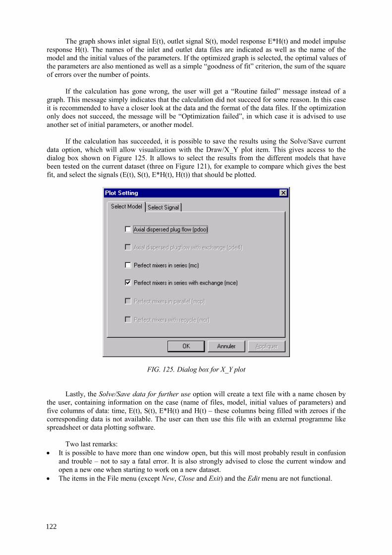
The graph shows inlet signal E(t), outlet signal S(t), model response E*H(t) and model impulse response H(t). The names of the inlet and outlet data files are indicated as well as the name of the model and the initial values of the parameters. If the optimized graph is selected, the optimal values of the parameters are also mentioned as well as a simple “goodness of fit” criterion, the sum of the square of errors over the number of points.

If the calculation has gone wrong, the user will get a “Routine failed” message instead of a

graph. This message simply indicates that the calculation did not succeed for some reason. In this case it is recommended to have a closer look at the data and the format of the data files. If the optimization only does not succeed, the message will be “Optimization failed”, in which case it is advised to use another set of initial parameters, or another model.

If the calculation has succeeded, it is possible to save the results using the Solve/Save current

data option, which will allow visualization with the Draw/X_Y plot item. This gives access to the dialog box shown on Figure 125. It allows to select the results from the different models that have been tested on the current dataset (three on Figure 121), for example to compare which gives the best fit, and select the signals (E(t), S(t), E*H(t), H(t)) that should be plotted.

FIG. 125. Dialog box for X_Y plot

Lastly, the Solve/Save data for further use option will create a text file with a name chosen by

the user, containing information on the case (name of files, model, initial values of parameters) and five columns of data: time, E(t), S(t), E*H(t) and H(t) – these columns being filled with zeroes if the corresponding data is not available. The user can then use this file with an external programme like spreadsheet or data plotting software.

Two last remarks:

• It is possible to have more than one window open, but this will most probably result in confusion and trouble – not to say a fatal error. It is also strongly advised to close the current window and open a new one when starting to work on a new dataset.

• The items in the File menu (except New, Close and Exit) and the Edit menu are not functional.

122

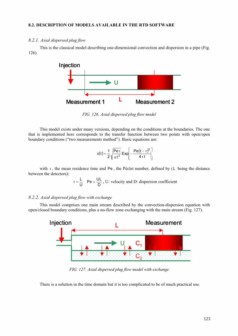
8.2. DESCRIPTION OF MODELS AVAILABLE IN THE RTD SOFTWARE

8.2.1. Axial dispersed plug flow

This is the classical model describing one-dimensional convection and dispersion in a pipe (Fig. 126).

Measurement 1 Measurement 2L

U

Injection

Measurement 1 Measurement 2L

U

Measurement 1 Measurement 2L

U

InjectionInjection

FIG. 126. Axial dispersed plug flow model

This model exists under many versions, depending on the conditions at the boundaries. The one

that is implemented here corresponds to the transfer function between two points with open/open boundary conditions (“two measurements method”). Basic equations are:

( ) ( )⎥⎥⎦

⎤

⎢⎢⎣

⎡

ττ−

−π

τ=

t4tPeExp

tPe

21tc

2

3

with τ , the mean residence time and Pe , the Péclet number, defined by (L being the distance

between the detectors):

DLUPe

UL

==τ , U: velocity and D: dispersion coefficient

8.2.2. Axial dispersed plug flow with exchange

This model comprises one main stream described by the convection-dispersion equation with open/closed boundary conditions, plus a no-flow zone exchanging with the main stream (Fig. 127).

MeasurementL

U

Injection

C1

C2

MeasurementL

U

Injection

C1

C2

FIG. 127. Axial dispersed plug flow model with exchange

There is a solution in the time domain but it is too complicated to be of much practical use.

123

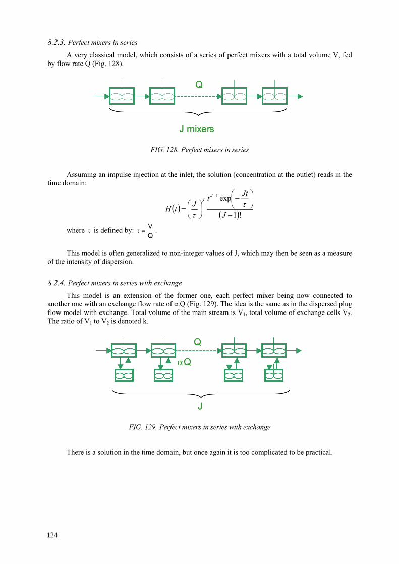
8.2.3. Perfect mixers in series

A very classical model, which consists of a series of perfect mixers with a total volume V, fed by flow rate Q (Fig. 128).

Q

J mixers

Q

J mixers

FIG. 128. Perfect mixers in series

Assuming an impulse injection at the inlet, the solution (concentration at the outlet) reads in the

time domain:

( ) ( )!1

exp1

−

⎟⎠⎞

⎜⎝⎛−

⎟⎠⎞

⎜⎝⎛=

−

J

JttJtH

JJ

ττ

where τ is defined by: QV

=τ .

This model is often generalized to non-integer values of J, which may then be seen as a measure

of the intensity of dispersion.

8.2.4. Perfect mixers in series with exchange

This model is an extension of the former one, each perfect mixer being now connected to another one with an exchange flow rate of α.Q (Fig. 129). The idea is the same as in the dispersed plug flow model with exchange. Total volume of the main stream is V1, total volume of exchange cells V2. The ratio of V1 to V2 is denoted k.

Q

J

αQ

Q

J

αQ

FIG. 129. Perfect mixers in series with exchange

There is a solution in the time domain, but once again it is too complicated to be practical.

124

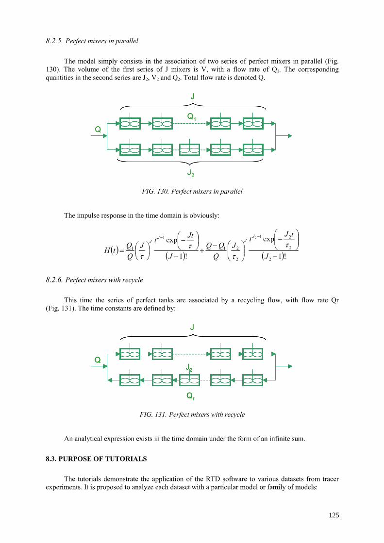
8.2.5. Perfect mixers in parallel

The model simply consists in the association of two series of perfect mixers in parallel (Fig.

130). The volume of the first series of J mixers is V, with a flow rate of Q1. The corresponding quantities in the second series are J2, V2 and Q2. Total flow rate is denoted Q.

J2

Q

Q1

J

J2

Q

Q1

J

FIG. 130. Perfect mixers in parallel

The impulse response in the time domain is obviously:

( ) ( ) ( )!1

exp

!1

exp

2

2

21

2

21

1

1

2

−

⎟⎟⎠

⎞⎜⎜⎝

⎛−

⎟⎟⎠

⎞⎜⎜⎝

⎛−+

−

⎟⎠⎞

⎜⎝⎛−

⎟⎠⎞

⎜⎝⎛=

−−

J

tJtJ

QQQ

J

JttJ

QQtH

JJ

JJ τ

ττ

τ

8.2.6. Perfect mixers with recycle

This time the series of perfect tanks are associated by a recycling flow, with flow rate Qr

(Fig. 131). The time constants are defined by:

J2

Q

Qr

J

J2

Q

Qr

J2

Q

Qr

J

FIG. 131. Perfect mixers with recycle

An analytical expression exists in the time domain under the form of an infinite sum.

8.3. PURPOSE OF TUTORIALS

The tutorials demonstrate the application of the RTD software to various datasets from tracer

experiments. It is proposed to analyze each dataset with a particular model or family of models:

125

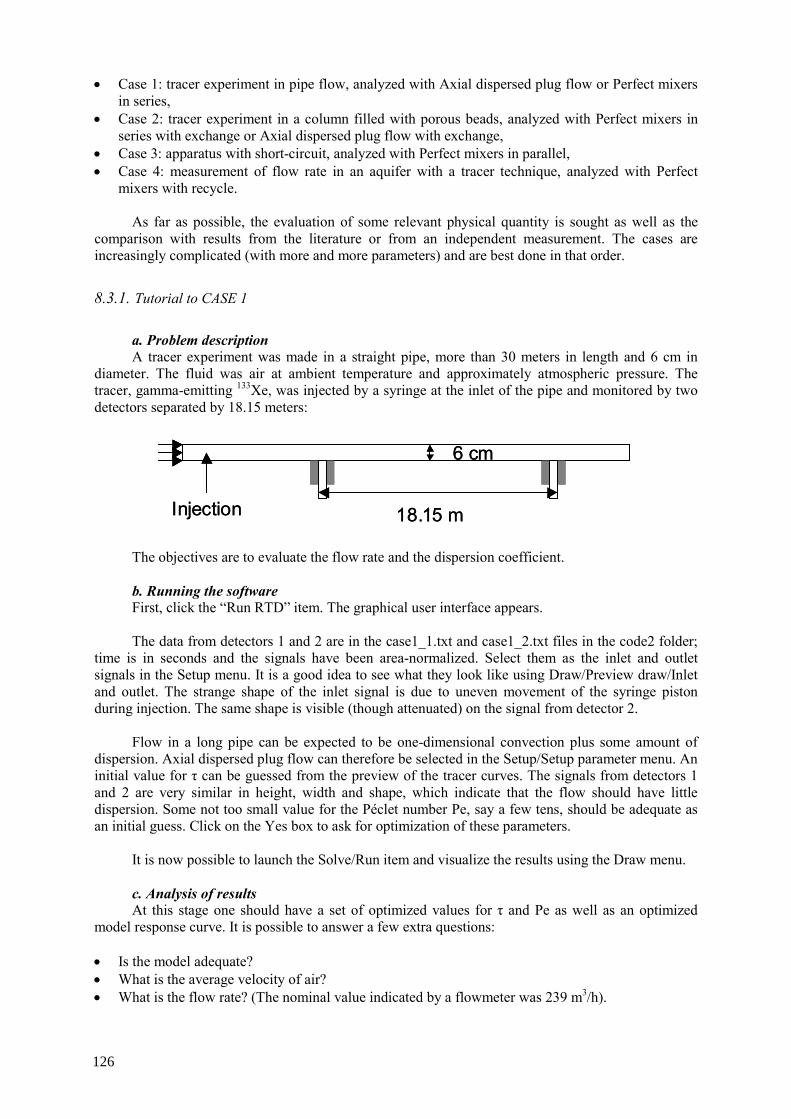
• Case 1: tracer experiment in pipe flow, analyzed with Axial dispersed plug flow or Perfect mixers in series,

• Case 2: tracer experiment in a column filled with porous beads, analyzed with Perfect mixers in series with exchange or Axial dispersed plug flow with exchange,

• Case 3: apparatus with short-circuit, analyzed with Perfect mixers in parallel, • Case 4: measurement of flow rate in an aquifer with a tracer technique, analyzed with Perfect

mixers with recycle. As far as possible, the evaluation of some relevant physical quantity is sought as well as the

comparison with results from the literature or from an independent measurement. The cases are increasingly complicated (with more and more parameters) and are best done in that order.

8.3.1. Tutorial to CASE 1

a. Problem description A tracer experiment was made in a straight pipe, more than 30 meters in length and 6 cm in

diameter. The fluid was air at ambient temperature and approximately atmospheric pressure. The tracer, gamma-emitting 133Xe, was injected by a syringe at the inlet of the pipe and monitored by two detectors separated by 18.15 meters:

18.15 m

6 cm

Injection 18.15 m

6 cm

Injection

The objectives are to evaluate the flow rate and the dispersion coefficient. b. Running the software First, click the “Run RTD” item. The graphical user interface appears. The data from detectors 1 and 2 are in the case1_1.txt and case1_2.txt files in the code2 folder;

time is in seconds and the signals have been area-normalized. Select them as the inlet and outlet signals in the Setup menu. It is a good idea to see what they look like using Draw/Preview draw/Inlet and outlet. The strange shape of the inlet signal is due to uneven movement of the syringe piston during injection. The same shape is visible (though attenuated) on the signal from detector 2.

Flow in a long pipe can be expected to be one-dimensional convection plus some amount of

dispersion. Axial dispersed plug flow can therefore be selected in the Setup/Setup parameter menu. An initial value for τ can be guessed from the preview of the tracer curves. The signals from detectors 1 and 2 are very similar in height, width and shape, which indicate that the flow should have little dispersion. Some not too small value for the Péclet number Pe, say a few tens, should be adequate as an initial guess. Click on the Yes box to ask for optimization of these parameters.

It is now possible to launch the Solve/Run item and visualize the results using the Draw menu. c. Analysis of results At this stage one should have a set of optimized values for τ and Pe as well as an optimized

model response curve. It is possible to answer a few extra questions:

• Is the model adequate? • What is the average velocity of air? • What is the flow rate? (The nominal value indicated by a flowmeter was 239 m3/h).

126

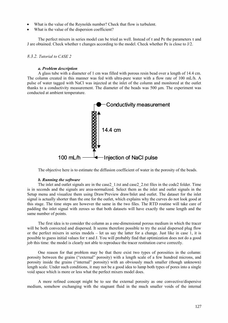
• What is the value of the Reynolds number? Check that flow is turbulent. • What is the value of the dispersion coefficient?

The perfect mixers in series model can be tried as well. Instead of τ and Pe the parameters τ and

J are obtained. Check whether τ changes according to the model. Check whether Pe is close to J/2.

8.3.2. Tutorial to CASE 2

a. Problem description A glass tube with a diameter of 1 cm was filled with porous resin bead over a length of 14.4 cm.

The column created in this manner was fed with ultra-pure water with a flow rate of 100 mL/h. A pulse of water tagged with NaCl was injected at the inlet of the column and monitored at the outlet thanks to a conductivity measurement. The diameter of the beads was 500 μm. The experiment was conducted at ambient temperature.

14.4 cm

100 mL/h

Conductivity measurement

Injection of NaCl pulse

14.4 cm

100 mL/h

Conductivity measurement

Injection of NaCl pulse The objective here is to estimate the diffusion coefficient of water in the porosity of the beads. b. Running the software The inlet and outlet signals are in the case2_1.txt and case2_2.txt files in the code2 folder. Time

is in seconds and the signals are area-normalized. Select them as the inlet and outlet signals in the Setup menu and visualize them using Draw/Preview draw/Inlet and outlet. The dataset for the inlet signal is actually shorter than the one for the outlet, which explains why the curves do not look good at this stage. The time steps are however the same in the two files. The RTD routine will take care of padding the inlet signal with zeroes so that both datasets will have exactly the same length and the same number of points.

The first idea is to consider the column as a one-dimensional porous medium in which the tracer

will be both convected and dispersed. It seems therefore possible to try the axial dispersed plug flow or the perfect mixers in series models – let us say the latter for a change. Just like in case 1, it is possible to guess initial values for τ and J. You will probably find that optimization does not do a good job this time: the model is clearly not able to reproduce the tracer restitution curve correctly.

One reason for that problem may be that there exist two types of porosities in the column:

porosity between the grains (“external” porosity) with a length scale of a few hundred microns, and porosity inside the grains (“internal” porosity) with an obviously much smaller (though unknown) length scale. Under such conditions, it may not be a good idea to lump both types of pores into a single void space which is more or less what the perfect mixers model does.

A more refined concept might be to see the external porosity as one convective/dispersive

medium, somehow exchanging with the stagnant fluid in the much smaller voids of the internal

127

porosity. In other words, the experiment could hopefully be represented with the mixers in series with exchange model.

Because the parameters are more numerous, optimizing this model can be a bit tricky. It is

suggested to take the values for τ and J optimized with the perfect mixers in series model as a starting point, along with a small value for k (say 0.1) and a value for Tm a small fraction of τ, for instance 10. If the starting point is changed, the software will either fail or give the same set of optimal values. In the latter case, the fit is almost perfect.

c. Analysis of results The result of this procedure is a set of τ, J, Tm and k values. Using our conceptual

representation of the column, it is possible to deduce the total, external and internal porosity. Exchange between the external and internal porosities is controlled by several phenomena, the

most important being often diffusion in the internal porosity. In that case, it is possible to show that the apparent diffusion coefficient of the diffusing species in the internal porosity

Compare the result with the molecular diffusion coefficient of NaCl in water (about 1.5 10-9

m2/s at 25°C). Does the difference make sense and (if so) how do you account for it?

8.3.3. Tutorial to CASE 3

a. Problem description This case deals with a heat exchanger. A tracer experiment was conducted in the “cold” circuit

of that exchanger, normally fed with water at ambient temperature. Nominal flow rate is 1.7 m3/h. The tracer was 82Br as NH4Br; it was monitored at the outlet of the exchanger only. Injection was assumed to be a very short pulse. The tracer restitution curve has two peaks, which may be interpreted as the result of a short-circuit somewhere in the exchanger. The objective is now to determine the corresponding flow rate.

b. Running the software The outlet signal is in the case3.txt file in the code2 folder. Select a Dirac delta as the inlet

function and this file as the outlet signal in the Setup menu. Visualize the data. Time is in seconds. Data is not area-normalized this time; the RTD routine will do the normalization when the Solve/Run menu is invoked.

The obvious choice for the model is perfect mixers in parallel. Examination of the curve

suggests values for the time constants of each branch (a few seconds for the short-circuit, about 200 seconds for the main flow). It also indicates the short-circuit should be a small fraction of the total flow, maybe a few percents. The shape of the curve also indicates that the J’s should not be large, say about 5. This information allows to select reasonable initial values for the parameters and to run the optimization successfully. The fit is however not excellent, perhaps because the inlet signal is not quite a Dirac function.

In the general case, this model may prove a bit tricky to optimize. It may be wise to find

parameters for the main peak first, using the perfect mixers in series, and to add the second branch only then.

c. Analysis of results

• Determine the flow rate in the short-circuit and in the main flow, • Is it possible to determine the volume of the “cold” side of the exchanger?

128

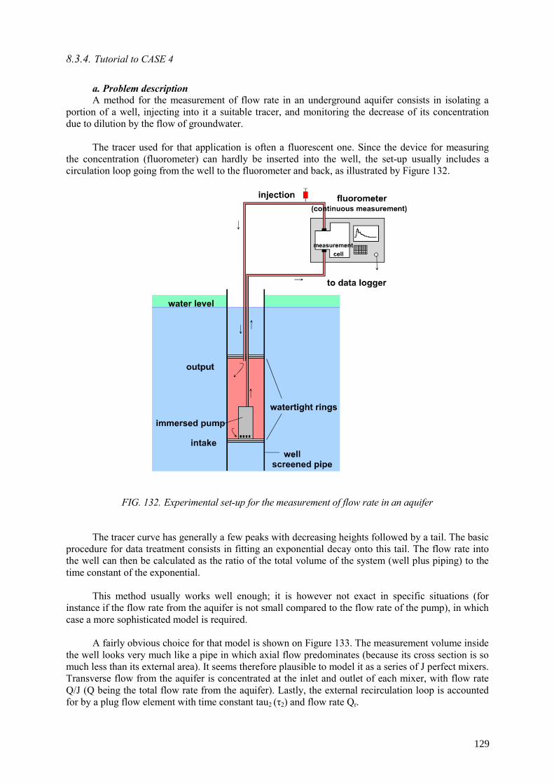
8.3.4. Tutorial to CASE 4

a. Problem description A method for the measurement of flow rate in an underground aquifer consists in isolating a

portion of a well, injecting into it a suitable tracer, and monitoring the decrease of its concentration due to dilution by the flow of groundwater.

The tracer used for that application is often a fluorescent one. Since the device for measuring

the concentration (fluorometer) can hardly be inserted into the well, the set-up usually includes a circulation loop going from the well to the fluorometer and back, as illustrated by Figure 132.

FIG. 132. Experimental set-up for the measurement of flow rate in an aquifer

The tracer curve has generally a few peaks with decreasing heights followed by a tail. The basic

procedure for data treatment consists in fitting an exponential decay onto this tail. The flow rate into the well can then be calculated as the ratio of the total volume of the system (well plus piping) to the time constant of the exponential.

This method usually works well enough; it is however not exact in specific situations (for

instance if the flow rate from the aquifer is not small compared to the flow rate of the pump), in which case a more sophisticated model is required.

A fairly obvious choice for that model is shown on Figure 133. The measurement volume inside

the well looks very much like a pipe in which axial flow predominates (because its cross section is so much less than its external area). It seems therefore plausible to model it as a series of J perfect mixers. Transverse flow from the aquifer is concentrated at the inlet and outlet of each mixer, with flow rate Q/J (Q being the total flow rate from the aquifer). Lastly, the external recirculation loop is accounted for by a plug flow element with time constant tau2 (τ2) and flow rate Qr.

129

Q/J

Qr

J

Q/J

Q/JQ/J

Q/JQ/JQ/J

Q/J

Qr tau2

Q/J

Qr

J

Q/J

Q/JQ/J

Q/JQ/JQ/J

Q/J

Qr tau2 FIG. 133. A model for the experimental set-up of fig. 132

Since the RTD software does not have this model, it may be lumped the inflow from the aquifer

at the beginning of the series of mixers and the outflow at the end, as illustrated by Figure 134. This version looks a lot like the perfect mixers with recycle in the software if the number of mixers in the recirculation branch J2 is made very large.

J2

Q

Qr

JQ

J2

Q

Qr

JQ

FIG. 134. A modified version of the model of fig. 133

b. Running the software It is proposed to test this method on data obtained in a laboratory mock-up (the “well” was

actually a plastic pipe with many branches on the sides to simulate flow from the aquifer). The interest is that Q and Qr were both precisely controlled, which allows to check the data treatment procedure. In this particular case, recycle flow rate was 0.88 L/min. The objective is to deduce “aquifer” flow rate Qr.

The outlet signal is in the case4.txt file in the code2 folder. The inlet function is supposed to be

close to a Dirac delta. Select and visualize the data (time is in minutes and the curve has been area-normalized). Select the Perfect mixers with recycle model.

The first peak comes out at 0.6 min, which should be a good starting point for τ. The interval

between two peaks being about 2 minutes, tau2 can be expected to be about 1.4 min. A “moderate” value (say less than 10) is usual for J. J2 should on the contrary be quite large. It is suggested to set it at 1000 and not to optimize it. The ratio of recycle to main flow rate is not known – the whole point being to get an estimate for it – a good initial value may be 1. The optimization should then run smoothly. One can now calculate Qr, because both Qr and Qr/Q are known, and compare with the actual value of 0.113 L/min.

130

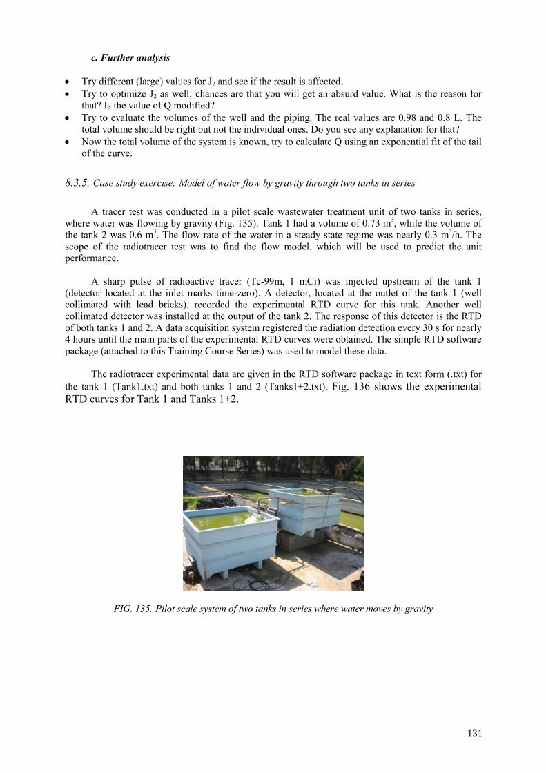
c. Further analysis

• Try different (large) values for J2 and see if the result is affected, • Try to optimize J2 as well; chances are that you will get an absurd value. What is the reason for

that? Is the value of Q modified? • Try to evaluate the volumes of the well and the piping. The real values are 0.98 and 0.8 L. The

total volume should be right but not the individual ones. Do you see any explanation for that? • Now the total volume of the system is known, try to calculate Q using an exponential fit of the tail

of the curve.

A tracer test was conducted in a pilot scale wastewater treatment unit of two tanks in series,

where water was flowing by gravity (Fig. 135). Tank 1 had a volume of 0.73 m3, while the volume of the tank 2 was 0.6 m3. The flow rate of the water in a steady state regime was nearly 0.3 m3/h. The scope of the radiotracer test was to find the flow model, which will be used to predict the unit performance.

A sharp pulse of radioactive tracer (Tc-99m, 1 mCi) was injected upstream of the tank 1

(detector located at the inlet marks time-zero). A detector, located at the outlet of the tank 1 (well collimated with lead bricks), recorded the experimental RTD curve for this tank. Another well collimated detector was installed at the output of the tank 2. The response of this detector is the RTD of both tanks 1 and 2. A data acquisition system registered the radiation detection every 30 s for nearly 4 hours until the main parts of the experimental RTD curves were obtained. The simple RTD software package (attached to this Training Course Series) was used to model these data.

The radiotracer experimental data are given in the RTD software package in text form (.txt) for

the tank 1 (Tank1.txt) and both tanks 1 and 2 (Tanks1+2.txt). Fig. 136 shows the experimental RTD curves for Tank 1 and Tanks 1+2.

FIG. 135. Pilot scale system of two tanks in series where water moves by gravity

131

8.3.5. Case study exercise: Model of water flow by gravity through two tanks in series

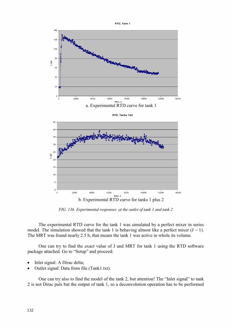
a. Experimental RTD curve for tank 1

b. Experimental RTD curve for tanks 1 plus 2

FIG. 136. Experimental responses at the outlet of tank 1 and tank 2

The experimental RTD curve for the tank 1 was simulated by a perfect mixer in series

model. The simulation showed that the tank 1 is behaving almost like a perfect mixer (J ~ 1). The MRT was found nearly 2.5 h, that means the tank 1 was active in whole its volume.

One can try to find the exact value of J and MRT for tank 1 using the RTD software

package attached. Go to “Setup” and proceed:

• Inlet signal: A Dirac delta; • Outlet signal: Data from file (Tank1.txt).

One can try also to find the model of the tank 2, but attention! The “Inlet signal” to tank

2 is not Dirac puls but the output of tank 1, so a deconvolution operation has to be performed

132

to find out the RTD of tank 2; the RTD software helps to perform the deconvolution operation. Go again to “Setup” and proceed:

• Inlet signal: Data from file (Tank1.txt) • Outlet signal: Data from file (Tanks1+2.txt).

At the end it can be found out that the tank 2 also behaviours as almost perfect mixer

(J~ 1) and the MRT of water flow is 1.5 hours (when the theoretical MRT is 2 hours). This means that tank 2 is perfect mixer in 75% of its physical volume only (25% of volume is stagnant).

9. LABORATORY WORKS

9.1. CLOSED CIRCUIT WATER FLOW RIG FOR LABORATORY RTD TESTS

9.1.1. Flow rig experimental setup

Flow rig is a laboratory set up for demonstrating radiotracer test in various conditions of flow

rate and flow models (Fig. 137). Flow rig consists of a tank of 175 L with four stirrers, a pump flowing the water inside the rig, two flow meters for measuring flow rates in two different braches, several two and three way valves for regulating the flow direction and regime, two injection points, pipes and ion exchange resin column for trapping the radiotracer after a test. Flow rate of water in the system may vary in the range of 5-15 L/min.

FIG. 137. Laboratory flow rig for exercising radiotracer tests.

Different flow patterns can be simulated using flow rig; they are presented in the fig. 138.

133

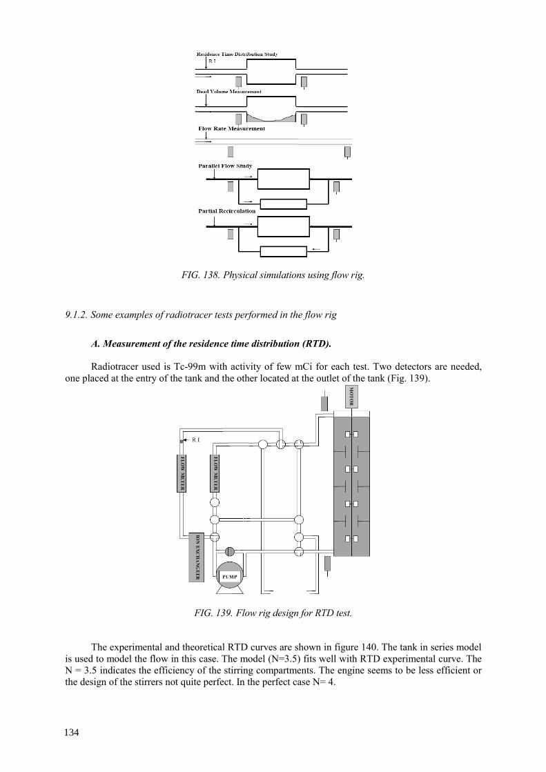
FIG. 138. Physical simulations using flow rig.

9.1.2. Some examples of radiotracer tests performed in the flow rig

A. Measurement of the residence time distribution (RTD). Radiotracer used is Tc-99m with activity of few mCi for each test. Two detectors are needed,

one placed at the entry of the tank and the other located at the outlet of the tank (Fig. 139).

FIG. 139. Flow rig design for RTD test.

The experimental and theoretical RTD curves are shown in figure 140. The tank in series model

is used to model the flow in this case. The model (N=3.5) fits well with RTD experimental curve. The N = 3.5 indicates the efficiency of the stirring compartments. The engine seems to be less efficient or the design of the stirrers not quite perfect. In the perfect case N= 4.

134

FIG. 140. The experimental RTD curve and the theoretical model fit well

The mean residence time calculated from experimental data was: t* = 740 s. The flow rate was

14 L/ min, while the tank volume 175 L. From physical parameters of tank results that the theoretical MRT is τ = V/Q = 175 L/14 L/min = 12,5 min = 750 s. This means that practically there is not created any dead volume inside the tank.

B. Dead volume measurement The same arrangement is used for dead volume measurement, but the engine rotating the stirrers

was stopped. When stirrers are not in operation there are places inside the tank when the water stays longer and exchanges slowly with the main flow moving through the tank under the pumping effect. The experimental RTD and its model show a nearly exponential decreasing curve with quite a long tail (Fig. 141).

FIG. 141. The experimental RTD curve and the model

The experimental MRT was found of t*exp= 680 s, much lower than theoretical MRT of 750 s. Thus, the dead (or stagnant volume) results: Vd = 1 – (t* exp/ τ) = 1 – 680 / 750 = 1 – 0.81 = 0.19 = 19%. The conclusion was that when the motor is stopped the dead volume created inside the tank occupies around 19 % of its total volume.

C. By-pass measurement Two detectors are located as shown in figure 142.

135

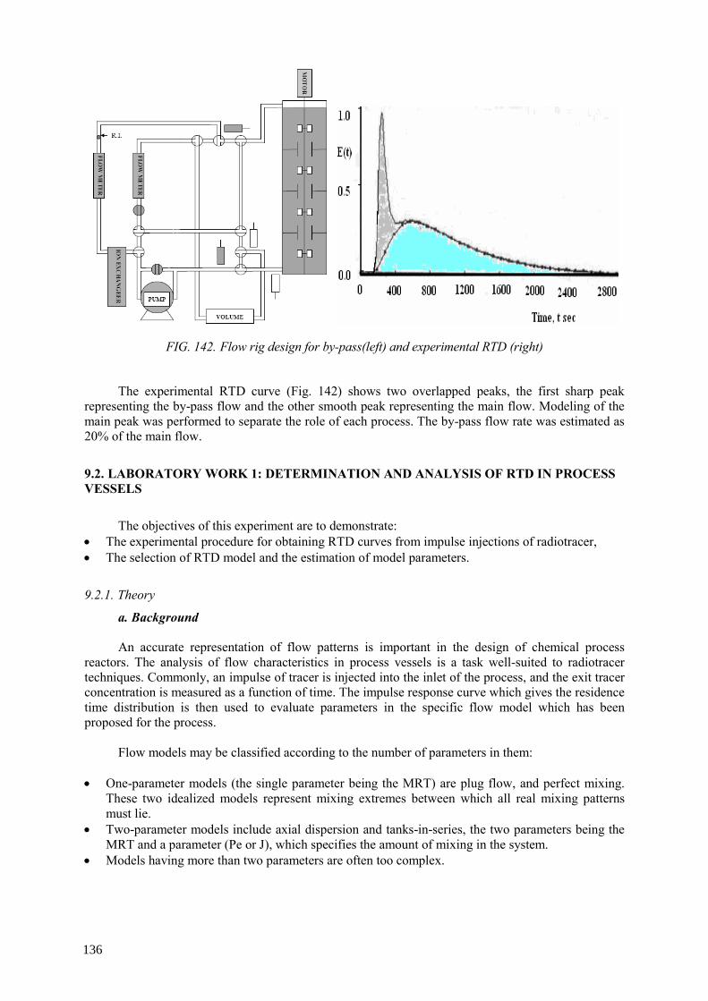
FIG. 142. Flow rig design for by-pass(left) and experimental RTD (right)

The experimental RTD curve (Fig. 142) shows two overlapped peaks, the first sharp peak

representing the by-pass flow and the other smooth peak representing the main flow. Modeling of the main peak was performed to separate the role of each process. The by-pass flow rate was estimated as 20% of the main flow.

9.2. LABORATORY WORK 1: DETERMINATION AND ANALYSIS OF RTD IN PROCESS VESSELS

The objectives of this experiment are to demonstrate:

• The experimental procedure for obtaining RTD curves from impulse injections of radiotracer, • The selection of RTD model and the estimation of model parameters.

9.2.1. Theory

a. Background An accurate representation of flow patterns is important in the design of chemical process

reactors. The analysis of flow characteristics in process vessels is a task well-suited to radiotracer techniques. Commonly, an impulse of tracer is injected into the inlet of the process, and the exit tracer concentration is measured as a function of time. The impulse response curve which gives the residence time distribution is then used to evaluate parameters in the specific flow model which has been proposed for the process.

Flow models may be classified according to the number of parameters in them:

• One-parameter models (the single parameter being the MRT) are plug flow, and perfect mixing. These two idealized models represent mixing extremes between which all real mixing patterns must lie.

• Two-parameter models include axial dispersion and tanks-in-series, the two parameters being the MRT and a parameter (Pe or J), which specifies the amount of mixing in the system.

• Models having more than two parameters are often too complex.

136

The axial dispersion model is characterizes by Peclet Number Pe. The tanks-in-series model is based on a series of J equal volume perfect mixers, each of which can be represented by the first order model. The number of tanks, J, is the mixing parameter and equals one for a perfectly mixed system and approaches infinity as the system approaches plug flow (no mixing). Although the basic concept of the tanks-in-series model requires that J be an integer, this restriction may be relaxed by replacing (J – 1)! (factorial) with the gamma function, Г (J), in the theoretical impulse response. In general, a tanks-in-series model is most appropriate for systems with relatively large amounts of mixing.

b. Techniques for estimating model parameters Two simple basic techniques available for estimating model parameters from impulse response

data are: time-domain curve fitting, and method of moments. Time-domain curve fitting is the most accurate of the three techniques, but may be difficult to

use if an analytical expression for the RTD function of the proposed model is not available. The method of moments is the simplest of the techniques, but is also the most susceptible to errors in the data. Time-domain curve fitting yields the model parameters which minimize the sum of the squares of the differences in the experimental and theoretical (model) impulse responses. For example, if Yexp(ti), i = 1, 2, .. . is the discrete experimental impulse response measured at times t1, t2, and Y(ti,parameters) is the theoretical impulse response, then

Φ= ∑ [Yexp(ti) - Y(ti, parameters)]2

is minimized by an appropriate choice of the model parameters. A nonlinear least-squares routine is commonly used to search for the optimal parameter values.

9.2.2. Part A: Determination of the residence time distribution (RTD)

The objective is to demonstrate the tracer impulse technique for determining the RTD on series of perfectly-mixed tanks of equal volume.

a. Laboratory equipment

• A system with three tanks of equal volume (about 5 L each) connected in series between the injection tee and the hold-up tank. (A tank with stirrers is used as well).

• The syringe with metal brace for injecting radioisotope solution. • A digital detector system. • A suitable aqueous solution of a short-lived radioisotope (Tc-99m). About 1/2 mL of solution with

a concentration of 1 mCi/mL is used in each injection. b. Experimental procedure The water flow through the pipe system should be adjusted between 2.5 and 5 L/min; this flow

rate will provide enough mixing within the tanks for the perfect mixing approximation to apply. The detector should be placed as near to the exit of the last tank as possible. An appropriate time interval for measuring the counting rate should be chosen and set on the digital rate meter. The system should be arranged so that the three tanks (or three stirrers) are in series.

The tracer solution should now be injected. Approximately 1/2 mL of solution containing about

1 mCi/mL should be drawn into the hypodermic syringe. The needle is inserted through the rubber septum in the injection tee and at the instant the tracer is injected, the counting apparatus is activated and the run begins. If time permits repeat the experiment for two tanks-in-series.

137

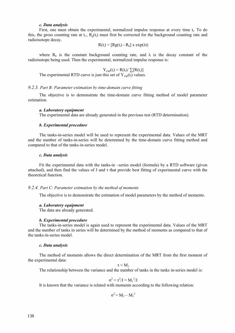
c. Data analysis First, one must obtain the experimental, normalized impulse response at every time ti. To do

this, the gross counting rate at ti., Rg(ti) must first be corrected for the background counting rate and radioisotope decay.

R(ti) = [Rg(ti) - Rb] x exp(λt) where Rb is the constant background counting rate, and λ is the decay constant of the

radioisotope being used. Then the experimental, normalized impulse response is:

Yexp(ti) = R(ti)/ ∑[R(ti)] The experimental RTD curve is just this set of Yexp(ti) values.

9.2.3. Part B: Parameter estimation by time-domain curve fitting

The objective is to demonstrate the time-domain curve fitting method of model parameter estimation.

a. Laboratory equipment The experimental data are already generated in the previous test (RTD determination). b. Experimental procedure The tanks-in-series model will be used to represent the experimental data. Values of the MRT

and the number of tanks-in-series will be determined by the time-domain curve fitting method and compared to that of the tanks-in-series model.

c. Data analysis Fit the experimental data with the tanks-in –series model (formula) by a RTD software (given

attached), and then find the values of J and τ that provide best fitting of experimental curve with the theoretical function.

9.2.4. Part C: Parameter estimation by the method of moments

The objective is to demonstrate the estimation of model parameters by the method of moments. a. Laboratory equipment The data are already generated. b. Experimental procedure The tanks-in-series model is again used to represent the experimental data. Values of the MRT

and the number of tanks in series will be determined by the method of moments as compared to that of the tanks-in-series model.

c. Data analysis The method of moments allows the direct determination of the MRT from the first moment of

the experimental data: τ = M1

The relationship between the variance and the number of tanks in the tanks in-series model is:

σ2 = τ2/J = M12/J

It is known that the variance is related with moments according to the following relation:

σ2 = M2 – M12

138

Therefore, J can be obtained from: J = M1

2/(M2 – M12)

9.3. LABORATORY WORK 2: DETECTION OF DEAD SPACE AND CHANNELLING

The primary objective of this experiment is to demonstrate the usefulness of RTD measurement

in process troubleshooting. This will be illustrated through the examination of systems in which dead space and channeling are present.

9.3.1. Theory

The analysis of a process unit for the purposes of determining dead space or channeling need

not require sophisticated mathematical treatment of the data (although it may). The purpose is not to develop a model, but simply to determine whether or not the equipment is functioning properly. An excellent example of this is determining whether or not a continuously stirred tank has sufficient agitation for the perfect mixing assumption frequently made in its design. If it does not, then one is interested in what increase in agitation is required to meet this condition; or if it does, one is interested in whether or not the power supplied can he reduced, thereby reducing operating costs while still meeting the perfect mixing requirements. A simple analysis of the shape or form of the RTD curve obtained from an impulse injection into the feed to the tank may provide all the information necessary.

Looking more closely at the continuously stirred tank, it is possible to determine what fraction

of the tank is ‘active’. The MRT, τ, of fluid entering a perfectly mixed tank is given by the equation:

τ = V/Q where V is the tank volume and Q is the volumetric flow rate. The active MRT can be determined from the analysis of the experimental RTD curve generated

by the impulse injection of a tracer : τa= [∫tR(t)dt]/[∫R(t)dt

where R(t) is the counting rate. This expression must be evaluated by numerical integration using discrete data points of R(t)

versus t, where t = 0 at the instant of injection. Of course the data taken in the experiment will not range to infinity, but for the perfectly mixed system the counting rate should return to zero after 2 or 3 MRTs. For a stirred tank in which a fraction of the total volume is dead space (no mixing in certain regions) the RTD curve it will exhibit a long tail. Defining the active volume, Va, as

Va=V- Vd

where Vd is the dead space or volume; the following is true

τa = Va/Q = (V-Vd) / Q = τ – Vd /Q and :

Vd =Q . (τ – τa) Now the fraction of the tank volume that is dead space, fd, can be calculate by the expression

fd= Vd/V = Q(τ - τa)/Q τ = 1 - τa/τ An analysis of a stirred tank system (or any system) not only allows for the determination of

whether or not there is dead space in the system, but also gives a quantitative estimate of its importance. It is obvious, however, that to be quantitative an accurate estimate of the experimental and

139

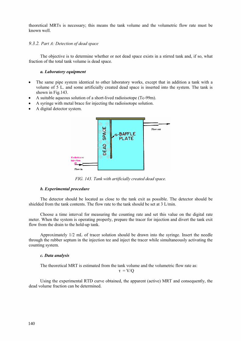
theoretical MRTs is necessary; this means the tank volume and the volumetric flow rate must be known well.

9.3.2. Part A: Detection of dead space

The objective is to determine whether or not dead space exists in a stirred tank and, if so, what

fraction of the total tank volume is dead space. a. Laboratory equipment

• The same pipe system identical to other laboratory works, except that in addition a tank with a volume of 5 L. and some artificially created dead space is inserted into the system. The tank is shown in Fig.143.

• A suitable aqueous solution of a short-lived radioisotope (Tc-99m). • A syringe with metal brace for injecting the radioisotope solution. • A digital detector system.

FIG. 143. Tank with artificially created dead space.

b. Experimental procedure The detector should be located as close to the tank exit as possible. The detector should be

shielded from the tank contents. The flow rate to the tank should be set at 3 L/min. Choose a time interval for measuring the counting rate and set this value on the digital rate

meter. When the system is operating properly, prepare the tracer for injection and divert the tank exit flow from the drain to the hold-up tank.

Approximately 1/2 mL of tracer solution should be drawn into the syringe. Insert the needle

through the rubber septum in the injection tee and inject the tracer while simultaneously activating the counting system.

c. Data analysis The theoretical MRT is estimated from the tank volume and the volumetric flow rate as:

τ = V/Q Using the experimental RTD curve obtained, the apparent (active) MRT and consequently, the

dead volume fraction can be determined.

140

9.3.3. Part B: Detection of channelling (Bypassing)

The objective is to determine whether or not channeling is occurring in a stirred tank system. a. Laboratory equipment All items are the same as in the previous Section, except that the tank added to the system in

Part A is now a tank with the entrance and exit nozzles close to one another. This tank is shown in the figure 144.

FIG. 144. Tank with artificially created channelling

b. Experimental procedure Same as in the previous Section. c. Data analysis Determine the experimental RTD curve. The curve should show two peaks, the first (normally

smaller) one is reflecting channeling of the tracer (flow) directly from the input to the output, while the second peak represents the main flow of the fluid inside the tank. The ration of two peak areas gives the percentage of the channeling effect (or by-pass transport).

9.4. LABORATORY WORK 3: RTD CURVES AND PARAMETER ESTIMATION IN COMBINED MODEL SYSTEMS

The objectives of this experiment are to demonstrate:

• that RTD curves from impulse injections into complex systems may be fit by more than one model,

• how one model may be selected as more appropriate, • what RTD curves from complex systems may look like, how models to fit these systems are

selected, and how their parameters are determined.

9.4.1. Theory

The number of real systems to which simple models, such as plug flow, perfect mixing,

dispersion or tanks-in-series can be successfully applied is limited. More complex models are usually developed on the theory that process may be considered as a number of regions, each of which may be described by a simple model such as those just listed. Further, the development of the system or process model then requires that these regions be connected properly, whether in series, in parallel, or whatever is appropriate. In addition, it may be necessary for the model, which is supposedly

141

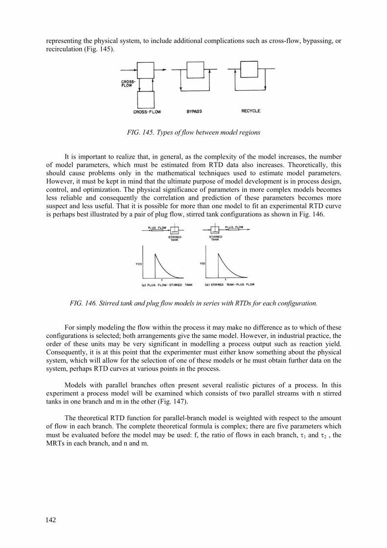
representing the physical system, to include additional complications such as cross-flow, bypassing, or recirculation (Fig. 145).

FIG. 145. Types of flow between model regions

It is important to realize that, in general, as the complexity of the model increases, the number

of model parameters, which must be estimated from RTD data also increases. Theoretically, this should cause problems only in the mathematical techniques used to estimate model parameters. However, it must be kept in mind that the ultimate purpose of model development is in process design, control, and optimization. The physical significance of parameters in more complex models becomes less reliable and consequently the correlation and prediction of these parameters becomes more suspect and less useful. That it is possible for more than one model to fit an experimental RTD curve is perhaps best illustrated by a pair of plug flow, stirred tank configurations as shown in Fig. 146.

FIG. 146. Stirred tank and plug flow models in series with RTDs for each configuration.

For simply modeling the flow within the process it may make no difference as to which of these

configurations is selected; both arrangements give the same model. However, in industrial practice, the order of these units may be very significant in modelling a process output such as reaction yield. Consequently, it is at this point that the experimenter must either know something about the physical system, which will allow for the selection of one of these models or he must obtain further data on the system, perhaps RTD curves at various points in the process.

Models with parallel branches often present several realistic pictures of a process. In this

experiment a process model will be examined which consists of two parallel streams with n stirred tanks in one branch and m in the other (Fig. 147).

The theoretical RTD function for parallel-branch model is weighted with respect to the amount

of flow in each branch. The complete theoretical formula is complex; there are five parameters which must be evaluated before the model may be used: f, the ratio of flows in each branch, τ1 and τ2 , the MRTs in each branch, and n and m.

142

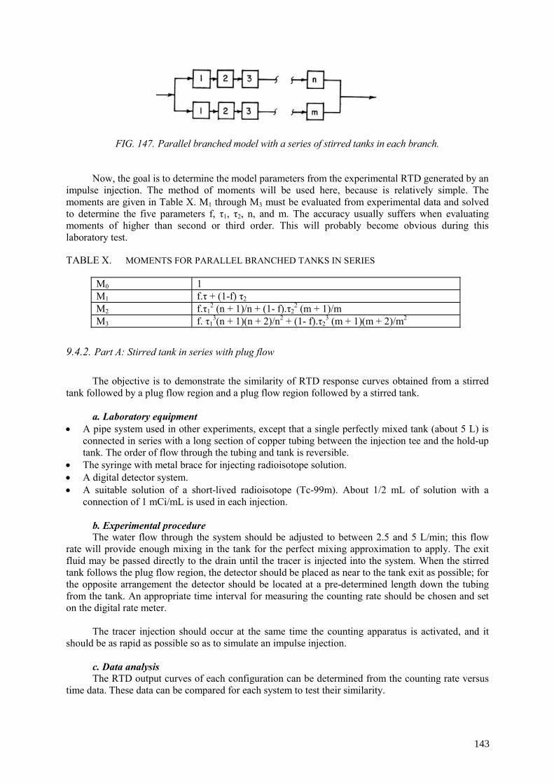
FIG. 147. Parallel branched model with a series of stirred tanks in each branch.

Now, the goal is to determine the model parameters from the experimental RTD generated by an

impulse injection. The method of moments will be used here, because is relatively simple. The moments are given in Table X. M1 through M3 must be evaluated from experimental data and solved to determine the five parameters f, τ1, τ2, n, and m. The accuracy usually suffers when evaluating moments of higher than second or third order. This will probably become obvious during this laboratory test.

TABLE X. MOMENTS FOR PARALLEL BRANCHED TANKS IN SERIES

M0 1 M1 f.τ + (1-f) τ2 M2 f.τ1

2 (n + 1)/n + (1- f).τ22 (m + 1)/m

M3 f. τ13(n + 1)(n + 2)/n2 + (1- f).τ2

3 (m + 1)(m + 2)/m2

9.4.2. Part A: Stirred tank in series with plug flow

The objective is to demonstrate the similarity of RTD response curves obtained from a stirred

tank followed by a plug flow region and a plug flow region followed by a stirred tank. a. Laboratory equipment

• A pipe system used in other experiments, except that a single perfectly mixed tank (about 5 L) is connected in series with a long section of copper tubing between the injection tee and the hold-up tank. The order of flow through the tubing and tank is reversible.

• The syringe with metal brace for injecting radioisotope solution. • A digital detector system. • A suitable solution of a short-lived radioisotope (Tc-99m). About 1/2 mL of solution with a

connection of 1 mCi/mL is used in each injection. b. Experimental procedure The water flow through the system should be adjusted to between 2.5 and 5 L/min; this flow

rate will provide enough mixing in the tank for the perfect mixing approximation to apply. The exit fluid may be passed directly to the drain until the tracer is injected into the system. When the stirred tank follows the plug flow region, the detector should be placed as near to the tank exit as possible; for the opposite arrangement the detector should be located at a pre-determined length down the tubing from the tank. An appropriate time interval for measuring the counting rate should be chosen and set on the digital rate meter.

The tracer injection should occur at the same time the counting apparatus is activated, and it

should be as rapid as possible so as to simulate an impulse injection. c. Data analysis The RTD output curves of each configuration can be determined from the counting rate versus

time data. These data can be compared for each system to test their similarity.

143

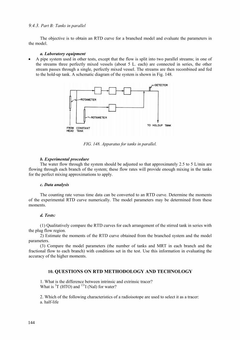
9.4.3. Part B: Tanks in parallel

The objective is to obtain an RTD curve for a branched model and evaluate the parameters in

the model. a. Laboratory equipment

• A pipe system used in other tests, except that the flow is split into two parallel streams; in one of the streams three perfectly mixed vessels (about 5 L. each) are connected in series, the other stream passes through a single, perfectly mixed vessel. The streams are then recombined and fed to the hold-up tank. A schematic diagram of the system is shown in Fig. 148.

FIG. 148. Apparatus for tanks in parallel.

b. Experimental procedure The water flow through the system should be adjusted so that approximately 2.5 to 5 L/min are

flowing through each branch of the system; these flow rates will provide enough mixing in the tanks for the perfect mixing approximations to apply.

c. Data analysis The counting rate versus time data can be converted to an RTD curve. Determine the moments

of the experimental RTD curve numerically. The model parameters may be determined from these moments.

d. Tests: (1) Qualitatively compare the RTD curves for each arrangement of the stirred tank in series with

the plug flow region. 2) Estimate the moments of the RTD curve obtained from the branched system and the model

parameters. (3) Compare the model parameters (the number of tanks and MRT in each branch and the

fractional flow to each branch) with conditions set in the test. Use this information in evaluating the accuracy of the higher moments.

10. QUESTIONS ON RTD METHODOLOGY AND TECHNOLOGY

1. What is the difference between intrinsic and extrinsic tracer? What is 3T (HTO) and 131I (NaI) for water? 2. Which of the following characteristics of a radioisotope are used to select it as a tracer: a. half-life

144

b. physico-chemical behavior c. type of energy emitted d. All of above 3. For tracing organic liquid in a processing vessel, which of the following tracer is most

suitable: - Br-82 as ammonium bromide - Br-82 as methyl bromide gas - Br-82 as paradibromo benzene 4. For in situ detection which one of the radiotracers is preferred? - beta- emitter - neutron emitter - gamma emitter - alpha- emitter 5. For field work with gamma-emitter radiotracers can be used: Geiger Muller or Scintillation

detectors? What is more efficient? (Answer: Scintillation detector is much more efficient) 6. There are several scintillation detectors for gamma rays: NaI (Tl), CsI (Tl), BGO. What is

more efficient detector, and what is more common used detector in field tracer work, why? (Answer: BGO is more efficient detector; NaI(Tl) is more common used in field because is robuster and cheaper).

7. For which radiotracers is used liquid scintillation detector? (Answer: Beta emitter: T-3, C-14,

S-35)

8. What are the radioisotope generators used in industrial applications? (Answer: Mo-Tc-99m; Sn-In-113; Cs-Ba-137).

9. What are the radiotracers for gaseous tracing? (Answer: Ar-41, Xe-133, Kr-85, Kr-79, Br-82

as methyl bromide gas). 10. How it can be prepared a radiotracer for solid phase? (Answer: Mass activation in nuclear

reactor, surface absorption of a radioactive solution) 11. What are the best radiotracers for water tracing? (Answer: T-3, NaI-131, EDTA-In113) 12. What is the best radiotracer for interwell communications in oil fields? (Answer: THO) 13. Residence time distribution (RTD) is defined as: -response of the system to an impulse input - response of the system to a steep input - response of the system to a wide tracer pulse 14. Area under a normalized RTD curve should be: - infinity - unity - ten - hundred 15. Mean residence time is: - second moment of RTD curve - first moment of RTD curve - tenth moment of RTD curve

145

16. A long tail in the measured RTD curve indicates: - stagnant volume with little exchange - plug flow - well mixed flow - none of the above 17. An ideal mixer can be represented by number of tanks in series: - N=1 - N=10 - N=100 - N=1000 18. A perfect plug flow can be represented by Peclet number: - P=1 - P=10 - P=100 - P > 200 19. The axial dispersion model is usually applicable to: - Well mixed systems - Plug flow system - Plug flow with axial dispersion - Well mixed flow with dead volume 20. RTD can be used for: - troubleshooting - validation of mathematical models - to investigate the hydrodynamic behaviour of a system - to all of the above 21. Use of stir in a tank: - enhance the mixing - reduce the mixing - both of the above 22. In the reactors or process vessels having no mixing in the direction of flow takes place, then

the flow can be characterized as: a. back mixed flow b. channeling or bypassing c. plug or piston flow d. stagnant zone 23. A radiotracer study was carried out in the White Portland Cement Factory to investigate the

RTD of raw feed materials in a rotary kiln. The raw material (80% of limestone, 15% of white clay and 5% of silica sand) mean residence time within the kiln, calculated by process engineer dividing the filled physical volume V (m3) by the feed flow rate Q (m3/s) is 40 minutes. This time is needed to ensure good quality of the end product. In order to verify this data, the radiotracer test was conducted using La-140 as tracer.

146

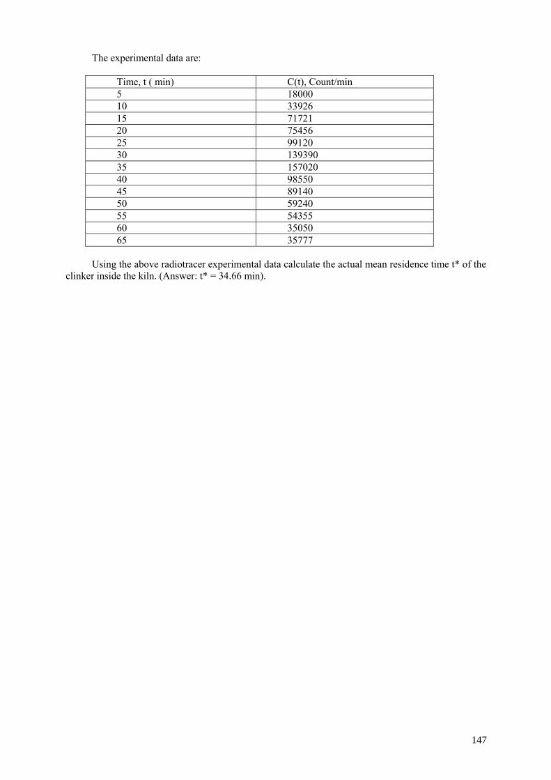
The experimental data are:

Time, t ( min) C(t), Count/min 5 18000 10 33926 15 71721 20 75456 25 99120 30 139390 35 157020 40 98550 45 89140 50 59240 55 54355 60 35050 65 35777

Using the above radiotracer experimental data calculate the actual mean residence time t* of the

clinker inside the kiln. (Answer: t* = 34.66 min).

147

BIBLIOGRAPHY

AFNOR (1983) Mesure de débit des fluides - Conduites fermées, Recueil des Normes Françaises NF X 10-131, 7. BERNE PH., BLET V. (1998) Assessment of the systemic approach using radioactive tracers and CFD, Proceedings of the 6th International conference on air distribution in rooms, Stockholm. BERNE PH., THERESKA J. Simulation of a radiotracer experiment by flow and detection-chain modelling: a first step towards better interpretation. Appl. Rad. Isotopes 60 (2004) 855-861 BERNE, PH., BLET, V., Correcting the results of radioactive tracer experiments for the effects of the detection chain (International Congress on Tracers& Tracing Methods, Nancy) (2001). BJØRNSTAD, T., “Selection of tracers for oil and gas reservoir evaluation”, Technical Research Report, IFE/KR/E-91/009 (1991) 43 pp. BORROTO J.I., DOMINGUEZ J., GRIFFITH J., FICK M., LECLERC J.P. Technetium-99m as a tracer for the liquid RTD measurement in opaque anaerobic digester: application in a sugar wastewater treatment plant. Chemical Engineering and Processing, 42 (2003) 857-865. BLET V., BERNE, PH. CHAUSSY C., PERRIN S. AND SCHWEICH D. (1999) Characterization of a packed column using radioactive tracers, Chem. Engng. Sci., 54, 91-101 BLET V., BERNE PH., FORISSIER M., LADET O., PITAULT I., SCHWEICH D. (1998) Apport de la gamma-caméra à l’étude d’un réacteur agité triphasique de laboratoire,. Proceedings of the 1st French Congress on tracers and tracer methods, Nancy. BLET, V., BERNE, Ph., TOLA, F., VITART, X., CHAUSSY, C., Recent developments in radioactive tracers methodology, Applied radiation and Isotopes, 51 (1999) 615 pp. BLET, V., BERNE, Ph., LEGOUPIL, S., VITART, X., Radioactive tracing as aid for diagnosing chemical reactors, Oil and Gas Science & Tech. 55, 2 (2000) 171. BROCHURE, TRACERCO DiagnosticsTM FCC Study, published by Tracerco, Billingham UK, 1998. BROCHURE, Process Vision Services, “Fluid tracing technology”, Tracer technology company, Brussels, Belgium, 1997. BROCHURE. Process diagnostic services Tru-Tec Services, Process Diagnostic Division, Texas, USA, 2000. CHARLTON J.S., HURST, J.A. Radioisotope techniques for problem solving in the offshore oil and gas. Petroleum technology, 1992. CHARLTON J.S. Radioisotope techniques for problem-solving in industrial process plants. Leonard Hill, Glasgow and London, 1986 CHMIELEWSKI A.G. ET AL. Application of radioisotope techniques and radiation technologies developed in Institute of Nuclear Chemistry and Technology, Warsaw, Poland. 4th Conference on Radioisotope application and radiation processing in industry, Leipzig, 19-23 September 1988., Proceedings, Vol. I, p. 143, Leipzig, 1999 CHMIELEWSKI A.G, OWCZARCZYK A., PALIGE J.; Radiotracer investigations of industrial wastewater equalizer-clarifiers, Nukleonika, Vol. 43, No. 2, 1998, p 185-194

149

CHUEINTA S. Radioisotope applications in industry. Thailand country report. AGM, IAEA/RCA Bangkok, October 2003. DANCKWERTS, P.V., Continuous flow systems, Chem. Eng. Sci. 2 (1953) 1 pp. FRIES B.A. Training the engineer for radiotracer applications in industry. In “Radiation engineering in the academic curriculum”, Proceedings of a study group meeting organized by the IAEA and held in Haifa, Israel, 26 August to 4 September 1973, Panel Proceedings Series, IAEA, 1975. FRIES B.A.. Krypton-85. A versatile tracer for industrial process applications. Int. J. Appl. Radiat. Isot. (Oct-Nov 1977). V. 28 (10-11), p. 829-832. GARDNER, R.P, ELY. JR. Radioisotope Measurement Applications in Engineering, Reinhold Publishing Corporation, New York (1967) HILLS A. Radioisotope applications for troubleshooting and optimizing industrial processes. Brochure, South Africa, 1999. INTERNATIONAL ATOMIC ENERGY AGENCY, Guidebook on Radiotracer in Industry, Technical Reports Series No. 316, IAEA, Vienna (1990). INTERNATIONAL ATOMIC ENERGY AGENCY, Radiotracer Technology as Applied to Industry, IAEA-TECDOC-1262, IAEA, Vienna, (2001). INTERNATIONAL ATOMIC ENERGY AGENCY Tracer Applications in Oil Field Investigations, Brochure, IAEA, Vienna (2003). INTERNATIONAL ATOMIC ENERGY AGENCY, Radiotracer Applications in Industry A Guidebook, Technical Reports Series No.423, IAEA, Vienna (2004). INTERNATIONAL ATOMIC ENERGY AGENCY, Integration of RTD Tracing with CFD Modelling for Industrial Process Investigations, IAEA-TECDOC-1412, IAEA, Vienna (2004). IQBAL HUSSAIN KHAN. Radioisotope applications in industry. Pakistan country report. AGM, IAEA/RCA Bangkok, October 2003. JIN, J-H. et al. Radiotracers and labelling compounds for applications in industry and environment. Report of the CM, Warsaw, Poland, 16-19 June 2004 KNOLL, G.F., Radiation detection and measurement (second edition), John Wiley & Sons, New York (1989). KOLAR, Z., THYN, J., MARTENS, W., BOELENS, G., KORVING, A., The Measurement of Gas Residence Time Distribution in a Pressurised Fluidised-Bed Combuster using 41Ar as Radiotracer, Appl. Radiat. Isot., 38 (2), (1987), 117-122. KUMAR S.B., MOSLEMIAN D., DUDUKOVIC M.P. (1997) Gas-holdup measurements in bubble columns using computed tomography. AIChe J., 43, 1414. LELINSKI D., ALLEN J., REDDEN L., WEBER A. Analysis of the residence time distribution in large flotation machines. Minerals Engineering 15 (2002) 499-505. LECLERC, J.P., DETREZ, C., BERNARD, A., SCHWEICH, D., DTS: un logiciel d’aide à l’élaboration de modèles d’écoulement dans les réacteurs Revue de l’Institut Français du Pétrole, 50 5 (1995) 641 pp.

150

LEVENSPIEL, O., Chemical reaction engineering, John Wiley & Sons, New York (1972). MAGGIO.G. Guidebook on radiotracer applications in industry. ARCAL/IAEA, Argentina, 1999. PANT H.J., THYN J., WALINJKAR O., NAVADA S.V., BHATT B.C., ZITNY C.; Radioisotope tracer study in sludge hygienisation research irradiators, IJARI, Nov. 2000. PANT, H.J., KUNDU, A., NIGAM, K.D.P., 2001. Radiotracer applications in chemical process industry. Rev. Chem Eng.17,165–252. PANT H.J., YELGOANKAR V.N. Radiotracer investigations in aniline production reactors, Applied Radiation and Isotopes 57 (2002) 319–325. PLASARI, E.; THERESKA, J., LECLERC, J.P., VILLERMAUX, J. Tracer experiments and residence-time distributions in the analysis of industrial units: case studies. Nukleonika, Vol. 44 No. 1 p.39-58, 1999, Poland. RAO, S. M. et al. (editors): “Industrial Applications of Radioisotopes and Radiation”, Wiley Eastern Limited, New Delhi (1986) SEVEL T., PEDERSEN N.H., GENDERS S. Tracing of Oil, Gas, and Water in the Oil and Gas Industry, 7th ECNDT Conference, 26-29 May (1998) SINGH G. et al. Radioisotope applications in industry. India country report, AGM, IAEA/RCA Bangkok, October 2003. THYN, J., ET AL., Analysis and diagnostics of industrial processes by radiotracers and radioisotope sealed sources, Vydavatelstvi CVUT, Praha (2000). THYN, J., RTD software analysis, Computer Manual Series n° 11, IAEA, Vienna (1996) TRACERCO, Using Radioisotope Technology to Maximise Efficiency, Petromin, 1999, p. 62-69. VAN SWAAIJ, W.P.M., CHARPENTIER, J.C., VILLERMAUX, J., Residence time distribution in the liquid phase of trickle flow in packed columns, Chem. Eng. Sc. 24 (1969) 1083 pp. VIDRINE S., HEWITT P. Radioisotope Technology -Benefits & Limitations in Troubleshooting Packed Beds in Vacuum Distillation. Presented in the Distillation Symposium of the 2005 Spring AIChE Meeting Atlanta, Ga. April 10 through 13, 2005. VILLERMAUX, J., Génie de la réaction chimique, Tec. et Doc. Lavoisier, Paris (1993). WALTAR A.E. Nuclear technology’s numerous uses. Atoms for peace: Fifty years latter. Issues in Science and Technology, 2004, p. 48-54. ZEMEL, B.: “Tracers in the Oil Field”, Elsevier Science, Amsterdam (1995) ZHANG PEIXIN. Radioisotope applications in industry. China country report. AGM, IAEA/RCA Bangkok, October 2003.

151

BIBLIOGRAPHY ON RADIATION PROTECTION AND SAFETY INTERNATIONAL ATOMIC ENERGY AGENCY, Radiation Protection and the Safety of Radiation Sources, Safety Series No.120, IAEA, Vienna (1996). INTERNATIONAL ATOMIC ENERGY AGENCY, International Basic Safety Standards for Protection against Ionizing Radiation and for the Safety of Radiation Sources, Safety Series No.115, Vienna (1996). INTERNATIONAL ATOMIC ENERGY AGENCY, Occupational Radiation Protection, IAEA Safety Standards Series No. RS-G-1-.1, Vienna (1999). INTERNATIONAL ATOMIC ENERGY AGENCY, Training in Radiation Protection and the Safe use of Radiation Sources, Safety Reports Series No. 20, IAEA, Vienna (2001). INTERNATIONAL ATOMIC ENERGY AGENCY, Legal and Governmental Infrastructure for Nuclear, Radiation, Radioactive Waste and Transport Safety, IAEA Safety Standards Series No. GS-R-1, IAEA, Vienna (2000). INTERNATIONAL ATOMIC ENERGY AGENCY, Safety Assessment Plans for Authorization and Inspection of Radiation Sources, IAEA-TECDOC-1113, IAEA, Vienna (1999). INTERNATIONAL ATOMIC ENERGY AGENCY, Regulations for the Safe Transport of Radioactive Material, IAEA Safety Standards Series No. TS-R-1 (ST-1, Rev.), IAEA, Vienna (2000). INTERNATIONAL ATOMIC ENERGY AGENCY, Preparedness and Response for a Nuclear or Radiological Emergency, IAEA Safety Standards Series, No. GS-R-2, IAEA, Vienna (2002). INTERNATIONAL ATOMIC ENERGY AGENCY, Method For the Development of Emergency Response Preparedness for Nuclear and Radiological Accidents, IAEA-TECDOC-953, IAEA, Vienna (1997).

152

CONTRIBUTORS TO DRAFTING AND REVIEW

Berne, Ph. DTEN/SAT, CEA/Grenoble, France

Bjornstad, T. Institute for Energy Technology (IFE), Reservoir and Exploration Technology, Kjeller, Norway

Brisset, P. DIMRI, CEA/Saclay, France

Charlton, S. Johnson Matthey PLC, Oatley, Australia

Chmielewski, A. Department of Nuclear Methods of Process Engineering, Institute of Nuclear Chemistry and Technology, Warsaw, Poland

Genders, S. FORCE Technology, Denmark

Griffith, J.M. Instituto Cubano de Investigaciones Azucareras (ICINAZ), Departamento de Tecnicas Nucleares, La Habana, Cuba

Hills, A. Isotope Production Centre, NECSA, Pretoria, South Africa

Jin, J.H. International Atomic Energy Agency, NAPC, Industrial Applications and Chemistry Section, Vienna, Austria

Jung S.H. Korea Atomic Energy Research Institute (KAERI),

Khan, I. H. Pakistan Institute of Nuclear Science and Technology (PINSTECH),

Radiation and Isotope Applications Division (RIAD), Islamabad, Pakistan

Maggio, G. NOLDOR S.R.L. , Buenos Aires, Argentina

Martins Moreira, R. Centro de Desenvolvimiento da Tecnologia Nuclear (CDTN), Belo Horizonte, Minas Gerais, Brazil

Pant, H. J. Bhabha Atomic Research Centre, Mumbai , India

Thereska, J. Consultant and expert, Tirana, Albania

Zhang, P. Industrial Application of Isotopes, China Institute of Atomic Energy (CIAE), Beijing, China

153

Daejon, Republic of Korea

I S S N 1 0 1 8 – 5 5 1 8