Article

Supersymmetric Partners of the One-dimensional InfiniteSquare Well Hamiltonian

M. Gadella 1 , J. Hernández-Muñoz 2 , L.M. Nieto 1* and C. San Millán 1

Citation: Gadella, M.;

Hernández-Muñoz, J.; Nieto, L.M.;

San Millán, C. Supersymmetric

Partners of the One-dimensional

Infinite Square Well Hamiltonian.

Preprints 2021, 1, 0.

https://doi.org/

Received:

Accepted:

Published:

Publisher’s Note: MDPI stays neu-

tral with regard to jurisdictional

claims in published maps and insti-

tutional affiliations.

1 Departamento de Física Teórica, Atómica y Óptica and IMUVA, Universidad de Valladolid, 47011Valladolid, Spain; manuelgadella1@gmail.com (M.G.); carloskoxax@gmail.com (C.SM.)

2 Departamento de Física Teórica de la Materia Condensada, IFIMAC Condensed Matter Physics Center,Universidad Autónoma de Madrid, Madrid 28049, Spain; josehermu93@gmail.com

* Correspondence: luismiguel.nieto.calzada@uva.es; Tel.: +34-983-423754

Abstract: We find supersymmetric partners of a family of self-adjoint operators which are self-1

adjoint extensions of the differential operator−d2/dx2 on L2[−a, a], a > 0, i.e., the one dimensional2

infinite square well. First of all, we classify these self-adjoint extensions in terms of several choices3

of the parameters determining each of the extensions. There are essentially two big groups of4

extensions. In one, the ground state has energy strictly positive. On the other, either the ground5

state has zero or negative energy. In the present paper, we show that each of the extensions6

belonging to the first group (energy of ground state strictly positive) has an infinite sequence7

of supersymmetric partners, such that the `-th order partner differs in one energy level from8

both, the (` − 1)-th and the (` + 1)-th order partners. In general, the eigenvalues for each of9

the self-adjoint extensions of −d2/dx2 come from a transcendental equation and are all infinite.10

For the case under our study, we determine the eigenvalues, which are also infinite, and their11

respective eigenfunctions for all of its `-th supersymmetric partners of each extension.12

Keywords: Supersymmetric quantum mechanics; self-adjoint extensions; infinite square well;13

contact potentials.14

1. Introduction

The study of one dimensional models in quantum mechanics is useful in order to a better understanding of theproperties of quantum systems. In particular, the construction of supersymmetric (SUSY) partners of given potentialsallow for an analysis of one dimensional Hamiltonians that often keep similarities with the original ones. Many studieshave been done in this field and a brief account of references [1–14] only covers a small part of all previous work.

In the present paper, we intend to investigate the properties of the SUSY partners of the self-adjoint determinationsof the operator −d2/dx2 on L2[−a, a], a > 0 and finite, with appropriate boundary conditions at the points −a and a.Note that this problem is closely related to the problem of the definition of the “free” Hamiltonian on the one dimensionalinfinite square well potential.

The analysis of these self-adjoint extension has been done in [15]. The task of computing the SUSY partners of all theself-adjoint determinations (also called extensions) of −d2/dx2 on L2[−a, a], their spectra and their wave functions is nottrivial, although can be carried out systematically.

Although the idea of self-adjoint extensions of symmetric (or Hermitian) operators on (infinite dimensional) Hilbertspaces is not yet very popular among physicists, it is possible to find recent papers on the topic [16–24]. Standard quantummechanics textbooks refer to the one dimensional infinite square well potential or the harmonic oscillator as if they weredescribed by a unique self-adjoint Hamiltonian, which produces a neatly calculable spectrum. The mathematical realityis much more complex and may give many more possibilities for the study of quantum mechanics systems. Let us brieflyaddress to this problem, for which a more thoroughly presentation can be found in mathematical textbooks [25] as wellas papers addressed to the Physics community [15].

Concerning terminology, an operator, A, on a infinitely dimensional separable Hilbert space1 H is symmetric,or equivalently Hermitian, if for any pair of vectors ϕ, ψ ∈ D(A), where D(A) is the domain of A, which must be

1 The Hilbert space must be infinite dimensional, since otherwise all operators are continuous and defined on the whole space. In such a case, thisargumentation does not make sense. A separable Hilbert space is one with a countable orthonormal basis, which is always the case in ordinaryquantum mechanics.

2 of 17

densely defined, one has that 〈Aϕ|ψ〉 = 〈ϕ|Aψ〉, where 〈−|−〉 denotes the scalar product on H. This means that theadjoint, A†, of A extends A, A ≺ A† (i.e., D(A) ⊂ D(A†) and Aψ = A†ψ, for all ψ ∈ D(A)). The deficiency indicesare n± := dim Ran(A† ± iI), where Ran(B) is the range (image space) of the operator B and I is the identity operator.A symmetric (or Hermitian) operator has self adjoint determinations (or extensions) if and only if n+ = n− [25]. Ifn+ = n− = 0, this extension is unique. On the other hand, if n+ = n− 6= 0, the number of extensions is infinite and, inthe case of Hilbert spaces of functions, they usually can be determined by some matching or boundary conditions thatthe functions in the domain of the extensions should fulfil at some points [15,25–27].

Self-adjoint determinations of the operator −d2/dx2 defined on functions supported whatever interval, K, in thereal line R are used to define the so call contact potentials [26,28–31]. These are perturbations of the “free operator”H0 = −d2/dx2, which are supported on a single point x0 ∈ K. Typical examples of contact potentials are the Dirac deltaδ(x− x0) or its derivative δ′(x− x0), which define Hamiltonians of the type H0 + δ(x− x0) or H0 + δ′(x− x0) as welldefined self-adjoint operators on the Hilbert space L2(K) [27]. These types of perturbations may serve as a good andtractable approximation for a very localized spatial perturbation and are defined via matching conditions that mustsatisfy the functions on the domain of the operator at x0. Concerning the operator −d2/dx2 on L2[−a, a], some relationshave been found among the boundary conditions at the borders −a and a and matching conditions defining a δ or δ′

perturbation at the origin [32,33].A comment is of relevance here. Let us consider the subspace, D0, of all twice differentiable square integrable

functions, ϕ(x), in the interval [−a, a], with second derivative in L2[−a, a], verifying the boundary conditions ϕ(−a) =ϕ(a) = ϕ′(−a) = ϕ′(a) = 0, and a differential operator of the form

D = − d2

dx2 + p1(x)d

dx+ p2(x), (1)

where p1(x) and p2(x) are continuous real functions (with p1(x) differentiable) on [−a, a]. Then D is Hermitian on D0with deficiency indices (2,2). It has been proven in [34] (vol. 2, p. 90) that all self-adjoint extensions of D have purelydiscrete spectrum. This is precisely the case of all the self-adjoint determinations of −d2/dx2 under our study [15].These self-adjoint extensions are characterized by a set of fourth real parameters, so that one particular choice of theseparameters gives a unique self-adjoint determination of −d2/dx2 on L2[−a, a] and vice-versa. Although this is much lessknown, a similar situation emerges in the study of the one dimensional harmonic oscillator [35].

The present article intends in the first place, complete as far as possible, the classification of the self-adjoint extensionsof −d2/dx2 on L2[−a, a] given by [15]. Once this task has been done, we intend to obtain the whole chain of SUSYpartners of each of the self-adjoint extensions, using standard methods already developed in the theory [1]. This kindof supersymmetry intends to construct a series of potentials (in our case one-dimensional), with an energy spectrumclosely related and that can be obtained from the spectrum of the original potential. Thus, being given one of our originalself-adjoint extensions and being known the solution of the spectral problem, we should be able to obtain an infinitesequence of Hamiltonians such that their spectra coincides with the spectra of the previous one except for one eigenvalue,and hence from the original one except for a finite number of energy levels. We must add that all self-adjoint extensionsof −d2/dx2 on L2[−a, a] have a purely discreet spectrum with an infinite number of energy levels.

The ground state for each of these extensions, either has a strictly positive, zero or negative energy. Obviously, in thelatter case, this fact come from extensions which are not positive definite. This is somehow paradoxical, due to the formof the original operator, which is −d2/dx2. This paradox is solved in [15]. For those extensions with ground state withstrictly positive energy, we have constructed the whole sequence of its SUSY partners and given the eigenvalues andeigenfunctions for these partners. As mentioned earlier, the set of eigenvalues for each partner comes from the set ofeigenvalues of the extension from which we construct the sequence of partners.

The general formalism can also be applied to obtain a sequence of Hamiltonians when the ground state of theoriginal self-adjoint extension of −d2/dx2 on L2[−a, a] has zero or negative energy. In this case, partner Hamiltoniansmay be very different from the original one in the sense that they may have a finite number of eigenvalues or simply noeigenvalues. This is due to the presence of nodes in the wave function of the ground state. Nevertheless, these partnersmay be obtained and classified, although this discussion is left for a next publication.

This paper is organized as follows: In Section 2 we reformulate the classification given by [15] of the self-adjointextensions of −d2/dx2 on L2[−a, a]. In 3, we classify these extensions in terms of some other sets of parameters, notconsidered in [15]. In 4, we construct the first SUSY partners for those extensions with positive ground level energyand give the precise form of its eigenfunctions. In 5, we give the complete sequence of SUSY partners for each of theseextensions. We close this article with a Conclusions Section and an Appendix in which we show what the correct form forthe wave functions for the energy levels should be.

3 of 17

2. Self-adjoint extensions: Determination of their eigenvalues

Let us go back to the differential operator H0 := −d2/dx2 defined on L2[−a, a], a > 0 and with domain D0 as above,just before (1). On D0, H0 is symmetric (Hermitian) with deficiency indices (2, 2) [15]. According to the von-Neumanntheorem [25], H0 admits an infinite number of self-adjoint extensions labeled by four real parameters.

The adjoint operator H†0 acts as −d2/dx2 on the functions of its domain (see [36,37] for a definition of the domain of

the adjoint of a given densely defined operator and its properties). If φ is a function of such domain, we get integratingby parts: ⟨

− d2

dx2 φ, φ

⟩= B(φ, φ) +

⟨φ,− d2

dx2 φ

⟩, (2)

where 〈−,−〉 denotes the scalar product on L2[−a, a] and

B(φ, φ) = φ′(a)φ∗(a)− φ(a)φ′∗(a)− φ′(−a)φ∗(−a) + φ(−a)φ′∗(−a), (3)

the prime being the derivative with respect to the variable x and the asterisk meaning complex conjugate. The self-adjointextensions of H0 are equal to −d2/dx2 as an operator acting on the subdomains of the domain of H†

0 of functions withB(φ, φ) = 0. This happens if and only if there exists a 2× 2 unitary matrix U such that (see [15] and references quotedtherein): 2aφ′(−a)− iφ(−a)

2aφ′(a) + iφ(a)

= U

2aφ′(−a) + iφ(−a)

2aφ′(a)− iφ(a)

. (4)

The set of self-adjoint extensions of H0 is in one to one correspondence with the set of 2× 2 unitary operators U. Thus,each of these extensions will be labeled by its corresponding operator as Hα. Since there is a set of four real independentparameters that characterize the set of operators U, then, the set of self-adjoint extensions of Hα is also characterized bythe same parameters [15]. Each of the operators U has the following form [15]:

U = eiψ

m0 − im3 −m2 − im1

m2 − im1 m0 + im3

. (5)

Here, ψ and mi, i = 0, 1, 2, 3 are real parameters so that ψ ∈ [0, π] and m20 + m2

1 + m22 + m2

3 = 1, which means that onlyfour parameters are independent [15]. The latter relation is a consequence of unitarity: the modulus of the determinant ofU must be a number of modulus one.

There are some of these extensions with a clear physical interest, which does not mean that the others are irrelevantfrom the physics point of view. In [15], the authors distinguish three categories of extensions:

i.) Those which preserve time reversal;ii.) Those which preserve parity;iii.) Those preserving positivity.

Apart from these three categories, there are some other extensions. The reason why the authors of [15] single out thoseextension that preserve positivity is due to the existence of extensions with negative energies. In fact, as proven in [34](Theorem 16, vol 2, page 44), Hα may have one (which may be doubly degenerate) or two (with no degeneration) negativeenergy states. All other extensions have non-negative eigenvalues and are called positivity preserving. Only three of thispositivity preserving extensions with special simplicity are discussed in [15]. We want to determine the energy levels inthis situation.

In order to obtain the energy levels for a specific self-adjoint extension, Hα, of H0 = −d2/dx2 on L2[−a, a], wehave to solve the Schrödinger equation and impose on its solutions the boundary conditions that characterize theextension. These boundary conditions are given by the (4) and (6). However as stated in [15], the determination ofwhich operators U satisfy the positivity condition as stated before involves tedious considerations. To circumvent thisdifficulty, let us consider the general solution of the time independent Scrödinger equation −d2φ(x)/dx2 = Eφ(x), withE = s2/(2a)2 ≥ 0, where 2a is the infinite square well width2. This general solution is,

φ(x) = A cos( sx

2a

)+ B sin

( sx2a

). (6)

2 Although the energy is given, in our notation, by h̄2E/2m, we are calling “energy” the quantity represented by E.

4 of 17

Here, A and B have to be fixed with two conditions: (i) φ(x) should be normalized in L2[−a, a] and (ii) φ(x) should fulfillthe boundary conditions (4)–(5) so that E ≥ 0. Let us use (6) in relation (4) giving the general matching conditions, so asto obtain the following homogeneous linear system:(

L(s)−UM(s))(A

B

)= N (s)

(AB

)= 0 , (7)

where

L(s) =(

s sin s2 − i cos s

2 s cos s2 + i sin s

2

−s sin s2 + i cos s

2 s cos s2 + i sin s

2

), M(s) =

(s sin s

2 + i cos s2 s cos s

2 − i sin s2

−s sin( s2 − i cos s

2 s cos s2 i sin s

2

). (8)

The eigenvalues λ±(s) of the matrix N (s) are given by

λ±(s) =Tr(N (s))

2±

√(Tr(N (s))

2

)2

− det(N (s)) (9)

The trace and the determinant of N (s) can be easily calculated and are, respectively:

Tr(N (s)) = e−12 i(s−2ψ)

(−m3(s + 1) + im2eis(s− 1)

), (10)

anddet(N (s)) = −4ieiψ

[(m0 + cos ψ) sin s + 2s(m1 − cos s sin ψ)− s2(m0 − cos ψ) sin s

]. (11)

To begin with, let us remark that in order to have non-trivial solutions of (7) we must have

det(N (s)) = 0. (12)

Then, the set of eigenvalues of N (s) is given by Tr(N (s)) and 0, as may be immediately seen from (9). The condition(12) gives a relation between the values of the energy, determined by the real parameter s, since E = s2/(2a)2, and theparameters ψ, m0 and m1, as in (5). In consequence, the energy levels depend on the values of these three parameters only.From (11) -(12) , we obtain the following two transcendental equations (one with plus sign and the other with minussign):

s sin s =m1 − cos s sin ψ

m0 − cos ψ±

√(m1 − cos s sin ψ

m0 − cos ψ

)2+

m0 + cos ψ

m0 − cos ψsin2 s . (13)

This form of the transcendental equations is quite interesting, since it will serve for an efficient estimation of the energylevels when these values cannot be exactly calculated. Otherwise, they permit to obtain exact solutions whenever theyexists. Let us summarize now three of the results provided by [15], which we will need later on:

• The eigenvector (A, B) of N (s) with 0 eigenvalue is given by

A =[i + eiψ(im0 + m1 − im2 + m3)

]sin

s2+ s[1 + eiψ(m0 + im1 + m2 + im3)

]cos

s2

, (14)

B = s[−1 + eiψ(m0 + im1 + m2 − im3)

]sin

s2+[i + eiψ(im0 −m1 + im2 + m3)

]cos

s2

. (15)

We see that the eigenvector depends on all the parameters (m0, m1, m2, m3, ψ).• The extensions preserving time reversal invariance, are given by

m2 = 0 . (16)

• The parity preserving extensions of H0 are those for which the eigenfunctions φ(x) verify :

|φ(x)|2 = |φ(−x)|2 =⇒ |φ(a)|2 = |φ(−a)|2 . (17)

5 of 17

2.1. Parity preserving extensions of H0

We are interested now in getting more information on the parity preserving extensions of H0. Then, if we use (6) in(17) we obtain that Re(A B∗) sin s = 0. Hence, either

sin s = 0 or Re(A B∗) = 0. (18)

Taking into account the values of (A, B) given in (14)–(15) and also the fact that det(N (s)) = 0, the second equation of(18) implies that either m3 = 0 or

(m3 + sin ψ) sin s + 2s(m2 + cos s cos ψ) + s2(sin ψ−m3) sin s = 0. (19)

Solving this equation, as if it were a quadratic equation on s, gives a pair of transcendental equations which closely resembleto equation (13). Thus, the complete set of solutions of (18) are

m3 = 0 , (20a)

sin s = 0 , (20b)

s sin s =m2 + cos s cos ψ

m3 − sin ψ±

√(m2 + cos s cos ψ

m3 − sin ψ

)2+

m3 + sin ψ

m3 − sin ψsin2 s . (20c)

Hence, when the parity is preserved, equation (13) holds. This happens for three different situations given by formulas(20a)–(20c). These formulas, plus (13), which derives from such a general principle as det(N (s)) = 0, should give theenergy levels for the infinite square well with parity preserving self-adjoint extensions, Hα, of H0.

Equation (20a) does not provide any extra information, (13) being the only relation which gives information on theenergy spectrum. This parity preserving condition m3 = 0 has been already used in [15], although in this paper relations(20b) and (20c) are not mentioned.

Equation (20b) obviously gives an energy spectrum of the parity preserving extensions that coincides to the spectrumgiven by texts in Quantum Mechanics for the extension with domain given by functions with φ(−a) = φ(a) = 0.Henceforth, we shall call this extension as the textbook extension.

Finally, (20c) gives the energy levels for other parity preserving extensions in terms of the three parameters(ψ, m2, m3).

In consequence, we have eight different situations for those extension having a non-negative spectrum, includingthose with time reversal and parity invariance, as shown in the Table 1. In next section we will analyze some of thesesituations.

Generic spectrum: (13)

Time reversal invariance: (13) and (16), or m2 = 0

Parity preserving:

(13) and (20a) m2 = 0m2 6= 0

(13) and (20b) m2 = 0m2 6= 0

(13) and (20c) m2 = 0m2 6= 0

Table 1: List on how to obtain the possible spectra as a function of the conserved properties.

3. Spectrum of the free particle on a finite interval

One of the goals of our study is to solve the eigenvalue problem for all the self-adjoint extensions, Hα, of the operatorH0 = −d2/dx2 on L2[−a, a], which from the point of view of the physicists is the infinite square well with width 2a. Aswe have already seen, there are only a few of these extensions for which we may obtain an exact solution, including thetextbook extension. For most of these extensions the energy levels are solutions of a transcendental equation and, therefore,no explicit solutions of the eigenvalue problem for these extensions can be given.

6 of 17

3.1. The angular representation of the self-adjoint extensions of H0

Due to the relation between the parameters mi, given by

m20 + m2

1 + m22 + m2

3 = 1, (21)

a new parametric representation of the self-adjoint extensions, Hα, of H0 = −d2/dx2 on L2[−a, a] in terms of angularvariables only is possible. Apart from the variable ψ, which is already angular, so that we keep it untouched, we havethree other angular variables, θi, i = 0, 1, 2, defined by means of the following relations:

m0 = cos θ1 cos θ0, m1 = cos θ1 sin θ0, m2 = sin θ1 cos θ2, m3 = sin θ1 sin θ2. (22)

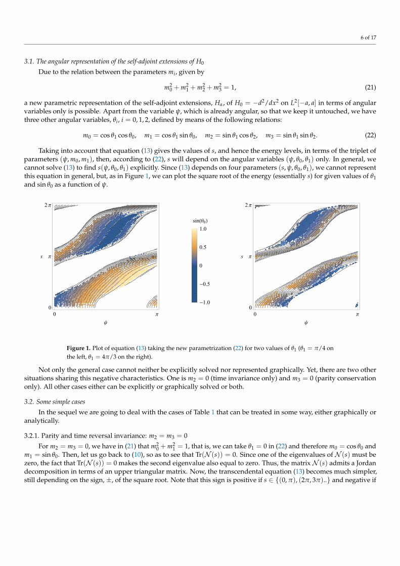
Taking into account that equation (13) gives the values of s, and hence the energy levels, in terms of the triplet ofparameters (ψ, m0, m1), then, according to (22), s will depend on the angular variables (ψ, θ0, θ1) only. In general, wecannot solve (13) to find s(ψ, θ0, θ1) explicitly. Since (13) depends on four parameters (s, ψ, θ0, θ1), we cannot representthis equation in general, but, as in Figure 1, we can plot the square root of the energy (essentially s) for given values of θ1and sin θ0 as a function of ψ.

0 π0

π

2 π

ψ

s

sin(θ0)

-1.0

-0.5

0

0.5

1.0

0 π0

π

2 π

ψ

s

Figure 1. Plot of equation (13) taking the new parametrization (22) for two values of θ1 (θ1 = π/4 onthe left, θ1 = 4π/3 on the right).

Not only the general case cannot neither be explicitly solved nor represented graphically. Yet, there are two othersituations sharing this negative characteristics. One is m2 = 0 (time invariance only) and m3 = 0 (parity conservationonly). All other cases either can be explicitly or graphically solved or both.

3.2. Some simple cases

In the sequel we are going to deal with the cases of Table 1 that can be treated in some way, either graphically oranalytically.

3.2.1. Parity and time reversal invariance: m2 = m3 = 0

For m2 = m3 = 0, we have in (21) that m20 + m2

1 = 1, that is, we can take θ1 = 0 in (22) and therefore m0 = cos θ0 andm1 = sin θ0. Then, let us go back to (10), so as to see that Tr(N (s)) = 0. Since one of the eigenvalues of N (s) must bezero, the fact that Tr(N (s)) = 0 makes the second eigenvalue also equal to zero. Thus, the matrix N (s) admits a Jordandecomposition in terms of an upper triangular matrix. Now, the transcendental equation (13) becomes much simpler,still depending on the sign, ±, of the square root. Note that this sign is positive if s ∈ {(0, π), (2π, 3π)..} and negative if

7 of 17

s ∈ {(π, 2π), (3π, 4π), ..}. In these two situations, the spectral equation, the vector (A, B) and the eigenfunctions havethe following explicit forms:

Positive square root

Spectrum equation: s tan

( s2)= − cot

(ψ+θ0

2

)Eigenvector: (A, B) = (1, 0)Eigenfunction: φ(x) = cos

( s0x2a)

Negative square root

Spectrum equation: s cot

( s2)= cot

(ψ−θ0

2

)Eigenvector: (A, B) = (0, 1)Eigenfunction: φ(x) = sin

( s0x2a)

(23)

In the above expressions for the spectral equations, we may write ψ−θ02 = ϕ1 and ψ+θ0

2 = ϕ2, where ϕi, i = 1, 2 are twoindependet angles. Both spectral equations are represented in Figure 2. The combination of both solutions tend to thetextbook solution in the limit ϕ1,2 → 0 for both angles. The ground state for the textbook solution comes from the loweststate for the even parity preserving extensions. It is remarkable that if ϕ1 ≥ arctan(1/2) := γ, then the ground statecomes no longer from the even but from the odd parity preserving extensions, as can be clearly seen in Figure 2.

0 γ π2

0

π

2 π

3 π

4 π

5 π

φ1,2

s s cot s2 cot(φ1)

s tan s2 -cot(φ2)

Figure 2. Energy levels (E = s2/(2a)2) for odd parity (blue) and even parity (yellow) solution form2 = m3 = 0, coming from (23).

3.2.2. Parity preserving extensions fulfilling sin s = 0

In this situation, equation (20b) implies that s = nπ with n = 0,±1,±2, . . . , so that E = (n2π2)/(2a)2, n = 1, 2, . . . .The energy levels of all these extensions are the same as in the textbooks extension. No negative energy states may exist.In order to obtain the corresponding eigenfunctions, which may be different from those obtained for the textbook case,we parametrize these extensions using angular variables. However, we are now using a different angle parameterizationfrom (22). Indeed, taking into account (13), we will find very useful to use this one:

m0 = cos ψ cos β0, m1 = (−1)n sin ψ, (24)

m2 = cos ψ sin β0 cos β1, m3 = cos ψ sin β0 sin β1, (25)

where the exponent n appearing in the expression for m1 is the same number that labels s.The eigenfunctions must obey the Schrödinger equation, so that they should be of the form (6). The coefficients

A and B depend on the energy levels and, therefore, should be functions of s. In the simple case in which s be a even

8 of 17

or odd multiple of 2π, these coefficients can be obtained from the following relations, using (14)-(15) and the newparameterization:

s = 2qπ :

{A(s) = 2πq

(1 + eiβ1 sin β0 − cos β0

),

B(s) = i(1 + e−iβ1 sin β0 + cos β0

),

q = 1, 2, . . .

s = (2q + 1)π :

{A(s) = i

(1− eiβ1 sin β0 + cos β0

),

B(s) = π(2q + 1)(−1 + e−iβ1 sin β0 + cos β0

),

q = 0, 1, . . .

(26)

The eigenfunctions depend on the angles (ψ, β0, β1) only. These angles are those defined in (24)-(25), note the differencewith the angles defined in (22). If we take the limits β0 → 0 and β1 → 0, we recover the eigenfunctions for the textbookextension.

3.2.3. Parity and time reversal invariance extensions fulfilling (20c)

We have seen that (13) has a general validity, which is independent on the particular situation under study. On theother hand, (20c) is valid for extensions that preserve parity invariance. Note that the left hand side in both equations isthe same: s sin(s). This suggest that the identity between both right hand sides would help to solve the spectral equationin this case. This identity gives:

m1 − cos s sin ψ

m0 − cos ψ±

√(m1 − cos s sin ψ

m0 − cos ψ

)2+

m0 + cos ψ

m0 − cos ψsin2 s

=m2 + cos s cos ψ

m3 − sin ψ±

√(m2 + cos s cos ψ

m3 − sin ψ

)2+

m3 + sin ψ

m3 − sin ψsin2 s , (27)

equation which may be written in polynomial form as cos4 s+ P1 cos3 s+ P2 cos2 s+ P3 cos s+ P4 = 0, where the functionsPi depend on the parameters (m0, m1, m2, m3, ψ). We do not write the precise form of this polynomial relation in here,since it is extremely long and it does not show interesting features. Nevertheless, it is important to note that this is a forthorder polynomial on the variable cos s with coefficients depending on the parameters. Two of these solutions of (27) are

cos s = ±1 . (28)

These solutions may be written as sin s = 0, which coincide to (20b), so that no new solutions for the spectral problemarise from (28). The other two solutions are quadratic as function of the parameters and are rather huge and intractable.To simplify this problem as much as possible, let us define a third and last angle re-parameterization of the mi:

m0 = sin ω1 cos ω2 , m1 = cos ω1 sin ω0 , m2 = cos ω1 cos ω0 , m3 = sin ω1 sin ω2 . (29)

This parameterization is quite similar to (22), where we have interchanged the expressions for m0 and m2. In terms of thenew angular variables, an expression for the energy levels as functions of s is given by

cos s = − cos ω1 cos(ω0 + ω2) cos(ω2 − ψ) (30)

− sec ω1

[sin(ω0 + ω2) sin(ω2 − ψ)± i

√sin4 ω1 cos2(ω0 + ω2) sin2(ω2 − ψ)

].

As we want s to be real (in order to have positive eigenvalues of the energy), the imaginary term in (30) must vanish.Note that all factors under the square root are positive, so that the eigenvalues of the energy can be found with all thoseequations (30) for each of the factors under the square root vanishes. There are three possibilities, which yield to thefollowing equations:

sin ω1 = 0 =⇒ cos s = ± cos(ω0 + ψ) =⇒ s = nπ ± (ω0 + ψ) , (31a)

cos(ω0 + ω2) = 0 =⇒ cos s = ± sec ω1 sin(ω2 − ψ) , (31b)

sin(ω2 − ψ) = 0 =⇒ cos s = ± cos ω1 cos(ω0 + ψ) . (31c)

9 of 17

Equations (31a) and (31c), give rise to an equally spaced spectrum on the variable s (not for the energy), for whichs = nπ + f (ω0, ω1, ψ), n = 0, 1, 2, . . . . In any case, the minimal energy level is given by f (ω0, ω1, ψ). The determinationof this minimal energy is not a trivial matter for (31c), since its solution s = arccos(cos(ω1) cos(ω0 + ψ)) is given by amulti-valued function.

Equation (31b) is even more problematic, as its right hand side may be bigger than one in modulus. One may thinkthat this formula provides the negative energy values for | cos s| > 1. However, we have to keep in mind that there areonly possible two negative energy levels, if any, or if there is only one, this could be either single or doubly-degenerate,so that (31b) may not give solutions to the energy spectrum and should be discarded, in principle.

3.3. About the negative and zero energies

Up to now, we have not been interested in zero and negative values of the energy. Observe that the transcendentalequation (13), which gives the energy levels, is valid for those extensions, Hα, having positive energies only. These energylevels are, in all positive energy cases, infinite.

If we wanted to analyze those Hamiltonians Hα with negative energy levels, we need to perform the replacements→ −ir in the wave function (6) as well as in (13). The latter appears in terms of hyperbolic functions and may have oneor two solutions with zero or negative energies. If there were just one negative energy level, this is doubly degenerate[34].

When the ground state shows a negative energy, its wave function is similar to (6), where the trigonometric functionshave been replaced by hyperbolic functions. In this case, the ground state wave functions may have zeros (nodes) onthe interval [−a, a]. Here, the general formalism says that the procedure to obtain the SUSY partners is not valid [1].Nevertheless, this formalism gives a procedure and this procedure may still be applied in this case. The result is clear:Instead of obtaining a new potential with a countable infinite number of equally spaced values of the square root ofthe eigenvalues of the Hamiltonian (s), we obtain new Hamiltonians with either a finite number of eigenvalues or acontinuous spectrum only. In the first case, these energy eigenvalues come from a transcendental equation. In the secondcase, partner potentials are often singular, showing an infinite divergence. We shall discuss this situation in detail in aforthcoming publication. A similar situation emerges when the ground state has zero energy.

From now on, we will concentrate in obtaining the SUSY partners of the self-adjoint extensions that we haveanalyzed up to now.

4. Supersymmetric partners for the simplest extensions

In this section we shall consider the first and second order supersymmetry transformation applied to some of theself-adjoint extensions Hα so far considered in here.

4.1. First order SUSY partners

The technique to obtain the SUSY partner corresponding to a given self-adjoint operator with discrete spectrum hasbeen discussed in [1]. To begin with, let us fix some notation and call Hα to the self-adjoint extension characterized by thevalues α := (m0, m1, m2, m3, ψ) of the parameters.

Then, let us follow the procedure of [1] to obtain the SUSY partners of Hα. First of all, we need to determine theground state φ

(0)α (x) of Hα. This ground state has energy E(0)

α = (s(0)α /(2a))2, which may be in principle either positive ornegative. Along the present paper, we shall deal with those extensions having the ground level with positive energy and,for all energy levels, s(n)α , n = 0, 1, 2, . . . , we have s(n)α = (n + 1) s(0)α .

In general, there are two supersymmetric partners of the self-adjoint extension Hα, which are Hamiltonians of theform −d2/dx2 + V(j)

α , where V(j)α , j = 1, 2, are a pair of new potentials which is called partner potentials. In order to

obtain each of the V(j)α , pick the ground state φ

(0)α (x) of Hα. The explicit form of this ground state is, after (6),

φ(0)α (x) = A(s0) cos

( s0

2ax)+ B(s0) sin

( s0

2ax)

, (32)

where we have used the simplified notation s0 := s(0)α , which we shall henceforth keep for simplicity unless otherwisestated. Since (32) must be in the domain of Hα, the coefficients A(s0) and B(s0) must satisfy the boundary conditionsdefining this domain. Although these coefficients depend on the energy ground state s0, we shall also omit this

10 of 17

dependence, unless necessary. Then, we construct the partner potentials V(j)α , j = 1, 2 using an intermediate function

called the super-potential, Wα(x), which is defined as

Wα(x) := −∂xφ(0)α (x)

φ(0)α (x)

, (33)

where ∂x means derivative with respect to x.Now, we construct the partner potentials V(j)

α , j = 1, 2, as [1]

V(1)α (x) = W2

α (x)−W ′α(x) = −( s0

2a

)2, (34)

V(2)α (x) = W2

α (x) + W ′α(x) =( s0

2a

)21 + 2

(A sin

( s02a x)− B cos

( s02a x)

A cos( s0

2a x)+ B sin

( s02a x))2

. (35)

According to (34), it comes that V(1)α (x) is constant and equal, in modulus, to the original system lowest energy level. We

see that this solution is trivial, as only shifts the energy levels. If we represent as φ(1)(x) and E(1)n the wave function of the

ground state and the n-th energy level in this situation, we have that

φ(1)(x) ≡ φ(0)(x) , E(1)n =

( s0

2a

)2(n2 − 1) ≡ E(0)

n − E(0)n=1 , (36)

and n = 1, 2, . . . arbitrary. In the sequel, we omit the subindex α for simplicity in the notation, unless otherwise stated fornecessity.

The Schrödinger equation coming from the second potential in (35) is

− d2

dx2 φ(2)(x) +( s0

2a

)21 + 2

(A sin

( s02a x)− B cos

( s02a x)

A cos( s0

2a x)+ B sin

( s02a x))2

φ(2)(x) = E(1)n φ(2)(x) , (37)

where the meaning of φ(2)(x) is obvious. Next, let us define a new variable z as

s0

2az = iW(x) =

is0

2aA sin

( s02a x)− B cos

( s02a x)

A cos( s0

2a x)+ B sin

( s02a x) . (38)

Under this change of variables, the Schrödinger equation (37) takes the form:

(1− z2) ∂2zφ(2)(z)− 2z ∂zφ(2)(z) +

(`(`+ 1)− n2

1− z2

)φ(2)(z) = 0 , with ` = 1, (39)

where ∂z represents the derivation with respect to z. This is a particular case of associated Legendre equation when ` = 1,and their solutions are well known. One of them is given by the associated Legendre functions of second kind:

Qn` (z) := (−1)n (1− z2)n/2 dn

dzn Q`(z) , (40)

where Q`(z) are the Legendre functions of the second kind [38]. These solutions for (39) provide the solutions for (37):

φ(2)n (x) = Qn

1

(iA sin

( s02a x)− B cos

( s02a x)

A cos( s0

2a x)+ B sin

( s02a x)) , (41)

where, of course, we have taken the value ` = 1.In addition, there are another set of solutions given by the first kind associated Legendre functions Pn

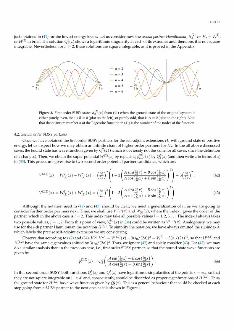
1 (z). Thesefunctions have not been considered as solutions of our problem, since they show singularities within the open interval(−a, a) and are not square integrable, as shown in the Appendix. In Figure 3, we represent some of the wave equations

11 of 17

just obtained in (41) for the lowest energy levels. Let us consider now the second partner Hamiltonian, H(2)α := Hα + V(2)

α ,or H(2) in brief. The solution Q1

1(z) shows a logarithmic singularity at each of its extremes and, therefore, it is not squareintegrable. Nevertheless, for n ≥ 2, these solutions are square integrable, as it is proved in the Appendix.

- s02 a

s02 a

n 2

n 3

n 4

n 5

n 6

- s02 a

s02 a

Figure 3. First order SUSY states φ(2)n (x) from (41) when the ground state of the original system is

either purely even, that is B = 0 (plot on the left), or purely odd, that is A = 0 (plot on the right). Notethat the quantum number n of the Legendre function in (41) is the number of the nodes of the function.

4.2. Second order SUSY partners

Once we have obtained the first order SUSY partners for the self-adjoint extensions Hα with ground state of positiveenergy, let us inspect how we may obtain an infinite chain of higher order partners for Hα. In the all above discussedcases, the bound state has wave function given by Q2

1(z) (which is obviously not the same for all cases, since the definition

of z changes). Then, we obtain the super-potential W(2)(x) by replacing φ(0)n=1(x) by Q2

1(z) (and then write z in terms of x)in (33). This procedure gives rise to two second order potential partner candidates, which are:

V(2,1)(x) = W2(2)(x)−W ′(2)(x) =

( s0

2a

)21 + 2

(A sin

( s02a x)− B cos

( s02a x)

A cos( s0

2a x)+ B sin

( s02a x))2

− 3( s0

2a

)2, (42)

V(2,2)(x) = W2(2)(x) + W ′(2)(x) =

( s0

2a

)21 + 3

(A sin

( s02a x)− B cos

( s02a x)

A cos( s0

2a x)+ B sin

( s02a x))2

. (43)

Although the notation used in (42) and (43) should be clear, we need a generalization of it, as we are going toconsider further order partners next. Thus, we shall use V(i,j)(x) and W(i)(x), where the index i gives the order of thepartner, which in the above case is i = 2. This index may take all possible values i = 1, 2, 3, . . . The index j always takestwo possible values, j = 1, 2. From this point of view, V(i)

α (x) in (34) could be written as V(1,i)(x). Analogously, we mayuse for the i-th partner Hamiltonian the notation H(i,j). To simplify the notation, we have always omitted the subindex α,which labels the precise self-adjoint extension we are considering.

Observe that according to (42) and (34), V(2,1)(x) = V(1,2)(x)− 3(s0/(2a))2 = V(2)α − 3(s0/(2a))2, so that H(2,1) and

H(1,2) have the same eigenvalues shifted by 3(s0/(2a))2. Thus, we ignore (42) and solely consider (43). For (43), we maydo a similar analysis than in the previous case, i.e., first order SUSY partner, so that the bound state wave functions aregiven by

φ(2,2)n (x) = Qn

2

(iA sin

( s02a x)− B cos

( s02a x)

A cos( s0

2a x)+ B sin

( s02a x)) . (44)

In this second order SUSY, both functions Q12(z) and Q2

2(z) have logarithmic singularities at the points x = ±a, so thatthey are not square integrable on [−a, a] and, consequently, should be discarded as proper eigenfunctions of H(2,2). Thus,the ground state for H(2,2) has a wave function given by Q3

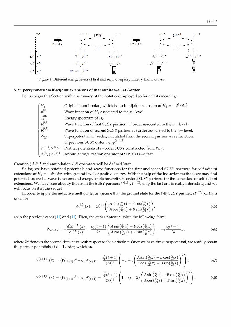
2(z). This is a general behaviour that could be checked at eachstep going from a SUSY partner to the next one, as it is shown in Figure 4.

12 of 17

Figure 4. Different energy levels of first and second supersymmetry Hamiltonians.

5. Supersymmetric self-adjoint extensions of the infinite well at `-order

Let us begin this Section with a summary of the notation employed so far and its meaning:

Hα Original hamiltonian, which is a self-adjoint extension of H0 = −d2/dx2.

φ(0)n Wave function of Hα associated to the n−level.

E(0)n Energy spectrum of Hα.

φ(i,1)n Wave function of first SUSY partner at i order associated to the n− level.

φ(i,2)n Wave function of second SUSY partner at i order associated to the n− level.

W(i) Superpotential at i order, calculated from the second partner wave function.

of previous SUSY order, i.e. φ(i−1,2)i .

V(i,1), V(i,2) Partner potentials of i−order SUSY constructed from W(i).A(i), (A(i))† Annihilation/Creation operator of SUSY at i−order.

Creation (A(i))† and annihilation A(i) operators will be defined later.So far, we have obtained potentials and wave functions for the first and second SUSY partners for self-adjoint

extensions of H0 = −d2/dx2 with ground level of positive energy. With the help of the induction method, we may findpotentials as well as wave functions and energy levels for arbitrary order ` SUSY partners for the same class of self-adjointextensions. We have seen already that from the SUSY partners V(i,1), V(i,2), only the last one is really interesting and wewill focus on it in the sequel.

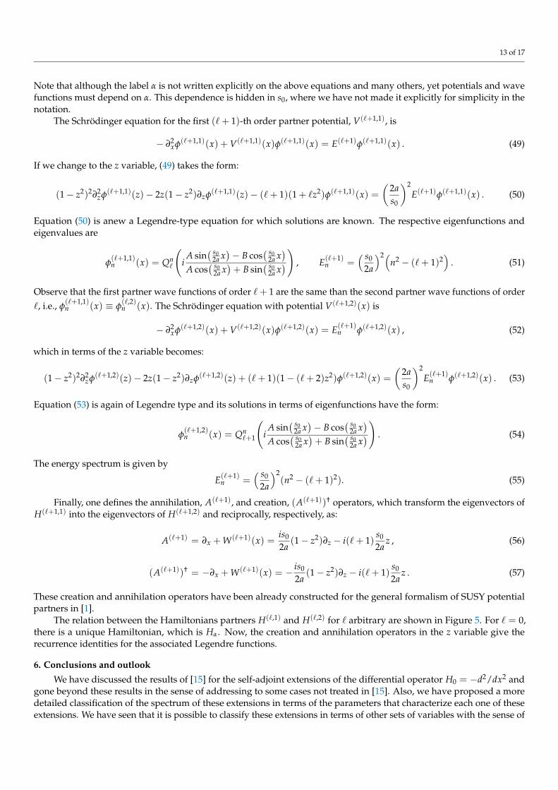
In order to apply the inductive method, let us assume that the ground state for the `-th SUSY partner, H(`,2), of Hα isgiven by

φ(`,2)`+1 (x) = Q`+1

`

(iA sin

( s02a x)− B cos

( s02a x)

A cos( s0

2a x)+ B sin

( s02a x)), (45)

as in the previous cases (41) and (44). Then, the super-potential takes the following form:

W(`+1) = −∂2

xφ(`,2)(x)φ(`,2)(x)

=s0(`+ 1)

2a

(A sin

( s02a x)− B cos

( s02a x)

A cos( s0

2a x)+ B sin

( s02a x)) = −i

s0(`+ 1)2a

z , (46)

where ∂2x denotes the second derivative with respect to the variable x. Once we have the superpotential, we readily obtain

the partner potentials at `+ 1 order, which are

V(`+1,1)(x) = (W(`+1))2 − ∂xW(`+1) =

s20(`+ 1)(2a)2

−1 + `

(A sin

( s02a x)− B cos

( s02a x)

A cos( s0

2a x)+ B sin

( s02a x))2

, (47)

V(`+1,2)(x) = (W(`+1))2 + ∂xW(`+1) =

s20(`+ 1)(2a)2

1 + (`+ 2)

(A sin

( s02a x)− B cos

( s02a x)

A cos( s0

2a x)+ B sin

( s02a x))2

. (48)

13 of 17

Note that although the label α is not written explicitly on the above equations and many others, yet potentials and wavefunctions must depend on α. This dependence is hidden in s0, where we have not made it explicitly for simplicity in thenotation.

The Schrödinger equation for the first (`+ 1)-th order partner potential, V(`+1,1), is

− ∂2xφ(`+1,1)(x) + V(`+1,1)(x)φ(`+1,1)(x) = E(`+1)φ(`+1,1)(x) . (49)

If we change to the z variable, (49) takes the form:

(1− z2)2∂2zφ(`+1,1)(z)− 2z(1− z2)∂zφ(`+1,1)(z)− (`+ 1)(1 + `z2)φ(`+1,1)(x) =

(2as0

)2E(`+1)φ(`+1,1)(x) . (50)

Equation (50) is anew a Legendre-type equation for which solutions are known. The respective eigenfunctions andeigenvalues are

φ(`+1,1)n (x) = Qn

`

(iA sin

( s02a x)− B cos

( s02a x)

A cos( s0

2a x)+ B sin

( s02a x)) , E(`+1)

n =( s0

2a

)2(n2 − (`+ 1)2

). (51)

Observe that the first partner wave functions of order `+ 1 are the same than the second partner wave functions of order`, i.e., φ

(`+1,1)n (x) ≡ φ

(`,2)n (x). The Schrödinger equation with potential V(`+1,2)(x) is

− ∂2xφ(`+1,2)(x) + V(`+1,2)(x)φ(`+1,2)(x) = E(`+1)

n φ(`+1,2)(x) , (52)

which in terms of the z variable becomes:

(1− z2)2∂2zφ(`+1,2)(z)− 2z(1− z2)∂zφ(`+1,2)(z) + (`+ 1)(1− (`+ 2)z2)φ(`+1,2)(x) =

(2as0

)2E(`+1)

n φ(`+1,2)(x) . (53)

Equation (53) is again of Legendre type and its solutions in terms of eigenfunctions have the form:

φ(`+1,2)n (x) = Qn

`+1

(iA sin

( s02a x)− B cos

( s02a x)

A cos( s0

2a x)+ B sin

( s02a x)) . (54)

The energy spectrum is given by

E(`+1)n =

( s0

2a

)2(n2 − (`+ 1)2). (55)

Finally, one defines the annihilation, A(`+1), and creation, (A(`+1))† operators, which transform the eigenvectors ofH(`+1,1) into the eigenvectors of H(`+1,2) and reciprocally, respectively, as:

A(`+1) = ∂x + W(`+1)(x) =is0

2a(1− z2)∂z − i(`+ 1)

s0

2az , (56)

(A(`+1))† = −∂x + W(`+1)(x) = − is0

2a(1− z2)∂z − i(`+ 1)

s0

2az . (57)

These creation and annihilation operators have been already constructed for the general formalism of SUSY potentialpartners in [1].

The relation between the Hamiltonians partners H(`,1) and H(`,2) for ` arbitrary are shown in Figure 5. For ` = 0,there is a unique Hamiltonian, which is Hα. Now, the creation and annihilation operators in the z variable give therecurrence identities for the associated Legendre functions.

6. Conclusions and outlook

We have discussed the results of [15] for the self-adjoint extensions of the differential operator H0 = −d2/dx2 andgone beyond these results in the sense of addressing to some cases not treated in [15]. Also, we have proposed a moredetailed classification of the spectrum of these extensions in terms of the parameters that characterize each one of theseextensions. We have seen that it is possible to classify these extensions in terms of other sets of variables with the sense of

14 of 17

Figure 5. Energy scheme of different SUSY transformations until `-order.

angles, which permits to go beyond [15]. These self-adjoint extensions may have at most two negative eigenvalues, aground state of zero energy and ground states with strictly positive energy.

In addition, in this paper, we have obtained analytically the form of the SUSY partners for the self-adjoint extensionsof H0 (that we denote as Hα, where α includes the four real parameters that gives each of these extensions) with groundstate with positive energy. We have obtained all Hamiltonian partners of each of the Hα with positive spectrum to allorders, their energy levels and their eigenfunctions. At each step, we find two distinct Hamiltonian partners of `-th order.Creation and annihilation operators related the eigenfunctions for these two partners were also evaluated.

Although we have obtained the eigenfunctions for the whole sequence of SUSY partners of each of the Hα, theseeigenfunctions depend explicitly depends on the square root of the ground state energy of Hα, which in most cases can beobtained by solving a transcendental equation. However, this transcendental equation looks rather intractable in a fewcases. This situation pose some difficulties in order to obtain the eigenvalues for some of the Hα, although the explicitform of their eigenfunctions and of the eigenfunctions of their SUSY partners can always be given, as functions of thesquare root of the ground state energy of Hα.

We have not obtained the SUSY partners for those extensions, Hα, with ground state with zero or negative energy.Here, we may also obtain a sequence of SUSY partners form each of the Hα in this class. Unlike to the partners forextensions Hα with ground state with strictly positive energies, these partners may have a finite number of eigenvaluesor even none and the potential partners may show singularities. A classification of the partners for these exceptionalextensions is left for a forthcoming paper.

Author Contributions: All authors listed have made a substantial, direct, and intellectual contribution to the work. All authors haveread and agreed to the published version of the manuscript.

Funding: This research was funded by Junta de Castilla y León and FEDER projects VA137G18 and BU229P18.

Conflicts of Interest: The authors declare no conflict of interest. The funders had no role in the design of the study; in the collection,analyses, or interpretation of data; in the writing of the manuscript, or in the decision to publish the resultss.

References1. Fernández, D.J. Supersymmetric quantum mechanics. AIP Conference Proceedings, 2010, 1287, 3–36.2. Infeld, L; Hull, T.E.; The factorization method. Rev. Mod. Phys. 1951, 23, 21–68.3. Lahiri, A; Roy, P.K., Bagchi, B. Supersymmetry in quantum mechanics. Int. J. Mod. Phys. A 1990, em 5 1383-1456.4. Roy, B; Roy, P; Roychoudhury, R. On the solution of quantum eigenvalue problems. A supersymmetric point of view. Fort. Phys.

1991, 39, 211-258.5. Bagchi, B. Superymmetry in Quantum and Classical Mechanics. Chapman and Hall: Boca Raton, USA, 2001.6. Cooper, F.; Khare, A.; Sukhatme, U. Supersymmetry and Quantum Mechanics. Phys.Rep 1995, 251, 267–385.7. Díaz, J.I.; Negro, J; Nieto, L.M.; Rosas-Ortiz, O. The supersymmetric modified Pöschl-Teller and delta-well potential. J. Phys A:

Math. Gen. 1999, 32, 8447–8460.8. Mielnik, B.; Nieto, L.M.; Rosas-Ortiz, O. The finite difference algorithm for higher order supersymmetry. Phys. Lett. A 2000, 269,

70–78.9. Fernández C, D.J.; Negro, J; Nieto, L.M. Regularized Scarf potentials: energy band structure and supersymmetry. J. Phys A: Math.

Gen. 2004, 37, 6987–7001.10. Ioffe, M.V.; Negro, J; Nieto, L.M.; Nishiniandze, D. New two-dimensional integrable quantum models from SUSY intertwining. J.

Phys A: Math. Gen. 2006, 39, 9297–9308.11. Correa, F; Nieto, L.M.; Plyushchay, M.S. Hidden nonlinear supersymmetry of finite-gap Lamé equation. Phys. Lett. B 2007, 644,

94–98.

15 of 17

12. Ganguly, A.; Nieto, L.M. Shape-invariant quantum Hamiltonian with position-dependent effective mass through second-ordersupersymmetry. J. Phys A: Math. Gen. 2007, 49, 7265–7281.

13. Correa, V.; Jakubsk, V.; Nieto, L.M.; Plyushchay, M.S. Self-isospectrality, special supersymmetry, and their effect on the bandstructure. Phys. Rev. Lett. 2008, 101, 030403.

14. Fernández C, D.J.; Gadella, M.; Nieto, L.M.; Supersymmetry Transformations for Delta Potentials. SIGMA 2011, 7, 029.15. Bonneau, G.; Faraut, J.; Valent, G. Self adjoint extensions of operators and the teaching of Quantum Mechanics. Am. J. Phys. 2001,

69, 322-331.16. Albeverio, S.; Fassari, S.; Rinaldi, F. The Hamiltonian of the harmonic oscillator with an attractive δ′-interaction centred at the

origin as approximated by the one with a triple of attractive delta-interactions. J. Phys. A: Math. Theor. 2016, 49, 025302.17. Zolotaryuk, A.V.; Tsironis, G.P.; Zolotaryuk, Y. Point Interactions With Bias Potentials. Frontiers in Physics 2019 7, 87.18. Zolotaryuk, A.V. A phenomenon of splitting resonant-tunneling one-point interactions. Ann. Phys. 2018, 396, 479–494.19. Zolotaryuk, A.V.; Zolotaryuk, Y. A zero-thickness limit of multilayer structures: a resonant-tunnelling δ′-potential. J. Phys. A:

Math. Theor. 2015, 48, 035302 .20. Golovaty, Yu. D.; Hryniv, R.O. On norm resolvent convergence of Schrödinger operators with δ′-like potentials. J. Phys. A: Math.

Theor. 2010, 43, 155204 .21. Erman, F.; Uncu, H. Green’s function formulation of multiple nonlinear Dirac delta-function potential in one dimension. Phys.

Lett. A 2020, 384, 126227.22. Donaire, M.; Muñoz-Castañeda, J.M.; Nieto, L.M.; Tello-Fraile, M. Field Fluctuations and Casimir Energy of 1D-Fermions.

Symmetry 2019, 11, 643. https://doi.org/10.3390/sym1105064323. Gadella, M.; Mateos-Guilarte, J.M.; Muñoz-Castañeda, J.M.; Nieto, L.M. Two-point one-dimensional δ(x)− δ′(x) interactions:

non-abelian addition law and decoupling limit. J. Phys. A: Math. Theor. 2016, 49, 015204.24. Gadella, M.; Mateos-Guilarte, J.M.; Muñoz-Castañeda, J.M.; Nieto, L.M.; Santamaría-Sanz, L. Band spectra of periodic hybrid δ-δ′

structures. Eur. Phys. J. Plus 2020, 135, 786.25. Reed, M.; Simon, B.; Fourier Analysis. Self Adjointness; Academic Press: New York, USA,1975.26. Fassari, S.; Gadella, M.; Glasser, M.L.; Nieto, L. M. Spectroscopy of a one-dimensional V-shaped quantum well with a point

impurity. Ann. Phys. 2018, 389, 48-62.27. Kurasov, P. Distribution theory for discontinuous test functions and differential operators with generalized coefficients. J. Math.

Ann. Appl. 1996, 201, 297-323.28. Charro, M.E.; Glasser, M.L.; Nieto, L.M. Dirac Green function for δ potentials. EPL 2017, 120, 30006.29. Fassari, S.; Gadella, M.; Nieto, L. M.; Rinaldi, F. On the spectrum of the one-dimensional Schrödinger Hamiltonian perturbed by

an attractive Gaussian potential. Acta Politechnica 2017, 57, 385-390.30. Muñoz-Castañeda, J.M.; Nieto, L.M.; Romaniega, C. Hyperspherical δ− δ′ potentials. Ann. Phys. 2019, 400, 246-261.31. Albeverio, S.; Fassari, S.; Gadella, M.; Nieto, L.M.; Rinaldi, F. The Birman-Schwinger Operator for a Parabolic Quantum Well in a

Zero-Thickness Layer in the Presence of a Two-Dimensional Attractive Gaussian Impurity. Front. Phys. 2019, 7, 102.32. Gadella, M.; García-Ferrero, M.A.; González-Martín, S.; Maldonado-Villamizar, F.H. The infinite square well with a point

interaction: A discussion on the different parameterizations. Int. J. Theor. Phys. 2013, 53, 1614-1627.33. Gadella, M.; Glasser, M.L.; Nieto, L.M. The infinite square well with a singular perturbation. Int. J. Theor. Phys., 2011, 50,

2191–2200.34. Naimark, M.A. Linear Differential Operators; Dover: New York, USA, 2014.35. Gadella, M.; Glasser, M.L.; Nieto, L.M. One Dimensional Models with a Singular Potential of the Type −α δ(x) + βδ′(x). Int. J.

Theor. Phys., 2011, 50, 2144-2152.36. Reed, M; Simon, B.; Functional Analysis; Academic Press: New York, USA, 1972.37. Bachman, G; Narici, L; Functional Analysis; Dover: New York, USA, 2012.38. Olver, F.W.J.; Lozier, D.W.; Boisvert, R.F.; Clark, C.W. NIST Handbook of Mathematical Functions, 1st ed.; Cambridge University

Press: Publisher Location, UK, 2010. https://dlmf.nist.gov/14.3,

Appendix A

In this Appendix, we justify the correct choice of the wave functions for the bound states of the supersymmetricpartners of each of the extensions Hα with strictly positive ground state energy. In Appendix A.1, we derive a generalsolution for these wave functions as a linear combination of the associated Legendre functions Pn

` and Qn` with argument

− tan((s0x)/(2a)). In Appendix A.2, we show that the component with Pn` should be discarded, since it does not meet

the requirement of square integrability. On the other hand, the component with Qn` should give the wave function as is

square integrable, as proven in Appendix A.3.

Appendix A.1

Comments in these Appendices are valid for those self-adjoint extensions Hα with ground states with positive energy.For each of these extensions, the ground state energy is E(0)

0 = (s0/(2a))2, where s0 depends on the chosen self-adjointextensions and, therefore, on the values of the parameters. As we have seen, in terms of the auxiliary variable s, the

16 of 17

spectrum is equally spaced in this case, so that all other energy values are E(0)m = (s0/(2a))2m2. For the ground state, the

wave function isφ(0)m=1(x) = A cos

( s0

2ax)+ B sin

( s0

2ax)

. (A1)

The coefficients A and B, as complex numbers, should have the same phase in order to have a real partner potential. Tosee it, let us write A = Ceiϕ1 and B = Deiϕ2 , with C := |A| and D := |B|. Then, (A1) is

φ(0)m=1(x) = Ceiϕ1 cos

( s0

2ax)+ Deiϕ2 sin

( s0

2ax)

. (A2)

Using Definitions (42) and (43) for the potential partners of `-th order, we have for the first `-th partner:

V(`+1,1) =s2

0(`+ 1)(2a)2

−1 + `

(Ceiϕ1 sin

( s02a x)− Deiϕ2 cos

( s02a x)

Ceiϕ1 cos( s0

2a x)+ Deiϕ2 sin

( s02a x))2

, (A3)

for which the imaginary part is given by

Im(

V(`+1,1))= Im

s20(`+ 1)(2a)2

−1 + `

(A sin

( s02a x)− B cos

( s02a x)

A cos( s0

2a x)+ B sin

( s02a x))2

=CD`(`+ 1)s2

0((C− D)(C + D) sin

( s0xa)− 2CD cos(ϕ1 − ϕ2) cos

( s0xa))

a2(2CD cos(ϕ1 − ϕ2) sin

( s0xa)+ (C− D)(C + D) cos

( s0xa)+ C2 + D2

)2 sin(ϕ1 − ϕ2) , (A4)

so that potential (A3) is real if sin(ϕ1 − ϕ2) = 0, or equivalently, if ϕ1 = nπ + ϕ2. Thus, if A and B have the same phaseas complex numbers, we have guaranteed that the potential partner V(`+1,1) is real. The same is valid for V(`+1,2). Thus,(A2) becomes:

φ(0)m=1(x) = Ceiϕ cos

( s0

2ax)+ Deiϕ sin

( s0

2ax)

. (A5)

This ground state is not yet normalized. Its normalization gives∫ a

−adx φ

(0)m=1(x)

(φ(0)m=1(x)

)∗= 1 =⇒ C2 + D2 = 1 =⇒ C = cos δ, D = sin δ . (A6)

Finally, the ground state wave function has the form:

φ(0)m=1(x) = eiϕ cos

( s0

2ax + δ

). (A7)

Let us recall that our goal is to show that the solution of the Schrödinger equation with component Qn` is square integrable

and the solution with Pn` is not. To begin with, let us define a new independent variable using the shift x = y− 2aδ/s0.

The ground state has now the form,

φ(0)m=1 = eiϕ cos

( s0

2ay)

. (A8)

With this notation, the wave function of the second partner of `-th order is

φ(`,2)m = C1Pn

`

(−i tan

( s0y2a

))+ C2Qn

`

(−i tan

( s0y2a

)). (A9)

Next, we shall analyze the square integrability of each of the components in (A9).

17 of 17

Appendix A.2 Trigonometric expansion of Pn`

(−i tan

( s0y2a))

Let us use the change of variable z = −i tan( s0y

2a)

and consider the hypergeometric form of the associated Legendrefunctions with argument z [38]:

Pn` (z) =

1`!

(−1

2

)`(1 + z1− z

)n/2(1− z)`

Γ(2`+ 1) 2F1(−`, n− `;−2`;− 2

z−1)

Γ(`− n + 1)

=1`!

(−1

2

)`(1 + z1− z

)n/2(1− z)`

`

∑j=0

((2`− j)!(−`)j

)j!Γ(−j + `− n + 1)

(2

1− z

)j

=

(− 1

2

)`Γ(2`+ 1)

`!Γ(`− n + 1)e−

is0(n−`)2a y

cos`( s0y

2a) `

∑j=0

(−1)jΓ(`+ 1)(2`− j)!j!Γ(−j + `+ 1)Γ(−j + `− n + 1)

(2e−

is02a y cos

( s0y2a

))j

=`

∑j=0

(−1)j+`2j−`Γ(`+ 1)(2`− j)!j!`!Γ(−j + `+ 1)Γ(−j + `− n + 1)

e−is0y(j−`+n)

2a cosj−`( s0y

2a

). (A10)

Due to the presence of negative powers of the cosine in (A10), the resulting wave function is not square integrable and,therefore, not acceptable as a wave function of a bound state.

Appendix A.3 Trigonometric expansion of Qn` (−i tan

( s0y2a))

Similarly, we can express Qn` (z) in terms of a hypergeometric function [38] as:

Qn` (z) =

1√π

2−`−1(−1)`+n+1(z− 1)−`−1Γ(−`− 1

2

)(z + 1z− 1

)n/2(`+ n)! 2F1

(`+ 1, `+ n + 1; 2(`+ 1);− 2

z− 1

).

Then, let us perform again the change of variables given by z = −i tan( s0y

2a), so as to obtain:

Qn`

(−i tan

( s0y2a

))=

1√π

2−`−1(−1)nΓ(−`− 1

2

)Γ(`+ n + 1)e−i s0

2a y(`+n+1) cos`+1( s0y

2a

)× 2F1

(`+ 1, `+ n + 1; 2(`+ 1); 2e−i s0y

2a cos( s0y

2a

)).

If again, we perform a series expansion around z = 0 we obtain the following power series in terms of positive powers ofcosines:

Qn`

(−i tan

( s0y2a

))=

12(−1)−`+n+1e−i s0

2a nyΓ(n− `)Γ(`+ n + 1)n

∑j=`+1

(−1)jΓ(j) 2jeij s02a y

Γ(j− `)Γ(j + `+ 1)Γ(−j + n + 1)cosj

( s0

2ay)

.

This solution is acceptable as is square integrable.