BASES OF INFINITE-DIMENSIONAL REPRESENTATIONS OF

ORTHOSYMPLECTIC LIE SUPERALGEBRAS

by

DWIGHT ANDERSON WILLIAMS II

Presented to the Faculty of the Graduate School of

The University of Texas at Arlington in Partial Fulfillment

of the Requirements

for the Degree of

DOCTOR OF PHILOSOPHY

THE UNIVERSITY OF TEXAS AT ARLINGTON

May 2020

Copyright c© by Dwight Anderson Williams II 2020

All Rights Reserved

ACKNOWLEDGEMENTS

God is the only mathematician who should say that the proof is trivial. Thank

you God for showing me well-timed hints and a few nearly-complete solutions.

“The beginning of the beginning.” Thank you Dimitar Grantcharov for advising

me, for allowing your great sense of humor, kindness, brilliance, respect, and mathe-

matical excellence to easily surpass your great height–it is an honor to look up to

you and to look forward towards continued collaboration.

Work done by committee Thank you to my committe members (alphabetically

listed by surname): Edray Goins, David Jorgensen, Christopher Kribs, Barbara

Shipman, and Michaela Vancliff.

April 30, 2020

iii

ABSTRACT

BASES OF INFINITE-DIMENSIONAL REPRESENTATIONS OF

ORTHOSYMPLECTIC LIE SUPERALGEBRAS

Dwight Anderson Williams II, Ph.D.

The University of Texas at Arlington, 2020

Supervising Professor: Dimitar Grantcharov

We provide explicit bases of representations of the Lie superalgebra osp(1|2n)

obtained by taking tensor products of infinite-dimensional representation and the

standard representation. This infinite-dimensional representation is the space of

polynomials C[x1, . . . , xn]. Also, we provide a new differential operator realization of

osp(1|2n) in terms of differential operators of n commuting variables x1, . . . , xn and

2n anti-commuting variables ξ1, . . . , ξ2n.

iv

TABLE OF CONTENTS

ACKNOWLEDGEMENTS . . . . . . . . . . . . . . . . . . . . . . . . . . . . iii

ABSTRACT . . . . . . . . . . . . . . . . . . . . . . . . . . . . . . . . . . . . iv

Chapter Page

1. Introduction . . . . . . . . . . . . . . . . . . . . . . . . . . . . . . . . . . . 1

1.1 History of Supermathematics . . . . . . . . . . . . . . . . . . . . . . 1

1.2 Superalgebras . . . . . . . . . . . . . . . . . . . . . . . . . . . . . . . 2

1.3 Orthosymplectic Lie Superalgebras . . . . . . . . . . . . . . . . . . . 3

1.4 Representation Theory of osp(1|2n) . . . . . . . . . . . . . . . . . . . 3

1.5 Notation & Conventions . . . . . . . . . . . . . . . . . . . . . . . . . 4

2. Groups, Rings, Vector Spaces . . . . . . . . . . . . . . . . . . . . . . . . . 6

2.1 Basic Definitions . . . . . . . . . . . . . . . . . . . . . . . . . . . . . 6

2.2 Classical Examples . . . . . . . . . . . . . . . . . . . . . . . . . . . . 10

2.2.1 Forms on a Vector Space . . . . . . . . . . . . . . . . . . . . . 10

2.2.2 Classical Groups . . . . . . . . . . . . . . . . . . . . . . . . . 16

3. Algebras . . . . . . . . . . . . . . . . . . . . . . . . . . . . . . . . . . . . . 20

3.1 Algebra of Endomorphisms and Free Algebras . . . . . . . . . . . . . 21

3.2 Tensor Algebras and Quotients . . . . . . . . . . . . . . . . . . . . . 23

3.2.1 Weyl and Symmetric Algebras . . . . . . . . . . . . . . . . . . 25

3.2.2 Clifford and Exterior Algebras . . . . . . . . . . . . . . . . . . 26

3.3 Non-associative Algebras & Universal Enveloping Algebras . . . . . . 27

3.3.1 Lie algebras . . . . . . . . . . . . . . . . . . . . . . . . . . . . 27

3.3.2 Universal Enveloping Algebras & Representation Theory . . . 31

v

4. Superalgebras . . . . . . . . . . . . . . . . . . . . . . . . . . . . . . . . . . 37

4.1 Super Linear Algebra . . . . . . . . . . . . . . . . . . . . . . . . . . . 38

4.2 Lie Superalgebras . . . . . . . . . . . . . . . . . . . . . . . . . . . . . 40

4.2.1 The general linear Lie superalgebra . . . . . . . . . . . . . . . 42

4.2.2 Modules of Lie superalgebras . . . . . . . . . . . . . . . . . . 43

4.3 Associative superalgebras . . . . . . . . . . . . . . . . . . . . . . . . . 44

4.3.1 Universal enveloping algebras of Lie superalgebras . . . . . . . 44

4.4 Weyl superalgebras . . . . . . . . . . . . . . . . . . . . . . . . . . . . 46

5. Orthosymplectic Lie Superalgebras . . . . . . . . . . . . . . . . . . . . . . 48

5.1 The Lie Superalgebra osp(1|2n) . . . . . . . . . . . . . . . . . . . . . 48

5.1.1 Root System of osp(1|2n) . . . . . . . . . . . . . . . . . . . . 50

5.1.2 Root Vectors of osp(1|2n) . . . . . . . . . . . . . . . . . . . . 51

5.1.3 Root Vector Relations for osp(1|2n) . . . . . . . . . . . . . . . 52

5.1.4 C1|2n as an osp(1|2n)-module . . . . . . . . . . . . . . . . . . 54

5.2 Super Module Theory . . . . . . . . . . . . . . . . . . . . . . . . . . 55

5.2.1 Highest Weight Modules and Primitive Vectors . . . . . . . . 55

5.2.2 Tensor products of weight modules . . . . . . . . . . . . . . . 55

5.2.3 Weyl superalgebra homomorphism . . . . . . . . . . . . . . . 56

5.2.4 Primitive Vectors of Tensor Products of osp(1|2n)-modules . . 56

6. Bases of a Direct Sum and Formulas . . . . . . . . . . . . . . . . . . . . . 58

6.1 Notation . . . . . . . . . . . . . . . . . . . . . . . . . . . . . . . . . . 58

6.2 First Main Result . . . . . . . . . . . . . . . . . . . . . . . . . . . . . 59

6.2.1 The Super Subspaces V 0 and V + . . . . . . . . . . . . . . . . 59

6.2.2 Defining New Operators on V . . . . . . . . . . . . . . . . . . 60

6.2.3 Obtaining Submodules of V through New Operators . . . . . 60

6.2.4 Main Theorem I . . . . . . . . . . . . . . . . . . . . . . . . . . 64

vi

6.3 Mixed Images . . . . . . . . . . . . . . . . . . . . . . . . . . . . . . . 66

7. New Differential Operator Realizations . . . . . . . . . . . . . . . . . . . . 69

7.1 New “Psi” Operators . . . . . . . . . . . . . . . . . . . . . . . . . . . 69

7.2 Second Main Result . . . . . . . . . . . . . . . . . . . . . . . . . . . . 70

7.2.1 Relations on the New “Psi” . . . . . . . . . . . . . . . . . . . 70

7.2.2 Main Theorem II . . . . . . . . . . . . . . . . . . . . . . . . . 77

7.2.3 New Idea . . . . . . . . . . . . . . . . . . . . . . . . . . . . . 78

REFERENCES . . . . . . . . . . . . . . . . . . . . . . . . . . . . . . . . . . . 79

BIOGRAPHICAL STATEMENT . . . . . . . . . . . . . . . . . . . . . . . . . 83

vii

CHAPTER 1

Introduction

The current work is an investigation concerning the infinite-dimensional super

representation theory of the family of complex orthosymplectic Lie superalgebras

osp(1|2n,C). The results relate broadly to the algebraic corners of supermathematics,

which has both mathematical and physical foundations.

1.1 History of Supermathematics

The popularization of supermathematics is largely due to the writings of Felix

Berezin. Posthumously, Berezin’s manuscripts were translated into English from

Russian and his colleagues edited [3], in which there is an extensive account of

supermathematics with the mathematician in mind. The mathematical emphasis

is important as supermathematics is a term credited to physicists and much of the

motivation for the theory stems from physical problems. Algebraically, the formulation

of supermathematics involves heavily the study of objects in the symmetric monoidal

category of Z2-graded vector spaces adhering to a twisted braiding. That is, the

category with super vector spaces as objects and parity-preserving linear maps

as morphisms has a braiding on the tensor product related to the Koszul sign

rule such that exchanging odd elements results in negation. Super vector spaces

underlie (supercommutative and associative) superalgebras. As in the classical

case, an important example of superalgebras arises from considering functions on

a space, one now having both commutative and anti-commutative coordinates or

values in a Grassmann algebra as described in [2]. A sheaf-theoretic viewpoint uses

1

these superfunctions to define supermanifolds and Lie supergroups. Appropriately,

associated to a Lie supergroup is a Lie superalgebra, however the present discussion

will align with a far more algebraic approach to Lie superalgebras and superalgebras.

1.2 Superalgebras

In 1941, Whitehead defined a product on the graded homotopy groups of

a pointed topological space, the first non-trivial example of a Lie superalgebra.

Whitehead’s work in algebraic topology [41] was known to mathematicians who defined

new graded geo-algebraic structures, such as Z2-graded algebras, or superalgebras to

physicists, and their modules. A Lie superalgebra g = g0 ⊕ g1 would come to be a

Z2-graded vector space, even (espectively, odd) elements found in g0 (respectively, g1),

with a parity-respecting bilinear multiplication [·, ·], the Lie superbracket, that satisfies

[x, [x, x]] = 0 for all x ∈ g1 and induces a symmetric intertwining map g1⊗g1 → g0 of

(g0, [·, ·]∣∣g0

)-modules [5]. Researchers of the 1960s and 1970s furthered the systematic

study of Lie superalgebras with a view for supermanifolds and the need for physicists

to extend the classical symmetry formulation behind Wigner’s Nobel Prize to one

incorporating bosonic (“even”) and fermionic (“odd”) particles simultaneously—the

famed supersymmetry (SUSY) [see 12, 44]. As mentioned above, supermathematics

has become synonymous with the study of Z2-graded structures and spaces with

Grassmann-valued coordinates. Now the algebraic development of supermathematics

in terms of Lie superalgebras has become its own source of motivation—even providing

a dictionary [15]—beginning with the classification of simple finite-dimensional Lie

superalgebras over algebraically closed fields of characteristic zero in [23].

2

1.3 Orthosymplectic Lie Superalgebras

Specifically, the Lie superalgebra osp(1|2n,R) is of great importance to su-

perconformal theories; see chapters 6 and 7 of [11] for an early survey of physical

applications. The natural purusit to describe simple objects in a module category of

osp(1|2n,C), and of other classical Lie superalgebras defined in [24], was considered

by Dimitrov, Mathieu, Penkov in [9]. Gorelik and Grantcharov completed the clas-

sification began in [9] by publishing [14] then [18], the former with Ferguson, who

classified the simple bounded highest-weight modules of osp(1|2n,C) in his disserta-

tion [13]. Primitive vectors in certain tensor product representations of osp(1|2n,C)

were essential to the completion of [13]. Coulembier also paid close attention to

primitive vectors in [7] to determine whether tensor products of certain irreducible

highest-weight osp(2m+ 1|2n,R)-representations were completely reducible; a series

of papers by Coulembier and co-authors [6, 7, 8] motivated inspecting the reducibility

of certain osp(1|2n,R)-modules to establishing a Clifford analysis on supermanifolds.

The case of m = 0 over C is considered herein.

1.4 Representation Theory of osp(1|2n)

This dissertation focuses on the infinite-dimensional (super) representation

theory of the complex orthosymplectic Lie superalgebra B(0|n) [23].1 In detail, the

present exposition recalls necessary definitions and concepts of multilinear algebra in

Chapter 2, of algebras in Chapters 3, of superalgebras in Chapter 4, and of orthosym-

plectic Lie superalgebras in Chapter 5. Now a classical pursuit in representation

theory is to consider tensor products of infinite-dimensional representations with finite-

dimensional representations as in [4, 25, 43]. Chapter 6 analyzes the tensor product

1The series of Lie superalgebras B(m|n) over a field K of characteristic zero is the series oforthosymplectic algebras osp(2m + 1|2n,K).

3

C[x1, . . . , xn]⊗C1|2n of an infinite-dimensional osp(1|2n)-representation C[x1, . . . , xn]

with the standard osp(1|2n)-representation C1|2n. Primitive vectors play a key role in

the first new result of decomposing C[x1, . . . , xn]⊗C1|2n as an osp(1|2n)-representation

with explicit descriptions of the osp(1|2n)-subrepresentations, including bases. Lastly,

Chapter 7 provides a map of associative superalgebras between the universal en-

veloping Lie superalgebra U(osp(1|2n)) and (super) differential operators inside the

endomorphism superalgebra of C[x1, . . . , xn]⊗ C[ξ1, . . . , ξ2n], where the xi commute

and the ξj anti-commute.

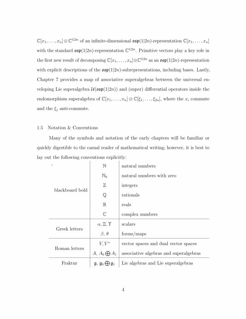
1.5 Notation & Conventions

Many of the symbols and notation of the early chapters will be familiar or

quickly digestible to the casual reader of mathematical writing; however, it is best to

lay out the following conventions explicitly:

‘

blackboard bold

N natural numbers

N0 natural numbers with zero

Z integers

Q rationals

R reals

C complex numbers

Greek lettersα,Ξ,Υ scalars

β, θ forms/maps

Roman lettersV, V ∗ vector spaces and dual vector spaces

A, A0

⊕A1 associative algebras and superalgebras

Fraktur g, g0

⊕g1 Lie algebras and Lie superalgebras

4

A familiarity with the standard topics of a first-year (linear) algebra course is

assumed from the interested reader. Specifically, the reader should be comfortable

with the content found in [1, 38]. A two-semester sequence of graduate algebra is

also recommended.

5

CHAPTER 2

Groups, Rings, Vector Spaces

This chapter serves to recall some definitions found in [22] and other fundamental

treatments of modern algebra. The reader familiar with groups, rings, and vectors

spaces may refer to this chapter for notation and verification of definitions at play.

The end of the chapter provides some standard references to definitions and examples

found in any text on multilinear algebra. Some standard proofs are provided.

2.1 Basic Definitions

Definition 2.1.1. A monoid M is a set of composable transformations of a space.

Axiomatically, a monoid 〈M, , e〉 is a nonempty set M with an associative binary op-

eration called multiplication and a distinguished element e serving as a multiplicative

identity. We often write ab for a b and 1 for e.

Definition 2.1.2. The opposite monoid Mop = 〈M, ∗, e〉 with a ∗ b = ba, for all

a, b ∈ M . The identity 1M : 〈M, , e〉 → 〈M, ∗, e〉 is only a map of monoids if is

commutative.

Example 2.1.3.

6

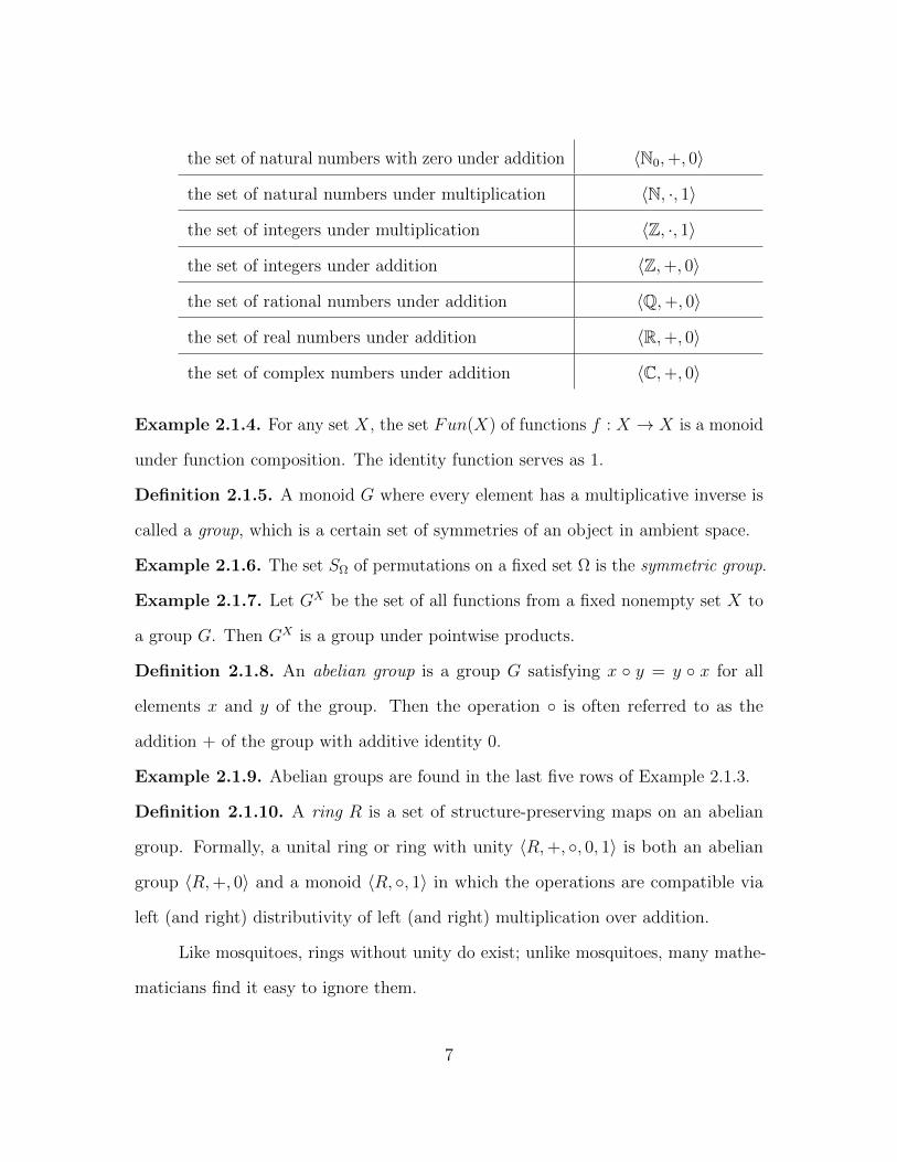
the set of natural numbers with zero under addition 〈N0,+, 0〉

the set of natural numbers under multiplication 〈N, ·, 1〉

the set of integers under multiplication 〈Z, ·, 1〉

the set of integers under addition 〈Z,+, 0〉

the set of rational numbers under addition 〈Q,+, 0〉

the set of real numbers under addition 〈R,+, 0〉

the set of complex numbers under addition 〈C,+, 0〉

Example 2.1.4. For any set X, the set Fun(X) of functions f : X → X is a monoid

under function composition. The identity function serves as 1.

Definition 2.1.5. A monoid G where every element has a multiplicative inverse is

called a group, which is a certain set of symmetries of an object in ambient space.

Example 2.1.6. The set SΩ of permutations on a fixed set Ω is the symmetric group.

Example 2.1.7. Let GX be the set of all functions from a fixed nonempty set X to

a group G. Then GX is a group under pointwise products.

Definition 2.1.8. An abelian group is a group G satisfying x y = y x for all

elements x and y of the group. Then the operation is often referred to as the

addition + of the group with additive identity 0.

Example 2.1.9. Abelian groups are found in the last five rows of Example 2.1.3.

Definition 2.1.10. A ring R is a set of structure-preserving maps on an abelian

group. Formally, a unital ring or ring with unity 〈R,+, , 0, 1〉 is both an abelian

group 〈R,+, 0〉 and a monoid 〈R, , 1〉 in which the operations are compatible via

left (and right) distributivity of left (and right) multiplication over addition.

Like mosquitoes, rings without unity do exist; unlike mosquitoes, many mathe-

maticians find it easy to ignore them.

7

Example 2.1.11. With the usual addition and multiplication, Z, Q, R, C are

commutative rings, which means the multiplication is commutative.

Example 2.1.12. With the same operations as Example 2.1.11, the set of even

integers 2Z forms a commutative ring without unity, while the set of odd integers

2Z+1 fails to satisfy closure of addition. Oddly enough, 〈2Z+1, ·, 1〉 is a commutative

monoid under the usual multiplication of integers.

Remark 2.1.13. We will require a map of unital rings to map unity to unity.

Example 2.1.14. Given a group G and a ring R, we denote the group ring of G over R

by R[G]. We may view R[G] as the set of functions f : G→ R | f has finite support.

The group ring R[G] is commutative if and only if R is commutative and G is abelian.

In particular, for all f : G→ R and g : G→ R in the group ring R[G], we define the

product fg by

fg(z) =∑xy=zx,y∈G

f(x)g(y) =∑x∈G

f(x)g(x−1z).

Example 2.1.15. Let M be an abelian group with more than one element. Let

Fun(M) = MM . As function composition distributes over function addition, Exam-

ple 2.1.4 and Example 2.1.7 define Fun(M) as a noncommutative unital ring. The

ring End(M) of (group) endomorphisms is a subring of Fun(M).

Example 2.1.16. The ring Mat(n,R) consists of n× n matrices with entries from a

ring R under matrix addition and matrix multiplication. Unless n = 1, Mat(n,R) is

a noncommutative ring.

Definition 2.1.17. Division rings are rings where all nonzero elements have a

multiplicative inverse.

Example 2.1.18. A field, such as Q, R, or C, is a commutative division ring.

Definition 2.1.19. An abelian group M upon which each element r of a ring R

acts as a structure-preserving map φr in a compatible manner is called a left module

8

over R or left R-module for short. Compatibility means φrs(m) = φr(φs(m)), written

(rs) ·m = r · (s ·m), ∀m ∈M . Even simpler, we write rm for r ·m.

Definition 2.1.20. A right R-module M is exactly a left Rop-module. The (right)

action m ·∗ r of R on M is defined through the (left) action r ·m of Rop on M .

Intuitively, we gain some data about a choice object by what it does to something

else, usually a vector space. We represent our object of note as transformations of a

familiar space—a representation space—and representation theory is the systematic

investigation into these representations. Modules are the beginning of our interest in

representation theory.

Definition 2.1.21. Modules over a division ring D are called D-vector spaces with

D as the ground ring. Modules over commutative rings R are both left and right

R-modules as R ∼= Rop via the identity map.

Example 2.1.22. The real numbers R and complex numbers C are naturally R-

vector spaces, while the multiplication of C does not define a C-vector space structure

on the reals. More generally, every division ring D is a Z(D)-vector space over its

center Z(D) := z ∈ D | za = az, ∀a ∈ D.

Example 2.1.23. The group EndD(V ) consists of D-linear maps on a D-vector

space V . The dual space V ∗ of V is the set T : V → D | T is a D-linear map.

Both EndD(V ) and V ∗ are D-subspaces inside D-vector spaces Fun(V ) and DV ,

respectively.

We will deal primarily with vector spaces over the complex numbers C. Moreover,

the ground field is assumed to be C, unless otherwise stated, and we will suppress

the ground field from notation when context affords us brevity.

All the usual notions of substructures and quotient structures are standard.

9

2.2 Classical Examples

A broad introduction to Lie algebras involves the areas of differential geometry,

Lie groups, differential equations, functional analysis, and many more subfields of

mathematics along with particle physics. In contrast, this work serves as a narrower

road and quicker path from linear algebra to the main results of my dissertation. Still,

this section may lend both background and motivation into the study of complex

orthosymplectic Lie superalgebras, briefly, sets of linear transformations on Cm+2n

compatible with a geometry expressed algebraically through certain maps from Cm+2n

to C.

In a real and concrete case, we consider R2 with the dot product, v · w =

|v||w| cos θ, as two-dimensional Euclidean space and an example of an inner product

space. Then the geometry of R2 (or of the underlying affine space) is revealed through

distance and angular measurement defined through the dot product. Intuitively, we

see that rotations around a fixed point preserve the dot product while adhering to

the linear structure on the space, and we have the luxury of fixing a basis in order to

represent these transformations as 2×2 matrices. These rotations form a group called

the special orthogonal group of R2. Moreover, this type of set-up finds generalizations

in many other vector spaces. One can explore groups of linear maps that respect both

the vector space structure and the geometry controlled by a form, as defined below.

2.2.1 Forms on a Vector Space

Many algebraic objects described herein are related to maps on vector spaces.

Definition 2.2.1. A multilinear n-form on a vector space V is a map

f : V × V × · · · × V︸ ︷︷ ︸n times

−→ C

10

such that f is linear in each entry. That is, for each i,

f(v1, v2, . . . , xi + yi, vi+1, . . . , vn) = f(v1, v2, . . . , xi, vi+1, vi+1, . . . , vn)

+ f(v1, v2, . . . , yi, vi+1, vi+1, . . . , vn)

and

f(v1, v2, . . . , αxi, vi+1, . . . , vn) = αf(v1, v2, . . . , xi, vi+1, . . . , vn),

with all arguments taken from V and α a complex number. More generally, we can

defined mixed forms on a finite collection of vector spaces of varying dimensions or on

vector spaces of the same dimension. The definition above also describes a multilinear

map where any arbitrary vector space may take the place of the ground field as the

codomain.

For n = 1, 2, 3, we have linear functionals, bilinear forms, and trilinear forms,

respectively. Forms are assumed to be n-linear. For a vector space V with a bilinear

form β, it should be clear that β(0, x) = 0 = β(x, 0), for all x in V .

Recall, Cn is isomorphic to any complex vector space V of dimension n, and the

existence of a linear space isomorphism gives a notion of equivalency amongst spaces.

Now let us use the term bilinear space to describe a vector space with a bilinear form

(V, βV ) and define a map of bilinear spaces f : (V, βV )→ (W,βW ) to be a linear map

f : V → W such that βW (f(x), f(y)) = βV (x, y) for all x, y in V . If f is bijective, as

well, then we call f an isometry and say the bilinear spaces are equivalent. We may

also say the forms themselves are equivalent.

Now the set Bil(V ) of all bilinear forms on a fixed vector space V also has

the structure of a vector space. Both the study of these spaces of forms and the

classification of equivalent forms on V are well-established directions of research along

with interest in a particular space with a given form. As much as linear algebra

11

is a life blood for all of mathematics, the ubiquitous nature of forms is apparent.

Number theoretic questions motivate the classification of equivalent bilinear forms

defined on a vector space over a finite field. The study of real Hilbert spaces is the

study of complete normed vector spaces in which an inner product, a positive-definite

symmetric bilinear form, induces the norm. The complex case for Hilbert spaces

requires sesquilinearity instead of bilinearity. Definitions and examples of the terms

used in this paragraph can be found in any text on functional analysis such as [35] or

[26]. We provide some of the definitions here.

Definition 2.2.2. A bilinear form β : V ×V → C is called a symmetric bilinear form

if β(x, y) = β(y, x), an alternating bilinear form if β(x, x) = 0, and a skew-symmetric

bilinear form if β(x, y) = −β(y, x), for all x, y ∈ V . Each of these type of forms is

an example of a reflexive bilinear form defined by the condition β(x, y) = 0 implies

β(y, x) = 0.

Theorem 2.2.3. Alternating bilinear forms are equivalent to skew-symmetric bilinear

forms.

Proof. We reemphasize that the ground field is C. An alternating bilinear form β and

vectors x and y give 0 = β(x+ y, x+ y) = β(x, x) + β(x, y) + β(y, x) + β(y, y). Thus,

β(x, y) = −β(y, x). In the other direction, a skew-symmetry β implies 2β(x, x) = 0.

Since the characteristic of C is 0 we have β(x, x) = 0.

The proof shows that in any characteristic an alternating bilinear form is skew-

symmetric, and skew-symmetry implies alternativity over fields with characteristic

different from 2. Then the study of bilinear forms on a fixed space V , in some sense,

breaks down to the study of symmetric and skew-symmetric forms on V as any

12

bilinear form β can be expressed as the sum of a symmetric bilinear form βsym and a

skew-symmetric bilinear form βskew:

βsym(x, y) =β(x, y) + β(y, x)

2,(2.1)

βskew(x, y) =β(x, y)− β(y, x)

2.(2.2)

Definition 2.2.4. A reflexive bilinear form β is called a nondegenerate bilinear form

if its (left) radical, denoted here as Radβ = x ∈ V | β(x, y) = 0, ∀y ∈ V , contains

only the zero vector.

Bilinear forms are assumed to be reflexive from now on, but nondegeneracy is

explicitly stated in each case.

Definition 2.2.5. For a subspace W ⊂ V and β a bilinear form on V , denote by

W⊥ the subspace termed the orthogonal complement of W with respect to β. The

orthogonal complement of W is defined to be the set of all vectors in V orthogonal

(precisely, β-orthogonal) to every vector in W :

W⊥ = v ∈ V | β(v, w) = 0, ∀w ∈ W.

In other words, nondegeneracy amounts to the zero vector being the unique

vector orthogonal to all other vectors, i.e., V ⊥ = 0.

For the rest of this section vector spaces will have finite dimension.

Definition 2.2.6. A symplectic bilinear form is a nondegenerate alternating bilinear

form. A pair (V, β) consisting of a vector space with a symplecitc bilinear form is

called a symplectic vector space or just a symplectic space. If the form is possibly

degenerate, then we may speak of an alternating space.

Definition 2.2.7. A symmetric bilinear form β on V defines a unique binary quadratic

form ω : V → C by ω(x) = β(x, x). We will call a pair (V, β) = (V, ω) an orthogonal

space or quadratic space when β is a (not necessarily nondegenerate) symmetric

bilinear form, equivalently, when ω is a (not necessarily nonsingular) quadratic

13

form associated to β as explained below. The form ω has the following properties,

∀α ∈ C, ∀x, y ∈ V :

ω(αx) = α2ω(x)(2.3)

f(x, y) = ω(x+ y)− ω(x)− ω(y) is a symmmetric bilinear form(2.4)

β(x, y) =1

2f(x, y) is the symmetric bilinear form such thatβ(x, x) = ω(x)(2.5)

Thus, β is nondegenerate if and only if ω is nonsingular. Take the previous statement

as a definition.

Here are some results concerning symplectic spaces and quadratic spaces that

may support the results on orthosymplectic spaces found later.

Theorem 2.2.8. If (V, β) is a symplectic space with dim(V ) = n < ∞, then n is

even.

Lemma 2.2.9. Let V be a finite-dimensional vector space with nondegenerate bilinear

form β. If W ⊂ V is a subspace such that β restricted to W×W is also nondegenerate,

then V = W ⊕W⊥.

Proof of Lemma 2.2.9. First note that the map θ : V → W ∗ given by v 7→

βv = β(v,−)∣∣W

is a linear map. As such, dim(V ) = dim(Im θ) + dim(Ker θ).

Since Ker θ = v ∈ V | β(v, w) = 0, ∀w ∈ W = W⊥, we have the inequality

dim(V ) ≤ dim(W ∗) + dim(W⊥) = dim(W ) + dim(W⊥).

Now it remains to show W ∩W⊥ = 0 as dim(W ⊕W⊥) = dim(V ) would follow:

dim(V ) ≤ dim(W ) + dim(W⊥) = dim(W +W⊥) + dim(W ∩W⊥) and W +W⊥ is a

subspace of V .

Write β∣∣W

for β∣∣W×W . The nondegenracy of β

∣∣W

implies that the only element in W

orthogonal to all elements of W is the zero vector. Consequently, if v ∈ W ∩W⊥,

then v = 0.

14

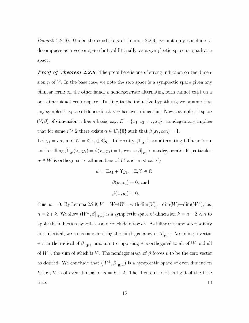
Remark 2.2.10. Under the conditions of Lemma 2.2.9, we not only conclude V

decomposes as a vector space but, additionally, as a symplectic space or quadratic

space.

Proof of Theorem 2.2.8. The proof here is one of strong induction on the dimen-

sion n of V . In the base case, we note the zero space is a symplectic space given any

bilinear form; on the other hand, a nondegenerate alternating form cannot exist on a

one-dimensional vector space. Turning to the inductive hypothesis, we assume that

any symplectic space of dimension k < n has even dimension. Now a symplectic space

(V, β) of dimension n has a basis, say, B = x1, x2, . . . , xn. nondegenracy implies

that for some i ≥ 2 there exists α ∈ C\0 such that β(x1, αxi) = 1.

Let y1 = αxi and W = Cx1 ⊕ Cy1. Inherently, β∣∣W

is an alternating bilinear form,

and recalling β∣∣W

(x1, y1) = β(x1, y1) = 1, we see β∣∣W

is nondegenerate. In particular,

w ∈ W is orthogonal to all members of W and must satisfy

w = Ξx1 + Υy1, Ξ,Υ ∈ C,

β(w, x1) = 0, and

β(w, y1) = 0;

thus, w = 0. By Lemma 2.2.9, V = W⊕W⊥, with dim(V ) = dim(W )+dim(W⊥), i.e.,

n = 2 + k. We show (W⊥, β∣∣W⊥

) is a symplectic space of dimension k = n− 2 < n to

apply the induction hypothesis and conclude k is even. As bilinearity and alternativity

are inherited, we focus on exhibiting the nondegeneracy of β∣∣W⊥

: Assuming a vector

v is in the radical of β∣∣W⊥

amounts to supposing v is orthogonal to all of W and all

of W⊥, the sum of which is V . The nondegeneracy of β forces v to be the zero vector

as desired. We conclude that (W⊥, β∣∣W⊥

) is a symplectic space of even dimension

k, i.e., V is of even dimension n = k + 2. The theorem holds in light of the base

case.

15

Corollary 2.2.11. Given a non-zero symplectic space (V, β), there exists a basis

B = x1, x2, . . . , xm, y1, y2, . . . , ym

such that

β(xi, yj) = δij, β(xi, xj) = β(yi, yj) = 0, 1 ≤ i, j ≤ m.

We will call such a basis a Darboux basis of V .

Remark 2.2.12. An analogous result holds for quadratic spaces. Mainly, there exists

a basis B = x1, x2, . . . , xn such that β(xi, xj) = δij. Such a basis is called an

orthogonal basis of V .

The theory of bilinear forms is presented in full generality in [27]. For any

complex V of fixed dimension, it is known that all nondegenerate symmetric forms are

equivalent, i.e., there is one equivalence class of quadratic spaces for a fixed dimension

n. Over any field with characteristic different from two, there is one equivalence class

of symplectic spaces of dimension 2n.

2.2.2 Classical Groups

We turn our attention to the group of all invertible linear transformations on

V ∼= Cn and the subgroups whose elements are isometries relative to some form β. A

choice of basis leads to the expression of these groups as matrix groups.

Definition 2.2.13. The general linear group of V is denoted as GL(V ), the sub-

set of End(V ) preserving linearly independent subsets, a basis in particular, of V .

Equivalently, GL(V ) is the automorphism group Aut(V ). We let Aut(β) be the set

of isometries or the set of linear maps preserving a nondegenerate bilinear form β.

That is, β(Tx, Ty) = β(x, y) for all vectors x and y and T in GL(V ).

Proposition 2.2.14. If dim(V ) = n <∞, then GL(V ) ∼= GL(n), the general linear

group of degree n over C, which are the invertible n× n matrices.

16

Proof. Choose a basis B = x1, x2, . . . , xn of V . Then for T : V → V a linear map

on V , we have T (xj) =n∑i=1

αijxi. Define the matrix AT,B =

α11 α12 . . . α1n

α12 α22 . . . α2n

......

. . ....

αn1 αn2 . . . αnn

.

It can be shown that the map T 7→ AT,B is a ring isomorphism from End(V ) onto

Mat(n) = Mat(n,C) as the aij uniquely determine T given the basis B. It follows

that the group of units in each ring are isomorphic groups: GL(V ) ∼= GL(n,C).

Remark 2.2.15 (non-canonical isomorphism). The isomorphisms in the proof rely on

a choice of basis for V . Once a basis B = x1, x2, . . . , xn is fixed, we exploit the

coordinate expressions of v and maintain

T (v) = T (n∑i=1

αixi) = AT,B

α1

α2

...

αn

.

Often the basis and transformation are understood from context and one writes

T (v) = Av, ∀v ∈ V , where the v on the right-hand side of the equation is the

coordinate vector of v with respect to the basis B.

With Proposition 2.2.14, we suppose bilinear forms themselves can be expressed

as matrices.

Theorem 2.2.16. Given a basis B = x1, x2, . . . , xn of V , a nondegenerate bilinear

form β : V × V → C is uniquely associated to the matrix

Mat(β), where

Mat(β)ij = β(xi, xj),

17

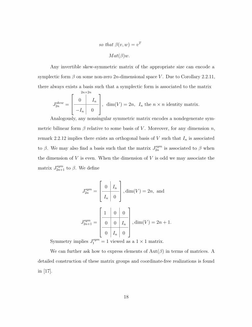
so that β(v, w) = vT

Mat(β)w.

Any invertible skew-symmetric matrix of the appropriate size can encode a

symplectic form β on some non-zero 2n-dimensional space V . Due to Corollary 2.2.11,

there always exists a basis such that a symplectic form is associated to the matrix

Jskew2n =

2n×2n 0 In

−In 0

, dim(V ) = 2n, In the n× n identity matrix.

Analogously, any nonsingular symmetric matrix encodes a nondegenerate sym-

metric bilinear form β relative to some basis of V . Moreover, for any dimension n,

remark 2.2.12 implies there exists an orthogonal basis of V such that In is associated

to β. We may also find a basis such that the matrix Jsym2n is associated to β when

the dimension of V is even. When the dimension of V is odd we may associate the

matrix Jsym2n+1 to β. We define

Jsym2n =

0 In

In 0

, dim(V ) = 2n, and

Jsym2n+1 =

1 0 0

0 0 In

0 In 0

, dim(V ) = 2n+ 1.

Symmetry implies Jsym1 = 1 viewed as a 1× 1 matrix.

We can further ask how to express elements of Aut(β) in terms of matrices. A

detailed construction of these matrix groups and coordinate-free realizations is found

in [17].

18

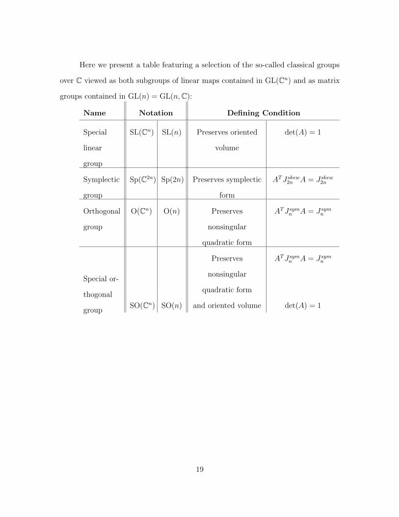
Here we present a table featuring a selection of the so-called classical groups

over C viewed as both subgroups of linear maps contained in GL(Cn) and as matrix

groups contained in GL(n) = GL(n,C):

Name Notation Defining Condition

Special

linear

group

SL(Cn) SL(n) Preserves oriented

volume

det(A) = 1

Symplectic

group

Sp(C2n) Sp(2n) Preserves symplectic

form

ATJskew2n A = Jskew2n

Orthogonal

group

O(Cn) O(n) Preserves

nonsingular

quadratic form

ATJsymn A = Jsymn

Special or-

thogonal

group

Preserves

nonsingular

quadratic form

ATJsymn A = Jsymn

SO(Cn) SO(n) and oriented volume det(A) = 1

19

CHAPTER 3

Algebras

A peculiar case: There is a word derived from the Arabic for “reunion of broken

parts” whose mathematical usage is attributed to Muhammed ibn Musa al-Khwarizmi.

This word algebra is found in many a course title from grammar/secondary school’s

Algebras I & II to College Algebra, from Linear Algebra to Abstract Algebra. With so

many appearances one hesitantly stumbles upon the question titling Section 1 of [37]:

“What is Algebra?” The answer therein describes a broader view of scientific pursuit as

we attempt to measure the world around us. The same text shows the term algebra

also has place amongst the definitions of Chapter 2 as a set with certain structure, as

an object describing transformation of space. Indeed, an algebra over a commutative

ring is essentially a module with its own multiplication compatible with the action

of the ring, i.e., r(mn) = (m)rn = rm(n), for r a ring element and m,n module

elements. The multiplication can be non-associative, associative, commutative, carry

a multiplicative identity, etc., giving rise to non-associative algebras, associative

algebras, commutative algebras, unital algebras, etc., respectively. A first walk

through a graduate algebra course may even describe an algebra via maps of rings to

the surprise of the student fixed on set-axiomatic descriptions of algebraic objects.

From a categorical point of view, groups, rings, vector spaces, and many more

structures are well-defined and well-explained through maps, the objects and arrows

between them [as in, e.g., 33]. In this chapter we shall define specific algebras of

interest and hint at the functorial nature involved in constructing algebras from vector

20

spaces. Beyond here, the reader is encouraged to explore the mathematical object,

scientific subfield of study, and philosophical perspective that is algebra.

First we make clear the definition of an associative unital algebra over C and a

map of such algebras.

Definition 3.0.1. Suppose f : C → A is a map of commutative unital rings such

that the image of f is contained in Z(A). Then we say A is a C-algebra by which we

mean an associative unital complex algebra.

The condition that f(C) ⊂ Z(A), recalling example 2.1.22, implies A is a vector

space over C. Naturally, a map of algebras is required to be both a linear map and a

map of rings.

There are various associative unital algebras associated with a vector space V .

3.1 Algebra of Endomorphisms and Free Algebras

In Chapter 2 we introduced the ring End(V ) while considering the abelian

group structure on V . The vector space End(V ) of linear maps also has an associative

product through function composition with 1V as the unit. That means we can view

End(V ) as an associative unital algebra. Following the proof of Proposition 2.2.14,

we have End(V ) is isomorphic to Mat(n) as algebras and dim(End(V )) = n2 when V

has finite dimension n.

Remark 3.1.1. The set End(V ) will continue to be a primary example to exhibit

various algebraic structures. Already we have seen End(V ) as a group, ring, vector

space, and algebra. Any associative algebra is certainly a group, ring, and vector

space, so there are no surprises here. Furthermore, an abstract algebra A acts on a

vector space V through algebra maps A→ End(V ).

Let V be the infinite-dimensional vector space of complex polynomials C[x1, . . . , xn]

in n indeterminates. We will be interested in an algebra A such that V is an A-

21

representation; equivalently, we will seek certain maps A→ End(V ) such that the

elements of A act on polynomials, a welcome sight to mathematicians. Some particu-

lar algebras A with V as a representation space arise from quotients of free algebras

generated by elements from End(V ). The ideals in the quotients will reflect the

relations on the elements present in the endomorphism ring. We give the definitions

needed below.

For any set X we define the free algebra C〈X〉 on X.

Definition 3.1.2. The free algebra C〈X〉 on X consists of all finite sums of words

w = αwk11 · · ·wkmm , α ∈ C, m ∈ N, wi ∈ X, ki ∈ N, 1 ≤ i ≤ m. By convention, the

empty word (α = 1, m = 0) is the multiplicative identity.

Definition 3.1.3. If C〈X〉 = C〈Y 〉 for a finite set Y , then C〈X〉 = C〈Y 〉 is called a

finitely-generated (free) algebra.

The construction above will be of particular use when X is a basis of a finite-

dimensional vector space V .

Remark 3.1.4. An ideal J of an associative algebra A is taken to be an ideal of the

ring structure of A.

Again consider V = C[x1, . . . , xn]. Consider the endomorphisms Pi : f 7→ xif

and Qi : f 7→ ∂f∂xi, 1 ≤ i ≤ n. Let X = Pi, Qi | 1 ≤ i ≤ n ⊂ End(V ). Then we

have the following relations on X

PiPj − PjPi = 0, 1 ≤ i, j ≤ n

QiQj −QjQi = 0, 1 ≤ i, j ≤ n

QiPj − PjQi = δij1V , 1 ≤ i, j ≤ n.

Then D(n) is the nth Weyl algebra of polynomial differential operators on

C[x1, . . . , xn] as the quotient C〈Pi, Qi | 1 ≤ i ≤ n〉J, where J is the ideal gener-

22

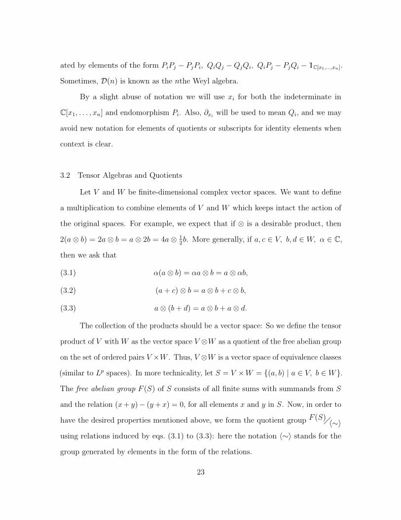
ated by elements of the form PiPj − PjPi, QiQj −QjQi, QiPj − PjQi − 1C[x1,...,xn].

Sometimes, D(n) is known as the nthe Weyl algebra.

By a slight abuse of notation we will use xi for both the indeterminate in

C[x1, . . . , xn] and endomorphism Pi. Also, ∂xi will be used to mean Qi, and we may

avoid new notation for elements of quotients or subscripts for identity elements when

context is clear.

3.2 Tensor Algebras and Quotients

Let V and W be finite-dimensional complex vector spaces. We want to define

a multiplication to combine elements of V and W which keeps intact the action of

the original spaces. For example, we expect that if ⊗ is a desirable product, then

2(a⊗ b) = 2a⊗ b = a⊗ 2b = 4a⊗ 12b. More generally, if a, c ∈ V, b, d ∈ W, α ∈ C,

then we ask that

α(a⊗ b) = αa⊗ b = a⊗ αb,(3.1)

(a+ c)⊗ b = a⊗ b+ c⊗ b,(3.2)

a⊗ (b+ d) = a⊗ b+ a⊗ d.(3.3)

The collection of the products should be a vector space: So we define the tensor

product of V with W as the vector space V ⊗W as a quotient of the free abelian group

on the set of ordered pairs V ×W . Thus, V ⊗W is a vector space of equivalence classes

(similar to Lp spaces). In more technicality, let S = V ×W = (a, b) | a ∈ V, b ∈ W.

The free abelian group F (S) of S consists of all finite sums with summands from S

and the relation (x+ y)− (y+ x) = 0, for all elements x and y in S. Now, in order to

have the desired properties mentioned above, we form the quotient group F (S)〈∼〉using relations induced by eqs. (3.1) to (3.3): here the notation 〈∼〉 stands for the

group generated by elements in the form of the relations.

23

The details of the construction using noncommutative rings and modules are in

[Chapter 4 of 22, Section 5]. As the factors of the tensor product do not have to be

the same vector space we can form the tensor products (V ⊗V )⊗V and V ⊗ (V ⊗V ).

Proposition 3.2.1. Let U, V,W be vector spaces. The vector spae (U ⊗ V )⊗W is

isomorphic to U ⊗ (V ⊗W ). Thus, we write U ⊗ V ⊗W without concern for the

parentheses, i.e., the tensor product is associative.

Proposition 3.2.2. If BV is basis for V and BW a basis for W , then bV ⊗bW | bV ∈

BV , bW ∈ BW is a basis for V ⊗W .

With Proposition 3.2.1 and Proposition 3.2.2 we are ready to define the tensor

algebra on V .

Definition 3.2.3. The kth tensor power of V is

T k(V ) = V ⊗ V ⊗ · · · ⊗ V︸ ︷︷ ︸k factors

,

with T 0(V ) = C and T 1(V ) = V . Elements of the vector space T k(V ) are called

k-tensors.

Definition 3.2.4. The tensor algebra T (V ) on V is the associative algebra

T (V ) =∞⊕k=0

T k(V ),

with associative product Tm(V ) ⊗ T n(V ) → Tm+n(V ) defined on m-tensors and

n-tensors by (vi1 ⊗ · · · ⊗ vim)⊗ (vj1 ⊗ · · · ⊗ vjn) = vi1 ⊗ · · · ⊗ vim ⊗ vj1 ⊗ · · · ⊗ vjn , and

extended by linearity.

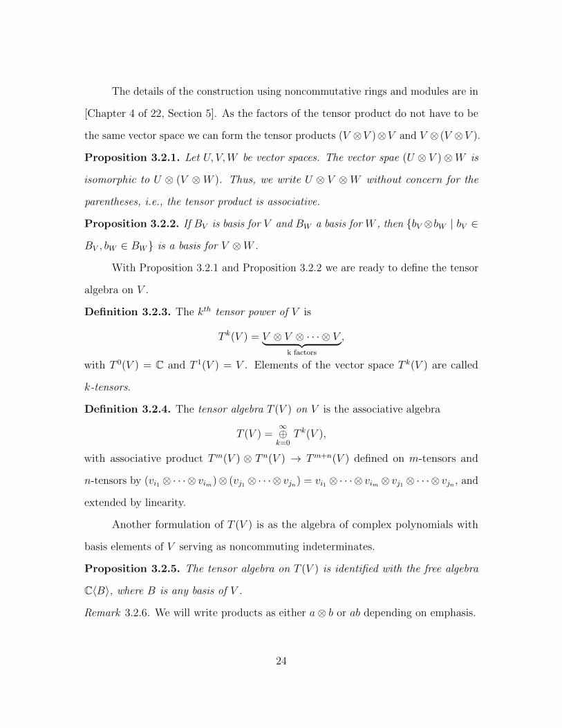
Another formulation of T (V ) is as the algebra of complex polynomials with

basis elements of V serving as noncommuting indeterminates.

Proposition 3.2.5. The tensor algebra on T (V ) is identified with the free algebra

C〈B〉, where B is any basis of V .

Remark 3.2.6. We will write products as either a⊗ b or ab depending on emphasis.

24

The algebra T (V ) is a coordinate-free realization of the free algebra associated

with V .

As mentioned, maps help define many algebraic objects. Universal properties

can also speak to the uniqueness of objects. In particular, we say the the tensor

algebra of V is a unique (up to isomorphism) associative algebra by the following

proposition:

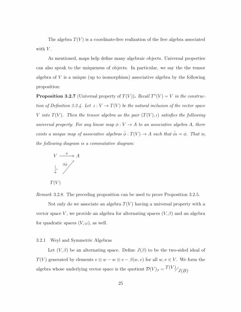
Proposition 3.2.7 (Universal property of T (V )). Recall T 1(V ) = V in the construc-

tion of Definition 3.2.4. Let ι : V → T (V ) be the natural inclusion of the vector space

V into T (V ). Then the tensor algebra as the pair (T (V ), ι) satisfies the following

universal property: For any linear map φ : V → A to an associative algebra A, there

exists a unique map of associative algebras φ : T (V )→ A such that φι = φ. That is,

the following diagram is a commutative diagram:

V A

T (V )

ι

φ

∃!φ

Remark 3.2.8. The preceding proposition can be used to prove Proposition 3.2.5.

Not only do we associate an algebra T (V ) having a universal property with a

vector space V , we provide an algebra for alternating spaces (V, β) and an algebra

for quadratic spaces (V, ω), as well.

3.2.1 Weyl and Symmetric Algebras

Let (V, β) be an alternating space. Define J(β) to be the two-sided ideal of

T (V ) generated by elements v ⊗ w − w ⊗ v − β(w, v) for all w, v ∈ V . We form the

algebra whose underlying vector space is the quotient D(V )β = T (V )J(B).

25

Definition 3.2.9. In the case β is a symplectic form, Corollary 2.2.11 tells us that

the dimension of V determines β. With the dimension of V equal to 2n, we define

the nth Weyl algebra D(n) = D(V )β.

Definition 3.2.10. When β is null we define the symmetric algebra S(V ) = D(V )β.

Remark 3.2.11. In light of Proposition 3.2.5, the algebra of polynomial differential

operators D(n) and the nth Weyl algebra D(n) are isomorphic. We use D(n) for both.

Furthermore, we view S(V ) as polynomials in V and S(V ∗) as polynomials on V .

Remark 3.2.12. Each of D(n) and S(V ) are associative unital algebras with universal

properties analogous to Proposition 3.2.7.

3.2.2 Clifford and Exterior Algebras

Let (V, ω) be a quadratic space. Define J(ω) to be the two-sided ideal of T (V )

generated by elements v⊗w+w⊗ v− ω(w, v) for all w, v ∈ V . We form the algebra

whose underlying vector space is the quotient C(V, β) = T (V )J(ω).

Definition 3.2.13. We call C(V, ω) the Clifford algebra of V associated with ω. If ω

is nonsingular, then we choose an orthogonal basis and speak of the Clifford algebra

Cl(V ) of V .

Definition 3.2.14. We define the exterior algebra∧

(V ) of V when ω is null.

Again, Proposition 3.2.5 gives us an isomorphism of algebras. We recognize∧V =

∧(V ) as anti-commuting polynomials C[ξ1, . . . , ξn] where ξ2

i = 0. The standard

way to express products in∧

(V ) is with the anti-commuting wedge: a ∧ b = −b ∧ a

with a ∧ a = 0.

Remark 3.2.15. Each of Cl(V ) and∧

(V ) are associative unital algebras with universal

properties analogous to Proposition 3.2.7.

26

3.3 Non-associative Algebras & Universal Enveloping Algebras

Non-associative algebras do exist! We give a complex vector space g a product

generalizing the properties of the pair (R3,×), real 3-space with the cross product.

Definition 3.3.1. A Lie algebra is a pair (g, [ , ]) such that [·, ·] : g × g → g is a

bilinear product (called the Lie bracket) on g and the following properties hold for all

vectors x, y, z ∈ g.

[x, y] = −[y, x].(3.4)

[x, [y, z]] = [[x, y], z] + [y, [x, z]].(3.5)

Remark 3.3.2. Abstract Lie algebras can be defined over commutative rings. Also,

requiring alternativity, [x, x] = 0, ∀x ∈ g, replaces eq. (3.4). Over C there is no

difference in assumptions.

Texts such as [17, 39] introduce Lie algebras through the connection with Lie

groups and the geometry of matrix groups. We take the more algebraic approach of

[10, 21] and give some standard examples before providing the “superized” definitions

in Chapter 4 needed for the main results.

3.3.1 Lie algebras

The set End(V ) serves as an example of a Lie algebra when paired with the

commutator as the bracket. It will be given a particular name and feature prominently

in the representation theoretic aspects of this work.

Remark 3.3.3. Any associative algebra with the commutator is a Lie algebra. Note

that the associativity of the multiplication in End(V ) is lacking in the Lie bracket

that is the commutator.

Definition 3.3.4. The general linear Lie algebra gl(V ) is the pair (End(V ), [ , ])

where [X, Y ] = XY − Y X is the commutator on endomorphisms X, Y .

27

Definition 3.3.5. The general linear Lie algebra gl(n) of rank n is the pair (Mat(n), [ , ])

where [A,B] = AB −BA is the commutator on n× n matrices A,B.

As might be expected, gl(V ) and gl(n) are isomorphic Lie algebras when

dim(V ) = n <∞. We say two Lie algebras are isomorphic as Lie algebras if there

exists an invertible linear map of the underlying vector spaces that respects the

bracket of each Lie algebra. We clarify below:

Definition 3.3.6. Let (g, [ , ]g) and (h, [ , ]h) be two Lie algebras. A linear map

φ : g→ h is a homomorphism of Lie algebras if φ([x, y]g) = [φ(x), φ(y)]h, ∀x, y ∈ g.

Lie algebras are also algebraic objects whose elements can act on vector spaces

as linear transformations. Precisely, the most important map of Lie algebras will

be those of the form g→ End(V ) for some Lie algebra g and some vector space V

serving as a representation space.

We continue with a list of definitions before a table of important examples.

Definition 3.3.7. A Lie subalgebra of a Lie algebra g is a subspace h ⊂ g such that

h is closed under the bracket: [h, h] ⊂ h. Without hesitation, we will refer to Lie

subalgebras as subalgebras.

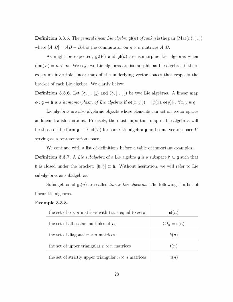
Subalgebras of gl(n) are called linear Lie algebras. The following is a list of

linear Lie algebras.

Example 3.3.8.

the set of n× n matrices with trace equal to zero sl(n)

the set of all scalar multiples of In CIn = s(n)

the set of diagonal n× n matrices d(n)

the set of upper triangular n× n matrices t(n)

the set of strictly upper triangular n× n matrices n(n)

28

Definition 3.3.9. An ideal of a Lie algebra is a subalgebra i ⊂ g such that [i, g] ⊂ g.

Example 3.3.10. Recall: tr (AB) = tr (BA) for any matrices A and B of size m×n

and n×m, respectively. From here we see sl(n) is an ideal of gl(n).

Definition 3.3.11. The center of a Lie algebra is the ideal Z(g) ⊂ g of elements

which give a trivial bracket when paired with any other element:

Z(g) = x ∈ g | [x, y] = 0, ∀y ∈ g. We call g an abelian Lie algebra when Z(g) = g.

Example 3.3.12. The center of gl(n) is s(n).

A non-abelian Lie algebra is called a simple Lie algebra if its only ideals are

itself and the zero subspace. A semisimple Lie algebra is the direct sum of simple

algebras where the bracket is trivial on distinct summands; hence, the algebras in the

summands are simple ideals.

Remark 3.3.13. Clearly, gl(n) is not simple, nor is it semisimple. Instead, gl(n) is a

reductive Lie algebra as the direct sum of a semisimple ideal sl(n) and its center s(n).

We emphasize that in gl(n) the center is the set of all elements commuting with

all others. This terminology of commuting elements is used also with abstract Lie

algebras.

Definition 3.3.14. Let g be a Lie algebra. The normalizer of a subalgebra h ⊂ g is

the subalgebra Ng(h) = x ∈ g | [x, h] ⊂ h.

A subalgebra is self-normalizing if Ng(h) = h.

Example 3.3.15. The diagonal matrices d(n) is a key example of a self-normalizing

algebra.

Definition 3.3.16. The derived algebra of a Lie algebra g is the ideal [g, g] ⊂ g

and defined to be the set span([x, y] | x, y ∈ g). In light of remark 3.3.13,

[gl(n), gl(n)] = sl(n).

29

The derived series of a Lie algebra g is the sequence of ideals g(0) = g, g(1) =

[g(0), g(0)], . . . , g(k) = [g(k−1), g(k−1)]. The lower central series of a Lie algebra g is the

sequence of ideals g0 = g, g1 = [g0, g0], . . . , gk = [gk−1, g].

Definition 3.3.17. A solvable Lie algebra is a Lie algebra g such that g(k) = 0 for

some k ∈ N0. We say g is a nilpotent Lie algebra if gk = 0 for some k ∈ N0. Nilpotent

algebras are solvable.

Example 3.3.18. The Lie algebras t(n) and n(n) are solvable. Indeed, n(n) is

nilpotent.

The diagonal matrices d(n) is a Lie algebra that is both nilpotent and self-

normalizing within the parent algebra gl(n). Such a Lie algebra is called a Cartan

algebra. When Cartan algebras exist, they play an important role in the representation

theory of Lie algebras.

We now describe some families of Lie algebras akin to the classical groups of

Chapter 2. They are subalgebras of sl(n) and are simple in most cases. Together with

sl(n) they form four infinite series of linear Lie algebras called classical Lie algebras.

Remark 3.3.19. An explanation of the correspondence between so-called connected

Lie groups and linear Lie algebras through the exponential map and 1-parameter

subgroups is carefully detailed in [34, 36].

Remark 3.3.20. We can choose a Cartan algebra hg of each Lie algebra g ⊂ gl(m)

below as hg = d(m) ∩ g.

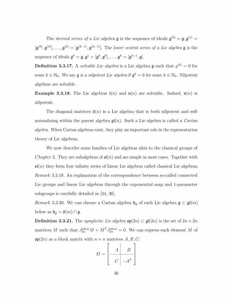
Definition 3.3.21. The symplectic Lie algebra sp(2n) ⊂ gl(2n) is the set of 2n× 2n

matrices M such that Jskew2n M +MTJskew2n = 0. We can express each element M of

sp(2n) as a block matrix with n× n matrices A,B,C:

M =

A B

C −AT

30

where B and C are symmetric matrices.

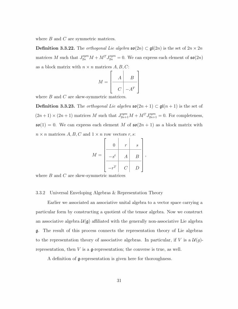
Definition 3.3.22. The orthogonal Lie algebra so(2n) ⊂ gl(2n) is the set of 2n× 2n

matrices M such that Jsym2n M +MTJsym2n = 0. We can express each element of so(2n)

as a block matrix with n× n matrices A,B,C:

M =

A B

C −AT

where B and C are skew-symmetric matrices.

Definition 3.3.23. The orthogonal Lie algebra so(2n+ 1) ⊂ gl(n+ 1) is the set of

(2n+ 1)× (2n+ 1) matrices M such that Jsym2n+1M +MTJsym2n+1 = 0. For completeness,

so(1) = 0. We can express each element M of so(2n + 1) as a block matrix with

n× n matrices A,B,C and 1× n row vectors r, s:

M =

0 r s

−st A B

−rT C D

,where B and C are skew-symmetric matrices

3.3.2 Universal Enveloping Algebras & Representation Theory

Earlier we associated an associative unital algebra to a vector space carrying a

particular form by constructing a quotient of the tensor algebra. Now we construct

an associative algebra U(g) affiliated with the generally non-associative Lie algebra

g. The result of this process connects the representation theory of Lie algebras

to the representation theory of associative algebras. In particular, if V is a U(g)-

representation, then V is a g-representation; the converse is true, as well.

A definition of g-representation is given here for thoroughness.

31

Definition 3.3.24. A representation of a Lie algebra g is a Lie algebra map ρ : g→

gl(V ). We can also speak of the pair (ρ, V ) or V by itself as a g-representation.

Example 3.3.25. Let V be a vector space of dimension n. If g is a Lie subalgebra

of gl(V ), then the inclusion map ι: g → gl(V ) is the standard representation of g.

Normally, we refer to the vector space Cn as the standard representation g.

Definition 3.3.26. Given a Lie algebra (g, [ , ]) with some abstract Lie bracket,

form the quotient T (V )I, where I is the ideal generated by elements of the form

x⊗ y − y ⊗ x− [x, y]. In this case, we use the term universal enveloping algebra of g

for the quotient U(g) = T (V )I.

By the observation made in remark 3.3.3, we view U(g) as a Lie algebra with the

commutator as the Lie bracket. The relations of the embedded Lie algebra g remain

and are key in justifying the use of “universal” as seen in the following proposition.

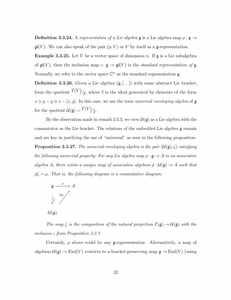
Proposition 3.3.27. The universal enveloping algebra is the pair (U(g), ζ) satisfying

the following universial property: For any Lie algebra map ρ : g→ A to an associative

algebra A, there exists a unique map of associative algebras ρ : U(g)→ A such that

ρζ = ρ. That is, the following diagram is a commutative diagram:

g A

U(g)

ζ

ρ

∃!ρ

The map ζ is the composition of the natural projection T (g)→ U(g) with the

inclusion ι from Proposition 3.2.7.

Certainly, ρ above could be any g-representation. Alternatively, a map of

algebras U(g)→ End(V ) restricts to a bracket-preserving map g→ End(V ) (using

32

the identification induced by ι). Then we have evidence to support the representation-

theoretic claims of the paragraph introducing this subsection.

The representations of a Lie algebra are also called g-modules, which seems to

make sense when considering U(g) is a ring and we now equate (left) modules of U(g)

with representations of g. Formally, a g-module is a vector space carrying a g-action

as described below:

Definition 3.3.28. Let V be a vector space and g a Lie algebra. Then V is a

module of g, more commonly, a g-module, when there is a well-defined g-action

g× V → V , (x, v)→ x.v, obeying

x.(v + w) = x.v + x.w, x ∈ g, v, w ∈ V(3.6)

(x+ y).(v) = x.v + y.v, x, y ∈ g, v ∈ V(3.7)

[x, y].v = x.(y.v)− y.(x.v), x, y ∈ g, v ∈ V.(3.8)

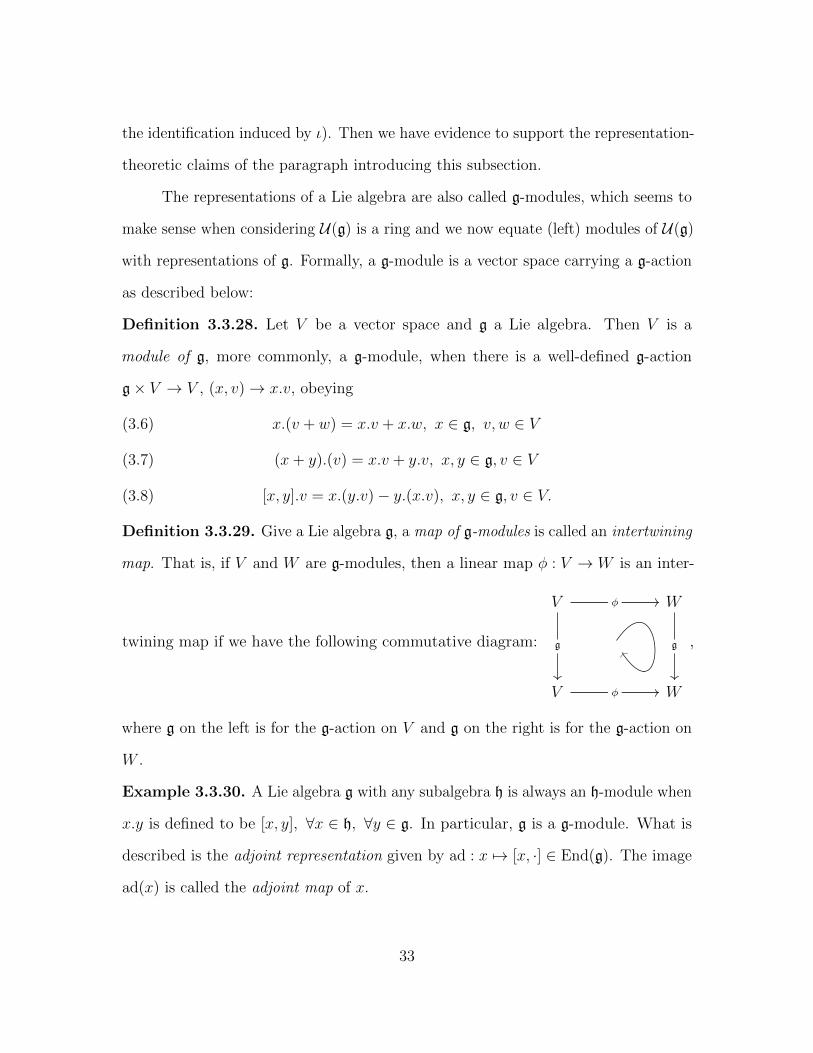
Definition 3.3.29. Give a Lie algebra g, a map of g-modules is called an intertwining

map. That is, if V and W are g-modules, then a linear map φ : V → W is an inter-

twining map if we have the following commutative diagram:

V W

V W

g

φ

g

φ

,

where g on the left is for the g-action on V and g on the right is for the g-action on

W .

Example 3.3.30. A Lie algebra g with any subalgebra h is always an h-module when

x.y is defined to be [x, y], ∀x ∈ h, ∀y ∈ g. In particular, g is a g-module. What is

described is the adjoint representation given by ad : x 7→ [x, ·] ∈ End(g). The image

ad(x) is called the adjoint map of x.

33

We give a detailed example of an intertwining map using g = sl(2), as the

concept will be crucial to future results.

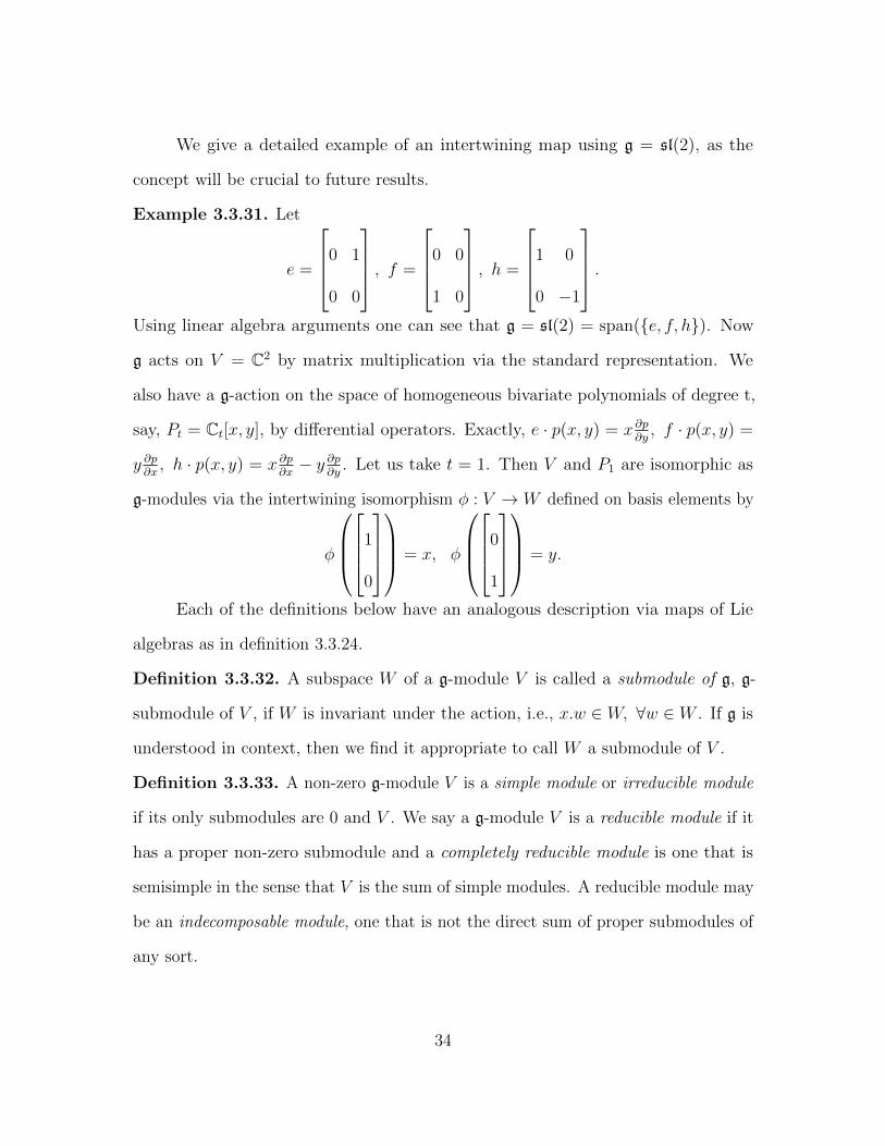
Example 3.3.31. Let

e =

0 1

0 0

, f =

0 0

1 0

, h =

1 0

0 −1

.Using linear algebra arguments one can see that g = sl(2) = span(e, f, h). Now

g acts on V = C2 by matrix multiplication via the standard representation. We

also have a g-action on the space of homogeneous bivariate polynomials of degree t,

say, Pt = Ct[x, y], by differential operators. Exactly, e · p(x, y) = x∂p∂y, f · p(x, y) =

y ∂p∂x, h · p(x, y) = x ∂p

∂x− y ∂p

∂y. Let us take t = 1. Then V and P1 are isomorphic as

g-modules via the intertwining isomorphism φ : V → W defined on basis elements by

φ

1

0

= x, φ

0

1

= y.

Each of the definitions below have an analogous description via maps of Lie

algebras as in definition 3.3.24.

Definition 3.3.32. A subspace W of a g-module V is called a submodule of g, g-

submodule of V , if W is invariant under the action, i.e., x.w ∈ W, ∀w ∈ W . If g is

understood in context, then we find it appropriate to call W a submodule of V .

Definition 3.3.33. A non-zero g-module V is a simple module or irreducible module

if its only submodules are 0 and V . We say a g-module V is a reducible module if it

has a proper non-zero submodule and a completely reducible module is one that is

semisimple in the sense that V is the sum of simple modules. A reducible module may

be an indecomposable module, one that is not the direct sum of proper submodules of

any sort.

34

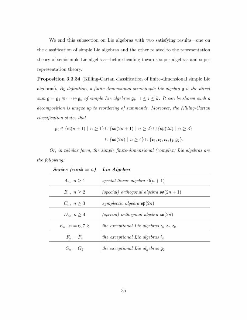
We end this subsection on Lie algebras with two satisfying results—one on

the classification of simple Lie algebras and the other related to the representation

theory of semisimple Lie algebras—before heading towards super algebras and super

representation theory.

Proposition 3.3.34 (Killing-Cartan classification of finite-dimensional simple Lie

algebras). By definition, a finite-dimensional semisimple Lie algebra g is the direct

sum g = g1 ⊕ · · · ⊕ gk of simple Lie algebras gi, 1 ≤ i ≤ k. It can be shown such a

decomposition is unique up to reordering of summands. Moreover, the Killing-Cartan

classification states that

gi ∈ sl(n+ 1) | n ≥ 1 ∪ so(2n+ 1) | n ≥ 2 ∪ sp(2n) | n ≥ 3

∪ so(2n) | n ≥ 4 ∪ e6, e7, e8, f4, g2.

Or, in tabular form, the simple finite-dimensional (complex) Lie algebras are

the following:

Series (rank = n) Lie Algebra

An, n ≥ 1 special linear algebra sl(n+ 1)

Bn, n ≥ 2 (special) orthogonal algebra so(2n+ 1)

Cn, n ≥ 3 symplectic algebra sp(2n)

Dn, n ≥ 4 (special) orthogonal algebra so(2n)

En, n = 6, 7, 8 the exceptional Lie algebras e6, e7, e8

Fn = F4 the exceptional Lie algebras f4

Gn = G2 the exceptional Lie algebras g2

35

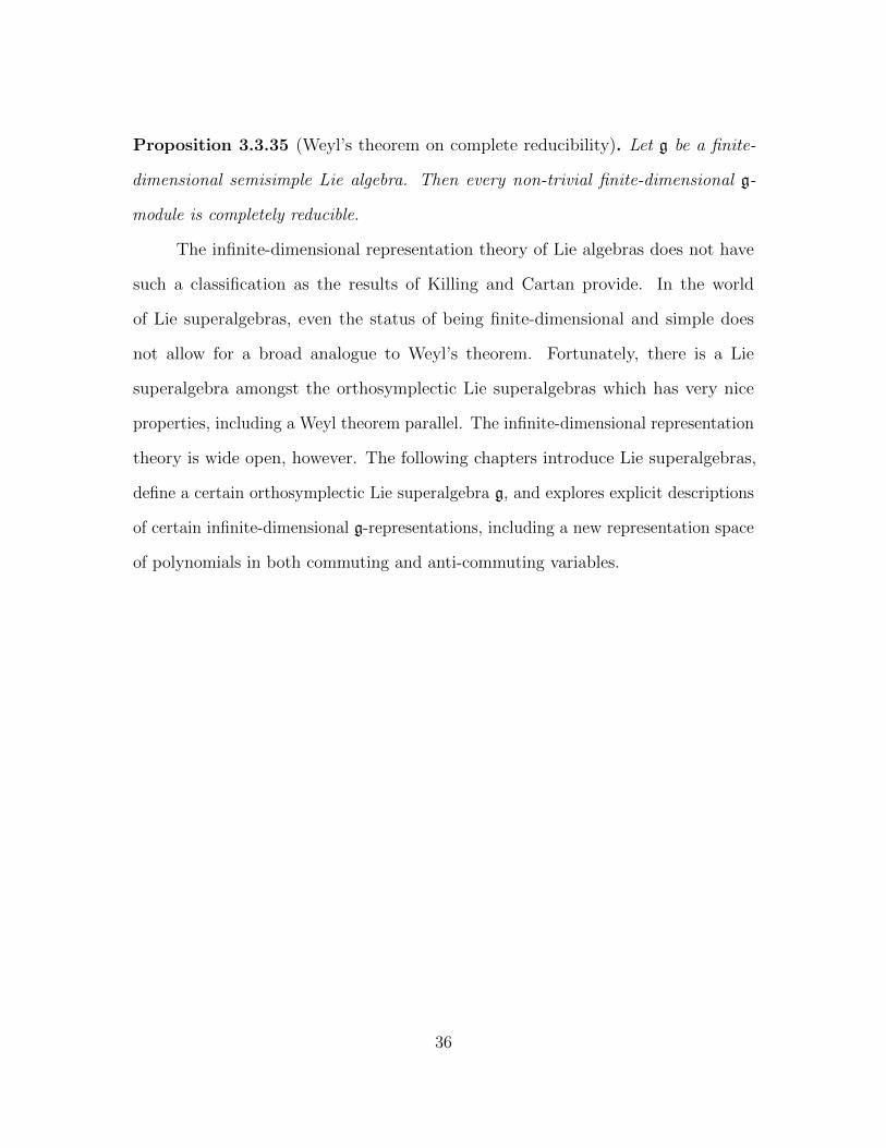
Proposition 3.3.35 (Weyl’s theorem on complete reducibility). Let g be a finite-

dimensional semisimple Lie algebra. Then every non-trivial finite-dimensional g-

module is completely reducible.

The infinite-dimensional representation theory of Lie algebras does not have

such a classification as the results of Killing and Cartan provide. In the world

of Lie superalgebras, even the status of being finite-dimensional and simple does

not allow for a broad analogue to Weyl’s theorem. Fortunately, there is a Lie

superalgebra amongst the orthosymplectic Lie superalgebras which has very nice

properties, including a Weyl theorem parallel. The infinite-dimensional representation

theory is wide open, however. The following chapters introduce Lie superalgebras,

define a certain orthosymplectic Lie superalgebra g, and explores explicit descriptions

of certain infinite-dimensional g-representations, including a new representation space

of polynomials in both commuting and anti-commuting variables.

36

CHAPTER 4

Superalgebras

While the goal of this work can be expressed in purely algebraic terms, and we

do tread an algebraic road, an exploration in algebra allows a picturesque view of

geometry, as well. The geometric connections are broad in application and conception.

One bridge between algebra and geometry is found in the aptly named area of algebraic

geometry, which relies on the tools of commutative algebra. Whereas the algebras

herein can be both noncommutative and non-associative, previous chapters described

vector spaces possessing some kind of geometry (certain bilinear spaces) affiliated with

Clifford and Weyl algebras, exterior and symmetric algebras, and classical Lie algebras,

few of which are commutative. Symplectic geometry begins with a symplectic form

as an element of the exterior algebra and involves (formal) Weyl algebras as another

example of the algebra-geometry link. Still, there are other concepts of geometry,

for example, noncommutative geometry [29] and supergeometry [30], arising from

beautiful mathematics and physical theories. These less-classical geometries rely on

the foundations of Hopf algebras [see 42] and the so-called quantum groups [29, again],

superalgebras, and Lie superalgebras. This chapter serves to develop a background in

superalgebras and Lie superalgebras and the prerequisite super Linear algebra to define

the extra structure on the underlying vector spaces. Here we encounter Z2-graded

vector spaces, often called super vector spaces1 or super spaces. The foundations

of Z2-graded vector spaces and general G-graded algebraic structures, where G a

1Technically, the symmetric monoidal category of super vector spaces has a different braidingthan that of the symmetric monoidal categroy of Z2-graded vector spaces.

37

monoid, preferably a commutative ring, is in [2, 28, 40]. Standard introductions to

Lie superalgebras include [5, 32]. We follow a similar course.

Throughout, we set Z2 to be Z2Z and denote the elements of Z2 by 0 and 1.

4.1 Super Linear Algebra

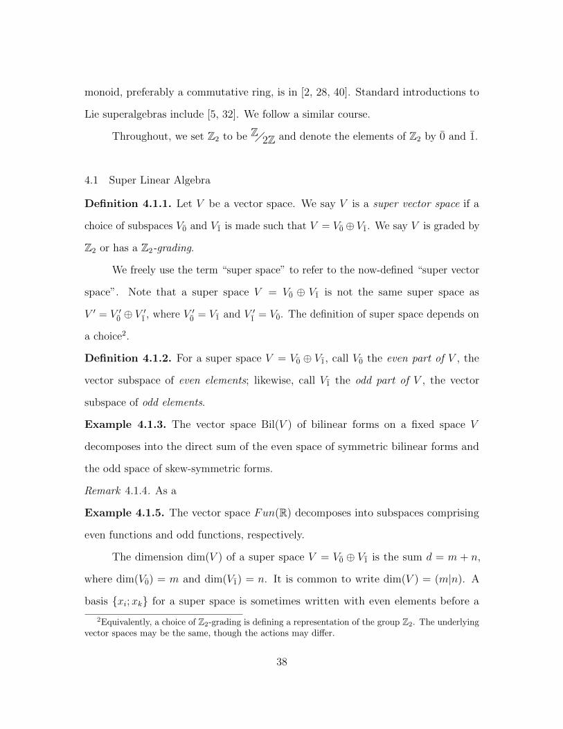
Definition 4.1.1. Let V be a vector space. We say V is a super vector space if a

choice of subspaces V0 and V1 is made such that V = V0 ⊕ V1. We say V is graded by

Z2 or has a Z2-grading.

We freely use the term “super space” to refer to the now-defined “super vector

space”. Note that a super space V = V0 ⊕ V1 is not the same super space as

V ′ = V ′0 ⊕ V′

1 , where V ′0 = V1 and V ′1 = V0. The definition of super space depends on

a choice2.

Definition 4.1.2. For a super space V = V0 ⊕ V1, call V0 the even part of V , the

vector subspace of even elements; likewise, call V1 the odd part of V , the vector

subspace of odd elements.

Example 4.1.3. The vector space Bil(V ) of bilinear forms on a fixed space V

decomposes into the direct sum of the even space of symmetric bilinear forms and

the odd space of skew-symmetric forms.

Remark 4.1.4. As a

Example 4.1.5. The vector space Fun(R) decomposes into subspaces comprising

even functions and odd functions, respectively.

The dimension dim(V ) of a super space V = V0 ⊕ V1 is the sum d = m + n,

where dim(V0) = m and dim(V1) = n. It is common to write dim(V ) = (m|n). A

basis xi;xk for a super space is sometimes written with even elements before a

2Equivalently, a choice of Z2-grading is defining a representation of the group Z2. The underlyingvector spaces may be the same, though the actions may differ.

38

semi-colon, with i ∈ I0, k ∈ I1, for some indexing set I = I0 t I1. We will often

suppress the semi-colon.

An important example of a super vector space is Cm|n = Cm ⊕ Cn.

Definition 4.1.6. Let V be a super space. Elements of V0tV1 are called homogeneous

elements of V .

Remark 4.1.7. Definition 4.1.6 provides a natural parity map p : V0 t V1 → Z2

(sometimes | · | : V0 t V1 → Z2) from homogeneous vectors of V to Z2. Indeed, the

use of p(x) implies x is homogeneous, while a homogeneous element xi may carry a

subscript for emphasis.

More generally, we can defined the degree of a homogeneous element in a G-

graded space, where G is a monoid. For example, V =⊕i∈N0

Vi, with Vi = spanC(xi)

is the N-graded vector space we recognize as the complex polynomials in one indeter-

minate. The degree map deg is defined on homogeneous elements by deg(x) = i for

x ∈ Vi. A Z-graded space of V is quickly made by setting Vi = 0, whenever i < 0.

Remark 4.1.8. Let V =⊕i∈ZVi be a Z-graded vector space. Then we have at least one

natural Z2-grading from the Z-grading by making V0 =⊕i∈2Z

Vi and V1 =⊕

i∈2Z+1

Vi.

Taking zero to be simultaneously even with parity 0 and odd with parity 1

has no adverse effects; similarly, zero can have any degree, and sometimes it is not

defined.

Definition 4.1.9. A map of super spaces φ : V → W is a parity-preserving map. In

particular, for every x0 + x1 = x ∈ V , φ(x) = φ(x0) + φ(x1), with φ(xi) ∈ Wi, i ∈ Z2.

A parity-reversing map φ is one where φ(xi) ∈ Wi+1, for all homogeneous xi.

Proposition 4.1.10. If V and W are super spaces and φ : V → W is linear, then

there exists a unique pair (φ0, φ1) of linear maps such that φ = φ0 + φ1, the map φ0

is parity-preserving, and the map φ1 is parity-reversing.

39

Proof. Suppose φ : V → W is a linear map with V = V0 + V1 and W = W0 +W1.

Choose a basis BV = xi;xk for V and a basis BW = yj; yl for W, with x ∈ B. If

φ(x) =m∑j=1

αjyj +n∑l=1

λlyl, then define φ0 and φ1 by

φ(x)0 =

m∑j=1

αjyj, if x is even

n∑l=1

λlyl, if x is odd

φ(x)1 =

n∑l=1

λlyl, if x is even

m∑j=1

αjyj, if x is odd.

Extend by linearity.

Corollary 4.1.11. For a super space V , the vector space End(V ) is a super space,

as well.

Remark 4.1.12. We will rely on Corollary 4.1.11 as, again, End(V ) plays a key role in

representation theory. Note that the space End(V )0 consists of exactly the maps φ

on the super space V .

Definition 4.1.13. A super subspace V of W = W0⊕W1 is a super space V = V0⊕V1

such that Vi ⊂ Wi, i ∈ Z2.

4.2 Lie Superalgebras

Many of the definitions below will be near-familiar as analogues of those found

in Section 3.3.1.

40

Definition 4.2.1. Let g = g0 ⊕ g1 be a superspace. A Lie superalgebra is a pair

(g, [ , ]) such that [·, ·] : g× g→ g is a bilinear product (called the Lie superbracket)

on g and the following properties hold for all homogeneous vectors x, y, z ∈ g.

[gi, gj] ⊂ gi+j, ∀i, j ∈ Z2(4.1)

[x, y] = −(−1)p(x)p(y)[y, x](4.2)

[x, [y, z]] = [[x, y], z] + (−1)p(x)p(y)[y, [x, z]].(4.3)

Equation (4.1) means the Lie superbracket is a parity-respecting product; Equation (4.2)

is the equation defining super skew-symmetry; and, Equation (4.3) is the super Jacobi

identity.

Remark 4.2.2. It should be clear that any vector space g has a trivial decomposition

g = g⊕0 as a super space. Moreover, a trivial Lie (super)bracket exists in all cases,

and, in the case g is a Lie algebra, then g has the structure of a Lie superalgebra

using the original Lie bracket.

Definition 4.2.3. Lie subsuperalgebras h are super subspaces of a Lie superalgebra

g such that h is closed under the Lie superbracket.

Definition 4.2.4. A map of Lie superalgebras φ : g → h is parity-preserving map

that is linear and bracket-preserving as in definition 3.3.1. We define isomorphisms

similarly.

Definition 4.2.5. Let X be a subset of a Lie superalgebra g. The Lie subsuperalgebra

〈X〉g generated by X is the span of all Lie superbrackets

〈X〉g =

n∑i=1

αiyi

∣∣∣∣∣ yi = [x1, [x2, ...[xk, xk+1]...]], xi ∈ X, αi ∈ C, k, n ∈ N

.

We say that a set X generates a Lie superalgebra g if 〈X〉g = g. If X is finite

then g is a finitely-generated Lie superalgebra. The empty set generates the zero Lie

superalgebra.

41

Proposition 4.2.6. Let g = 〈X〉g and h be Lie superalgebras with a map of super-

spaces φ : g→ h. Then φ is a map of Lie superalgebras if φ preserves the brackets on

generators x ∈ X. That is, φ([x, y]g) = [φ(x), φ(y)]h for all generators x, y ∈ X.

4.2.1 The general linear Lie superalgebra

Let V be a super space. The ubiquity of End(V ) emerges once more.

Definition 4.2.7. The general linear Lie superalgebra gl(V ) is the pair (End(V ), [ , ])

where [X, Y ] = (−1)p(X)p(Y )XY − Y X is the supercommutator on homogeneous

endomorphisms X, Y .

If a vector space V has dimension m+n, then we know End(V ) and End(m+n)

are isomorphic vector spaces. For similar reasons, the Lie superalgebra End(V ) is

isomorphic to gl(m|n), which is defined below.

Definition 4.2.8. The Lie superalgebra gl(m|n) consists of block matrices

X =

A B

C D

,where A ∈ Mat(m) and D ∈ Mat(n). The even matrices are those block matrices X

with B = C = 0, while the odd matrices have A = D = 0.

The even part gl(m|n)0 of gl(m|n) is isomorphic to the direct sum glm ⊕ gln of

two general linear Lie algebras.

Remark 4.2.9. The even part g0 of a Lie superalgebra g is a Lie algebra with Lie

bracket taken to be the superbracket restricted to g0.

The Lie superalgebra analogue of sl(n) is the Lie superalgebra sl(m|n) consisting

of all block matrices X =

A B

C D

in gl(m|n) such that str (X) = 0, where the

supertrace str (X) of X is equal to tr (A)− tr (D).

42

For matrix Lie superalgebras, we can choose a subset B ⊂ Eij of elementary

matrices as a basis.

Proposition 4.2.10. The Lie superbracket is defined on basis elements of gl(m|n)

as follows:

[Eij, Ekl] = δjkEil − (−1)p(Eij)p(Ekl)δilEkj.

4.2.2 Modules of Lie superalgebras

Representations of a Lie algebra g and g-modules are equivalent. The same

holds for Lie superalgebras, and we will move to using the term “module” more so

than “representation” for the sake of reading consistency. In this subsection, we

provide a few definitions of supermodules. The reader is encouraged to employ a

super version of the module theory, including examples, found in Section 3.3.2.

Definition 4.2.11. Let V = V0⊕V1 be a super vector space and g a Lie superalgebra.

Then V is a supermodule of g, more succinctly, a g-supermodule, when there is a

well-defined action g× V → V , (x, v)→ x.v, obeying

p(x.v) = p(x) + p(v) = i+ j, x ∈ gi, v ∈ Vj(4.4)

x.(v + w) = x.v + x.w, x ∈ g, v, w ∈ V(4.5)

(x+ y).(v) = x.v + y.v, x, y ∈ g, v ∈ V(4.6)

[x, y].v = x.(y.v)− (−1)p(x)p(y)y.(x.v), x, yx ∈ gi, v ∈ Vj(4.7)

Remark 4.2.12. Equation (4.4) ensures that the action of g on V is compatible with

the Z2-gradings of g and V .

Clearly, quotients of super spaces by super subspaces are again superspaces.

Definition 4.2.13. Let g be a Lie superalgebra with supermodules W ⊂ V . The

quotient module VW is the g-supermodule defined by x · (v +W ) = x.v +W, ∀v ∈

V, ∀x ∈ g.

43

4.3 Associative superalgebras

As in Chapter 3, we now establish a correspondence between the non-associative

Lie superalgebra g and an associative (super)algebra U(g). This universal enveloping

algebra U(g) will have a Z2-grading but does not require construction via a graded

tensor product of super vector spaces. Still, we provide a definition of a super tensor

product. We also relay a specific version of the celebrated PBW theorem which

provides a basis for U(g) when g has finite dimension. Lastly, the universal enveloping

algebra plays a part in determining the simplicity of a super module.

Definition 4.3.1. A complex associative unital superalgebra is a super vector space

A = A0⊕A1, with a bilinear parity-respecting product (a, b) 7→ ab ∈ A, for all a, b ∈ A.

That is, A = A0 ⊕A1 is an associative unital algebra with AiAj = Ai+j , for i, j ∈ Z2.

Remark 4.3.2. We have the super version of remark 3.3.3. Namely, any associative su-

peralgebra with the supercommutator, [x, y]=xy− (−1)p(x)p(y)yx, for all homogeneous

elements x and y, is a Lie superalgebra.

Definition 4.3.3. Let A and B be associative superalgebras. A map φ : A→ B is

a map of associative superalgebras if φ is a map of super spaces such that φ(xy) =

φ(x)φ(y), for all x, y ∈ A.

4.3.1 Universal enveloping algebras of Lie superalgebras

We appeal to a superization of Proposition 3.3.27.

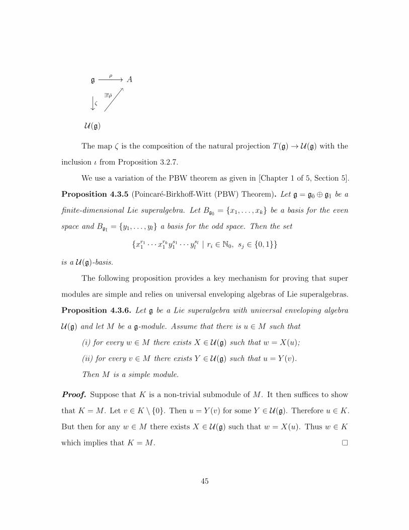
Definition 4.3.4. The universal enveloping algebra of a Lie superalgebra g is the pair

(U(g), ζ) satisfying the following universial property: For any Lie superalgebra map

ρ : g→ A to an associative superalgebra A, there exists a unique map of associative

superalgebras ρ : U(g) → A such that ρζ = ρ. That is, the following diagram is a

commutative diagram:

44

g A

U(g)

ζ

ρ

∃!ρ

The map ζ is the composition of the natural projection T (g)→ U(g) with the

inclusion ι from Proposition 3.2.7.

We use a variation of the PBW theorem as given in [Chapter 1 of 5, Section 5].

Proposition 4.3.5 (Poincare-Birkhoff-Witt (PBW) Theorem). Let g = g0 ⊕ g1 be a

finite-dimensional Lie superalgebra. Let Bg0= x1, . . . , xk be a basis for the even

space and Bg1= y1, . . . , yl a basis for the odd space. Then the set

xr11 · · ·xrk1 y

s11 · · · y

sll | ri ∈ N0, sj ∈ 0, 1

is a U(g)-basis.

The following proposition provides a key mechanism for proving that super

modules are simple and relies on universal enveloping algebras of Lie superalgebras.

Proposition 4.3.6. Let g be a Lie superalgebra with universal enveloping algebra

U(g) and let M be a g-module. Assume that there is u ∈M such that

(i) for every w ∈M there exists X ∈ U(g) such that w = X(u);

(ii) for every v ∈M there exists Y ∈ U(g) such that u = Y (v).

Then M is a simple module.

Proof. Suppose that K is a non-trivial submodule of M . It then suffices to show

that K = M . Let v ∈ K \ 0. Then u = Y (v) for some Y ∈ U(g). Therefore u ∈ K.

But then for any w ∈ M there exists X ∈ U(g) such that w = X(u). Thus w ∈ K

which implies that K = M .

45

Interestingly enough, we did not define the “super tensor algebra” in order

to define the universal enveloping algebra of a Lie superalgebra. Indeed, the tensor

algebra as normally constructed will be graded in the manner of remark 4.1.8 (and as

the Weyl superalgebra in the next subsection). Nevertheless, we define a particular

graded tensor product here.

Definition 4.3.7. The super tensor product V ⊗W on super spaces V and W is

the super space V ⊗W = (V ⊗W )0 ⊕ (V ⊗W )1, using the tensor product of vector

spaces, where

(V ⊗W )0 = (V0 ⊗W0)⊕ (V1 ⊗W1)(4.8)

(V ⊗W )1 = (V0 ⊗W1)⊕ (V1 ⊗W0).(4.9)

In particular, p(a⊗ b) = p(a) + p(b), for all tensors a⊗ b.

Remark 4.3.8. We could define a Z2-graded tensor product on Z2-graded vector spaces

in the exact same way. The subtlety3 appears in the tensor product of superalgebras

versus the tensor product of Z2-graded algebras. A tensor product of superalgebras

is again a superalgebra with a product extended from this definition on homogeneous

tensors: (a⊗ b)(c⊗ d) = (−1)p(b)p(c)ac⊗ bd. No such power of -1 is required in the

non-super, but Z2-graded, case.

4.4 Weyl superalgebras

We close the chapter describing the nth Weyl superalgebra.

Recall the nth Weyl algebra D(n) of Chapter 3. In particular, refer to section 3.1

to define D(n) as the algebra of polynomial differential operators whose underlying

vector space is the span of monomials

span(xi1 · · ·xik∂xj1 · · · ∂xjl | 1 < i1, . . . , ik, j1, . . . , jl ≤ n, k, l ∈ N0) ⊂ End(C[x1, . . . , xn]).

3The categorical approach/difference was hinted at in a footnote of this chapter’s introduction

46

To define parity on D(n), we establish a Z-grading of D(n) as follows. Set deg(xi) = 1

and deg(∂xi) = −1 before extending the degree map on D(n) multiplicatively. Namely,

deg(xi1 · · ·xik∂xj1 · · · ∂xjl ) =k∑r=1

ip −l∑

q=1

jq.

Now D(n) is an associative unital superalgebra by remark 4.1.8. We will use

D(n) to construct g-modules of certain Lie superalgebras introduced in the next

chapter.

47

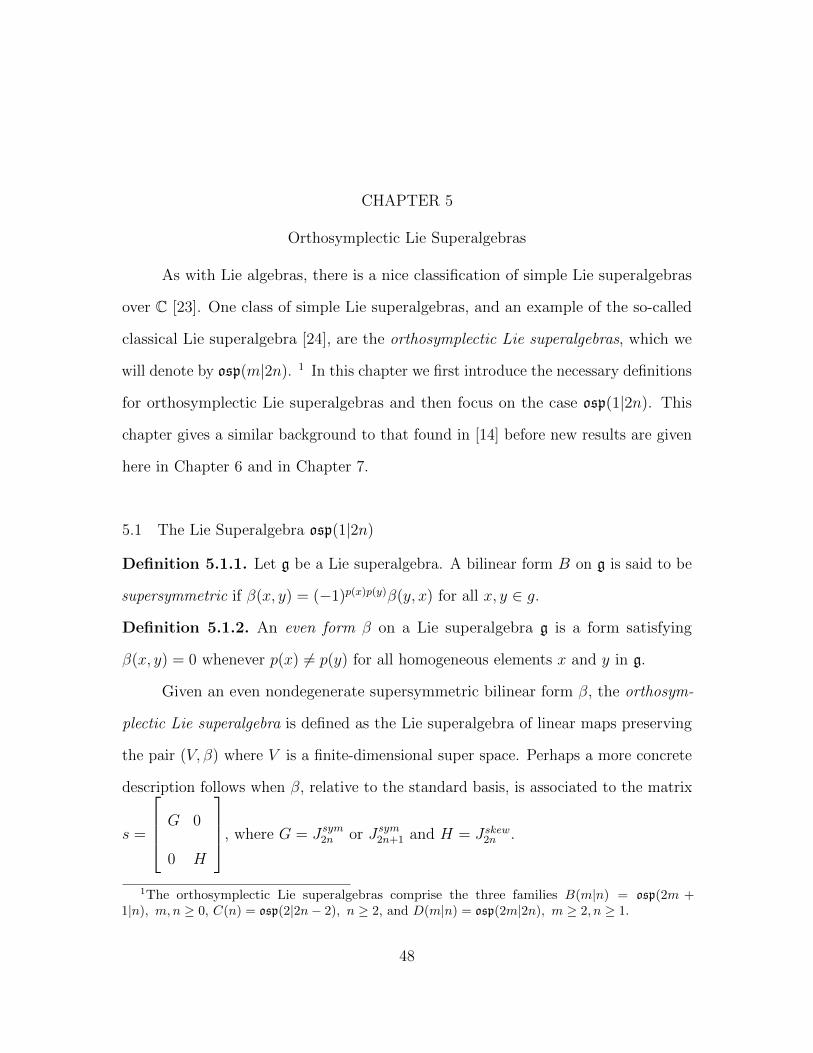
CHAPTER 5

Orthosymplectic Lie Superalgebras

As with Lie algebras, there is a nice classification of simple Lie superalgebras

over C [23]. One class of simple Lie superalgebras, and an example of the so-called

classical Lie superalgebra [24], are the orthosymplectic Lie superalgebras, which we

will denote by osp(m|2n). 1 In this chapter we first introduce the necessary definitions

for orthosymplectic Lie superalgebras and then focus on the case osp(1|2n). This

chapter gives a similar background to that found in [14] before new results are given

here in Chapter 6 and in Chapter 7.

5.1 The Lie Superalgebra osp(1|2n)

Definition 5.1.1. Let g be a Lie superalgebra. A bilinear form B on g is said to be

supersymmetric if β(x, y) = (−1)p(x)p(y)β(y, x) for all x, y ∈ g.

Definition 5.1.2. An even form β on a Lie superalgebra g is a form satisfying

β(x, y) = 0 whenever p(x) 6= p(y) for all homogeneous elements x and y in g.

Given an even nondegenerate supersymmetric bilinear form β, the orthosym-

plectic Lie superalgebra is defined as the Lie superalgebra of linear maps preserving

the pair (V, β) where V is a finite-dimensional super space. Perhaps a more concrete

description follows when β, relative to the standard basis, is associated to the matrix

s =

G 0

0 H

, where G = Jsym2n or Jsym2n+1 and H = Jskew2n .

1The orthosymplectic Lie superalgebras comprise the three families B(m|n) = osp(2m +1|n), m, n ≥ 0, C(n) = osp(2|2n− 2), n ≥ 2, and D(m|n) = osp(2m|2n), m ≥ 2, n ≥ 1.

48

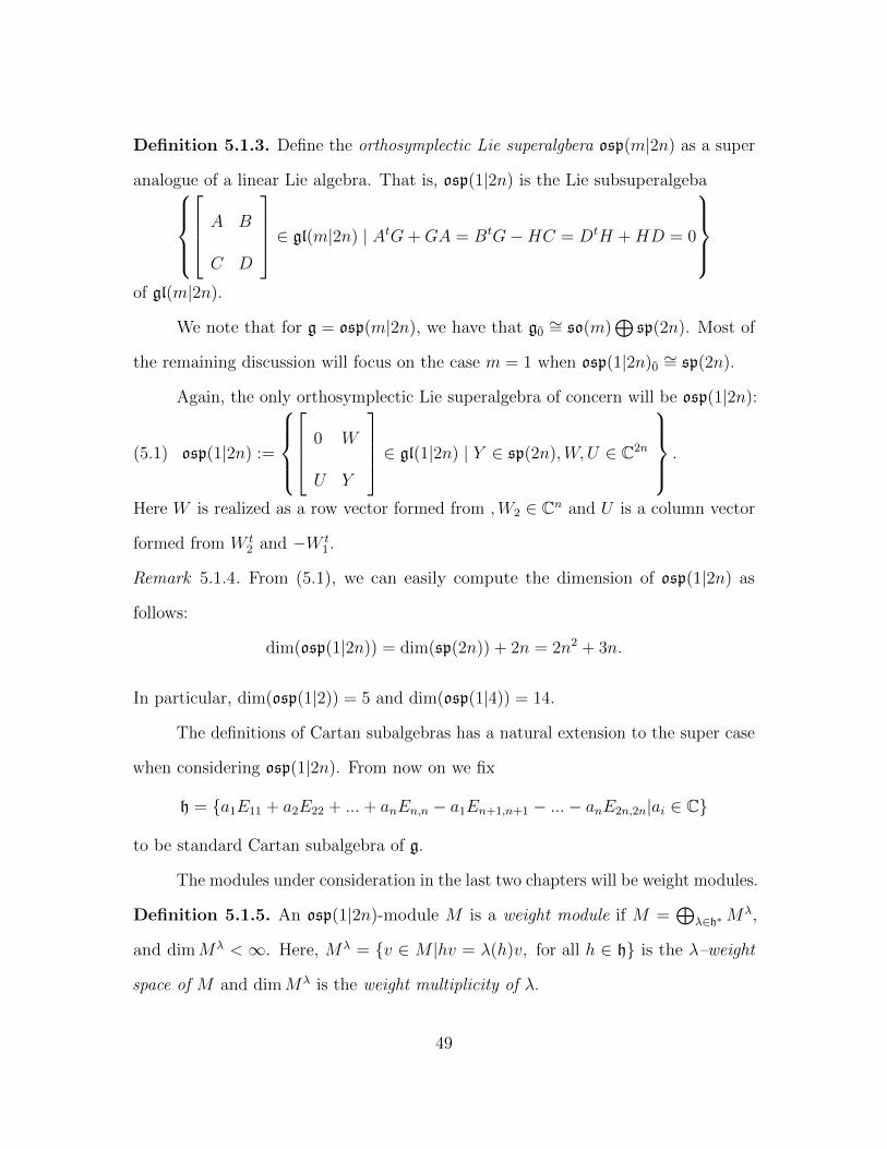
Definition 5.1.3. Define the orthosymplectic Lie superalgbera osp(m|2n) as a super

analogue of a linear Lie algebra. That is, osp(1|2n) is the Lie subsuperalgeba A B

C D

∈ gl(m|2n) | AtG+GA = BtG−HC = DtH +HD = 0

of gl(m|2n).

We note that for g = osp(m|2n), we have that g0∼= so(m)

⊕sp(2n). Most of

the remaining discussion will focus on the case m = 1 when osp(1|2n)0∼= sp(2n).

Again, the only orthosymplectic Lie superalgebra of concern will be osp(1|2n):

osp(1|2n) :=

0 W

U Y

∈ gl(1|2n) | Y ∈ sp(2n),W, U ∈ C2n

.(5.1)

Here W is realized as a row vector formed from ,W2 ∈ Cn and U is a column vector

formed from W t2 and −W t

1.

Remark 5.1.4. From (5.1), we can easily compute the dimension of osp(1|2n) as

follows:

dim(osp(1|2n)) = dim(sp(2n)) + 2n = 2n2 + 3n.

In particular, dim(osp(1|2)) = 5 and dim(osp(1|4)) = 14.

The definitions of Cartan subalgebras has a natural extension to the super case

when considering osp(1|2n). From now on we fix

h = a1E11 + a2E22 + ...+ anEn,n − a1En+1,n+1 − ...− anE2n,2n|ai ∈ C

to be standard Cartan subalgebra of g.

The modules under consideration in the last two chapters will be weight modules.

Definition 5.1.5. An osp(1|2n)-module M is a weight module if M =⊕

λ∈h∗Mλ,

and dimMλ < ∞. Here, Mλ = v ∈ M |hv = λ(h)v, for all h ∈ h is the λ–weight

space of M and dimMλ is the weight multiplicity of λ.

49

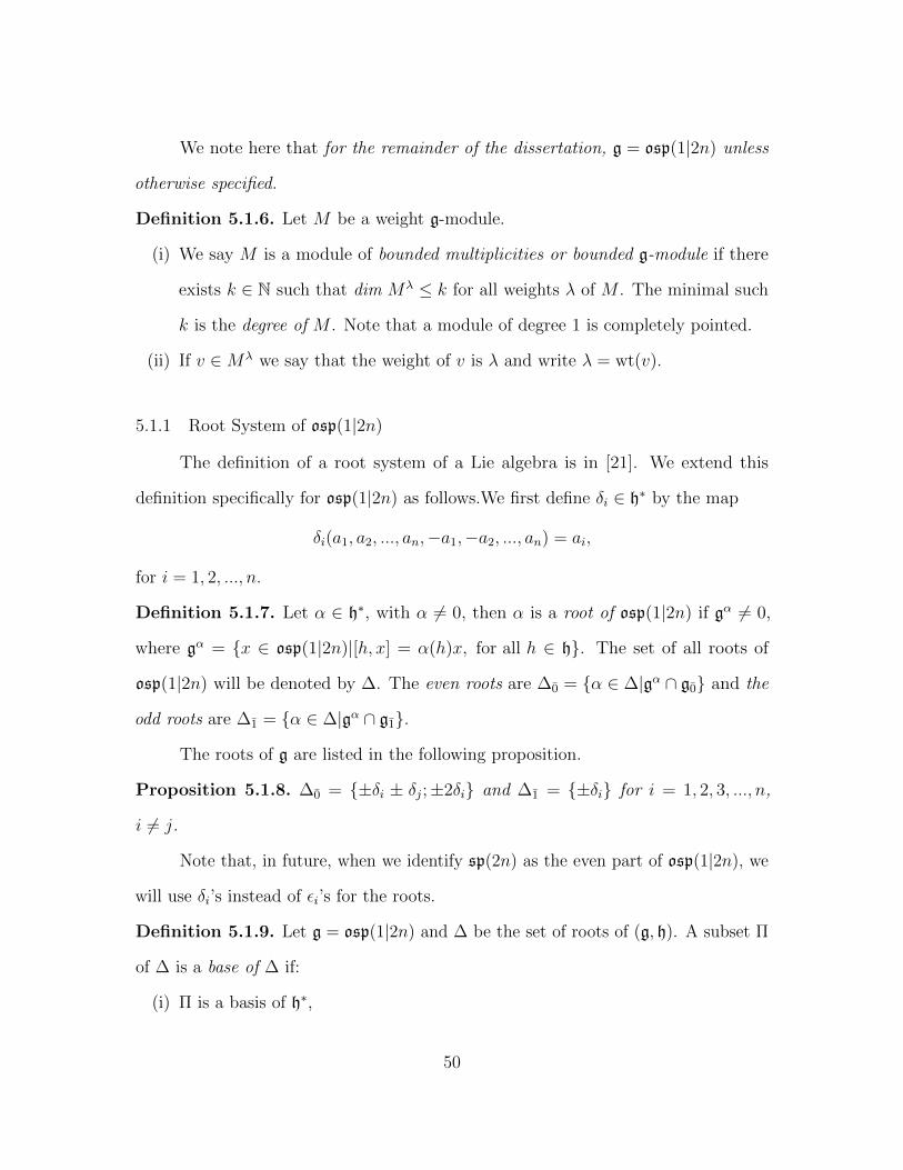
We note here that for the remainder of the dissertation, g = osp(1|2n) unless

otherwise specified.

Definition 5.1.6. Let M be a weight g-module.

(i) We say M is a module of bounded multiplicities or bounded g-module if there

exists k ∈ N such that dim Mλ ≤ k for all weights λ of M . The minimal such

k is the degree of M . Note that a module of degree 1 is completely pointed.

(ii) If v ∈Mλ we say that the weight of v is λ and write λ = wt(v).

5.1.1 Root System of osp(1|2n)

The definition of a root system of a Lie algebra is in [21]. We extend this

definition specifically for osp(1|2n) as follows.We first define δi ∈ h∗ by the map

δi(a1, a2, ..., an,−a1,−a2, ..., an) = ai,

for i = 1, 2, ..., n.

Definition 5.1.7. Let α ∈ h∗, with α 6= 0, then α is a root of osp(1|2n) if gα 6= 0,

where gα = x ∈ osp(1|2n)|[h, x] = α(h)x, for all h ∈ h. The set of all roots of

osp(1|2n) will be denoted by ∆. The even roots are ∆0 = α ∈ ∆|gα ∩ g0 and the

odd roots are ∆1 = α ∈ ∆|gα ∩ g1.

The roots of g are listed in the following proposition.

Proposition 5.1.8. ∆0 = ±δi ± δj;±2δi and ∆1 = ±δi for i = 1, 2, 3, ..., n,

i 6= j.

Note that, in future, when we identify sp(2n) as the even part of osp(1|2n), we

will use δi’s instead of εi’s for the roots.

Definition 5.1.9. Let g = osp(1|2n) and ∆ be the set of roots of (g, h). A subset Π

of ∆ is a base of ∆ if:

(i) Π is a basis of h∗,

50

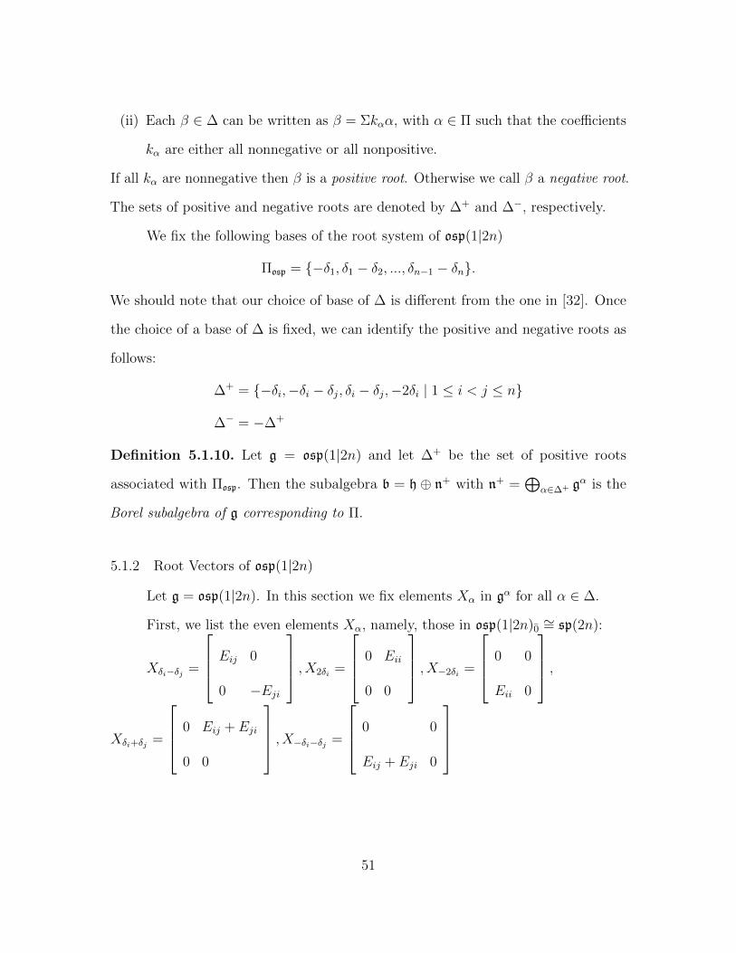
(ii) Each β ∈ ∆ can be written as β = Σkαα, with α ∈ Π such that the coefficients

kα are either all nonnegative or all nonpositive.

If all kα are nonnegative then β is a positive root. Otherwise we call β a negative root.

The sets of positive and negative roots are denoted by ∆+ and ∆−, respectively.

We fix the following bases of the root system of osp(1|2n)

Πosp = −δ1, δ1 − δ2, ..., δn−1 − δn.

We should note that our choice of base of ∆ is different from the one in [32]. Once

the choice of a base of ∆ is fixed, we can identify the positive and negative roots as

follows:

∆+ = −δi,−δi − δj, δi − δj,−2δi | 1 ≤ i < j ≤ n

∆− = −∆+

Definition 5.1.10. Let g = osp(1|2n) and let ∆+ be the set of positive roots

associated with Πosp. Then the subalgebra b = h⊕ n+ with n+ =⊕

α∈∆+ gα is the

Borel subalgebra of g corresponding to Π.

5.1.2 Root Vectors of osp(1|2n)

Let g = osp(1|2n). In this section we fix elements Xα in gα for all α ∈ ∆.

First, we list the even elements Xα, namely, those in osp(1|2n)0∼= sp(2n):

Xδi−δj =

Eij 0

0 −Eji

, X2δi =

0 Eii

0 0

, X−2δi =

0 0

Eii 0

,

Xδi+δj =

0 Eij + Eji

0 0

, X−δi−δj =

0 0

Eij + Eji 0

51

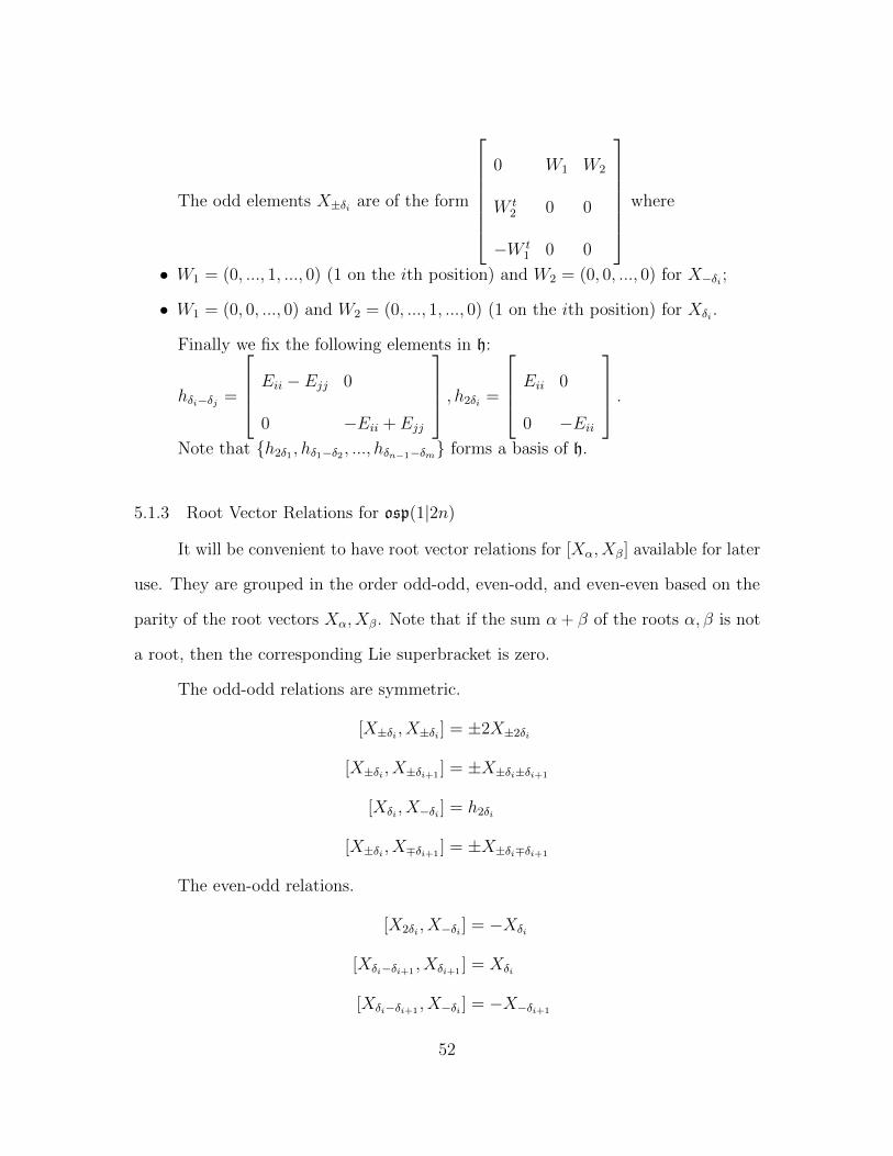
The odd elements X±δi are of the form

0 W1 W2

W t2 0 0

−W t1 0 0

where

• W1 = (0, ..., 1, ..., 0) (1 on the ith position) and W2 = (0, 0, ..., 0) for X−δi ;

• W1 = (0, 0, ..., 0) and W2 = (0, ..., 1, ..., 0) (1 on the ith position) for Xδi .

Finally we fix the following elements in h:

hδi−δj =

Eii − Ejj 0

0 −Eii + Ejj

, h2δi =

Eii 0

0 −Eii

.Note that h2δ1 , hδ1−δ2 , ..., hδn−1−δm forms a basis of h.

5.1.3 Root Vector Relations for osp(1|2n)

It will be convenient to have root vector relations for [Xα, Xβ] available for later

use. They are grouped in the order odd-odd, even-odd, and even-even based on the

parity of the root vectors Xα, Xβ. Note that if the sum α+ β of the roots α, β is not

a root, then the corresponding Lie superbracket is zero.

The odd-odd relations are symmetric.

[X±δi , X±δi ] = ±2X±2δi

[X±δi , X±δi+1] = ±X±δi±δi+1

[Xδi , X−δi ] = h2δi

[X±δi , X∓δi+1] = ±X±δi∓δi+1

The even-odd relations.

[X2δi , X−δi ] = −Xδi

[Xδi−δi+1, Xδi+1

] = Xδi

[Xδi−δi+1, X−δi ] = −X−δi+1

52

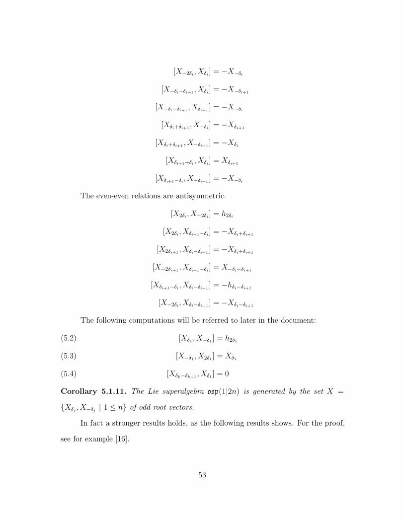
[X−2δi , Xδi ] = −X−δi

[X−δi−δi+1, Xδi ] = −X−δi+1

[X−δi−δi+1, Xδi+1

] = −X−δi

[Xδi+δi+1, X−δi ] = −Xδi+1

[Xδi+δi+1, X−δi+1

] = −Xδi

[Xδi+1+δi , Xδi ] = Xδi+1

[Xδi+1−δi , X−δi+1] = −X−δi

The even-even relations are antisymmetric.

[X2δi , X−2δi ] = h2δi

[X2δi , Xδi+1−δi ] = −Xδi+δi+1

[X2δi+1, Xδi−δi+1

] = −Xδi+δi+1

[X−2δi+1, Xδi+1−δi ] = X−δi−δi+1

[Xδi+1−δi , Xδi−δi+1] = −hδi−δi+1

[X−2δi , Xδi−δi+1] = −Xδi−δi+1

The following computations will be referred to later in the document:

[Xδ1 , X−δ1 ] = h2δ1(5.2)

[X−δ1 , X2δ1 ] = Xδ1(5.3)

[Xδk−δk+1, Xδ1 ] = 0(5.4)

Corollary 5.1.11. The Lie superalgebra osp(1|2n) is generated by the set X =

Xδj , X−δj | 1 ≤ n of odd root vectors.

In fact a stronger results holds, as the following results shows. For the proof,

see for example [16].

53

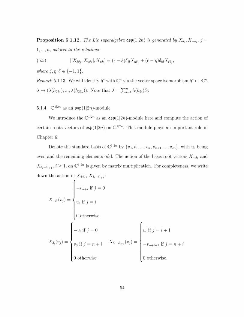
Proposition 5.1.12. The Lie superalgebra osp(1|2n) is generated by Xδj , X−δj , j =

1, ..., n, subject to the relations

(5.5) [[Xξδj , Xηδk ], Xεδl ] = (ε− ξ)δjlXηδk + (ε− η)δklXξδj ,

where ξ, η, δ ∈ −1, 1.

Remark 5.1.13. We will identify h∗ with Cn via the vector space isomorphism h∗ 7→ Cn,

λ 7→ (λ(h2δ1), ..., λ(h2δn)). Note that λ =∑n

i=1 λ(h2i)δi.

5.1.4 C1|2n as an osp(1|2n)-module

We introduce the C1|2n as an osp(1|2n)-module here and compute the action of

certain roots vectors of osp(1|2n) on C1|2n. This module plays an important role in

Chapter 6.

Denote the standard basis of C1|2n by v0, v1, ..., vn, vn+1, ..., v2n, with v0 being

even and the remaining elements odd. The action of the basis root vectors X−δ1 and

Xδi−δi+1, i ≥ 1, on C1|2n is given by matrix multiplication. For completeness, we write

down the action of X±δi , Xδi−δi+1:

X−δi(vj) =

−vn+i if j = 0

v0 if j = i

0 otherwise

Xδi(vj) =

−vi if j = 0

v0 if j = n+ i

0 otherwise

Xδi−δi+1(vj) =

vi if j = i+ 1

−vn+i+1 if j = n+ i

0 otherwise.

54

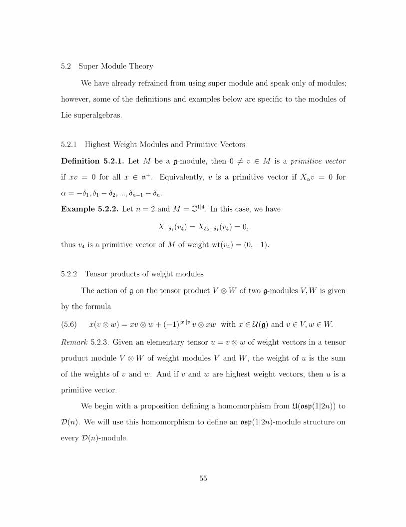
5.2 Super Module Theory

We have already refrained from using super module and speak only of modules;

however, some of the definitions and examples below are specific to the modules of

Lie superalgebras.

5.2.1 Highest Weight Modules and Primitive Vectors

Definition 5.2.1. Let M be a g-module, then 0 6= v ∈ M is a primitive vector

if xv = 0 for all x ∈ n+. Equivalently, v is a primitive vector if Xαv = 0 for

α = −δ1, δ1 − δ2, ..., δn−1 − δn.

Example 5.2.2. Let n = 2 and M = C1|4. In this case, we have

X−δ1(v4) = Xδ2−δ1(v4) = 0,

thus v4 is a primitive vector of M of weight wt(v4) = (0,−1).

5.2.2 Tensor products of weight modules

The action of g on the tensor product V ⊗W of two g-modules V,W is given

by the formula

(5.6) x(v ⊗ w) = xv ⊗ w + (−1)|x||v|v ⊗ xw with x ∈ U(g) and v ∈ V,w ∈ W.

Remark 5.2.3. Given an elementary tensor u = v ⊗ w of weight vectors in a tensor

product module V ⊗W of weight modules V and W , the weight of u is the sum

of the weights of v and w. And if v and w are highest weight vectors, then u is a

primitive vector.

We begin with a proposition defining a homomorphism from U(osp(1|2n)) to

D(n). We will use this homomorphism to define an osp(1|2n)-module structure on

every D(n)-module.

55

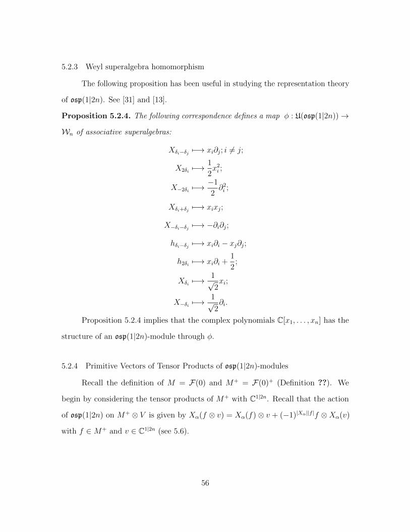
5.2.3 Weyl superalgebra homomorphism

The following proposition has been useful in studying the representation theory

of osp(1|2n). See [31] and [13].

Proposition 5.2.4. The following correspondence defines a map φ : U(osp(1|2n))→

Wn of associative superalgebras:

Xδi−δj 7−→ xi∂j; i 6= j;

X2δi 7−→1

2x2i ;

X−2δi 7−→−1

2∂2i ;

Xδi+δj 7−→ xixj;

X−δi−δj 7−→ −∂i∂j;

hδi−δj 7−→ xi∂i − xj∂j;

h2δi 7−→ xi∂i +1

2;

Xδi 7−→1√2xi;

X−δi 7−→1√2∂i.

Proposition 5.2.4 implies that the complex polynomials C[x1, . . . , xn] has the

structure of an osp(1|2n)-module through φ.

5.2.4 Primitive Vectors of Tensor Products of osp(1|2n)-modules

Recall the definition of M = F(0) and M+ = F(0)+ (Definition ??). We

begin by considering the tensor products of M+ with C1|2n. Recall that the action

of osp(1|2n) on M+ ⊗ V is given by Xα(f ⊗ v) = Xα(f)⊗ v + (−1)|Xα||f |f ⊗Xα(v)

with f ∈M+ and v ∈ C1|2n (see 5.6).

56

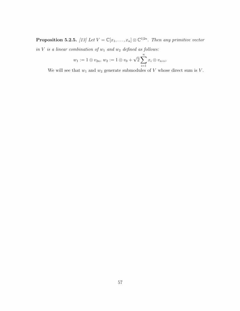
Proposition 5.2.5. [13] Let V = C[x1, . . . , xn]⊗ C1|2n. Then any primitive vector

in V is a linear combination of w1 and w2 defined as follows:

w1 := 1⊗ v2n, w2 := 1⊗ v0 +√

2n∑i=1

xi ⊗ vn+i.

We will see that w1 and w2 generate submodules of V whose direct sum is V .

57

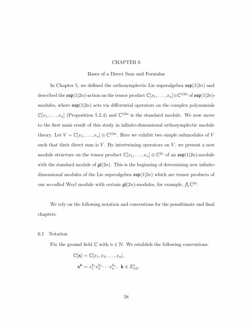
CHAPTER 6

Bases of a Direct Sum and Formulas

In Chapter 5, we defined the orthosymplectic Lie superalgebra osp(1|2n) and

described the osp(1|2n)-action on the tensor product C[x1, . . . , xn]⊗C1|2n of osp(1|2n)-

modules, where osp(1|2n) acts via differential operators on the complex polynomials

C[x1, . . . , xn] (Proposition 5.2.4) and C1|2n is the standard module. We now move

to the first main result of this study in infinite-dimensional orthosymplectic module

theory. Let V = C[x1, . . . , xn]⊗ C1|2n. Here we exhibit two simple submodules of V

such that their direct sum is V . By intertwining operators on V , we present a new

module structure on the tensor product C[x1, . . . , xn]⊗ C2n of an osp(1|2n)-module

with the standard module of gl(2n). This is the beginning of determining new infinite-

dimensional modules of the Lie superalgebra osp(1|2n) which are tensor products of

our so-called Weyl module with certain gl(2n)-modules, for example,∧C2n.

We rely on the following notation and conventions for the penultimate and final

chapters.

6.1 Notation

Fix the ground field C with n ∈ N. We establish the following conventions:

C[x] = C[x1, x2, . . . , xn],

xk = xk11 x

k22 · · ·xknn , k ∈ Zn≥0,

58

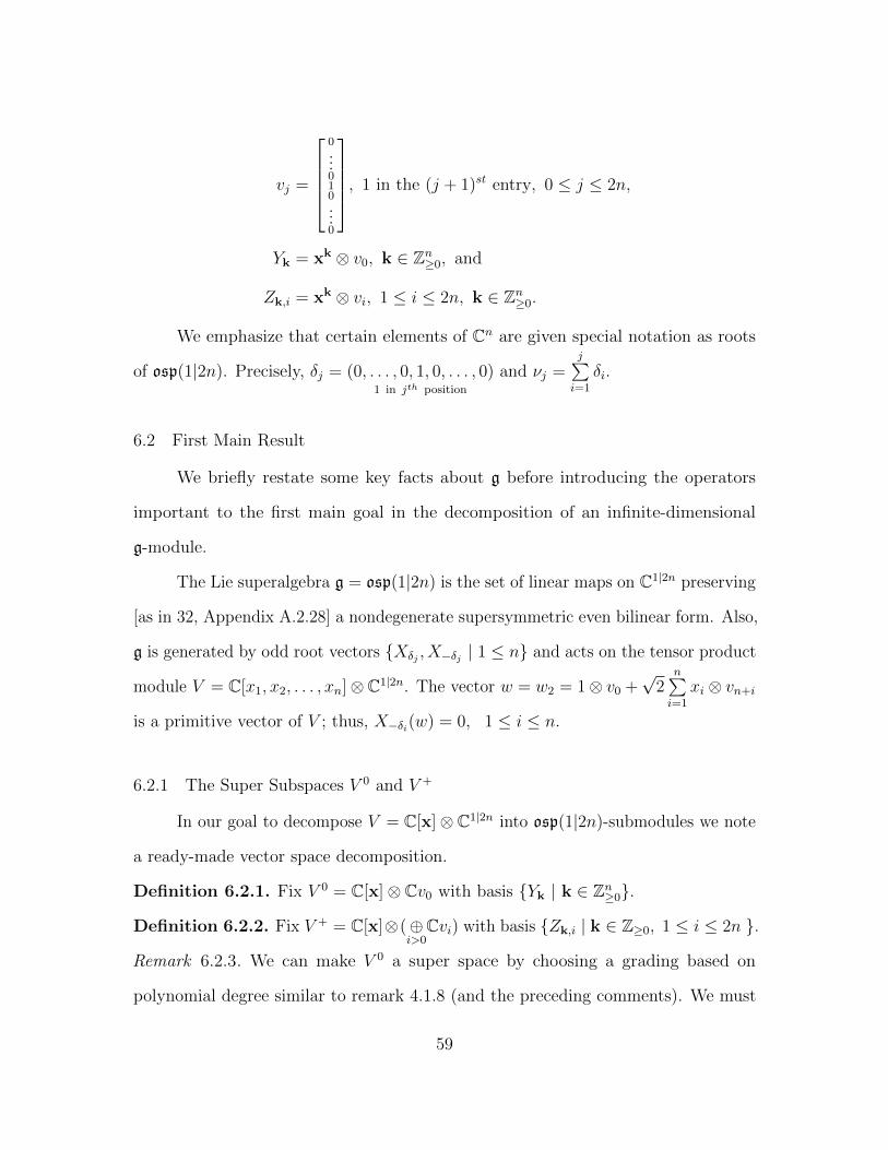
vj =

0...010...0

, 1 in the (j + 1)st entry, 0 ≤ j ≤ 2n,

Yk = xk ⊗ v0, k ∈ Zn≥0, and

Zk,i = xk ⊗ vi, 1 ≤ i ≤ 2n, k ∈ Zn≥0.

We emphasize that certain elements of Cn are given special notation as roots

of osp(1|2n). Precisely, δj = (0, . . . , 0, 1, 0, . . . , 0)1 in jth position

and νj =j∑i=1

δi.

6.2 First Main Result

We briefly restate some key facts about g before introducing the operators

important to the first main goal in the decomposition of an infinite-dimensional

g-module.

The Lie superalgebra g = osp(1|2n) is the set of linear maps on C1|2n preserving

[as in 32, Appendix A.2.28] a nondegenerate supersymmetric even bilinear form. Also,

g is generated by odd root vectors Xδj , X−δj | 1 ≤ n and acts on the tensor product

module V = C[x1, x2, . . . , xn]⊗C1|2n. The vector w = w2 = 1⊗ v0 +√

2n∑i=1

xi ⊗ vn+i

is a primitive vector of V ; thus, X−δi(w) = 0, 1 ≤ i ≤ n.

6.2.1 The Super Subspaces V 0 and V +

In our goal to decompose V = C[x]⊗ C1|2n into osp(1|2n)-submodules we note

a ready-made vector space decomposition.

Definition 6.2.1. Fix V 0 = C[x]⊗ Cv0 with basis Yk | k ∈ Zn≥0.

Definition 6.2.2. Fix V + = C[x]⊗(⊕i>0Cvi) with basis Zk,i | k ∈ Z≥0, 1 ≤ i ≤ 2n .

Remark 6.2.3. We can make V 0 a super space by choosing a grading based on

polynomial degree similar to remark 4.1.8 (and the preceding comments). We must

59

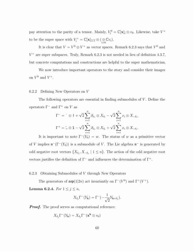
pay attention to the parity of a tensor. Mainly, V 0i = C[x]i ⊗ v0. Likewise, take V +

to be the super space with V +i

= C[x]i+1 ⊗ (⊕i>0Cvi).

It is clear that V = V 0 ⊕ V + as vector spaces. Remark 6.2.3 says that V 0 and

V + are super subspaces. Truly, Remark 6.2.3 is not needed in lieu of definition 4.3.7,

but concrete computations and constructions are helpful to the super mathematician.

We now introduce important operators to the story and consider their images

on V 0 and V +.

6.2.2 Defining New Operators on V

The following operators are essential in finding submodules of V . Define the

operators Γ− and Γ+ on V as

Γ− = 1⊗ 1 +√

2n∑i=1

∂xi ⊗Xδi −√

2n∑i=1

xi ⊗X−δi ,

Γ+ = 1⊗ 1−√

2n∑i=1

∂xi ⊗Xδi +√

2n∑i=1

xi ⊗X−δi .

It is important to note Γ−(Y0) = w. The status of w as a primitive vector

of V implies n−(Γ−(Y0)) is a submodule of V . The Lie algebra n− is generated by

odd negative root vectors Xδj , X−δj | 1 ≤ n. The action of the odd negative root

vectors justifies the definition of Γ− and influences the determination of Γ+.

6.2.3 Obtaining Submodules of V through New Operators

The generators of osp(1|2n) act invariantly on Γ−(V 0) and Γ+(V +).

Lemma 6.2.4. For 1 ≤ j ≤ n,

XδjΓ−(Yk) = Γ−(− 1√

2Yk+δj).

Proof. The proof serves as computational reference:

XδjΓ−(Yk) = XδjΓ

−(xk ⊗ v0)

60

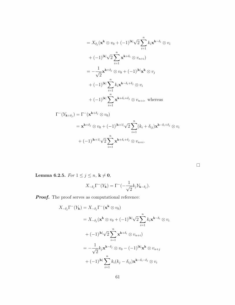
= Xδj(xk ⊗ v0 + (−1)|k|

√2

n∑i=1

kixk−δi ⊗ vi

+ (−1)|k|√

2n∑i=1

xk+δi ⊗ vn+i)

= − 1√2xk+δj ⊗ v0 + (−1)|k|xk ⊗ vj

+ (−1)|k|n∑i=1

kixk−δi+δj ⊗ vi

+ (−1)|k|n∑i=1

xk+δi+δj ⊗ vn+i, whereas

Γ−(Yk+δj) = Γ−(xk+δj ⊗ v0)

= xk+δj ⊗ v0 + (−1)|k+1|√

2n∑i=1

(ki + δij)xk−δi+δj ⊗ vi

+ (−1)|k+1|√

2n∑i=1

xk+δi+δj ⊗ vn+i.

Lemma 6.2.5. For 1 ≤ j ≤ n, k 6= 0,

X−δjΓ−(Yk) = Γ−(− 1√

2kjYk−δj).

Proof. The proof serves as computational reference:

X−δjΓ−(Yk) = X−δjΓ

−(xk ⊗ v0)

= X−δj(xk ⊗ v0 + (−1)|k|

√2

n∑i=1

kixk−δi ⊗ vi

+ (−1)|k|√

2n∑i=1

xk+δi ⊗ vn+i)

= − 1√2kjx

k−δj ⊗ v0 − (−1)|k|xk ⊗ vn+j

+ (−1)|k|n∑i=1

ki(kj − δij)xk−δi−δj ⊗ vi

61

+ (−1)|k|n∑i=1

(kj + δij)xk+δi−δj ⊗ vn+i, whereas

Γ−(Yk−δj) = Γ−(xk−δj ⊗ v0)

= xk−δj ⊗ v0 + (−1)|k−1|√

2n∑i=1

(ki − δij)xk−δi+δj ⊗ vi

+ (−1)|k−1|√

2n∑i=1

xk+δi−δj ⊗ vn+i.

Lemma 6.2.6. For 1 ≤ j ≤ n,

XδjΓ+(Zk,i) = Γ+(

1√2Zk+δj ,i −

√2Zk+δi,j)

and

XδjΓ+(Zk,n+i) = Γ+(

1√2Zk+δj ,n+i +

√2kiZk−δi,j)

Proof. The proof serves as computational reference:

XδjΓ+(Zk,i) = XδjΓ

+(xk ⊗ vi)

= Xδj(xk ⊗ vi + (−1)|k|

√2xk+δi ⊗ v0)

=1√2xk+δj ⊗ vi + (−1)|k|xk+δi+δj ⊗ v0 −

√2xk+δi ⊗ vj and

XδjΓ+(Zk,n+i) = XδjΓ

+(xk ⊗ vn+i)

= Xδj(xk ⊗ vn+i − (−1)|k|

√2kix

k−δi ⊗ v0)

=1√2xk+δj ⊗ vn+i + δij(−1)|k|xk ⊗ v0

− (−1)|k|kixk−δi+δj ⊗ v0 +

√2kix

k−δi ⊗ vj, whereas

Γ+(Zk+δj ,i − Zk+δi,j) = xk+δj ⊗ vi − (−1)|k|√

2xk+δi+δj ⊗ v0

62

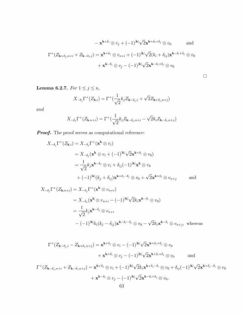
− xk+δi ⊗ vj + (−1)|k|√

2xk+δi+δj ⊗ v0 and

Γ+(Zk+δj ,n+i + Zk−δi,j) = xk+δj ⊗ vn+i + (−1)|k|√

2(ki + δij)xk−δi+δj ⊗ v0

+ xk−δi ⊗ vj − (−1)|k|√

2xk−δi+δj ⊗ v0

Lemma 6.2.7. For 1 ≤ j ≤ n,

X−δjΓ+(Zk,i) = Γ+(

1√2kjZk−δj ,i +

√2Zk+δi,n+j)

and

X−δjΓ+(Zk,n+i) = Γ+(

1√2kjZk−δj ,n+i −

√2kiZk−δi,n+j)

Proof. The proof serves as computational reference:

X−δjΓ+(Zk,i) = X−δjΓ

+(xk ⊗ vi)

= X−δj(xk ⊗ vi + (−1)|k|

√2xk+δi ⊗ v0)

=1√2kjx

k−δj ⊗ vi + δij(−1)|k|xk ⊗ v0

+ (−1)|k|(kj + δij)xk+δi−δj ⊗ v0 +

√2xk+δi ⊗ vn+j and

X−δjΓ+(Zk,n+i) = X−δjΓ

+(xk ⊗ vn+i)

= X−δj(xk ⊗ vn+i − (−1)|k|

√2kix

k−δi ⊗ v0)

=1√2kjx

k−δj ⊗ vn+i

− (−1)|k|ki(kj − δij)xk−δi−δj ⊗ v0 −√

2kixk−δi ⊗ vn+j, whereas

Γ+(Zk−δj ,i − Zk+δi,n+j) = xk+δj ⊗ vi − (−1)|k|√

2xk+δi+δj ⊗ v0

+ xk+δi ⊗ vj − (−1)|k|√

2xk+δi+δj ⊗ v0 and

Γ+(Zk−δj ,n+i + Zk−δi,n+j) = xk+δj ⊗ vi + (−1)|k|√

2kixk+δj−δi ⊗ v0 + δij(−1)|k|

√2xk+δj−δi ⊗ v0

+ xk−δi ⊗ vj − (−1)|k|√

2xk−δi+δj ⊗ v0.

63

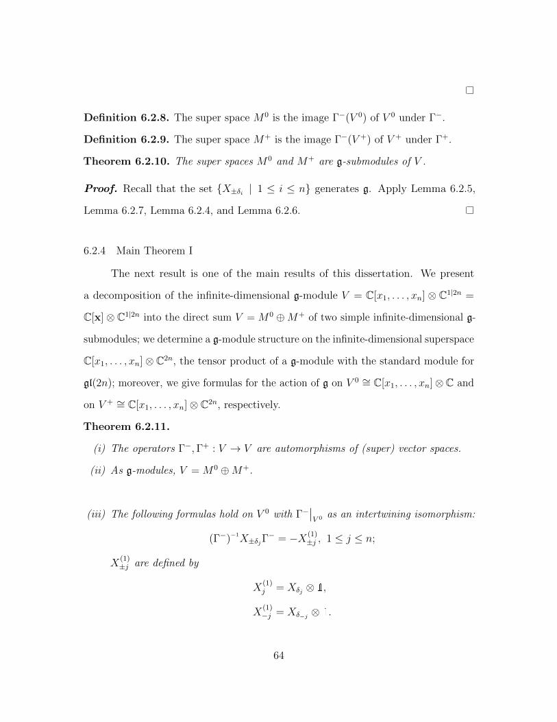
Definition 6.2.8. The super space M0 is the image Γ−(V 0) of V 0 under Γ−.

Definition 6.2.9. The super space M+ is the image Γ−(V +) of V + under Γ+.

Theorem 6.2.10. The super spaces M0 and M+ are g-submodules of V .

Proof. Recall that the set X±δi | 1 ≤ i ≤ n generates g. Apply Lemma 6.2.5,

Lemma 6.2.7, Lemma 6.2.4, and Lemma 6.2.6.

6.2.4 Main Theorem I

The next result is one of the main results of this dissertation. We present

a decomposition of the infinite-dimensional g-module V = C[x1, . . . , xn] ⊗ C1|2n =

C[x]⊗ C1|2n into the direct sum V = M0 ⊕M+ of two simple infinite-dimensional g-

submodules; we determine a g-module structure on the infinite-dimensional superspace

C[x1, . . . , xn]⊗ C2n, the tensor product of a g-module with the standard module for

gl(2n); moreover, we give formulas for the action of g on V 0 ∼= C[x1, . . . , xn]⊗C and

on V + ∼= C[x1, . . . , xn]⊗ C2n, respectively.

Theorem 6.2.11.

(i) The operators Γ−,Γ+ : V → V are automorphisms of (super) vector spaces.

(ii) As g-modules, V = M0 ⊕M+.

(iii) The following formulas hold on V 0 with Γ−∣∣V 0 as an intertwining isomorphism:

(Γ−)−1X±δjΓ− = −X(1)

±j , 1 ≤ j ≤ n;

X(1)±j are defined by

X(1)j = Xδj ⊗ 1,

X(1)−j = Xδ−j ⊗ 1.

64

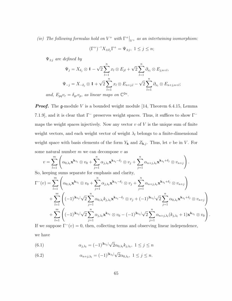
(iv) The following formulas hold on V + with Γ+∣∣V + as an intertwining isomorphism:

(Γ+)−1X±δjΓ+ = Ψ±j, 1 ≤ j ≤ n;

Ψ±j are defined by

Ψj = Xδj ⊗ 1−√

2n∑l=1

xl ⊗ Ejl +√

2n∑l=1

∂xl ⊗ Ej,n+l,

Ψ−j = X−δj ⊗ 1 +√

2n∑l=1

xl ⊗ En+j,l −√

2n∑l=1

∂xl ⊗ En+j,n+l;

and, Epqvr = δqrvp, as linear maps on C2n.

Proof. The g-module V is a bounded weight module [14, Theorem 6.4.15, Lemma

7.1.9], and it is clear that Γ− preserves weight spaces. Thus, it suffices to show Γ−

maps the weight spaces injectively. Now any vector v of V is the unique sum of finite

weight vectors, and each weight vector of weight λl belongs to a finite-dimensional

weight space with basis elements of the form Yk and Zk,j. Thus, let v be in V . For

some natural number m we can decompose v as

v =m∑l=1

(α0,λlx

kλl ⊗ v0 +n∑j=1

αj,λlxkλl−δj ⊗ vj +

n∑j=1

αn+j,λlxkλl+δj ⊗ vn+j

).

So, keeping sums separate for emphasis and clarity,

Γ−(v) =m∑l=1

(α0,λlx

kλl ⊗ v0 +n∑j=1

αj,λlxkλl−δj ⊗ vj +

n∑j=1

αn+j,λlxkλl+δj ⊗ vn+j

)

+m∑l=1

((−1)|kλl |

√2

n∑j=1

α0,λlkj,λlxkλl−δj ⊗ vj + (−1)|kλl |

√2

n∑j=1

α0,λlxkλl+δj ⊗ vn+j

)

+m∑l=1

((−1)|kλl |

√2

n∑j=1

αj,λlxkλl ⊗ v0 − (−1)|kλl |

√2

n∑j=1

αn+j,λl(kj,λl + 1)xkλl ⊗ v0

).

If we suppose Γ−(v) = 0, then, collecting terms and observing linear independence,

we have

αj,λl = (−1)|kλl |√

2α0,λlkj,λl , 1 ≤ j ≤ n(6.1)

αn+j,λl = (−1)|kλl |√

2α0,λl , 1 ≤ j ≤ n.(6.2)

65

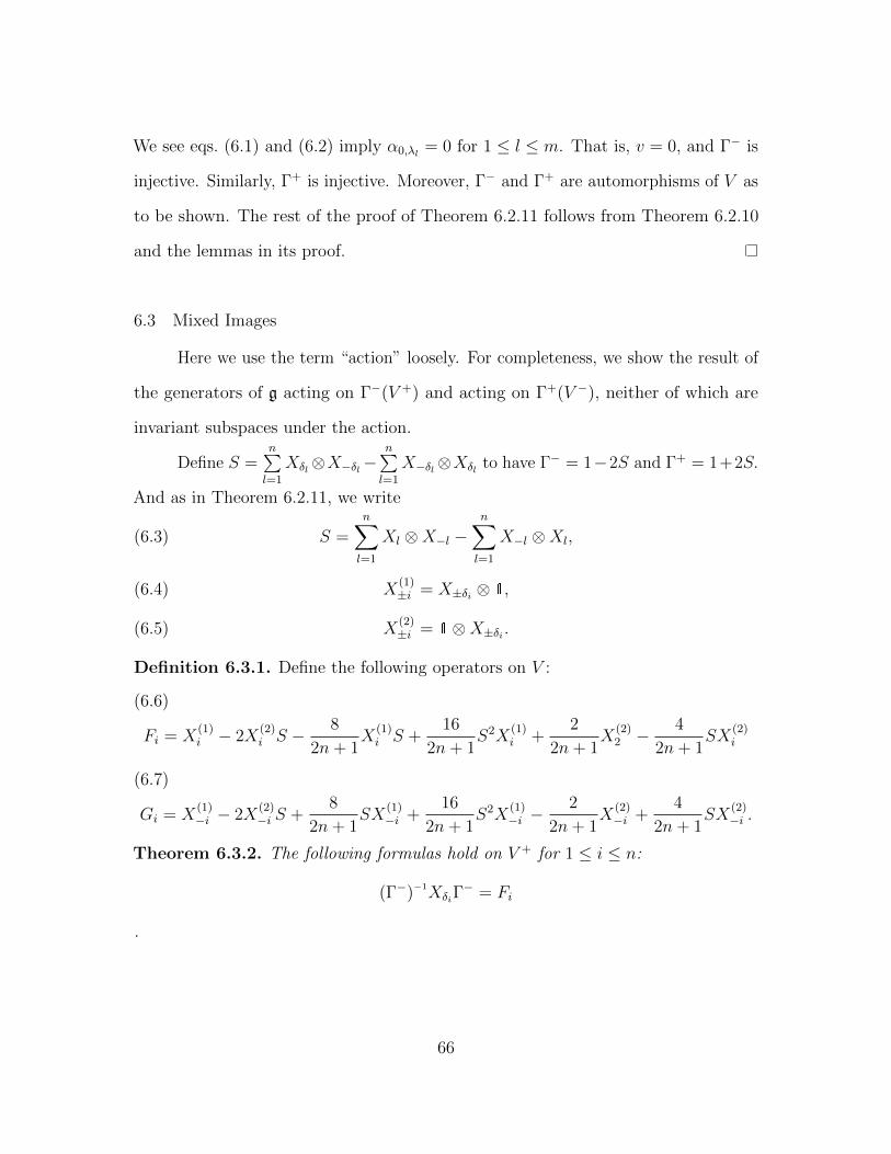
We see eqs. (6.1) and (6.2) imply α0,λl = 0 for 1 ≤ l ≤ m. That is, v = 0, and Γ− is

injective. Similarly, Γ+ is injective. Moreover, Γ− and Γ+ are automorphisms of V as

to be shown. The rest of the proof of Theorem 6.2.11 follows from Theorem 6.2.10

and the lemmas in its proof.

6.3 Mixed Images

Here we use the term “action” loosely. For completeness, we show the result of

the generators of g acting on Γ−(V +) and acting on Γ+(V −), neither of which are

invariant subspaces under the action.

Define S =n∑l=1

Xδl⊗X−δl−n∑l=1

X−δl⊗Xδl to have Γ− = 1−2S and Γ+ = 1+2S.

And as in Theorem 6.2.11, we write

S =n∑l=1

Xl ⊗X−l −n∑l=1

X−l ⊗Xl,(6.3)

X(1)±i = X±δi ⊗ 1,(6.4)

X(2)±i = 1⊗X±δi .(6.5)

Definition 6.3.1. Define the following operators on V :

Fi = X(1)i − 2X

(2)i S − 8

2n+ 1X

(1)i S +

16

2n+ 1S2X

(1)i +

2

2n+ 1X

(2)2 −

4

2n+ 1SX

(2)i

(6.6)

Gi = X(1)−i − 2X

(2)−i S +

8

2n+ 1SX

(1)−i +

16

2n+ 1S2X

(1)−i −

2

2n+ 1X

(2)−i +

4

2n+ 1SX

(2)−i .

(6.7)

Theorem 6.3.2. The following formulas hold on V + for 1 ≤ i ≤ n:

(Γ−)−1XδiΓ− = Fi

.

66

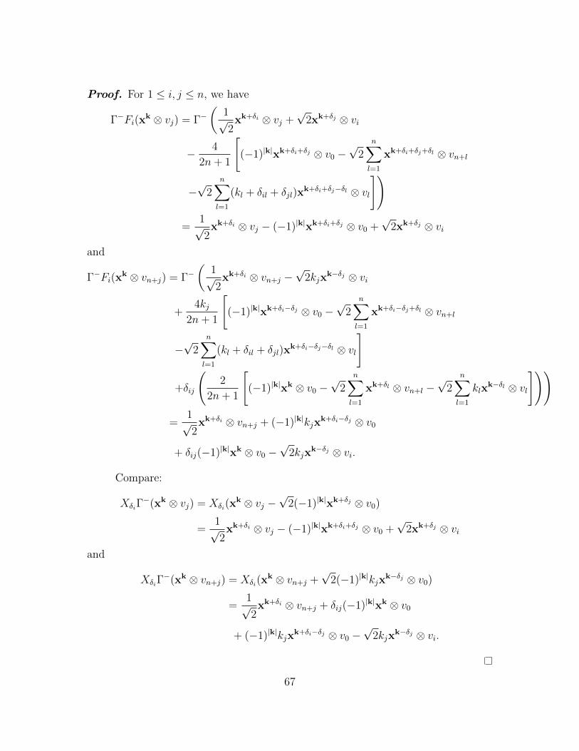
Proof. For 1 ≤ i, j ≤ n, we have

Γ−Fi(xk ⊗ vj) = Γ−

(1√2xk+δi ⊗ vj +

√2xk+δj ⊗ vi

− 4

2n+ 1

[(−1)|k|xk+δi+δj ⊗ v0 −

√2

n∑l=1

xk+δi+δj+δl ⊗ vn+l

−√

2n∑l=1

(kl + δil + δjl)xk+δi+δj−δl ⊗ vl

])

=1√2xk+δi ⊗ vj − (−1)|k|xk+δi+δj ⊗ v0 +

√2xk+δj ⊗ vi

and

Γ−Fi(xk ⊗ vn+j) = Γ−

(1√2xk+δi ⊗ vn+j −

√2kjx

k−δj ⊗ vi

+4kj

2n+ 1

[(−1)|k|xk+δi−δj ⊗ v0 −

√2

n∑l=1

xk+δi−δj+δl ⊗ vn+l

−√

2n∑l=1

(kl + δil + δjl)xk+δi−δj−δl ⊗ vl

]

+δij

(2

2n+ 1

[(−1)|k|xk ⊗ v0 −

√2

n∑l=1

xk+δl ⊗ vn+l −√

2n∑l=1

klxk−δl ⊗ vl

]))

=1√2xk+δi ⊗ vn+j + (−1)|k|kjx

k+δi−δj ⊗ v0

+ δij(−1)|k|xk ⊗ v0 −√

2kjxk−δj ⊗ vi.

Compare:

XδiΓ−(xk ⊗ vj) = Xδi(x

k ⊗ vj −√

2(−1)|k|xk+δj ⊗ v0)

=1√2xk+δi ⊗ vj − (−1)|k|xk+δi+δj ⊗ v0 +

√2xk+δj ⊗ vi

and

XδiΓ−(xk ⊗ vn+j) = Xδi(x

k ⊗ vn+j +√

2(−1)|k|kjxk−δj ⊗ v0)

=1√2xk+δi ⊗ vn+j + δij(−1)|k|xk ⊗ v0

+ (−1)|k|kjxk+δi−δj ⊗ v0 −

√2kjx

k−δj ⊗ vi.

67

Theorem 6.3.3. The following formulas hold on V + for 1 ≤ i ≤ n :

(Γ−)−1X−δiΓ− = Gi

.

Proof. The proof is computationally similar to that of Theorem 6.3.2.

68

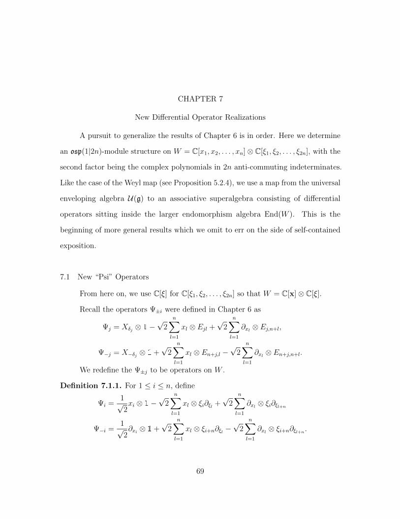
CHAPTER 7

New Differential Operator Realizations

A pursuit to generalize the results of Chapter 6 is in order. Here we determine

an osp(1|2n)-module structure on W = C[x1, x2, . . . , xn]⊗ C[ξ1, ξ2, . . . , ξ2n], with the

second factor being the complex polynomials in 2n anti-commuting indeterminates.

Like the case of the Weyl map (see Proposition 5.2.4), we use a map from the universal

enveloping algebra U(g) to an associative superalgebra consisting of differential

operators sitting inside the larger endomorphism algebra End(W ). This is the

beginning of more general results which we omit to err on the side of self-contained

exposition.

7.1 New “Psi” Operators

From here on, we use C[ξ] for C[ξ1, ξ2, . . . , ξ2n] so that W = C[x]⊗ C[ξ].

Recall the operators Ψ±i were defined in Chapter 6 as

Ψj = Xδj ⊗ 1−√

2n∑l=1

xl ⊗ Ejl +√

2n∑l=1

∂xl ⊗ Ej,n+l,

Ψ−j = X−δj ⊗ 1 +√

2n∑l=1

xl ⊗ En+j,l −√

2n∑l=1

∂xl ⊗ En+j,n+l.

We redefine the Ψ±j to be operators on W .

Definition 7.1.1. For 1 ≤ i ≤ n, define

Ψi =1√2xi ⊗ 1−

√2

n∑l=1

xl ⊗ ξi∂ξl +√

2n∑l=1

∂xl ⊗ ξi∂ξl+n

Ψ−i =1√2∂xi ⊗ 1 +

√2

n∑l=1

xl ⊗ ξi+n∂ξl −√

2n∑l=1

∂xl ⊗ ξi+n∂ξl+n .

69

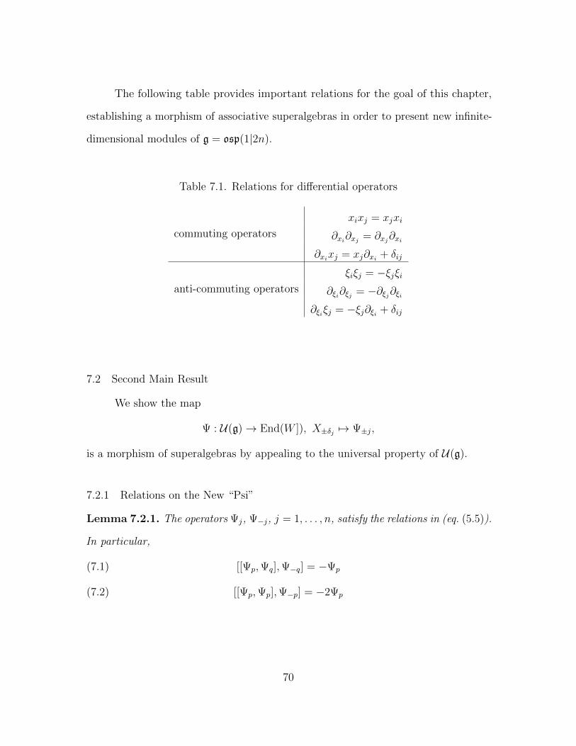
The following table provides important relations for the goal of this chapter,

establishing a morphism of associative superalgebras in order to present new infinite-

dimensional modules of g = osp(1|2n).

Table 7.1. Relations for differential operators

commuting operators

xixj = xjxi

∂xi∂xj = ∂xj∂xi

∂xixj = xj∂xi + δij

anti-commuting operators

ξiξj = −ξjξi∂ξi∂ξj = −∂ξj∂ξi

∂ξiξj = −ξj∂ξi + δij

7.2 Second Main Result

We show the map

Ψ : U(g)→ End(W ]), X±δj 7→ Ψ±j,

is a morphism of superalgebras by appealing to the universal property of U(g).

7.2.1 Relations on the New “Psi”

Lemma 7.2.1. The operators Ψj, Ψ−j, j = 1, . . . , n, satisfy the relations in (eq. (5.5)).

In particular,

[[Ψp,Ψq],Ψ−q] = −Ψp(7.1)

[[Ψp,Ψp],Ψ−p] = −2Ψp(7.2)

70

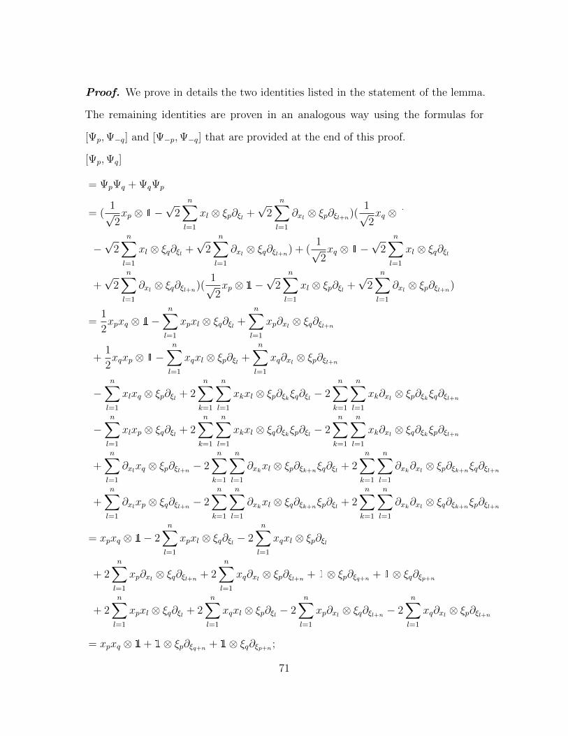
Proof. We prove in details the two identities listed in the statement of the lemma.

The remaining identities are proven in an analogous way using the formulas for

[Ψp,Ψ−q] and [Ψ−p,Ψ−q] that are provided at the end of this proof.

[Ψp,Ψq]

= ΨpΨq + ΨqΨp

= (1√2xp ⊗ 1−

√2

n∑l=1

xl ⊗ ξp∂ξl +√

2n∑l=1

∂xl ⊗ ξp∂ξl+n)(1√2xq ⊗ 1

−√

2n∑l=1

xl ⊗ ξq∂ξl +√

2n∑l=1

∂xl ⊗ ξq∂ξl+n) + (1√2xq ⊗ 1−

√2

n∑l=1

xl ⊗ ξq∂ξl

+√

2n∑l=1

∂xl ⊗ ξq∂ξl+n)(1√2xp ⊗ 1−

√2

n∑l=1

xl ⊗ ξp∂ξl +√

2n∑l=1

∂xl ⊗ ξp∂ξl+n)

=1

2xpxq ⊗ 1−

n∑l=1

xpxl ⊗ ξq∂ξl +n∑l=1

xp∂xl ⊗ ξq∂ξl+n

+1

2xqxp ⊗ 1−

n∑l=1

xqxl ⊗ ξp∂ξl +n∑l=1

xq∂xl ⊗ ξp∂ξl+n

−n∑l=1

xlxq ⊗ ξp∂ξl + 2n∑k=1

n∑l=1

xkxl ⊗ ξp∂ξkξq∂ξl − 2n∑k=1

n∑l=1

xk∂xl ⊗ ξp∂ξkξq∂ξl+n

−n∑l=1

xlxp ⊗ ξq∂ξl + 2n∑k=1

n∑l=1

xkxl ⊗ ξq∂ξkξp∂ξl − 2n∑k=1

n∑l=1

xk∂xl ⊗ ξq∂ξkξp∂ξl+n

+n∑l=1

∂xlxq ⊗ ξp∂ξl+n − 2n∑k=1

n∑l=1

∂xkxl ⊗ ξp∂ξk+nξq∂ξl + 2

n∑k=1

n∑l=1

∂xk∂xl ⊗ ξp∂ξk+nξq∂ξl+n

+n∑l=1

∂xlxp ⊗ ξq∂ξl+n − 2n∑k=1

n∑l=1

∂xkxl ⊗ ξq∂ξk+nξp∂ξl + 2

n∑k=1

n∑l=1

∂xk∂xl ⊗ ξq∂ξk+nξp∂ξl+n

= xpxq ⊗ 1− 2n∑l=1

xpxl ⊗ ξq∂ξl − 2n∑l=1

xqxl ⊗ ξp∂ξl

+ 2n∑l=1

xp∂xl ⊗ ξq∂ξl+n + 2n∑l=1

xq∂xl ⊗ ξp∂ξl+n + 1⊗ ξp∂ξq+n + 1⊗ ξq∂ξp+n

+ 2n∑l=1

xpxl ⊗ ξq∂ξl + 2n∑l=1

xqxl ⊗ ξp∂ξl − 2n∑l=1

xp∂xl ⊗ ξq∂ξl+n − 2n∑l=1

xq∂xl ⊗ ξp∂ξl+n

= xpxq ⊗ 1 + 1⊗ ξp∂ξq+n + 1⊗ ξq∂ξp+n ;

71

[[Ψp,Ψq],Ψ−q]

= (xpxq ⊗ 1 + 1⊗ ξp∂ξq+n + 1⊗ ξq∂ξp+n)(1√2∂xq ⊗ 1 +

√2

n∑l=1

xl ⊗ ξq+n∂ξl

−√

2n∑l=1

∂xl ⊗ ξq+n∂ξl+n)− (1√2∂xq ⊗ 1 +

√2

n∑l=1

xl ⊗ ξq+n∂ξl

−√

2n∑l=1

∂xl ⊗ ξq+n∂ξl+n)(xpxq ⊗ 1 + 1⊗ ξp∂ξq+n + 1⊗ ξq∂ξp+n)

=1√2xpxq∂xq ⊗ 1 +

√2

n∑l=1

xpxqxl ⊗ ξq+n∂ξl −√

2n∑l=1

xpxq∂xl ⊗ ξq+n∂ξl+n

+1√2∂xq ⊗ ξp∂ξq+n +

√2

n∑l=1

xl ⊗ ξp∂ξq+nξq+n∂ξl −√

2n∑l=1

∂xl ⊗ ξp∂ξq+nξq+n∂ξl+n

+1√2∂xq ⊗ ξq∂ξp+n +

√2

n∑l=1

xl ⊗ ξq∂ξp+nξq+n∂ξl −√

2n∑l=1

∂xl ⊗ ξq∂ξp+nξq+n∂ξl+n

− 1√2∂xqxpxq ⊗ 1− 1√

2∂xq ⊗ ξp∂ξq+n −

1√2∂xq ⊗ ξq∂ξp+n

−√

2n∑l=1

xlxpxq ⊗ ξq+n∂ξl −√

2n∑l=1

xl ⊗ ξq+n∂ξlξp∂ξq+n −√

2n∑l=1

xl ⊗ ξq+n∂ξlξq∂ξp+n

+√

2n∑l=1

∂xlxpxq ⊗ ξq+n∂ξl+n +√

2n∑l=1

∂xl ⊗ ξq+n∂ξl+nξp∂ξq+n +√

2n∑l=1

∂xl ⊗ ξq+n∂ξl+nξq∂ξp+n

= − 1√2xp ⊗ 1 +

√2xp ⊗ ξq+n∂ξq+n +

√2xq ⊗ ξq+n∂ξp+n

−√

2xp ⊗ ξq+n∂ξq+n +√

2n∑l=1

xl ⊗ ξp∂ξl −√

2n∑l=1

∂xl ⊗ ξp∂ξl+n

−√

2xq ⊗ ξq+n∂ξp+n

= −Ψp,

72

[Ψp,Ψp]

= 2ΨpΨp

= 2(1√2xp ⊗ 1−

√2

n∑l=1

xl ⊗ ξp∂ξl +√

2n∑l=1

∂xl ⊗ ξp∂ξl+n)(1√2xp ⊗ 1

−√

2n∑l=1

xl ⊗ ξp∂ξl +√

2n∑l=1

∂xl ⊗ ξp∂ξl+n)

= x2p ⊗ 1− 2

n∑l=1

xpxl ⊗ ξp∂ξl + 2n∑l=1

xp∂xl ⊗ ξp∂ξl+n

− 2n∑l=1

xlxp ⊗ ξp∂ξl + 4n∑k=1

n∑l=1

xkxl ⊗ ξp∂ξkξp∂ξl − 4n∑k=1

n∑l=1

xk∂xl ⊗ ξp∂ξkξp∂ξl+n

+ 2n∑l=1

∂xlxp ⊗ ξp∂ξl+n − 4n∑k=1

n∑l=1

∂xkxl ⊗ ξp∂ξk+nξp∂ξl + 4

n∑k=1

n∑l=1

∂xk∂xl ⊗ ξp∂ξk+nξp∂ξl+n)

= x2p ⊗ 1− 4

n∑l=1

xpxl ⊗ ξp∂ξl + 4n∑l=1

xp∂xl ⊗ ξp∂ξl+n + 2⊗ ξp∂ξp+n

+ 4n∑l=1

xpxl ⊗ ξp∂ξl − 2n∑l=1

xp∂xl ⊗ ξp∂ξl+n

= x2p ⊗ 1 + 2⊗ ξp∂ξp+n ;

73

[[Ψp,Ψp],Ψ−p]

= (x2p ⊗ 1 + 2⊗ ξp∂ξp+n)(

1√2∂xp ⊗ 1 +

√2

n∑l=1

xl ⊗ ξp+n∂ξl −√

2n∑l=1

∂xl ⊗ ξp+n∂ξl+n)

− (1√2∂xp ⊗ 1 +

√2

n∑l=1

xl ⊗ ξp+n∂ξl −√

2n∑l=1

∂xl ⊗ ξp+n∂ξl+n)(x2p ⊗ 1 + 2⊗ ξp∂ξp+n)

=1√2x2p∂xp ⊗ 1 +

√2

n∑l=1

x2pxl ⊗ ξp+n∂ξl −

√2

n∑l=1

x2p∂xl ⊗ ξp+n∂ξl+n

+√

2∂xp ⊗ ξp∂ξp+n + 2√

2n∑l=1

xl ⊗ ξp∂ξp+nξp+n∂ξl − 2√

2n∑l=1

∂xl ⊗ ξp∂ξp+nξp+n∂ξl+n

− 1√2∂xpx

2p ⊗ 1−

√2∂xp ⊗ ξp∂ξp+n

−√

2n∑l=1

xlx2p ⊗ ξp+n∂ξl − 2

√2

n∑l=1

xl ⊗ ξp+n∂ξlξp∂ξp+n

+√

2n∑l=1

∂xlx2p ⊗ ξp+n∂ξl+n + 2

√2

n∑l=1

∂xl ⊗ ξp+n∂ξl+nξp∂ξp+n

= −2xp ⊗ 1 + 2√

2xp ⊗ ξp+n∂ξp+n − 2√

2xp ⊗ ξp+n∂ξp+n

+ 2√

2n∑l=1

xp ⊗ ξp∂ξl − 2√

2n∑l=1

∂xp ⊗ ξp∂ξl+n

= −2Ψp.

74

[Ψp,Ψ−q]

= ΨpΨ−q + Ψ−qΨp

= (1√2xp ⊗ 1−

√2

n∑l=1

xl ⊗ ξp∂ξl +√

2n∑l=1

∂xl ⊗ ξp∂ξl+n)(1√2∂xq ⊗ 1

+√

2n∑l=1

xl ⊗ ξq+n∂ξl −√

2n∑l=1

∂xl ⊗ ξq+n∂ξl+n)

+ (1√2∂xq ⊗ 1 +

√2

n∑l=1

xl ⊗ ξq+n∂ξl −√

2n∑l=1

∂xl ⊗ ξq+n∂ξl+n)(1√2xp ⊗ 1

−√

2n∑l=1

xl ⊗ ξp∂ξl +√

2n∑l=1

∂xl ⊗ ξp∂ξl+n)

=1

2xp∂xq ⊗ 1 +

n∑l=1

xpxl ⊗ ξq+n∂ξl −n∑l=1

xp∂xl ⊗ ξq+n∂ξl+n

−n∑l=1

xl∂xq ⊗ ξp∂ξl − 2n∑k=1

n∑l=1

xkxl ⊗ ξp∂ξkξq+n∂ξl + 2n∑k=1

n∑l=1

xk∂xl ⊗ ξp∂ξkξq+n∂ξl+n

+n∑l=1

∂xl∂xq ⊗ ξp∂ξl+n + 2n∑k=1

n∑l=1

∂xkxl ⊗ ξp∂ξk+nξq+n∂ξl − 2

n∑k=1

n∑l=1

∂xk∂xl ⊗ ξp∂ξk+nξq+n∂ξl+n

+1

2∂xqxp ⊗ 1−

n∑l=1

∂xqxl ⊗ ξp∂ξl +n∑l=1

∂xq∂xl ⊗ ξp∂ξl+n

+n∑l=1

xlxp ⊗ ξq+n∂ξl − 2n∑k=1

n∑l=1

xkxl ⊗ ξq+n∂ξkξp∂ξl + 2n∑k=1

n∑l=1

xk∂xl ⊗ ξq+n∂ξkξp∂ξl+n

−n∑l=1

∂xlxp ⊗ ξq+n∂ξl+n + 2n∑k=1

n∑l=1

∂xkxl ⊗ ξq+n∂ξk+nξp∂ξl − 2

n∑k=1

n∑l=1

∂xk∂xl ⊗ ξq+n∂ξk+nξp∂ξl+n

= xp∂xq ⊗ 1 +δpq2⊗ 1 + 2

n∑l=1

xpxl ⊗ ξq+n∂ξl − 2n∑l=1

xp∂xl ⊗ ξq+n∂ξl+n − 1⊗ ξq+n∂ξp+n

− 2n∑l=1

xl∂xq ⊗ ξp∂ξl − 1⊗ ξp∂ξq − 2n∑l=1

xpxl ⊗ ξq+n∂ξl + 2n∑l=1

xp∂xl ⊗ ξq+n∂ξl+n

+ 2n∑l=1

∂xq∂xl ⊗ ξp∂ξl+n + 2n∑l=1

∂xqxl ⊗ ξp∂ξl − 2n∑l=1

∂xq∂xl ⊗ ξp∂ξl+n

= xp∂xq +δpq2⊗ 1 + 1⊗ ξp∂ξq − 1⊗ ξq+n∂ξp+n ;

75

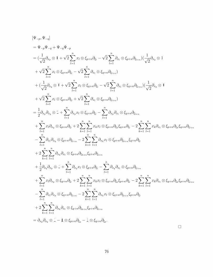
[Ψ−p,Ψ−q]

= Ψ−pΨ−q + Ψ−qΨ−p

= (1√2∂xp ⊗ 1 +

√2

n∑l=1

xl ⊗ ξp+n∂ξl −√

2n∑l=1

∂xl ⊗ ξp+n∂ξl+n)(1√2∂xq ⊗ 1

+√

2n∑l=1

xl ⊗ ξq+n∂ξl −√

2n∑l=1

∂xl ⊗ ξq+n∂ξl+n)

+ (1√2∂xq ⊗ 1 +

√2

n∑l=1

xl ⊗ ξq+n∂ξl −√

2n∑l=1

∂xl ⊗ ξq+n∂ξl+n)(1√2∂xp ⊗ 1

+√

2n∑l=1

xl ⊗ ξp+n∂ξl +√

2n∑l=1

∂xl ⊗ ξp+n∂ξl+n)

=1

2∂xp∂xq ⊗ 1 +

n∑l=1

∂xpxl ⊗ ξq+n∂ξl −n∑l=1

∂xp∂xl ⊗ ξq+n∂ξl+n

+n∑l=1

xl∂xq ⊗ ξp+n∂ξl + 2n∑k=1

n∑l=1

xkxl ⊗ ξp+n∂ξkξq+n∂ξl − 2n∑k=1

n∑l=1

xk∂xl ⊗ ξp+n∂ξkξq+n∂ξl+n

−n∑l=1

∂xl∂xq ⊗ ξp+n∂ξl+n − 2n∑k=1

n∑l=1

∂xkxl ⊗ ξp+n∂ξk+nξq+n∂ξl

+ 2n∑k=1

n∑l=1

∂xk∂xl ⊗ ξp+n∂ξk+nξq+n∂ξl+n

+1

2∂xq∂xp ⊗ 1 +

n∑l=1

∂xqxl ⊗ ξp+n∂ξl −n∑l=1

∂xq∂xl ⊗ ξp+n∂ξl+n

+n∑l=1

xl∂xp ⊗ ξq+n∂ξl + 2n∑k=1

n∑l=1

xkxl ⊗ ξq+n∂ξkξp+n∂ξl − 2n∑k=1

n∑l=1

xk∂xl ⊗ ξq+n∂ξkξp+n∂ξl+n

−n∑l=1

∂xl∂xp ⊗ ξq+n∂ξl+n − 2n∑k=1

n∑l=1

∂xkxl ⊗ ξq+n∂ξk+nξp+n∂ξl

+ 2n∑k=1

n∑l=1

∂xk∂xl ⊗ ξq+n∂ξk+nξp+n∂ξl+n

= ∂xp∂xq ⊗ 1− 1⊗ ξp+n∂ξq − 1⊗ ξq+n∂ξp .

76

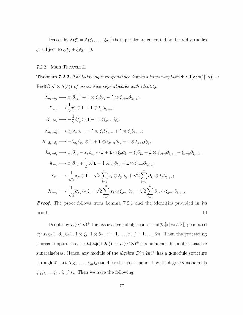
Denote by Λ(ξ) = Λ(ξ1, . . . , ξ2n) the superalgebra generated by the odd variables

ξi subject to ξiξj + ξjξi = 0.

7.2.2 Main Theorem II

Theorem 7.2.2. The following correspondence defines a homomorphism Ψ : U(osp(1|2n))→

End(C[x]⊗ Λ(ξ)) of associative superalgebras with identity:

Xδp−δq 7−→ xp∂xq1 + 1⊗ ξp∂ξq − 1⊗ ξq+n∂ξp+n ;

X2δp 7−→1

2x2p ⊗ 1 + 1⊗ ξp∂ξp+n ;

X−2δp 7−→ −1

2∂2xp ⊗ 1− 1⊗ ξp+n∂ξp ;

Xδp+δq 7−→ xpxq ⊗ 1 + 1⊗ ξp∂ξq+n + 1⊗ ξq∂ξp+n ;

X−δp−δq 7−→ −∂xp∂xq ⊗ 1 + 1⊗ ξp+n∂ξq + 1⊗ ξq+n∂ξp ;

hδp−δq 7−→ xp∂xq − xq∂xp ⊗ 1 + 1⊗ ξp∂ξp − ξq∂ξq + 1⊗ ξq+n∂ξq+n − ξp+n∂ξp+n ;

h2δp 7−→ xp∂xp +1

2⊗ 1 + 1⊗ ξp∂ξp − 1⊗ ξp+n∂ξp+n ;

Xδp 7−→1√2xp ⊗ 1−

√2

n∑l=1

xl ⊗ ξp∂ξl +√

2n∑l=1

∂xl ⊗ ξp∂ξl+n ;

X−δp 7−→1√2∂xp ⊗ 1 +

√2

n∑l=1

xl ⊗ ξp+n∂ξl −√

2n∑l=1

∂xl ⊗ ξp+n∂ξl+n .

Proof. The proof follows from Lemma 7.2.1 and the identities provided in its

proof.

Denote by D(n|2n)+ the associative subalgebra of End(C[x]⊗ Λ[ξ]) generated

by xi ⊗ 1, ∂xi ⊗ 1, 1⊗ ξj, 1⊗ ∂ξj , i = 1, . . . , n, j = 1, . . . , 2n. Then the proceeding

theorem implies that Ψ : U(osp(1|2n))→ D(n|2n)+ is a homomorphism of associative

superalgebras. Hence, any module of the algebra D(n|2n)+ has a g-module structure

through Ψ. Let Λ(ξ1, . . . , ξ2n)d stand for the space spanned by the degree d monomials

ξi1ξi2 . . . ξid , it 6= is. Then we have the following.

77

Corollary 7.2.3. The super spaces C[x]⊗ Λ[ξ] and C[x]⊗ Λ[ξ]d have structures of

osp(1|2n)-modules.

The methods of Chapter 6 are now in play.

7.2.3 New Idea

The preceding results can be re-framed without tensor products and using

non-conventional relations on the even and odd variables.

Remark 7.2.4. We can consider different grading on D(n|2n)+ and define the variable

ξi and their derivatives to be even. In fact, using the ideas of [20], we have a more

invariant description. Namely, if we first fix n odd variables xi and 2n even variables

ξp, satisfying xixj − xjxi = xiξp + ξpxi = ξpξq + ξqξp = 0. Then we introduce

derivations ∂xi and ∂ξj and relations between the derivations that are analogous t

those between the variables. The resulting superalgebra is denoted by A+n|2n and we

obtain a homomorphism U(osp(1|2n))→ A+n|2n.

78

REFERENCES

[1] Axler, S. (2014). Linear algebra done right. New York, Springer.

[2] Bartocci, C., Bruzzo, U., & Hernandez-Ruiperez, D. (1991). The geometry of

supermanifolds. Dordrecht ; Boston, Kluwer Academic Publishers.

[3] Berezin, F. A. (2010). Introduction to superanalysis. Place of publication not

identified, Springer.

[4] Bernstein, J. N., & Gelfan, S. I. (1980). Tensor products of finite and infinite

dimensional representations of semisimple Lie algebras. Compositio Mathematica,

Volume 41 (no. 2), 245–285.

[5] Cheng, S.-J., & Wang, W. (2012). Dualities and representations of Lie super-

algebras (Vol. 144). American Mathematical Society, Providence, RI. https:

//doi.org/10.1090/gsm/144

[6] Coulembier, K. (2010). The orthosymplectic lie supergroup in harmonic analysis,

In AIP Conference Proceedings. https://doi.org/10.1063/1.3498035

[7] Coulembier, K. (2013). On a class of tensor product representations for the

orthosymplectic superalgebra. Journal of Pure and Applied Algebra, 217 (5),

819–837. https://doi.org/10.1016/j.jpaa.2012.09.009

[8] Coulembier, K., Somberg, P., & Soucek, V. (2014). Joseph ideals and harmonic

analysis for osp(m|2n). International Mathematics Research Notices, 2014 (15),

4291–4340. https://doi.org/10.1093/imrn/rnt074

[9] Dimitrov, I., Mathieu, O., & Penkov, I. (2000). On the structure of weight

modules. Transactions of the American Mathematical Society, 352 (6), 2857–

2869. https://doi.org/10.1090/S0002-9947-00-02390-4

79

[10] Erdmann, K., & Wildon, M. J. (2006). Introduction to Lie algebras. London,

Springer.

[11] Farmer, R. (1984). Orthosymplectic superalgebras in mathemathics and physics

(PhD Thesis). Tasmania U.

[12] Fayet, P., & Ferrara, S. (1977). Supersymmetry. Physics Reports. A Review

Section of Physics Letters, 32C (5), 249–334. https://doi.org/10.1016/0370-

1573(77)90066-7

[13] Ferguson, T. (2015). Weight modules of orthosymplectic Lie superalgebras (PhD

Thesis). The University of Texas at Arlington.

[14] Ferguson, T., Gorelik, M., & Grantcharov, D. (2016). Bounded highest weight

modules over osp(1, 2n). In Lie algebras, lie superalgebras, vertex algebras and

related topics (pp. 135–144). Amer. Math. Soc., Providence, RI.

[15] Frappat, L., Sciarrino, A., & Sorba, P. (2000). Dictionary on Lie algebras and

superalgebras. Academic Press, Inc., San Diego, CA.

[16] Ganchev, A. C., & Palev, T. D. (1980). A Lie superalgebraic interpretation

of the para-Bose statistics. Journal of Mathematical Physics, 21 (4), 797–799.

https://doi.org/10.1063/1.524502

[17] Goodman, R., & Wallach, N. R. (2009). Symmetry, representations, and invari-

ants. Dordrecht [Netherlands] ; New York, Springer.

[18] Gorelik, M., & Grantcharov, D. (2018). Simple bounded highest weight modules

of basic classical Lie superalgebras, arxiv 1812.11593v1.

[19] Grantcharov, D., & Williams, I., Dwight. (n.d.). Bases of infinite-dimensional

tensor product representations of osp(1|2n) (Unpublished).

[20] Hartwig, J. T., & Serganova, V. (2018). Clifford and Weyl superalgebras and

spinor representations. arXiv:1807.04220 [math], arxiv 1807.04220.

80

[21] Humphreys, J. E. (1994). Introduction to Lie algebras and representation theory

(6th corr. print). New York, Springer-Verlag.

[22] Hungerford, T. W. (2003). Algebra (Corr. 8th print). New York, Springer.

[23] Kac, V. (1975). Classification of simple Lie superalgebras. Funktsional. Anal. i

Prilozhen, 9 (3), 91–92.

[24] Kac, V. (1977). Lie superalgebras. Advances in mathematics, 26 (1), 8–96.

[25] Kostant, B. (1975). On the tensor product of a finite and an infinite dimensional

representation. Journal of Functional Analysis, 20 (4), 257–285. https://doi.

org/10.1016/0022-1236(75)90035-X

[26] Lang, S. (1993). Real and functional analysis (3rd ed). New York, Springer-

Verlag.

[27] Lang, S. (2005). Structure of bilinear forms. In Algebra. New York, Springer.

[28] Leites, D. A. (1980). Introduction to the theory of supermanifolds. Russian Math-

ematical Surveys, 35 (1), 1–64. https://doi.org/10.1070/RM1980v035n01ABEH001545

[29] Manin, Y. (2018). Quantum groups and non-commutative geometry. New York,

NY, Springer Berlin Heidelberg.

[30] Manin, Y. I. (1997). Introduction to supergeometry. In Y. I. Manin (Ed.),

Gauge Field Theory and Complex Geometry (pp. 181–232). Berlin, Heidelberg,

Springer Berlin Heidelberg. https://doi.org/10.1007/978-3-662-07386-5 5

[31] Musson, I. M. (1999). Lie superalgebras associated to the Weyl algebras. Pro-

ceedings of the American Mathematical Society, Vol. 127 (No. 10), 2821–2827.

[32] Musson, I. M. (2012). Lie superalgebras and enveloping algebras. Providence,

R.I, American Mathematical Society.

[33] Riehl, E. (2016). Category theory in context. Mineola, New York, Dover Publi-

cations.

81

[34] Rossmann, W. (2006). Lie groups: An introduction through linear groups (Pa-

perback). Oxford New York Auckland, Oxford University Press.

[35] Rynne, B. P., & Youngson, M. A. (2008). Linear functional analysis (2nd ed).

London, Springer.

[36] Samelson, H. (1990). Notes on Lie algebras (New, rev. ed.). New York, NY

Berlin, Springer.

[37] Shafarevich, I. R., Kostrikin, A. I., & Reid, M. (2005). Basic notions of algebra

(3. printing). Berlin, Springer.

[38] Shilov, G. E. (1977). Linear algebra (Rev. English ed). New York, Dover

Publications.

[39] Stillwell, J. (2008). Naive lie theory. New York ; London, Springer.

[40] Tuynman, G. M. (2010). Supermanifolds and supergroups: Basic theory. Dor-

drecht, Kluwer Academic Publishers.

[41] Whitehead, J. (1941). On Adding Relations to Homotopy Groups. The Annals

of Mathematics, 42 (2), 409. https://doi.org/10.2307/1968907

[42] Williams, R. E. (1988). Finite dimensional Hopf algebras.

[43] Zuckerman, G. (1977). Tensor products of finite and infinite dimensional repre-

sentations of semisimple Lie groups. The Annals of Mathematics, 106 (2), 295.

https://doi.org/10.2307/1971097

[44] Zumino, B. (2006). Supersymmetry then and now. Fortschritte der Physik.

Progress of Physics, 54 (2-3), 199–204. https://doi.org/10.1002/prop.200510268

82

BIOGRAPHICAL STATEMENT

Dwight Anderson Williams II was born in Saint Paul, MN, in 1989. He

received his B.S. from Florida Agricultural & Mechanical University in 2012 and

M.S degree from Florida State University in 2014, both degrees in mathematics

and both institutions of Tallahassee, Florida. He re-committed to his doctoral

studies by entering the Department of Mathematics at The University of Texas

at Arlington during Fall 2016. His research interests focus on infinite-dimensional

representations of Lie superalgebras along with various justifications for calling himself

a “supermathemathician”. His vision is MathChange: a river of thought leading to

a delta of change through the flow of mathematical discourse as an innate element of

humanity reflected in our shared experiences.

83