www.sciencemag.org/content/352/6285/604/suppl/DC1

Supplementary Materials for Broken detailed balance at mesoscopic scales in active biological

systems

Christopher Battle, Chase P. Broedersz, Nikta Fakhri, Veikko F. Geyer, Jonathon Howard, Christoph F. Schmidt,* Fred C. MacKintosh*

*Corresponding author. Email: fcmack@gmail.com (F.C.M.); christoph.schmidt@phys.uni-goettingen.de(C.F.S.)

Published 29 April 2016, Science 352, 604 (2016) DOI: 10.1126/science.aac8167

This PDF file includes:

Materials and Methods Figs. S1 to S17 Captions for Movies S1 and S2 References (37–54)

Other Supplementary Materials for this manuscript include the following: (available at www.sciencemag.org/content/352/6285/604/suppl/DC1)

Movies S1 and S2

SupplementaryMaterialsfor:

Broken detailed balance at the mesoscale in activebiologicalsystemsAuthors:ChristopherBattle1,7*,ChaseP.Broedersz2,3,7*,NiktaFakhri1,4,7*,VeikkoF.Geyer5,JonathonHoward5,ChristophF.Schmidt1,7,+,andFredC.MacKintosh6,7,+

* Authorscontributedequally+Correspondingauthors

Affiliations:1DrittesPhysikalischesInstitut,Georg-August-Universität,37077Göttingen,Germany2Lewis–SiglerInstituteforIntegrativeGenomicsandJosephHenryLaboratoriesofPhysics,PrincetonUniversity,Princeton,NJ08544,USA3Arnold-Sommerfeld-CenterforTheoreticalPhysicsandCenterforNanoScience,Ludwig-Maximilians-UniversitätMünchen,Theresienstrasse37,D-80333München,Germany4DepartmentofPhysics,MassachusettsInstituteofTechnology,Cambridge,MA02139,USA5DepartmentofMolecularBiophysics&Biochemistry,YaleUniversity,NewHaven,Connecticut,USA6DepartmentofPhysicsandAstronomy,VUUniversity,Amsterdam,TheNetherlands7TheKavliInstituteforTheoreticalPhysics,UniversityofCaliforniaSantaBarbara,CA93106,USA

MaterialsandMethods:

1Probabilityfluxanalysis(PFA)

HerewedescribehowweanalyzeexperimentaltimetracestodetermineprobabilityfluxesinaCoarseGrainedPhaseSpace(CGPS).Ingeneral,therawtimetracesrepresenthighlystochastictrajectories through phase space, in which case broken detailed balance only becomesapparentwhen the statistics of transitions between configurations are analyzed over a longtime window. Thus we infer a non-zero average flux or current in phase space when theprobability for a particular transition in CGPS is unequal to the probability for the reversetransition. The statistical significance of this current is determined through the use of abootstrappingmethoddescribedbelow.

Suchstatisticallynon-reciprocaldynamicsshouldbecontrastedwiththecaseofdeterministicnon-reciprocalmotion.Anexampleforthelatteristheobviouslynon-reciprocaltrajectoriesofactiveflagella(37, 38)(seealsoFigure1),oractiveswimmers(39).

1.1Coarsegrainingprocedure:analyzingcontinuoustimetrajectoriesusingdiscretized low-dimensional projections of phase space: We consider a stationary dynamic system thatneverthelessevolvesintimeonshorttimescalesduetothermalornon-thermalfluctuationsoroscillations. Among the set of coordinates that constitute a full specification of theconfigurationof thesystem,weobserveor track inouranalysis𝐷 coordinates𝑥!,… , 𝑥!.Theremaining 𝑀 coordinates 𝑥!,… , 𝑥! are not tracked. Since these coordinates can take onarbitrary values without our knowledge, they will be integrated out below. We, for themoment,onlyconsiderspatialorconformationaldegreesoffreedombecausemomentuminatypicaloverdampedbiologicalsoft-mattersystemrelaxesontime-scalesthataremuchshorterthanthetemporalresolutionofourexperiments.Forconvenience,wehaveplacedatildeonthedegreesoffreedomthatwillbeintegratedoutbelow.

Ourchoiceofcoordinatestodescribetheconfigurationofthesystemisarbitrary,anddoesnotneed tocorrespond, for instance, to thepositionsofallparticles. Ingeneral,wecanuseanycomplete set of generalized coordinates. These generalized coordinates can be linear ornonlinearfunctionsoftheparticlepositions,viaacoordinatetransformation.Inthemaintextweconsiderthreecases:(1)where𝑥!,… , 𝑥!arenormalmodeamplitudesoftheflagellum,(2)coordinatesofparticlescoupledthroughaspring,and(3)theangleandcurvatureofacilium.Ineachcase,thesecanbeconsideredtobefunctions,e.g.,ofalltheparticlesinthesystem.Sincethesecoarse-grainedcoordinatesare independent, they canalsobeconsidered to constitutepartofafullsetofgeneralizedcoordinates𝑥!,… , 𝑥!,𝑥!,… , 𝑥!describingthephasespaceofthesystem.WenotethatothervariablessuchasparticleconcentrationorpHmayalsobeusedasgeneralizedcoordinatesofthesystem.

Sincethesystemisstationary,wecandefineaprobabilitydensitythatdescribeshowlikelyitisto find the system in a certain configuration. The dynamics of the system then satisfies thecontinuityequation:

∫!𝑑!𝑥𝑑!𝑥 !"(!!,…,!!,!!,…,!!,!)

!"= −∫!Ω𝚥 ⋅ 𝑑𝑠 (S1)

where𝜌istheprobabilitydensityand𝚥isthecurrentdensitydescribingtheaveragemotionofthe system in the configurational phase space. Here, we consider a region of phase spacecorrespondingtosomesubsetΩ!ofthecoordinatesthatwetrack(𝑥!,… , 𝑥!).Sincewedonottrack the remaining coordinates𝑥!,… , 𝑥!,we thus consider a subset in the full phase spacedefinedbyΩ = Ω!×Ω!,whereΩ! represents the space spannedby the coordinates𝑥!,… ,𝑥!.

Next,we integrateoutallbuttheobservedDdegreesof freedom.Thesystemisthendescribedintermsoftheremainingvariablesby:

∫Ω!𝑑!𝑥 !"(!!,…,!!,!)

!"= −∫!Ω!

𝚥 ⋅ 𝑑𝑠 = −∫Ω!𝑑!𝑥∇ ⋅ 𝚥. (S2)

Here,wehaveassumedvanishingcurrentsontheboundary∂Ω!ofΩ!,where𝑥! = ±∞.Thus,afterintegratingoutallthehidden(untracked)variables,wearriveataconservationlawforasubset Ω! in the reduced space of variables we track. In principle, since this subset Ω! isarbitrary,weobtainthefollowingcontinuityequationinthereducedspaceoftrackedvariables,

!"(!!,…,!!,!)!"

= −∇ ⋅ 𝚥. (S3)

Note,inEqs.(S2)and(S3),thegradientoperatorandcurrenthavedimensionality𝐷,whereasinEq.(S1)dimensionalityis𝐷 +𝑀,althoughweusethesamesymbols.Animportantimplicationofthisequationisthatthedivergenceofthecurrentfield inCGPSmustvanishundersteady-stateconditions(seesection3.9).

Atime-trajectoryinatwo-dimensional(𝐷 = 2)phasespaceisdepictedschematicallyinFigure S1.We analyze these trajectories using a discretized coarse-grained representation ofphasespace,consistingofacollectionof𝑁!×𝑁!equallysized,rectangularboxes,eachofwhichrepresentsadiscretestate𝛼(FigureS1B).SuchadiscretestateinCGPSdescribesacontinuousset of microstates. The dynamics of the system in this two dimensional CGPS satisfies thecontinuityequation:

!!!!"

= 𝑤!!,!(!!) − 𝑤!,!!

!! + 𝑤!!,!(!!) − 𝑤!,!!

(!!) , (S4)

where𝑝! istheprobabilitytobeindiscretestate𝛼.Intermsoftheprobabilitydensityabove,𝑝! represents an integral of 𝜌 over the box𝛼. State𝛼 has two neighboring states in eachdirection, resulting in four possible transitions. The rate 𝑤!!,!

(!!) describes the net rate oftransitions into state𝛼 from the adjacent state𝛼! upstream from𝛼, i.e., smaller𝑥!, while𝑤!,!!

!! denotestherateoftransitionsfrom𝛼downstreamto𝛼!(larger𝑥!).Similarly,𝑤!!,!(!!) and

𝑤!,!!(!!) denote the upstream and downstream transition rates, respectively, between boxes

arrangedalongthe𝑥!direction.Note,thattheserateshaveasign.Forexample,𝑤!!,!(!!) < 0 if

therearemoretransitionsperunittimefrom𝛼to𝛼!(i.e.inthedecreasing𝑥!direction)thanthereverse.

Weestimatetheseratesfromrecordedfinite-lengthtimetrajectoriesinCGPSbyusing

𝑤!,!(!!) =

!!,!(!!)!!!,!

(!!)

!!"!#$. (S5)

Here 𝑡!"!#$ is the total duration of the experimental trajectory and𝑁!,!(!!) is the number of

transitions from state𝛼 to state𝛽 along the direction𝑥!. In a small fraction of cases in themeasuredtrajectories,thesystemcangofromoneboxtoanon-adjacentboxinasingletime-

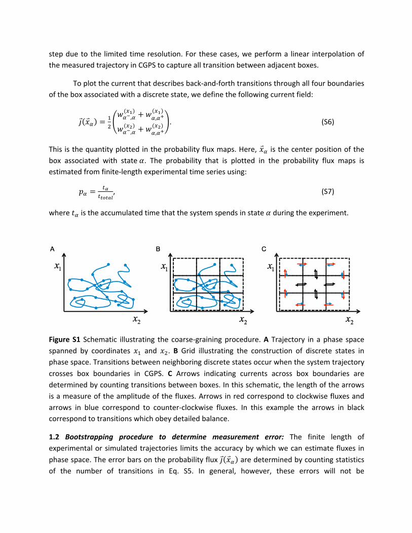
stepduetothe limitedtimeresolution.For thesecases,weperforma linear interpolationofthemeasuredtrajectoryinCGPStocapturealltransitionbetweenadjacentboxes.

Toplotthecurrentthatdescribesback-and-forthtransitionsthroughallfourboundariesoftheboxassociatedwithadiscretestate,wedefinethefollowingcurrentfield:

𝚥 𝑥! = !!

𝑤!!,!(!!) + 𝑤!,!!

!!

𝑤!!,!(!!) + 𝑤!,!!

(!!). (S6)

This isthequantityplottedintheprobabilityfluxmaps.Here,𝑥! isthecenterpositionofthebox associated with state 𝛼. The probability that is plotted in the probability flux maps isestimatedfromfinite-lengthexperimentaltimeseriesusing:

𝑝! =!!

!!"!#$, (S7)

where𝑡! istheaccumulatedtimethatthesystemspendsinstate𝛼duringtheexperiment.

FigureS1Schematic illustrating the coarse-grainingprocedure.A Trajectory in aphase spacespanned by coordinates 𝑥! and 𝑥!. BGrid illustrating the construction of discrete states inphasespace.Transitionsbetweenneighboringdiscretestatesoccurwhenthesystemtrajectorycrosses box boundaries in CGPS. C Arrows indicating currents across box boundaries aredeterminedbycountingtransitionsbetweenboxes.Inthisschematic,thelengthofthearrowsisameasureoftheamplitudeofthefluxes.Arrowsinredcorrespondtoclockwisefluxesandarrows in blue correspond to counter-clockwise fluxes. In this example the arrows in blackcorrespondtotransitionswhichobeydetailedbalance.

1.2 Bootstrapping procedure to determine measurement error: The finite length ofexperimentalorsimulatedtrajectories limits theaccuracybywhichwecanestimate fluxes inphasespace.Theerrorbarsontheprobabilityflux𝚥 𝑥! aredeterminedbycountingstatisticsof the number of transitions in Eq. S5. In general, however, these errors will not be

independent, reflecting correlations between in- andoutward transitions for a givenbox. Toestimate the error bars on 𝚥 𝑥! more precisely, we bootstrapped trajectories using theexperimentally measured or simulated trajectories. To perform this procedure, we firstdeterminethetransitionsbetweenstatesfromthedataanddefinedthefollowingarray

𝐴!"#" =

𝛼! 𝛼! 𝑡!,!𝛼! 𝛼! 𝑡!,!… … …𝛼! 𝛼!!! 𝑡!,!!!

. (S9)

Here,𝛼! and𝛼!!! are consecutively visited states, and 𝑡!,!!! is the amount of time spent in

state𝛼! beforetransitioningtostate𝛼!!!.Forexample,onecanestimatetherate𝑤!!,!(!!) from

thisusing:

𝑤!!,!(!!) = !

!!"!#$𝛿!!,!!!!𝛿!,!! − 𝛿!,!!𝛿!!,!!!!! . (S10)

Thestatementthatin-andoutwardtransitionsarecorrelatedmeansthatpairsoftermsinthissum are not independent. For instance, if there is a transition 𝛼! ⟶ 𝛼, contributing to a“count’’ in the first term under the sum, then it is likely that this event is followed by atransition𝛼 ⟶ 𝛼!,contributingtoa“count”inthesecondterm.Ifsuchcorrelationswerenotpresent (i.e., foraMarkoviansystem),wecouldconstructbootstraptrajectoriesbyrandomlypicking rows from 𝐴!"#" (Eq. s9). However, to capture the effects of pairwise correlationsbetween transitions on the accuracy with which we can estimate the fluxes, we bootstraptrajectories (with duration 𝑡!"!#$) by randomly picking consecutivepairs of rows from𝐴!"#".Empirically, we find that the estimated error bars reduce substantially by including pairwisecorrelations.Interestingly,thisindicatesthatoursystemsarenotentirelyMarkovian.Itisalsopossible to probe non-Markovian effects by the use of higher-order correlation functionsinvolvingthreeormoretimeintervals(40, 41).

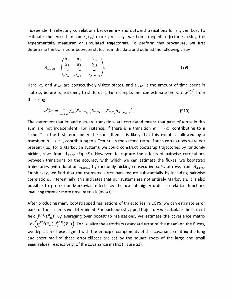
AfterproducingmanybootstrappedrealizationsoftrajectoriesinCGPS,wecanestimateerrorbarsforthecurrentswedetermined.Foreachbootstrappedtrajectorywecalculatethecurrentfield 𝚥(!") 𝑥! . By averaging over bootstrap realizations, we estimate the covariance matrix

Cov 𝑗!(!") 𝑥! , 𝑗!

(!") 𝑥! .Tovisualizetheerrorbars(standarderrorofthemean)onthefluxes,

wedepictanellipsealignedwiththeprinciplecomponentsofthiscovariancematrix;thelongand short radii of these error-ellipses are set by the square roots of the large and smalleigenvalues,respectively,ofthecovariancematrix(FigureS2).

FigureS2SchematicillustratingthedefinitionofthecurrentfieldinS6.Theflux(blackarrow)that we associate with a point at the center of a box is calculated by averaging theinward/outwardcurrentcontributions fromthefourboundaries (blueandredarrows)of thisbox.Theconfidence intervalsaredepictedaswhite,ellipticaldisks.Theaxesoftheseellipsesarealignedwiththeprinciplecomponentsof thiscovariancematrix,andtheir longandshortradii are set by the square roots of the large and small eigenvalues, respectively, of thecovariancematrix.

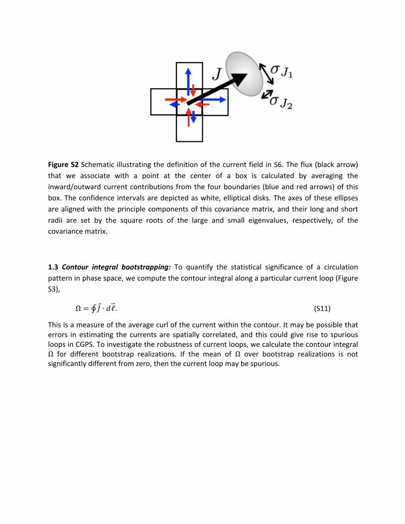
1.3 Contour integral bootstrapping: To quantify the statistical significance of a circulationpatterninphasespace,wecomputethecontourintegralalongaparticularcurrentloop(FigureS3),

Ω = 𝐽 ∙ 𝑑ℓ. (S11)

Thisisameasureoftheaveragecurlofthecurrentwithinthecontour.Itmaybepossiblethaterrors in estimating the currents are spatially correlated, and this could give rise to spuriousloopsinCGPS.Toinvestigatetherobustnessofcurrentloops,wecalculatethecontourintegralΩ for different bootstrap realizations. If the mean of Ω over bootstrap realizations is notsignificantlydifferentfromzero,thenthecurrentloopmaybespurious.

FigureS3:Schematicofcontourintegral.Redarrowscorrespondtoprobabilitycurrentvectors,theblue linedepicts thecontour integratedaround,and𝜃a representativeanglebetweenacurrentvectorandthecontour.

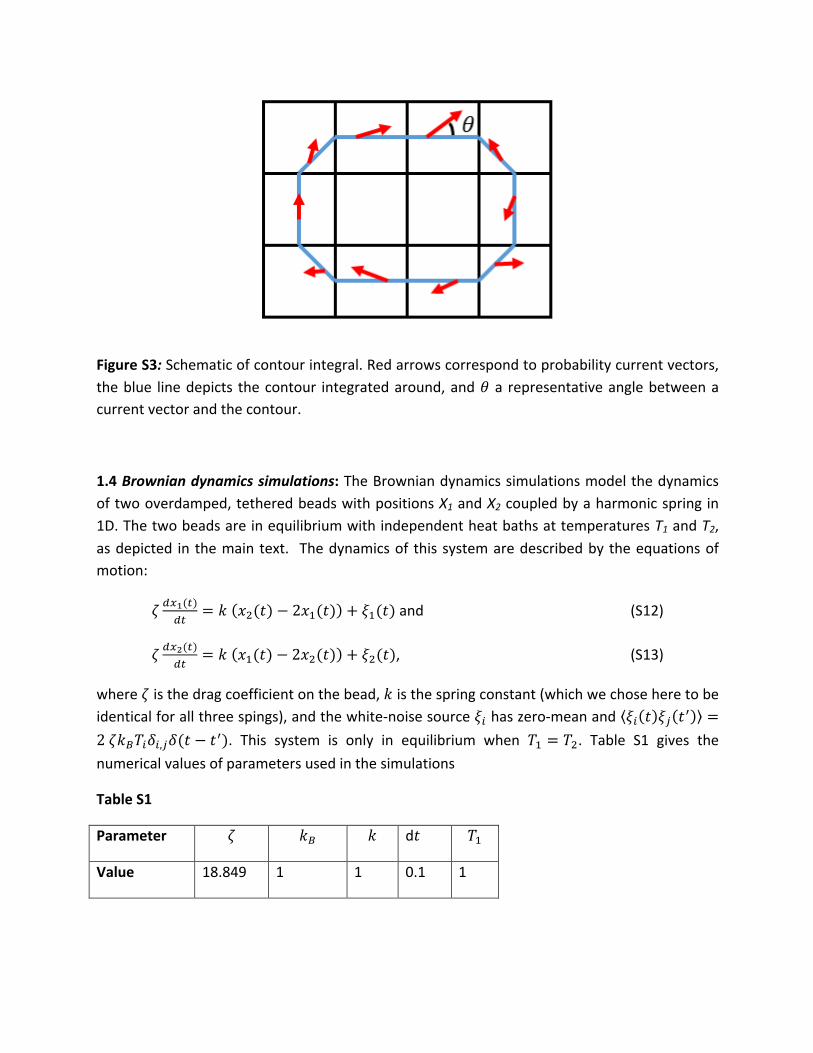
1.4Browniandynamicssimulations:TheBrowniandynamicssimulationsmodelthedynamicsoftwooverdamped,tetheredbeadswithpositionsX1andX2coupledbyaharmonicspringin1D.ThetwobeadsareinequilibriumwithindependentheatbathsattemperaturesT1andT2,asdepicted in themain text. Thedynamicsof thissystemaredescribedby theequationsofmotion:

𝜁 !!!(!)!"

= 𝑘 𝑥!(𝑡)− 2𝑥!(𝑡) + 𝜉!(𝑡)and (S12)

𝜁 !!!(!)!"

= 𝑘 𝑥!(𝑡)− 2𝑥!(𝑡) + 𝜉!(𝑡), (S13)

where𝜁isthedragcoefficientonthebead,𝑘isthespringconstant(whichwechoseheretobeidenticalforallthreespings),andthewhite-noisesource𝜉! haszero-meanand 𝜉! 𝑡 𝜉! 𝑡! =2 𝜁𝑘!𝑇!𝛿!,!𝛿(𝑡 − 𝑡!). This system is only in equilibrium when 𝑇! = 𝑇!. Table S1 gives thenumericalvaluesofparametersusedinthesimulations

TableS1

Parameter 𝜁 𝑘! 𝑘 d𝑡 𝑇!

Value 18.849 1 1 0.1 1

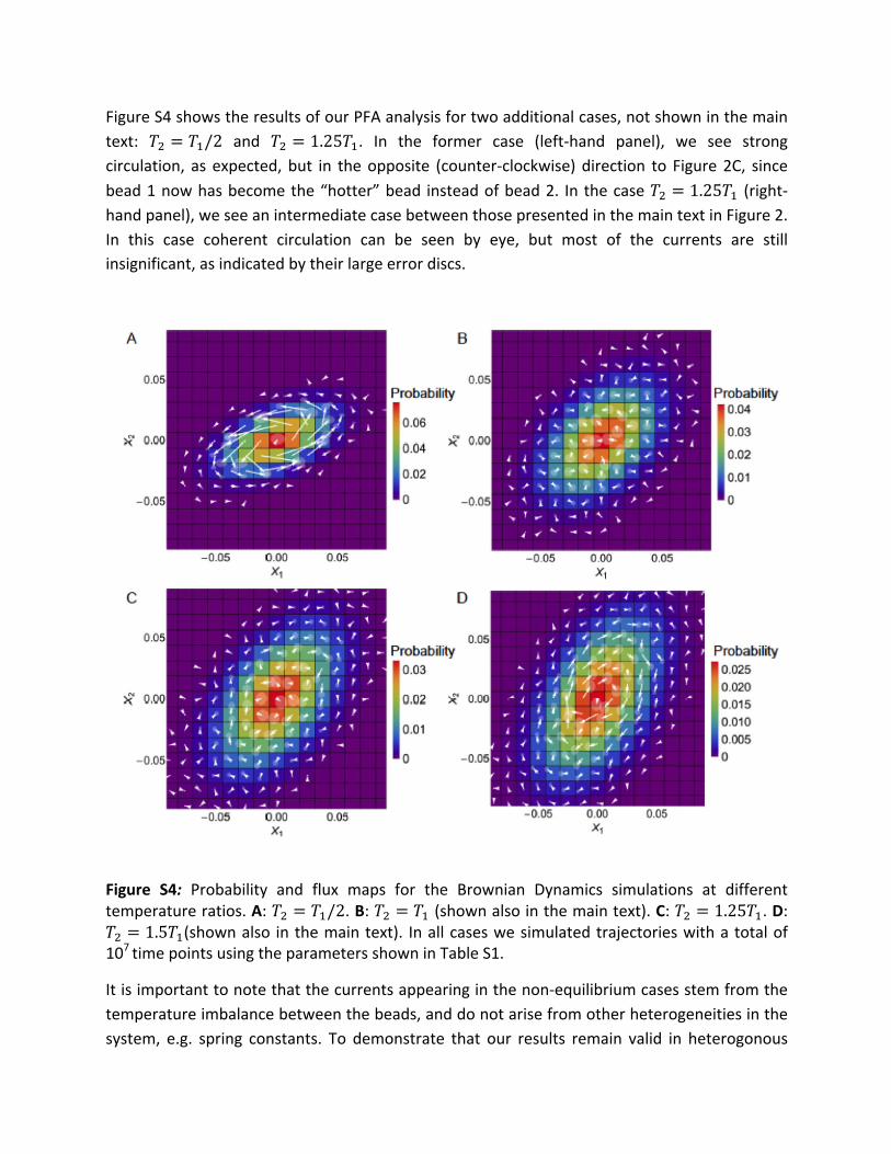
FigureS4showstheresultsofourPFAanalysisfortwoadditionalcases,notshowninthemaintext: 𝑇! = 𝑇!/2 and 𝑇! = 1.25𝑇!. In the former case (left-hand panel), we see strongcirculation, as expected,but in theopposite (counter-clockwise)direction to Figure2C, sincebead1nowhasbecomethe“hotter”bead insteadofbead2. In thecase𝑇! = 1.25𝑇! (right-handpanel),weseeanintermediatecasebetweenthosepresentedinthemaintextinFigure2.In this case coherent circulation can be seen by eye, but most of the currents are stillinsignificant,asindicatedbytheirlargeerrordiscs.

Figure S4: Probability and flux maps for the Brownian Dynamics simulations at differenttemperatureratios.A:𝑇! = 𝑇!/2.B:𝑇! = 𝑇!(shownalsointhemaintext).C:𝑇! = 1.25𝑇!.D:𝑇! = 1.5𝑇!(shownalso inthemaintext). Inallcaseswesimulatedtrajectorieswithatotalof107timepointsusingtheparametersshowninTableS1.

Itisimportanttonotethatthecurrentsappearinginthenon-equilibriumcasesstemfromthetemperatureimbalancebetweenthebeads,anddonotarisefromotherheterogeneitiesinthesystem, e.g. spring constants. To demonstrate that our results remain valid in heterogonous

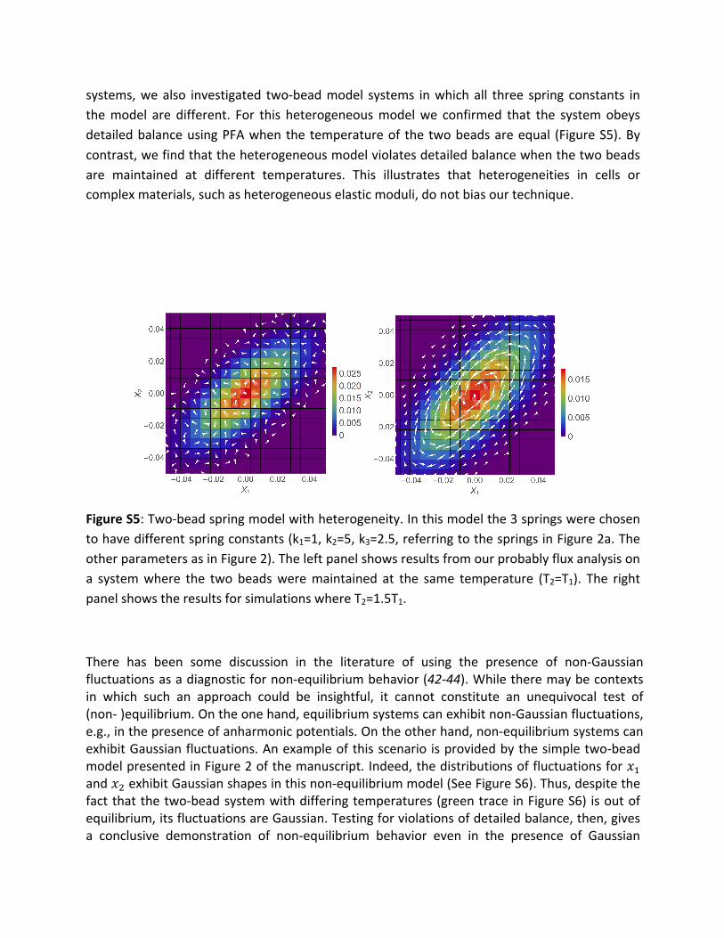
systems,wealso investigated two-beadmodel systems inwhichall three spring constants inthemodel are different. For this heterogeneousmodelwe confirmed that the systemobeysdetailedbalanceusingPFAwhenthetemperatureof thetwobeadsareequal (FigureS5).Bycontrast,wefindthattheheterogeneousmodelviolatesdetailedbalancewhenthetwobeadsare maintained at different temperatures. This illustrates that heterogeneities in cells orcomplexmaterials,suchasheterogeneouselasticmoduli,donotbiasourtechnique.

FigureS5:Two-beadspringmodelwithheterogeneity.Inthismodelthe3springswerechosentohavedifferentspringconstants(k1=1,k2=5,k3=2.5,referringtothespringsinFigure2a.TheotherparametersasinFigure2).Theleftpanelshowsresultsfromourprobablyfluxanalysisona systemwhere the two beadsweremaintained at the same temperature (T2=T1). The rightpanelshowstheresultsforsimulationswhereT2=1.5T1.

There has been some discussion in the literature of using the presence of non-Gaussianfluctuationsasadiagnosticfornon-equilibriumbehavior(42-44).Whiletheremaybecontextsin which such an approach could be insightful, it cannot constitute an unequivocal test of(non- )equilibrium.Ontheonehand,equilibriumsystemscanexhibitnon-Gaussianfluctuations,e.g.,inthepresenceofanharmonicpotentials.Ontheotherhand,non-equilibriumsystemscanexhibitGaussianfluctuations.Anexampleofthisscenario isprovidedbythesimpletwo-beadmodelpresentedinFigure2ofthemanuscript.Indeed,thedistributionsoffluctuationsfor𝑥!and𝑥!exhibitGaussianshapesinthisnon-equilibriummodel(SeeFigureS6).Thus,despitethefactthatthetwo-beadsystemwithdifferingtemperatures(greentrace inFigureS6) isoutofequilibrium,itsfluctuationsareGaussian.Testingforviolationsofdetailedbalance,then,givesa conclusive demonstration of non-equilibrium behavior even in the presence of Gaussian

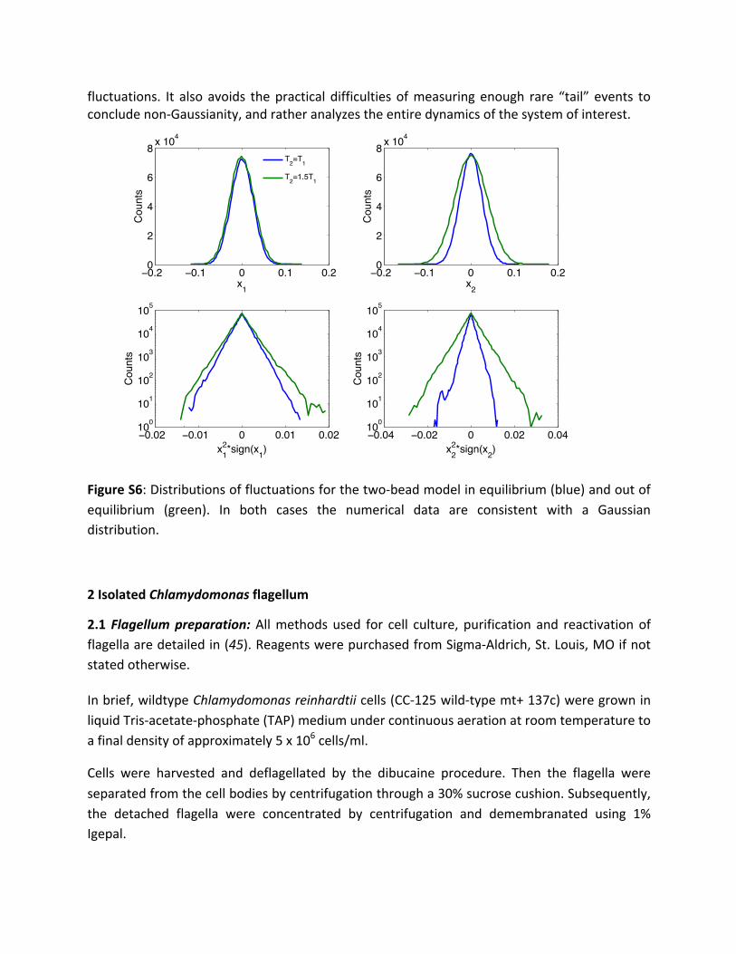
fluctuations. It also avoids thepractical difficultiesofmeasuringenough rare “tail” events toconcludenon-Gaussianity,andratheranalyzestheentiredynamicsofthesystemofinterest.

FigureS6:Distributionsoffluctuationsforthetwo-beadmodelinequilibrium(blue)andoutofequilibrium (green). In both cases the numerical data are consistent with a Gaussiandistribution.

2IsolatedChlamydomonasflagellum

2.1Flagellumpreparation:Allmethodsused for cell culture, purification and reactivationofflagellaaredetailedin(45).ReagentswerepurchasedfromSigma-Aldrich,St.Louis,MOifnotstatedotherwise.

Inbrief,wildtypeChlamydomonasreinhardtiicells(CC-125wild-typemt+137c)weregrowninliquidTris-acetate-phosphate(TAP)mediumundercontinuousaerationatroomtemperaturetoafinaldensityofapproximately5x106cells/ml.

Cells were harvested and deflagellated by the dibucaine procedure. Then the flagella wereseparatedfromthecellbodiesbycentrifugationthrougha30%sucrosecushion.Subsequently,the detached flagella were concentrated by centrifugation and demembranated using 1%Igepal.

−0.2 −0.1 0 0.1 0.20

2

4

6

8 x 104

x1

Cou

nts

−0.2 −0.1 0 0.1 0.20

2

4

6

8 x 104

x2

Cou

nts

−0.02 −0.01 0 0.01 0.02100

101

102

103

104

105

x12*sign(x1)

Cou

nts

−0.04 −0.02 0 0.02 0.04100

101

102

103

104

105

x22*sign(x2)

Cou

nts

T2=T1

T2=1.5T1

Thebufferused fordemembranationwasHMDEK (30mMHEPES,5mMMgSO4,1mMDTT,and1mMEGTA,50mMK-acetate,titratedtopH7.4withKOH).Duringthedemembranationandforallsubsequentsteps0.2mMPefablocwasaddedtoallsolutions.

Thedemembranatedflagellawerereactivated inabufferHMDEKbufferaugmentedwith,1%PEG(20k)1mMATP,1mMDTT,10units/mlcreatinekinaseand6.4mMcreatinephosphate.

2.2Imagingchambers:Flowchambersweremadefromdouble-sticktapeandcleanedglass(easy-cleanprocedure(46))resultinginachamberwithaheightof~100µmandawidthof3mm.First,surfaceswereblockedwitha2mg/mlcaseinsolutionfor5minutes,thenthesamplewasplacedintothechambers.Finally,thechambersweresealedwithVALAP(1:1:1vasoline:lanolin:parafin).

2.3Microscopy: Beating flagella were visualized using phase-contrast microscopy on a ZeissAxiovert200invertedmicroscope.Themicroscopewasequippedwitha100xPlan-NeofluarNA1.3PH3oilobjective,aZeissoilphase-contrastcondenser(NA1.4).Additionallya1.6xOptovarlenswasusedtoenhancesamplemagnification.Thesampleswereilluminatedusinga100-Wtungstenlamp.Imageswereacquiredataframerateof1000fps(framespersecond)usingahigh-speedCMOScamera (FastcamSA3,Photron)withaneffectivepixel sizeof106.25nmx106.25nm.

2.4Flagellum trackingandnormalmodes:Thebackboneof the flagellumwas trackedusingFluorescence ImageEvaluationSoftware forTrackingandAnalysis (FIESTA) (47). The shapeof

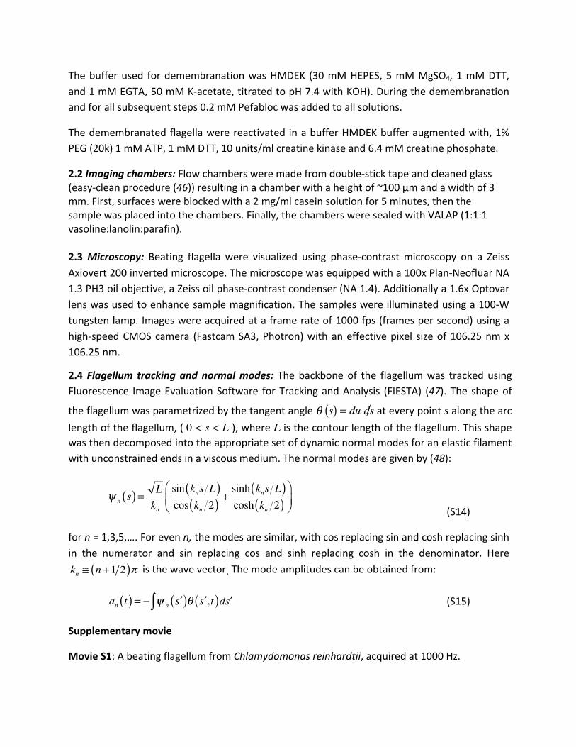
theflagellumwasparametrizedbythetangentangleθ (s) = du dsateverypointsalongthe arclengthoftheflagellum,( 0 < s < L ),whereListhecontourlengthoftheflagellum.Thisshapewasthendecomposedintotheappropriatesetofdynamicnormalmodesforanelasticfilamentwithunconstrainedendsinaviscousmedium.Thenormalmodesaregivenby(48):

ψ n s( ) = Lkn

sin kns L( )cos kn 2( ) +

sinh kns L( )cosh kn 2( )

⎛

⎝⎜⎞

⎠⎟ (S14)

forn=1,3,5,….Forevenn,themodesaresimilar,withcosreplacingsinandcoshreplacingsinhin the numerator and sin replacing cos and sinh replacing cosh in the denominator. Herekn ≅ n +1 2( )π isthewavevector.Themodeamplitudescanbeobtainedfrom:

an t( ) = − ψ n ′s( )θ ′s ,t( )d ′s∫ (S15)

Supplementarymovie

MovieS1:AbeatingflagellumfromChlamydomonasreinhardtii,acquiredat1000Hz.

3Cilium

3.1Cellculture:Madin-Darbycaninekidney(MDCK-II)cells(akindgiftfromAndreasJanshoff)were cultured in Minimum Essential Medium with 2 mM L-glutamine, 1% penicillin-streptomycin, and10% fetalbovine serumadded.Cellsweregrown to confluenceonpoly-L-lysine-coatedpolycarbonatemembranes(PCMs),andexperimentswereperformed1-2daysafterfullconfluence(5-7daysafterseeding).

3.2Blebbistatintreatment:Blebbistatinwasaddedtotheculturemediumofconfluentcellstoaconcentrationof50μMoftheactive(-)enantiomer(100μMofracemicsolution,CalBiochem,203389). The cells were incubated in the blebbistatin solution at 37°C for 30minutes, afterwhichtheyweremountedwithblebbistatin-containingmediuminviewingchambersforvideo-trackingexperiments.

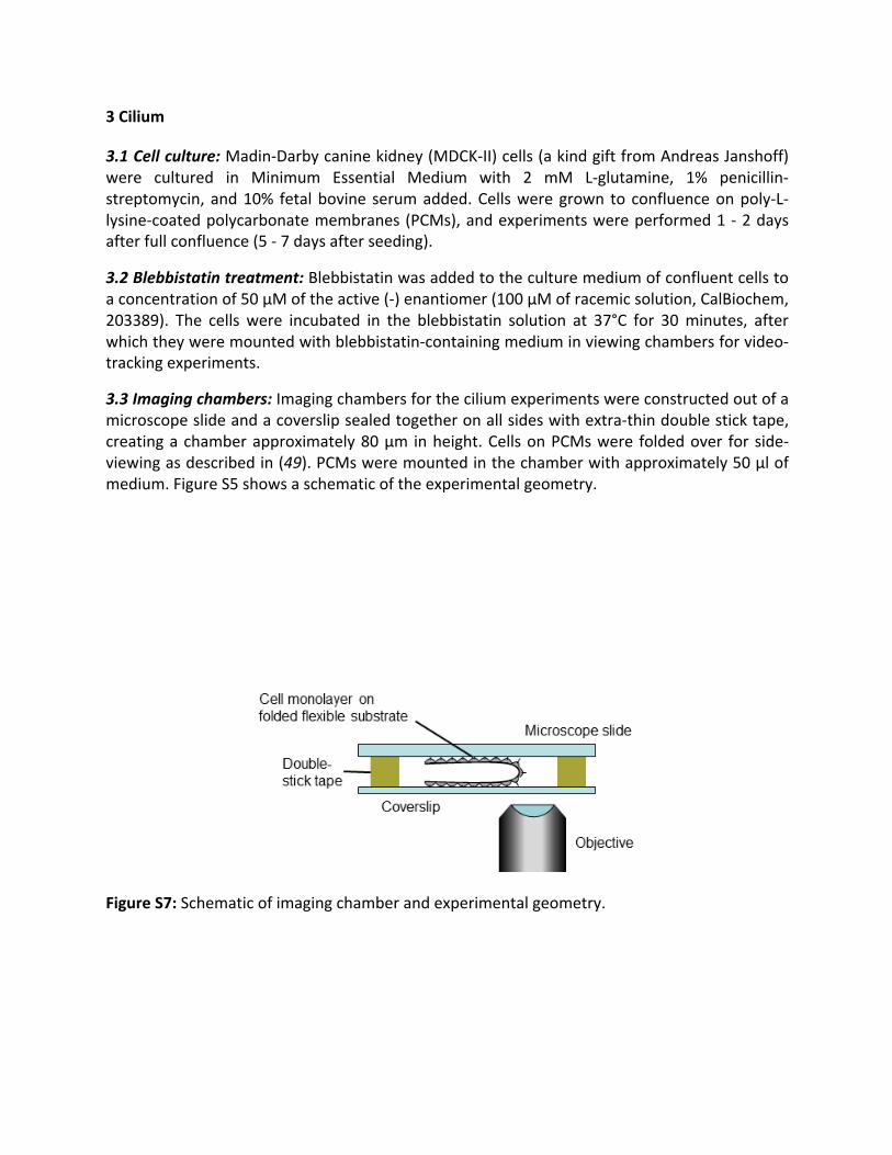
3.3Imagingchambers:Imagingchambersfortheciliumexperimentswereconstructedoutofamicroscopeslideandacoverslipsealedtogetheronallsideswithextra-thindoublesticktape,creatingachamberapproximately80μm inheight.CellsonPCMswere foldedover forside-viewingasdescribedin(49).PCMsweremountedinthechamberwithapproximately50μlofmedium.FigureS5showsaschematicoftheexperimentalgeometry.

FigureS7:Schematicofimagingchamberandexperimentalgeometry.

3.4Microscopy:Primaryciliumexperimentswereperformedusingacustom-builtDIC/optical-trapping setup described elsewhere (50). Imageswere acquiredwith anMTI VE1000 analogcamera(DAGE-MTI,MichiganCity,IN)atarateof25Hzandreadoutviaaframegrabbercardandacustom-writtenLabViewVI.

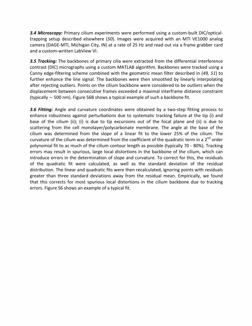
3.5Tracking:Thebackbonesofprimaryciliawereextractedfromthedifferentialinterferencecontrast(DIC)micrographsusingacustomMATLABalgorithm.BackbonesweretrackedusingaCannyedge-filteringschemecombinedwiththegeometricmeanfilterdescribedin(49,51)tofurtherenhance the line signal. Thebackboneswere then smoothedby linearly interpolatingafterrejectingoutliers.Pointsontheciliumbackbonewereconsideredtobeoutlierswhenthedisplacementbetweenconsecutiveframesexceededamaximalinterframedistanceconstraint(typically~500nm).FigureS6Bshowsatypicalexampleofsuchabackbonefit.

3.6 Fitting: Angle and curvature coordinates were obtained by a two-step fitting process toenhance robustnessagainstperturbationsdue tosystematic tracking failureat the tip (i)andbase of the cilium (ii); (i) is due to tip excursions out of the focal plane and (ii) is due toscattering from the cell monolayer/polycarbonate membrane. The angle at the base of thecilium was determined from the slope of a linear fit to the lower 25% of the cilium. Thecurvatureoftheciliumwasdeterminedfromthecoefficientofthequadratictermina2ndorderpolynomialfittoasmuchoftheciliumcontourlengthaspossible(typically70-80%).Trackingerrorsmayresult inspurious, large localdistortions in thebackboneof thecilium,whichcanintroduceerrorsinthedeterminationofslopeandcurvature.Tocorrectforthis,theresidualsof the quadratic fit were calculated, as well as the standard deviation of the residualdistribution.Thelinearandquadraticfitswerethenrecalculated,ignoringpointswithresidualsgreater than three standard deviations away from the residualmean. Empirically, we foundthat this corrects formost spurious local distortions in the cilium backbone due to trackingerrors.FigureS6showsanexampleofatypicalfit.

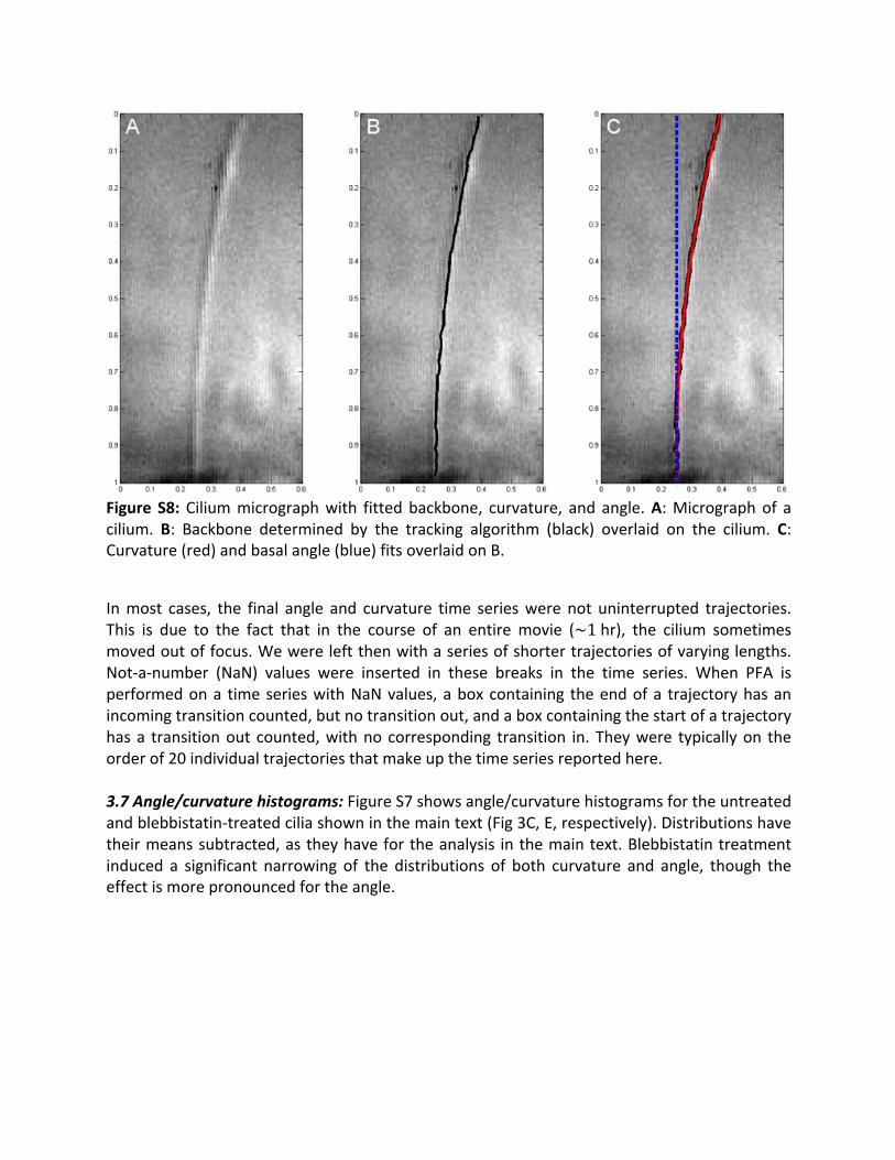
Figure S8:Ciliummicrographwith fittedbackbone, curvature, and angle.A:Micrographof acilium. B: Backbone determined by the tracking algorithm (black) overlaid on the cilium. C:Curvature(red)andbasalangle(blue)fitsoverlaidonB.

Inmost cases, the final angle and curvature time serieswere not uninterrupted trajectories.This is due to the fact that in the course of an entiremovie (~1 hr), the cilium sometimesmovedoutoffocus.Wewereleftthenwithaseriesofshortertrajectoriesofvaryinglengths.Not-a-number (NaN) values were inserted in these breaks in the time series. When PFA isperformedona timeserieswithNaNvalues,aboxcontaining theendofa trajectoryhasanincomingtransitioncounted,butnotransitionout,andaboxcontainingthestartofatrajectoryhasa transitionout counted,withnocorresponding transition in.Theywere typicallyon theorderof20individualtrajectoriesthatmakeupthetimeseriesreportedhere.3.7Angle/curvaturehistograms:FigureS7showsangle/curvaturehistogramsfortheuntreatedandblebbistatin-treatedciliashowninthemaintext(Fig3C,E,respectively).Distributionshavetheirmeanssubtracted,astheyhavefortheanalysis inthemaintext.Blebbistatintreatmentinduced a significant narrowing of the distributions of both curvature and angle, though theeffectismorepronouncedfortheangle.

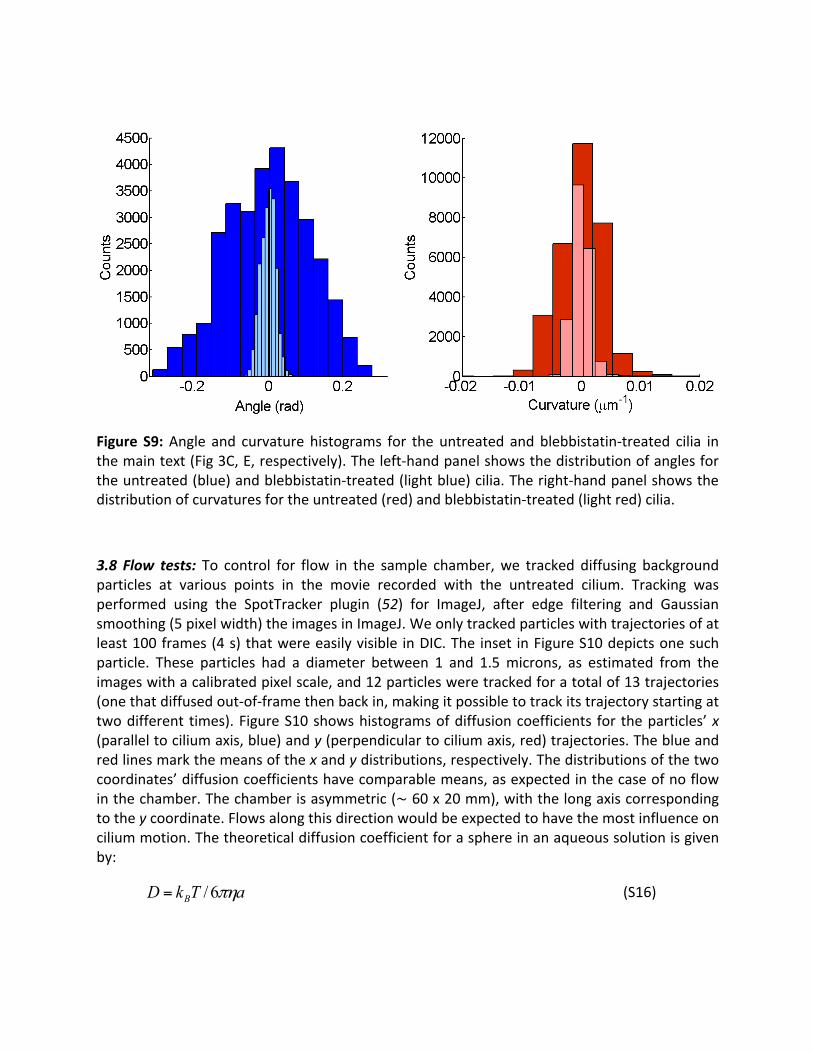
Figure S9:Angle and curvature histograms for the untreated andblebbistatin-treated cilia inthemaintext(Fig3C,E,respectively).Theleft-handpanelshowsthedistributionofanglesfortheuntreated(blue)andblebbistatin-treated(lightblue)cilia.Theright-handpanelshowsthedistributionofcurvaturesfortheuntreated(red)andblebbistatin-treated(lightred)cilia.

3.8 Flow tests:To control for flow in the sample chamber,we tracked diffusing backgroundparticles at various points in the movie recorded with the untreated cilium. Tracking wasperformed using the SpotTracker plugin (52) for ImageJ, after edge filtering and Gaussiansmoothing(5pixelwidth)theimagesinImageJ.Weonlytrackedparticleswithtrajectoriesofatleast100frames(4s)thatwereeasilyvisible inDIC.The inset inFigureS10depictsonesuchparticle. These particles had a diameter between 1 and 1.5microns, as estimated from theimageswithacalibratedpixelscale,and12particlesweretrackedforatotalof13trajectories(onethatdiffusedout-of-framethenbackin,makingitpossibletotrackitstrajectorystartingattwodifferent times).FigureS10showshistogramsofdiffusioncoefficients for theparticles’x(paralleltociliumaxis,blue)andy(perpendiculartociliumaxis,red)trajectories.Theblueandredlinesmarkthemeansofthexandydistributions,respectively.Thedistributionsofthetwocoordinates’diffusioncoefficientshavecomparablemeans,asexpectedinthecaseofnoflowinthechamber.Thechamberisasymmetric(~60x20mm),withthelongaxiscorrespondingtotheycoordinate.Flowsalongthisdirectionwouldbeexpectedtohavethemostinfluenceonciliummotion.Thetheoreticaldiffusioncoefficientforasphereinanaqueoussolutionisgivenby:

(S16)aTkD B πη6/=

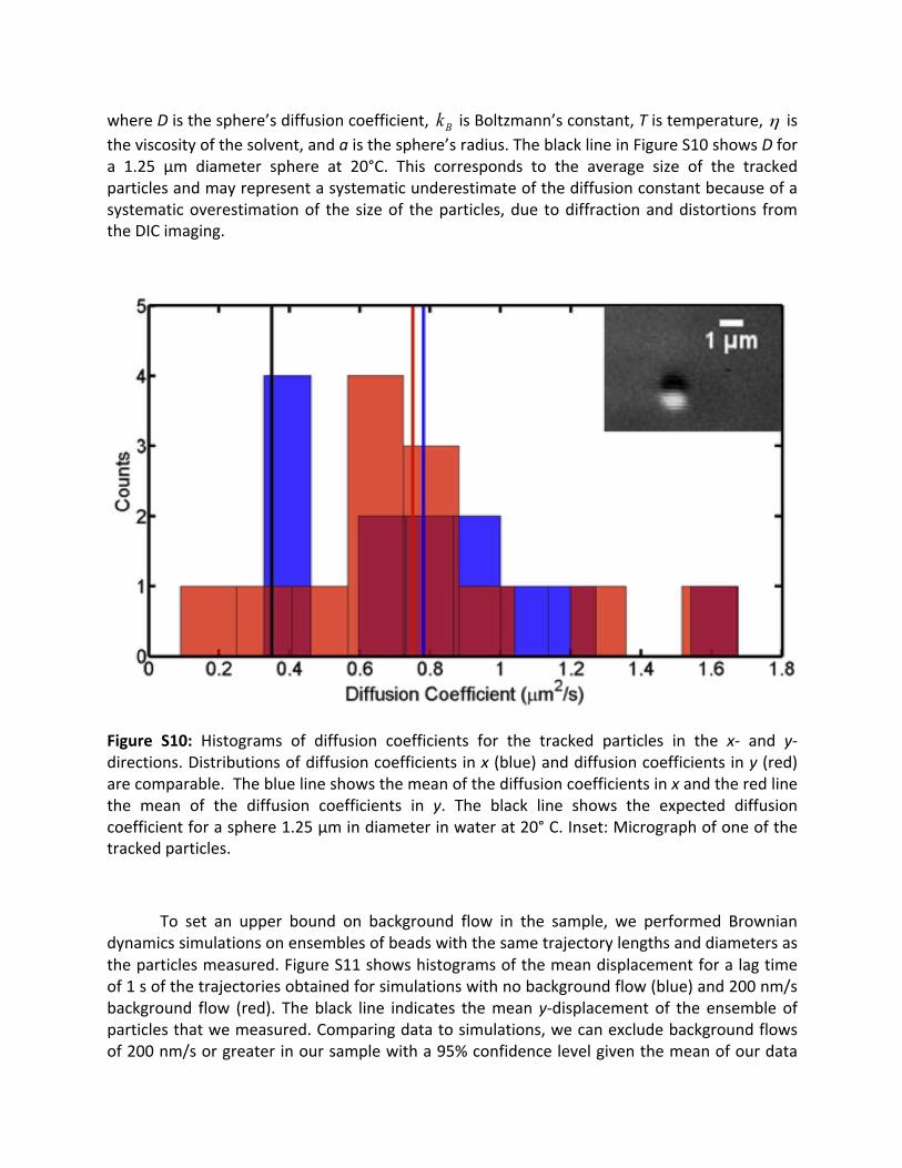
whereDisthesphere’sdiffusioncoefficient, isBoltzmann’sconstant,Tistemperature, istheviscosityofthesolvent,andaisthesphere’sradius.TheblacklineinFigureS10showsDfora 1.25 µm diameter sphere at 20°C. This corresponds to the average size of the trackedparticlesandmayrepresentasystematicunderestimateofthediffusionconstantbecauseofasystematicoverestimationof the sizeof theparticles,due todiffractionanddistortions fromtheDICimaging.

Figure S10: Histograms of diffusion coefficients for the tracked particles in the x- and y-directions.Distributionsofdiffusioncoefficientsinx(blue)anddiffusioncoefficientsiny(red)arecomparable.Thebluelineshowsthemeanofthediffusioncoefficientsinxandtheredlinethe mean of the diffusion coefficients in y. The black line shows the expected diffusioncoefficientforasphere1.25µmindiameterinwaterat20°C.Inset:Micrographofoneofthetrackedparticles.

To set an upper bound on background flow in the sample, we performed Browniandynamicssimulationsonensemblesofbeadswiththesametrajectorylengthsanddiametersastheparticlesmeasured.FigureS11showshistogramsofthemeandisplacementforalagtimeof1softhetrajectoriesobtainedforsimulationswithnobackgroundflow(blue)and200nm/sbackground flow (red). Theblack line indicates themeany-displacementof the ensembleofparticlesthatwemeasured.Comparingdatatosimulations,wecanexcludebackgroundflowsof200nm/sorgreaterinoursamplewitha95%confidencelevelgiventhemeanofourdata

Bk η

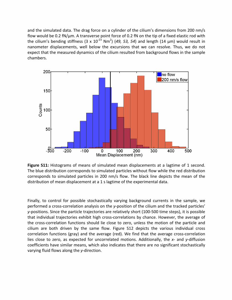
andthesimulateddata.Thedragforceonacylinderofthecilium’sdimensionsfrom200nm/sflowwouldbe0.2fN/µm.Atransversepointforceof0.2fNonthetipofafixedelasticrodwiththe cilium’sbending stiffness (3 x10-23Nm2) (49,53,54) and length (14µm)would result innanometer displacements, well below the excursions that we can resolve. Thus, we do notexpectthatthemeasureddynamicsoftheciliumresultedfrombackgroundflowsinthesamplechambers.

FigureS11:Histogramsofmeansof simulatedmeandisplacementsata lagtimeof1 second.Thebluedistributioncorrespondstosimulatedparticleswithoutflowwhilethereddistributioncorresponds to simulatedparticles in 200nm/s flow. Theblack line depicts themeanof thedistributionofmeandisplacementata1slagtimeoftheexperimentaldata.

Finally, to control for possible stochastically varying background currents in the sample, weperformedacross-correlationanalysisonthey-positionoftheciliumandthetrackedparticles’y-positions.Sincetheparticletrajectoriesarerelativelyshort(100-500timesteps),itispossiblethat individual trajectoriesexhibithighcross-correlationsbychance.However, theaverageofthecross-correlation functions should lie close to zero,unless themotionof theparticleandcilium are both driven by the same flow. Figure S12 depicts the various individual crosscorrelation functions (gray)andtheaverage (red).We find that theaveragecross-correlationlies close to zero, as expected for uncorrelatedmotions. Additionally, the x- and y-diffusioncoefficientshavesimilarmeans,whichalsoindicatesthattherearenosignificantstochasticallyvaryingfluidflowsalongthey-direction.

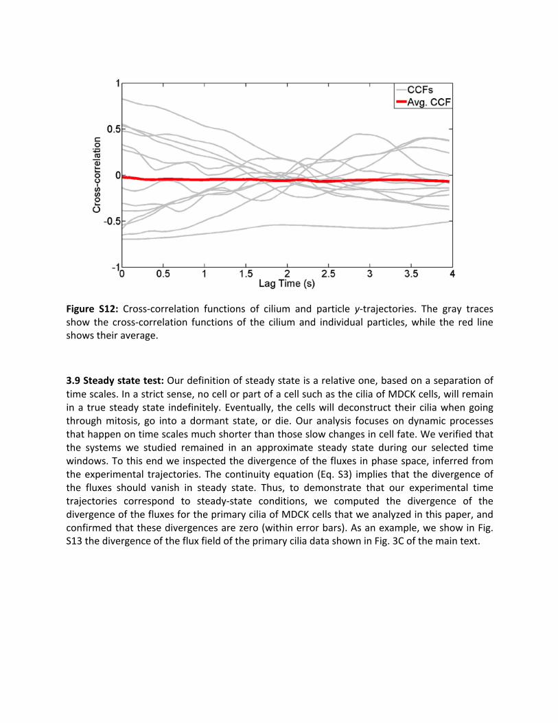
Figure S12: Cross-correlation functions of cilium and particle y-trajectories. The gray tracesshow the cross-correlation functions of the ciliumand individual particles,while the red lineshowstheiraverage.

3.9Steadystatetest:Ourdefinitionofsteadystateisarelativeone,basedonaseparationoftimescales.Inastrictsense,nocellorpartofacellsuchastheciliaofMDCKcells,willremainina truesteadystate indefinitely.Eventually, thecellswilldeconstruct theirciliawhengoingthroughmitosis, go into a dormant state, or die.Our analysis focuses on dynamic processesthathappenontimescalesmuchshorterthanthoseslowchangesincellfate.Weverifiedthatthe systems we studied remained in an approximate steady state during our selected timewindows.Tothisendweinspectedthedivergenceofthefluxesinphasespace,inferredfromtheexperimental trajectories.Thecontinuityequation (Eq.S3) implies that thedivergenceofthe fluxes should vanish in steady state. Thus, to demonstrate that our experimental timetrajectories correspond to steady-state conditions, we computed the divergence of thedivergenceofthefluxesfortheprimaryciliaofMDCKcellsthatweanalyzedinthispaper,andconfirmedthatthesedivergencesarezero(withinerrorbars).Asanexample,weshowinFig.S13thedivergenceofthefluxfieldoftheprimaryciliadatashowninFig.3Cofthemaintext.

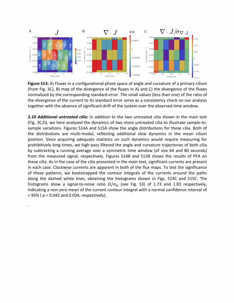
FigureS13:A)Fluxesinaconfigurationalphasespaceofangleandcurvatureofaprimarycilium(fromFig.3C),B)mapofthedivergenceofthefluxesinA)andC)thedivergenceofthefluxesnormalizedbythecorrespondingstandarderror.Thesmallvalues(lessthanone)oftheratioofthedivergenceofthecurrenttoitsstandarderrorserveasaconsistencycheckonouranalysistogetherwiththeabsenceofsignificantdriftofthesystemovertheobservedtimewindow.

3.10Additionaluntreatedcilia: Inadditiontothetwountreatedciliashowninthemaintext(Fig.3C,D),wehereanalyzedthedynamicsoftwomoreuntreatedciliatoillustratesample-to-samplevariations.FiguresS14AandS15Ashowtheangledistributionsforthesecilia.Bothofthe distributions are multi-modal, reflecting additional slow dynamics in the mean ciliumposition. Since acquiring adequate statistics on such dynamics would require measuring forprohibitivelylongtimes,wehigh-passfilteredtheangleandcurvaturetrajectoriesofbothciliaby subtractinga runningaverageovera symmetric timewindow (of size64and80 seconds)from themeasured signal, respectively. Figures S14B and S15B shows the results of PFA onthesecilia.Asinthecaseoftheciliapresentedinthemaintext,significantcurrentsarepresentineachcase.Clockwisecurrentsareapparentinbothofthefluxmaps.Totestthesignificanceof these patterns, we bootstrapped the contour integrals of the currents around the pathsalong the dashed white lines, obtaining the histograms shown in Figs. S14C and S15C. Thehistograms show a signal-to-noise ratio Ω/σ! (see Fig. S3) of 1.73 and 1.83 respectively,indicatinganon-zeromeanofthecurrentcontourintegralwithanormalconfidenceintervalof>95%(p=0.042and0.034,respectively).

.

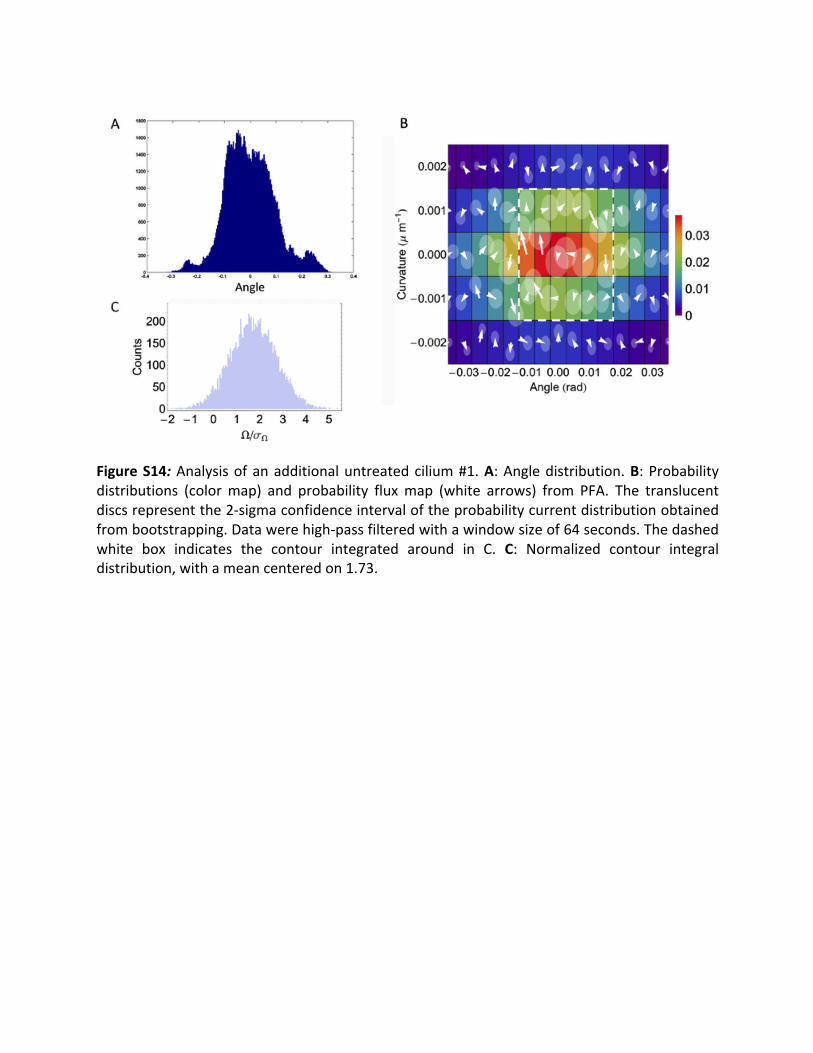
FigureS14:Analysisofanadditionaluntreatedcilium#1.A:Angledistribution.B:Probabilitydistributions (colormap) and probability fluxmap (white arrows) from PFA. The translucentdiscsrepresentthe2-sigmaconfidenceintervaloftheprobabilitycurrentdistributionobtainedfrombootstrapping.Datawerehigh-passfilteredwithawindowsizeof64seconds.Thedashedwhite box indicates the contour integrated around in C. C: Normalized contour integraldistribution,withameancenteredon1.73.

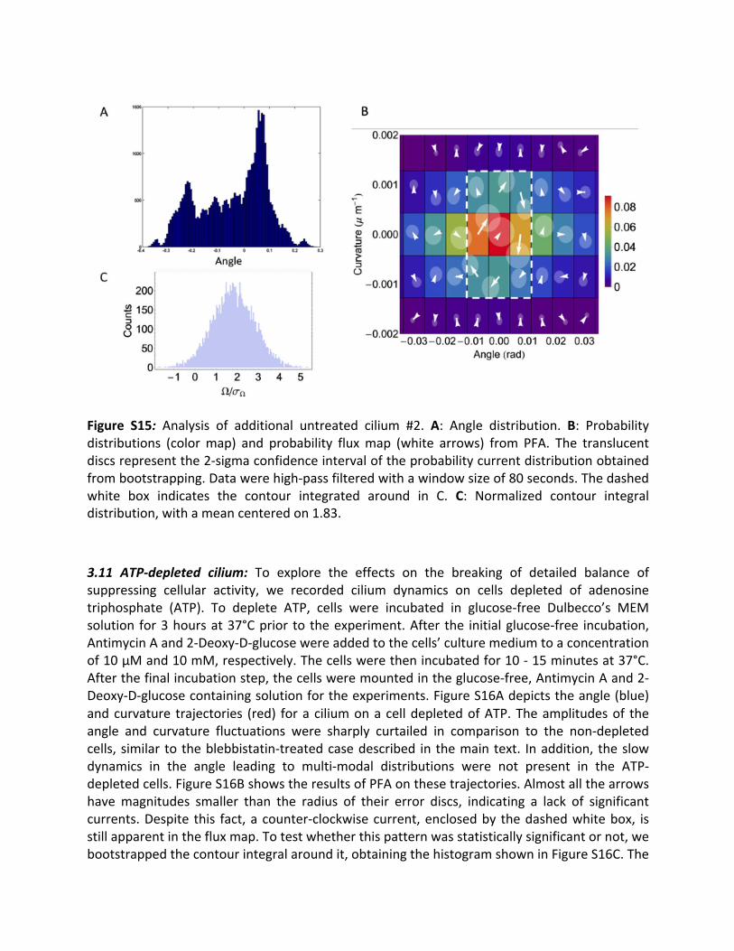
Figure S15: Analysis of additional untreated cilium #2. A: Angle distribution. B: Probabilitydistributions (colormap) and probability fluxmap (white arrows) from PFA. The translucentdiscsrepresentthe2-sigmaconfidenceintervaloftheprobabilitycurrentdistributionobtainedfrombootstrapping.Datawerehigh-passfilteredwithawindowsizeof80seconds.Thedashedwhite box indicates the contour integrated around in C. C: Normalized contour integraldistribution,withameancenteredon1.83.

3.11 ATP-depleted cilium: To explore the effects on the breaking of detailed balance ofsuppressing cellular activity, we recorded cilium dynamics on cells depleted of adenosinetriphosphate (ATP). To deplete ATP, cells were incubated in glucose-free Dulbecco’s MEMsolution for3hoursat37°Cprior to theexperiment.After the initialglucose-free incubation,AntimycinAand2-Deoxy-D-glucosewereaddedtothecells’culturemediumtoaconcentrationof10μMand10mM,respectively.Thecellswerethenincubatedfor10-15minutesat37°C.Afterthefinalincubationstep,thecellsweremountedintheglucose-free,AntimycinAand2-Deoxy-D-glucosecontainingsolutionfortheexperiments.FigureS16Adepictstheangle(blue)andcurvature trajectories (red) foraciliumonacelldepletedofATP.Theamplitudesof theangle and curvature fluctuations were sharply curtailed in comparison to the non-depletedcells,similar totheblebbistatin-treatedcasedescribed inthemaintext. Inaddition, theslowdynamics in the angle leading to multi-modal distributions were not present in the ATP-depletedcells.FigureS16BshowstheresultsofPFAonthesetrajectories.Almostallthearrowshavemagnitudes smaller than the radius of their error discs, indicating a lack of significantcurrents.Despite this fact,acounter-clockwisecurrent,enclosedby thedashedwhitebox, isstillapparentinthefluxmap.Totestwhetherthispatternwasstatisticallysignificantornot,webootstrappedthecontourintegralaroundit,obtainingthehistogramshowninFigureS16C.The

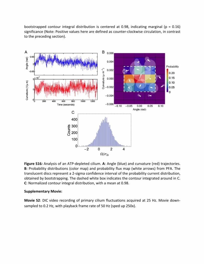
bootstrapped contour integral distribution is centered at 0.98, indicatingmarginal (p = 0.16)significance(Note:Positivevaluesherearedefinedascounter-clockwisecirculation,incontrasttotheprecedingsection).

FigureS16:AnalysisofanATP-depletedcilium.A:Angle(blue)andcurvature(red)trajectories.B:Probabilitydistributions(colormap)andprobabilityfluxmap(whitearrows)fromPFA.Thetranslucentdiscsrepresenta2-sigmaconfidenceintervaloftheprobabilitycurrentdistribution,obtainedbybootstrapping.ThedashedwhiteboxindicatesthecontourintegratedaroundinC.C:Normalizedcontourintegraldistribution,withameanat0.98.

SupplementaryMovie:

MovieS2:DICvideorecordingofprimaryciliumfluctuationsacquiredat25Hz.Moviedown-sampledto0.2Hz,withplaybackframerateof50Hz(spedup250x).

4Microtubulefluctuations,equilibriumcontrol

4.1Microtubule preparation:Microtubules were polymerized at 37°C in BRB80 buffer (80mMK-Pipes, pH 6.8, 1mMEGTA, 1mMMgCl2) augmentedwith 5mMMgCl2, 1mMGTP,20µMunlabeledTubulinand5%DMSOfor40min.MicrotubuleswerethenspunintoapelletinanBeckmanntabletopairfugefor5minat25psi.Thepelletwasresuspended in100µlofBRB80buffercontaining10µMtaxol,thatwasfilteredusinga0.22µmfilter.AllreagentswerepurchasedfromSigmaAldrich.

4.2Samplechambers:Forimaging,freshlyresuspendedmicrotubuleswerediluted40xintaxolcontainingBRB80bufferaugmentedwith0.1mg/mlCasein.7µlofthissolutionwerepipettedontoamicroscopyslideandcoveredwitha22x22mmcoverglass. Thechamberheightwasbetween 1-3 µm and it wassealed using Valap, a 1:1:1 mixture of lanolin, paraffin, andpetroleum jelly, heated to 70°C. The glasswaspre-cleanedby 15min sonication steps in 5%Mucasol solution and ethanolfollowed by an extensive washing step using filtered double-distilledwaterandadryingstepusingpressurizednitrogen.

4.3 Microscopy: Microtubules were visualized by darkfield microscopy in aNikon EclipseTimicroscope using aNikon Plan Fluor 100x, NA 0.5-1.3 lens and a Nikon oil darkfieldcondenser NA 1.43-1.20. The sample was illuminated with a Sola light engine(lumencor). Fluctuatingmicrotubuleswere imaged for10minusingaAndorZyla4.2 camera(2x2binning).Theexposuretimewas5ms,theeffectivepixel-size128nm/pixel.

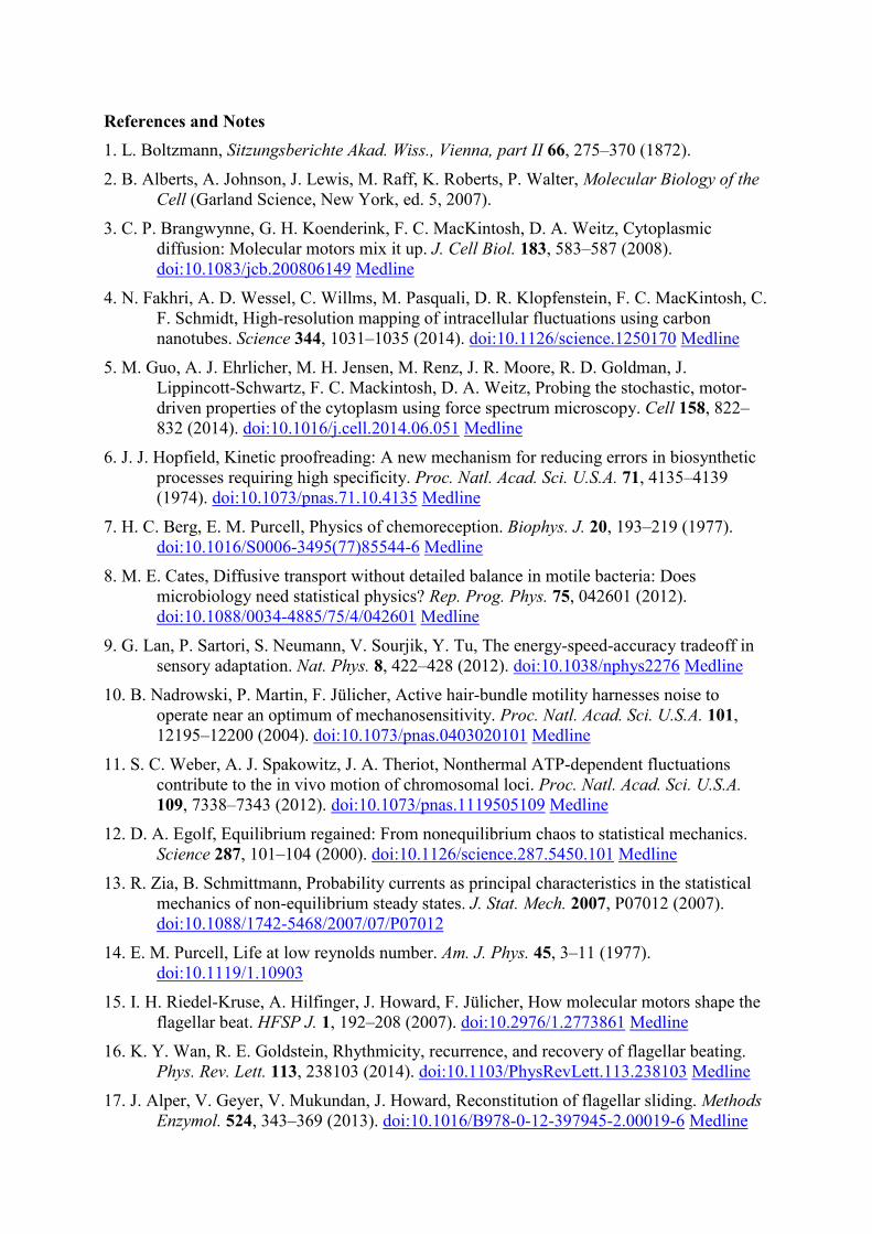
4.4Analysisofmicrotubulefluctuations:Asanegativecontrolofourmethodwhenappliedtoan equilibrium system,we tracked the transverse thermal bending fluctuations of an 85 µmlongmicrotubuleover5.5minutes.FigureS18AandBshowtimetracesofthefirsttwobendingmodes,whileFig. S18Cdepicts the resultsofPFAon these trajectories.As in thecaseof theATP-depleted and blebbistatin-treated cilia, themajority of arrows havemagnitudes smallerthan the radius of their error discs, indicating a lack of significant currents. Additionally, wetestedwhetherthenoisyclockwisecurrentenclosedbythedashedwhiteboxwassignificantbybootstrapping its contour integral aspreviouslydescribed. The resultinghistogram, shown inFig. S17D, is centered at 0.64, indicating amarginal (p = 0.26) significance of the circulationpattern.

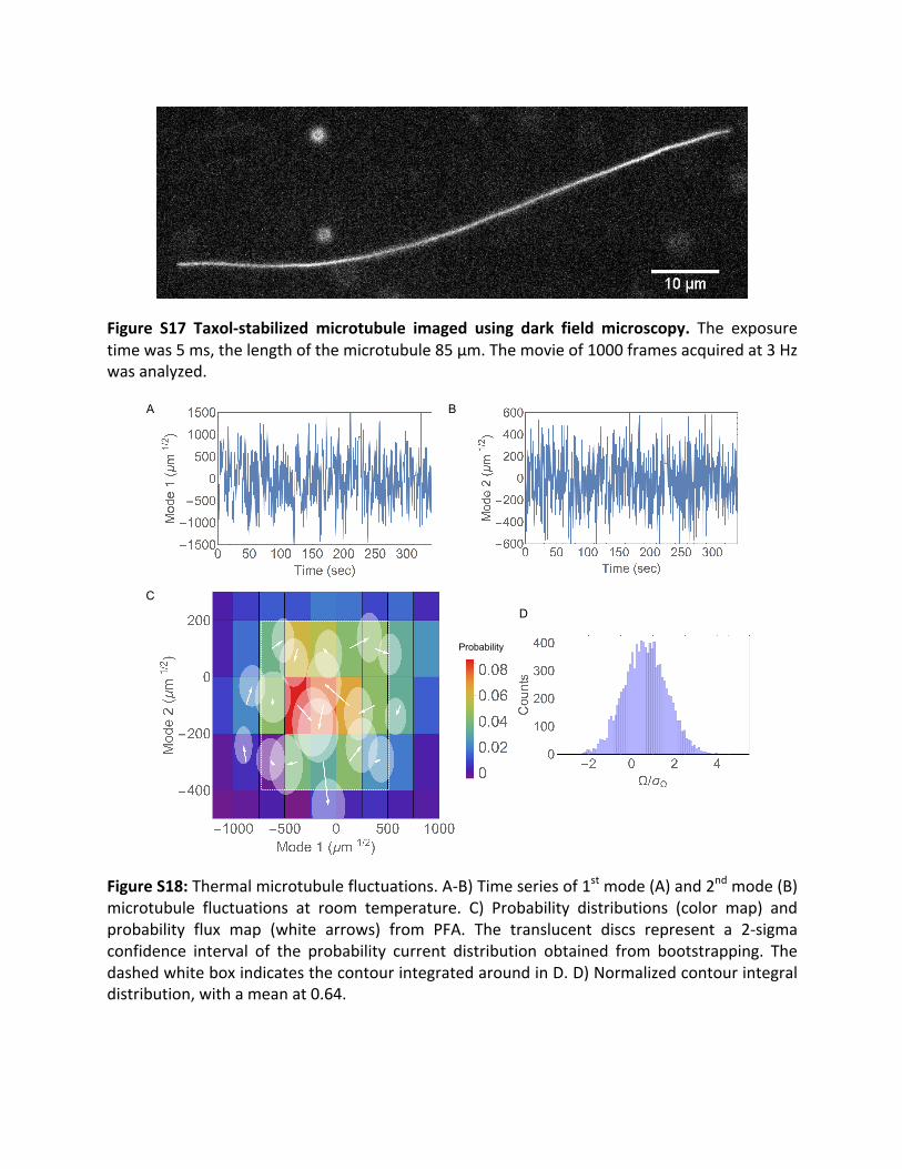
Figure S17 Taxol-stabilized microtubule imaged using dark field microscopy. The exposuretimewas5ms,thelengthofthemicrotubule85µm.Themovieof1000framesacquiredat3Hzwasanalyzed.

FigureS18:Thermalmicrotubulefluctuations.A-B)Timeseriesof1stmode(A)and2ndmode(B)microtubule fluctuations at room temperature. C) Probability distributions (color map) andprobability flux map (white arrows) from PFA. The translucent discs represent a 2-sigmaconfidence interval of the probability current distribution obtained from bootstrapping. ThedashedwhiteboxindicatesthecontourintegratedaroundinD.D)Normalizedcontourintegraldistribution,withameanat0.64.

BA

CD

Probability

References and Notes 1. L. Boltzmann, Sitzungsberichte Akad. Wiss., Vienna, part II 66, 275–370 (1872).

2. B. Alberts, A. Johnson, J. Lewis, M. Raff, K. Roberts, P. Walter, Molecular Biology of theCell (Garland Science, New York, ed. 5, 2007).

3. C. P. Brangwynne, G. H. Koenderink, F. C. MacKintosh, D. A. Weitz, Cytoplasmicdiffusion: Molecular motors mix it up. J. Cell Biol. 183, 583–587 (2008). doi:10.1083/jcb.200806149 Medline

4. N. Fakhri, A. D. Wessel, C. Willms, M. Pasquali, D. R. Klopfenstein, F. C. MacKintosh, C.F. Schmidt, High-resolution mapping of intracellular fluctuations using carbon nanotubes. Science 344, 1031–1035 (2014). doi:10.1126/science.1250170 Medline

5. M. Guo, A. J. Ehrlicher, M. H. Jensen, M. Renz, J. R. Moore, R. D. Goldman, J.Lippincott-Schwartz, F. C. Mackintosh, D. A. Weitz, Probing the stochastic, motor-driven properties of the cytoplasm using force spectrum microscopy. Cell 158, 822–832 (2014). doi:10.1016/j.cell.2014.06.051 Medline

6. J. J. Hopfield, Kinetic proofreading: A new mechanism for reducing errors in biosyntheticprocesses requiring high specificity. Proc. Natl. Acad. Sci. U.S.A. 71, 4135–4139 (1974). doi:10.1073/pnas.71.10.4135 Medline

7. H. C. Berg, E. M. Purcell, Physics of chemoreception. Biophys. J. 20, 193–219 (1977).doi:10.1016/S0006-3495(77)85544-6 Medline

8. M. E. Cates, Diffusive transport without detailed balance in motile bacteria: Doesmicrobiology need statistical physics? Rep. Prog. Phys. 75, 042601 (2012). doi:10.1088/0034-4885/75/4/042601 Medline

9. G. Lan, P. Sartori, S. Neumann, V. Sourjik, Y. Tu, The energy-speed-accuracy tradeoff insensory adaptation. Nat. Phys. 8, 422–428 (2012). doi:10.1038/nphys2276 Medline

10. B. Nadrowski, P. Martin, F. Jülicher, Active hair-bundle motility harnesses noise tooperate near an optimum of mechanosensitivity. Proc. Natl. Acad. Sci. U.S.A. 101, 12195–12200 (2004). doi:10.1073/pnas.0403020101 Medline

11. S. C. Weber, A. J. Spakowitz, J. A. Theriot, Nonthermal ATP-dependent fluctuationscontribute to the in vivo motion of chromosomal loci. Proc. Natl. Acad. Sci. U.S.A. 109, 7338–7343 (2012). doi:10.1073/pnas.1119505109 Medline

12. D. A. Egolf, Equilibrium regained: From nonequilibrium chaos to statistical mechanics.Science 287, 101–104 (2000). doi:10.1126/science.287.5450.101 Medline

13. R. Zia, B. Schmittmann, Probability currents as principal characteristics in the statisticalmechanics of non-equilibrium steady states. J. Stat. Mech. 2007, P07012 (2007). doi:10.1088/1742-5468/2007/07/P07012

14. E. M. Purcell, Life at low reynolds number. Am. J. Phys. 45, 3–11 (1977).doi:10.1119/1.10903

15. I. H. Riedel-Kruse, A. Hilfinger, J. Howard, F. Jülicher, How molecular motors shape theflagellar beat. HFSP J. 1, 192–208 (2007). doi:10.2976/1.2773861 Medline

16. K. Y. Wan, R. E. Goldstein, Rhythmicity, recurrence, and recovery of flagellar beating.Phys. Rev. Lett. 113, 238103 (2014). doi:10.1103/PhysRevLett.113.238103 Medline

17. J. Alper, V. Geyer, V. Mukundan, J. Howard, Reconstitution of flagellar sliding. MethodsEnzymol. 524, 343–369 (2013). doi:10.1016/B978-0-12-397945-2.00019-6 Medline

18. Materials and methods are available as supplementary materials on Science Online.

19. S. R. Aragon, R. Pecora, Dynamics of wormlike chains. Macromolecules 18, 1868–1875 (1985). doi:10.1021/ma00152a014

20. R. Ma, G. S. Klindt, I. H. Riedel-Kruse, F. Jülicher, B. M. Friedrich, Active phase and amplitude fluctuations of flagellar beating. Phys. Rev. Lett. 113, 048101 (2014). doi:10.1103/PhysRevLett.113.048101 Medline

21. R. P. Feynman, R. B. Leighton, M. Sands, The Feynman Lectures on Physics, vol 1. (Addison-Wesley, Reading, MA, 1966).

22. K. Sekimoto, Kinetic characterization of heat bath and the energetics of thermal ratchet models. J. Phys. Soc. Jpn. 66, 1234–1237 (1997). doi:10.1143/JPSJ.66.1234

23. C. E. Shannon, W. Weaver, The Mathematical Theory of Communication (Univ. of Illinois Press, Urbana, 1949).

24. V. Singla, J. F. Reiter, The primary cilium as the cell’s antenna: Signaling at a sensory organelle. Science 313, 629–633 (2006). doi:10.1126/science.1124534 Medline

25. C. Battle, C. M. Ott, D. T. Burnette, J. Lippincott-Schwartz, C. F. Schmidt, Intracellular and extracellular forces drive primary cilia movement. Proc. Natl. Acad. Sci. U.S.A. 112, 1410–1415 (2015). doi:10.1073/pnas.1421845112 Medline

26. B. G. Barnes, Ciliated secretory cells in the pars distalis of the mouse hypophysis. J. Ultrastruct. Res. 5, 453–467 (1961). doi:10.1016/S0022-5320(61)80019-1 Medline

27. D. Mizuno, C. Tardin, C. F. Schmidt, F. C. Mackintosh, Nonequilibrium mechanics of active cytoskeletal networks. Science 315, 370–373 (2007). doi:10.1126/science.1134404 Medline

28. C. P. Brangwynne, G. H. Koenderink, F. C. Mackintosh, D. A. Weitz, Nonequilibrium microtubule fluctuations in a model cytoskeleton. Phys. Rev. Lett. 100, 118104 (2008). doi:10.1103/PhysRevLett.100.118104 Medline

29. I. Antoniades, P. Stylianou, P. A. Skourides, Making the connection: Ciliary adhesion complexes anchor basal bodies to the actin cytoskeleton. Dev. Cell 28, 70–80 (2014). doi:10.1016/j.devcel.2013.12.003 Medline

30. W. F. Marshall, Basal bodies: Platforms for building cilia. Curr. Top. Dev. Biol. 85, 1–22 (2008). doi:10.1016/S0070-2153(08)00801-6 Medline

31. J. Prost, J. F. Joanny, J. M. Parrondo, Generalized fluctuation-dissipation theorem for steady-state systems. Phys. Rev. Lett. 103, 090601 (2009). doi:10.1103/PhysRevLett.103.090601 Medline

32. C. Bustamante, J. Liphardt, F. Ritort, The nonequilibrium thermodynamics of small systems. Phys. Today 58, 43–48 (2005). doi:10.1063/1.2012462

33. G. E. Crooks, Entropy production fluctuation theorem and the nonequilibrium work relation for free energy differences. Phys. Rev. E Stat. Phys. Plasmas Fluids Relat. Interdiscip. Topics 60, 2721–2726 (1999). doi:10.1103/PhysRevE.60.2721 Medline

34. C. Jarzynski, Nonequilibrium equality for free energy differences. Phys. Rev. Lett. 78, 2690–2693 (1997). doi:10.1103/PhysRevLett.78.2690

35. J. Liphardt, S. Dumont, S. B. Smith, I. Tinoco Jr., C. Bustamante, Equilibrium information from nonequilibrium measurements in an experimental test of Jarzynski’s equality. Science 296, 1832–1835 (2002). doi:10.1126/science.1071152 Medline

36. U. Seifert, Entropy production along a stochastic trajectory and an integral fluctuation theorem. Phys. Rev. Lett. 95, 040602 (2005). doi:10.1103/PhysRevLett.95.040602 Medline

37. R. Ma, G. S. Klindt, I. H. Riedel-Kruse, F. Jülicher, B. M. Friedrich, Active phase and amplitude fluctuations of flagellar beating. Phys. Rev. Lett. 113, 048101 (2014). doi:10.1103/PhysRevLett.113.048101 Medline

38. K. Y. Wan, R. E. Goldstein, Rhythmicity, recurrence, and recovery of flagellar beating. Phys. Rev. Lett. 113, 238103 (2014). doi:10.1103/PhysRevLett.113.238103 Medline

39. E. M. Purcell, Life at low reynolds number. Am. J. Phys. 45, 3–11 (1977). doi:10.1119/1.10903

40. H. Sillescu, R. Bohmer, G. Diezemann, G. Hinze, Heterogeneity at the glass transition: What do we know? J. Non-crystalline Solids 307-310, 16–23 (2002). doi:10.1016/S0022-3093(02)01435-7

41. K. Kim, S. Saito, Multi-time density correlation functions in glass-forming liquids: Probing dynamical heterogeneity and its lifetime. J. Chem. Phys. 133, 044511 (2010). doi:10.1063/1.3464331 Medline

42. C. P. Brangwynne, G. H. Koenderink, F. C. Mackintosh, D. A. Weitz, Nonequilibrium microtubule fluctuations in a model cytoskeleton. Phys. Rev. Lett. 100, 118104 (2008). doi:10.1103/PhysRevLett.100.118104 Medline

43. P. Bursac, G. Lenormand, B. Fabry, M. Oliver, D. A. Weitz, V. Viasnoff, J. P. Butler, J. J. Fredberg, Cytoskeletal remodelling and slow dynamics in the living cell. Nat. Mater. 4, 557–561 (2005). doi:10.1038/nmat1404 Medline

44. G. Massiera, K. M. Van Citters, P. L. Biancaniello, J. C. Crocker, Mechanics of single cells: Rheology, time dependence, and fluctuations. Biophys. J. 93, 3703–3713 (2007). doi:10.1529/biophysj.107.111641 Medline

45. J. Alper, V. Geyer, V. Mukundan, J. Howard, Reconstitution of flagellar sliding. Methods Enzymol. 524, 343–369 (2013). doi:10.1016/B978-0-12-397945-2.00019-6 Medline

46. C. Leduc, F. Ruhnow, J. Howard, S. Diez, Detection of fractional steps in cargo movement by the collective operation of kinesin-1 motors. Proc. Natl. Acad. Sci. U.S.A. 104, 10847–10852 (2007). doi:10.1073/pnas.0701864104 Medline

47. F. Ruhnow, D. Zwicker, S. Diez, Tracking single particles and elongated filaments with nanometer precision. Biophys. J. 100, 2820–2828 (2011). doi:10.1016/j.bpj.2011.04.023 Medline

48. S. R. Aragon, R. Pecora, Dynamics of wormlike chains. Macromolecules 18, 1868–1875 (1985). doi:10.1021/ma00152a014

49. C. Battle, C. M. Ott, D. T. Burnette, J. Lippincott-Schwartz, C. F. Schmidt, Intracellular and extracellular forces drive primary cilia movement. Proc. Natl. Acad. Sci. U.S.A. 112, 1410–1415 (2015). doi:10.1073/pnas.1421845112 Medline

50. C. Battle, L. Lautscham, C. F. Schmidt, Differential interference contrast microscopy using light-emitting diode illumination in conjunction with dual optical traps. Rev. Sci. Instrum. 84, 053703 (2013). doi:10.1063/1.4804597 Medline

51. G. Danuser, P. T. Tran, E. D. Salmon, Tracking differential interference contrast diffraction line images with nanometre sensitivity. J. Microsc. 198, 34–53 (2000). doi:10.1046/j.1365-2818.2000.00678.x Medline

52. D. Sage, F. R. Neumann, F. Hediger, S. M. Gasser, M. Unser, Automatic tracking of individual fluorescence particles: Application to the study of chromosome dynamics. IEEE Trans. Image Process. 14, 1372–1383 (2005). doi:10.1109/TIP.2005.852787 Medline

53. E. A. Schwartz, M. L. Leonard, R. Bizios, S. S. Bowser, Analysis and modeling of the primary cilium bending response to fluid shear. Am. J. Physiol. 272, F132–F138 (1997). Medline

54. Y. N. Young, M. Downs, C. R. Jacobs, Dynamics of the primary cilium in shear flow. Biophys. J. 103, 629–639 (2012). doi:10.1016/j.bpj.2012.07.009 Medline