Surface tension in incompressible Rayleigh–Taylor mixing flowyyoung/young_papers/Young2006.pdf · The Rayleigh–Taylor (RT) instability is a fingering instability of fluid interface

Journal of TurbulenceVolume 7, No. 71, 2006

Surface tension in incompressible Rayleigh–Taylormixing flow

Y.-N. YOUNG∗† and F. E. HAM‡

†Department of Mathematical Sciences, New Jersey Institute of Technology, Newark, NJ 07102, USA‡Department of Mechanical Engineering, Stanford University, Stanford, CA 94305, USA

We study the effect of surface tension on the incompressible Rayleigh–Taylor instability. We modifyGoncharov’s local analysis [1] to consider the surface tension effect on the Rayleigh–Taylor bubblevelocity. The surface tension damps the linear instability and reduces the nonlinear terminal bubblevelocity. We summarize the development of a finite-volume, particle-level-set, two-phase flow solverwith an adaptive Cartesian mesh, and results from convergence and validation studies of this two-phase flow solver are provided. We use this code to simulate the single-mode, viscous Rayleigh–Taylor instability with surface tension, and good agreement in terminal bubble velocity is found whencompared with analytic results. We also simulate the immiscible Rayleigh–Taylor instability withrandom initial perturbations. The ensuing mixing flow is characterized by the effective mixing rateand the flow anisotropy. Surface tension tends to reduce the effective mixing rate and homogenizesthe Rayleigh–Taylor mixing flow. Finally, we provide a scaling argument for detecting the onset ofthe quadratic, self-similar Rayleigh–Taylor growth.

Keywords: Rayleigh–Taylor instability; Surface tension; Anisotropy; Transition; Self-similar turbulence

PACS numbers: 52.35.Py; 47.11.Df; 68.03.−g; 68.03.Cd; 47.52.+j; 47.11.−j; 47.35.−i; 47.27.−i; 47.51.+a; 47.27.wj

1. Introduction

The Rayleigh–Taylor (RT) instability is a fingering instability of fluid interface when lightfluid is accelerated against the heavy fluid. A principle focus of study on the Rayleigh–Taylorinstability is the global mixing rate as the instability evolves and develops into turbulence.Recent simulations on miscible Rayleigh–Taylor instability show that the RT mixing ratedepends sensitively on initial conditions [2–4]. Many other factors may influence the RTmixing, such as (numerical) mass diffusion [5, 6], surface tension [7], viscosity, compressibility[8], time dependence of driving acceleration, shocks, geometric effects and varied forms ofheterogeneity.

Significant progress has accumulated from experiments, direct numerical simulations andanalysis on the miscible RT mixing in the Boussinesq limit, where the density contrast isalmost zero (the Atwood number A ≡ ρh−ρl

ρh+ρl → 0) and the buoyancy Ag is finite (g is theacceleration). Experiments and simulations show that mass diffusion can reduce the RT mixingrate by as much as a half [9–12]. Analysis on the Boussinesq RT turbulence illustrates that theself-similar RT turbulence can be completely determined by the conditions at the onset of the

∗Corresponding author. E-mail: [email protected]

Journal of TurbulenceISSN: 1468-5248 (online only) c© 2006 Taylor & Francis

http://www.tandf.co.uk/journalsDOI: 10.1080/14685240600809979

2 Y.-N. Young and F. E. Ham

self-similar process [13], where the mixing zone width (or amplitude) h grows quadraticallywith time (h = αgAt2). This finding is consistent with the sensitive dependence of the mixingrate α on initial perturbations [2, 4, 14], as different initial conditions may lead to different flowsat the onset of the self-similar RT growth. Once the self-similar growth is initiated, the energycontaining scale increases (l ∼ Agt2) whereas the Kolmogorov scale decreases with time(η ∼ (A2g2/ν3)−1/4t−1/4). As time progresses, the inertial range becomes large enough forestablishing the forward cascade in the energy spectrum, and turbulence will be fully developedin the RT mixing zone. For this miscible RT turbulence, the scaling and turbulent mixing aredescribed by the phenomenological model [15]. Thus, from the initial growth of the instabilityto the asymptotic turbulent state, the evolution of Boussinesq miscible RT mixing can becompletely characterized by the flow conditions at the transition to self-similar growth, whichis estimated to occur at t ∼ 15tc = 15(ν/g2A2)1/3 [13]. It is unclear if the above Boussinesqresults may be directly applied to the immiscible RT mixing with finite Atwood numbers.

Motivated by these studies on Boussinesq RT mixing, in this paper we focus on character-izing the immiscible RT instability by identifying the transition to the nonlinear evolution andthe transition to the self-similar growth. In particular, we will focus on the effects of surfacetension and finite Atwood number on transitions between different evolutionary stages.

For single-mode RT instability withA = 1, the transition from linear to nonlinear dynamicsoccurs when the mode amplitude hk ∼ 1/k [16], where k is the wavenumber. As the amplitudeincreases, the rising bubble will reach a constant terminal velocity. Goncharov [1] extendedpotential flow models in Layzer [17] and Hecht et al. [18] to an arbitrary Atwood number. Hefound the terminal bubble velocity vb to be a function of A:

vb =√

2A1 + A

g

Ck, (1)

where C = 3 (1) for two (three)-dimensional geometries. Recent results from simulations ofsingle-mode RT instability show that Goncharov’s model gives better agreement than otherpotential flow models (see [19] and references therein) and vortex sheet simulations by Sohn[20]. We will modify the local potential flow analysis in [1] to consider the surface tensioneffect on the single-mode Rayleigh–Taylor instability. Results from this analysis show thatthe terminal bubble velocity is reduced by surface tension. We will also compare the analyticprediction with direct simulation of single-mode, immiscible RT instability in section 3.

For a broadband of unstable modes, a quadratic, self-similar growth ensues after nonlinearitytakes over the initial exponential growth of the RT instability. Dimonte [14] summarized howunstable modes grow and evolve to give rise to the self-similar RT turbulence. Assuming thateach mode reaches a terminal velocity, independent of the other growing modes, the self-similar expansion is envisioned to be the result of a succession of dominant bubbles fromsmall sizes at small amplitudes to large bubbles at large amplitudes. From this model, theself-similar quadratic growth is possible if the initial perturbation amplitudes vary inverselywith the wavenumber hk ∼ 1/k2. For the Boussinesq RT turbulence, a self-similar analysis

[13] on the averaged moment equations shows that the mixing rate α = C04 (1 +

√4h0

AgC0t2 ),where C2

0 is the variance of the density fluctuation at the center of the mixing zone. Theself-similar solution requires C0 to be a constant that is determined by the density variance atthe onset of the self-similar turbulence. The onset of the self-similar growth is estimated tooccur at t = 15tc, when the diffusive regime ends. Such an estimate may not be reasonablefor the immiscible RT instability, where there is no molecular mass diffusion. Refining theself-similar analysis in [13], we present a scaling argument that allows us to detect the onsetof the self-similar growth without referring to the diffusion regime. With this we can estimatethe transition to self-similar growth for immiscible RT mixing with large density contrast.

Surface tension in incompressible Rayleigh–Taylor mixing flow 3

This paper is organized as follows. In section 2 we present the local potential flow analysisfor single-mode RT instability. In section 3 we summarize the problem formulation of theviscous, immiscible RT instability and the numerics of the finite-volume, particle-level-set(FV-PLS) flow solver. We also provide detailed code validation and convergence results. Insection 4 we present results of direct simulations of immiscible RT mixing for various valuesof surface tension and density contrast. Finally, in section 5 we propose a scaling argumentfor detecting the onset of the self-similar RT growth in general situations, and we also providesome future directions.

2. Surface tension effect on single-mode RT instability

In this section we consider the effect of surface tension on the RT instability of an inviscid(ν = 0) potential flow. These analytic results will be used to validate the incompressibletwo-phase flow solver summarised in the next section.

In the analysis we assume the surface tension to be small enough for the instability to growand form a bubble/spike configuration. The fluids are subject to an external acceleration galong the y axis, pushing the heavy fluid toward the light fluid. The fluid interface is locatedat y = η(x, t), and the velocity potential φ obeys the Laplace equation

∇2φ = (∂2

x + ∂2y

)φ = 0. (2)

The governing equations for two irrotational, incompressible, inviscid fluids in two dimensionsare

∂tη + uh∂xη = vh, (3)

[v − u∂xη] = 0, (4)[ρ

(∂tφ + 1

2u2 + gη

)]+ [P] = 0, (5)

with velocity u = (u, v) = ∇φ and P is the pressure. [Q] ≡ Qh − Ql , where the superscriptsh and l denote the heavy- and light-fluid variables, respectively. The pressure jump in equation(5) is equal to the surface tension force

[P] = Ph − Pl = −σκ, (6)

where σ is the surface tension coefficient and κ is the local curvature. We expand the bubbleshape η in x near the bubble tip:

η = η0(t) + η2(t)x2 + O(x3), (7)

with |x | � 1 and η2 is related to the bubble radius R as R = −1/(2η2). Following Goncharov’sapproach, we adopt the following velocity potentials at the bubble tip:

φh = a1(t) cos(kx)e−k(y−η0), (8)

φl = b1(t) cos(kx)ek(y−η0) + b2(t)y, (9)

where a1, b1 and b2 are amplitudes to be determined. For the parabolic bubble profile inequation (7), the bubble curvature κ is approximated as

κ ∼ −2η2

3

√1 + 4η2

2x2∼ −2η2

(1 − 6η2

2x2). (10)


Substituting equations (8)–(9) into equation (5) and expanding in x around the bubble tip, weobtain the following equations at the zeroth order in x :

η2 = −η0k2 (k + 6η2), (11)

ρh

(a1 + 1

2 k2a21 + gη0

)− ρl

(b1 + b2η0 + 1

2 k2b21 + kb1b2 + 1

2 b22 + gη0

)+ 2η2σ = 0.

(12)

a1, b1 and b2 can be expressed in terms of η0 and η2 after we substitute φh and φl into equations(3)–(4):

a1 = − η0

k, b1 = η0(k + 6η2)

k(k − 6η2), b2 = 12η0η2

6η2 − k. (13)

Substituting the above expressions into equation (12) and linearizing with respect to the basestate of a flat interface, we find the following linear equation for η0:

ρh

(− η0

k+ gη0

)− ρl

(η0

k+ gη0

)− k2ση0 = 0 . (14)

Assuming the form of normal mode for η0 (η0 = entη′0), we find the linear growth rate

n =√Agk − k3σ

ρh + ρl, (15)

which is identical to the linear analysis results for inviscid RT instability with surface tension[21]. At the quadratic order in x , the evolution equation for amplitude η0 is obtained:

η0k2 − 4Akη2 − 12Aη2

2

2(k − 6η2)+ η2

0k2 (4A − 3)k2 + 6(3A − 5)kη2 + 36Aη22

2(k − 6η2)2

+Agη2 − 12ση32

ρh + ρl= 0. (16)

Similar to Goncharov’s analysis without surface tension, we find that, in the limit t → ∞, thebubble curvature η2 and the bubble velocity η0 approach their asymptotic values

η2(t → ∞) = −k

6, η0(t → ∞) =

√2A

1 + Ag

3k− σk

9ρh. (17)

For axi-symmetric RT bubbles, we obtain the following bubble curvature and terminal velocity:

η2(t → ∞) = −k

8, η0(t → ∞) =

√2A

1 + Ag

k− 3σk

16ρh. (18)

It can be shown that the steady states in equations (17)–(18) are linearly stable to smallperturbations.

In deriving equations (17)–(18) for the terminal bubble velocity, we have assumed aparabolic bubble shape with a curvature −2η2. Therefore, the instability has to grow firstfor the analysis to be valid, and the condition

σ ≤ σc ≡ g(ρh − ρl)

k2(19)

must be satisfied for equations (17)–(18) and the above analysis with the surface tension tohold. From this condition, we obtain a lower bound on the bubble terminal velocity for a given


wavenumber and Atwood number

vb >

√C

2A1 + A

g

k, (20)

where C = 29 in two dimensions and C = 13

16 in three dimensions.In the next section we use results from the above analysis (equations (17)–(18)) to validate

the FV-PLS two-phase flow solver. As will be illustrated, we obtain reasonable agreementbetween the analytic and the numerical results for small fluid viscosity (ν = 10−3) in thedirect simulations of single-mode immiscible RT instability.

3. Formulation, numerics and validation

We first formulate the two-fluid system in the level-set framework. We then briefly summarizethe essential numerics developed for the Cartesian adaptive grid. The key numerical develop-ment is the treatment of immersed, continuum surface tension force in the finite-volume fluidsolver on the (homogeneously adaptive) Cartesian grid. We then present validation of usingthis two-phase solver to simulate the viscous, immiscible RT instability and mixing.

3.1 Formulation and numerics

The incompressible, immiscible, viscous two-fluid system is formulated as a one-fluid systemwith variations of density and viscosity only in the neighborhood of the interface. The fluidinterface is described by a level-set function φ(x, t) = 0. With constant density and viscosityin each phase (fluid), the total density and viscosity can be written as

ρ = ρ(φ) = ρh H (φ) + ρl(1 − H (φ)), µ = µ(φ) = µh H (φ) + µl(1 − H (φ)), (21)

where ρh,l and µh,l are constant density and viscosity of the heavy or light fluid, respectively,and H (φ) is the Heaviside function: H (φ) = 1 if φ > 0 and H (φ) = 0 if φ < 0. Formulatedas such, the continuity equation can be decomposed into the the following equations:

∂φ

∂t+ u · ∇φ = 0

∣∣∣∣φ=0

, ∇ · u = 0, (22)

where u is the fluid velocity. Our numerical flow solver deals with the collocated velocities asthe primitive variables; thus, the Navier–Stokes equations take the following form:

ρ∂u∂t

+ ρ∇(uu) = −∇ p + ∇(µ∇u) − ρgk + σκδ(d)n, (23)

where p is the pressure, g is the gravitational acceleration, σ is the surface tension coefficient,κ is the local surface curvature, δ(d) is the delta function based on the normal distance d tothe surface and n is the outward unit normal vector at the free surface. Equations (21)–(23)comprise the governing equations for the two-fluid system. It is important that we choose anaccurate and efficient numerical scheme for evolving the level set to mitigate the numericalerror in conserving mass and momentum. We solve equations (22)–(23) on a Cartesian adaptivegrid. The grid arrangement and adaptation are described in [22], and here we only discussdetails pertaining to the simulation of the two-phase flow.

All variables are stored at the control volume (CV) centers (with the exception of a face-normal velocity located at the face centers) and are used to enforce the divergence-free con-straint at each time step. The variables are staggered in time for convenience in the time


advancement scheme; the velocities are located at time levels tn and tn+1; and pressure, den-sity, viscosity and the level set at time levels tn−1/2 and tn+1/2. The semi-discretization of thegoverning equations at each time step is then as follows.

Step 1. Advance and reinitialize the level set

φn+1/2 − φn−1/2

t+ un

j

1

2

∂

∂x j(φn−1/2 + φn+1/2) = 0. (24)

The spatial derivatives in the level-set equation (equation (24)) are approximated by afifth-order WENO scheme [23]. Uniform, homogeneous grid refinement is enforced within aband around the zero level-set. For updating the level-set function, we use an implicit Crank–Nicholson scheme which requires an iterative method. In practice, the hyperbolic system is notstiff and can be quickly converged by a simple iterative scheme such as the Gauss–Seidel itera-tion. We note that in the present time-staggering scheme, equation (24) is decoupled from otherequations and is advanced based on un to the next time level. The following reinitializationstep is performed every step to ensure that the level set is a signed distance function

∂φ

∂τ= sgn(φ)(1 − |∇φ|). (25)

The spatial derivatives in reinitialization are once again approximated using the fifth-orderWENO scheme. We use an explicit third-order TVD Runge–Kutta method for timeintegration. In practice, five iterations with a pseudo-time step of τ = x/4 are sufficient.

In addition, we have utilized particles to improve the level set. Markers help minimize themovement of the level set during the reinitialization step, and reduce unnecessary mergingof the level set due to numerical discretization/diffusion. This formulation is based on thehybrid-particle-level-set method [24]. Recent results show that the particle-level-set methodis accurate and comparable to the most accurate front-tracking schemes. In standard tests suchas the Zalesek disk and the time-reversal vortex flow, the particle-level-set method outperformsthe usual level-set methods by reducing numerical diffusion [24, 25] in the level-set framework.

Step 2. Update the density and viscosity at tn+1/2. With the level set advanced, fluid propertiesare calculated based on the level set at the mid-point of the time interval:

ρn+1/2 = ρh H (φn+1/2) + ρl(1 − H (φn+1/2)),

µn+1/2 = µh H (φn+1/2) + µl(1 − H (φn+1/2)). (26)

In the present investigation, we use a smoothed property variation in the region of the zerolevel set as described by Sussman et al. [26]. This smoothed variation leads to a surface tensionforce that is of the C2 class in the categorization for the immersed (continuous) delta function[27].

Step 3. Update the incompressible velocities at tn+1. The procedures used to update theincompressible velocities are a variant of the collocated fractional step method [28]. We payspecial attention to the discrete form of force terms that have rapid spatial variation aroundthe interface, such as the surface tension forces in the momentum equation. First, a projectedvelocity field ui is calculated:

ui − uni

t= − 1

ρn+1/2

(∂p

∂xi

n−1/2

+ Rn+1/2i

), (27)

where Ri contains all other terms in the momentum equation. We discretize both the convectiveand viscous terms implicitly using second-order symmetric discretizations. The surface tension


is treated explicitly based on φn+1/2 (the level set at the midpoint of the current time step).We then subtract the old pressure gradient and interpolate the velocity field to the faces. In theinterpolation step, a critical difference between our formulation and the formulation of Kimand Choi [28] is in the calculation of the face-normal velocities. Kim and Choi assume

Rin+1/2

ρn+1/2

f

≈ Rn+1/2f

ρn+1/2f

, (28)

where ()f

is a second-order interpolation operator that yields a face-normal component fromtwo CV-centered vectors. This is an O(x2) approximation, seemingly consistent with theoverall accuracy of the method, and significantly simplifies the calculation of the Poissonequation source term. However, when surface tension forces are introduced we find that thisapproximation can lead to large non-physical oscillations in the CV-centered velocity field. Tosolve this problem, the surface tension forces must be calculated at the faces and then averagedto the CV centers, i.e.

Rσi

ρ≡ Rσ

f

ρ f

xi

. (29)

With this calculation of the surface tension force, we have to include the additional terms inthe calculation of the source term in the Poisson equation for the pressure.

3.2 Code validation

First, we illustrate the importance of a proper handling of the surface tension force. Figure 1(a)compares the calculated pressure along the horizontal center line: the dashed line is from us-ing Kim and Choi’s formulation for the surface tension force, and the solid line is from usingequation (29). Clearly, our formulation results in a better pressure with a small amplitudeof the velocity field (figure 1(b)) that should be exactly zero. These ‘parasitic currents’ havebeen reported by other investigators ([29], for example), and in our formulation the maxi-mum parasitic velocity is on the order of 0.001σ/µ for an equivalent uniform grid spacingx = 1

64 and the Ohnesorge number Oh ≡ (µ2/aρσ )0.5 = 2.1. This is consistent with theobservations of others using staggered structured codes. Figure 1(c) shows a comparison be-tween the linear analysis results and the computed periodicity of capillary wave on a sphericaldrop, with generally good agreement, and the error in the capillary frequency is less than1%.

Next, we present validation of using the FV-PLS two-phase flow solver to simulate theRayleigh–Taylor instability. For these convergence tests, the computation domain size is 1 ×1 × 8, and the originally flat interface is placed at z = 4. Periodic boundary conditions areadopted in the horizontal directions, and wall boundary conditions are used in the gravitationaldirection. We perturb the interface with a sinusoidal perturbation a0(cos(kx) + cos(ky)), wherethe wavenumber k = 2π and the amplitude a0 = 0.01. The grid spacing for the velocity awayfrom the interface is fixed at x f = 0.2, and we vary the minimum grid spacing around theinterface xs from 0.2 to 0.025.

The results in figure 2(a) are for the Atwood number A = 0.1 and the kinetic viscosityνh = νl = 10−3. As shown in figure 2(a), the bubble height (hb) converges as we decrease xs .Similar convergence is also found for the down-welling spikes in these A = 0.1 simulations.For the Atwood number A ∼ 1, the spikes of the heavy fluid are (almost) free-falling into thelight fluid [30], whereas the bubbles of the light fluid reach a terminal velocity [1]. Due tosuch asymmetry between bubble and spike, more resolution is necessary to resolve the pointy


Figure 1. (a) A comparison of pressure for two different formulations of the surface tension force. The dashedline is from Kim and Choi’s formulation and the solid line is from our formulation of the surface tension force.(b) Parasitic currents around a circular drop. The amplitude of the parasitic flow is ∼0.001σ/µ. (c) A comparisonbetween computed and theoretical oscillation periods for a spherical drop.

spikes at large A. Figure 2(b) shows the convergence of spike depth hs as we decrease xs

from 0.2 to 0.0125. In figure 2(c) we show the order of convergence for results in panels(a) and (b). The second-order convergence for spikes with A = 0.9 (solid line) is due to thefact that the error in the velocity field around the spike dominates the error in capturing theinterface; thus, the order of convergence is that of the flow solver, which is of the second order[22]. However, for bubbles with A = 0.1 (dashed line) the numerical error is dominated bythat in capturing the interface; thus it is slightly larger than order 1.

Figure 3(a) demonstrates that, for a single-mode perturbation with k = 2π , σ = 0 and fluidviscosity νh = νl = 10−3, the code reproduces the growth rate from linear analysis for Atwoodnumbers from 0.1 to 0.9 [21]. The sinusoidal perturbation grows exponentially and eventuallysaturates. During the nonlinear evolution, the bubble reaches a terminal velocity as shownin figure 3(b), where we plot the bubble velocity (scaled by equation (1)) versus the bubbleheight hb. In figure 3(c) we plot the terminal bubble velocity from our simulations using twominimum grid spacings x f . The solid line is the terminal bubble velocity from equation


Time

A=0.1

0.025

0.2

0.1

0.05(dashed line)

(solid line)

Bubb

le H

eight

hb

Spik

e Dep

th h

s

L1−n

orm

Err

or in

h

(a)

0.025

0.05(dashed line)

(solid line)

Time

0.1

0.2

A=0.9(b)

Minimum Grid Spacing around the interface

Bubble height for A=0.1

Spike Depth for A=0.9

(c)

Figure 2. (a) Convergence test for bubble height for A = 0.1. (b) Convergence test for spike depth for A = 0.9.(c) L1-error versus xs . The squares are for spike depth with A = 0.9 and the diamonds are for bubble height withA = 0.1. The solid line is proportional to (xs )2 and the dashed line is proportional to (xs )1.2.

(1). A comparison between numerical simulations of single-mode RT instability with several(inviscid) potential flow models shows that Goncharov’s model gives the best agreement withsimulation results for all values of the Atwood number [19]. In addition, the largest deviationbetween simulation results and Goncharov’s model is found for the Atwood number A ∼ 0.6[19], similar to our results in figure 3(c).

For small Atwood numbers in figure 3(b), the bubble velocity overshoots and decreasesbriefly before a second acceleration ensues. Similar late-time behavior is also found in two-dimensional RT single-mode. This second acceleration is first reported in [31]. Recently,Ramaprabhu and collaborators have reinvestigated this “second wind” in detail [32]. Theirresults show that the late-time acceleration is related to roll-up of vorticity around the bubbleneck. The competition between form drag and skin friction governs the onset of the secondacceleration. Thus, it is physically reasonable that the second acceleration may be delayed oreven never occur for Atwood numbers close to unity. This conclusion is consistent with thetrend we observe in figure 3(b).

We repeat simulations of the single-mode RT instability with surface tension coefficientσ = 0.002, x f = 0.05 and xs = 0.0125. Other parameters are the same as in previoussimulations. Based on the convergence results in figure 2, we are confident that such spatialresolution is more than enough for numerically convergent simulations of the rising RT bubblewith σ = 0.002. We simulate both two- and three-dimensional RT instability for two Atwood


A

Line

ar G

row

th R

ate

Scal

ed te

rmin

al b

ubbl

e vel

ocity

Term

inal

Bub

ble V

eloc

ity

: Linear analysis

: DNS results

(a)

hb

A=0.10.2

0.3

A=0.5

A=0.6

A=0.7

A=0.9 A=0.4

A=0.8

(b)

A

Goncharov’s model

:DNS with xs=0.2:DNS with xs=0.1

(c)

Figure 3. Code validation. (a) A comparison of the linear growth rate with analytic results. (b) Evolution of velocityof the Rayleigh–Taylor bubble from simulations. (c) A comparison of the terminal bubble velocity between simulations(symbols) and the nonlinear analysis (solid line).

numbers,A = 0.1 andA = 0.99. Figure 4 shows the evolution of the bubble velocity versus thebubble height. We scale the bubble velocity by the inviscid results in equations (17)–(18) withσ = 0.002. For A = 0.1 the bubble velocity overshoots in both two- and three-dimensionalcases, while for A = 0.99 the bubble velocity uniformly approaches the analytical results.

(a) (b)

Figure 4. (a) Bubble velocity (scaled by equation (17)) for two-dimensional single-mode RT instability. (b) Bubblevelocity (scaled by equation (18)) for three-dimensional single-mode RT instability.


4. Evolution of RT instability with random perturbation

Having validated the numerical code in both linear and weakly nonlinear regimes, in thissection we focus on the consequence of perturbing the interface with a spatially randomdisturbance. For simulation results presented in the first half of this section (sections 4.1 and4.2), the initial disturbance imposed at the interface is a white-noise random perturbation (withan amplitude 0.02). In section 4.1, we fix the Atwood number A = 0.3 and vary the surfacetension to investigate the effect of surface tension on RT mixing. We fix the surface tensioncoefficient σ = 0.002 and vary the Atwood number in section 4.2. In section 4.3 we focuson the evolution of turbulent RT mixing from random perturbations with smaller dominantwavelengths. We focus on how the RT mixing rate changes due to the surface tension. We alsoinvestigate how the surface tension force alters the anisotropy of the RT mixing flow.

In the numerical code, we adopt convenient non-dimensionalization so that the accelerationcoefficient g = 1 and ρh = 1. Accordingly, the time is scaled by T0 = √

L/g with L thehorizontal domain size, and the dimensionless surface tension is σ = σ0/(gρL2) where σ0

is the dimensional surface tension coefficient and ρ is the dimensional density of the heavyfluid. Based on the characteristic bubble size λ and the density difference (ρ) betweenthe two fluids, a similar non-dimensional surface tension coefficient can be defined as σ ′ =σ0/(gρλ2) [7]. The relationship between the two dimensionless surface tension coefficientsare

σ ′ = σρ

ρ

(L

λ

)2

. (30)

In the following presentation and discussion, σ is used instead of σ ′ because as the random per-turbation grows, the characteristic bubble diameter increases with time until it reaches the do-main size L . Furthermore, from linear analysis, the initial characteristic bubble size depends onsurface tension; the larger the surface tension, the larger the wavelength (λ) for the most unsta-ble mode. As a result, σ is more convenient for quantifying the strength of the surface tension.

In all the following presentations, the time is reported in unit of√

L/g, which is about0.175 s for a container of horizontal size L = 30 cm and g = 980 cm s−2.

4.1 A = 0.3

For the following simulation results, the computation domain is 2 × 2 × 4, viscosity ν = µ

ρ=

10−3 for both fluids, x f = 0.05 and xs = 0.0125. Four values of the surface tension σ areused: σ = 2 × 10−6, 0.001, 0.002 and 0.004.

Figure 5 shows the evolution of the bubble amplitude hb as a function of time for fourdifferent values of σ . The solid lines are from simulation data and the dashed lines are fitsto the linear growth. For σ = 2 × 10−6 the linear growth starts after an initial transient, andthe nonlinearity becomes “important”* at tnl ∼ 2.7 when the bubble height hnl ∼ 0.10. Asthe surface tension is small, we expect this case to be close to the miscible RT mixing withfinite density contrast. For miscible, Boussinesq RT turbulence [13], the self-similar quadraticgrowth is estimated to start at t = ts ≡ 15tc = 15(ν/g2A2)1/3, which is ts ∼ 3.35 in our timeunit for A = 0.3. Assuming that the self-similar growth also starts at ts for miscible RTmixing with finite density contrast (A = 0.3), our estimate for tnl ∼ 2.7 is consistent withthe estimated ts ∼ 3.35 because nonlinearity has to take over the linear regime before theself-similar growth. In section 5 we will discuss an alternative way to estimate the initiation of

* This is when the increase in bubble height deviates from the exponential growth by 5%.


Bub

ble

Hei

ght h

b

Time

Figure 5. Bubble height versus time for four values of σ on a log-linear plot. A = 0.3.

self-similar growth in immiscible RT mixing. We will also show that our estimate is in goodagreement with the estimated 15tc = 15(ν/g2A2)1/3 in [13].

As surface tension increases, the random perturbations decay first and undergo a longtransient before they start to grow exponentially at a reduced growth rate (due to the surfacetension, equation (15)). For large surface tension, nonlinearity becomes important later intime when the bubble amplitude is large. Therefore, both hnl and tnl increase with surfacetension σ . These results are summarized in table 1. Also included in table 1 are the growthrate (slope of the dashed lines in figure 5), the wavenumber k0 computed based on the growthrate n (measured from simulation data) and the inviscid dispersion relation (equation (15)),and the product k0hnl. Figure 6 illustrates the fluid interface at t = tnl for both σ = 2 × 10−6

and σ = 1 × 10−3. From the peak in the spectrum of the fluid interface at tnl, we determinethe dominant wavenumber k (in 2π ). In this unit, the value listed in table 1 corresponds to theratio L/λ in the computation domain.

Figure 7(a) shows the effective (or instantaneous) RT mixing rate αeff ≡ h/Agt2 versustime. Figure 7(b) plots αeff versus the mixing zone width h. In table 1 we list the maximumeffective mixing rate and the time when the maximum is reached. Also listed in table 1 is thedurationt = tmax − tnl. This duration appears to be independent of the surface tensionσ . In all

these simulations, the Reynolds number is Re =√

ga3

µ/ρ= 103 in our non-dimensionalization.

This value may be too low for the instability to reach the asymptotic limit where the mixing

Table 1. Summary for A = 0.3 simulations. n is the growth rate (slope of the dashed lines in figure 5). Sinceν = 10−3, we use equation (15) to approximate the most unstable wavenumber from the computed growth rate n

and denote this approximation by k0.

σ k (2π ) n k0 hnl k0 × hnl tnl max (αeff) tmax h (tmax) t = tmax − tnl

2 × 10−6 6 1.3 5.64 0.1 0.56 2.7 0.074 7.3 1.19 4.61 × 10−3 4 1.13 4.5 0.15 0.68 5.0 0.057 9.8 1.65 4.82 × 10−3 3 1.1 4.4 0.2 0.88 6.0 0.054 10.8 1.90 4.84 × 10−3 1 0.9 2.9 0.3 0.87 7.5 0.042 12.2 1.81 4.7


00.5

11.5

2

X

00.5

11.5

2Y

0

1

2

3

Z

00.5

11.5

2

X

00.5

11.5

2Y

0

1

2

3

Z(a) (b)

Figure 6. Fluid interface at the onset of nonlinear evolution t = tnl for A = 0.3 and (a) σ = 2 × 10−6, (b) σ =1 × 10−3.

rate α stays constant in the RT turbulence. In addition, the finite computation domain alsoprevents α reaching the asymptotic value.

In the Boussinesq miscible RT mixing [11, 13], the dominant longitudinal (parallel tothe acceleration) component contains more than 66% of the total kinetic energy throughoutthe evolution. A similar anisotropic partition of kinetic energy is found in the immisciblesimulations, and figure 8 illustrates how such anisotropic partition of kinetic energy is affectedby surface tension. These partitions of kinetic energy are related to the non-dimensionalReynolds stress anisotropy tensor [13]

bi j = 〈ui u j 〉〈ulul〉 − 1

3δi j , (31)

(a)

Time

α eff

α eff

(b)

Bubble Height hb

Figure 7. (a) Effective mixing rate αeff ≡ h/Agt2 versus time. (b) αeff versus hb .


(a)K

inet

ic E

nerg

y Pa

rtiti

on

Kin

etic

Ene

rgy

Part

ition

Time

(b)

Time

Figure 8. Partition of kinetic energy and its dependence on the surface tension. (a) Vertical (longitudinal) componentof the kinetic energy versus time. (b) Total horizontal (transverse) components of the kinetic energy versus time.σ = 2×10−6 for the solid line, σ = 10−3 for the dashed line, σ = 2×10−3 for the dash-dotted line and σ = 4×10−3

for the dash-dot-dotted line.

where summation over the repeated index l is assumed. For example, the longitudinal partitionsin figure 8(a) are b33 + 1

3 .As in the miscible case [11], the longitudinal partition remains above 65% throughout the

simulation for σ = 2 × 10−6 (solid line in figure 8). It first increases as nonlinearity be-comes important shortly after t ∼ tnl. It soon reaches a maximum before the effective mixingrate reaches its maximum at tmax (in table 1). The longitudinal partition then decreases al-most uniformly till the end of simulation. With increasing surface tension, the RT mixingflow becomes less anisotropic (broken lines in figure 8). Similar to the small surface ten-sion case, the longitudinal partition reaches a minimum at tnl and reaches a maximum beforetmax. However, with large surface tension the energetic content of the transverse flows is al-most half of the total kinetic energy as the instability develops (broken lines in figure 8(b)).This is because the surface tension force acts to minimize the surface area. As a result thelongitudinal flow, most effective in stretching the surface in RT mixing, is demoted whilethe transverse flows are now promoted by the surface tension and contain more kinetic en-ergy. We remark that this redistribution of kinetic energy is similar to situations in MHDturbulence.

The turbulent energy dissipation rate in the RT turbulence is found to be an importantquantity in modeling the RT mixing [33]. Defined as

εi j = ν

⟨∂u j

∂xk

∂u j

∂xk

⟩, (32)

the energy dissipation rate is also a good indicator of anisotropy in turbulence. Figure 9(a) plotsthe longitudinal partition of the energy dissipation rate, and the corresponding transverse parti-tion (in the x direction) is in figure 9(b). Similar to the kinetic energy partition, surface tensionpromotes the transverse components. Such a surface tension effect is more pronounced in theenergy dissipation rate. For σ = 0.004, the longitudinal energy dissipation rate is comparablewith the transverse counterparts as shown in figure 9. This result implies that modificationmay be needed in modeling the Rayleigh–Taylor mixing with surface tension.


(a)Pa

rtiti

on o

f en

ergy

dis

sipa

tion

rate

Part

ition

of

ener

gy d

issi

patio

n ra

te

Time

(b)

Time

Figure 9. Partition of energy dissipation rate in RT turbulence. (a) The longitudinal partition and (b) the transversepartition in the x direction.

4.2 σ = 0.002

Here, we focus on how immiscible RT mixing is affected by the density contrast. We presentresults from simulations with σ = 0.002 and three different Atwood numbers. The resultsfrom these simulations are summarized in table 2. Figure 10(a) shows the bubble heightversus time for all three cases. For both A = 0.6 and A = 0.3, nonlinearity takes overat hb ∼ 0.2, while for A = 0.1, the nonlinear dominance occurs later at hb ∼ 0.25. Themaximum effective mixing rate increases with A. The larger the A, the sooner the maxi-mum is reached (figure 10(b)). Interestingly, the mixing zone width at tmax (the time when theeffective mixing rate is maximum) is h ∼ 1.9, insensitive to the Atwood number.

Figure 11 shows the partition of kinetic energy for all three cases. The curves on the top arefor the longitudinal partitions, and the bottom three curves are partitions in the x component.In figure 11(a) the partitions are plotted against time, while in figure 11(b) the partitions areplotted against the mixing zone width h. In figure 11 we also find the anisotropy to decreasewith the Atwood number. For all three Atwood numbers the longitudinal component startsincreasing around tnl; it then reaches a maximum before αeff reaches the maximum at tmax.For all three Atwood numbers, we find that the anisotropy is amplified right after nonlinearitysets in at tnl. There is supporting evidence that the self-similar growth starts at a time betweentnl and tmax, as will be discussed in section 5. Based on the scaling argument in section 5, theself-similar growth should start around the time when the maximum anisotropy is reached.In addition, the longitudinal partition approaches ∼60% at late times (after tmax) for A = 0.1and A = 0.3. The corresponding partitions of energy dissipation rate are shown in figure 12.

Table 2. Summary for σ = 0.002 simulations. n is the growth rate (dashed lines in figure 5). Again, equation (15)is used to approximate the dominant perturbation wavenumber from the growth rate n.

A k (2π ) n k0 hnl k0 × hnl tnl max (αeff) tmax h (tmax) t = tmax − tnl

0.1 1 0.47 2.35 0.25 0.59 14.3 0.035 23.20 1.88 8.90.3 3 1.1 4.4 0.20 0.88 6.0 0.054 10.81 1.90 4.80.6 3 1.50 3.91 0.20 0.78 3.8 0.063 7.10 1.89 4.3


(a)B

ubbl

e H

eigh

t hb

Time

(b)

α eff

Time

Figure 10. (a) Bubble height versus time for different values ofA on a log-linear plot. σ = 0.002 for all simulations.(b) The corresponding mixing rate α versus time.

4.3 σ = 4 × 10−6

It is well documented that the RT turbulence may depend on the initial conditions [14]. Suchdependence may be even more prominent if the Reynolds number is not too high (as in oursimulations) [2]. In this subsection, we change the spectrum of the initial random perturbationso that the dominant perturbation wavelengths are smaller than those in sections 4.1 and 4.2.For a smaller dominant perturbation wavelength, the horizontal periodic boundary conditionshave less effects on the RT turbulence mixing rate [34]. Thus, the ensuing RT turbulence maybe closer to the self-similar turbulence despite the moderate Reynolds number and the finitedomain size in our simulations. To investigate how findings in the above sections might be

(a)

Kin

etic

Ene

rgy

Part

ition

Kin

etic

Ene

rgy

Part

ition

Time

(b)

Mixing Zone Width

Figure 11. (a) Partition of kinetic energy: the top curves are for longitudinal partition and the bottom curves arepartition for one of the transverse components. (b) Partition of kinetic energy with respect to the mixing zone width.The solid lines are for A = 0.1, dashed lines are for A = 0.3 and dash-dotted lines are for A = 0.6.


(a)Pa

rtiti

on o

f en

ergy

dis

sipa

tion

rate

Part

ition

of

ener

gy d

issi

patio

n ra

teTime

(b)

Time

Figure 12. Partition of energy dissipation rate. (a) Longitudinal partition (in the z direction) of the kinetic energy.(b) Transverse partition (in the x direction). The solid lines are for A = 0.1, dashed lines are for A = 0.3 anddash-dotted lines are for A = 0.6.

(a)

Bub

ble

Hei

ght h

b

Time

(b)

α eff

Time

Figure 13. (a) Bubble height versus time for different values of A on a log-linear plot. σ = 4 × 10−6 for allsimulations. (b) The corresponding mixing rate α versus time.

0 0.51 1.5

2

X 0 0.51 1.5

2

X 0 0.51 1.5

2

X

0 0.5 11.5 2

0 0.5 11.5 2Y

0

1

2

3

Z

Y

0 0.5 11.5 2Y

0

1

2

3

Z

0

1

2

3

Z

Figure 14. Fluid interface at tmax, when the mixing rate reaches a maximum. σ = 4 × 10−6. From left to rightA = 0.1, A = 0.3 and A = 0.6.


Table 3. Summary for the third set of simulations. n is the growth rate (slope of the dashed lines in figure 13). k0is the approximated perturbation wavenumber based on the inviscid dispersion relation (equation (15)) and the

computed growth rate n.

σ A k (2π ) n k0 hnl k0 × hnl tnl max (αeff) tmax h (tmax) t = tmax − tnl

4 × 10−6 0.1 8 0.78 6.13 0.04 0.24 2.70 0.063 13.10 1.08 10.404 × 10−6 0.3 8 1.47 7.74 0.10 0.77 2.11 0.084 5.10 0.73 2.994 × 10−6 0.6 8 2.30 9.25 0.11 1.02 1.40 0.105 3.50 0.77 2.1

(a)

Kin

etic

Ene

rgy

Part

ition

Kin

etic

Ene

rgy

Part

ition

Time

(b)

Mixing Zone Width

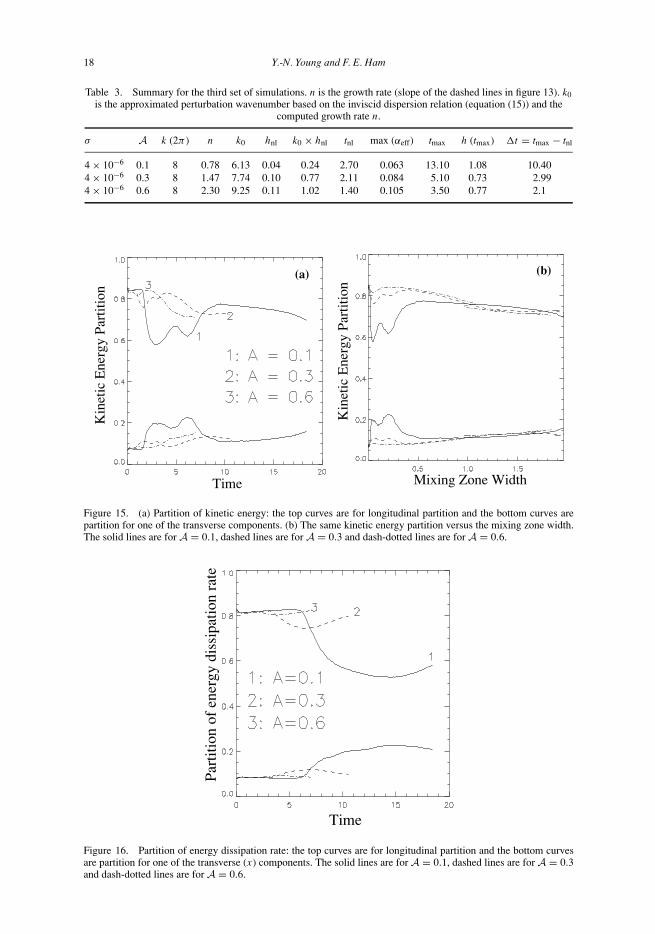
Figure 15. (a) Partition of kinetic energy: the top curves are for longitudinal partition and the bottom curves arepartition for one of the transverse components. (b) The same kinetic energy partition versus the mixing zone width.The solid lines are for A = 0.1, dashed lines are for A = 0.3 and dash-dotted lines are for A = 0.6.

Part

ition

of

ener

gy d

issi

patio

n ra

te

Time

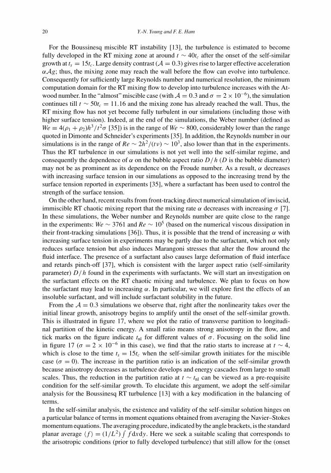
Figure 16. Partition of energy dissipation rate: the top curves are for longitudinal partition and the bottom curvesare partition for one of the transverse (x) components. The solid lines are for A = 0.1, dashed lines are for A = 0.3and dash-dotted lines are for A = 0.6.


altered by a smaller dominant perturbation wavelength λ, we repeat some of the simula-tions with the surface tension limited to a small value (σ = 4 × 10−6) due to the stabilizingeffects.

Figure 13 shows the bubble height and the effective mixing rate versus time, and table 3summarizes the basic characteristics of these simulations. The dominant wavelengths for allthese four simulations are around L/8. A transition to nonlinear evolution occurs at hnl ∼ 0.04for A = 0.1, while hnl ∼ 0.1 for both A = 0.3 and A = 0.6. Compared with the simulationsin section 4.2 with longer dominant perturbation wavelengths, we find the effective mixingrate αeff to be larger for smaller dominant wavelengths, and the mixing zone width at tmax

slightly depends on the Atwood number. The range of αeff in this set of simulations is similarto that in [7] with similar parameter values and range of perturbation wavelength. For example,the A = 0.3 run in table 3 has parameter values closest to those in [7] with a correspondingsurface tension σ ′ = 6 × 10−4. From the FronTier (front-tracking) simulations, the mixingrate αb ∼ 0.085 for σ ′ = 6 × 10−4 from figure 2 in [7], consistent with αeff = 0.073 fromour simulations. The fluid interface at tmax (when the maximum mixing rate is reached) isillustrated in figure 14 for all three cases.

Figure 15 shows the partition of kinetic energy, similar to the results for larger dominantperturbation wavelengths in section 4.2, the anisotropy in the RT turbulence is decreasing atthe end of the simulations. However, we observe stronger anisotropy for cases with smallerdominant perturbation wavelengths. Such stronger anisotropy is also reflected in the energydissipation rate in figure 16 (cf figure 12).

5. Conclusion

In this paper, we investigate the effect of surface tension on the RT instability and the ensuingmixing. For a single-mode RT instability, we modify the local potential flow analysis in [1]to consider the surface tension effect on the linear stability and the nonlinear terminal bubblevelocity. The stabilizing effect of surface tension on the linear growth rate is reproduced (thesame as in [21]). The terminal bubble velocity is reduced by surface tension, and these resultsare in good agreement with numerical simulations of a viscous, single-mode RT instabilitywith σ = 0.002.

We use the finite-volume, particle-level-set, two-phase flow solver to simulate RT mixingwith random perturbations at the interface. The homogeneous Cartesian grid refinement allowsus to accurately resolve the flow around the interface with a refined mesh. Such adaptivecapability also enables us to capture the interface dynamics efficiently without having to over-resolve the velocity away from the interface. We validate the usage of this code to simulate theimmiscible RT instability by comparing with results from the linear and nonlinear analyses.We also show numerical convergence in simulating the RT instability using the FV-PLS flowsolver.

We investigate the surface tension effect on the anisotropy in the RT mixing flow. Differentvalues of surface tension and density contrast are used in the simulations. In the RT mixingflow, the surface tension reduces the flow anisotropy, and redistributes some of the kineticenergy from the longitudinal component to the transverse components. For very small surfacetension (σ = 2 × 10−6), we simulate the “almost miscible” RT mixing with finite densitycontrast A = 0.3. Results from this simulation are consistent with those from Boussinesqmiscible RT simulations [13]; nonlinearity sets in at tnl before the initiation of self-similargrowth, which is around 15tc = 3.35. As the self-similar process begins, the effective mixingrate αeff first increases, reaches a maximum at tmax and then settles to an asymptotic constantif the conditions are sufficient for turbulence to develop.


For the Boussinesq miscible RT instability [13], the turbulence is estimated to becomefully developed in the RT mixing zone at around t ∼ 40tc after the onset of the self-similargrowth at ts = 15tc. Large density contrast (A = 0.3) gives rise to larger effective accelerationαAg; thus, the mixing zone may reach the wall before the flow can evolve into turbulence.Consequently for sufficiently large Reynolds number and numerical resolution, the minimumcomputation domain for the RT mixing flow to develop into turbulence increases with the At-wood number. In the “almost” miscible case (with A = 0.3 and σ = 2 × 10−6), the simulationcontinues till t ∼ 50tc = 11.16 and the mixing zone has already reached the wall. Thus, theRT mixing flow has not yet become fully turbulent in our simulations (including those withhigher surface tension). Indeed, at the end of the simulations, the Weber number (defined asWe ≡ 4(ρ1 + ρ2)h3/t2σ [35]) is in the range of We ∼ 800, considerably lower than the rangequoted in Dimonte and Schneider’s experiments [35]. In addition, the Reynolds number in oursimulations is in the range of Re ∼ 2h2/(tν) ∼ 103, also lower than that in the experiments.Thus the RT turbulence in our simulations is not yet well into the self-similar regime, andconsequently the dependence of α on the bubble aspect ratio D/h (D is the bubble diameter)may not be as prominent as its dependence on the Froude number. As a result, α decreaseswith increasing surface tension in our simulations as opposed to the increasing trend by thesurface tension reported in experiments [35], where a surfactant has been used to control thestrength of the surface tension.

On the other hand, recent results from front-tracking direct numerical simulation of inviscid,immiscible RT chaotic mixing report that the mixing rate α decreases with increasing σ [7].In these simulations, the Weber number and Reynolds number are quite close to the rangein the experiments: We ∼ 3761 and Re ∼ 105 (based on the numerical viscous dissipation intheir front-tracking simulations [36]). Thus, it is possible that the trend of increasing α withincreasing surface tension in experiments may be partly due to the surfactant, which not onlyreduces surface tension but also induces Marangoni stresses that alter the flow around thefluid interface. The presence of a surfactant also causes large deformation of fluid interfaceand retards pinch-off [37], which is consistent with the larger aspect ratio (self-similarityparameter) D/h found in the experiments with surfactants. We will start an investigation onthe surfactant effects on the RT chaotic mixing and turbulence. We plan to focus on howthe surfactant may lead to increasing α. In particular, we will explore first the effects of aninsoluble surfactant, and will include surfactant solubility in the future.

From the A = 0.3 simulations we observe that, right after the nonlinearity takes over theinitial linear growth, anisotropy begins to amplify until the onset of the self-similar growth.This is illustrated in figure 17, where we plot the ratio of transverse partition to longitudi-nal partition of the kinetic energy. A small ratio means strong anisotropy in the flow, andtick marks on the figure indicate tnl for different values of σ . Focusing on the solid linein figure 17 (σ = 2 × 10−6 in this case), we find that the ratio starts to increase at t ∼ 4,which is close to the time ts = 15tc when the self-similar growth initiates for the misciblecase (σ = 0). The increase in the partition ratio is an indication of the self-similar growthbecause anisotropy decreases as turbulence develops and energy cascades from large to smallscales. Thus, the reduction in the partition ratio at t ∼ tnl can be viewed as a pre-requisitecondition for the self-similar growth. To elucidate this argument, we adopt the self-similaranalysis for the Boussinesq RT turbulence [13] with a key modification in the balancing ofterms.

In the self-similar analysis, the existence and validity of the self-similar solution hinges ona particular balance of terms in moment equations obtained from averaging the Navier–Stokesmomentum equations. The averaging procedure, indicated by the angle brackets, is the standardplanar average 〈 f 〉 = (1/L2)

∫f dxdy. Here we seek a suitable scaling that corresponds to

the arisotropic conditions (prior to fully developed turbulence) that still allow for the (onset


Time

Rat

io o

f K

E p

artit

ion

Figure 17. Ratio of kinetic energy partition: x component to z component for A = 0.3 simulations. Solid line:σ = 2 × 10−6, dashed line: σ = 0.001, dash-dotted line: σ = 0.002 and dash-dot-dotted line: σ = 0.004. The tickmarks indicate the onset of nonlinearity tnl from table 1.

of the) self-similar solution. To this end, we find the following scaling:

∂t → ε∂t ′ , ∂x → εm∂x ′ , ∂y → εm∂y′ , ∂z → ε2∂z′ ,

p → p′

ε2, u → u′

εm−1, v → v′

εm−1, w → w′

ε, (33)

with ε � 1 and m > 1/2. Applying the above scaling with m = 1 to the first-order andsecond-order moment equations in [13], we obtain (dropping the primes)

〈w2〉z = −Pz − AgC, ∂t C + 〈wc〉z = 0, (34)

∂t 〈wc〉 + 〈w2c〉z = −〈w2〉Cz − Ag〈c2〉 − 〈cpz〉, (35)

∂t 〈c2〉 + 〈wc2〉z = −2〈wc〉Cz, (36)

∂t 〈w2〉 + 〈w3〉z = −2Ag〈wc〉 − 2〈wp〉z, (37)

−Ag〈wc〉 = 〈wp〉z, (38)

where P (mean pressure) and C (mean density) are the only non-zero first-order moments,and w and c are fluctuations in the longitudinal velocity and density, respectively. Due to thescaling (equation (33)) the molecular dissipative and diffusive terms in the original momentequations (equations (2.7)–(2.10) and (2.12) in [13]) drop out at leading order in ε. Applyingthe self-similar analysis in [13] to equations (34)–(38), we obtain the following self-similarsolution:

h(t ; C0, t0) = 1

4AgC0t2

0 (τ + 1)2, t0 =√

4h0

AgC0(39)

and other self-similar temporal behaviors that are found in [13]. Based on the above results,we conclude that the scaling in equation (33) implicates the strong anisotropy necessary for“cultivating” the onset of the self-similar turbulence. However, based on the turbulence theory,once the self-similar mixing starts the large-scale anisotropy will be reduced to small-scale


anisotropy or completely diminished for high enough Reynolds numbers. Thus, we can rea-sonably expect equation (33) to be a prelude to the self-similar growth in equation (39) andwe would not expect equation (33) to hold as turbulence develops. As a result, the scalingbehavior (such as w : u → 1 : ε) is an indicator for the onset of the self-similar RT turbulence.

We remark that the quadratic growth of the mixing zone h = αAgt2 may continue as longas there exists local velocity anisotropy (described by equation (33)) near the edge of themixing zone. In our future work, we will verify this and find a more rigorous condition for thedetection of the self-similar turbulence growth in the RT turbulence. Abarzhi et al. suggestedspecific scaling behavior for the self-similar turbulence; the vertical energy dissipation ratescales linearly with time, and the rate of momentum loss remains constant [33]. We willinvestigate these scaling behaviors in our numerical simulations of the RT turbulence, andinvestigate which one is the best indicator for the onset of the self-similar RT turbulence.

Acknowledgements

We acknowledge the support from the NSF/MRI funded computing cluster at NJIT/DMS. Wewish to thank J. Glimm, X. Li, Y. Zhang, P. Ramaprabhu and M. Siegel for helpful discussion.

References

[1] Goncharov, V.N., 2002, Physical Review Letters, 88, 134502.[2] Cook, A.W. and Dimotakis, P.E., 2001, Journal of Fluid Mechanics, 443, 69.[3] Ramaprabhu, P. and Andrews, M.J., 2004, Physics of Fluids, 16, L59.[4] Ramaprabhu, P., Dimonte, G. and Andrews, M.J., 2005, Journal of Fluid Mechanics, 536, 285.[5] Glimm, J., Grove, J.W., Li, X., Oh, W. and Sharp, D.H., 2001, Journal of Computational Physics, 169, 652.[6] Dimonte, G., Youngs, D.L., Dimits, A., Weber, S., Marinak, M., Wunsch, S., Garasi, C., Robinson, A., Andrews,

M.J., Ramaprabhu, P., et al., 2004, Physics of Fluids, 16, 1668.[7] George, E., Glimm, J., Li, X., Li, Y. and Liu, X., 2006, Physical Review E, 73, 016304.[8] Jin, H., Liu, X.F., Lu, T., Cheng, B., Glimm, J. and Sharp, D.H., 2005, Physics of Fluids, 17, 1.[9] Linden, P.F., Redondo, J.M. and Youngs, D.L., 1994, Journal of Fluid Mechanics, 265, 97.

[10] Dalziel, S.B., Linden, P.F. and Youngs, D.L., 1999, Journal of Fluid Mechanics, 399, 1.[11] Young, Y.-N., Tufo, H., Dubey, A. and Rosner, R., 2001, Journal of Fluid Mechanics, 447, 377.[12] Ramaprabhu, P. and Andrews, M.J., 2004, Journal of Fluid Mechanics, 502, 233.[13] Ristorcelli, J.R. and Clark, T.T., 2004, Journal of Fluid Mechanics, 507, 213.[14] Dimonte, G., 2004, Physical Review E, 69, 056305.[15] Chertkov, M., 2003, Physical Review Letters, 91, 115001.[16] Fermi, E., 1951, The Collected Papers of Enrico Fermi, In E. Segre (Ed.) vol. 2, pp. 816–821 (Chicago:

University of Chicago Press).[17] Layzer, D., 1955, Astrophysical Journal, 122, 1.[18] Hecht, J., Alon, U. and Shvarts, D., 1994, Physics of Fluids, 6, 4019.[19] Ramaprabhu, P. and Dimonte, G., 2005, Physical Review E, 71, 0363141.[20] Sohn, S.-I., 2004, Physical Review E, 69, 036703.[21] Chandrasekhar, S., 1961, Hydrodynamic and Hydromagnetic Instability (New York: Dover).[22] Ham, F.E., Lien, F.S. and Strong, A.B., 2002, Journal of Computational Physics, 179, 469.[23] Jiang, G.-S. and Peng, D., 2000, SIAM Journal of Scientific Computing, 21, 2126.[24] Enright, D., Fedkiw, R., Ferziger, J. and Mitchell, I., 2002, Journal of Computational Physics, 183, 83.[25] Young, Y.-N., Ferziger, J., Ham, F. and Herrmann, M., 2003, Center for Turbulence Research Annual Research

Briefs, http://ctr.stanford.edu/ResBriefs03/yyoung1.pdf[26] Sussman, M., Smereka, P. and Osher, S., 1994, Journal of Computational Physics, 114, 146.[27] Tornberg, A.-K., 2005, in Laptev, A. (ed.), European Congress of Mathematics (ECM), Stockholm, Sweden,

June 27–July 2, 2004. (Zurich: European Mathematical Society), pp. 477–429.[28] Kim, D. and Choi, H., 2000. Journal of Computational Physics, 162, 411.[29] Tryggvason, G., Bunner, B., Esmaeeli, A., Juric, D., Al-Rawahi, N., Tauber, W., Han, J., Nas, S. and Jan, Y.-J.,

2001, Journal of Computational Physics, 169, 708.[30] Clavin, P. and Williams, F., 2005, Journal of Fluid Mechanics, 525, 105.[31] Glimm, J., Li, X.-L. and Lin, A.-D., 2002, Acta Mathematicae Applicatea Sinica, 18, 1.[32] Ramaprabhu, P., Dimonte, G., Young, Y.-N., Fryxell, B. and Calder, A.C., 2005, in preparation.[33] Abarzhi, S.I., Gorobets, A. and Sreenivasan, K.R., 2005, Physics of Fluids, 17, 081705.


[34] Glimm, J., Grove, J.W., Li, X.L., Oh, W. and Sharp, D.H., 2001, Journal of Computational Physics, 169, 652.[35] Dimonte, G. and Schneider, M., 2000, Physics of Fluids, 12, 304.[36] Liu, X., 2006, private communication.[37] Stone, H.A., 1994, Annual Review of Fluid Mechanics, 26, 65.[38] Chertkov, M., Kolokolov, I. and Lebedev, V., 2005, Physical Review E, 71, 055301.[39] Cook, A.W. and Zhou, Y., 2002, Physical Review E, 66, 026312.

Documents

Surface tension in incompressible Rayleigh–Taylor mixing flowyyoung/young_papers/Young2006.pdf · The Rayleigh–Taylor (RT) instability is a fingering instability of fluid interface