Embed Size (px)
Citation preview
Survival Models
Lecture: Weeks 2-3
Lecture: Weeks 2-3 (STT 455) Survival Models Fall 2014 - Valdez 1 / 28
Chapter summary
Chapter summary
Survival models
Age-at-death random variable
Time-until-death random variables
Force of mortality (or hazard rate function)
Some parametric models
De Moivre’s (Uniform), Exponential, Weibull, Makeham, Gompertz
Generalization of De Moivre’s
Curtate future lifetime
Chapter 2 (Dickson, Hardy and Waters = DHW)
Lecture: Weeks 2-3 (STT 455) Survival Models Fall 2014 - Valdez 2 / 28
Age-at-death survival function
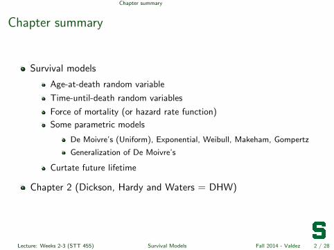
Age-at-death random variable
X is the age-at-death random variable; continuous, non-negative
X is interpreted as the lifetime of a newborn (individual from birth)
Distribution of X is often described by its survival distributionfunction (SDF):
S0(x) = Pr[X > x]
other term used: survival function
Properties of the survival function:
S0(0) = 1: probability a newborn survives 0 years is 1.
S0(∞) = limx→∞ S0(x) = 0: all lives eventually die.
non-increasing function of x: not possible to have a higher probabilityof surviving for a longer period.
Lecture: Weeks 2-3 (STT 455) Survival Models Fall 2014 - Valdez 3 / 28
Produced with a Trial Version of PDF Annotator - www.PDFAnnotator.com

Age-at-death CDF and density
Cumulative distribution and density functions
Cumulative distribution function (CDF): F0(x) = Pr[X ≤ x]
nondecreasing; F0(0) = 0; and F0(∞) = 1.
Clearly we have: F0(x) = 1− S0(x)
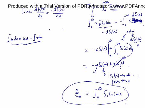
Density function: f0 (x) =dF0(x)dx
= −dS0(x)dx
non-negative: f0(x) ≥ 0 for any x ≥ 0
in terms of CDF: F0(x) =∫ x
0
f0(z)dz
in terms of SDF: S0(x) =∫ ∞
x
f0(z)dz
Lecture: Weeks 2-3 (STT 455) Survival Models Fall 2014 - Valdez 4 / 28
Produced with a Trial Version of PDF Annotator - www.PDFAnnotator.com
Age-at-death force of mortality
Force of mortality
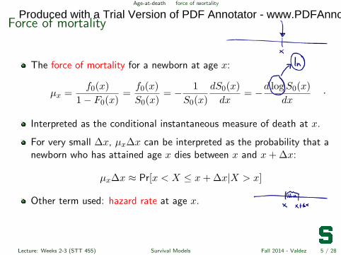
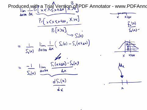
The force of mortality for a newborn at age x:
µx =f0(x)
1− F0(x)=f0(x)S0(x)
= − 1S0(x)
dS0(x)dx
= −d logS0(x)dx
Interpreted as the conditional instantaneous measure of death at x.
For very small ∆x, µx∆x can be interpreted as the probability that anewborn who has attained age x dies between x and x+ ∆x:
µx∆x ≈ Pr[x < X ≤ x+ ∆x|X > x]
Other term used: hazard rate at age x.
Lecture: Weeks 2-3 (STT 455) Survival Models Fall 2014 - Valdez 5 / 28
Produced with a Trial Version of PDF Annotator - www.PDFAnnotator.com
Produced with a Trial Version of PDF Annotator - www.PDFAnnotator.com
Age-at-death force of mortality
Some properties of µx
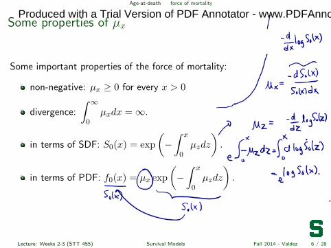
Some important properties of the force of mortality:
non-negative: µx ≥ 0 for every x > 0
divergence:
∫ ∞
0µxdx =∞.
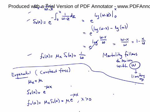
in terms of SDF: S0(x) = exp(−∫ x
0µzdz
).
in terms of PDF: f0(x) = µx exp(−∫ x
0µzdz
).
Lecture: Weeks 2-3 (STT 455) Survival Models Fall 2014 - Valdez 6 / 28
Produced with a Trial Version of PDF Annotator - www.PDFAnnotator.com
Produced with a Trial Version of PDF Annotator - www.PDFAnnotator.com
Age-at-death moments
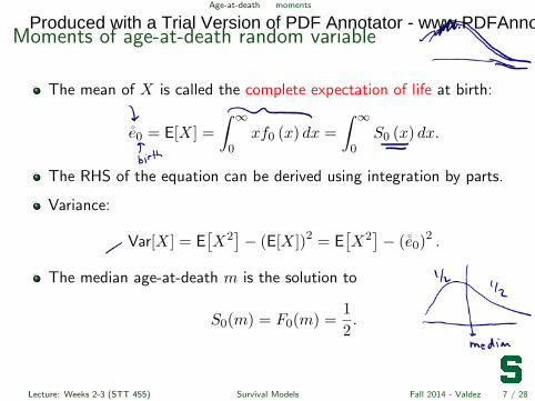
Moments of age-at-death random variable
The mean of X is called the complete expectation of life at birth:
e̊0 = E[X] =∫ ∞
0xf0 (x) dx =
∫ ∞
0S0 (x) dx.
The RHS of the equation can be derived using integration by parts.
Variance:
Var[X] = E[X2]− (E[X])2 = E
[X2]− (̊e0)2 .
The median age-at-death m is the solution to
S0(m) = F0(m) =12.
Lecture: Weeks 2-3 (STT 455) Survival Models Fall 2014 - Valdez 7 / 28
Produced with a Trial Version of PDF Annotator - www.PDFAnnotator.com
Produced with a Trial Version of PDF Annotator - www.PDFAnnotator.com
Special laws of mortality
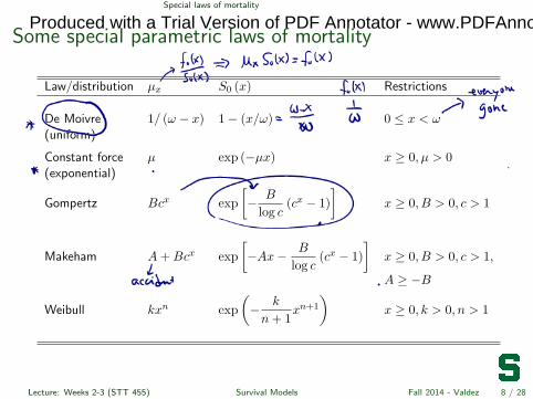
Some special parametric laws of mortality
Law/distribution µx S0 (x) Restrictions
De Moivre 1/ (ω − x) 1− (x/ω) 0 ≤ x < ω(uniform)
Constant force µ exp (−µx) x ≥ 0, µ > 0(exponential)
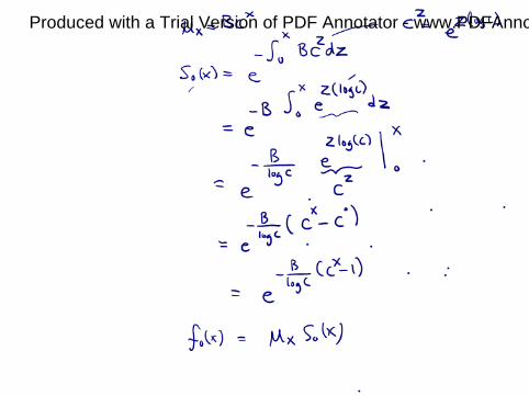
Gompertz Bcx exp[− B
log c(cx − 1)
]x ≥ 0, B > 0, c > 1
Makeham A+Bcx exp[−Ax− B
log c(cx − 1)
]x ≥ 0, B > 0, c > 1,
A ≥ −B
Weibull kxn exp(− k
n+ 1xn+1
)x ≥ 0, k > 0, n > 1
Lecture: Weeks 2-3 (STT 455) Survival Models Fall 2014 - Valdez 8 / 28
Produced with a Trial Version of PDF Annotator - www.PDFAnnotator.com
Produced with a Trial Version of PDF Annotator - www.PDFAnnotator.com
Produced with a Trial Version of PDF Annotator - www.PDFAnnotator.com
Special laws of mortality
0 20 40 60 80 100 120
0.0
0.5
1.0
1.5
2.0
2.5
3.0
force of mortality
x
mu(
x)
0 20 40 60 80 100 120
0.0
0.2
0.4
0.6
0.8
1.0
survival function
x
surv
(x)
0 20 40 60 80 100 120
0.0
0.2
0.4
0.6
0.8
1.0
distribution function
x
dist(x
)
0 20 40 60 80 100 120
0.00
00.
010
0.02
00.
030
density function
x
dens
(x)
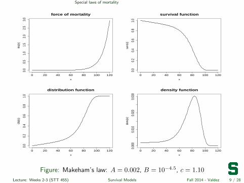
Figure: Makeham’s law: A = 0.002, B = 10−4.5, c = 1.10Lecture: Weeks 2-3 (STT 455) Survival Models Fall 2014 - Valdez 9 / 28
Special laws of mortality illustrative example 1
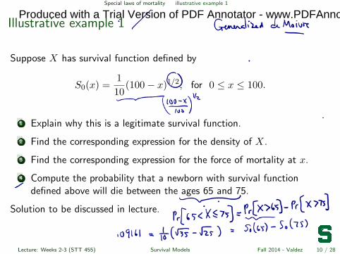
Illustrative example 1
Suppose X has survival function defined by
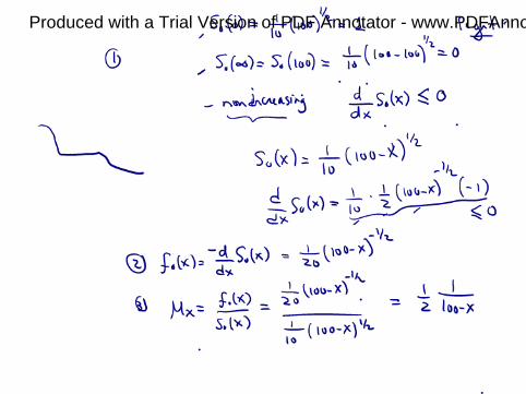
S0(x) =110
(100− x)1/2, for 0 ≤ x ≤ 100.
1 Explain why this is a legitimate survival function.
2 Find the corresponding expression for the density of X.
3 Find the corresponding expression for the force of mortality at x.
4 Compute the probability that a newborn with survival functiondefined above will die between the ages 65 and 75.
Solution to be discussed in lecture.
Lecture: Weeks 2-3 (STT 455) Survival Models Fall 2014 - Valdez 10 / 28
Produced with a Trial Version of PDF Annotator - www.PDFAnnotator.com
Produced with a Trial Version of PDF Annotator - www.PDFAnnotator.com
Time-until-death
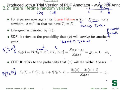
2.2 Future lifetime random variable
For a person now age x, its future lifetime is Tx = X − x. For anewborn, x = 0, so that we have T0 = X.
Life-age-x is denoted by (x).
SDF: It refers to the probability that (x) will survive for another tyears.
Sx(t) = Pr[T0 > x+ t|T0 > x] =S0(x+ t)S0(x)
= pt x = 1− qt x
CDF: It refers to the probability that (x) will die within t years.
Fx(t) = Pr[T0 ≤ x+ t|T0 > x] =S0(x)− S0(x+ t)
S0(x)= qt x
Lecture: Weeks 2-3 (STT 455) Survival Models Fall 2014 - Valdez 11 / 28
Produced with a Trial Version of PDF Annotator - www.PDFAnnotator.com


Time-until-death
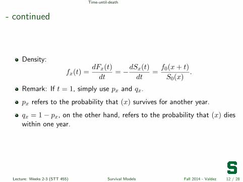
- continued
Density:
fx(t) =dFx(t)dt
= −dSx(t)dt
=f0(x+ t)S0(x)
.
Remark: If t = 1, simply use px and qx.
px refers to the probability that (x) survives for another year.
qx = 1− px, on the other hand, refers to the probability that (x) dieswithin one year.
Lecture: Weeks 2-3 (STT 455) Survival Models Fall 2014 - Valdez 12 / 28
Time-until-death force of mortality
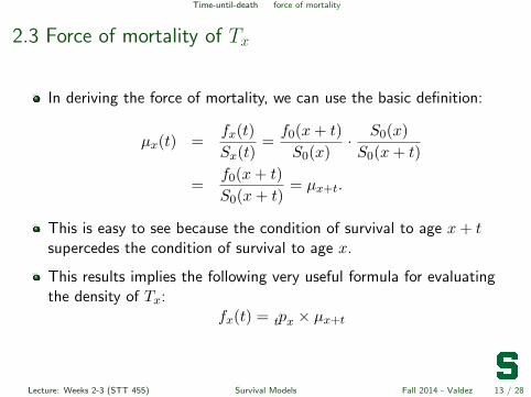
2.3 Force of mortality of Tx
In deriving the force of mortality, we can use the basic definition:
µx(t) =fx(t)Sx(t)
=f0(x+ t)S0(x)
· S0(x)S0(x+ t)
=f0(x+ t)S0(x+ t)
= µx+t.
This is easy to see because the condition of survival to age x+ tsupercedes the condition of survival to age x.
This results implies the following very useful formula for evaluatingthe density of Tx:
fx(t) = pt x × µx+t
Lecture: Weeks 2-3 (STT 455) Survival Models Fall 2014 - Valdez 13 / 28
Time-until-death 2.4 special probability symbol
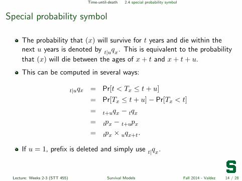
Special probability symbol
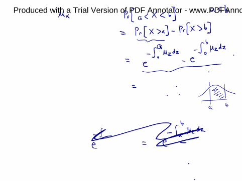
The probability that (x) will survive for t years and die within thenext u years is denoted by qt|u x. This is equivalent to the probability
that (x) will die between the ages of x+ t and x+ t+ u.
This can be computed in several ways:
t|uqx = Pr[t < Tx ≤ t+ u]= Pr[Tx ≤ t+ u]− Pr[Tx < t]= qt+u x − qt x
= pt x − pt+u x
= pt x × qu x+t.
If u = 1, prefix is deleted and simply use qt| x.
Lecture: Weeks 2-3 (STT 455) Survival Models Fall 2014 - Valdez 14 / 28
Time-until-death
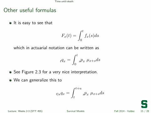
Other useful formulas
It is easy to see that
Fx(t) =∫ t
0fx(s)ds
which in actuarial notation can be written as
qt x =∫ t
0ps x µx+sds
See Figure 2.3 for a very nice interpretation.
We can generalize this to
t|uqx =∫ t+u
tps x µx+sds
Lecture: Weeks 2-3 (STT 455) Survival Models Fall 2014 - Valdez 15 / 28


Lecture: Weeks 2-3 (STT 455) Survival Models Fall 2014 - Valdez
Time-until-death curtate future lifetime
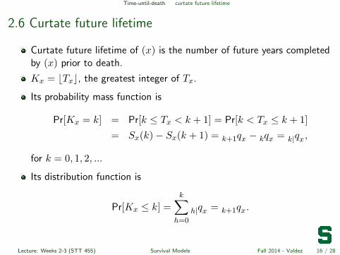
2.6 Curtate future lifetime
Curtate future lifetime of (x) is the number of future years completedby (x) prior to death.
Kx = bTxc, the greatest integer of Tx.
Its probability mass function is
Pr[Kx = k] = Pr[k ≤ Tx < k + 1] = Pr[k < Tx ≤ k + 1]= Sx(k)− Sx(k + 1) = qk+1 x − qk x = qk| x,
for k = 0, 1, 2, ...
Its distribution function is
Pr[Kx ≤ k] =k∑
h=0
qh| x = qk+1 x.
Lecture: Weeks 2-3 (STT 455) Survival Models Fall 2014 - Valdez 16 / 28


Expectation of life
2.5/2.6 Expectation of life
The expected value of Tx is called the complete expectation of life:
e̊x = E[Tx] =∫ ∞
0tfx(t)dt =
∫ ∞
0t pt xµx+tdt =
∫ ∞
0pt xdt.
The expected value of Kx is called the curtate expectation of life:
ex = E[Kx] =∞∑k=0
k · Pr[Kx = k] =∞∑k=0
k · qk| x =∞∑k=1
pk x.
Proof can be derived using discrete counterpart of integration by parts(summation by parts). Alternative proof will be provided in class.
Variances of future lifetime can be similarly defined.
Lecture: Weeks 2-3 (STT 455) Survival Models Fall 2014 - Valdez 17 / 28


Expectation of life Examples
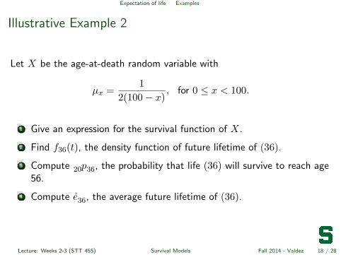
Illustrative Example 2
Let X be the age-at-death random variable with
µx =1
2(100− x), for 0 ≤ x < 100.
1 Give an expression for the survival function of X.
2 Find f36(t), the density function of future lifetime of (36).
3 Compute p20 36, the probability that life (36) will survive to reach age56.
4 Compute e̊36, the average future lifetime of (36).
Lecture: Weeks 2-3 (STT 455) Survival Models Fall 2014 - Valdez 18 / 28


Expectation of life Examples
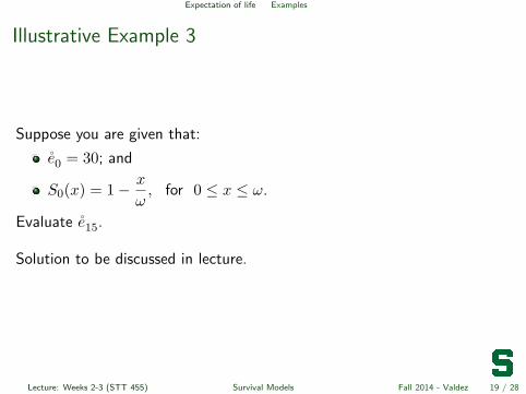
Illustrative Example 3
Suppose you are given that:
e̊0 = 30; and
S0(x) = 1− x
ω, for 0 ≤ x ≤ ω.
Evaluate e̊15.
Solution to be discussed in lecture.
Lecture: Weeks 2-3 (STT 455) Survival Models Fall 2014 - Valdez 19 / 28
Lecture: Weeks 2-3 (STT 455) Survival Models Fall 2014 - Valdez

Lecture: Weeks 2-3 (STT 455) Survival Models Fall 2014 - Valdez
Expectation of life Examples
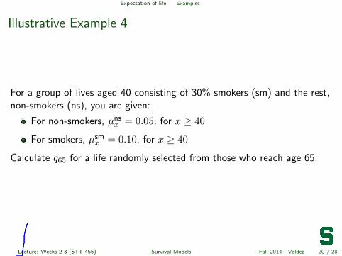
Illustrative Example 4
For a group of lives aged 40 consisting of 30% smokers (sm) and the rest,non-smokers (ns), you are given:
For non-smokers, µnsx = 0.05, for x ≥ 40
For smokers, µsmx = 0.10, for x ≥ 40
Calculate q65 for a life randomly selected from those who reach age 65.
Lecture: Weeks 2-3 (STT 455) Survival Models Fall 2014 - Valdez 20 / 28

Lecture: Weeks 2-3 (STT 455) Survival Models Fall 2014 - Valdez

Lecture: Weeks 2-3 (STT 455) Survival Models Fall 2014 - Valdez
Expectation of life
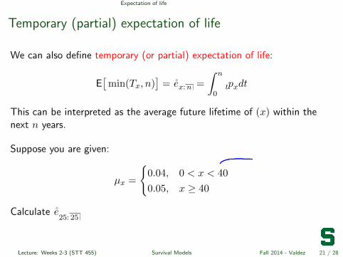
Temporary (partial) expectation of life
We can also define temporary (or partial) expectation of life:
E[
min(Tx, n)]
= e̊x:n =∫ n
0pt xdt
This can be interpreted as the average future lifetime of (x) within thenext n years.
Suppose you are given:
µx =
{0.04, 0 < x < 400.05, x ≥ 40
Calculate e̊25: 25
Lecture: Weeks 2-3 (STT 455) Survival Models Fall 2014 - Valdez 21 / 28

Lecture: Weeks 2-3 (STT 455) Survival Models Fall 2014 - Valdez
Lecture: Weeks 2-3 (STT 455) Survival Models Fall 2014 - Valdez
Expectation of life generalized De Moivre’s
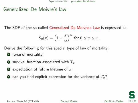
Generalized De Moivre’s law
The SDF of the so-called Generalized De Moivre’s Law is expressed as
S0(x) =(
1− x
ω
)αfor 0 ≤ x ≤ ω.
Derive the following for this special type of law of mortality:
1 force of mortality
2 survival function associated with Tx
3 expectation of future lifetime of x
4 can you find explicit expression for the variance of Tx?
Lecture: Weeks 2-3 (STT 455) Survival Models Fall 2014 - Valdez 22 / 28

Lecture: Weeks 2-3 (STT 455) Survival Models Fall 2014 - Valdez

Lecture: Weeks 2-3 (STT 455) Survival Models Fall 2014 - Valdez

Lecture: Weeks 2-3 (STT 455) Survival Models Fall 2014 - Valdez

Lecture: Weeks 2-3 (STT 455) Survival Models Fall 2014 - Valdez
generalized De Moivre’s illustrative example
Illustrative example
We will do Example 2.6 in class.
Lecture: Weeks 2-3 (STT 455) Survival Models Fall 2014 - Valdez 23 / 28
Gompertz law example 2.3
Example 2.3
Let µx = Bcx, for x > 0, where B and c are constants such that0 < B < 1 and c > 1.
Derive an expression for Sx(t).
Lecture: Weeks 2-3 (STT 455) Survival Models Fall 2014 - Valdez 24 / 28

Lecture: Weeks 2-3 (STT 455) Survival Models Fall 2014 - Valdez

Lecture: Weeks 2-3 (STT 455) Survival Models Fall 2014 - Valdez

Lecture: Weeks 2-3 (STT 455) Survival Models Fall 2014 - Valdez

Lecture: Weeks 2-3 (STT 455) Survival Models Fall 2014 - Valdez
Others typical mortality
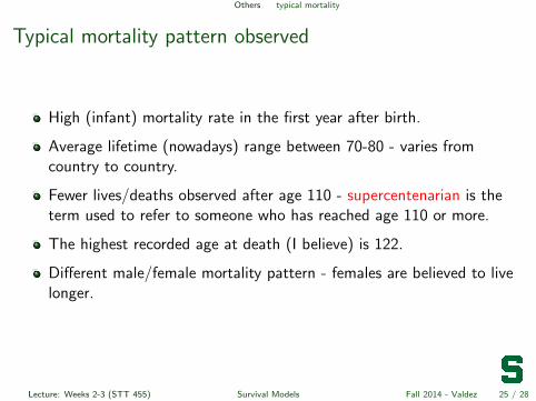
Typical mortality pattern observed
High (infant) mortality rate in the first year after birth.
Average lifetime (nowadays) range between 70-80 - varies fromcountry to country.
Fewer lives/deaths observed after age 110 - supercentenarian is theterm used to refer to someone who has reached age 110 or more.
The highest recorded age at death (I believe) is 122.
Different male/female mortality pattern - females are believed to livelonger.
Lecture: Weeks 2-3 (STT 455) Survival Models Fall 2014 - Valdez 25 / 28
Others substandard mortality
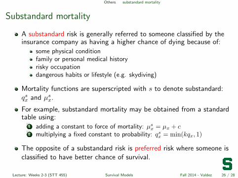
Substandard mortality
A substandard risk is generally referred to someone classified by theinsurance company as having a higher chance of dying because of:
some physical conditionfamily or personal medical historyrisky occupationdangerous habits or lifestyle (e.g. skydiving)
Mortality functions are superscripted with s to denote substandard:qsx and µsx.
For example, substandard mortality may be obtained from a standardtable using:
1 adding a constant to force of mortality: µsx = µx + c
2 multiplying a fixed constant to probability: qsx = min(kqx, 1)
The opposite of a substandard risk is preferred risk where someone isclassified to have better chance of survival.
Lecture: Weeks 2-3 (STT 455) Survival Models Fall 2014 - Valdez 26 / 28

Lecture: Weeks 2-3 (STT 455) Survival Models Fall 2014 - Valdez
Final remark
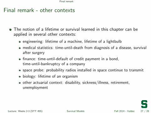
Final remark - other contexts
The notion of a lifetime or survival learned in this chapter can beapplied in several other contexts:
engineering: lifetime of a machine, lifetime of a lightbulb
medical statistics: time-until-death from diagnosis of a disease, survivalafter surgery
finance: time-until-default of credit payment in a bond,time-until-bankruptcy of a company
space probe: probability radios installed in space continue to transmit
biology: lifetime of an organism
other actuarial context: disability, sickness/illness, retirement,unemployment
Lecture: Weeks 2-3 (STT 455) Survival Models Fall 2014 - Valdez 27 / 28
Final remark other notations
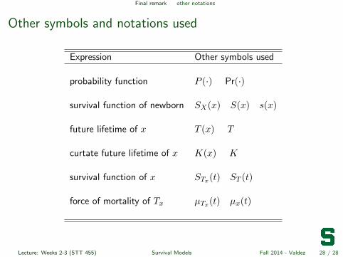
Other symbols and notations used
Expression Other symbols used
probability function P (·) Pr(·)
survival function of newborn SX(x) S(x) s(x)
future lifetime of x T (x) T
curtate future lifetime of x K(x) K
survival function of x STx(t) ST (t)
force of mortality of Tx µTx(t) µx(t)
Lecture: Weeks 2-3 (STT 455) Survival Models Fall 2014 - Valdez 28 / 28

![Survival Analysis - University of Washingtonfaculty.washington.edu/heagerty/Courses/VA-survival/...It’s life and death... Survival function: S(t) = P [T > t] The survival function](https://img.pdfslide.net/doc/110x75/611600f94ef3f41cc655565e/survival-analysis-university-of-itas-life-and-death-survival-function.jpg)