Embed Size (px)
Citation preview
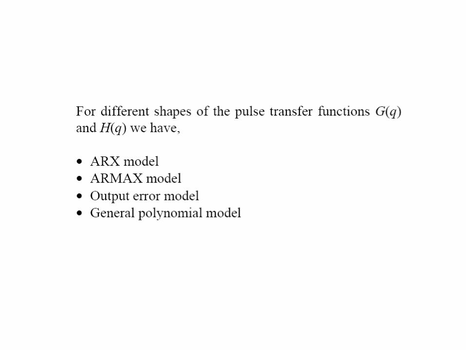
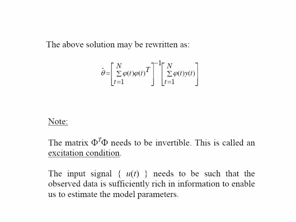
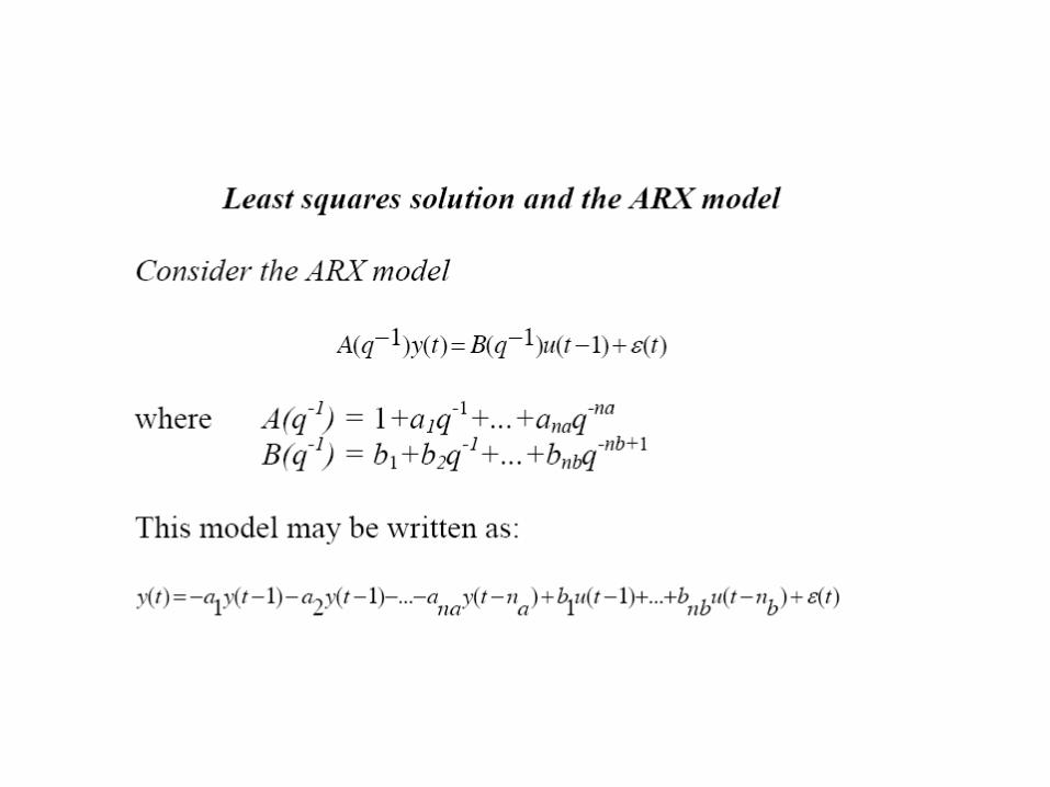
System identification and self regulating systems

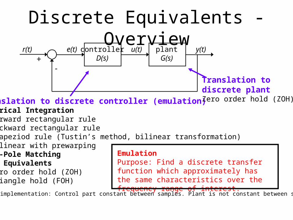
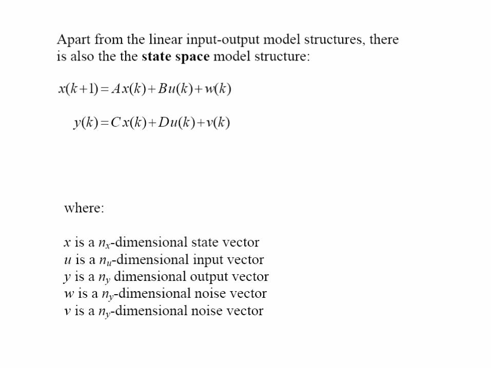
Discrete Equivalents - Overviewcontroller
D(s)plantG(s)
r(t) u(t) y(t)e(t)+
-
Translation to discrete controller (emulation)Numerical Integration• Forward rectangular rule• Backward rectangular rule• Trapeziod rule (Tustin’s method, bilinear transformation)• Bilinear with prewarpingZero-Pole MatchingHold Equivalents• Zero order hold (ZOH)• Triangle hold (FOH)
Translation todiscrete plantZero order hold (ZOH)
EmulationPurpose: Find a discrete transfer function which approximately has the same characteristics over the frequency range of interest.
Digital implementation: Control part constant between samples. Plant is not constant between samples.
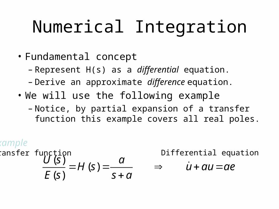
Numerical Integration
• Fundamental concept– Represent H(s) as a differential equation.– Derive an approximate difference equation.
• We will use the following example– Notice, by partial expansion of a transfer function this
example covers all real poles.
aeauuas
asH
sE
sU
)(
)(
)(
ExampleTransfer function Differential equation
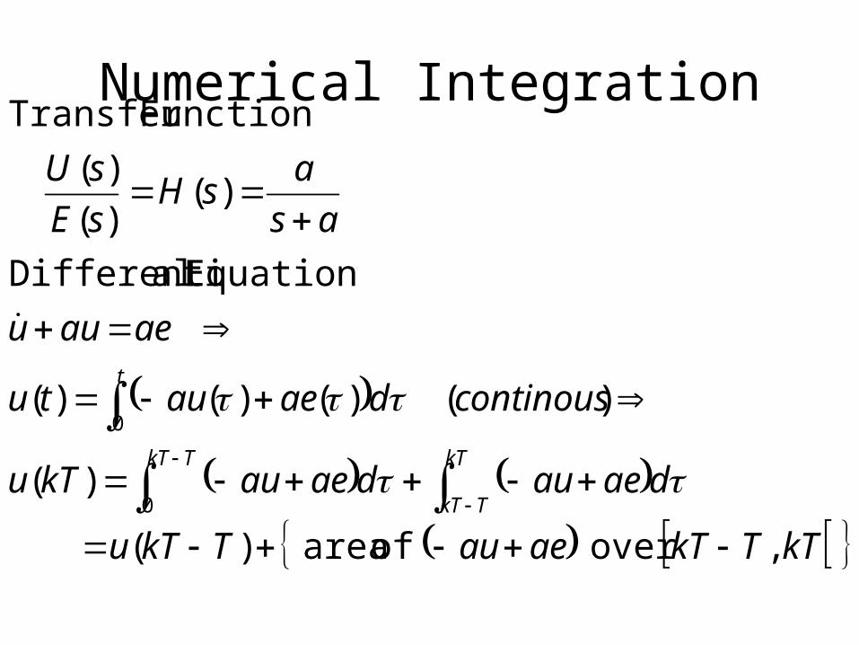
Numerical Integration
kTTkTaeauTkTu
daeaudaeaukTu
continousdaeautu
aeauu
as
asH
sE
sU
TkT kT
TkT
t
,over of area)(
)(
)()()()(
Equation alDifferenti
)()(
)(
FunctionTransfer
0
0
Numerical Integration
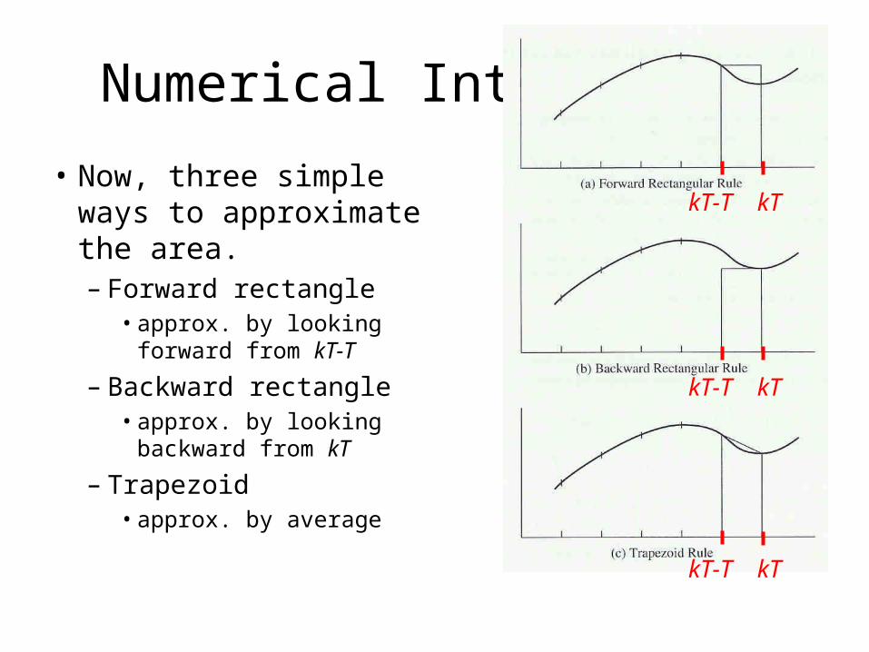
• Now, three simple ways to approximate the area.– Forward rectangle
• approx. by looking forward from kT-T
– Backward rectangle• approx. by looking
backward from kT
– Trapezoid• approx. by average
kT-T kT
kT-T kT
kT-T kT
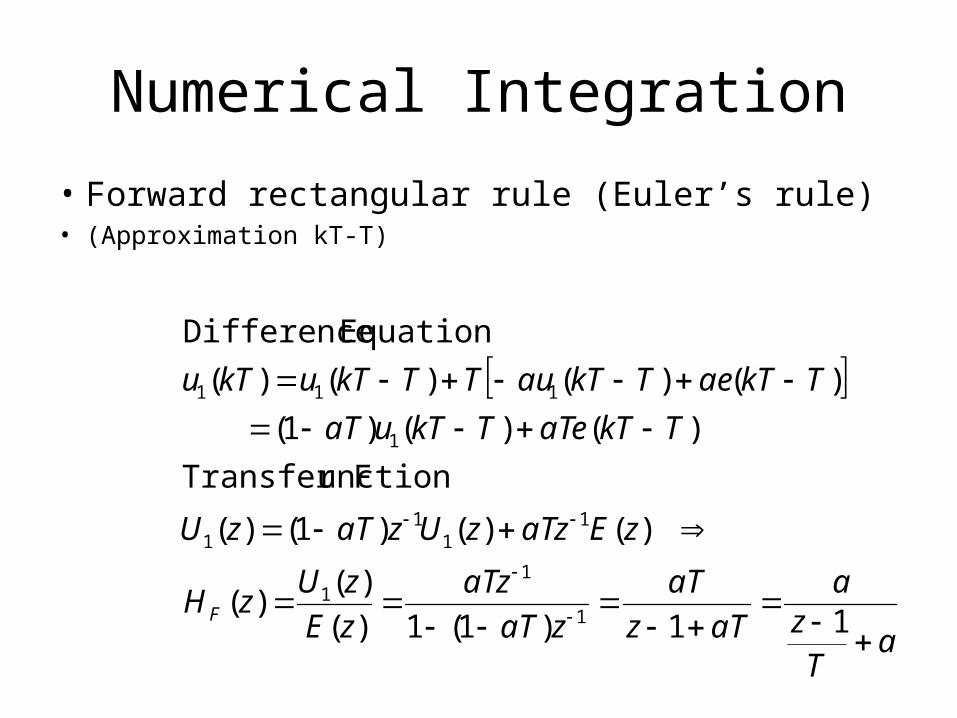
Numerical Integration
• Forward rectangular rule (Euler’s rule)• (Approximation kT-T)
aTza
aTz
aT
zaT
aTz
zE
zUzH
zEaTzzUzaTzU
TkTaTeTkTuaT
TkTaeTkTauTTkTukTu
F
11)1(1)(
)()(
)()()1()(
unctionTransfer F
)()()1(
)()()()(
EquationDifference
1
11
11
11
1
111
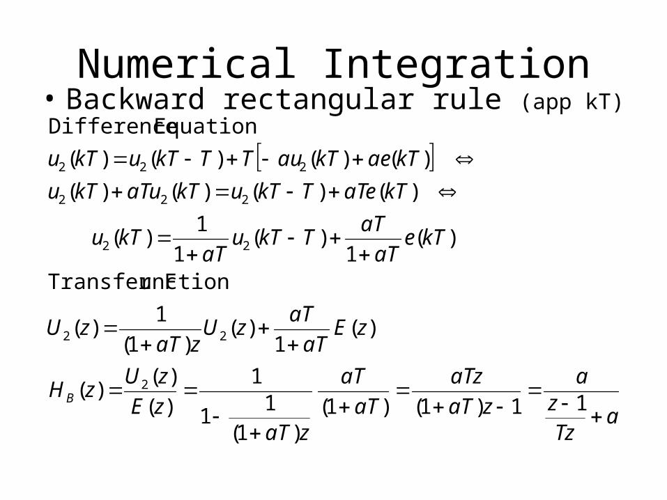
Numerical Integration• Backward rectangular rule (app kT)
aTzza
zaT
aTz
aT
aT
zaTzE
zUzH
zEaT
aTzU
zaTzU
kTeaT
aTTkTu
aTkTu
kTaTeTkTukTaTukTu
kTaekTauTTkTukTu
B
11)1()1()1(
11
1
)(
)()(
)(1
)()1(
1)(
unctionTransfer F
)(1
)(1
1)(
)()()()(
)()()()(
EquationDifference
2
22
22
222
222
Numerical Integration
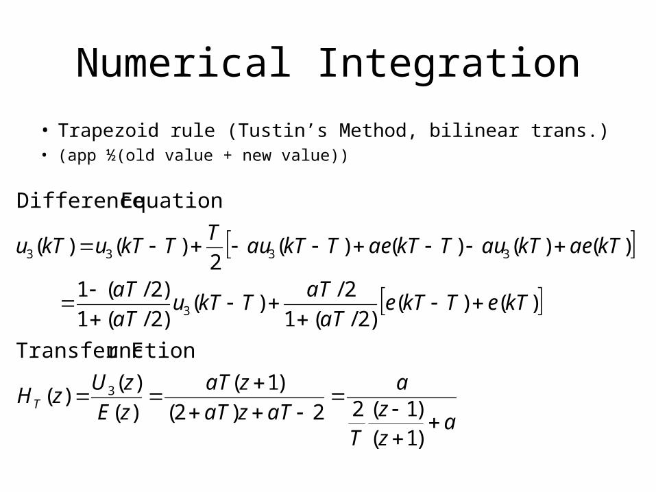
• Trapezoid rule (Tustin’s Method, bilinear trans.)• (app ½(old value + new value))
azz
T
a
aTzaT
zaT
zE
zUzH
kTeTkTeaT
aTTkTu
aT
aT
kTaekTauTkTaeTkTauT
TkTukTu
T
)1()1(22)2(
)1(
)(
)()(
unctionTransfer F
)()()2/(1
2/)(
)2/(1
)2/(1
)()()()(2
)()(
EquationDifference
3
3
3333
Numerical Integration
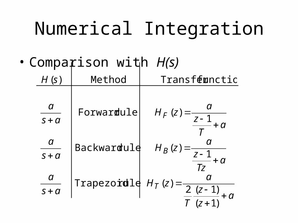
• Comparison with H(s)
azz
T
azH
as
a
aTzza
zHas
a
aTza
zHas
a
sH
T
B
F
)1()1(2
)(rule Trapezoid
1)(rule Backward
1)(rule Forward
functionTransfer Method)(
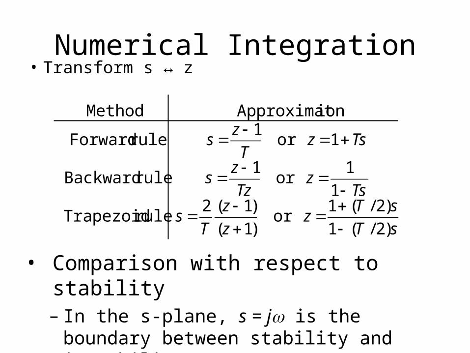
Numerical Integration• Transform s ↔ z
sT
sTz
z
z
Ts
Tsz
Tz
zs
TszT
zs
)2/(1
)2/(1or
)1(
)1(2rule Trapezoid
1
1or
1rule Backward
1or1
rule Forward
ionApproximatMethod
• Comparison with respect to stability– In the s-plane, s = j is the boundary between
stability and instability.

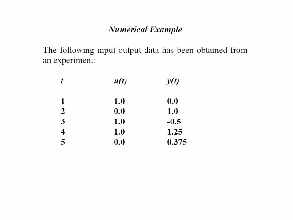
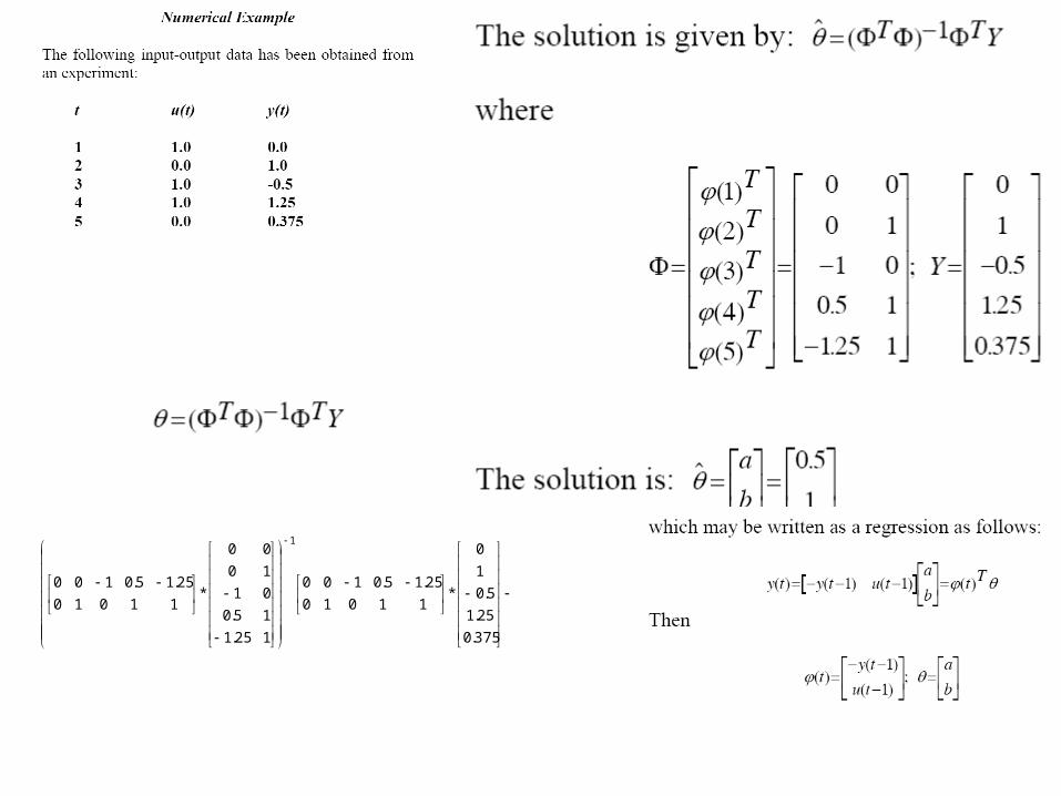
375.0
25.1
5.0
1
0
*11010
25.15.0100
125.1
15.0
01
10
00
*11010
25.15.0100
1
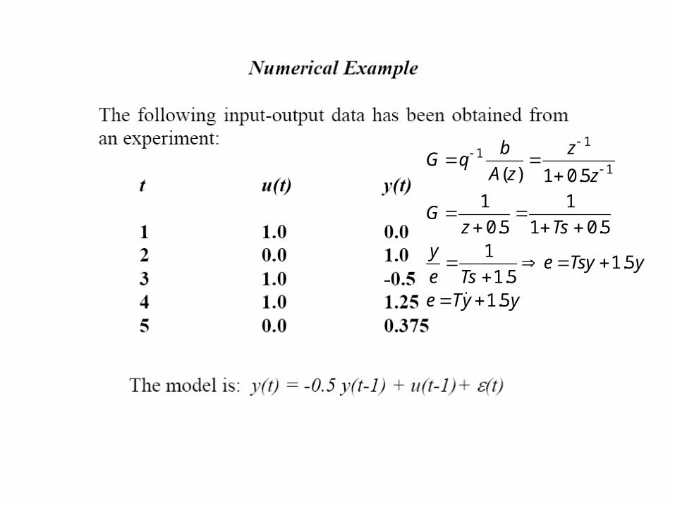
yyTe
yTsyeTse
yTsz
G
z
z
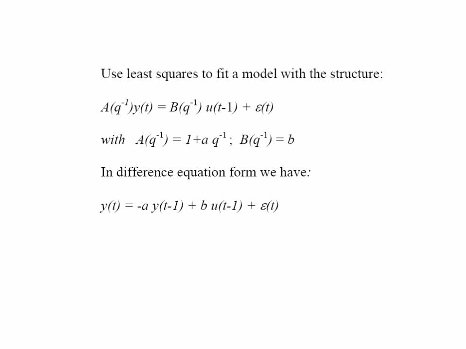
zA
bqG
5.1
5.15.1
15.01
1
5.0
1
5.01)( 1
11
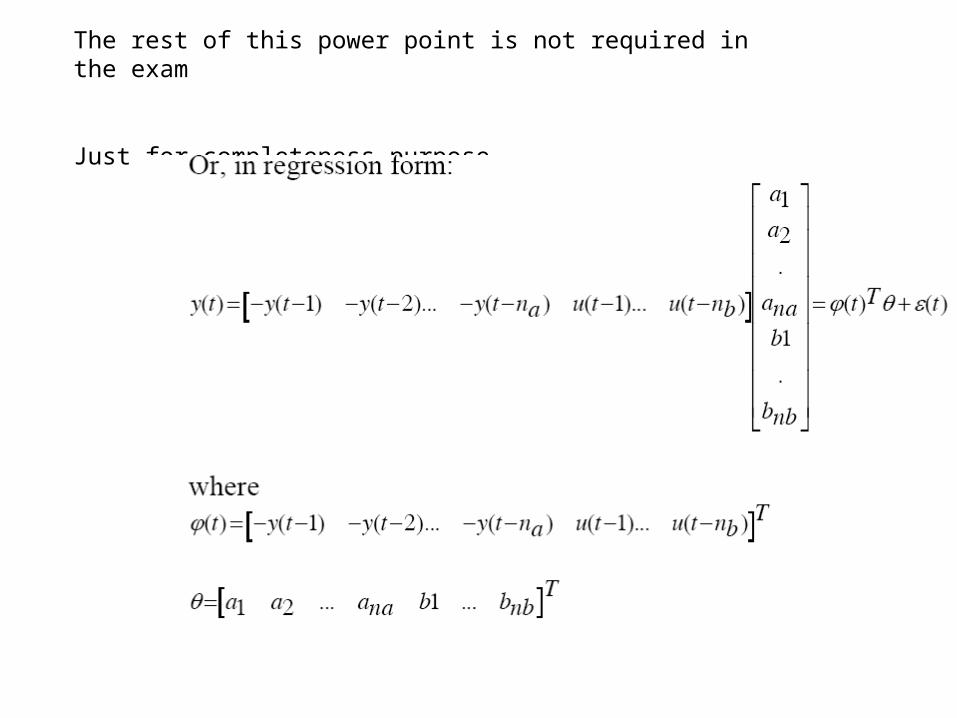
The rest of this power point is not required in the exam
Just for completeness purpose