Embed Size (px)
Citation preview
HAL Id: hal-01181163https://hal.archives-ouvertes.fr/hal-01181163
Submitted on 29 Jul 2015
HAL is a multi-disciplinary open accessarchive for the deposit and dissemination of sci-entific research documents, whether they are pub-lished or not. The documents may come fromteaching and research institutions in France orabroad, or from public or private research centers.
L’archive ouverte pluridisciplinaire HAL, estdestinée au dépôt et à la diffusion de documentsscientifiques de niveau recherche, publiés ou non,émanant des établissements d’enseignement et derecherche français ou étrangers, des laboratoirespublics ou privés.
Systematic LFT Derivation of Uncertain ElectricalCircuits for the Worst-Case Tolerance Analysis
Moises Ferber de Vieira Lessa, Anton Korniienko, Gérard Scorletti, ChristianVollaire, Florent Morel, Laurent Krähenbühl
To cite this version:Moises Ferber de Vieira Lessa, Anton Korniienko, Gérard Scorletti, Christian Vollaire, Florent Morel,et al.. Systematic LFT Derivation of Uncertain Electrical Circuits for the Worst-Case ToleranceAnalysis. IEEE Transactions on Electromagnetic Compatibility, Institute of Electrical and ElectronicsEngineers, 2015, 57 (5), pp.937 - 946. 10.1109/TEMC.2015.2419455. hal-01181163
Systematic LFT Derivation of Uncertain
Electrical Circuits for Worst-Case Tolerance
AnalysisMoises Ferber∗†, Anton Korniienko∗, Gerard Scorletti∗, Christian Vollaire∗, Florent Morel∗, Laurent
Krahenbuhl∗,∗University of Lyon, ECL
Ampere, CNRS UMR5005, 36 avenue Guy de Collongue, 69134 Ecully, France
Email: [email protected]†Laboratorio de Computacao Evolucionaria
Universidade Federal de Minas Gerais, Belo Horizonte, Brazil
Abstract
In line with the trend towards continuous miniaturization and price reduction, it is crucial to analyze the impact
of uncertainties on the performance of electrical circuits. Performance is evaluated for the worst-case scenario and
in the frequency domain, by computing upper and lower bounds. The purpose is not only to propose a method for
the worst-case tolerance analysis but also to provide an efficient and a suitable tool for electrical engineers that can
be easily applied to realistic electrical engineering problems. The proposed method is based on the robust analysis
method (so called µ-analysis) for which well-known and efficient algorithms exist. However in order to apply it, the
problem under consideration has to be transformed in a standard minimal so called LFT representation. Its derivation
is a difficult task even for control systems engineers. Our paper proposes a transparent and systematic LFT derivation
procedure for users based only on their knowledge of electrical engineering. At the end of the paper, an industrial
example is provided which reveals the benefits and the efficiency of the proposed approach and how it can be applied
to any linear electrical circuit.
Index Terms
Linear Fractional Transformation, Robustness analysis of circuits, uncertainty, worst-case analysis, µ-analysis,
ν-analysis.
I. INTRODUCTION
Nowadays, the semiconductor industry continuously scales toward nanometer technologies while constantly
increasing complexity and deep silicon integration of electrical circuits. Both important technological dispersions and
increase of interconnection parameter variations can bring a significant degradation of electrical circuit performance.
In order to design a reliable system, it is thus required to take these parameter variations into account and to ensure
the robust performance of the circuit besides the nominal one. The robust performance analysis is the procedure
allowing to test whether the system performance remains to be acceptable in front of possible parameter variations
or model uncertainties.
There can be underlined two existing approaches to achieve the mentioned goal: (i) probabilistic and (ii) worst-
case analysis methodologies. The first approach allows to determine the probability of robust performance based
on the given probability density functions (PDF) over parameters [1]–[5]. The worst-case approach in its turn does
not consider any probabilistic aspects and the performance criteria is analyzed for the worst combination of the
uncertain parameters [3], [6]–[10]. It ensures the robust performance for all possible combination of the uncertain
parameters.
In some critical applications such as cardiac stimulation chips, nuclear power plant control, automatic driving
panels of vehicles, etc., the ability to ensure the system performance in 100% of the cases is crucial. For these
reasons, and due to the importance of such critical applications, the subject of this paper focuses on the worst-case
tolerance analysis of electrical circuits. In this paper only linear electrical circuit models are addressed. Even though
the linearity assumption could appear restrictive, in a large number of applications, the linear model of an electrical
circuit precisely describing the behavior of the system around an operation point can still be derived. Furthermore,
the worst-case robust performance analysis even for the linear systems but with general (possibly large) size and
structure is actually a challenging NP-hard problem [11]. This means that the execution time of the algorithm is a
Non-Polynomial function of the number of uncertainties considered.
There is a number of approaches to evaluate the uncertain system performance. In many applications related to
circuit theory, such as, for example, filter or phase locked loop (PLL) analysis, the performance is evaluated in the
frequency domain. In this case, the robust system performance is assessed by computing upper and/or lower bounds
on the frequency responses of some performance transfer functions. These transfer functions are chosen such that
they reflect the performance measure of the circuit. For the filter example, the performance transfer function is the
filter attenuation measure between filter inputs and outputs.
The main purpose of the present paper is to propose a method for the worst-case tolerance analysis of any linear
electrical circuit systems. The proposed method operates in frequency domain and should be efficient in terms of
computational time (time grows as a polynomial function relative to the number of uncertainties) such that it is
applicable for large-scale systems.
The importance of the problem under consideration is illustrated by the growing number of publications in
this field [3], [6]–[10]. However, as it was pointed out before, the computational complexity and time is the
main difficulty of the proposed solutions. In [6], [7] and [8], a methodology based on Interval Arithmetic (IA) is
proposed. In order to simplify the computations, the authors enforce the assumption of monotonicity of the variable
of interest with respect to the uncertain parameters. Transposing to the problem under consideration, it means that
the frequency response magnitude of a filter can only grow if any of the uncertain parameters grows. This is a very
strong assumption restricting the number of the electrical circuits that can be analyzed. In [7], the authors proposed
an alternative solution based on interval partitioning which is again inefficient in terms of the computation time
for large-scale systems. In [9], genetic algorithms (GA) and affine arithmetic (AA) are used to improve the results
obtained from IA. However, the computational complexity is still high for systems of significant size and therefore
its usage is somehow limited. An interesting solution to relax the monotonicity assumption is to encapsulate the
bounds by outer and inner solutions as presented in [12]. However the authors in [12] consider only the steady
states worst-case analysis and the dynamical aspects were put in perspective.
An interesting approach to address the problem considered in frequency domain is the µ-analysis methodology
originally proposed in the control system theory community [13]–[15]. This methodology proposes to deal with the
computation complexity by relaxing complex analysis conditions. It leads to the convex Linear Matrix Inequality
(LMI) optimization framework [16] for which efficient computation algorithms are available nowadays. The same
idea of outer (inner) solutions as in [12] is used to perform this relaxation so that the performance analysis result
is still ensured in 100% of the cases. However, in contrast to [12], the µ-analysis can be applied for all frequencies
which allows to include the dynamical system behavior and not only its steady states.
Nevertheless, though the µ-analysis method is usually accepted in the control theory community for the worst-case
performance analysis, very few results were published on its application by the electronic engineering community.
Few exceptions can be found in [17], [18]. We believe that there are two main reasons that could explain this
fact. The first reason is that the µ-analysis method is a powerful theoretically based tool. It uses the control theory
mathematical formalism which is not necessary the same as in the electrical engineering community and is rarely
adapted to its practice. As a consequence, the interesting ideas are not understood and are not transmitted for practical
use in electrical circuit systems. The second reason is that in order to apply the µ-analysis, as it will be presented
in this paper, a particular system transformation is necessary. This particular representation of the transformed
system is called Linear Fractional Transformation (LFT) or ∆M -representation. Once the LFT representation of
the uncertain linear electrical circuit is derived, the application of robust worst-case performance analysis is a quite
routine method based on the resolution of convex optimization problems involving LMI constraints.
For a typical automatic control application, it was proved that an LFT representation can be always obtained [19].
However, the choice of the LFT representation is not unique and the quality of the obtained result dramatically
depends on this choice. In order to limit the computation burden and the numerical problems, an interesting choice
is to find the so-called minimal LFT representation, that is, the LFT representation of the smallest dimension. This
point is important since for non-academic applications, without a rigorous methodology, an LFT representation of
an unnecessary high size is usually obtained. Such non-academic applications include the real industrial electrical
circuits with an important number of components and uncertain parameters as well as several hierarchical levels.
Unfortunately, except for very particular classes of problems, the computation of the minimal LFT representation
is a difficult and open problem [20]. Nevertheless, in the applications of the automatic control community, when the
uncertain system is represented by a block diagram, a procedure was proposed to obtain from this block diagram,
an LFT representation of the smallest size [21]. In the case when the block diagram representation is a minimal
representation of the uncertain system, which is usually the case when the block diagram is rigorously constructed,
the procedure leads to the minimal LFT representation. Nevertheless, in the electrical engineering community, the
models of linear electrical circuits are not expressed as block diagrams but as electrical schematic. Even if it is
theoretically possible, for real industrial electrical circuits, the transformation of an electrical schematic into a block
diagram is a heavy, time-consuming task and thus it is not practically possible. It is then important to propose an
efficient procedure to obtain an LFT representation directly from an electrical schematic.
In the few existing results on the application of the µ-analysis to (uncertain) electrical circuit [17], [18], this
crucial question was not addressed. The authors in [18] do not explain how to derive the LFT form, while in [17],
the authors propose a manual and rather complex procedure based on matrix state space representations and block
scheme interconnection that strongly depends on the example under consideration.
The main contribution of this paper is to propose a systematic procedure in order to obtain, for any linear electrical
circuit, an LFT representation of reasonable dimension using the formalism of electrical schematic. Based on this
representation, black-box procedures of the µ-analysis approach allow to investigate the worst-case performance
analysis of arbitrary linear electrical circuits. The major benefit is that an electrical engineer can directly apply the
µ-analysis to the worst-case tolerance analysis of arbitrary linear electrical circuits without special knowledge in
control systems theory.
In section II, the problem formulation is given. In section III, based on the µ-analysis theoretical result, the worst
case upper bound problem is solved. Then in section IV, the systematic LFT representation derivation procedure
of reasonable dimension is presented. In section V, a general algorithm for worst case performance analysis is
formulated and at the end of the paper, in section VI, an application numerical industrial example is presented. The
article ends with a conclusion and further work discussions.
NOTATIONS AND DEFINITIONS
• Conjugate transpose of a matrix F is denoted by F ∗;
• Singular values σi of a complex n×m matrix F are defined as square roots of eigen values λi of the matrix
F ∗F if n ≥ m and FF ∗ if n < m i.e. σi (F ) =√λi (F ∗F ) for n ≥ m or σi (F ) =
√λi (FF ∗) for n < m
[22];
• σmax (F ) and σmin (F ) stand for the maximum and minimal singular value of the complex matrix F ,
respectively. For scalar matrix F , i.e. n = m = 1, σmax (F ) = σmin (F ) = |F |;
• dim(w) denotes the dimension of the vector w;
• In and 0n×m denote respectively an n×n identity and n×m zero matrices. The dimensions could be omitted
if apparent from the context.
II. PROBLEM STATEMENT
A linear electrical circuit is a system of interconnected electrical components (see Table I). Each component is
defined by a physical parameter. Once selected the structure of the linear electrical circuit, the physical parameters
are chosen such that for certain input signals (currents or voltages) the Power Density Spectrum (PDS) of certain
circuit signals (currents or voltage) satisfy certain lower and upper bounds. For this purpose, the linear electrical
circuit is modeled by a transfer function Twp→zp(s) such that
zp(s) = Twp→zp(s)wp(s)
where zp(s) denotes the Laplace transform of the system output, wp(s) the Laplace transform of the system input
and Twp→zp(s) is such that with p = (p1, · · · , pN ) the vector of the N parameters of the linear electrical circuit:
Twp→zp(s) =
m∑j=0
bj(p)sj
n∑i=0
ai(p)si
. (1)
The coefficients ai and bj of the transfer function Twp→zp are in general rational functions of the N parameters of
the linear electrical circuit:
ai(p) = ai(p1, · · · , pN ) and bj(p) = bj(p1, · · · , pN ).
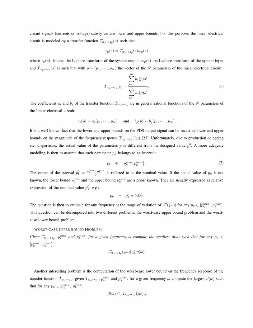
It is a well-known fact that the lower and upper bounds on the PDS output signal can be recast as lower and upper
bounds on the magnitude of the frequency response Twp→zp(jω) [23]. Unfortunately, due to production or ageing
etc. dispersions, the actual value of the parameters p is different from the designed value p0. A more adequate
modeling is then to assume that each parameter pk belongs to an interval:
pk ∈[pmink , pmaxk
]. (2)
The center of the interval p0k =
pmaxk +pmin
k
2 is referred to as the nominal value. If the actual value of pk is not
known, the lower bound pmink and the upper bound pmaxk are a priori known. They are usually expressed as relative
expression of the nominal value p0k, e.g.:
pk = p0k ± 50%.
The question is then to evaluate for any frequency ω the range of variation of |F (jω)| for any pk ∈ [pmink , pmaxk ].
This question can be decomposed into two different problems: the worst-case upper bound problem and the worst-
case lower bound problem.
WORST-CASE UPPER BOUND PROBLEM
Given Twp→zp , pmink and pmaxk , for a given frequency ω compute the smallest η(ω) such that for any pk ∈
[pmink , pmaxk ]
|Twp→zp(jω)| ≤ η(ω).
Another interesting problem is the computation of the worst-case lower bound on the frequency response of the
transfer function Twp→zp : given Twp→zp , pmink and pmaxk , for a given frequency ω compute the largest β(ω) such
that for any pk ∈ [pmink , pmaxk ]
β(ω) ≤ |Twp→zp(jω)|.
Nevertheless in the sequel, we focus on the WORST-CASE UPPER BOUND PROBLEM since the worst-case lower
bound problem can be recast as an equivalent WORST-CASE UPPER BOUND PROBLEM with the upper bound η(jω)
defined as 1β(ω) and the transfer function Twp→zp defined as T−1
wp→zp .
In the case when zp(s) and wp(s) are vectors (with nz = dim(zp) and nw = dim(wp)) i.e. Multi-Input Multi-
Output (MIMO) case, Twp→zp(s) previously defined by (1) is now a matrix of transfer functions. The formulation
of the WORST-CASE UPPER BOUND PROBLEM is extended as follows.
MIMO WORST-CASE UPPER BOUND PROBLEM
Given Twp→zp , pmink and pmaxk , for a given frequency ω compute the smallest η(ω) such that for any pk ∈
[pmink , pmaxk ]
σmax(Twp→zp(jω)
)≤ η(ω).
As in the single input, single output case, another interesting problem is the computation of the worst-case lower
bound on the frequency response of the transfer function Twp→zp : given Twp→zp , pmink and pmaxk , for a given
frequency ω compute the largest β(ω) such that for any pk ∈ [pmink , pmaxk ]
β(ω) ≤ σmin(Twp→zp(jω)
).
Nevertheless, in the sequel and for the same reasons as previously, we focus on the MIMO upper bound case
only. In the next section, we reveal how the MIMO WORST-CASE UPPER BOUND PROBLEM is solved using robust
control approach.
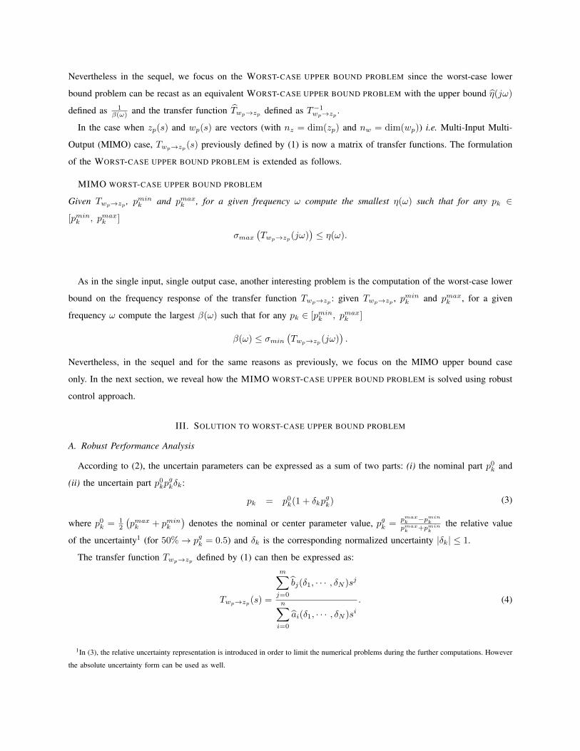
III. SOLUTION TO WORST-CASE UPPER BOUND PROBLEM
A. Robust Performance Analysis
According to (2), the uncertain parameters can be expressed as a sum of two parts: (i) the nominal part p0k and
(ii) the uncertain part p0kpgkδk:
pk = p0k(1 + δkp
gk) (3)
where p0k = 1
2
(pmaxk + pmink
)denotes the nominal or center parameter value, pgk =
pmaxk −pmin
k
pmaxk +pmin
k
the relative value
of the uncertainty1 (for 50%→ pgk = 0.5) and δk is the corresponding normalized uncertainty |δk| ≤ 1.
The transfer function Twp→zp defined by (1) can then be expressed as:
Twp→zp(s) =
m∑j=0
bj(δ1, · · · , δN )sj
n∑i=0
ai(δ1, · · · , δN )si. (4)
1In (3), the relative uncertainty representation is introduced in order to limit the numerical problems during the further computations. However
the absolute uncertainty form can be used as well.
As the coefficients ai(δ1, · · · , δN ) and bj(δ1, · · · , δN ) are rational function of δ1, · · · , δN , zp(s) = Twp→zp(s)wp(s)
can always be transformed as [19]: z (s)
zp (s)
= M (s)
w (s)
wp (s)
and w (s) = ∆ (s) z (s) (5)
where ∆ is defined by
∆ =
δ1In1 0 0
0. . . 0
0 0 δNInN
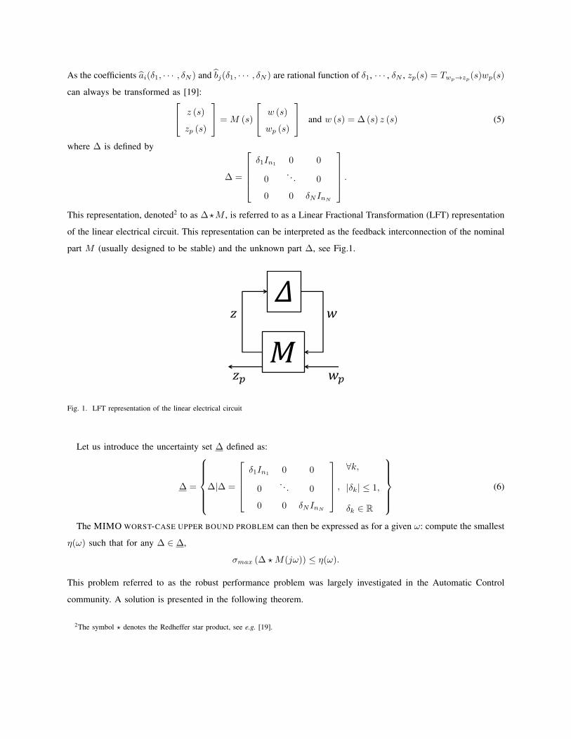
.This representation, denoted2 to as ∆?M , is referred to as a Linear Fractional Transformation (LFT) representation
of the linear electrical circuit. This representation can be interpreted as the feedback interconnection of the nominal
part M (usually designed to be stable) and the unknown part ∆, see Fig.1.
Fig. 1. LFT representation of the linear electrical circuit
Let us introduce the uncertainty set ∆ defined as:
∆ =
∆|∆ =
δ1In1
0 0
0. . . 0
0 0 δNInN
,∀k,
|δk| ≤ 1,
δk ∈ R
(6)
The MIMO WORST-CASE UPPER BOUND PROBLEM can then be expressed as for a given ω: compute the smallest
η(ω) such that for any ∆ ∈ ∆,
σmax (∆ ? M(jω)) ≤ η(ω).
This problem referred to as the robust performance problem was largely investigated in the Automatic Control
community. A solution is presented in the following theorem.
2The symbol ? denotes the Redheffer star product, see e.g. [19].
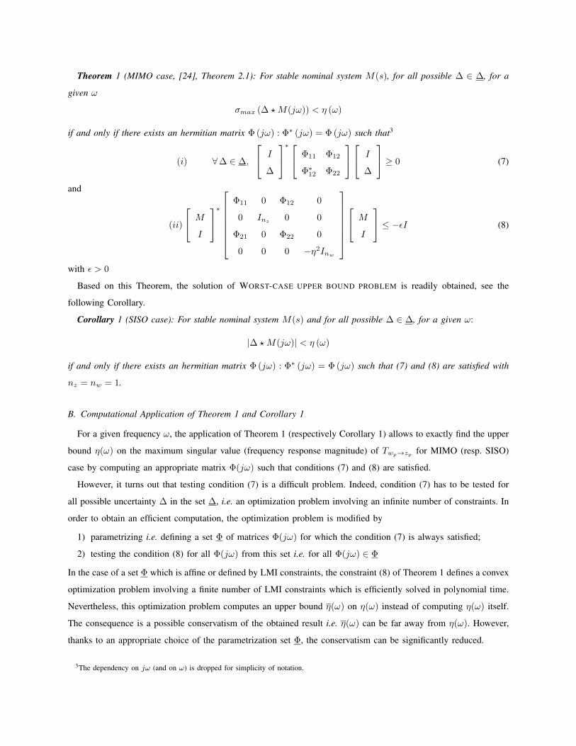
Theorem 1 (MIMO case, [24], Theorem 2.1): For stable nominal system M(s), for all possible ∆ ∈ ∆, for a
given ω
σmax (∆ ? M(jω)) < η (ω)
if and only if there exists an hermitian matrix Φ (jω) : Φ∗ (jω) = Φ (jω) such that3
(i) ∀∆ ∈ ∆,
I
∆
∗ Φ11 Φ12
Φ∗12 Φ22
I
∆
≥ 0 (7)
and
(ii)
M
I
∗
Φ11 0 Φ12 0
0 Inz 0 0
Φ21 0 Φ22 0
0 0 0 −η2Inw
M
I
≤ −εI (8)
with ε > 0
Based on this Theorem, the solution of WORST-CASE UPPER BOUND PROBLEM is readily obtained, see the
following Corollary.
Corollary 1 (SISO case): For stable nominal system M(s) and for all possible ∆ ∈ ∆, for a given ω:
|∆ ? M(jω)| < η (ω)
if and only if there exists an hermitian matrix Φ (jω) : Φ∗ (jω) = Φ (jω) such that (7) and (8) are satisfied with
nz = nw = 1.
B. Computational Application of Theorem 1 and Corollary 1
For a given frequency ω, the application of Theorem 1 (respectively Corollary 1) allows to exactly find the upper
bound η(ω) on the maximum singular value (frequency response magnitude) of Twp→zp for MIMO (resp. SISO)
case by computing an appropriate matrix Φ(jω) such that conditions (7) and (8) are satisfied.
However, it turns out that testing condition (7) is a difficult problem. Indeed, condition (7) has to be tested for
all possible uncertainty ∆ in the set ∆, i.e. an optimization problem involving an infinite number of constraints. In
order to obtain an efficient computation, the optimization problem is modified by
1) parametrizing i.e. defining a set Φ of matrices Φ(jω) for which the condition (7) is always satisfied;
2) testing the condition (8) for all Φ(jω) from this set i.e. for all Φ(jω) ∈ Φ
In the case of a set Φ which is affine or defined by LMI constraints, the constraint (8) of Theorem 1 defines a convex
optimization problem involving a finite number of LMI constraints which is efficiently solved in polynomial time.
Nevertheless, this optimization problem computes an upper bound η(ω) on η(ω) instead of computing η(ω) itself.
The consequence is a possible conservatism of the obtained result i.e. η(ω) can be far away from η(ω). However,
thanks to an appropriate choice of the parametrization set Φ, the conservatism can be significantly reduced.
3The dependency on jω (and on ω) is dropped for simplicity of notation.
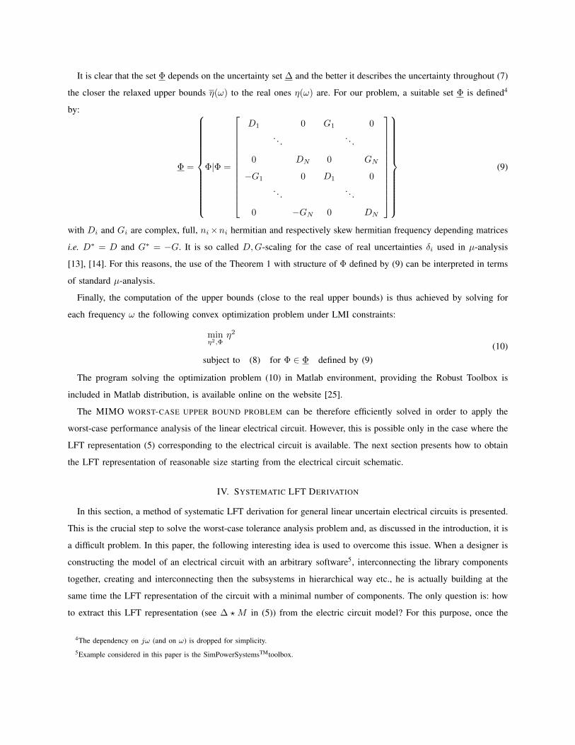
It is clear that the set Φ depends on the uncertainty set ∆ and the better it describes the uncertainty throughout (7)
the closer the relaxed upper bounds η(ω) to the real ones η(ω) are. For our problem, a suitable set Φ is defined4
by:
Φ =
Φ|Φ =
D1 0 G1 0
. . . . . .
0 DN 0 GN
−G1 0 D1 0
. . . . . .
0 −GN 0 DN
(9)
with Di and Gi are complex, full, ni×ni hermitian and respectively skew hermitian frequency depending matrices
i.e. D∗ = D and G∗ = −G. It is so called D,G-scaling for the case of real uncertainties δi used in µ-analysis
[13], [14]. For this reasons, the use of the Theorem 1 with structure of Φ defined by (9) can be interpreted in terms
of standard µ-analysis.
Finally, the computation of the upper bounds (close to the real upper bounds) is thus achieved by solving for
each frequency ω the following convex optimization problem under LMI constraints:
minη2,Φ
η2
subject to (8) for Φ ∈ Φ defined by (9)(10)
The program solving the optimization problem (10) in Matlab environment, providing the Robust Toolbox is
included in Matlab distribution, is available online on the website [25].
The MIMO WORST-CASE UPPER BOUND PROBLEM can be therefore efficiently solved in order to apply the
worst-case performance analysis of the linear electrical circuit. However, this is possible only in the case where the
LFT representation (5) corresponding to the electrical circuit is available. The next section presents how to obtain
the LFT representation of reasonable size starting from the electrical circuit schematic.
IV. SYSTEMATIC LFT DERIVATION
In this section, a method of systematic LFT derivation for general linear uncertain electrical circuits is presented.
This is the crucial step to solve the worst-case tolerance analysis problem and, as discussed in the introduction, it is
a difficult problem. In this paper, the following interesting idea is used to overcome this issue. When a designer is
constructing the model of an electrical circuit with an arbitrary software5, interconnecting the library components
together, creating and interconnecting then the subsystems in hierarchical way etc., he is actually building at the
same time the LFT representation of the circuit with a minimal number of components. The only question is: how
to extract this LFT representation (see ∆ ? M in (5)) from the electric circuit model? For this purpose, once the
4The dependency on jω (and on ω) is dropped for simplicity.5Example considered in this paper is the SimPowerSystemsTMtoolbox.
electric circuit model is built, first the traditionally used component models (such as resistor, capacitor, inductor
models etc.) are replaced by uncertain component models proposed in this section. The number and ordering of
these uncertain components automatically defines the structure of the block ∆. Then, the extraction procedure is
performed in order to obtain the matrix transfer function M(s).
In the following subsection, a library of elementary uncertain linear electric circuit components is proposed.
Since these uncertain components are very similar to the standard ones, there is only the need of regular electrical
engineer’s knowledge to use (and build) the uncertain model. It is even possible to combine the regular and uncertain
components in order to avoid time consuming computation in the case where some uncertainties can be neglected.
Then, in next subsection, the procedure of LFT representation extraction is presented.
A. Block Diagram of Uncertain Electrical Components
The detailed description of uncertain components is given only for Resistor, Capacitor and Mutual Inductor while
other components can be deduced in a similar fashion. A more complete table (or library) of uncertain components
is then presented.
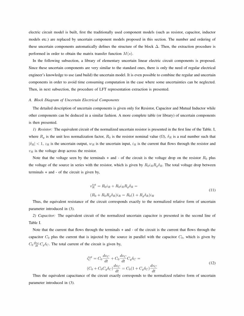
1) Resistor: The equivalent circuit of the normalized uncertain resistor is presented in the first line of the Table. I,
where Rg is the unit less normalization factor, R0 is the resistor nominal value (Ω), δR is a real number such that
|δR| < 1, zR is the uncertain output, wR is the uncertain input, iR is the current that flows through the resistor and
vR is the voltage drop across the resistor.
Note that the voltage seen by the terminals + and - of the circuit is the voltage drop on the resistor R0 plus
the voltage of the source in series with the resistor, which is given by R0iRRgδR. The total voltage drop between
terminals + and - of the circuit is given by,
vtotR = R0iR +R0iRRgδR =
(R0 +R0RgδR)iR = R0(1 +RgδR)iR
(11)
Thus, the equivalent resistance of the circuit corresponds exactly to the normalized relative form of uncertain
parameter introduced in (3).
2) Capacitor: The equivalent circuit of the normalized uncertain capacitor is presented in the second line of
Table I.
Note that the current that flows through the terminals + and - of the circuit is the current that flows through the
capacitor C0 plus the current that is injected by the source in parallel with the capacitor C0, which is given by
C0dvCdt CgδC . The total current of the circuit is given by,
itotC = C0dvCdt
+ C0dvCdt
CgδC =
(C0 + C0CgδC)dvCdt
= C0(1 + CgδC)dvCdt
(12)
Thus the equivalent capacitance of the circuit exactly corresponds to the normalized relative form of uncertain
parameter introduced in (3).
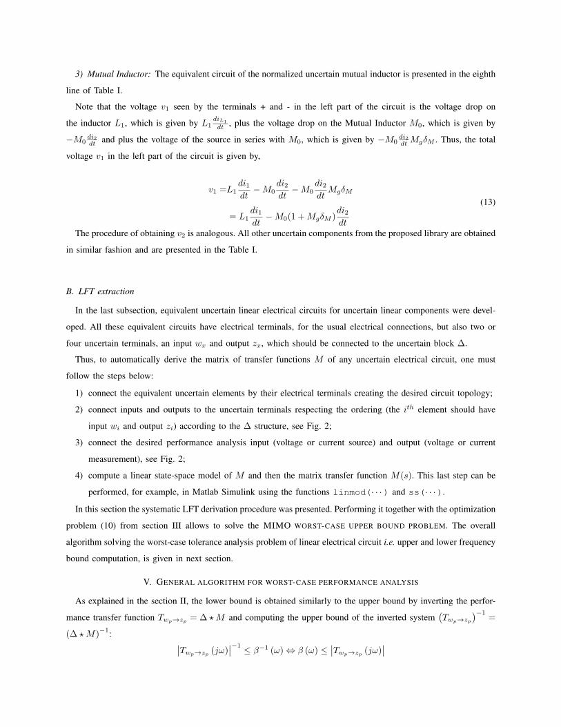
3) Mutual Inductor: The equivalent circuit of the normalized uncertain mutual inductor is presented in the eighth
line of Table I.
Note that the voltage v1 seen by the terminals + and - in the left part of the circuit is the voltage drop on
the inductor L1, which is given by L1diL1
dt , plus the voltage drop on the Mutual Inductor M0, which is given by
−M0di2dt and plus the voltage of the source in series with M0, which is given by −M0
di2dt MgδM . Thus, the total
voltage v1 in the left part of the circuit is given by,
v1 =L1di1dt−M0
di2dt−M0
di2dtMgδM
= L1di1dt−M0(1 +MgδM )
di2dt
(13)
The procedure of obtaining v2 is analogous. All other uncertain components from the proposed library are obtained
in similar fashion and are presented in the Table I.
B. LFT extraction
In the last subsection, equivalent uncertain linear electrical circuits for uncertain linear components were devel-
oped. All these equivalent circuits have electrical terminals, for the usual electrical connections, but also two or
four uncertain terminals, an input wx and output zx, which should be connected to the uncertain block ∆.
Thus, to automatically derive the matrix of transfer functions M of any uncertain electrical circuit, one must
follow the steps below:
1) connect the equivalent uncertain elements by their electrical terminals creating the desired circuit topology;
2) connect inputs and outputs to the uncertain terminals respecting the ordering (the ith element should have
input wi and output zi) according to the ∆ structure, see Fig. 2;
3) connect the desired performance analysis input (voltage or current source) and output (voltage or current
measurement), see Fig. 2;
4) compute a linear state-space model of M and then the matrix transfer function M(s). This last step can be
performed, for example, in Matlab Simulink using the functions linmod(· · ·) and ss(· · ·).
In this section the systematic LFT derivation procedure was presented. Performing it together with the optimization
problem (10) from section III allows to solve the MIMO WORST-CASE UPPER BOUND PROBLEM. The overall
algorithm solving the worst-case tolerance analysis problem of linear electrical circuit i.e. upper and lower frequency
bound computation, is given in next section.
V. GENERAL ALGORITHM FOR WORST-CASE PERFORMANCE ANALYSIS
As explained in the section II, the lower bound is obtained similarly to the upper bound by inverting the perfor-
mance transfer function Twp→zp = ∆ ?M and computing the upper bound of the inverted system(Twp→zp
)−1=
(∆ ? M)−1: ∣∣Twp→zp (jω)
∣∣−1 ≤ β−1 (ω)⇔ β (ω) ≤∣∣Twp→zp (jω)
∣∣
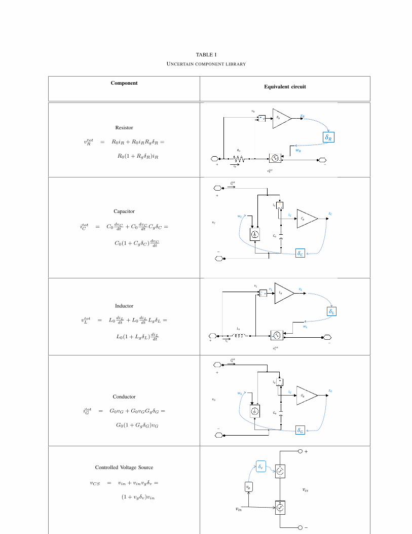
TABLE I
UNCERTAIN COMPONENT LIBRARY
ComponentEquivalent circuit
Resistor
vtotR = R0iR +R0iRRgδR =
R0(1 +RgδR)iR
𝑅0
+ − 𝑖𝑅
𝑣𝑅𝑡𝑜𝑡
𝑅𝑔
𝑣𝑅
𝑧𝑅
𝛿𝑅
𝑤𝑅
Capacitor
itotC = C0dvCdt
+ C0dvCdt
CgδC =
C0(1 + CgδC) dvCdt
𝐶0
𝑣𝐶
+
−
𝑖𝐶𝑡𝑜𝑡
𝑖𝐶
𝐶𝑔 𝑖𝐶
𝛿𝐶
𝑧𝐶 𝑤𝐶
Inductor
vtotL = L0diLdt
+ L0diLdtLgδL =
L0(1 + LgδL)diLdt
𝑣𝐿𝑡𝑜𝑡
+ −
𝑖𝐿
𝐿𝑔
𝑣𝐿 𝑣𝐿 𝑧𝐿
𝛿𝐿
𝑤𝐿 𝐿0
Conductor
itotG = G0vG +G0vGGgδG =
G0(1 +GgδG)vG
𝐺0
𝑣𝐺
+
−
𝑖𝐺𝑡𝑜𝑡
𝑖𝐺
𝐺𝑔 𝑖𝐶
𝛿𝐺
𝑧𝐺 𝑤𝐺
Controlled Voltage Source
vCS = vin + vinvgδv =
(1 + vgδv)vin
𝑣𝑔
𝛿𝑣
𝑣𝑖𝑛
+
−
𝑣𝑐𝑠
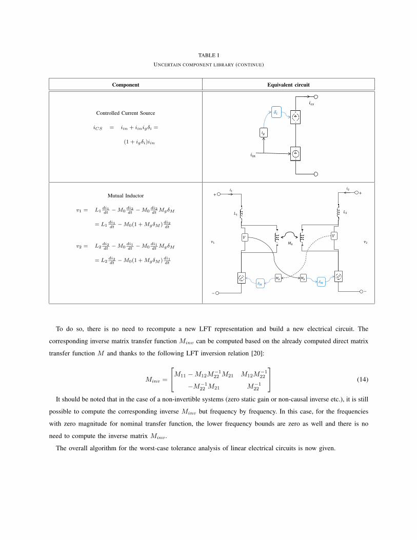
TABLE I
UNCERTAIN COMPONENT LIBRARY (CONTINUE)
Component Equivalent circuit
Controlled Current Source
iCS = iin + iinigδi =
(1 + igδi)iin
𝑖𝑔
𝛿𝑖
𝑖𝑖𝑛
𝑖𝑐𝑠
Mutual Inductor
v1 = L1di1dt−M0
di2dt−M0
di2dtMgδM
= L1di1dt−M0(1 +MgδM ) di2
dt
v2 = L2di2dt−M0
di1dt−M0
di1dtMgδM
= L2di2dt−M0(1 +MgδM ) di1
dt
𝐿1
𝑀0
𝑉
𝛿𝑀
𝑀𝑔
𝑣1
+
−
𝑖1
𝐿2
𝑉
𝛿𝑀 𝑀𝑔
𝑣2
+
−
𝑖2
To do so, there is no need to recompute a new LFT representation and build a new electrical circuit. The
corresponding inverse matrix transfer function Minv can be computed based on the already computed direct matrix
transfer function M and thanks to the following LFT inversion relation [20]:
Minv =
M11 −M12M−122 M21 M12M
−122
−M−122 M21 M−1
22
(14)
It should be noted that in the case of a non-invertible systems (zero static gain or non-causal inverse etc.), it is still
possible to compute the corresponding inverse Minv but frequency by frequency. In this case, for the frequencies
with zero magnitude for nominal transfer function, the lower frequency bounds are zero as well and there is no
need to compute the inverse matrix Minv .
The overall algorithm for the worst-case tolerance analysis of linear electrical circuits is now given.
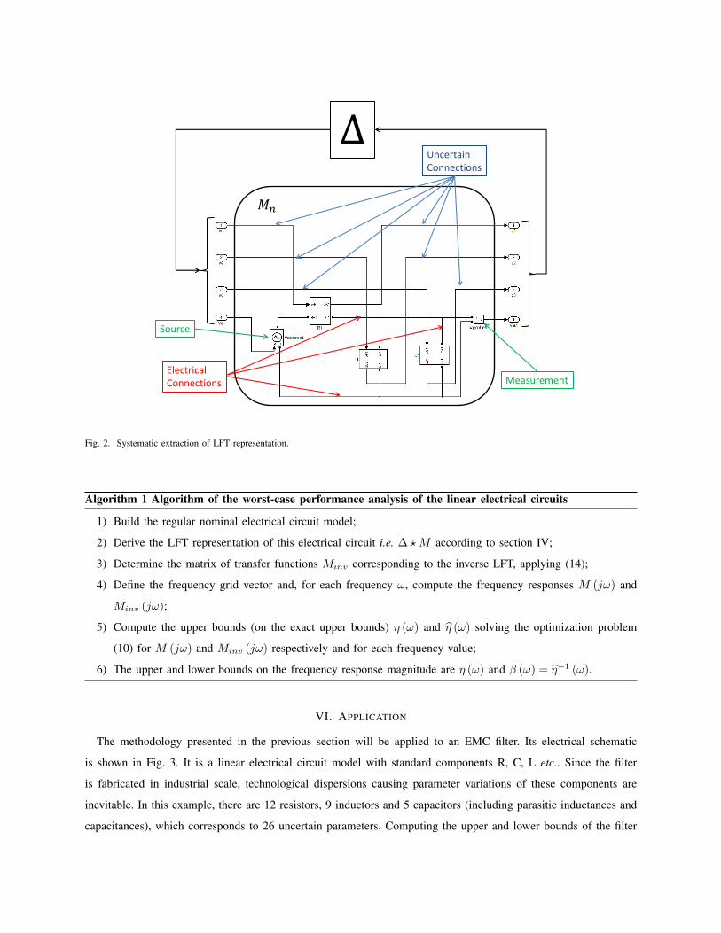
∆
𝑀𝑛
Uncertain Connections
Electrical Connections
Source
Measurement
Fig. 2. Systematic extraction of LFT representation.
Algorithm 1 Algorithm of the worst-case performance analysis of the linear electrical circuits
1) Build the regular nominal electrical circuit model;
2) Derive the LFT representation of this electrical circuit i.e. ∆ ? M according to section IV;
3) Determine the matrix of transfer functions Minv corresponding to the inverse LFT, applying (14);
4) Define the frequency grid vector and, for each frequency ω, compute the frequency responses M (jω) and
Minv (jω);
5) Compute the upper bounds (on the exact upper bounds) η (ω) and η (ω) solving the optimization problem
(10) for M (jω) and Minv (jω) respectively and for each frequency value;
6) The upper and lower bounds on the frequency response magnitude are η (ω) and β (ω) = η−1 (ω).
VI. APPLICATION
The methodology presented in the previous section will be applied to an EMC filter. Its electrical schematic
is shown in Fig. 3. It is a linear electrical circuit model with standard components R, C, L etc.. Since the filter
is fabricated in industrial scale, technological dispersions causing parameter variations of these components are
inevitable. In this example, there are 12 resistors, 9 inductors and 5 capacitors (including parasitic inductances and
capacitances), which corresponds to 26 uncertain parameters. Computing the upper and lower bounds of the filter
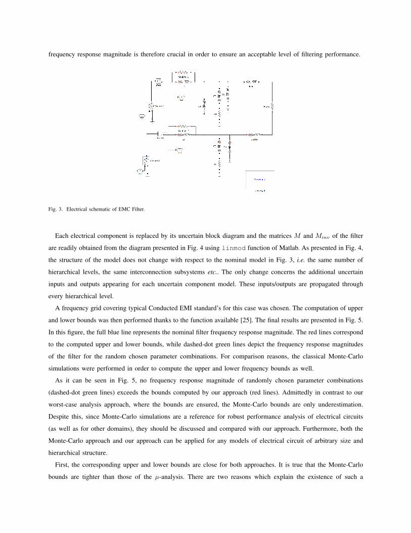
frequency response magnitude is therefore crucial in order to ensure an acceptable level of filtering performance.
Fig. 3. Electrical schematic of EMC Filter.
Each electrical component is replaced by its uncertain block diagram and the matrices M and Minv of the filter
are readily obtained from the diagram presented in Fig. 4 using linmod function of Matlab. As presented in Fig. 4,
the structure of the model does not change with respect to the nominal model in Fig. 3, i.e. the same number of
hierarchical levels, the same interconnection subsystems etc.. The only change concerns the additional uncertain
inputs and outputs appearing for each uncertain component model. These inputs/outputs are propagated through
every hierarchical level.
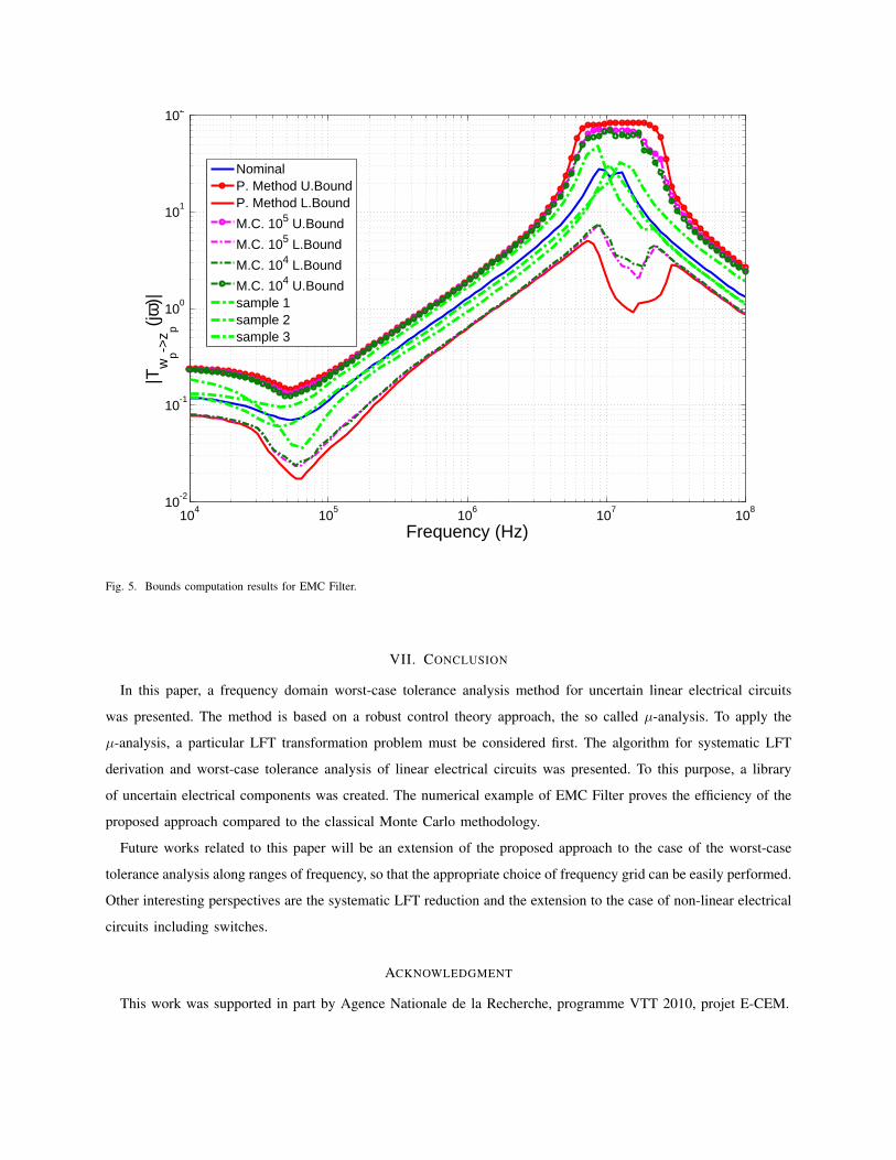
A frequency grid covering typical Conducted EMI standard’s for this case was chosen. The computation of upper
and lower bounds was then performed thanks to the function available [25]. The final results are presented in Fig. 5.
In this figure, the full blue line represents the nominal filter frequency response magnitude. The red lines correspond
to the computed upper and lower bounds, while dashed-dot green lines depict the frequency response magnitudes
of the filter for the random chosen parameter combinations. For comparison reasons, the classical Monte-Carlo
simulations were performed in order to compute the upper and lower frequency bounds as well.
As it can be seen in Fig. 5, no frequency response magnitude of randomly chosen parameter combinations
(dashed-dot green lines) exceeds the bounds computed by our approach (red lines). Admittedly in contrast to our
worst-case analysis approach, where the bounds are ensured, the Monte-Carlo bounds are only underestimation.
Despite this, since Monte-Carlo simulations are a reference for robust performance analysis of electrical circuits
(as well as for other domains), they should be discussed and compared with our approach. Furthermore, both the
Monte-Carlo approach and our approach can be applied for any models of electrical circuit of arbitrary size and
hierarchical structure.
First, the corresponding upper and lower bounds are close for both approaches. It is true that the Monte-Carlo
bounds are tighter than those of the µ-analysis. There are two reasons which explain the existence of such a
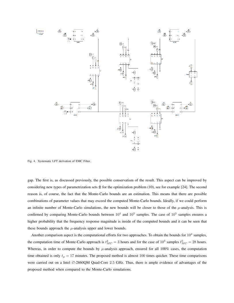
Fig. 4. Systematic LFT derivation of EMC Filter.
gap. The first is, as discussed previously, the possible conservatism of the result. This aspect can be improved by
considering new types of parametrization sets Φ for the optimization problem (10), see for example [24]. The second
reason is, of course, the fact that the Monte-Carlo bounds are an estimation. This means that there are possible
combinations of parameter values that may exceed the computed Monte-Carlo bounds. Ideally, if we could perform
an infinite number of Monte-Carlo simulations, the new bounds will be closer to those of the µ-analysis. This is
confirmed by comparing Monte-Carlo bounds between 104 and 105 samples. The case of 105 samples ensures a
higher probability that the frequency response magnitude is inside of the computed bounds and it can be seen that
these bounds approach the µ-analysis upper and lower bounds.
Another comparison aspect is the computational efforts for two approaches. To obtain the bounds for 104 samples,
the computation time of Monte-Carlo approach is t4MC = 3 hours and for the case of 105 samples t5MC = 28 hours.
Whereas, in order to compute the bounds by µ-analysis approach, ensured for all 100% cases, the computation
time obtained is only tµ = 17 minutes. The proposed method is almost 100 times quicker. These time comparisons
were carried out on a Intel i7-2860QM Quad-Core 2.5 GHz. Thus, there is ample evidence of advantages of the
proposed method when compared to the Monte-Carlo simulations.
104
105
106
107
108
10-2
10-1
100
101
102
Frequency (Hz)
|Tw
p->z p(jω
)|
NominalP. Method U.BoundP. Method L.Bound
M.C. 105 U.Bound
M.C. 105 L.Bound
M.C. 104 L.Bound
M.C. 104 U.Boundsample 1sample 2sample 3
Fig. 5. Bounds computation results for EMC Filter.
VII. CONCLUSION
In this paper, a frequency domain worst-case tolerance analysis method for uncertain linear electrical circuits
was presented. The method is based on a robust control theory approach, the so called µ-analysis. To apply the
µ-analysis, a particular LFT transformation problem must be considered first. The algorithm for systematic LFT
derivation and worst-case tolerance analysis of linear electrical circuits was presented. To this purpose, a library
of uncertain electrical components was created. The numerical example of EMC Filter proves the efficiency of the
proposed approach compared to the classical Monte Carlo methodology.
Future works related to this paper will be an extension of the proposed approach to the case of the worst-case
tolerance analysis along ranges of frequency, so that the appropriate choice of frequency grid can be easily performed.
Other interesting perspectives are the systematic LFT reduction and the extension to the case of non-linear electrical
circuits including switches.
ACKNOWLEDGMENT
This work was supported in part by Agence Nationale de la Recherche, programme VTT 2010, projet E-CEM.
REFERENCES
[1] S. J. Julier, Jeffrey, and K. Uhlmann, “Unscented filtering and nonlinear estimation,” in Proceedings of the IEEE, 2004, pp. 401–422.
[2] L. de Menezes, A. Ajayi, C. Christopoulos, P. Sewell, and G. Borges, “Efficient computation of stochastic electromagnetic problems using
unscented transforms,” Science, Measurement Technology, IET, vol. 2, no. 2, pp. 88 –95, march 2008.
[3] H. Kettani and B. Barmish, “A new monte carlo circuit simulation paradigm with specific results for resistive networks,” Circuits and
Systems I: Regular Papers, IEEE Transactions on, vol. 53, no. 6, pp. 1289 –1299, june 2006.
[4] M. Ferber De Vieira Lessa, C. Vollaire, L. Krahenbuhl, and A. Vasconcelos, Joao, “Adaptive unscented transform for uncertainty
quantification in EMC large-scale systems,” in Proc. of the 12th International Workshop on Optimization and Inverse Problems in
Electromagnetism, Ghent, Belgium, Sep. 2012, p. CD.
[5] M. Ferber, C. Vollaire, L. Krahenbuhl, J.-L. Coulomb, and J. A. Vasconcelos, “Conducted EMI of DC–DC converters with parametric
uncertainties,” Electromagnetic Compatibility, IEEE Transactions on, vol. PP, no. 99, pp. 1 –8, 2013.
[6] S. Skelboe, “True worst-case analysis of linear electrical circuits by interval arithmetic,” Circuits and Systems, IEEE Transactions on,
vol. 26, no. 10, pp. 874–879, Oct 1979.
[7] W. Tian, X.-T. Ling, and R. Liu, “Novel methods for circuit worst-case tolerance analysis,” Circuits and Systems I: Fundamental Theory
and Applications, IEEE Transactions on, vol. 43, no. 4, pp. 272–278, Apr 1996.
[8] M. Tian and C. J. R. Shi, “Worst case tolerance analysis of linear analog circuits using sensitivity bands,” Circuits and Systems I:
Fundamental Theory and Applications, IEEE Transactions on, vol. 47, no. 8, pp. 1138–1145, Aug 2000.
[9] N. Femia and G. Spagnuolo, “True worst-case circuit tolerance analysis using genetic algorithms and affine arithmetic,” Circuits and
Systems I: Fundamental Theory and Applications, IEEE Transactions on, vol. 47, no. 9, pp. 1285–1296, Sep 2000.
[10] J. Leyva-Ramos and J. Morales-Saldana, “Uncertainty models for switch-mode DC-DC converters,” Circuits and Systems I: Fundamental
Theory and Applications, IEEE Transactions on, vol. 47, no. 2, pp. 200–203, Feb 2000.
[11] R. D. Braatz, P. M. Young, J. C. Doyle, and M. Morari, “Computational complexity of µ calculation,” IEEE Trans. Aut. Control, vol.
AC-39, no. 5, pp. 1000–1002, May 1994.
[12] L. Kolev, “Worst-case tolerance analysis of linear DC and AC electric circuits,” Circuits and Systems I: Fundamental Theory and
Applications, IEEE Transactions on, vol. 49, no. 12, pp. 1693–1701, Dec 2002.
[13] J. Doyle, “Analysis of feedback systems with structured uncertainties,” IEE Proc., vol. 129-D, no. 6, pp. 242–250, Nov. 1982.
[14] M. K. H. Fan, A. L. Tits, and J. C. Doyle, “Robustness in the presence of mixed parametric uncertainty and unmodeled dynamics,” IEEE
Trans. Aut. Control, vol. 36, no. 1, pp. 25–38, Jan 1991.
[15] S. Skogestad and I. Postlethwaite, Multivariable Feedback Control, Analysis and Design. John Wiley and Sons Chischester, 2005.
[16] Y. Nesterov, Introductory Lectures on Convex Optimization, ser. Applied optimization. Boston/Dordrecht/London: Kluxer Academic
Publishers, 2004, no. 87.
[17] R. Tymerski, “Worst-case stability analysis of switching regulators using the structured singular value,” Power Electronics, IEEE
Transactions on, vol. 11, no. 5, pp. 723–730, Sep 1996.
[18] J. Wang, O. Hafiz, and J. Li, “A linear fractional transform (LFT) based model for interconnect parametric uncertainty,” in Design
Automation Conference, 2004. Proceedings. 41st, July 2004, pp. 375–380.
[19] K. Zhou, J. Doyle, and K. Glover, Robust and Optimal Control. Prentice Hall, New Jersey, 1995.
[20] J. Doyle, A. Packard, and K. Zhou, “Review of LFTs, LMIs, and µ,” in Decision and Control, 1991., Proceedings of the 30th IEEE
Conference on, Dec 1991, pp. 1227–1232 vol.2.
[21] S. Font, “Methodologie pour prendre en compte la robustesse des systemes asservis: optimisation H∞ et approche symbolique de la forme
standard,” Ph.D. dissertation, Universite Paris XI Orsay, France, 1995.
[22] R. A. Horn and C. A. Johnson, Matrix Analysis. Cambridge University Press, 1985.
[23] R. Ozenbaugh and T. Pullen, EMI Filter Design – 3rd ed, ser. Electrical and computer engineering. CRC Press – Taylor & Francis, 2012.
[24] G. Scorletti, X. Bombois, M. Barenthin, and V. Fromion, “Improved efficient analysis for systems with uncertain parameters,” in IEEE
Conf. Decision and Control, New Orleans, dec. 2007, pp. 5038–5043.
[25] [Online]. Available: https://sites.google.com/site/fastwctanalysis/