Szabolcs Berezvai

Final Project

Budapest University of Technology and Economics

Faculty of Mechanical Engineering

Department of Applied Mechanics

Final Projects

Budapest University of Technology and Economics

Faculty of Mechanical Engineering

Department of Applied Mechanics

Szabolcs BEREZVAI

Visco-hyperelastic characterization ofpolymeric foams

Final Project

Supervisor: Dr. Attila KOSSA, assistant professor

Department of Applied Mechanics

Budapest, 2015

Copyright c© Szabolcs Berezvai, 2015

Declarations

Declaration of acceptance

This thesis fulfils all formal and content requirements prescribed by the Faculty of MechanicalEngineering of Budapest University of Technology and Economics, as well as it fully complies alltasks specified in the transcript. I consider this thesis as it is suitable for submission for publicreview and for public presentation.

Done at Budapest, 11.12.2015

dr. Attila Kossa

Declaration of independent work

I, Szabolcs Berezvai, the undersigned, hereby declare that the present thesis work has beenprepared by myself without any unauthorized help or assistance such that only the specifiedsources (references, tools, etc.) were used. All parts taken from other sources word by word orafter rephrasing but with identical meaning were unambiguously identified with explicit referenceto the sources utilized.

Szabolcs Berezvai

Declaration of authorization

I authorize the Faculty of Mechanical Engineering of the Budapest University of Technologyand Economics to publish the principal data of the thesis work (author’s name, title, abstracts inEnglish and in Hungarian, year of preparation, supervisor’s name, etc.) in a searchable, public,electronic and online database and to publish the full text of the thesis work on the internalnetwork of the university (or for authenticated users). I declare that the submitted hard copy ofthe thesis work and its electronic version are identical. Full text of thesis works classified uponthe decision of the Dean will be published after two years.

Done at Budapest, 11.12.2015

Szabolcs Berezvai

vii

Acknowledgements

First of all, I would like to express my deepest thanks to my supervisor, dr. Attila KOSSA assistantprofessor (Department of Applied Mechanics) for his outstanding guidance and constant supportduring my work. I am indebted for all the invaluable support and inspiration he gave me duringour common work in the last years. I am also grateful that he endeared to me the mechanics ofpolymer foams and introduced me the beauty of researchers’ life.

I got insights into the manufacturing technology of polyer foams during my summer internshipat Furukawa Electric Institute of Technology (FETI Kft). These experiences were beneficial formy thesis.

I would like to thank my friends, mates and my family, who I could always count on indeed.Especially to my Mum, who always supported my dreams and goals.

This research has been supported by the Hungarian Scientific Research Fund, Hungary (ProjectIdentifier: PD 108691) and the National Talent Programme of the Hungarian Government (Con-tract Identifier: NTP-EF-P-15-0085), which are gratefully acknowledged.

ix

AbstractKeywords: viscoelasticity, hyperelasticity, parameter fitting, finite strain theory, polymer foams

Polymer foams are widely applied cellular materials due to their mechanical behaviour andhigh energy absorption properties. The deformations of polymer foams can be characterised bylarge strains (in case of volumetric compression) and large displacements, which shows visco-elasticmaterial behaviour. The main field of application is packaging and impact protection, but polymerfoams appear in everyday use like as ear-plugs and memory foams as well.

The behaviour of large elastic and viscoelastic materials can be described by the so-called visco-hyperelastic material model, which combines the hyperelastic and the viscoelastic material models.In this approach the time-dependent stress-relaxation phenomenon is modelled using Prony-seriesrepresentation, while for the long-term time-independent behaviour hyperelastic material modelis proposed, which can be derived from the corresponding strain energy function.

In this thesis I investigate the modelling of the visco-hyperelastic material behaviour in case ofhomogeneous deformations of a particular memory foam material applied in mattresses. The mostwidely used compressible hyperelastic material model, the Ogden-Hill model and the finite strainviscoelastic constitutive law implemented in the commercial finite element software ABAQUS arealso provided. Using these models the closed-form stress response functions were determined incase of homogeneous deformations. This provided closed-form solutions, which are not availablein the literature yet, enables us to obtain material parameters directly from the experimental datausing parameter-fitting.

The usual algorithm of parameter-fitting is to separate the parameter-fitting of the long-termbehaviour and the parameter-fitting of the stress relaxation. In this approach it is assumed thatthe stress-relaxation is investigated in case of step load. However, in case of real measurements onlyramp loading can be performed, which leads to errors in the relaxation test data. The analyticallydetermined stress response yields that the entire visco-hyperelastic model can be fitted to thereal measurement data in case of ramp test. Using this latter method more accurate materialparameters can be provided for the investigated memory foam material. Finally, the fitted modelwas investigated in Abaqus in order to analyse the numerical behaviour of the model and tocompare it with the measured data.

xi

Contents

1 Introduction 1

1.1 Polymer foams and their application . . . . . . . . . . . . . . . . . . . . . . . . . 11.2 Aim of the work . . . . . . . . . . . . . . . . . . . . . . . . . . . . . . . . . . . . . 21.3 Outline of the thesis . . . . . . . . . . . . . . . . . . . . . . . . . . . . . . . . . . 41.4 Nomenclature . . . . . . . . . . . . . . . . . . . . . . . . . . . . . . . . . . . . . . 5

2 Hyperelastic modelling of polymer foams 7

2.1 Theory of hyperelastic constitutive equations . . . . . . . . . . . . . . . . . . . . . 72.2 Ogden–Hill’s hyperelastic model . . . . . . . . . . . . . . . . . . . . . . . . . . . . 10

2.2.1 The history of the Ogden–Hill’s hyperelastic model . . . . . . . . . . . . . 112.2.2 Stress solutions . . . . . . . . . . . . . . . . . . . . . . . . . . . . . . . . . 12

2.3 Material stability . . . . . . . . . . . . . . . . . . . . . . . . . . . . . . . . . . . . 12

3 Viscoelastic material modelling 15

3.1 Viscoelastic material behaviour . . . . . . . . . . . . . . . . . . . . . . . . . . . . 153.1.1 The mechanical model of relaxation in 1D . . . . . . . . . . . . . . . . . . 163.1.2 The stress solution for 1D loading . . . . . . . . . . . . . . . . . . . . . . . 17

3.2 Finite strain viscoelasticity . . . . . . . . . . . . . . . . . . . . . . . . . . . . . . . 183.3 Numerical implementation . . . . . . . . . . . . . . . . . . . . . . . . . . . . . . . 20

4 Closed-form stress solutions 21

4.1 Homogeneous deformations . . . . . . . . . . . . . . . . . . . . . . . . . . . . . . . 214.1.1 Uniaxial compression . . . . . . . . . . . . . . . . . . . . . . . . . . . . . . 224.1.2 Equibiaxial compression . . . . . . . . . . . . . . . . . . . . . . . . . . . . 234.1.3 Volumetric compression . . . . . . . . . . . . . . . . . . . . . . . . . . . . 244.1.4 Simple shear . . . . . . . . . . . . . . . . . . . . . . . . . . . . . . . . . . . 25

4.2 Solution of the hereditary integral . . . . . . . . . . . . . . . . . . . . . . . . . . . 264.2.1 Uploading part . . . . . . . . . . . . . . . . . . . . . . . . . . . . . . . . . 284.2.2 Relaxation part . . . . . . . . . . . . . . . . . . . . . . . . . . . . . . . . . 284.2.3 Summary . . . . . . . . . . . . . . . . . . . . . . . . . . . . . . . . . . . . 29

5 Measurements 31

5.1 Introduction . . . . . . . . . . . . . . . . . . . . . . . . . . . . . . . . . . . . . . . 315.1.1 Specimens . . . . . . . . . . . . . . . . . . . . . . . . . . . . . . . . . . . . 325.1.2 Evaluation of measurements . . . . . . . . . . . . . . . . . . . . . . . . . . 33

5.2 Relaxation test . . . . . . . . . . . . . . . . . . . . . . . . . . . . . . . . . . . . . 345.2.1 Results . . . . . . . . . . . . . . . . . . . . . . . . . . . . . . . . . . . . . 34

5.3 Cyclic test . . . . . . . . . . . . . . . . . . . . . . . . . . . . . . . . . . . . . . . . 365.3.1 Results . . . . . . . . . . . . . . . . . . . . . . . . . . . . . . . . . . . . . . 37

5.4 Summary of the measurement results . . . . . . . . . . . . . . . . . . . . . . . . . 38

xiii

CONTENTS

6 Parameter fitting 39

6.1 The method of parameter fitting . . . . . . . . . . . . . . . . . . . . . . . . . . . . 396.2 Parameter fitting algorithms in case of visco-hyperelastic materials . . . . . . . . . 406.3 Separated fitting of parameters . . . . . . . . . . . . . . . . . . . . . . . . . . . . 41

6.3.1 Hyperelastic parameters . . . . . . . . . . . . . . . . . . . . . . . . . . . . 416.3.2 Prony parameters . . . . . . . . . . . . . . . . . . . . . . . . . . . . . . . . 436.3.3 Validation with FEA . . . . . . . . . . . . . . . . . . . . . . . . . . . . . . 446.3.4 The results of the separated fitting . . . . . . . . . . . . . . . . . . . . . . 45

6.4 Closed-form parameter fitting . . . . . . . . . . . . . . . . . . . . . . . . . . . . . 466.4.1 Identification of material parameters . . . . . . . . . . . . . . . . . . . . . 466.4.2 Predictions on the material behaviour . . . . . . . . . . . . . . . . . . . . . 48

6.5 Evaluation of results . . . . . . . . . . . . . . . . . . . . . . . . . . . . . . . . . . 50

7 Summary of results 53

7.1 Summary in English . . . . . . . . . . . . . . . . . . . . . . . . . . . . . . . . . . 537.2 Summary in Hungarian - Az eredmenyek osszefoglalasa . . . . . . . . . . . . . . . 55

Appendices 57

A Relation of the Hyperfoam material model and the Hooke’s law 59

B Numerical implementation of visco-hyperelastic model 61

B.1 Integration of the hydrostatic stress . . . . . . . . . . . . . . . . . . . . . . . . . . 61B.2 Integration of the deviatoric stress . . . . . . . . . . . . . . . . . . . . . . . . . . . 62B.3 Total stress solution . . . . . . . . . . . . . . . . . . . . . . . . . . . . . . . . . . 63

C The incomplete gamma function 65

C.1 The (complete) gamma function . . . . . . . . . . . . . . . . . . . . . . . . . . . . 65C.2 The upper incomplete gamma function . . . . . . . . . . . . . . . . . . . . . . . . 66C.3 Special cases . . . . . . . . . . . . . . . . . . . . . . . . . . . . . . . . . . . . . . . 66

References 68

xiv

1Introduction

1.1 Polymer foams and their application

Polymer foams are widely applied cellular materials, thanks to their favourable mechanical be-

haviour and high energy absorption properties. Due to their cellular structure, polymer foams are

light-weight with low overall density since they are typically 90% space. Additionally, the me-

chanical behaviour is characterised by low moduli, such as the elastic modulus, the shear modulus

and the bulk modulus. The deformation of polymer foams also exhibits large deformations and

displacements. These properties might suggest that polymer foams are of little use from the indus-

trial point of view. However, in the field of impact protecting and packaging we require materials

with high energy absorption properties and low stiffness and strength that can be controlled easily

during the manufacturing process. Polymer foams provide these requirements [1].

Thanks to the above mentioned properties, polymer foams are applied mostly in the industrial

field of impact protecting and packaging. The primary goal here is to protect the products from

impacts and damages during transportation, storage and delivery, and additionally to damp the

environmental vibrations and insulate the product. Beside the industrial applications, polymer

foams can be familiar from everyday life like sport shoe treads, mattresses, car seats, helmets or

ear plugs. In these applications the most important function is to protect, support and insulate

the human body. An inproper support of the body during sleeping, sitting and running may cause

serious orthopaedic problems and may increase the risk of thrombosis [2].

Beside the large energy absorption property, the mechanical behaviour of polymer foams shows

time-dependent, i.e. viscoelastic properties. The viscoelastic property means, that the mechanical

behaviour of the polymer foams are not only affected by the load but also by the loading rate.

The most significant viscoelastic phenomena are the stress relaxation and the creep. In order

to analyse properly the mechanical behaviour of such a viscoelastic material, the time-history

of the loading is required to be obtained precisely, which encumbers the design process. These

viscoelastic properties are utilized for instance in car seats, which should support the driver and

also damp out the vibrations caused by rough road surfaces [3].

1

CHAPTER 1. INTRODUCTION

These time-dependent properties are presented also in the memory foam layers of mattresses,

where the length of the loading, caused by the human body during the sleep, is several hours. The

memory foams were developed by NASA for spaceship seats. After the first experiments the results

were published for public domain. The first commercial memory foam mattress was released by the

Swedish Fagerdala World Foams in 1991. Since then, several manufacturers have joined into the

production and development. The memory foam mattresses, due to their viscoelastic properties,

are able to follow the body shape, thus supporting the body uniformly (see Fig. 1.1). Therefore,

the pressure on the backbone and the body decreases, which makes the sleep more comfortable

and deeper [4].

a) b)

Figure 1.1: The commercial a) memory foams and b) the body shape following support of memoryfoam mattresses Sources: cardo.hu, matracguru.hu

1.2 Aim of the work

Since polymer foams are widely applied materials, there is a significant need to understand and

model their mechanical behaviour properly in order to improve the finite element analysis of

such materials. The behaviour of large elastic and viscoelastic materials can be described using

the so-called visco-hyperelastic constitutive equation, which combines the hyperelastic and the

viscoelastic material models. This modelling approach can describe the mechanical behaviour

with adequate precision. These complex material models are available in all commercial finite

element software including Abaqus [5]. In this approach the time-dependent stress-relaxation

phenomenon is modelled using the Prony-series representation, while for the long term time-

independent behaviour a hyperelastic material model is adopted, which can be derived from the

corresponding strain energy function.

The goal of the thesis is to investigate the visco-hyperelastic material modelling approach ap-

plied for a particular polyurethane foam material in memory foam layer of a commercial mattress.

Additionally, based on this material model, the closed-form stress solutions are also to be derived

in case of some homogeneous deformations, which enables us to obtain the material parameters

directly from experimental data using a parameter-fitting algorithm. The usually adopted algo-

rithm to find the material parameters for a particular material is to separate the parameter-fitting

2

1.2. AIM OF THE WORK

of the long-term behaviour and the stress relaxation. This approach induces significant errors

into the fitting process, consequently the fitted material parameters cannot describe accurately

the overall visco-hyperelastic behaviour and the solution will be inaccurate [6],[7]. Using the ana-

lytically derived stress-response functions, which have not been provided in the literature yet, the

entire visco-hyperelastic material model can be fitted to the measurement data in one step [8].

Therefore the fitted parameters will be more accurate, especially in the relaxation region.

The main motivation of my work was the possibility that in case of open-cell polymer foams

(like the investigated memory foam), the stress-response functions can be expressed in closed-form

for homogeneous loads [9], [10]. This closed-form solutions are not available in the literature yet,

thus this is a novel method to provide a more accurate modelling approach for polymer foams.

The advantages of the closed-form parameter fitting process are presented in Fig. 1.2. The further

details on the parameter fitting process are discussed later in Chapter 6.

Measurement data

time

stre

ss

Relaxáció illesztése

idő

fesz

ült

ség

Fitting of time-dependent

model

time

stre

ss

Relaxáció illesztése

idő

fesz

ült

ség

strain

stre

ss

Fitting of time-independent

model

Fitted modell

time

stre

ss

+

Fitted modell

time

stre

ss

Separated fitting Closed-form fitting

Figure 1.2: The advantages of closed-cell fitting - the main motivation of the thesis

3

CHAPTER 1. INTRODUCTION

1.3 Outline of the thesis

The thesis contains 6 chapters. The first chapter (Chapter 1 ) contains a general introduction into

the properties and applications of polymer foams. Then, the goals and the structure of the thesis

are reviewed and finally, the most important notations are summarized.

In Chapter 2, the hyperelastic material models are introduced, including the most widely

applied Ogden–Hill’s compressible hyperelastic material model. Some details about its history are

also provided in this chapter. Finally, the stability of the material model is discussed.

Chapter 3 provides an overview on the mechanical properties of the rate-dependent materials

and summarizes the viscoelastic modelling approaches using the formalism available in Abaqus

[5]. Firstly, the linear viscoelastic material model introduced, from which the finite strain visco-

hyperelastic material model can be derived. This chapter also includes a possible numerical

integration algorithm for stress response using the large strain visco-hyperelastic material model.

In Chapter 4, the closed-form stress response solutions are derived and summarized in case

of homogeneous deformations, namely uniaxial, equibiaxial and volumetric compression. Besides,

the stress solutions using the new formulation in Abaqus [5] are also presented.

Chapter 5 provides the measurements performed on a particular open-cell polyurethane foam

material,which applied in the memory foam layer of commercial mattresses. In this chapter the

measurement layout, the specimens, the process of evaluation and the measurement result are also

presented.

In Chapter 6, the material parameter fitting process is discussed. Two parameter fitting

approaches were applied to determine the material parameters in the visco-hyperelastic material

model based on the measurement data. The fitted parameters are provided for the separated

and the closed-form fitting methods as well. Finally, the performances of the fitted models are

compared using finite element analysis and predictions for some further loading cases are presented.

In the end, Chapter 7 summarizes the main results of the thesis both in English and Hungarian.

The thesis includes Appendices as well. In Appendix A the relation of the Ogden–Hill’s material

model and the Hooke’s law is discussed, in Appendix B the numerical implementation of the visco-

hyperelastic material model is presented, while in Appendix C the incomplete gamma function

and its properties are summarized.

4

1.4. NOMENCLATURE

1.4 Nomenclature

Latin letters

A0 Initial cross sectionb Left Cauchy–Green deformation tensorC Right Cauchy–Green deformation tensorE Elastic modulus (Young’s modulus)ek Relative elastic modulusE1,E2,E3 Unit basis vectors in the reference configuratione1, e2, e3 Unit basis vectors in the spatial configurationF Deformation gradientF Load, forceG Shear modulusgi Relative shear modulusH0 Initial separationI Second-order identity tensorI1, I2, I3 Scalar invariants of C and b

J Volume ratio (determinant of F )K Bulk moduluski Relative bulk modulusL0 Height of the specimenn(a) Unit eigenvectors of b

N (a) Unit eigenvectors of CN Order of the hyperelastic material modelP Order of the Prony-seriesP 1st Piola–Kirchhoff stress tensorS 2nd Piola–Kirchhoff stress tensorW Strain energy function

Greek letters

αi, βi, µi Material parameters in the Ogden–Hill’s hyperelastic material modelΓ(ν, x) Upper incomplete gamma functionδ Relative errorε Engineering strainε Engineering strain rateλ Stretchν Poisson’s ratioσ Cauchy stressσ Cauchy stress tensorτ Krichhoff stressτ Krichhoff stress tensorτi Prony parameters

5

2Hyperelastic modelling of polymer foams

The following theoretical summary is based on the books of I. Dorghi (2000) [11], A. Bower(2010) [12], and E. A. de Souza et al. (2008) [13].

The deformation of polymer foams shows viscoelastic behaviour, which means that after theremoval of the applied load the body gradually retrieves its original shape. Since these time-dependent (or rate-dependent) deformations are characterised by large strains and large displace-ments, the so-called visco-hyperelastic modelling approach is used. Such material models are con-sists of two parts: a hyperelastic and a viscoelastic model. In this approach the viscoelastic modelcharacterises the relaxation, while the hyperelastic model describes the nonlinear finite strainelastic behaviour. Therefore, in order to understand better the behaviour of visco-hyperelasticmaterial models, the time-independent hyperelastic material models corresponding to the longterm and the instantaneous loads should be investigated first.

2.1 Theory of hyperelastic constitutive equations

In linear isotropic elasticity the stress and the strain are related by the Hooke’s law as

σ =E

1 + υ

[

ε+ν

1− 2νεII

]

. (2.1)

For simplicity, let us introduce the 4th-order elasticity tensor De (also called as Hooke’s oper-ator), which is defined as

De =

E

1 + υT +

ν

3 (1− 2ν)I ⊗ I, (2.2)

where T is the 4th-order tensor representing the deviatoric projection. Therefore, the Hooke’slaw can be rewritten in a simplified form using the Hooke’s operator as

σ = De : ε. (2.3)

Alternatively, we can also express the linear stress-strain relation (i.e. the Hooke’s law) as

σ =∂

∂ε

(

1

2ε : De : ε

)

, (2.4)

7

CHAPTER 2. HYPERELASTIC MODELLING OF POLYMER FOAMS

where the scalar-valued function W (ε) = 12ε: De: ε is the stored elastic (or strain) energy per

unit volume. This yields, that the stress tensor can be expressed as the partial derivative of thescalar function W with respect to the strain tensor ε as

σ =∂W (ε)

∂ε. (2.5)

Similarly, when the mechanical behaviour cannot be described using small-strain theory i.e. weconsider nonlinear, finite-strain material response, the so-called hyperelastic constitutive equationscan also be derived from a scalar function W (F ), which expresses the stored strain energy perunit reference volume in the function of deformation gradient F , thus

W = W (F ). (2.6)

Assuming that there exists of such a function W (F ) for a hyperelastic material leads that thestress power per unit reference volume is equal to the time derivative of W (F ) i.e. W . The stresspower W can also be related to the Cauchy stress tensor (σ), the Kirchhoff stress tensor (τ ) andthe 1st Piola-Kirchhoff stress tensor (P ) as

W = Jσ : d = τ : d = P : F , (2.7)

where J = detF is the volume ratio and d the rate of deformation. Simultaneously, W can beexpressed as the time derivative of the strain energy function W (F ) by applying the chain rule ofderivation, therefore

W =∂W (F )

∂F: F . (2.8)

Comparing the formulations of W in (2.7) and (2.8) we get

P :F =∂W (F )

∂F: F , (2.9)

which yields that the 1st Piola–Kirchhoff stress tensor (P ) can be directly derived from the strainenergy function as

P =∂W (F )

∂F. (2.10)

When an additional rigid body rotation (Q) added to the deformation, the deformation gradi-ent satisfies the material objectivity, thus the modified deformation gradient becomes F = QF .This yields, that the strain energy function can be rewritten as

W (F ) = W (QF ), (2.11)

because the stored strain energy does not change when an additional rigid body rotation is appliedon the body. Additionally, the deformation gradient can be related to the right Cauchy–Greendeformation tensor C using the spatial decomposition theorem as

F = RU = R√C. (2.12)

If we choose the rigid body rotation according to Q = RT , then W can be expressed as thefunction of U =

√C. Consequently, the strain energy function W is also the function of the right

Cauchy–Green deformation tensor C, therefore

W (F ) = W (C), (2.13)

8

2.1. THEORY OF HYPERELASTIC CONSTITUTIVE EQUATIONS

from which the stress power can be expressed as

W =∂W (F )

∂F:F =

∂W (C)

∂C

∂C

∂F: F . (2.14)

It is also known that C = F TF is a symmetric tensor, therefore its partial derivative in (2.14)can be simplified as

∂C

∂F= 2F . (2.15)

Consequently, when the strain energy function W is related to the right Cauchy–Green defor-mation tensor as W = W (C), the 1st Piola–Kirchhoff stress tensor becomes

P = 2F∂W (C)

∂C. (2.16)

Therefore, applying the relations of the stress tensors, the 2nd Piola–Kirchhoff stress tensor(S), the Kirchhoff stress tensor (τ ) and the Cauchy stress tensor (σ) can also be expressed usingW (C). Thus

S=F−1P = 2∂W (C)

∂C, (2.17)

τ=PF T = 2F∂W (C)

∂CF T , (2.18)

σ=1

JPFT =

2

JF∂W (C)

∂CF T . (2.19)

In case of isotropic material the strain energy function W (C) is either the function of theprincipal invariants of C (I1, I2 and I3) or the principal stretches (λ1, λ2 and λ3). Therefore

W = W (I1, I2, I3) or W = W (λ1, λ2, λ3), (2.20)

where the scalar invariants of C are defined as

I1 = tr[C], I2 =1

2(I21 − tr[C2]), I3 = det C = J2. (2.21)

Since the (λi)2 are the eigenvalues of tensor C, the scalar invariants can be expressed using

the principal stretches (λ1, λ2 and λ3) as

I1 = λ21 + λ2

2 + λ23, I2 = (λ1λ2)

2 + (λ1λ3)2 + (λ2λ3)

2, I3 = (λ1λ2λ3)2. (2.22)

Let’s consider the case when the strain energy function is defined using the principal stretches,i.e. W = W (λ1, λ2, λ3). Then the chain-rule for derivation gives that

S=2∂W (λ1, λ2, λ3)

∂C= 2

3∑

k=1

∂W (λ1, λ2, λ3)

∂λk

∂λk

∂C, (2.23)

where the corresponding derivation rule is

∂λk

∂C=

1

2λk

N (k) ⊗N (k), (2.24)

9

CHAPTER 2. HYPERELASTIC MODELLING OF POLYMER FOAMS

in which N (k) are the unit eigenvectors of C. Then substituting (2.24) back into (2.23), the 2ndPiola-Kirchhoff stress tensor S becomes

S =

3∑

k=1

1

λk

∂W

∂λkN (k) ⊗N (k). (2.25)

Therefore, applying the relation of the stress tensors in (2.17)-(2.19), they can be expressed as

σ =

3∑

k=1

λk

J

∂W

∂λkn(k) ⊗ n(k), (2.26)

τ =

3∑

k=1

λk∂W

∂λkn(k) ⊗ n(k), (2.27)

P =

3∑

k=1

∂W

∂λkn(k) ⊗N (k), (2.28)

where n(k) are the unit eigenvectors of the left Cauchy–Green deformation tensor (b), for whichN (k) = λaF

−1n(k) holds. Based on equations (2.25) - (2.28) the principal stresses can be expressedas

Sk =1

λk

∂W

∂λk, σk =

λk

J

∂W

∂λk, τk = λk

∂W

∂λk, Pk =

∂W

∂λk, k = 1, 2, 3. (2.29)

2.2 Ogden–Hill’s hyperelastic model

Several hyperelastic models are available in the literature, which are usually based on phenomeno-logical or morphological considerations and developed usually experimentally in order to describethe stress-strain response of a certain type of hyperelastic material properly. It should be notedthat there is no commonly accepted hyperelastic model. In order to choose the proper hyperelasticmaterial model for a certain material, the mechanical behaviour and properties of the investigatedmaterial should always be taken into consideration.

The development of hyperelastic material models was indicated by the need of modellingrubber-like materials. Rubber-like materials exhibit large deformations, while the volume changeis approximately zero. In case of small-strain theory for the Poisson’s ratio the approximationν ≈ 0,5 can be applied. This simplifies the kinematic description of the deformation, since thenumber of the unknown parameters decreases. However, the bulk modulus corresponding tothe volumetric strain will be infinity, which leads to computational problems in finite elementanalysis. To solve this problem, instead of the perfectly incompressible hyperelastic models, aslightly modified so-called nearly-incompressible hyperelastic models are applied, which allow smallvolumetric deformations, thus the numerical simulations can be performed.

Compared to rubber-like materials, the deformation of polymer foams show large deformationsand large volumetric strains as well. Therefore, the hyperelastic material models developed forrubber-like materials cannot be applied for polymer foams. The volumetric strain is so significant,that mainly in case of the so-called open-cell polymer foams the cross-directional strains can beneglected in case of uniaxial compression, therefore for the Poisson’s ratio the

ν ≈ 0 (2.30)

10

2.2. OGDEN–HILL’S HYPERELASTIC MODEL

approximation is applied [2], [3]. In this thesis the investigated memory foam material is anopen-cell polymer foam, therefore in the further calculations the approximation in (2.30) will beused.

There is a limited number of so-called compressible hyperelastic models, which describe thelarge volumetric deformations accurately. There is only one widely applied compressible hyper-elastic model in the literature, which is also implemented the most popular commercial finiteelement software (Abaqus [5], Ansys [14], Msc Marc [15]), although the name of this materialmodel is not uniform. The model referred as ”Hyperfoam” in Abaqus, ”Ogden foam” in Ansysand ”Rubber foam” in Msc Marc. The material model named in the literature differently as well,because its introduction can be related to three different authors, but mostly the Ogden–Hill’shyperelastic model is referred.

2.2.1 The history of the Ogden–Hill’s hyperelastic model

Ogden investigated the hyperelastic modelling of compressible materials in his paper in 1972 [16].He provided a hyperelastic material model, in which a former compressible hyperelastic materialmodel for rubber-like materials was extended with an additional unknown function f(λ1, λ2, λ3),which describes the strain energy (W ) corresponding to the volumetric strain. In his formulationthe strain energy function of for compressible materials is written as

W =

N∑

i=1

µi

αi(λαi

1 + λαi2 + λαi

3 − 3) + f(λ1, λ2, λ3), (2.31)

where N denotes the order of the hyperelastic model, αi and µi material parameters. Later, in1978 Hill in his contribution [17] expressed the volumetric part in the Ogden model (2.31) as

f(λ1, λ2, λ3) =N∑

i=1

µi

αi

1− 2ν

ν

(

J−ν

1−2ναi − 1

)

, (2.32)

which can be substituted back into (2.31), this yields

W =

N∑

i=1

µi

αi

(

λαi1 + λαi

2 + λαi3 − 3 +

1− 2ν

ν

(

J−ν

1−2ναi − 1

)

)

. (2.33)

In this formulation there are three material parameters αi, µi and ν, where αi and µi are jointparameters, therefore the model contains 2N + 1 material parameters. This material model wasrewritten by Storakers [18], in his formulation a new parameter was introduced, thus

W =

N∑

i=1

µi

αi

(

λαi1 + λαi

2 + λαi3 − 3 +

1

n

(

J−nαi − 1)

)

, (2.34)

where the new parameter n related directly to the Poisson’s ratio as

n =ν

1− 2ν. (2.35)

The formulation of the material model available in Abaqus [5] is based on the formulation ofStorakers in (2.34), but the parameters are defined in a different way. According to Abaqus thestrain energy function is defined as

W =N∑

i=1

2µi

α2i

(

λαi1 + λαi

2 + λαi3 − 3 +

1

βi

(

J−αiβi − 1)

)

. (2.36)

11

CHAPTER 2. HYPERELASTIC MODELLING OF POLYMER FOAMS

It should be noted that the µi parameters in the Abaqus formulation are not equal withthe µi parameters applied in (2.34). Besides, a significant difference is that Abaqus defines then parameter to be joint to αi and µi parameters, thus N different n parameters are presentedin the material model. To emphasize this difference Abaqus uses βi parameters instead of n.Furthermore the µi and βi parameters in this formulation can directly be related to the initialshear (µ0) and the initial bulk (K) moduli as

µ0 =N∑

i=1

µi > 0, K =N∑

i=1

2µi

(

1

3+ βi

)

> 0, (2.37)

which also define criteria for the possible values of the material parameters µi and βi. The detailedderivation is provided in Appendix A. During the further calculations the Abaqus formulation ofthe Ogden–Hill’s hyperelastic model in (2.36) will be applied.

2.2.2 Stress solutions

The stress solutions of the time-independent Ogden–Hill’s hyperelastic material model can beobtained by substituting the previously defined strain energy function in (2.36) into (2.29). Afterexpressing the partial derivatives the principal stress solutions become

τk =

N∑

i=1

2µi

αi

(

λαik − J−αiβi

)

, (2.38)

σk =1

J

N∑

i=1

2µi

αi

(

λαi

k − J−αiβi)

, (2.39)

Sk =

N∑

i=1

1

λ2k

2µi

αi

(

λαi

k − J−αiβi)

, (2.40)

Pk =N∑

i=1

1

λk

2µi

αi

(

λαik − J−αiβi

)

, (2.41)

where the load is characterised by the λk principal stretch inputs. In the coordinate system of theprincipal stretches the deformation gradient and the Kirchhoff stress tensor will have the form

F =

λ1 0 00 λ2 00 0 λ3

; τ=

τ1 0 00 τ2 00 0 τ3

, (2.42)

thus the volume ratio becomes J = detF =λ1λ2λ3.

2.3 Material stability

The material parameters in the Ogden–Hill’s compressible hyperelastic material model cannotbe chosen freely. Some criteria have already been formulated in (2.37), but in order to receivephysically acceptable results the material model should be stable for all strains. Otherwise, thenumerical simulation (finite element analysis) will be inaccurate or may not converge. This definesnew criteria for the material parameters, which has to be checked after the parameter fitting

12

2.3. MATERIAL STABILITY

process. One possible method to check the material stability is the Drucker-stability criteria,which is also implemented in Abaqus [5].

The Drucker-stability criteria states, that the strain energy has to increase for any incrementin the strain. Based on the Abaqus formulation [5], the criteria can be expressed as

dτ : dh > 0, (2.43)

where h = lnV is the spatial logarithmic strain tensor [5]. In case of isotropic material the relationcan be expressed in the coordinate system of the principal stretches as

3∑

k=1

dτkdhk = dτ1dh1 + dτ2dh2 + dτ3dh3 > 0, (2.44)

where dhk are the logarithmic strain increments and dτk the corresponding principal Kirchhoffstress increments. The corresponding strain and stress increments are related to each other viathe constitutive equation of the material model. Therefore, let us introduce the following matrixnotation

dτ k =

dτ1dτ2dτ3

; dhk =

dh1

dh2

dh3

. (2.45)

Using the notation above, the stress and the stain increment vectors can be related as

dτ k = Ddhk, (2.46)

where the D matrix is defined from principal stresses (2.38)-(2.41) as

D =

D11 D12 D13

D21 D22 D23

D31 D32 D33

=

N∑

i=1

2µi

λαi1 + Ai Ai Ai

Ai λαi2 + Ai Ai

Ai Ai λαi3 + Ai

, (2.47)

where Ai = βiJ−αiβi [5]. After substituting back (2.46) into the stability criterion (2.43), it gives

dhkDdhk > 0. (2.48)

The criterion is satisfied, when D is positive definite, thus its scalar invariants should bepositive. Therefore the criteria for D become

ID = trD =D11 +D22 +D33 > 0, (2.49)

IID =1

2((trD)2 − trD2) = D11D22 +D11D33 +D22D33 > 0, (2.50)

IIID = detD =D11D22D33 > 0. (2.51)

It should be noted that D contains the principal stretches (λk), therefore the stability dependson the load as well.

In order to assume, that the fitted material model is stable, the Drucker-stability should bechecked for all homogeneous deformations. Alternatively, there is a built-in stability-checkingalgorithm in Abaqus, which reports the material stability for all homogeneous deformations intothe Job.dat file. During our calculation this latter method will be applied [5].

13

3Viscoelastic material modelling

The time-dependent behaviour of polymer foams can be described using special viscoelastic ma-

terial models. These models are based on the description of the most significant viscoelastic

phenomena: the relaxation or the creep. The material models consist of two parts: a hyperelastic

and a viscoelastic part [5], where the time-dependent behaviour is characterised by the viscoelastic

model, while the time-independent hyperelastic behaviour is modelled using the previously intro-

duced Ogden–Hill’s hyperelastic model. Since, the time dependent (or rate dependent) deforma-

tions are characterised by large strains and large deformations, the small-strain linear viscoelastic

material models cannot be applied. In case of finite strains the so-called visco-hyperelastic mod-

elling approach has to be followed.

To understand the finite strain visco-hyperelastic constitutive equation for compressible ma-

terials, firstly the viscoelastic material behaviour and the linear viscoelastic model should be

analysed, which is valid only for small strains, and then we can reformulate it using finite strain

formalism.

3.1 Viscoelastic material behaviour

Elastic materials are capable to store the potential energy during the loading process and when the

load is removed, the original shape is retrieved immediately. Compared to this, the viscoelastic

materials have viscous properties as well, which means that some energy is dissipated in the

material during the loading. Therefore, the mechanical behaviour of such materials became time-

dependent, thus the original shape is retrieved only in ”infinite” time after the unloading. In case

of cyclic loading hysteresis can be observed in the stress-strain characteristic (σ − ε), namely the

uploading and the downloading processes follow different path on the stress-strain characteristic.

Time-dependency also means that the strain rate (ε) influences the overall material behaviour,

since the bigger the strain rate the higher the resulting stress. The above mentioned phenomena

are illustrated in Fig. (3.1) [3].

15

CHAPTER 3. VISCOELASTIC MATERIAL MODELLING

"

¾

".

a) b)

"

¾

Figure 3.1: Properties of viscoelastic material behaviour: a) hysteresis during cyclic load and b) theeffect of increasing strain rate

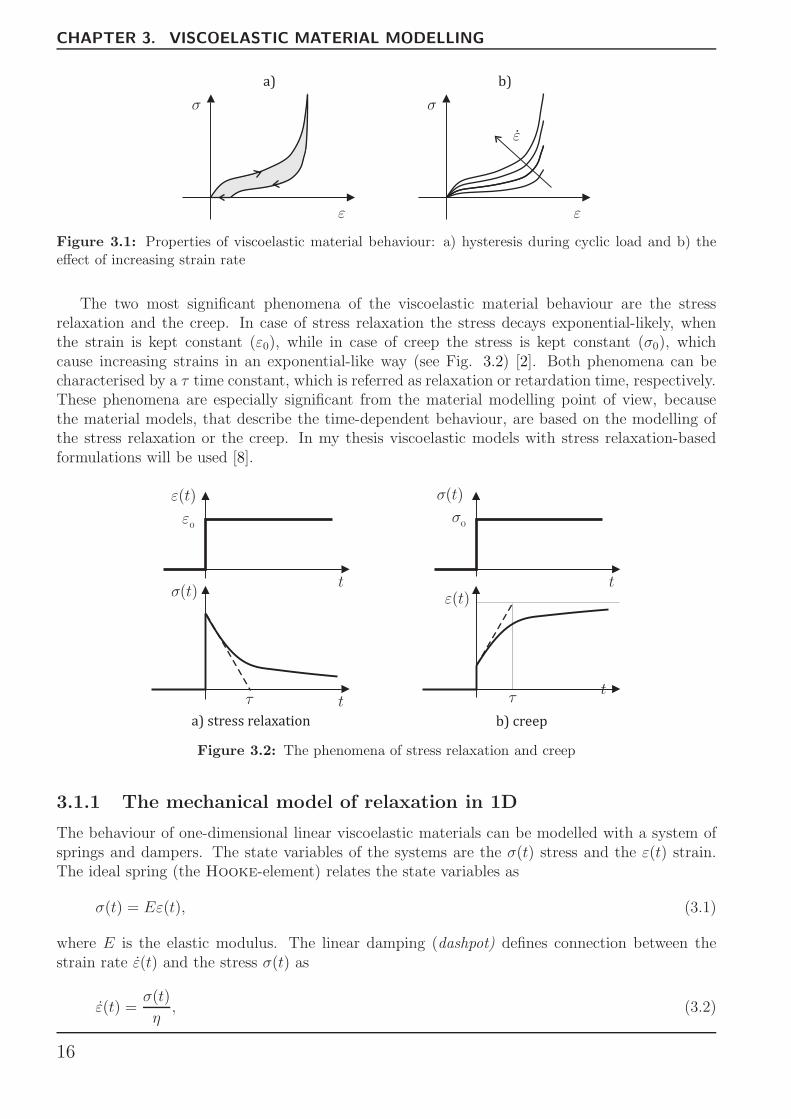
The two most significant phenomena of the viscoelastic material behaviour are the stressrelaxation and the creep. In case of stress relaxation the stress decays exponential-likely, whenthe strain is kept constant (ε0), while in case of creep the stress is kept constant (σ0), whichcause increasing strains in an exponential-like way (see Fig. 3.2) [2]. Both phenomena can becharacterised by a τ time constant, which is referred as relaxation or retardation time, respectively.These phenomena are especially significant from the material modelling point of view, becausethe material models, that describe the time-dependent behaviour, are based on the modelling ofthe stress relaxation or the creep. In my thesis viscoelastic models with stress relaxation-basedformulations will be used [8].

a) stress relaxation

"0

" t( )

t¾ t( )

t¿

¾0

" t( )t

¾ t( )

t¿

b) creep

Figure 3.2: The phenomena of stress relaxation and creep

3.1.1 The mechanical model of relaxation in 1D

The behaviour of one-dimensional linear viscoelastic materials can be modelled with a system ofsprings and dampers. The state variables of the systems are the σ(t) stress and the ε(t) strain.The ideal spring (the Hooke-element) relates the state variables as

σ(t) = Eε(t), (3.1)

where E is the elastic modulus. The linear damping (dashpot) defines connection between thestrain rate ε(t) and the stress σ(t) as

ε(t) =σ(t)

η, (3.2)

16

3.1. VISCOELASTIC MATERIAL BEHAVIOUR

( )a Maxwell ( )b Kelvin-Voigt ( )c Generalized-Maxwell

E

E

E∞

E1

E2

E3

EP

´1

´2

´3

´P

´

´

Figure 3.3: Mechanical models of time-dependent material behaviour

where η is the viscosity [19]. The serial configuration of the spring and the linear damping givesthe so-called Maxwell-element (see Fig. 3.3/a) [19], where the governing differential equationof the state variables becomes

ε(t) =σ(t)

η+

σ(t)

E. (3.3)

On the other hand, the parallel configuration of the spring and the dashpot is called Kelvin-Voigt-element (see Fig. 3.3/b) [19], while the corresponding differential equation can be obtainedas

σ(t) = Eε(t) + ηε(t). (3.4)

The viscoelastic material behaviour can be characterised with the differential equations in (3.3)and (3.4), which are the constitutive equations of linear viscoelasticity. For more complex cases,the so-called Generalized-Maxwell model is applied, in which several (P ) Maxwell-elements andone Hooke-element are assembled in parallel (see Fig. 3.3/c). In this approach the Hooke-element models the long-term elastic behaviour (i.e. when the load in infinitely slow), where E∞

is the long-term elastic modulus [2].

3.1.2 The stress solution for 1D loading

In the Generalized-Maxwell model the number of parallel Maxwell-elements is P , while ηk andEk denotes the parameters in the Maxwell-elements, respecitively. Using these parameterswe can introduce a time parameter for each element, namely τk = ηk/Ek. This leads, that theresultant time-dependent elastic modulus E(t) can be expressed as

E(t) = E∞ +

P∑

k=1

Ek exp

[

−t

τk

]

, (3.5)

which is written using the so-called Prony-series representation [19]. The stress solution can beobtained as the solution of the viscoelastic model, for a prescribed ε(t) strain history. The modeldefines the stress solution in 1D as a convolution (or hereditary) integral of the strain rate ε(t)and the time-dependent elastic modulus in (3.5), thus

σ(t) =

∫ t

0

E(t− s)ε(s)ds. (3.6)

The formula can be rewritten in an alternative, but equivalent form, which is based on theinstantaneous elastic response instead. In this form the instantaneous elastic and the viscoelastic

17

CHAPTER 3. VISCOELASTIC MATERIAL MODELLING

contributions can be separated, therefore using the formalism in Abaqus [5] the convolutionintegral is defined as

σ(t) = σ0(t)−P∑

k=1

ekτk

∫ t

0

σ0(t− s) exp

[

−s

τk

]

ds, (3.7)

where the instantaneous stress response σ0(t) can be obtained from the strain input and theinstantaneous elastic modulus E0 as,

σ0(t) = E0ε(t). (3.8)

The above introduced model also contains the so-called relative elastic moduli ek, which aredefined as

ek =Ek

E0. (3.9)

3.2 Finite strain viscoelasticity

The mechanical characteristic of the investigated open-cell polymer foams require obtaining vis-coelastic material models using finite strain theory. As a consequence the linear viscoelasticconstitutive equation in (3.7) cannot be applied for polymer-foams. Instead, the so-called visco-hyperelastic modelling approach has to be followed. These material models combines the hypere-lastic material model for nonlinear materials with finite strains and the time-dependent viscoelasticmaterial model [5].

The visco-hyperelastic material model can be obtained by reformulating the linear viscoelasticmaterial model using finite strain theory. A possible formulation of such visco-hyperelastic mate-rials are provided by Abaqus [5]. It should be noted, that in Abaqus version 6.9, the materialmodel was updated and reformulated, but for the Hyperfoam (Ogden–Hill’s) hyperelastic materialmodel the implementation is remained the previous (as in Abaqus version 6.8) [9]. Therefore,in my calculations the original formulation is applied. According to the Abaqus formalism, theconstitutive equation is defined for the Kirchhoff stress tensor (τ ) [5], where for compressible mate-rials the instantaneous Kirchhoff stress tensor (τ 0) can be splitted into hydrostatic and deviatoricparts as

τ 0(t) = τD0 (F(t)) + τH

0 (J(t)), (3.10)

where the hydrostatic part is the function of the J volume ratio, while the deviatoric part is relatedto the so-called distortional deformation gradient (F). The distortional deformation gradient canbe directly obtained from the deformation gradient F, as

F =FJ−1/3. (3.11)

In Abaqus version 6.7 [5] the visco-hyperelastic constitutive equation corresponding to finitestrain materials can be obtained by the following convolution integrals:

τD(t) = τD0 (t) + SYMM

∫ t

0

G(s)

G0F−1

t (t− s)τD0 (t− s)Ft(t− s)ds, (3.12)

τH(t) = τH0 (t) +

∫ t

0

K(s)

K0τH0 (t− s)ds. (3.13)

18

3.2. FINITE STRAIN VISCOELASTICITY

E1

E2

E3

t=0t

t s-

F(t)

F(t s- ) Ft(t s- )

reference

configuration

current

configuration

Figure 3.4: The representation of the Ft(t− s) relative deformation gradient

The hereditary integral of the deviatoric part is performed via the pull-back Ft(t−s) and push-forward F−1

t (t−s) operators. In order to ensure objectivity, the system is transformed firstly backinto the state corresponding to time t − s, where the convolution integral can be performed andthen transformed back into the spatial configuration. Finally, the symmetric part of the solutionis obtained by using the SYMM operator. The pull-back operator, illustrated in Fig. 3.4, ispractically a relative deformation gradient defined between the time instants t−s and t, therefore

Ft(t− s) = F(t− s)F−1(t). (3.14)

In the deviatoric part of the governing constitutive equation (3.12) G(t) and G0 are the time-dependent and the instantaneous shear moduli, respectively. Similarly, in the hydrostatic part(3.13) K(t) and K0 defines the time-dependent and the instantaneous bulk moduli, respectively.Similarly to equation (3.5) the time-dependent mechanical moduli can be written using the Prony-series representation as

G(t) = G0

(

g∞ +PG∑

k=1

gk exp

[

−t

τGk

]

)

, K(t) = K0

(

k∞ +PK∑

k=1

kk exp

[

−t

τKk

]

)

, (3.15)

where gk and kk are the relative, while g∞ and k∞ are the long-term moduli, respectively. For theso-called relaxation moduli the following condition holds:

g∞ +

PG∑

k=1

gk = k∞ +

PK∑

k=1

kk = 1. (3.16)

The substitution of (3.15) into the convolution integrals in (3.12) and (3.13) defines the con-stitutive equation of the material model as

τD(t) = τD0 (t)− SYMM

[

PG∑

k=1

gkτGk

∫ t

0

F−1t (t− s)τD

0 (t− s)Ft(t− s) exp

[

−s

τGk

]

ds

]

, (3.17)

τH(t) = τH0 (t)−

PK∑

k=1

kkτKk

∫ t

0

τH0 (t− s) exp

[

−s

τKk

]

ds. (3.18)

Based on the literature suggestions [5], we assume that the number of parameters in thedeviatoric and the hydrostatic parts are equal, thus PG = PK = P . Based on the assumption thatthe shear and the bulk moduli relax equally, it can be considered that the corresponding relativeshear and bulk moduli are the same, therefore gk = kk, furthermore the relaxation parameters are

19

CHAPTER 3. VISCOELASTIC MATERIAL MODELLING

also obtained to be equal, thus τGk = τKk = τk. After substituting the above introduced conditionsinto the constitutive equations in (3.17) and (3.18), the final form of the visco-hyperelastic materialmodel for open-cell polymer foams became

τD(t) = τD0 (t)− SYMM

[

P∑

k=1

gkτk

∫ t

0

F−1t (t− s)τD

0 (t− s)Ft(t− s) exp

[

−s

τk

]

ds

]

, (3.19)

τH(t) = τH0 (t)−

P∑

k=1

gkτk

∫ t

0

τD0 (t− s) exp

[

−s

τk

]

ds, (3.20)

where the instantaneous stress responses, τD0 (t) and τH

0 (t) are adopted from the Ogden–Hill’sHyperfoam material model, which was defined in (2.36).

3.3 Numerical implementation

The stress solution for visco-hyperelastic materials can be obtained as the solution of the de-rived constitutive equation in (3.19) and (3.20), where the prescribed λ(t) stretch-history in theinstantaneous stress response characterize the loading path. During the finite element analysis,it is required to solve the integrals efficiently. Therefore, a numerical integration scheme is alsoprovided by Abaqus [5], where solution is integrated forward in time.

Firstly, let us introduce τDk (t) and τH

k (t) internal deviatoric and hydrostatic stresses, respec-tively, which are defined as

τDk (t) = SYMM

[

gkτk

∫ t

0

F−1t (t− s)τD

0 (t− s)Ft(t− s) exp

[

−s

τk

]

ds

]

, (3.21)

τHk (t) =

gkτk

∫ t

0

τH0 (t− s) exp

[

−s

τk

]

ds. (3.22)

For the deviatoric stresses, the pull-back, the push-forward and the SYMM operators shouldalso be considered, thus a modified deviatoric stresses should be obtained as

τD0 (t) = SYMM

[

∆FτD0 (t)∆F−1

]

, (3.23)

τDk (t) = SYMM

[

∆FτDk (t)∆F−1

]

, (3.24)

where ∆F = Ft(t + ∆t). According to the integration scheme applied in Abaqus [5], the stresssolution at time t+∆t can be calculated as

τ (t+∆t) =

(

1−P∑

k=1

aigk

)

τD0 (t+∆t) +

P∑

k=1

bigkτD0 (t) +

P∑

k=1

ciτDk (t) +

(

1−P∑

k=1

aigk

)

τH0 (t+∆t) +

P∑

k=1

bigkτH0 (t) +

P∑

k=1

ciτHk (t), (3.25)

with

ai = 1−τk∆t

(1− ci); bi =τk∆t

(1− ci)− ci; ci = exp

[

−∆t

τk

]

. (3.26)

Therefore the stress solution at time t+∆t can be derived from the intantaneous and internalstress values at time instant t and t + ∆t. The detailed derivation of the integration scheme isprovided in Appendix B.

20

4Closed-form stress solutions

As it was introduced in Chapter 3, the mechanical behaviour of polymer foams can be modelled us-

ing visco-hyperelatic material models, where the corresponding hyperelastic constitutive equation

is the Ogden–Hill’s Hyperfoam model. Nevertheless, the model is obtained using the hereditary

integral of the input stetch-history function, therefore to obtain analytically the stress solution,

the convolution integrals in (3.19) and (3.20) should be solved.

In the literature, the closed-form solution corresponding any particular loading case has not

been provided yet, since the solution of the integral is quite complex. The main goal of this thesis

is to provide the closed-form solutions for the most common homogeneous deformations: uniaxial,

equibiaxial and volumetric compressions [9],[10].

4.1 Homogeneous deformations

Firstly, let us summarize the basic homogeneous deformations, for which the closed form solutions

are to be provided. In these cases the deformation is characterised by the deformation gradient

F . Based on the deformation gradient the principal stretches can also be obtained (λk), which in

case of time-dependent material behavior are considered to be time functions, thus

λk = λk(t). (4.1)

Based on the principal stretches, the instantaneous (time-independent) Kirchhoff stress tensor

(τ 0(t)), which appears in the visco-hyperelatic constitutive equation, can be expressed based on

the Ogden–Hill’s hyperelastic material model in (2.38). During our calculation the assumtion

βi = 0 will be applied as it was introduced for open-cell polymer foams in (2.30). Therefore, the

principal Kirchhoff stresses obtained from (2.38) can be simplified as

τk =N∑

i=1

2µi

αi

(λαik − 1) . (4.2)

21

CHAPTER 4. CLOSED-FORM STRESS SOLUTIONS

4.1.1 Uniaxial compression

E1

E3

E2

e1

e3

e2

1

¸1

a) before deformation b) after deformation

1

1

¸T

¸T

Figure 4.1: The kinematics of uniaxial compression

In case of uniaxial compression, the body is compressed in only one direction. This direction iscalled as longitudinal direction, and the corresponding stretch is denoted as λ1. In the other twoprincipal directions, which are referred as transversal directions, no load is applied. For isotropicmaterials the transversal stretches are identical, thus λ2 = λ3 = λT . Additionally, the body candeform freely in these directions, which leads that the transversal stresses are zero. The kinematicsof the loading case is presented in Fig. 4.1. Therefore, the deformation gradient becomes

F =

λ1 0 00 λT 00 0 λT

=

λ1 0 00 1 00 0 1

, (4.3)

where λT ≡ 1, because the βi = 0 assumtion is applied. Based on the description of uniaxialcomrpession the Kirchhoff stress tensor can be written as

τ=

τ1 0 00 0 00 0 0

. (4.4)

By substituting, the principal stretches back into the Ogden–Hill’s constitutive equation in(4.2), the instantaneous principal Kirchhoff stress solution can be expressed as

τ 0 (t) =

τ0 (t) 0 00 0 00 0 0

=

N∑

i=1

2µi

αi(λαi (t)− 1) 0 0

0 0 00 0 0

. (4.5)

It should be noted, that for βi = 0 case the uniaxial compression is identical with the so-called confined uniaxial deformation case, in which the stretches kept constant in the transversaldirection. In this case the body cannot deform freely in the transversal directions, thus stressappears. However, when the Poisson’s ratio is neglected, the load has no effect in the transversaldirections, this leads that the confined compression has the same kinematic description as theorginal uniaxial compression.

22

4.1. HOMOGENEOUS DEFORMATIONS

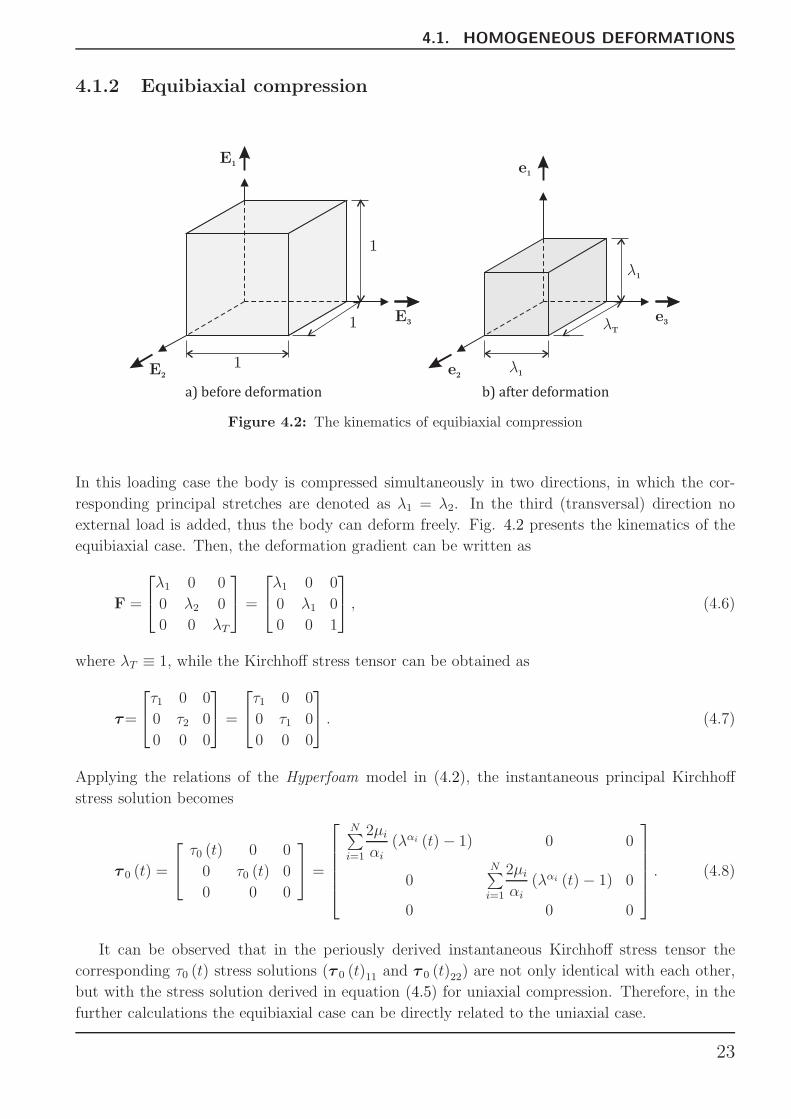
4.1.2 Equibiaxial compression

E1

E3

E2

e1

e3

e2

1

¸1

a) before deformation b) after deformation

1

1

¸1

¸T

Figure 4.2: The kinematics of equibiaxial compression

In this loading case the body is compressed simultaneously in two directions, in which the cor-

responding principal stretches are denoted as λ1 = λ2. In the third (transversal) direction no

external load is added, thus the body can deform freely. Fig. 4.2 presents the kinematics of the

equibiaxial case. Then, the deformation gradient can be written as

F =

λ1 0 0

0 λ2 0

0 0 λT

=

λ1 0 0

0 λ1 0

0 0 1

, (4.6)

where λT ≡ 1, while the Kirchhoff stress tensor can be obtained as

τ=

τ1 0 0

0 τ2 0

0 0 0

=

τ1 0 0

0 τ1 0

0 0 0

. (4.7)

Applying the relations of the Hyperfoam model in (4.2), the instantaneous principal Kirchhoff

stress solution becomes

τ 0 (t) =

τ0 (t) 0 0

0 τ0 (t) 0

0 0 0

=

N∑

i=1

2µi

αi

(λαi (t)− 1) 0 0

0N∑

i=1

2µi

αi(λαi (t)− 1) 0

0 0 0

. (4.8)

It can be observed that in the periously derived instantaneous Kirchhoff stress tensor the

corresponding τ0 (t) stress solutions (τ 0 (t)11 and τ 0 (t)22) are not only identical with each other,

but with the stress solution derived in equation (4.5) for uniaxial compression. Therefore, in the

further calculations the equibiaxial case can be directly related to the uniaxial case.

23

CHAPTER 4. CLOSED-FORM STRESS SOLUTIONS

4.1.3 Volumetric compression

E1

E3

E2

e1

e3

e2

1

¸1

a) before deformation b) after deformation

1

1

¸1

¸1

Figure 4.3: The kinematics of volumetric compression

In this loading case the body is compressed from each directions in the same way, therefore theprincipal stretches can be related as λ1 = λ2 = λ3 (see Fig. 4.3). Thus, the deformation gradientbecomes

F =

λ1 0 00 λ2 00 0 λ3

=

λ1 0 00 λ1 00 0 λ1

. (4.9)

Due to the isotropy, the stresses will be identical as well, thus the Kirchhoff stress tensor canbe expressed as

τ=

τ1 0 00 τ2 00 0 τ3

=

τ1 0 00 τ1 00 0 τ1

. (4.10)

Substituting back the relations of the hyperelastic material model in (4.2), the instantaneousprincipal Kirchhoff stress solution becomes

τ 0 (t) =

τ0 (t) 0 00 τ0 (t) 00 0 τ0 (t)

=

N∑

i=1

2µi

αi(λαi (t)− 1) 0 0

0N∑

i=1

2µi

αi

(λαi (t)− 1) 0

0 0N∑

i=1

2µi

αi(λαi (t)− 1)

. (4.11)

The result also suggests the same as in case of equibiaxial compression. The elements in the

diagonal are identical with each other and furthermore with the stress solution in equation (4.5).

Consequently, the stress solution of the volumetric case can also be related to the solution of

uniaxial compression.

24

4.1. HOMOGENEOUS DEFORMATIONS

4.1.4 Simple shear

E2

E1

E3

1

a) before deformation

1

1

e2

e1

e3

1

b) after deformation

1

°

1

Figure 4.4: The kinematics of volumetric compression

In case of simple shear, the upper side of the body is translated with γ, while the deformations

in all other directions are confined. The kinematics of the deformation is presented in Fig. 4.4.

Therefore, in the original coordinate system, the deformation gradient become

F0=

1 γ 0

0 1 0

0 0 1

, (4.12)

which also means that the volume ratio J = 1, i.e. the volume does not change. In the coordinate

system of the principal stretches the deformation gradient F can be expressed as

F =

λ1 0 0

0 λ2 0

0 0 λT

=

λ1 0 0

0 λ2 0

0 0 1

, (4.13)

which means, the Kirchhoff stress tensor τ can be written as

τ=

τ1 0 0

0 τ2 0

0 0 0

. (4.14)

In order to obtain τ1 and τ2 stresses, the principal direction should be determined. Using

eigenvalue and eigenvector calculations the principal stretches become

λ1 =1

2

(

γ +√

γ2 + 4)

, (4.15)

λ2 =1

2

(

−γ +√

γ2 + 4)

, (4.16)

λ3 = 1. (4.17)

25

CHAPTER 4. CLOSED-FORM STRESS SOLUTIONS

In this case the γ(t) function characterise the time-history of the deformation. Substitution

of equations in (4.15)-(4.17) into the hyperelastic constitutive equation in (4.2) gives for the

instantaneous Kirchhoff stress tensor

τ 0 (t) =

τ1(t) 0 0

0 τ2(t) 0

0 0 0

=

N∑

i=1

2µi

αi(λαi

1 (t)− 1) 0 0

0N∑

i=1

2µi

αi

(λαi2 (t)− 1) 0

0 0 0

, (4.18)

where λ1(t) =12

(

γ(t) +√

γ2(t) + 4)

and λ2(t) =12

(

−γ(t) +√

γ2(t) + 4)

. Unfortunately, these

result could not be related to solution of the uniaxial compression case in (4.5), furthermore it

can be clearly seen that the corresponding instantaneous stress responses are significantly more

complex than previous ones. Consequently, the stress response could not be solved analytically

for the simple shear case.

4.2 Solution of the hereditary integral

Based on the previously derived expressions, the closed-form stress response of the visco-hyperelasticmaterial can be obtained as the analytical solution of the hereditary integrals in (3.19) and (3.20).The analytical solvability of the convolution integrals strongly depend on the loading case, sincethe solution can be derived in closed-form only for the simplest deformations and strain histories.In the literature some attempts can be found, where the closed-form solution is derived for muchsimpler visco-hyperelastic model for rubber-like materials [8], but no analytical solution has beenprovided yet for the visco-hyperelastic material model using the Hyperfoam hyperelastic model. However, in case of open-cell polymer foams (where βi = 0) closed-form stress solution can bedeveloped for uniaxial compression [9],[10]. Based on the results the stress solutions of equibiaxialand volumetric compressions can also de defined.

In case of uniaxial compression the prescribed stretch history input is defined as

λ(t) =

{

1 + εt t ≤ T

1 + εT t > T, (4.19)

which means that the body is compressed with constant ε strain rate in a finite T time, then thestrain is kept constant. This stretch function can be substituted back into the solution of thehyperelastic model in (4.5). Since in the visco-hyperelastic constitutive equation the deviatoricand hydrostatic part of the solutions are separated, the instantaneous stress response should alsobe splitted, therefore

τD0 (t) = τ0 (t)

23

0 00 −1

30

0 0 −13

=

N∑

i=1

2µi

αi(λαi (t)− 1)

23

0 00 −1

30

0 0 −13

, (4.20)

τH0 (t) =

1

3τ0 (t) · I =

N∑

i=1

2µi

3αi

(λαi (t)− 1) · I, (4.21)

26

4.2. SOLUTION OF THE HEREDITARY INTEGRAL

where I is the second-order identity tensor. In the convolution integral the pull-back operatorF t (t− s) is also presented, which can be obtained using the relations in equations (4.19) and(3.14), thus

F =

λ (t) 0 00 1 00 0 1

, F t (t− s) =

λ(t−s)λ(t)

0 0

0 1 00 0 1

. (4.22)

Since, both τD0 (t) and F t (t− s) tensors are diagonal, the order of the tensor product can

be commuted, which leads that F t (t− s)F−1t (t− s) = I can be simplified. Additionally, for

diagonal tensors the SYM operator can also be simplified. Consequently, the convolution integralin (4.20) and 4.21) can also be simplified as

τD (t) =N∑

i=1

2µi

αi

(λαi (t)− 1)

23

0 00 −1

30

0 0 −13

−P∑

k=1

gkτk

t∫

0

N∑

i=1

2µi

αi

(λαi (t− s)− 1)

23

0 00 −1

30

0 0 −13

exp

[

−s

τk

]

ds, (4.23)

τH (t) =

N∑

i=1

2µi

3αi(λαi (t)− 1) · I −

P∑

k=1

gkτk

t∫

0

N∑

i=1

2µi

3αi(λαi (t)− 1) · Iexp

[

−s

τk

]

ds. (4.24)

These integrals could not be performed in one step, because λ (t) and τ 0 (t) also consist of twoparts: the uploading and the relaxation. Therefore, the hereditary integral is performed also intwo steps and the closed-form stress response is provided by separated functions for the uploadingand the relaxation, respectively. The input functions and the steps of the convolution integral aresummarized in Fig. 4.5.

tT

a)

¸0

tT

b)¸ t( )

¿0

- ( )¿ t

sT

c)

- ( - )¿ t s

t

e-s

st

d)

- ( - )¿ t s

t T-

e-s

I. II.

Figure 4.5: The prescribed a) stretch history input function λ (t), b) the intantaneous stress responseτ0 (t) and c)-d) the steps of the convolution integral for the uploading and the relaxation parts

27

CHAPTER 4. CLOSED-FORM STRESS SOLUTIONS

4.2.1 Uploading part

In the uploading part, when t ≤ T , after replacing λ (t) = 1+ εt stretch input function into (4.23)and (4.24) and performing the integral, the stress response can be provided as

τ (t) = τD (t) + τH (t) =

23

0 00 −1

30

0 0 −13

τ (t) +

13

0 00 1

30

0 0 13

τ (t) =

=

1 0 00 0 00 0 0

τ (t) , (4.25)

which means that the solutions satisfied the kinematic constrains for uniaxial compression. In thesolution the τ (t) longitudinal principal stress becomes

τ (t) = τ0 (t)−P∑

k=1

gk

(

N∑

i=1

2µi

αiηik

)

, (4.26)

where, ηik can be directly calculated from the material and load parameters as

ηik = e−

tτk − 1− e

−t+1/ετk

(

−1

ετk

)

−αi(

Γ

[

1 + αi,−1

τk ε

]

− Γ

[

1 + αi,−1 + tε

τkε

])

, (4.27)

in which Γ [a, z] is the so-called incomplete upper gamma function. By definition [20] [21], Γ [a, z]is provided as

Γ [ν, x] =

∞∫

x

tν−1e−tdt (4.28)

Further detalis about the incomplete gamma function are summarized in Appendix C.

4.2.2 Relaxation part

During the relaxation part, when t > T , the stretch input λ (t) = λ (T ) is constant. This leads,that the instantaneous stress response τ 0 (t) = τ 0 (T ) is also constant. The convolution intagralcan be performed as the sum of two integrals, namely

τD (t) = τD0 (T )−

P∑

k=1

gkτk

τD0 (T )

t−T∫

0

exp

[

−s

τk

]

ds+

t∫

t−T

τD0 (t− s) exp

[

−s

τk

]

ds

, (4.29)

τH (t) = τH0 (T )−

P∑

k=1

gkτk

τH0 (T )

t−T∫

0

exp

[

−s

τk

]

ds+

t∫

t−T

τH0 (t− s) exp

[

−s

τk

]

ds

, (4.30)

where firstly the integral on the [0, t−T ] interval defines the stresses related to the actual constantstretch value, while the integral on [t − T, t] defines the remaining effect of the uploading part.The final form of the integral is the same as in (4.25), while solution of the longitudinal principalstress can be obtained as

τ (t) = τ0 (T )

(

1−P∑

k=1

gk

(

1− exp

[

−t− T

τk

])

)

−P∑

k=1

gk

(

N∑

i=1

2µi

αi

ϑik

)

, (4.31)

in which ϑik depends on the parameters as

ϑik = e−

tτk − e

−t−Tτk − e

−1+εtετk

(

−1

ετk

)

−αi(

Γ

[

1 + αi,−1

τkε

]

− Γ

[

1 + αi,−1− T ε

τkε

])

. (4.32)

28

4.2. SOLUTION OF THE HEREDITARY INTEGRAL

4.2.3 Summary

In the previous steps the stress solution for uniaxial compression was developed. Since, theequibiaxial and volumetric compressions are directly obtained form to the uniaxial compressionusing the relations in (4.8) and (4.11), the closed for solutions are also determined for equibiaxialand volumetric compressions as well. Therefore, the solution can be expressed as

τU (t) =

τ0 (t) 0 00 0 00 0 0

, τB (t) =

τ0 (t) 0 00 τ0 (t) 00 0 0

, τ V (t) =

τ0 (t) 0 00 τ0 (t) 00 0 τ0 (t)

(4.33)

with

τ (t) =

τ0 (t)−P∑

k=1

gk

(

N∑

i=1

2µi

αiηik

)

t ≤ T

τ0 (T )

(

1−P∑

k=1

gk

(

1− exp[

− t−Tτk

])

)

−P∑

k=1

gk

(

N∑

i=1

2µi

αiϑik

)

t > T

(4.34)

where τU , τB and τ V denotes the uniaxial, the equibiaxial and the volumetric compressions,respectively. This closed-form solutions can be utilized in the parameter-fitting process, where themore accurate fitting approach can be applied based on the uniaxial stress solution of open-cellpolymer foams.

29

5Measurements

The accurate the finite element analysis of polyer foams requires to obtain the material parameters

in the visco-hyperelastic material model (3.19 and 3.20), which can be determined via parameter-

fitting based on measurement data. In accordance with the main fields of application, where the

load is dominantly compression, uniaxial compression test were performed on the investigated

memory foam material.

The goal of the measurement is to investigate experimentally the viscoelastic material be-

haviour and to provide measurement data for the parameter fitting process. As a result, the

stress-strain characteristics corresponding to different load cases are obtained, which also present

the most significant viscoelastic phenomena, namely as the strain rate dependency, the hysteresis

and the stress relaxation.

5.1 Introduction

The measurements were performed in the laboratory of the Department of Applied Mechanics

with an INSTRON 3345 Single Colum Universal Testing System. The load was measured by an

INSTRON model 2519-107 5kN load cell. In order to increase the cross section of the specimens an

additional compression platen were mounted to the system. The measurement layout is presented

in Fig. 5.1.

During experimental investigation of the time-dependent material behavior, the following two

compression tests were performed:

1. Relaxation test

2. Cyclic test with incremental loading

In both test the u(t) displacement was controlled, while the load F was the output, the

sampling interval was 0.01 s. The measurement were performed under similar environmental

conditions namely 22◦C air temperature and 44% relative humidity.

31

CHAPTER 5. MEASUREMENTS

Crosshead

Load cell

Compression platen

Additional platen

Specimen

Figure 5.1: The layout of the measurement using INSTRON Testing System

5.1.1 Specimens

The investigated memory foam is a commercial polyurethane foam, distributed by Csomaeszk

Kft in Hungary. The ”Memoryszivacs” memory foam sheet is applied in mattrasses and medical

products. The memory foam is sold in the size of 200× 160× 1.

The specimens for the compession test were cutted from the raw material sheet. The specimens

were created accordingly to the international standard of ISO-3386-1 [22]. The standard requires

the specimens to be right parallelepiped with a minimum width/thickness ratio of 2:1. The optimal

thickness is 50 mm, although when the specimens are thinner, the longitudinal length (L0) can be

heightened by plying specimens together. Additionally, it is recommeded that the cross section

should the as large as possible, but it should not overlap the compression platen. Based on the

recommendations in the standard the size of the specimens became 8× 8 cm and 8 piece of them

were plied together. The dimensions of the specimens are listed in Table 5.1, while its geometry

is presented in Fig. 5.2.

Material PolyurethaneThickness (t) 10 mmWidth of the specimen (w) 80 mmCross section (A0) 6400 mm2

Table 5.1: The dimensions of the specimens

32

5.1. INTRODUCTION

e1

e3

e2

w

L0

w

Figure 5.2: The geometry of specimens

5.1.2 Evaluation of measurements

During the measurements in every sampling point the corresponding load (F ) and displacement

(∆L) values were recorded. The initial separation of the platens H0 = 110 mm is bigger, than the

height (L0) of the specimen. Therefore, at the beginning of the measured load is zero, since the

platens to not touch the specimens. The actual starting point can be obtained by utilizing the

so-called slack correction method, which is presented in Fig. 5.3.

L1

F F

uu

L0

H0

H0Specimen

inflection point

originalmodified

Figure 5.3: The measurement layout and the slack correction method

Due to the specimen plying, in the initial region of the measured F − ∆L characteristic an

inflection point can be detected. This error can be corrected with the tangent line from the

inflection point, which also determined the L1 displacement corresponding to the starting point.

Using this L1 displacement value, the exact height of the specimen can be calculated as

L0 = H0 − L1 (5.1)

From the measured F − ∆L data, the longitudnial stretch (λ1) and the stress (P1) data can

be obtained as

λ1 = 1 +u

L0

, P1 = σ1 =F

A0

, (5.2)

33

CHAPTER 5. MEASUREMENTS

where the Cauchy and the 1st Piola–Kirchhoff stresses are identical, since the transversal (or

cross-directional) strains can be neglected according to the assumption in (2.30), i.e. λT = 1.

It should be noted, that due to the small sampling time (0.01 s), the measurement results

(data points) can be illustrated with continous curves.

5.2 Relaxation test

The time-dependent material behaviour can be characterised by the stress relaxation phneomena

(see Section 3.1), which can be investigated in ideal case as the stress response for unit step strain

input. In real measurement it means infinite strain rate at t = 0, therefore it is well-known that

only ramp test can be performed. In this case, the specimen is compressed with constant strain

rate in a finite T time and then the strain is kept constant, while the stress relaxes. In order to

have significant relaxation, the uploading strain rate (ε) should be as high as possible. During the

performed test on the investigated memory foam the crosshead speed was the highest possible,

namely v = 1000 mm/min, for the maximal strain umax = 85 mm and for the relaxation time

600 s were prescribed. The displacement input of the relaxation test is presented in Fig. 5.4.

t

u t( )

T

Figure 5.4: The prescribed time-history of the displacement in case of the relaxation test

The time of uploading (T ), the maximal longitudinal stretch (λmax) and the strain rate (ε)

are determined from the exact dimensions of the specimen obtained from equation (5.1). The

parameters of the relaxation test are listed in Table 5.2.

Time of uploading (T ) 4.792 sMaximal longitudinal stretch (λmax) 0.240198Strain rate (ε) −0.1585565 1/sExact height of the specimen (L0) 104.082 mm

Table 5.2: The parameters of the relaxation test

5.2.1 Results

The result of the measurement and the stress relaxation phenomena can be presented by the

Cauchy stress-time (σ − t) and the Cauchy stress- stretch (σ − λ) characteristics, which are

presented in Figs. 5.5 and 5.7.

34

5.2. RELAXATION TEST

¾[ ]MPa

¸[ ]-

Figure 5.5: The stress-stretch characteristic (σ − λ) in case of the relaxation test

¾[ ]MPa

t[ ]s

Figure 5.6: The stress response on the t ∈ [0, 400] domain in case of relaxation test

¾[ ]MPa

t[ ]s

Figure 5.7: The stress response on the t ∈ [0, 40] domain in case of relaxation test

35

CHAPTER 5. MEASUREMENTS

The characteristics shows, that the investigated memory foam shows significant viscoelacaticproperties, therefore our approach, which states that this particular material should be modelledusing visco-hyperelastic material models, is verified.

5.3 Cyclic test

Beside the relaxation test, the viscoelastic behaviour of the memory foram can be inveastigated viacyclic test. During this test the specimen is compressed incrementally with low strain rate in a way,that after every strain increment the strain kept constant and the stress relaxed. Similarly, thedownloading process is perfromed in increments. Due to the viscoelastic properties, the uploadingand the downing process follows different pathes due to the energy dissipation in the material.During the relaxation, the stress values tends to the long-term (time-independent) stress response,thus the results of the cyclic test can be applied in the parameter-fitting of the time-independenthyperelastic material model.

In case of the cyclic test the dispalcement increment was set ∆u = 8,5 mm, the crossheadspeed was v = 100 mm/min, while the relaxation intervals were tREL = 30 s. The prescribeddisplacement-history input funtion is presented in Fig. 5.8. The exact values of the strain rate(ε) and the strain increment (∆ε) can be calculated from the height of the specimen obtained in(5.1). Table 5.3 presents the measurement parameters.

ParametersMaximal longitudinal stretch (λmax) 0.23183Strain rate (ε) −0.01546 1/sStrain increment in the first step (∆ε0) 0.0723Strain increment (∆ε) 0.0773Exact height of the specimen (L0) 107.835 mm

Table 5.3: The parameters of the cyclic test

t

u t( )

Figure 5.8: The prescribed time-history of the displacement in case of the cyclic test

36

5.3. CYCLIC TEST

5.3.1 Results

The results of the cyclic test can be summarized by the Cauchy stress-time (σ− t) and the Cauchystress-stretch (σ − λ) characteristics, which are provided in Figs. 5.10 and 5.9. The results show,that the relaxation is significant in this loading case as well, when the applied rate of deformationwas lower. Additionally, the time-dependent behavior can be also represented by the σ−λ curve,where a hysteresis can be found, which reflects to the energy dissipated in the material.

¾[ ]MPa

t[ ]s

Figure 5.9: The stress response in case of the cyclic test

¾[ ]MPa

¸[ ]-

Figure 5.10: The stress-stretch characteristic (σ − λ) in case of the cyclic test

37

CHAPTER 5. MEASUREMENTS

5.4 Summary of the measurement results

The results of the performed uniaxial compression tests demonstate the time-dependent viscoelas-tic properties of the memory foam material. The results can be summarized on a common σ − λstress-stretch diagram (see Fig. 5.11). These characteristics show that the stress values in case ofthe relaxation test are higher than the stress values obtained by cyclic test, since the strain ratewere also higher in case of the relaxation test. Additionally, it can be clearly seen, that in therelaxation regions of both tests the stress values tends to the long-term (time-independent) stressresponse values, which lay inbetween the up- and downloading parts of the cyclic test.

¾[ ]MPa

¸[ ]-

relaxation test

cyclic test

Figure 5.11: The measured stress-stretch characteristics (σ − λ) in case of two different uniaxial com-pression tests

As the measurement results show, the material bahaviour of the memory foam requires visco-hyperelastic material modelling approach. Additionally, the recorded characteristics provides thesufficient data for the further parameter fitting process.

38

6Parameter fitting

The parameter fitting is the last step in the material modelling process. In this step the material

parameters are determined, which are included in the constitutive equation describing the material

behaviour. Based on the fitted material parameters the mechanical response could be investigated

in case of complex load cases using finite element analysis. Although, it should be emphasized

that the results of the finite element analysis are very sensitive to the material parameters both

qualitatively and quantitatively. Therefore, the material parameters should be fitted as accurately

as possible. Otherwise the results of the finite element analysis could be inaccurate.

The parameter fitting method is based on the analytical solution corresponding to the measured

load case. In case of the visco-hyperelastic material model, this analytical solution is not available,

therefore an alternative, so-called separated method is applied in the literature. However, the

closed-form stress solutions for uniaxial compression is derived in Section 4, thus the entire material

model can be fitted in one-step. This latter method provides a better solution for the parameters,

thus the finite element analysis will be more accurate [9],[10].

6.1 The method of parameter fitting

During the parameter fitting process the analytical solution of the material model is fitted to

measurement data points. Nevertheless, several methods are provided in the literature for the pa-

rameter fitting process. The least square fitting technique is the most commonly applied method,

where the global extremum of the error function is searched in p, the space of the unknown

parameters. In this method the error function is defined as

e =

N∑

i=1

[

fA(xi,p)− fM(xi)]2, (6.1)

where N is the number of measurement data points, fA the analitical function to be fitted, xi

the values of the independent variable at the measurement points, while fM(xi) denotes the

measured values at the measurement points. This multidimensional global extreme-value problem

39

CHAPTER 6. PARAMETER FITTING

cannot be solved analytically, therefore numerical methods have to be applied [2]. During my

calculations the "NMinimize" algorithm was applied, which is a bulit-in algorithm in Wolfram

Mathematica[23]. The algorithm finds the global minimum of a multidimensional function

using deterministic and stochastical methods. The available stochastical methods, which are

referred as "SimulatedAnnealing", "NelderMead" and "RandomSearch", search for the global

minimum from random points in the parameter space. The only available deterministic method,

the "DifferentialEvolution", follows the local gradient of the function to be minimized. It

should be noted, that there is not any general method, which finds the minimum in the best and

most effective way. The results of the extreme-value problem always depends on the function to

be minimized, futhermore it is common that the different methods provide different results for the

same problem [23].

In case of the investigated memory foam material, the goal of the parameter fitting method is to

determine both the viscoelastic and the hyperelastic parameters as it is provided in (4.34) based on

the measurement data of the stress relaxation test. The number of material parameters included in

the visco-hyperelastic model are: 2N (α1, α2...αN ;µ1, µ2...µN) parameters for the time-independent

hyperelastic model and 2P (g1, g2...gP ; τ1, τ2...τP ) parameters for the time-dependent viscoelastic

model. It means that altogether 2(N + P ) parameters should be fitted to our measurement data

in order to describe the visco-hyperelastic material behavior.

6.2 Parameter fitting algorithms in case of visco-hyperelastic

materials

In case of visco-hyperelastic material model the parameter fitting is even more complicated since

the exact stress solution should be obtained as the solution of the convolution integrals in (3.19)

and (3.20). In the literarure closed-form solution for the Hyperfoam-based visco-hyperelastic model

has not been published yet for any load case. Therefore, an alternative parameter fitting method

is adopted, which is called as separated fitting [8].

Cyclic test result

Interpolated long-term response

tT

Ideal strain history

Real strain history

tT

error

Ideal response

Real response

a) b) c) ¾

¸

¾"

"0

error

Real long-term response

Figure 6.1: The applied a) stretch input and the b)-c) fitting errors induced during the separated fittingmethod

The concept of this algorithm is to find the parameters for a visco-hyperelastic material by

separating the parameter fitting of the long-term behaviour and the time-dependent stress relax-

ation. In this approach the hyperelastic model is fitted to the long-term stress response, while

the viscoelastic parameters are fitted to the stress relaxation behaviour. The long-term behavior

40

6.3. SEPARATED FITTING OF PARAMETERS

is determined from cyclic compression-relaxation loading (see Fig. 5.9), where the data points

corresponding to the long-term behavior appears between the uploading and downloading curves.

The data points could be determined using interpolation from the corresponding stress minima

and maxima, usually as the mean value. This induces errors in the parameter fitting process. Ad-

ditionally, it is assumed that the stress relaxation test is performed using step loading. However,

it is well-known that in real measurements ramp loading is used instead of step loading, which

induces significant error in the fitted viscoelastic parameters. The fitting errors included during

the separated method are summarized and presented in Fig. 6.1, [7], [6].

In order to fit accurately the material model, it is essential to obtain the stress solution for

the ramp loading. Then, the entire material model can be fitted to the experimental data without

separating the long-term behavior and the relaxation behavior. In the literature the closed-form

stress solution is provided only for simpler, usually incompressible visco-hyperelastic material

models. The solution for the Hyperfoam-based model is not available, therefore this fitting method

has not been applied, yet. However, in Chapter 4 the analytical stress solution was derived for

uniaxial compression, therefore this makes it possible to apply the closed-form fitting approach in

case of the open-cell polymer foams as well.

6.3 Separated fitting of parameters

In the process of the separated fitting, the material parameters of the long-term (rate-independent)

stress response and the time-dependent stress relaxation behaviour are fitted separately using

different measurement data. The material parameters of the long-term hyperelastic material

model denoted as (αi, µi), while the stress relaxation is characterized using the Prony-parameters

(gi, τi). It should be noted, that the long-term hyperelastic parameters (αi, µi), are not equal with

the hyperelastic parameters (αi, µi) in the visco-hyperelastic constitutive equation in (3.19) and

(3.20), which were related to the instantaneous stress response. However, the long-term and the

instantaneous stress responses can be related as

τ0(t) =1

g∞τ∞(t) (6.2)

where g∞ = 1−∑

gi can be obtained from the gi time-dependent Prony-parameters. In Abaqus

[5] the hyperelastic parameters can be defined both for the long-term and the instantaneous stress

responses, thus it does not induce any further error during the fitting process.

6.3.1 Hyperelastic parameters

In order to fit the long-term hyperelastic parameters, the data points corresponding to the long-

term stress response should be determined. This can be related to the results of the cyclic test

(see Fig. 5.9). The relaxation parts of the cyclic test tend to the long-term stress response values,

therefore in ”infinite” time the required measurement points could be reached. Nevertheless, the

relaxation was finite in time, thus the stress values did not reached the long-term stress values. To

obtain the corresponding data points, firstly the local extremums were detected (the stress values

at the end of each relaxation session) and then, using linear interpolation, the data points could be

determined. In case of the measured memory foam material altogether 10 point could be defined,

which corresponds to the long-term stress response and for which the hyperelastic material model

41

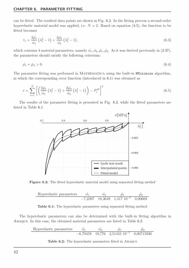
CHAPTER 6. PARAMETER FITTING

can be fitted. The resulted data points are shown in Fig. 6.2. In the fitting process a second-order

hyperelastic material model was applied, i.e. N = 2. Based on equation (4.5), the function to be

fitted becomes

τ1 =2µ1

α1

(

λ21 − 1

)

+2µ2

α2

(

λ21 − 1

)

, (6.3)

which contains 4 material parameters, namely α1, α2, µ1, µ2. As it was derived previously in (2.37),

the parameters should satisfy the following criterium:

µ1 + µ2 > 0. (6.4)

The parameter fitting was performed in Mathematica using the built-in NMinimize algorithm,

in which the corresponding error function (introduced in 6.1) was obtained as

e =

N∑

i=1

[(

2µ1

α1

(

λ21 − 1

)

+2µ2

α2

(

λ21 − 1

)

)

− PMi

]2

(6.5)

The results of the parameter fitting is presented in Fig. 6.2, while the fitted parameters are

listed in Table 6.1.

¸[ ]-

Cyclic test result

Fitted model

Interpolated points

¾[ ]MPa

Figure 6.2: The fitted hyperelastic material model using separated fitting methof

Hyperelastic parameters α1 α2 µ1 µ2

−7,2397 18,3649 1,417 10−7 0,00669

Table 6.1: The hyperelastic parameters using separated fitting method

The hyperelastic parameters can also be determined with the built-in fitting algorithm in

Abaqus. In this case, the obtained material parameters are listed in Table 6.2.

Hyperelastic parameters α1 α2 µ1 µ2

−6,70459 19,776 2,51455 10−7 0,00715936

Table 6.2: The hyperelastic parameters fitted in Abaqus

42

6.3. SEPARATED FITTING OF PARAMETERS

If we compare the results with the previously defined parameters in Table 6.1, it can be seen

that there is no significant difference. Therefore, during the further calculations those parameters

will be applied, which were fitted by the numerical algorithm in Mathematica.

The material parameters should also satisfy the Drucker-stability criteria defined in equations

(2.49)-(2.51). The stability was checked in Abaqus, where the results were exported into the

Job.dat file. The results of the stability analysis are listed in Table 6.3.

Load case StabilityUniaxial tension Stable for all strainsUniaxial compression Stable for all strainsBiaxial tension Stable for all strainsBiaxial compression Stable for all strainsVolumetric tension Stable for all volume ratiosVolumetric compression Stable for all volume ratiosSimple shear Stable for all shear strains

Table 6.3: The stability of the hyperelastic model in case of separated fitting method

As the results shows, the fitted hyperelastic model is stable for all deformations.

6.3.2 Prony parameters

The time-dependent viscoelastic behavior is characterized by the Prony-parameters (see equation

3.15), which can be fitted to the relaxation test results (see Fig. 5.6). The measurement results

are considered to be ideal relaxation response corresponding to step loading, in this case the stress

solution becomes

σ(t) = E0

(

e∞ +

P∑

k=1

ek exp

[

−t

τk

]

)

ε0 (6.6)

This yields, that the time-dependent relaxation modulus E(t) can be expressed as

E(t) =σ(t)

ε0= E0

(

e∞ +

P∑

k=1

ek exp

[

−t

τk

]

)

, (6.7)

which can be also obtained from the measurement data. The relation that e∞E0 = E∞ gives

E(t) =E∞

e∞

(

e∞ +P∑

k=1

ek exp

[

−t

τk

]

)

, (6.8)

where E∞ is calculated as the limit of the E(t), in our case E∞ = 0.00643 MPa. Dividing equation

(6.8) with the calculated E∞ value and expressing e∞ based on (3.16), the the function E(t) , which

should be fitted to the measurement data, becomes

E(t) =E(t)

E∞

=1

1−∑P

k=1 ek

(

1−P∑

k=1

ek +P∑

k=1

ek exp

[

−t

τk

]

)

, (6.9)

where the unknown material parameters are ek and τk. The so-called relaxation moduli can be

43

CHAPTER 6. PARAMETER FITTING

described with the same parameters, this yields that ek = gk = kk. Therefore, using the notation

of the visco-hyperelastic material model, the E(t) function is obtained as

E(t) =1

1−∑P

k=1 gk

(

1−P∑

k=1

gk +P∑

k=1

gk exp

[

−t

τk

]

)

. (6.10)

The same transformation should be performed on the measurement data as well. Firstly, the

stress relaxation function (σ−t) was divided with the corresponding strain ε0 = −0,7598, then the

long-term elastic modulus was obtained from E∞ = 0,00643 MPa. After dividing the measurement

data with E∞, the function in (6.10) can be fitted. For the order of the Prony series, P = 3 was

chosen and the fitting criteria τk > 0, gk > 0, g1 + g2 + g3 < 1 were defined. The fitting was

performed using the NMinimize built-in Mathematica algorithm. The result of the parameter

fitting is presented in Fig. 6.3, while the corresponding material parameters are listed in Table

6.4.

Prony parameters g1 g2 g3 τ1 τ2 τ30,61213 0,03739 0,01586 2,3221 20,6702 242,424

Table 6.4: The fitted Prony-parameters using separated fitting method

E[ ]-

t[ ]s

-

fitted model

measurement data

Figure 6.3: The time dependent modified elastic modulus E(t) and the fitted model using Prony-series

It should be noted, that for the viscoelastic parameters there is no available built-in fitting

algorithm in Abaqus, thus the parameter fitting can be performed using own fitting algorithm.

6.3.3 Validation with FEA

In the previous two subsections all material parameters have been identified in the visco-hyperelastic

constitutive equation using two separated algorithms for the hyperelastic and the viscoelastic pa-

rameters. The fitted mechanical model can be validated using finite element analysis (FEA). The

goal of the analysis is to investigate the accuracy of the fitted model based on real measurement

data. During the FEA, the relaxation test was analysed.

The geometry is an eighth model with unit cube, on which the same strain input was applied

as in case of the real measurement (see. Fig. 5.4). The mesh containes only one eight-node brick

44

6.3. SEPARATED FITTING OF PARAMETERS

element with reduced integration (C3D8R). On nodes 1-4 zero for all diplacements U1,2,3 = 0 was

prescribed, while on nodes 5-8 for the cross-directional displacements U2,3 = 0 was applied. Based

on the relaxation test data the longitudinal displacement was U1 = 0,7598 mm, while the time

of uploading was T = 4,792 s. The geometry of the FE model and the boundary conditions are

presented in Fig. 6.4.

E1

E3

E2

1

1

U1

11 2

4 3

5 6

7

8

1

U1

Figure 6.4: The finite element model and the applied constraints

The FEA was divided into two steps. In the first step the body is compressed with constant

strain rate, while in the second step the stain is kept constant, thus the stress could relax. The

steps were computed in defined increments in order to provide accurate numerical solution for

the nonlinear material model. The parameters of the steps applied during the FEA are listed in

Table. 6.5.

Step Start End Increment Number of IncrementsStep 1 0 s 4.792 s 0.01 s 480Step 2 4.792 s 100 s 0.2 s 500

Table 6.5: The parameters of the FEA

As the result of the analysis the principal longitudinal stress (σ1) and the strain (ε1) values

were queried from node 6 for all increments, which provides all necessary information for the

validation of the material model.

6.3.4 The results of the separated fitting

The results of the FEA, in which the fitted material model was applied, can be compared with the

measurement results of the relaxation test, which is presented in Fig. 6.5. As the result shows,

in the uploading part the fitted material model is close to the real measured data, while in case

of the stress relaxation part the error is significant. This can be explained by the approximation

that was applied during the fitting of stress relaxation, namely the relaxation data corresponds

to the ideal step load input. Addionally, the interpolation and the limited data points of the

long-term hyperelastic response also induces errors. It should be emphasized that in the literaute

there are several methods, which can reduce the errors in the Prony-parameters by modifying

45

CHAPTER 6. PARAMETER FITTING

the experimental data according to the method proposed by Zapas and Phillips [24], for instance.

But, these methods requires further calculations and data manipulations.

¾[ ]MPa

t[ ]s

fitted material model

measured relaxation

Figure 6.5: The comparison of the measured data with the fitted material model in case of separatedmethod

6.4 Closed-form parameter fitting

As the results of the separated fitting method shows, the material model will be inaccurate if the

parameters are fitted separately. Moreover, the inaccurate material model cause serious errors dur-

ing the FEA, which means that the calculated material behaviour differs significantly from the real

material response. In order to minimize the fitting errors, the material parameters should be fitted

in one-step using the closed-form stress solutions. This solution was derived for the investigated

memory foam material, when the loading is uniaxial compression. By adopting the stress solu-

tion in (4.34) all the 2N (α1, α2...αN ;µ1, µ2...µN) hyperelastic and the 2P (g1, g2...gP ; τ1, τ2...τP )

time-dependent Prony parameters can be identified simultaneously. This method increases the

computation time, but the fitted material parameter characterize the visco-hyperelastic material

behaviour more accurately [9],[10].

6.4.1 Identification of material parameters

Since the closed-form stress response τ (t) is obtained in equation (4.34), the material model can

be fitted directly to the stress relaxation data (see Fig. 5.6). The parameters of the loading case

were the strain rate ε = −0.1585565 1/s and the time of uploading T = 4,792 s. The parameter

fitting was performed again in Mathematica using the NMinimize global minimizer algorithm,

where the error function (to be minimized) was defined as

e =1

N1

N1∑

i=1

[

τ(

tM1

i

)

− σM1

i

]2+

1

N2

N2∑

i=1

[

τ(

tM2

i

)

− σM2

i

]2, (6.11)

where N1 and N2 denotes the measurement points in the uploading and the stress relaxation

parts, respectively. The applied material model contains a second-order hyperelastic (N = 2) and

a third-order Prony-series (P = 3).

46

6.4. CLOSED-FORM PARAMETER FITTING

Based on the conditions in (2.37), the criteria for the parameters were defined as

µ1 + µ2 > 0 τk > 0, gk > 0, g1 + g2 + g3 < 1 (6.12)

The identified visco-hyperelastic material parameters are presented in Table 6.6.

Hyperelastic parameters α1 α2 µ1 µ2

−2.1990 3.4435 0.000239 0.02235

Prony-parameters g1 g2 g3 τ1 τ2 τ30.84226 0.05311 0.03547 0.16031 0.84929 1.92388

Table 6.6: The material parameters in case of closed-form parameter fitting method

Since all parameters were identified, the stability of the hyperelastic model can also be checked

using the Drucker-stability criteria in Abaqus. The results of the stability analysis is presented

in Table 6.7.

Hyperelastic parameters StabilityUniaxial tension Stable for all strainsUniaxial compression Stable for all strainsBiaxial tension Stable for all strainsBiaxial compression Stable for all strainsVolumetric tension Stable for all volume ratiosVolumetric compression Stable for all volume ratiosSimple shear Stable for all shear strains

Table 6.7: The stability of the hyperelastic model using closed-form fitting method

Therefore, we can consider our modell stable. After that, similarly to the separated method,

the fitted model was validated with FEA in Abaqus. The FE model and all the settings were the

same as in case of the separated fitting (see Subsection 6.3.3). The results are presented in Fig. 6.6.

It should be remarked, that for the visco-hyperelastic material parameter there is not available

any built-in fitting subroutine in Abaqus. Consequently, the form closed-form parameter fitting

algorithm should be implemeneted by own codes for instance in Mathematica.

¾[ ]MPa

t[ ]s

fitted material model

measured relaxation

Figure 6.6: The results of the closed-form fitting

47

CHAPTER 6. PARAMETER FITTING

6.4.2 Predictions on the material behaviour

The identified material parameters enables us to investigate some material behaviour of the inves-

tigated memory foam material in case of further deformations and load cases. These investigation

are based on the analytical formulas, that were obtained in Chapter 5, namely uniaxial compres-

sion and simple shear.

¾[ ]MPa

¸[ ]-

instanta

neous

long-term

"= 2- [1/s]

"= 1- [1/s]

"=-0.5 [1/s]

"= 10 [1/s]-.

.

.

..

Figure 6.7: The stress solutions for the uniaxial uploading in case of different strain rates 1.

In case of uniaxial compression, the closed-form stress solution is obtained, thus the mechanical

responses can be provided, when the speed of deformation is different for instance. Therefore the

stetch input can be expressed as λ(t) = 1 + εt, where ε < 0. In the investigations, which can

also be considered as predictions, eight different strain rates are investigated including the time-

independent instantaneous and long-term cases. As a result the stress-stretch characteristics were

obtained, which are presented in Figs. 6.7 and 6.8.

instantaneous

long-term

"= 1- [1/s]

"=-0.5[1/s]

"= 10- [1/s]

.

.

.

¾[ ]MPa

¸[ ]-

"= 2- [1/s].

"= 4- [1/s].

Figure 6.8: The stress solutions for the uniaxial uploading in case of different strain rates 2.

48

6.4. CLOSED-FORM PARAMETER FITTING

The results present us the effect of the strain rate during the uploading process. Additionally,

it can also be seen, that the stress-stretch characteristics are always in between the long-term and

the intantaneous (time-independent) characteristics.

Secondly, the simple shear case was investigated, for which the stress solution could not be

solved analytically. In this case, only the instantaneous and long-term principal stress values can

be calculated as it was derived in (4.18). The characteristics are presented in Fig. 6.9.

°[ ]-¾[ ]MPa

instantaneous stress¾11

long-term stress¾11

instantaneous stress¾22

long-term stress¾22

Figure 6.9: The principal stress caharcteristics in case of simple shear

The simple shear characteristics also gives some details about the possible time-dependent

stress solutions, since the the curves should lay inbetween the long-term and the instanataneous

stress responses.

49

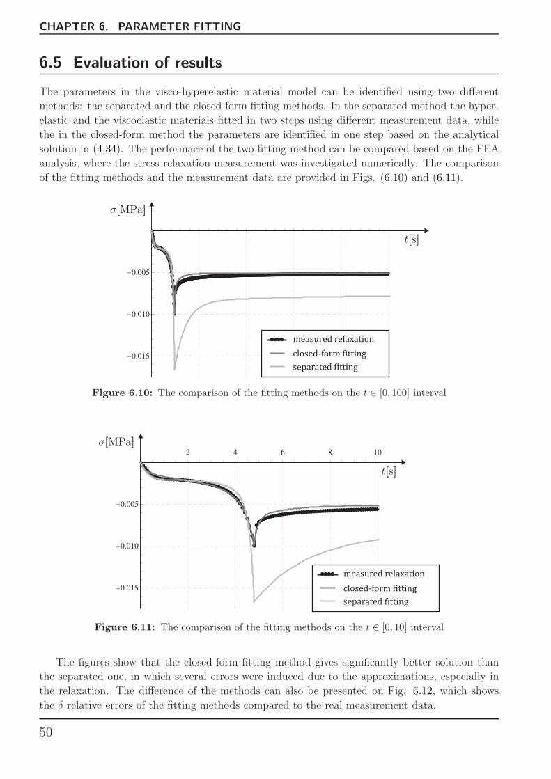
CHAPTER 6. PARAMETER FITTING

6.5 Evaluation of results

The parameters in the visco-hyperelastic material model can be identified using two different

methods: the separated and the closed form fitting methods. In the separated method the hyper-

elastic and the viscoelastic materials fitted in two steps using different measurement data, while

the in the closed-form method the parameters are identified in one step based on the analytical

solution in (4.34). The performace of the two fitting method can be compared based on the FEA

analysis, where the stress relaxation measurement was investigated numerically. The comparison

of the fitting methods and the measurement data are provided in Figs. (6.10) and (6.11).

¾[ ]MPa

t[ ]s

closed-form fitting

measured relaxation

separated fitting

Figure 6.10: The comparison of the fitting methods on the t ∈ [0, 100] interval

¾[ ]MPa

t[ ]s

closed-form fitting

measured relaxation

separated fitting

Figure 6.11: The comparison of the fitting methods on the t ∈ [0, 10] interval

The figures show that the closed-form fitting method gives significantly better solution than

the separated one, in which several errors were induced due to the approximations, especially in

the relaxation. The difference of the methods can also be presented on Fig. 6.12, which shows

the δ relative errors of the fitting methods compared to the real measurement data.

50

6.5. EVALUATION OF RESULTS

closed-form fitting

separated fitting

±[ ]%

t[ ]s

Figure 6.12: The relative errors of the fitting methods, compared to the measurement data

Consequently, it can be clearly seen that the closed-form fitting method improves the accuracy

of the time-dependent visco-hyperelastic material model, which also improves the performance of

the further numerical investigations using finite element method. Nevertheless, it should be noted,

that the accuracy of the closed-form fitting process can be further improved by adopting higher

order hyperelastic or Prony-series, which would also increase further the computation time during

the fitting process. However, as the results show in case of uniaxial compression the second-order

hyperelastic and third-order Prony-series give acceptable results and show properly the efficiency

and the accuracy of the closes-form fitting method compared to the separated one.

51

7Summary of results

7.1 Summary in English

Polymer foams are widely applied cellular materials in the field of industry and in everyday use

as well, due to their favourable mechanical behaviour. Therefore, there is a significant need to

understand and model their mechanical behaviour properly in order to improve the finite el-

ement analysis of such materials. Since the polymer foams shows time-dependent viscoelastic

properties, their mechanical behaviour can be modelled using special viscoelastic material mod-

els. Additionally, the deformation of polymer foams can be characterized by large strains and

deformations, thus the linear viscoelastic modelling approach cannot be applied and the so-called

visco-hyperelastic material models should be used instead. In this approach the viscoelastic mate-

rial model is combined with a hyperelastic model, which describes the time-independent behaviour

based on the corresponding strain energy function. The goal of my thesis was to investigate the

visco-hyperelastic material modelling in case of a particular commercial memory foam material,

which can be found in mattresses as well.

Firstly, I summarized the basis of hyperelasticity and introduced the Ogden–Hill’s compressible

hyperelastic material model and discussed its properties. This hyperelastic model is the only

widely applied compressible hyperelastic model, which can characterize the behaviour of polymer

foams. After that, the concept of viscoelasticity and the linear viscoelastic modelling approach

were summarized, in which the time-dependent material behaviour is characterised by Prony-

series. Finally, the visco-hyperelastic constitutive equation was obtained as the reformulation of

the linear viscoelastic model for finite strains based on the formalism applied in Abaqus.

Since the introduced visco-hyperelastic model defines the relation of the strain history and the

stress response in the form of a hereditary integral, the general stress response solution cannot

be obtained. Additionally, the analytical solution of this integral has not been provided for any

load case in the literature. Therefore, after summarizing the basic homogeneous deformations,

I have derived the closed-form stress solution in case of uniaxial compression. This analytical

solution can be directly related to the equibiaxial and volumetric compression deformations, thus

the solution for these deformations are also provided.

53

CHAPTER 7. SUMMARY OF RESULTS

The time-dependent mechanical behaviour of the memory foams was also investigated exper-

imentally by uniaxial compression tests, namely relaxation and cyclic tests. The results of the

measurements have shown that the behaviour of the memory foam material has viscoelastic prop-

erties, thus the visco-hyperelastic modelling approach is necessary. Besides, the compression tests

also provided data for the parameter identification process.

The material parameters was identified using parameter fitting methods based on the measure-

ment data. In my thesis two fitting approaches were applied: the separated and the closed-form

methods. In the separated case the the parameter-fitting of the long-term behavior and the stress

relaxation parameters are performed separately, while the closed-form solution identifies the pa-

rameters in one step. The closed-form parameter fitting method is based based on the previously

derived analytical stress solution. Therefore this is a novel method, which provides a more accu-

rate modelling approach for polymer foams. The performance of the fitted material models were

analysed in Abaqus and additionally the behaviour of the fitted model was also discussed for

some further loading cases as well. As a conclusion we can state that the derived closed-form

solution significantly improves the material modelling of polymer foams.

To summarize the contributions, in my thesis the modelling approaches of polymer foams have

been summarized and a proper visco-hyperelastic material model has been provided. Furthermore,

the closed-form stress solution for uniaxial compression was derived, which was utilized successfully

in the parameter fitting process.

54

7.2. SUMMARY IN HUNGARIAN - AZ EREDMENYEK OSSZEFOGLALASA

7.2 Summary in Hungarian - Az eredmenyek osszefoglalasa

A polimer habok szeles korben elterjedt sejtszerkezetu anyagok, amelyeket kedvezo mechanikai

tulajdonsagaik miatt nem csak az iparban, hanem a hetkoznapok soran is eloszeretettel alkalmaz-

nak. Emiatt jelentos az igeny arra, hogy pontos mechanikai modellt alkossunk viselkedesukrol. A

polimer habok mechanikai viselkedese idofuggo tulajdonsagokat is mutat, emiatt specialis viszkoe-

lasztikus anyagmodelleket kell alkalmaznunk a modellezes soran. Mivel azonban a polimer habok

deformacioi nagy alakvaltozasokkal es elmozdulasokkal jarnak, ezert a mechanikai viselkedesuket

a polimer habokra felırhato, idofuggo viszko-hiperelasztikus anyagmodellek segıtsegevel ırhatjuk

le. Azonban altalanos viszko-hiperelasztikus anyagmodell nem erheto el, az csak a megfeleloen

megvalasztott idofuggetlen viselkedest leıro hiperelasztikus es a relaxaciot leıro viszkoelasztikus

anyagmodellek otvozesevel allıthato elo. Dolgozatom celja, hogy vizsgaljam a viszko-hiperelaszti-

kus anyagmodellezes lehetoseget a kereskedelmi forgalomban is kaphato memoriahab alapanyag

eseten.

Dolgozatomban eloszor osszefoglaltam az idofuggetlen hiperelasztikus anyagmodellek alap-

jait, valamint ismertettem a polimer habok eseten alkalmazhato osszenyomhato Ogden–Hill-fele

Hyperfoam anyagmodellt, amelyet azAbaqus vegeselemes szoftverben hasznalt formalizmus alap-

jan ırtam fel. Ezt kovetoen kovetoen osszegeztem a viszkoelasztikus anyagi viselkedes megkozelıte-

set, a Prony-sorzatok alakjaban felırhato anyagmodellt, melyet eloszor kis- majd veges alakvalto-

zasok eseten definialtam. Az ıgy nyert viszko-hiperelasztikus konstitutıv egyenlet alkalmas az

idofuggo anyagi viselkedest mutato memoriahabok leırasara.

A viszko-hiperelasztikus anyagmodell eseteben a feszultseg es az alakvaltozas kozti kapcsolatot

egy konvolucios integral segıtsegevel lehet felırni, amely fugg a bemeno elmozdulas jeltol, emiatt

a feszultseg valasz nem allıthato elo altalanos alakban. Jelenleg a szakirodalomban sem erheto

el a vizsgalt anyagmodell zartalaku megoldasa, meg egyszeru terhelesek esetere se. Azonban

nyılt cellas habok egytengelyu terhelese eseten az anyagmodell megoldhato, a levezetes lepeseit

reszletesen bemutatom. Mivel az egytengelyu terheles eseten szamıtott analitikus megoldas kozvet-

lenul kapcsolodik a kettengelyu illetve a terfogati osszenyomashoz, az analitikus megoldast ebben

a ket terhelesi esetben is eloallıtottam.

A memoria habok viselkedesenek viszko-hiperelasztikus jelleget egytengelyu nyomomeresek

segıtsegevel is vizsgaltam. A meresek soran ket tesztet vegeztem el: nagy deformaciosebesseggel

torteno relaxacios merest, valamint egy ciklikus tesztet, amely soran a probatest fokozatosan lett

fel- es leterhelve. A meresi eredmenyek egyertelmuen igazoltak a memoria hab alapanyag idofuggo

mechanikai tulajdonsagait.

A meresek alapjan a felırt anyagmodellben szereplo anyagparameterek illesztesevel is foglalkoz-

tam, melynek soran ket parameterillesztesi megkozelıtest is alkalmaztam. A szetvalasztott modszer

lenyege, hogy a gorbeillesztest az idofuggetlen (hiperelasztikus) es az idofuggo (Prony-sorozatok)

anyagmodellekre kulon lehet elvegezni. A zart alaku modszer eseteben az analitikus feszultseg

valasz fuggveny alapjan egy lepesben illesztheto valamennyi anyagparameter. Ez egy uj parameter-

illesztesi eljaras polimer habok eseteben, mivel a zart alaku feszultseg valasz fuggveny nem erheto

el a szakirodalomban. Az illesztett anyagmodellek pontossagat vegeselemes analızis segıtsegevel

ellenoriztem. Az eredmenyek alapjan elmondhato, hogy a zart alaku illesztes segıtsegevel mertek-

ben javıthato az illesztett anyagmodell pontossaga, amely a kesobbi vegeselemes analıziseket pon-

tosabba es megbızhatobba teszi.

Osszegezve, a dolgozatomban ismertettem a memoria habok mechanikai modellezeset, felırtam

az anyagi viselkedest leıro mechanikai modellt, valamint eloallıtottam a zart-alaku megoldast,

amely lehetove teszi az anyagparameterek pontos illeszteset.

55

56

Appendix

57

ARelation of the Hyperfoam material model and

the Hooke’s law

The parameters in the Ogden–Hill’s compressible hyperelastic (Hyperfoam) material model cannotbe chosen freely, because certain physical conditions have to be satisfied during the parameterfitting process. One of these conditions states that the linearized form of the nonlinear materialmodel should be equal with the Hooke’s law in case of small strains. The linearization is performedaround the undeformed state, i.e. when λi = 1. Firstly, let us introduce a modified stretch-measure(λ∗

i ) [25] as

λ∗

i = λiJ−1/3. (A.1)

Based on this stretch-measure, the originally applied strain energy function W (λ1, λ2, λ3) canbe rewritten as

W (λ1, λ2, λ3) = W ∗(λ∗

1, λ∗

2, λ∗

3, J), (A.2)

where λ∗

3 can be expressed as the function of λ∗

1 and λ∗

2 using the relation λ∗

3 = (λ∗

1λ∗

2)−1. Substi-

tuting this into (A.2) the simplified strain energy function W ∗ becomes

W ∗(λ∗

1, λ∗

2, J) = W ∗(λ∗

1, λ∗

2, (λ∗

1λ∗

2)−1 , J). (A.3)

Based on this formulation, the initial moduli of the material model can be related to the partialderivatives of the strain energy function in (A.3), which are evaluated at the undeformed state,i.e λ∗

1 = 1, λ∗

2 = 1 and J = 1 [25]. Thus

K =∂2W ∗

∂J2(1, 1, 1), (A.4)

µ0 =∂2W ∗

∂λ∗21

(1, 1, 1) =∂2W ∗

∂λ∗22

(1, 1, 1) = 2∂2W ∗

∂λ∗

1∂λ∗

2

(1, 1, 1), (A.5)

where K is the initial bulk modulus and µ0 the initial shear modulus.

59

APPENDIX A. RELATION OF THE HYPERFOAM MATERIAL MODEL AND THEHOOKE’S LAW

In the Ogden–Hill’s hyperelastic constitutive equation according to theAbaqus [5] formulationthe corresponding strain energy function can be written as

W =

N∑

i=1

2µi

α2i

(

λαi1 + λαi

2 + λαi3 − 3 +

1

βi

(

J−αiβi − 1)

)

, (A.6)

which, after substituting the relations in (A.1) back, leads that the W ∗ function becomes

W ∗(λ∗

1, λ∗

2, J) =N∑

i=1

2µi

α2i

(

(

λ∗

1J1/3)αi

+(

λ∗

2J1/3)αi

+

(

J1/3

λ∗

1λ∗

2

)αi

− 3 +1

βi

(

J−αiβi − 1)

)

. (A.7)

After expressing and evaluating the partial derivatives in (A.4) and (A.5), the initial modulican be expressed as

µ0 =

N∑

i=1

µi (A.8)

K =N∑

i=1

2µi

(

1

3βi

)

. (A.9)

In the Hooke’s law the conditions for the shear and the bulk moduli are µ0 > 0 and K > 0,respectively. Using the derived expressions in (A.8) and (A.9) leads that

µ0 =

N∑

i=1

µi > 0, K =

N∑

i=1

2µi

(

1

3+ βi

)

> 0, (A.10)

from which the conditions of the material parameters in the Ogden–Hill’s Hyperfoam materialmodel becomes

N∑

i=1

µi > 0, βi > −1

3(A.11)

It should be noted that the condition βi > −1/3 is stricter than the necessary condition forthe βi parameters, which significantly limits the possible domain of parameters. Although, thiscondition is applied in the literature and in Abaqus as well [5].

60

BNumerical implementation of visco-hyperelastic

model

The following derivation steps follows the structure of the Theory Guide in Abaqus [5]. Based onthe definition of the visco-hyperelastic constitutive equation in Abaqus [5], the Kirchhoff-stresssolutions can be obtained as

τD(t) = τD0 (t)− SYMM

[

P∑

k=1

gkτk

∫ t

0

F−1t (t− s)τD

0 (t− s)Ft(t− s) exp

[

−s

τk

]

ds

]

, (B.1)

τH(t) = τH0 (t)−

P∑

k=1

gkτk

∫ t

0

τH0 (t− s) exp

[

−s

τk

]

ds, (B.2)

where τD(t) is the deviatoric and τH(t) the hydrostatic part of the Kirchhoff stress tensor (τ ).Let us introduce the so-called internal stresses, associated with each term of the series

τDk (t) = SYMM

[

gkτk

∫ t

0

F−1t (t− s)τD

0 (t− s)Ft(t− s) exp

[

−s

τk

]

ds

]

, (B.3)

τHk (t) =

gkτk

∫ t

0

τH0 (t− s) exp

[

−s

τk

]

ds. (B.4)

The above introduced stresses are stored in each material point and integrated forward in time.We assume, that the stess solution at time t is known and we need to define the solution at timet + ∆t. The numerical integration of the convolution integrals in (B.1) and (B.2) are performedseparately for the deviatoric and the hydrostatic parts.

B.1 Integration of the hydrostatic stress

The internal hydrostatic stress values at time t +∆t can be obtained from

τHk (t+∆t) =

gkτk

∫ t+∆t

0

τH0 (t +∆t− s) exp

[

−s

τk

]

ds. (B.5)

61

APPENDIX B. NUMERICAL IMPLEMENTATION OF VISCO-HYPERELASTIC MODEL

Introducing t = s−∆t it follows that

τHk (t+∆t) =

gkτk

exp

[

−∆t

τk

]∫ 0

−∆t

τH0 (t− t) exp

[

−t

τk

]

dt+ exp

[

−∆t

τk

]

τHk (t) (B.6)

To perform the integral we assume that τH0 (t − t) is a linear function over the increment,

therefore

τH0 (t− t) =

(

1 +t

τk

)

τH0 (t)−

t

τkτH0 (t+∆t) −∆t ≤ t ≤ 0. (B.7)

Substitution back into (B.6) yields

τHk (t+∆t) =

gkτk

exp

[

−∆t

τk

] ∫ 0

−∆t

[(

1 +t

τk

)

τH0 (t)−

t

τkτH0 (t+∆t)

]

exp

[

−t

τk

]

dt

+exp

[

−∆t

τk

]

τHk (t). (B.8)

After expressing the integrals, the solution at the end of the increment becomes

τHk (t+∆t) =

[

1−τk∆t

(

1− exp

[

−∆t

τk

])]

gkτH0 (t+∆t) +

[

τk∆t

(

1− exp

[

−∆t

τk

])

− exp

[

−∆t

τk

]]

gkτH0 (t) + exp

[

−∆t

τk

]

τHk (t), (B.9)

which can be written in a simplified form as

τHk (t+∆t) = aigkτ

H0 (t+∆t) + bigkτ

H0 (t) + ciτ

Hk (t), (B.10)

where

ai = 1−τk∆t

(1− ci); bi =τk∆t

(1− ci)− ci; ci = exp

[

−∆t

τk

]

(B.11)

B.2 Integration of the deviatoric stress

The internal deviatoric stress values at time t+∆t can be obtained from

τDk (t+∆t) = SYMM

[

gkτk

∫ t+∆t

0

F−1t+∆t(t+∆t− s)τD

0 (t+∆t− s)Ft+∆t(t +∆t− s) exp

[

−s

τk

]

ds

]

.

(B.12)

Where the push-back operator related between time t and t+∆t becomes

Ft+∆t(t− s) = Ft(t− s)Ft+∆t(s). (B.13)

Introducing t = s−∆t, ∆F = Ft(t +∆t) and a new variable τD for which

τD0 (t) = SYMM

[

∆FτD0 (t)∆F−1

]

, (B.14)

τD0 (t+∆t) = τD

0 (t+∆t), (B.15)

τDk (t) = SYMM

[

∆FτDk (t)∆F−1

]

, (B.16)

62

B.3. TOTAL STRESS SOLUTION

relation hold, the integral simplifies to

τDk (t+∆t) =

gkτk

exp

[

−∆t

τk

]∫ 0

−∆t

τD0 (t− t) exp

[

−t

τk

]

dt + exp

[

−∆t

τk

]

τDk (t). (B.17)

To perform the integral we assume that τD0 (t− t) is a linear function over the increment, therefore

τD0 (t− t) =

(

1 +t

τk

)

τD0 (t)−

t

τkτD0 (t+∆t) −∆t ≤ t ≤ 0. (B.18)

Substituting back into (B.17), and performing the integration, we get exactly the same formof the stress solution as in (B.10) and (B.11), thus

τDk (t+∆t) = aigkτ

D0 (t+∆t) + bigkτ

D0 (t) + ciτ

Dk (t), (B.19)

where

ai = 1−τk∆t

(1− ci); bi =τk∆t

(1− ci)− ci; ci = exp

[

−∆t

τk

]

. (B.20)

B.3 Total stress solution

From the previously derived hydrostatic and deviatoric internal stress solutions in (B.10) and(B.19), respectively, the total stress at time t++∆t can be expressed as

τ (t+∆t) = τ 0(t− s)−P∑

k=1

τDk (t+∆t)−

P∑

k=1

τHk (t +∆t) (B.21)

which with equations (B.10) and (B.19) can also be written as

τ (t+∆t) =

(

1−P∑

k=1

aigk

)

τD0 (t+∆t) +

P∑

k=1

bigkτD0 (t) +

P∑

k=1

ciτDk (t) +

(

1−P∑

k=1

aigk

)

τH0 (t+∆t) +

P∑

k=1

bigkτH0 (t) +

P∑

k=1

ciτHk (t), (B.22)

with

ai = 1−τk∆t

(1− ci); bi =τk∆t

(1− ci)− ci; ci = exp

[

−∆t

τk

]

. (B.23)

63

CThe incomplete gamma function

The following summary of the upper incomplete gamma function Γ(ν, x) , which occurred in ourcalculations, is based on Spanier and Oldham: An atlas of functions [20] and the documentationsprovided by Wolfram Mathword [26], [21].

C.1 The (complete) gamma function

The (complete) gamma function Γ(n) is defined to be an extension of the factorial to complex andreal number arguments, which is related to the factorial in case of natural numbers as

Γ(n) = (n− 1)!. (C.1)

Generally, the (complete) gamma function is defined as a definite integral for all Re(z) > 0. Apossible formulation of this function is called as Euler’s integral form, in which

Γ(z) =

∫

∞

0

tz−1e−tdt, (C.2)

which can be alternatively given as

Γ(z) =

∫ 1

0

[

ln

(

1

t

)]z−1

dt. (C.3)

The complete gamma function can be further generalized using the so-called incomplete gammafunctions, which by definition satisfy

Γ(ν) = Γ(ν, x) + γ(ν, x), (C.4)

where Γ(ν, x) is the so-called upper incomplete gamma function and γ(ν, x) the lower incompletegamma function. The functions contain two variables: ν is called as the parameter, while x is theargument in both incomplete gamma functions. The adjective ”incomplete” reflects the restrictedranges of the definite integral compared to the complete gamma function in (C.2). The adjectives”upper” and ”lower” specifies that the particular incomplete gamma function is defined on whichrange of the x > 0 domain.

65

APPENDIX C. THE INCOMPLETE GAMMA FUNCTION

C.2 The upper incomplete gamma function

The upper incomplete gamma function is defined via an improper integral as

Γ(ν, x) =

∫

∞

x

tν−1e−tdt, (C.5)

for all Re(ν) > 0 and x > 0. Using the above introduced notation, the (complete) gamma functionΓ(ν) can be related to the upper incomplete gamma function as

Γ(ν) = Γ(ν, 0). (C.6)

When the parameter (ν) is a natural number, then the function can also be expressed usingthe exponential sum as

Γ(n, x) = (n− 1)!e−xn−1∑

k=0

xk

k!. (C.7)

The definition of the function in (C.5) can be extended to Re(z) < 0 by utilizing the recursionformula. Therefore

Γ(ν, x) =xνe−x

Γ(1− ν)

∫

∞

0

t−νe−t

t+ xdt. (C.8)

C.3 Special cases

For some special values of ν and x, the upper incomplete gamma function reduces to other well-known functions, like

Γ

(

1

2, x

)

=√πerfc

(√x)

, (C.9)

where erfc(x) denotes the complementer Gauss error function, or

Γ (0, x) =

{

−Ei(−x)− iπ, ha x < 0−Ei(−x), ha x > 0

}

. (C.10)

where Ei(x) is the so-called exponential integral function. Furthermore

Γ (ν + 1, x) = νΓ (ν, x) + xνe−x. (C.11)

66

Bibliography

[1] M. Ashby, H. Shercliff, and D. Cebon. Materials: Engineering, Science, Processing andDesign. Butterworth-Heinemann, 2007.

[2] G. Silber and C. Then. Preventive Biomechanics. Springer, 2013.

[3] N. Mills. Polymer foam handbook: Engineering and Biomechanics Applications and DesignGuide. Butterworth-Heinemann, 2006.

[4] Wikipedia. Memory foamDownloaded: 2015. 10. 21.

[5] Dassault Systemes. Abaqus, version 6.14-2. 2015.URL: www.3ds.com/products-services/simulia/products/abaqus/.

[6] S. Lee and W.G. Knauss. A note on the determination of relaxation and creep data fromramp tests. Mechanics of Time-Dependent Materials, (4):1–7, 2000.

[7] W.G. Knauss, I. Emri, and H. Lu. Handbook of Experimental Solid Mechanics: Mechanics ofPolymers - Viscoelasticity. Springer, 2008.

[8] S.M. Goh, M.N. Charalambides, and J.G.Williams. Determination of the constitutive con-stants of non-linear viscoelastic materials. Mechanics of Time-Dependent Materials, (8):255–268, 2004.

[9] A. Kossa and Sz. Berezvai. Visco-hyperelastic characterization of polymeric foam materials.In 32nd International Danubia-Adria Symposium on Advances in Experimental Mechanics.Slovakia, 2015.

[10] A. Kossa and Sz. Berezvai. Visco-hyperelastic characterization of polymeric foam materials.MaterialsToday: Proceedings, (Submitted), 2015.

[11] I. Dorghi. Mechanics of Deformable Solids. Springer, 2000.

[12] A. F. Bower. Applied mechanics of solids. CRC Press, 2010.

[13] EA. de Souza Neto, D. Peric, and DRJ. Owen. Computational methods for plasticity: theoryand application. John Wiley & Sons Ltd., 2008.

[14] ANSYS Inc. Ansys mechanical, version 13.5, 2015URL: www.ansys.com.

[15] MSC Softwares. Marc, 2015URL: www.mscsoftware.com/product/marc.

67

BIBLIOGRAPHY

[16] R. W. Ogden. Large deformation isotropic elasticity: On the correlation of theory andexperiment for compressible rubberlike solids. Proceedings of the Royal Society of London,Series A, Mathematical and Physical Sciences, (328):567–583, 1972.

[17] R. Hill. Aspects of invariance in solid mechanics. Advances in Applied Mechanics, (18):1–78,1978.

[18] B. Storakers. On material representation and constitutive branching in finite compressibleelasticity. Journal of the Mechanics and Physics of Solids, (34):125–145, 1986.

[19] S. P. C. Marques and G. J. Creus. Computational Viscoelasticity. Springer, 2012.

[20] J. Spanier and K.B. Oldham. An atlas of functions. Springer, 1987.

[21] Wolfram. Mathword: Incomplete gamma functionURL: mathworld.wolfram.com/IncompleteGammaFunction.html.

[22] International Organization for Standardization (ISO) EN ISO 3386-1. Polymeric materials,cellular flexible - determination of stres-strain characteristic in compression - part 1: Low-density meaterials, 1986.

[23] Wolfram. Mathematica, version 9.0URL: www.wolfram.com/mathematica.

[24] L.J. Zapas and J.C. Phillips. Simple shearing flows in polyisobutylene solutions. Journal ofResearch of the National Bureau of Standards, 75(1), 33-41 1971.

[25] R. W. Ogden. Elastic deformations of rubberlike solids. Mechanics of Solids. The RodneyHill 60th Anniversary Volume, pages 499–537, 1982.

[26] Wolfram. Mathword: Gamma functionURL: mathworld.wolfram.com/GammaFunction.html.

68