Embed Size (px)
Citation preview

Int. J. , Vol. x, No. x, xxxx 1
Copyright © 200x Inderscience Enterprises Ltd.
Estimation of running resistance of electric trains based on on-board telematics system
Szilárd Aradi
Department of Control for Transportation and Vehicle Systems,
Budapest University of Technology and Economics,
H-1111 Műegyetem rkp. 3., Budapest, Hungary
E-mail: [email protected]
Tamás Bécsi*
Department of Control for Transportation and Vehicle Systems,
Budapest University of Technology and Economics,
H-1111 Műegyetem rkp. 3., Budapest, Hungary
E-mail: [email protected]
*Corresponding author
Péter Gáspár
Institute for Computer Science and Control,
Hungarian Academy of Sciences,
H-1111 Kende u. 13-17, Budapest, Hungary
E-mail: [email protected]
Abstract: Advances in railway telematics and the large amount of data obtained from train services
enable the development of methods that are capable of further improving energy efficiency through
the evaluation, control or prediction of energy utilization of the railways. The paper proposes a
method for determining the longitudinal running resistance of electric trains based on the
measurements of on-board telemetric units of the locomotives. The purpose of the algorithm is to
resolve the parameters of the commonly used polynomial resistance formula for specific locomotive-
rolling stock types. In contrast with the classic measurements, such as tractive effort, dynamometer
or drawbar and the coasting methods the algorithm uses data from actual train runs, hence there is
no need for closed test tracks or special measurement scenarios, although, naturally, the
measurement conditions, such as track inclinations and rolling stock loads must be known.
Keywords: rail transport; rail vehicles; running resistance; parameter estimation, telematics.
Biographical notes: Szilárd Aradi received the M.Sc. degrees from the Faculty of Transportation
Engineering and Vehicle Engineering, Budapest University of Technology and Economics in 2005.
Since 2005 he has been a PhD student and since 2009 he has been an assistant lecturer at the
Department of Control for Transportation and Vehicle Systems, Budapest University of Technology
and Economics. His research interests include embedded systems, communication networks, vehicle
mechatronics and predictive control. His research and industrial works have involved railway
information systems, vehicle on-board networks and vehicle control.
Tamás Bécsi received both the M.Sc. and Ph.D. degrees from the Faculty of Transportation
Engineering and Vehicle Engineering, Budapest University of Technology and Economics in 2002

Author
and 2008, respectively. Since 2002 he has been a PhD student, since 2005 he has been an assistant
lecturer and since 2014 he has been a senior lecturer at the Department of Control for Transportation
and Vehicle Systems, Budapest University of Technology and Economics. His research interests
include linear systems, embedded systems, traffic modeling and simulation. His research and
industrial works have involved railway information systems, vehicle control and image processing.
Péter Gáspár received both the M.Sc. and Ph.D. degrees from the Faculty of Transportation
Engineering and Vehicle Engineering, Budapest University of Technology and Economics in 1985
and 1997, respectively, and the D.Sc. degree in control from the Hungarian Academy of Sciences
(HAS) in 2007. Since 1990 he has been a senior research fellow at the Systems and Control
Laboratory (SCL), Computer and Automation Research Institute, HAS and since 2007 he has been a
research advisor. He is Head of the Vehicle Dynamics and Control Research Group within SCL. He
is the head of the Department of Control for Transportation and Vehicle Systems, Budapest
University of Technology and Economics. He is a member of IFAC Technical Committee on both the
Automotive Control and the Transportation Systems. His research interests include linear and
nonlinear systems, robust control, multi-objective control, system identification and identification
for control. His research and industrial works have involved mechanical systems, vehicle structures
and vehicle control.
1 Introduction
The reduction of energy consumption has gained significance in the past years as energy
prices have been continuously increasing. Advances in railway telematics and the large
amount of data obtained from train services enable the development of methods that are
capable of further improving energy efficiency through the evaluation, control or
prediction of energy utilization of the railways. The main area of research in this field is
the optimal trajectory planning of the movement of trains (Aradi, et al., 2013); (Howlett,
et al., 2009); (Liu & Golovitcher, 2003). These methods consider speed limits, track
inclinations, train characteristics and resistance forces for the calculation of optimal speed
profiles of the train for given journey times. These methods are sensitive to the appropriate
model of the running resistance.
Running resistance is the synthetic definition for the sum of rolling resistance and air drag
resistance. This force is generally considered only in the longitudinal direction while the
increased vehicle drag due to track curvature is considered separately. Since the resistance
is influenced by many factors, such as the individual characteristics of locomotives, rolling
stocks, etc., the calculation of rolling resistance is still dependent on empirical formulas.
Many researches deal with the longitudinal resistance forces that affect the train (Iwnicki,
2006); (Profillidis, 2000); (Rochard & Schmid, 2000) and it can be said that all handle the
running resistance Fres consistently as a second order polynomial of the train speed v (see
eq.(1)), called the Davis equation (Davis, 1926), although in some high-speed train
environments these formulas are extended (Boschetti & Mariscotti, 2012); (Bosquet, et al.,
2013):
2( )resF v Nv v , (1)
where α,β,γ are constants depending on the characteristics of the train. Although there exist
some generalized methods for these coefficients calculating with aerodynamic coefficients,
axle count and axle load and some other parameters, the general practice is to determine

Title
the coefficients by curve fitting on experimental measurements for each type of traction
unit.
The forms of running resistance equations used and the empirical factors selected vary
between railway systems reflecting the use of equations that more closely match the
different types of rolling stock and running speeds. According to Hay running resistance
comes from different sources (Hay, 1961):
Internal resistance of the locomotive from cylinder and bearing friction, power
used by auxiliaries such as lighting, heating, air compressor, etc. The sources of
the internal resistance may vary by the type of the motive power of the
locomotive.
Resistance depending directly on the axle loading, called journal friction.
Resistances depending directly on the speed, called flange resistance, such as
flange friction, oscillation, swaying etc.
Resistance varying approximately with the square of the speed, called air
resistance;
Track modulus resistance;
Wind resistance. etc.
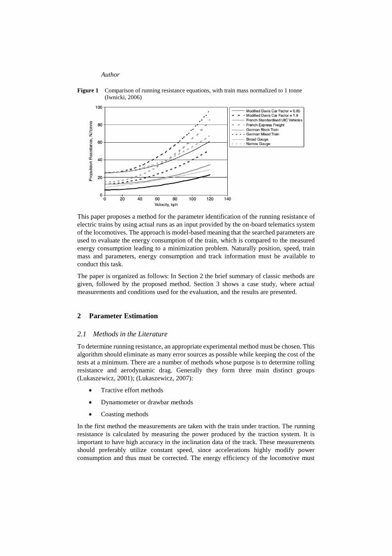
Although there exist many parameters and equations for the running resistance of
longitudinal train dynamics (see Figure 1 and Table 1), the identification of actual
parameters for a chosen locomotive should be beneficial.
Table 1 Empirical Formulas for Running resistance, Freight Rolling stock (Iwnicki, 2006)
Description Equation
Modified Davis equation (U.S.A.) Ka[2.943+89.2/ma+0.0306v+1.741kadv2/(man)]
French Locomotives 0.65 man +13n+0.01 man +0.03 v2
French Standard UIC vehicles g(1.25+ v2/6300)
French Express Freight g(1.5+ v2/(2000…2400))
French 10 tonne/axle g(1.5+ v2/1600)
French 18 tonne/axle g(1.2 v2/4000)
German Strahl formula 25+k(v+Δv)/10k
Broad gauge (i.e., 1.676 m) g[0.87+0.0103v+0.000056 v2]
Broad gauge (i.e., ,1.0 m) g[2.6+0.0003 v2]
Ka is an adjustment factor depending on the rolling stock type; kad is an air drag constant
depending on the car type; ma is mass supported per axle in tonnes; n is the number of
axles; v is the velocity in kilometres per hour; and Δv is the head wind speed, usually taken
as 15 km/h.
Author
Figure 1 Comparison of running resistance equations, with train mass normalized to 1 tonne
(Iwnicki, 2006)
This paper proposes a method for the parameter identification of the running resistance of
electric trains by using actual runs as an input provided by the on-board telematics system
of the locomotives. The approach is model-based meaning that the searched parameters are
used to evaluate the energy consumption of the train, which is compared to the measured
energy consumption leading to a minimization problem. Naturally position, speed, train
mass and parameters, energy consumption and track information must be available to
conduct this task.
The paper is organized as follows: In Section 2 the brief summary of classic methods are
given, followed by the proposed method. Section 3 shows a case study, where actual
measurements and conditions used for the evaluation, and the results are presented.
2 Parameter Estimation
2.1 Methods in the Literature
To determine running resistance, an appropriate experimental method must be chosen. This
algorithm should eliminate as many error sources as possible while keeping the cost of the
tests at a minimum. There are a number of methods whose purpose is to determine rolling
resistance and aerodynamic drag. Generally they form three main distinct groups
(Lukaszewicz, 2001); (Lukaszewicz, 2007):
Tractive effort methods
Dynamometer or drawbar methods
Coasting methods
In the first method the measurements are taken with the train under traction. The running
resistance is calculated by measuring the power produced by the traction system. It is
important to have high accuracy in the inclination data of the track. These measurements
should preferably utilize constant speed, since accelerations highly modify power
consumption and thus must be corrected. The energy efficiency of the locomotive must

Title
also be taken into consideration. Another option is to measure the torque transferred to the
wheel rims by strain gauges, which eliminates the need for the efficiency estimation of the
engine.
To measure the resistance of only the rolling stock, or the internal losses of a tractive unit
the second method utilizes a dynamo-meter, placed between a winch and a cable connected
to the train or vehicle. By pulling the train smoothly on a straight track with constant
gradient the examined parameters could be obtained. In this case, acceleration and
retardation must also be measured and compensated for. Naturally in this way only rolling
resistance at low speed can be measured. Furthermore this method is generally resource
consuming, and the precision and usability of the information acquired are questionable.
With the utilization of the third method the errors and disturbances in the measurement of
the tractive energy can be eliminated. The test requires a track section with known altitude
gradients. First the train accelerates to a previously defined speed, and when it reaches the
beginning of the section it starts to coast, meaning no tractive or braking effort is applied
afterwards. From the measurement of the speed loss one can calculate the loss of kinetic
energy, which is the sum of the rolling resistance and the potential energy loss or gain
resulting from the inclinations of the track.
2.2 The Proposed Method
The method proposed in this paper assumes the presence of data and information gathered
from the telematics system of the train. The information needed for the algorithm is the
following:
The mass of the train (m), which is the sum of the mass of the locomotive (mloc)
and the rolling stock (mstock);
The number of cars in the train (n);
The longitudinal position (s) and speed (v) of the train;
Track information to obtain altitude information;
The measured energy consumption of the train (Emeas).
The quality of the data is important for the model and the actual data sources will be
presented in the section of the case study, while the effects of parameter uncertainty are
examined in the error analysis section.
According to the research and formulas presented in the previous section the running
resistance is divided into two parts: one for the locomotive ( loc
resF ) and one for the rolling
stock ( stock
resF ). The parameters are specifically defined for a particular wagon and
locomotive type, thus the formula of the resistance forces can be formed as:
2( ) *loc loc
res l l lF v Nv m v (2)
2( ) * *stock stock stock
res s s sF v v Nm n v , (3)
where αl,βl,γl are the parameters of the locomotive’s running resistance and αs,βs,γs are the
coefficients of the resistance equation of the rolling stock. The overall running resistance
of the train is the sum of these two forces:

Author
( ) ( ) ( )loc stock
res res resF v F v F Nv (4)
To determine these parameters based on the measurements having one second sample time,
some simplifying assumptions have been made:
Track slope and acceleration are considered as constant for the one-second
sample. Since the dynamics of the railways is slow, this assumption is a minor
simplification.
The model is constructed in such a way that the measured energy consumption is
used in the same sampling time interval. This simplification may cause deviations
since the inner delays in the power and transmission are greater than the sample
time. The rate how the delays in energy measurement affect the identified
parameters will be examined in the error analysis section.
Parameter estimation is carried out by modelling the energy balance of the train in each
sample time, which consists of kinetic- and potential energy and the work generated by the
resistance force. Only the parameters, which are known, are considered in the parameter
estimation. Rotary inertia and the unmeasured external effects, such as wind are omitted in
the model, however, later they will be considered under the efficiency parameter ψj.
Without disturbances and uncertainties the energy consumption of the jth train in the ith
sample is the following:
2 2
, , ( 1), , , , ,
1( )
2i j j i j i j i j j res i j i jE m v v h m Jg F s , (5)
where ,i jE is the energy balance of the sample without considering efficiency and
undetermined effects, Δhi,j is the altitude change and Δsi,j is the length of the inspected
section. The accurate mass of the train must be considered as an uncertain parameter since
it is given as a result of the train composition process. The mass of the jth locomotive (loc
jm
) is known, thus the uncertainty of the mass must be considered with a multiplicative
parameter ( j ) for the rolling stock of each train therefore the real considered mass of the
units after the locomotive is:
stock loc
j j j jm m m kg , (6)
where ξj is the mass uncertainty of the whole train, which has the value range of [0.9, 1.1].
Mechanical efficiency is considered when the energy balance is positive, thus the
locomotive needs additional tractive effort:
, i, j
,
if E 0ˆ0 otherwise
j i j
i j
EE J
(7)
where ψj is the constant aggregated efficiency of the train during the entire run with the
value range of [0.0, 1.0] and so ,
ˆi jE is the estimated energy consumption. The vector of
unknown parameters is formed as:
[ , , , , , , , ]; [1.. ]l l l s s s j jx j k , (8)

Title
where k is the number of individual trains.
By using equations (2)-(7) one can calculate the consumed energy of the trains, when the
parameters (x) are given. To find these parameters, it is necessary to define an objective
function to evaluate their suitability. The simplest approach is to determine the sum of
square differences of calculated and measured consumption in all sample sections:
2
, ,
1 1
ˆ( )jlk
meas
i j i j
j i
g x E E
, (9)
where lj is the number of samples of the jth train, and ,
meas
i jE is the measured energy
consumption. However, this kind of objective function would enlarge the errors caused by
neglecting the actuation delay. Another approach may be the comparison of the cumulated
energy consumption:
2
, ,
1 1
ˆ( )jlk
meas
i j i j
j i
f x
, (10)
where ,i j is the measured and ,ˆi j is the calculated cumulated energy consumption of the
jth train till the ith sample:
, ,
1
i
i j i j
h
E
(11)
According to the equations above, the optimum search problem of the parameter estimation
of the running resistance of the train with the given measurements can be formalized as:
minimize ( )
with respect to [ , , , , , , , ]; 1, ,
subject to 0.9 1.1
0.0 1.0
0.0; 1, ,6
x
l l l s s s j j
j
j
i
f x
x j k
x i
(12)
3 Case Study
3.1 Measurements and Conditions
As mentioned in the previous section, the identification of the parameters of the running
resistance equation is needed for the calculation of energy consumption of the train. The
proposed method used for the parameter identification could be classified into the first
method group with some special additions.
As an illustration of the algorithm, freight rolling stock with the Hungarian State Railways'
0431 series locomotive (formerly named as V43) was used. Table 2 shows the most
important parameters of the locomotive.

Author
Table 2 Main properties of the 0431(V43) locomotive
Power type Electric locomotive (25kV 50Hz AC)
Builder Ganz
Build date 1963-1982
Total produced 379
UIC classification B’B’
Gauge 1.435mm (Standard)
Length 15700 mm
Locomotive weight 80 t
Traction motors 2
Top speed 120 km/h
Power output 2200 kW
In order to perform parameter estimation some fundamental information must be known
about the circumstances and conditions of the investigated runs.
The locomotive on-board computer registers primary voltage, current and phase in one-
second intervals. Thus real power usage can be calculated with the well-known formula by
multiplying voltage, current and the cosine of the phase. The overall error of the power
measurement is approximately 2%.
Position is given in WGS84 (World Geodetic System) coordinates by the Global
Positioning System, and speed is given from two sources, from the GPS device and from
the locomotive’s speedometer with both recorded by the telematics system. GPS speed and
position are provided by a SirfStar 3 GPS chipset keeping the position accuracy below 15
meters and the speed accuracy below 0.1 knots (0.051 m/s) with 95% confidence.
Unfortunately the wheel speed meter, which is an older electromechanical TELOC model
from Hasler Rail has an error of 5% in speed measurement and so can not be used for direct
measurement, only for the refining of the data acquisition delay of the GPS speed signal,
which is below 2 seconds without this correction. According to these data and knowing
some characteristic points of the track, the error of the longitudinal position calculations
may be kept under 0.1%. This low error level in the data is essential, since they must be
synchronized with the altitude diagram of the track, which is given as a function of the
longitudinal distance on the line. Naturally speed measurements could be improved with
more accurate chipsets and position can be refined by using differential GPS. The effect of
position and speed error will be evaluated in the error analysis section.

Title
Figure 2 Line 1 of the Hungarian State Railways. Section between Budapest-Kelenföld and
Tatabánya
The source of the track data is the infrastructure manager of the railways. This means that
the data quality is high although it is impossible to determine its exact accuracy. The
altitude diagram of the 60-km-long section used for the process, the speed trajectory of the
trains, the energy consumption and the calculated tractive forces are shown in Figure 3 and
Figure 4, while the basic parameters are in Table 3.
Figure 3 Track elevation, speed trajectory of sample runs used for parameter estimation
All tractive units and rolling stock are of the same type, although there are uncertainties
and unknown disturbances in these measurements. One is that the gross mass of the trains
is given as a result of cargo mass calculation and can contain 5-10% error. The strength
and direction of the wind are unknown, and the mechanical condition of the wagons, rims
and the locomotive are also unknown, therefore, the parameter identification should
consider these phenomena as an error factor in mass and in other parameters as a certain
kind of cumulated efficiency parameter.

Author
Figure 4 Energy consumption and calculated tractive force of sample runs used for parameter
estimation
Table 3 Basic parameters of the example trains
Running
Time
Gross mass
(t)
Wagon
Count
Wagon
mass (t)
Energy consumtpion
(kWh)
48’30" 557 24 20 893
47’10" 510 19 22 694
45’31" 644 11 51 835
44’30" 1243 19 61 1208
45’40" 882 17 47 1104
3.2 Results
The optimization problem has only linear equality and inequality constraints, although the
objective function given is continuous nonlinear. By choosing any appropriate minimum
search algorithm, such as sequential quadratic programming, trust region reflective or
interior point methods, parameters can be determined. On the example set, the actual
coefficients of the resistance functions are shown in equations (13), (14).
2( ) 0.0121 0.0000409loc loc
res NF v m v (13)
2( ) 0.0187 *1.1400stock stock stock
resF Nv m n v (14)
It can be seen that the optimum search eliminated the linear part of equations (2) and (3),
which is in compliance with most of the previously published formulas.
Figure 5 shows the comparison of the measured and calculated tractive forces for Train
No. 1 and Train No. 2. Unknown disturbances and the effect of the delay can be examined
on these sample diagrams. Figure 6 presents the speed profile and the comparison of
cumulated energy consumption through the example of Train No. 4 and Train No. 5.

Title
Figure 5 Calculated (from measurement) and simulated (with the found parameters) tractive
forces of Train No.1 and Train No. 2
Figure 6 Measured and simulated cumulative energy consumption of Train No.4 and Train No. 5
4 Error analysis
The quality of the output of the algorithm may depend on the quality of the data provided
by the telematics system. Speed and position measurements, energy consumption or the
available track information all may contain errors as it has already been mentioned above.
The real question is how sensitive the method is to the errors provided by the onboard
measurement system.
Since the algorithm uses numerical optimization, an analytic evaluation of error sensitivity
is impossible. Even so it is important to know the correctness of the results given by the
method. For this task, the measurement data of the case study presented above was altered
to simulate different measurement error scenarios. To demonstrate this, three different
scenarios were outlined:
1. Error in the provided track data
2. Error in the measurement of energy consumption
3. Measurement delays
In the first scenario the effect of the inaccuracy in the altitude diagram was examined. For
this task one hundred different altitude diagrams were created with the following rules: The
long term altitude error – taking the 110 m altitude as base – should not exceed 4%, while
the local gradient error should not exceed 10%. The lower and upper bounds of the

Author
generated diagrams can be examined in Figure 7. The figure also presents the acquired
resistance diagrams.
Figure 7 Bounds of the altered altitude diagram, and the identified speed resistance diagrams
generated with the parameters of Train No.1
To simulate the inaccuracy in the measurement of the energy consumption the original
measurements applied in the case study were altered with a similar rule set to the one
described above. The long term error in the energy consumption was kept under 4% and
the local gradient error was kept under 10%.
Then with the one hundred generated energy consumption samples the determination of
the parameters was also carried out. Sample upper and lower bounds of the altered energy
consumption diagram can be examined in Figure 8. The different resistance diagrams
generated as the result of the altered consumption measurements can also be examined in
the figure.
Figure 8 Bounds of the altered energy consumption diagram of Train No.1, and the identified
speed resistance diagrams generated with the parameters of Train No.1
For the emulation of the measurement delays or the asynchronous recordings of the energy
consumption and speed/position values, these two sources were shifted in time from -3
seconds to +3 seconds with 0.5 second steps. The resulting resistance diagrams are shown
in Figure 9.

Title
Figure 9 Resistance diagrams of Train No. 1 with asynchronous data recordings
The summary of the resuts of the error analysis can be seen in Table 4. The generated
running resistance diagrams were compared to the result of the case study at different
speeds taking the train parameters of Train No. 1 as a basis. The three error scenarios were
designed to be at least two times worse than the expected error rate. Based on the results
of the error analysis the following conclusions can be drawn:
Regarding sensitivity the algorithm showed the worst relative performance at low train
speed and the best error suppression was found between 60-80 km/h values. This
phenomemon can be explained with the nature of the applied data set. Since more than
80% of the data had a speed value between 60 and 90 km/h the optimization algorithm
achievied the minimum of the f(x) fitness function by optimizing the curve to this speed
interval. The increasing relative error at higher speed (120 km/h) can be explained the same
way.
Table 4 Results of the error analysis. The maximum of the absolute and relative error of the
generated running resistance diagrams at different speeds (Train No. 1)
Speed (km/h) Error Scenarios
Altitude Performance Delay
0 1.22 kN (11.2%) 1.39 kN (12.8%) 1.32 kN (12.1%)
60 0.60 kN (3.1%) 0.97 kN (5.0%) 0.21 kN (1.1%)
120 2.99 kN (6.7%) 2.05 kN (4.6%) 2.32 kN (5.2%)
5 Conclusions
Running resistance depends on many different parameters of the train or its environment.
However, in several cases the utilization of a simplified model could be expedient because
of its low computational requirements. These models are generally in a form of a second
order polynomial and originated from the Davis equation. Such application area can be the
optimal trajectory planning of the movement of trains. These methods consider speed
limits, track inclinations, train characteristics and resistance forces for the calculation of
optimal speed profiles of the train for given journey times. Moreover, these methods are
sensitive to the appropriate model of the running resistance.
The paper has proposed a method to identify the parameters of the simplified running
resistance formula for different types of trains by utilizing telemetric data that are available

Author
for almost all railway companies. The method can determine the parameters of the formula
from historical data in an offline way. Since the method considers the inclinations of the
railway tracks any runs recorded can be used for the evaluation of the parameters in contrast
with the classic methods that need tracks with constant grades or special test cases.
A case study with the Hungarian V43 type locomotive and freight rolling stock is
presented, which shows the results of the algorithm for one specific case on a track section
with varying inclinations. Since the quality of the output of the algorithm may depend on
the quality of the data provided by the telematics system, an error analysis was conducted
by altering the original measurements to inspect the effect of their error on the resulting
resistance diagram. The results have shown that though the algorithm does not eliminate
measurement errors, the absolute error is kept in an acceptable rate even with the doubling
of the error limit of the specific measurements.
References
Aradi, S., Becsi, T. & Gaspar, P., 2013. A predictive optimization method for energy-
optimal speed profile generation for trains. Budapest, 2013 IEEE 14th International
Symposium on Computational Intelligence and Informatics (CINTI).
Boschetti, G. & Mariscotti, A., 2012. Integrated electromechanical simulation of traction
systems: Relevant factors for the analysis and estimation of energy efficiency. hely nélk.,
Electrical Systems for Aircraft, Railway and Ship Propulsion (ESARS).
Bosquet, R., Vandanjon, P., Coiret, A. & Lorino, T., 2013. Model of High-Speed Train
Energy Consumption. hely nélk., International Conference on Railway Engineering and
Management.
Davis, W., 1926. The tractive resistance of electric locomotives and cars. General Electric
Review, 29. kötet.
Hay, W. W., 1961. Railroad Engineering. New York: John Wiley and Sons.
Howlett, P., Pudney, P. & Vu, X., 2009. Local energy minimization in optimal train
control. Automatica, 45. kötet, pp. 2692-2698.
Iwnicki, S., 2006. Handbook of railway vehicle dynamics. hely nélk.:CRC Press.
Liu, R. R. & Golovitcher, I. M., 2003. Energy-efficient operation of rail vehicles.
Transportation Research Part A, 37. kötet, pp. 917-932.
Lukaszewicz, P., 2001. Energy consumption and running time for trains : modelling of
running resistance and driver behaviour based on full scale testing. hely nélk.:Ph.D.
dissertation.
Lukaszewicz, P., 2007. A simple method to determine train running resistance from full-
scale measurements. hely nélk., Proceedings of the I MECH E Part F Journal of Rail and
Rapid Transit.
Profillidis, V., 2000. Railway engineering. Cambridge: University Press.
Rochard, B. P. & Schmid, F., 2000. A review of methods to measure and calculate train
resistances. hely nélk., Institution of Mechanical Engineers, Part F: Journal of Rail and
Rapid Transit.

Title
Nomenclature
WGS84 World Geodetic System
GPS Global Positioning System.
i,jΔE Energy change during the sample [J]
i,jˆΔE Energy consumption during the sample [J]
meas
i,jΔE Measured energy consumption [J]
i,jε Cumulated energy consumption till the ith sample [J]
loc
resF Running resistance of the locomotive [N]
resFstock Running resistance of the rolling stock [N]
Fres Running Resistance [N]
g The gravity of Earth [9.81 m/s2]
Δhi,j Altitude change of the track at the inspected sample [m]
i Indexer of samples
j Indexer of trains
Ka Adjustment factor depending on the rolling stock type
kad Air drag constant depending on the car type
ma Mass supported per axle [t]
m Train gross mass [kg]
mloc Mass of the locomotive [kg]
mstock Gross mass of the rolling stock [kg]
n Number of axles
nstock Number of wagons
Δsi,j Length of the inspected sample [m]
v Longitudinal train speed [m/s]
Δv Head wind speed, usually taken as 15 km/h.
α,β,γ Coefficients of the generic running resistance formula
αl,βl,γl Coefficients of the resistance formula of the locomotive
αs,βs,γs Coefficients of the resistance formula of the rolling stock
ξj Multiplicative uncertainty of the mass of the train
ψj Overall efficiency and uncertainty of the train