Takings and Tax Revenue: Fiscal Impacts

of Eminent Domain

Carrie B. Kerekes and Dean Stansel

October 2014

MERCATUS WORKING PAPER

All studies in the Mercatus Working Paper series have followed a rigorous process of academic evaluation, including (except where otherwise noted) a double-blind peer review.

Working Papers are intended for further publication in an academic journal. The opinions expressed in Mercatus Working Papers are the authors’ and do not represent official positions of

the Mercatus Center or George Mason University.

2

Carrie B. Kerekes and Dean Stansel. “Takings and Tax Revenue: Fiscal Impacts of Eminent Domain.” Mercatus Working Paper, Mercatus Center at George Mason University, Arlington, VA, October 2014. http://mercatus.org/publication/takings-and-tax-revenue-fiscal-impacts -eminent-domain. Abstract This paper provides the first examination of the relationship between eminent domain activity and the growth (and level) of state and local revenue. We restrict our attention to takings that are for private use, such as the one that led to the landmark Kelo decision in 2005. One of the arguments used by the proponents of such takings is that they will lead to higher levels of tax revenue for state and local governments. Using data on the number of takings for private use, we find virtually no evidence of a positive relationship between eminent domain activity and the level of state and local tax revenue. We find some limited evidence of a negative relationship between eminent domain and future revenue growth. These findings are robust to a variety of model specifications. They have important implications for contemporary public policy debates on this issue. JEL codes: K11, H7, R5 Keywords: eminent domain, state and local tax revenue Author Affiliation and Contact Information Carrie B. Kerekes Associate Professor of Economics Lutgert College of Business, Florida Gulf Coast University ckerekes@fgcu.edu Dean Stansel Associate Professor of Economics Lutgert College of Business, Florida Gulf Coast University dstansel@fgcu.edu

3

Takings and Tax Revenue: Fiscal Impacts of Eminent Domain

Carrie B. Kerekes and Dean Stansel

1. Introduction

The United States Supreme Court decision in Kelo v. City of New London1 in 2005 sparked

outrage around the country. In this decision, the US Supreme Court allowed the use of eminent

domain to transfer property in New London, Connecticut, for private benefit, not for public use

as set forth in the takings clause of the US Constitution. This case focused the attention of

citizens, politicians, and academics on property takings. The general public expressed concern

that homes, churches, or other properties can now be expropriated on the grounds that

redevelopment could decrease unemployment and increase government tax revenue.

Many regarded the Kelo decision as an abuse of government power and a threat to liberty

(Benson 2010; C. Cohen 2006; Lopez, Kerekes, and Johnson 2007). Politicians scurried to

reassure troubled voters by examining, and in some cases modifying, state constitutional

constraints on the use of eminent domain. Academics published articles that chronicled eminent

domain abuse (Berliner 2006), scrutinized state takings for private benefit (Kerekes 2011; Lanza

et al. 2013), and analyzed state reforms in the wake of the Kelo decision (Lopez, Jewel, and

Campbell 2009; Lopez and Totah 2007; Sandefur 2006a; Somin 2007, 2009).

This paper is an extension of a study that emerged from this literature. Turnbull and

Salvino (2009) were the first to empirically examine the relationship between eminent domain

for private benefit and the size of state and local public sectors. The purpose of their paper was to

test the Leviathan hypothesis proposed by Brennan and Buchanan (1980). This argument states

that broader eminent domain powers (i.e., allowing governments to use eminent domain for

1 Kelo et al. v. City of New London, 545 U.S. 469 (2005).

4

redevelopment in order to increase employment or to increase the tax base) provide state and

local governments additional means through which to increase their overall size. In effect, the

2005 decision in Kelo weakened a constitutional constraint on government size. As a result, state

and local public sectors may increase in size.

We utilize the Turnbull and Salvino (2009) model and extend it to investigate the effects

of eminent domain from a different angle. The Kelo ruling allows the compulsory transfer of

property between individuals based on the claim that eminent domain used for redevelopment

results in increases in the tax base that, in turn, convey public benefits.2 Our question is whether

such applications of eminent domain will actually increase revenue. As we discuss below, if

more expansive eminent domain powers undermine the security of private property rights,

eminent domain for private benefit may cause the tax base to shrink as a result of decreases in

private investment. In addition, redevelopment takings may also affect government revenues

through potential increases in rent-seeking behavior. Given the significant potential negative

consequences that arise when government undermines property rights, it is worth investigating

whether eminent domain for development purposes actually generates the additional government

revenue it is purported to create.

Turnbull and Salvino (2009) find that the power to use eminent domain for economic

development is associated with greater government revenue. We build on their work by using a

more precise measure of eminent domain (actual eminent domain activity rather than a binary

variable for potential power), a newer dataset, more control variables, and a new variable for

2 See Brief of the National League of Cities et al. as Amici Curiae Supporting Respondents, Kelo v. City of New London, 545 U.S. 469 (2005) (No. 04-108), available at http://www.communityrights.org/PDFs/Briefs/Kelo.pdf. (“This case is of vital importance to amici, whose members include state and local governments and officials throughout the United States. These officials use eminent domain for many purposes, including as a fundamental tool for economic development in distressed cities like New London. Eminent domain is often indispensable for revitalizing local economies, creating much-needed jobs, and generating revenue that enables cities to provide essential services.”).

5

revenue growth. We find virtually no evidence of a statistically significant positive relationship

between eminent domain and the level of state and local tax revenue. We find limited evidence of a

statistically significant negative relationship between eminent domain and the future growth of state

and local tax revenue. Our failure to find a positive relationship between eminent domain activity

and tax revenues suggests that eminent domain for redevelopment fails to achieve its intended

purpose. Our paper supports arguments for constraints that limit property takings for private gain.

The next section presents the motivation for the paper, including a brief discussion of the

evolution of the interpretation of the takings clause and the general role of property rights.

Section 3 details the empirical model and data. Section 4 provides the econometric results and

Section 5 concludes.

2. Background and Motivation

There is little debate that property rights are a vital component of a market economy. The

institution of well-defined, secure private property rights is the foundation of voluntary

exchange. Property rights provide incentives for individuals to maintain property, seek

opportunities for mutually beneficial trade, and be innovative and entrepreneurial. Property

rights are requisite to coordinate the actions of market participants and generate economic

development (Hayek 1945, 1960; von Mises 1935). The link between secure property rights and

economic growth is well established in the literature on economic development (Acemoglu and

Johnson 2005; Acemoglu, Johnson, and Robinson 2001, 2002; Boettke 1994; Knack and Keefer

1995; Landau 2003; Leblang 1996; Mauro 1995).

When property rights become less secure, individuals are less able to reap the benefits of

a market economy. Individuals are less likely to undertake capital investments as the threat of

6

expropriation of property and physical assets increases (Besley 1995; de Soto 1989, 2000;

Kerekes and Williamson 2008). As incentives for capital accumulation decrease, so too do

incentives for productive entrepreneurship and innovation (Boettke and Coyne 2003; Boettke,

Coyne, and Leeson 2010). Consequently, encroachments on individual property rights—such as

eminent domain activity—undermine economic growth.

2.1. Interpretations of the Takings Clause

While the importance of property rights is not controversial, the use of eminent domain to

acquire property is. The United States government derives its authority to confiscate private

property from the takings clause of the Fifth Amendment to the US Constitution. While the

original intent of the takings clause was that property only be taken for public use and with just

compensation, the interpretation of this clause has changed over time.3 Eminent domain has been

used to take property for public purpose and, increasingly, for private benefit. The traditional

interpretation of public use includes taking private property for the provision of public facilities

and infrastructure, such as railroads, highways, or schools. In such instances, eminent domain

may be used to combat the holdout problem and to reduce the transactions costs associated with

acquiring property for public facilities and infrastructure.

Epstein (1985) provides a comprehensive study of the takings clause and the use of

eminent domain in the United States. The evolution of the utilization of eminent domain for

public use to public purpose and, ultimately, to private benefit, stems from a series of court

cases. Some of the more important cases include Berman v. Parker4 in 1954, Poletown

3 For a more detailed discussion of how the interpretation of the takings clause has changed over time, see Epstein (1985), Greenhut (2004), and Sandefur (2006b). 4 Berman v. Parker, 348 U.S. 26 (1954).

7

Neighborhood Council v. Detroit5 in 1981, and Hawaii Housing Authority v. Midkiff 6 in 1984.

The decision in Berman v. Parker allowed the condemnation of property for the redevelopment

of blighted areas, regardless of whether the land was transferred to other individuals. Detroit was

able to condemn property in a residential neighborhood known as Poletown to provide land for

General Motors Corporation on the basis of the public purpose to reduce unemployment. Finally,

in Hawaii Housing Authority v. Midkiff, Hawaii was permitted to transfer land from landowners

to tenants to reduce the “concentration of land ownership.”

In Kelo v. City of New London, residential property was acquired by eminent domain for

the purpose of redevelopment. The city’s redevelopment plan included a hotel and shopping

center and research, office, and retail space to accompany a new facility for the pharmaceutical

company Pfizer. The city of New London argued that the redevelopment plan fulfilled the public

purpose interpretation of the takings clause because redevelopment would increase employment

and increase the tax base. Kelo relaxed the constraints on the use of eminent domain and implied

that eminent domain can now be used to transfer private property from one private party to

another for private benefit.

This use of eminent domain to seize property for private benefit received significant

attention following Kelo in 2005. Berliner (2003) estimates there were more than 10,282 filed or

threatened condemnations for private use or benefit in the years 1998 through 2002 (or about

2,000 per year across those five years). In the year following the Kelo decision (June 2005 to

June 2006), Berliner (2006) estimates 5,783 properties were condemned or threatened with the

use of eminent domain to benefit other private parties, nearly three times more per year than had

occurred in the 1998–2002 period. 5 Poletown Neighborhood Council v. Detroit, 304 N.W. 2d 455 (1981). 6 Hawaii Housing Authority v. Midkiff, 467 U.S. 229 (1984).

8

2.2. Holdouts, Rent-Seeking, and Investment

Some claim, and the US Supreme Court concurred, that eminent domain for private development

purposes can promote economic growth (Ranis 2007). The argument is that areas that undergo

redevelopment experience increases in employment, home ownership, property values, and tax

revenues. However, Carpenter and Ross (2008) examine the effects of state reforms restricting

eminent domain following the Kelo decision on construction jobs, building permits, and property

tax revenues. They find no evidence that limiting eminent domain for private use negatively

affects these variables. Turnbull, Salvino, and Tasto (2013) examine the relationship between

eminent domain and private-sector employment growth. Their findings indicate that the power to

use eminent domain for economic development does not increase private-sector employment; in

fact, it may actually be associated with slower employment growth.

The previous section emphasized the importance of secure, well-defined property rights

for economic development. In an examination of the abuses of eminent domain, Greenhut

(2004) attributes the prosperity of the United States to secure property rights that create

incentives for investment. Lopez (2010) examines property takings in developed and

developing countries and argues that takings alter incentives to maintain and invest in property

in both contexts. Staley and Blair (2005) present evidence from specific case studies and argue

that eminent domain for development projects has a tendency to be arbitrary and inequitable,

tending to serve private purposes. They argue that eminent domain powers can negatively

impact redevelopment if they make “property rights less certain and investment less

predictable” (Staley and Blair 2005). Eminent domain undermines the security of property

rights, and there is substantial evidence that it also discourages economic growth. Those two

factors undermine the argument for eminent domain’s recently expanded use and provide a

9

rationale for constraining that use by restricting it to instances adhering to the traditional

doctrine on public use.

As previously mentioned, the original intent of the Constitution’s takings clause was that

government could take private property for public use and with just compensation. One of the

primary justifications for eminent domain is to enable the assembly of large tracts of land for

government provision of public facilities and infrastructure (roads, schools, etc.). The argument

is that landowners in these situations have market power and will refrain from selling their

property in order to obtain a higher price. This holdout problem would then make it more

difficult for the government to acquire the property necessary to provide public facilities and

infrastructure (L. Cohen 1991; Merrill 1986).7

Several scholars question the validity of the holdout justification for the use of eminent

domain (Benson 2005; Lopez 2010). Munch (1976) examines property takings and illustrates

that eminent domain is not necessarily more efficient than the private sector at assembling land.

Garrett and Rothstein (2007) demonstrate that takings for private economic development result

in zero-sum games. They argue that eminent domain hampers economic development by

introducing economic inefficiencies.

In a paper challenging the holdout justification for eminent domain, Benson (2005) also

argues that property takings can encourage rent-seeking behavior.8 Tullock (1967) argues that

individuals have an incentive to use the political process to further their own special interests. This

rent-seeking behavior consumes economic resources and imposes costs on an economy that can

7 Epstein (1985) discusses justifications for takings in terms of means and ends. The ends refer to the ultimate purpose of the properties taken by eminent domain; the means refer to how these properties are taken. For example, eminent domain is justified from an ends perspective as it aids government in the provision of public goods. According to the means perspective, eminent domain may be necessary to procure the desired property for a government project (ends). Lanza et al. (2013) provide a summary of the means and ends justifications for eminent domain. 8 For an overview of the rent-seeking literature, see Congleton, Hillman, and Konrad (2008).

10

retard economic growth. Relaxing the constraints on property takings encourages individuals to use

eminent domain to pursue their own ends if such ends are deemed to confer public benefits. Thus,

it opens the door for rent-seeking behavior. Lopez (2010) discusses how interest groups form in

eminent domain cases to try to influence both the outcome and the broader institutional rules that

delineate government powers. For example, local governments, urban planners, and developers

form alliances in support of eminent domain and weaker constraints on government for the purpose

of redevelopment. Property owners, realtors, and some public interest groups align in opposition to

eminent domain and prefer stronger constraints on government powers. Similarly, Boettke, Coyne,

and Leeson (2010) argue that government intervention, including eminent domain and regulatory

takings, promotes unproductive rather than productive entrepreneurship. Rent-seeking activities are

one component of unproductive entrepreneurship (Baumol 1990).9

3. The Data and Empirical Model

Proponents of eminent domain typically argue that it will provide a benefit to the public by

increasing tax revenue10 (which presumably will be used in a way that residents value). This

argument supplies two testable hypotheses:

H1: Eminent domain activity is positively associated with subsequent revenue levels.

H2: Eminent domain activity is positively associated with subsequent revenue growth.

9 Murphy, Shleifer, and Vishny (1993) distinguish between public and private rent-seeking and discuss how rent-seeking is detrimental to economic growth. 10 See Brief of the National League of Cities et al., supra note 2. See also Ranis (2007). “Much has been made recently of Kelo and the negative impact of eminent domain in its use of state and municipal powers to transfer property rights from individual homeowners in poorer, marginal neighborhoods . . . to larger private property enterprises that will achieve simply larger tax revenues. Most eminent domain initiatives are not used to condemn mom-and-pop groceries or small homes for the sake of replacing them with larger operated businesses but rather for large urban, community mixed public and private complexes that provide increased employment, an enhanced tax base, urban development, and community edification” (Ranis 2007, pp. 195–96). “Critical to the impact of Kelo is that it was decided by the Supreme Court on behalf of providing jobs for workers in a depressed area, resurrecting the New London Community, and the important principle of preserving and creating employment and a viable tax base” (p. 203).

11

Using data for 1990 and 2000, Turnbull and Salvino (2009) find that eminent domain for

private benefit is associated with higher levels of tax revenue and own-source revenue as a

percentage of personal income. Their measure of eminent domain is a dummy variable that takes

the value of one for states that explicitly empower local governments to use eminent domain for

private development projects. Only seven states do so. For all the other states, the variable is

given a value of zero. This eminent domain variable does not provide a very precise measure of

the varying levels of eminent domain activity across the states. We build on their work by using

a variable that better captures eminent domain activity across states.

To examine the impact of eminent domain, we use state data on the use of eminent

domain for private benefit from Berliner (2003). Berliner’s data cover the period January 1,

1998, through December 31, 2002. Berliner records the number of total condemnations by state

to indicate the number of properties that have been affected by the use of eminent domain to

benefit private parties.11 Note that the Berliner data understate the total amount of eminent

domain activity as they exclude those activities done for traditional public purposes (schools,

roads, etc.). In a later report, Berliner (2006) provides updated data for the period June 2005

through June 2006, the 12 months following the Kelo Supreme Court decision. These data are

compiled in the same manner as in Berliner’s initial study.

11 Berliner (2003) collects her data from court decisions and published accounts (public documents and news articles). The number of total condemnations for private use or benefit per state is the summation of filed condemnations and threatened condemnations. Filed condemnations record the number of instances for which the government or private parties filed actions in court to transfer private property for private benefit, or local government voted to authorize filing eminent domain action. Threatened condemnations include actions that precede “filing a condemnation action in court or voting to authorize the filing of such action” (Berliner 2006). When a property is threatened with eminent domain the property owner may decide to divest of the property rather than taking action. Therefore, not all threatened cases necessarily result in court filings.

12

We follow Turnbull and Salvino (2009) in measuring tax revenue (and total own-source

revenue)12 as a percentage of personal income and in using three measures: combined state and

local, state only, and local only.13 In addition to the level of revenue, we also examine the growth

of that revenue. To account for the lag between eminent domain activity (over 1998–2002 and

June 2005–June 2006) and subsequent revenue effects, we examine tax revenue levels in 2004

and 2008 and tax revenue growth from 2004 to 2007 and from 2008 to 2011.14 This implies a

minimum of a two-year lag between the eminent domain activity and the revenue effect.

Our independent variable of interest is the eminent domain activity measure described above

for 1998–2002 and June 2005–June 2006. We measure that activity three ways: total condemnations

in the state, total condemnations per total housing units in the state, and total condemnations per

total population in the state. We also use the binary measure of eminent domain power created by

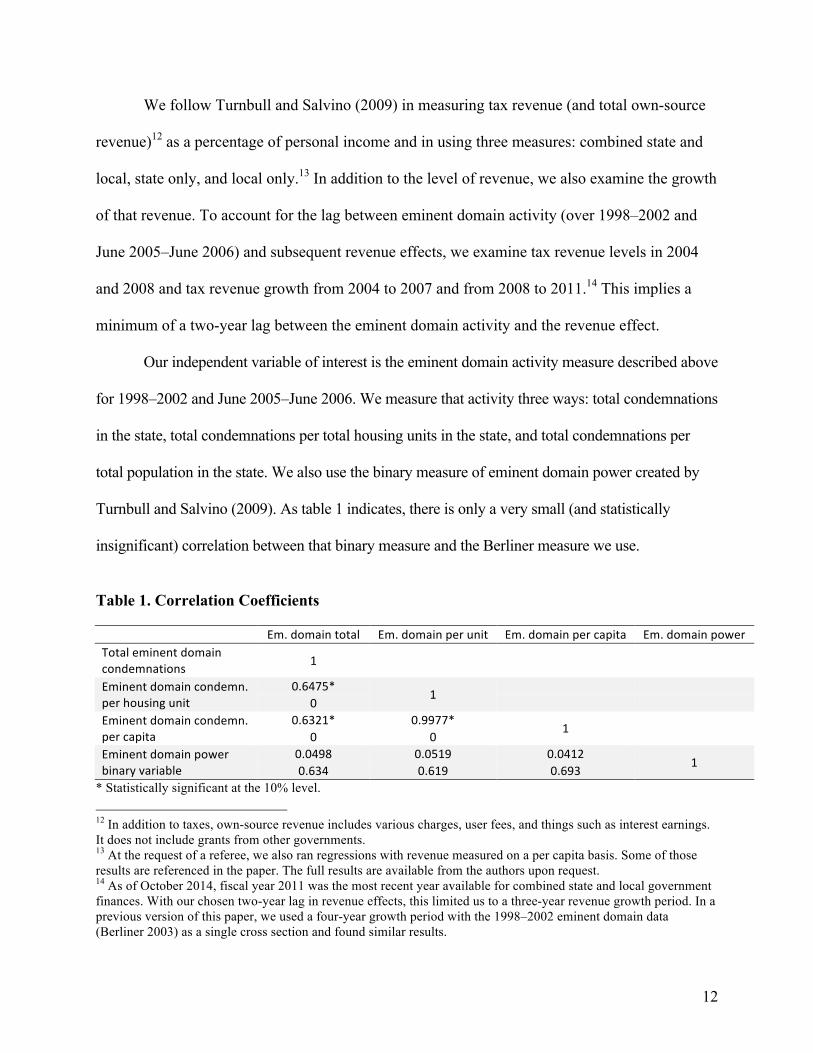
Turnbull and Salvino (2009). As table 1 indicates, there is only a very small (and statistically

insignificant) correlation between that binary measure and the Berliner measure we use.

Table 1. Correlation Coefficients

 Em.  domain  total   Em.  domain  per  unit   Em.  domain  per  capita   Em.  domain  power  

Total  eminent  domain  condemnations   1        

     Eminent  domain  condemn.  per  housing  unit  

0.6475*  1      

0      Eminent  domain  condemn.  per  capita  

0.6321*   0.9977*  1    

0   0    Eminent  domain  power  binary  variable  

0.0498   0.0519   0.0412  1  

0.634   0.619   0.693  * Statistically significant at the 10% level. 12 In addition to taxes, own-source revenue includes various charges, user fees, and things such as interest earnings. It does not include grants from other governments. 13 At the request of a referee, we also ran regressions with revenue measured on a per capita basis. Some of those results are referenced in the paper. The full results are available from the authors upon request. 14 As of October 2014, fiscal year 2011 was the most recent year available for combined state and local government finances. With our chosen two-year lag in revenue effects, this limited us to a three-year revenue growth period. In a previous version of this paper, we used a four-year growth period with the 1998–2002 eminent domain data (Berliner 2003) as a single cross section and found similar results.

13

Following Turnbull and Salvino (2009), we use the same control variables in an attempt

to replicate their results with our new dataset: revenue decentralization (local own-source general

revenue as a percentage of state and local own-source general revenue), expenditure

decentralization (local direct general expenditure as a percentage of state and local direct general

expenditure), state grants to local governments (as a percentage of state expenditure), state

population, urban (metropolitan statistical area or MSA) share of population, median household

income, and a dummy variable for Confederate states. Our initial model is as follows:

(1) Revenuei,t = α + β1Eminent domain activityi,t−2 + β2Fiscal decentralizationi,t + β3Local government counti,t−2 + β4Control variablesi,t.

Then, to expand on Turnbull and Salvino’s work, we enhance their model in a variety of

ways. Instead of using their raw count of the number of local governments to measure

fragmentation,15 we use the number per 100,000 residents to provide more meaningful comparisons

across states with widely differing numbers of residents. We also employ traditional regional

dummy variables rather than their dummy variable for “former Confederate states or border

states.”16 In addition, we add three control variables to account for differences in demographics and

economic conditions that can affect government revenues: the percentage of population aged 18–64,

the unemployment rate, and the real per capita gross domestic product. With few exceptions where

data were unavailable, our data for each of these control variables are for 2004 and 2008 (which are

the two years for which we examine revenue levels and the first year of our two growth periods).

The level and growth of revenue (our dependent variables) may have an impact on

eminent domain activity (our independent variable of interest). For example, governments in

15 Fragmentation refers to the degree to which the local government system is divided into separate jurisdictions. A state with many local governments would be considered to have a highly fragmented system. 16 Because we have a fairly small number of observations (100), we use four regional dummies rather than state fixed effects. The omitted variable is Northeast.

14

states with low or slow-growing revenue may be more likely to utilize eminent domain in order

to increase their revenue. We first address this potential endogeneity problem by including a

control variable for the lagged growth of revenue. To capture the revenue growth trend in each

state, we use 1995–1998 and 2002–2005, the three-year periods before the first year of our

eminent domain activity data for each of the two periods available (1998–2002 and June 2005–

June 2006). Our expanded models are

(2) Revenuei,t = α + β1Eminent domain activityi,t−2 + β2Revenue decentralizationi,t + β3Local governments per 100,000 residentsi,t−2 + β4Control variablesi,t + β5Lagged revenue growthi,t.

(3) Revenue Growthi,t = α + β1Eminent domain activityi,t−2 + β2Revenue decentralizationi,t + β3Local governments per 100,000 residentsi,t−2 + β4Control variablesi,t + β5Lagged revenue growthi,t.

In addition, following Turnbull and Salvino, as an alternative way to address the potential

endogeneity problem, we later drop the lagged revenue growth variable and instead make use of

three instrumental variables for our eminent domain variables: lawyers per 1,000 population,

percentage of land owned by the state government, and income skewness. As Turnbull and

Salvino (2009) suggest, having a higher number of lawyers implies that residents are more likely

to resort to nonmarket solutions to disputes; having a higher percentage of land owned by the

state implies a greater willingness on the part of government to get involved in land markets; and

income skewness “is included to capture possible income distribution effects on choice of

institutional restrictions on local powers” (p. 801).

Data sources are provided in table A1. Summary statistics can be found in table A2.

Correlation coefficients for our three main eminent domain variables and our four main

dependent variables are found in table A3.

15

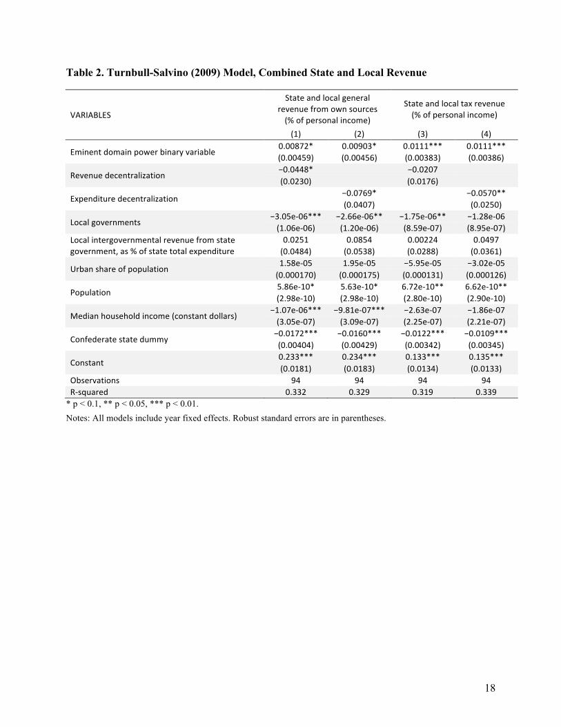
4. Regression Results

We first attempt to replicate the results of Turnbull and Salvino (2009) by utilizing the same

dependent variables and control variables. However, we use revenue data for 2004 and 2008

rather than for 1990 and 2000. Similarly, with two exceptions, each of our control variables is for

2004 and 2008. The first exception is the urban share of population variable, which is only

available for decennial Census years, so we use data for 2000 and an estimate for 2005, achieved

by averaging 2000 and 2010. The second exception is the fragmentation variable, which is only

available for Census of Government years, so we use 2002 and 2007 data. Later, we modify the

Turnbull and Salvino model slightly and add a new dependent variable for revenue growth over

the periods 2004–2007 and 2008–2011.

4.1. Replication of Turnbull and Salvino (2009)

Table 2 shows our results for the combined state and local tax and revenue data, using Turnbull

and Salvino’s binary variable for eminent domain power. As they did, we find evidence of a

statistically significant positive relationship between eminent domain power and the level of

state and local taxes and revenue as a percentage of personal income.17 When we measure

state- and local-level data separately (see table A4), we find that the model’s explanatory

power (measured by the value for R-squared) increases substantially, but the statistically

significant coefficients for the eminent domain power variable only remain for the state

revenue regressions, not for the local revenue regressions. While that insignificance for the

17 When the revenue variables are measured on a per capita basis, the coefficient on the eminent domain power variable is also statistically significant (and positive) in all four of the models. For brevity, those results have not been included. They are available from the authors upon request.

16

local revenue variables contradicts the findings of Turnbull and Salvino, we do consistently

find positive coefficients as they did.18

Next we change how eminent domain is measured. Instead of the binary variable, we use

total condemnations for private purposes. Otherwise, all the other variables are the same. As

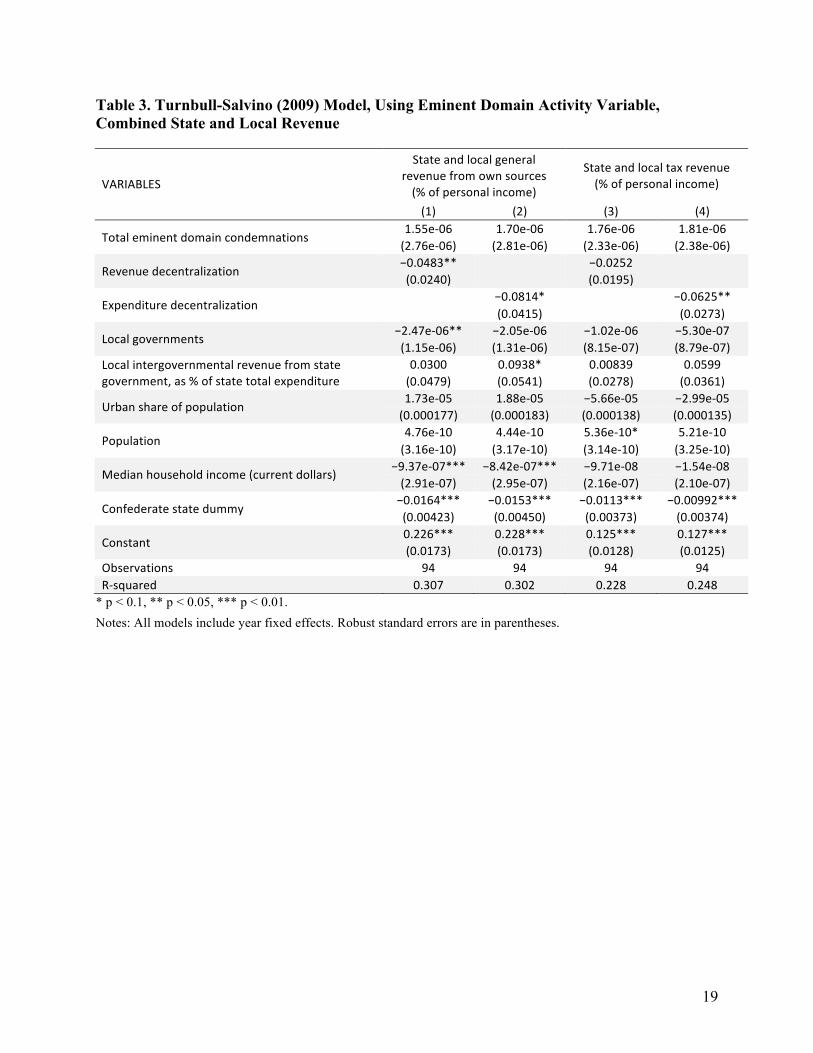
table 3 shows, using this improved measure, we fail to find any statistically significant

relationship between eminent domain activity and revenue levels. (That result holds true when

revenue is measured on a per capita basis as well.) When we measure state and local revenue

data separately, we find similar results—no statistically significant relationship (see table A5).

While the relationships are not significant, we do still find positive coefficients for our more

precise measure of eminent domain activity (with two exceptions, both for local general revenue

from own sources). However, the explanatory power of our models, as indicated by the R-

squared statistic, is slightly lower when we use this more precise measure.

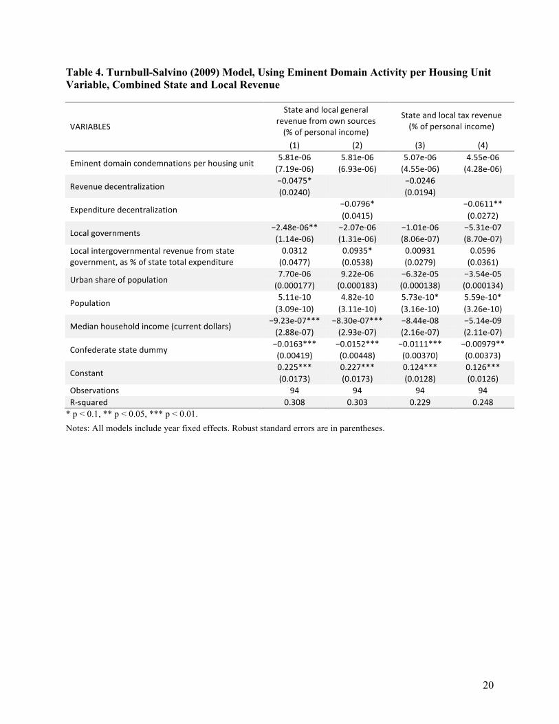
Using the same model, table 4 shows the results when we measure eminent domain

activity as total condemnations per housing unit. Here too we fail to find any statistically

significant relationship between eminent domain activity and revenue levels. Separate results for

state-level data and local-level data are found in table A6. Those results show the same lack of a

statistically significant relationship. (That result holds true when revenue is measured on a per

capita basis as well.) As with the previous set of results, the explanatory power of our models is

slightly lower than with the binary variable for eminent domain.

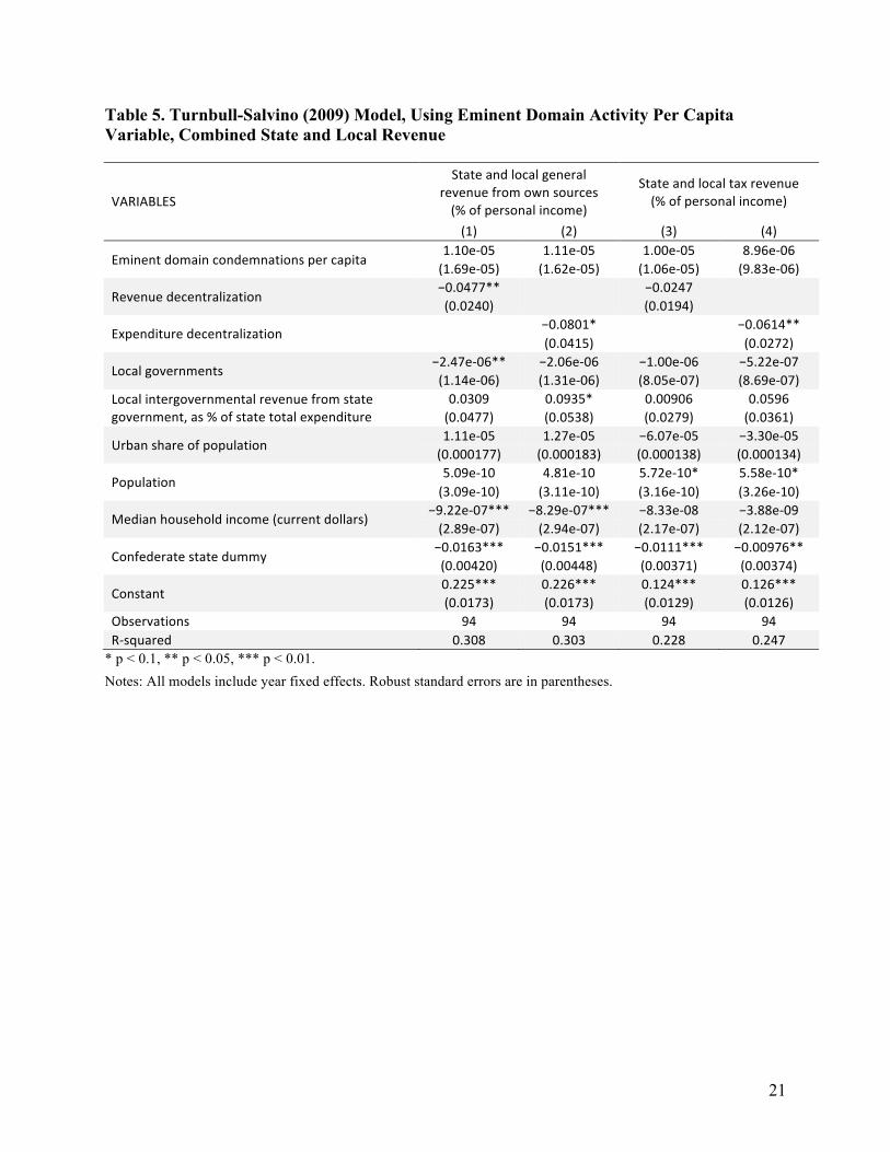
Table 5 shows the results when we measure eminent domain activity as total

condemnations per capita. Otherwise, all the other variables remain the same. Once again, we

find no evidence of a statistically significant relationship between eminent domain activity and 18 When revenue is measured on a per capita basis, the local revenue coefficients remain weakly statistically significant.

17

the level of state and local tax revenue. (That result holds true when revenue is measured on a

per capita basis as well.) Separate results for state-level data and local-level data confirm that

same finding (see table A7).

As tables 2 and A4 show, for eight of our twelve regressions, we confirm the findings of

Turnbull and Salvino (2009) of a statistically significant positive relationship between their

binary measure of eminent domain power and the level of state and local government revenue.

Our results show that their findings are robust to a newer dataset. However, using three different,

more precise measures of eminent domain, we fail to find evidence of a statistically significant

relationship between eminent domain activity and the level of state and local government

revenue. In addition, we find that the explanatory power of our models (measured by the value

for R-squared) is lower when we use our more precise measure of eminent domain activity than

when we use the Turnbull-Salvino binary variable, which provides further support for the idea

that there is no relationship between eminent domain and the level of state and local government

revenue when eminent domain is measured more precisely. These results are robust to changes in

how revenue is measured (own-source general revenue or tax revenue) as well as the level of

government (state and local government revenue combined, state only, and local only), and we

find similar results (not reported herein) when we measure revenue on a per capita basis instead

of as a percentage of personal income.

18

Table 2. Turnbull-Salvino (2009) Model, Combined State and Local Revenue

VARIABLES  

State  and  local  general  revenue  from  own  sources  (%  of  personal  income)  

State  and  local  tax  revenue  (%  of  personal  income)  

(1)   (2)   (3)   (4)  

Eminent  domain  power  binary  variable  0.00872*   0.00903*   0.0111***   0.0111***  (0.00459)   (0.00456)   (0.00383)   (0.00386)  

Revenue  decentralization  −0.0448*  

 −0.0207  

 (0.0230)     (0.0176)    

Expenditure  decentralization     −0.0769*     −0.0570**  

  (0.0407)     (0.0250)  

Local  governments  −3.05e-­‐06***   −2.66e-­‐06**   −1.75e-­‐06**   −1.28e-­‐06  (1.06e-­‐06)   (1.20e-­‐06)   (8.59e-­‐07)   (8.95e-­‐07)  

Local  intergovernmental  revenue  from  state  government,  as  %  of  state  total  expenditure  

0.0251   0.0854   0.00224   0.0497  (0.0484)   (0.0538)   (0.0288)   (0.0361)  

Urban  share  of  population  1.58e-­‐05   1.95e-­‐05   −5.95e-­‐05   −3.02e-­‐05  (0.000170)   (0.000175)   (0.000131)   (0.000126)  

Population  5.86e-­‐10*   5.63e-­‐10*   6.72e-­‐10**   6.62e-­‐10**  (2.98e-­‐10)   (2.98e-­‐10)   (2.80e-­‐10)   (2.90e-­‐10)  

Median  household  income  (constant  dollars)  −1.07e-­‐06***   −9.81e-­‐07***   −2.63e-­‐07   −1.86e-­‐07  (3.05e-­‐07)   (3.09e-­‐07)   (2.25e-­‐07)   (2.21e-­‐07)  

Confederate  state  dummy  −0.0172***   −0.0160***   −0.0122***   −0.0109***  (0.00404)   (0.00429)   (0.00342)   (0.00345)  

Constant  0.233***   0.234***   0.133***   0.135***  (0.0181)   (0.0183)   (0.0134)   (0.0133)  

Observations   94   94   94   94  R-­‐squared   0.332   0.329   0.319   0.339  

* p < 0.1, ** p < 0.05, *** p < 0.01. Notes: All models include year fixed effects. Robust standard errors are in parentheses.

19

Table 3. Turnbull-Salvino (2009) Model, Using Eminent Domain Activity Variable, Combined State and Local Revenue

VARIABLES  

State  and  local  general  revenue  from  own  sources  (%  of  personal  income)  

State  and  local  tax  revenue  (%  of  personal  income)  

(1)   (2)   (3)   (4)  

Total  eminent  domain  condemnations  1.55e-­‐06   1.70e-­‐06   1.76e-­‐06   1.81e-­‐06  (2.76e-­‐06)   (2.81e-­‐06)   (2.33e-­‐06)   (2.38e-­‐06)  

Revenue  decentralization  −0.0483**  

 −0.0252  

 (0.0240)  

 (0.0195)  

 Expenditure  decentralization    

−0.0814*    

−0.0625**  

  (0.0415)     (0.0273)  

Local  governments  −2.47e-­‐06**   −2.05e-­‐06   −1.02e-­‐06   −5.30e-­‐07  (1.15e-­‐06)   (1.31e-­‐06)   (8.15e-­‐07)   (8.79e-­‐07)  

Local  intergovernmental  revenue  from  state  government,  as  %  of  state  total  expenditure  

0.0300   0.0938*   0.00839   0.0599  (0.0479)   (0.0541)   (0.0278)   (0.0361)  

Urban  share  of  population  1.73e-­‐05   1.88e-­‐05   −5.66e-­‐05   −2.99e-­‐05  (0.000177)   (0.000183)   (0.000138)   (0.000135)  

Population  4.76e-­‐10   4.44e-­‐10   5.36e-­‐10*   5.21e-­‐10  (3.16e-­‐10)   (3.17e-­‐10)   (3.14e-­‐10)   (3.25e-­‐10)  

Median  household  income  (current  dollars)  −9.37e-­‐07***   −8.42e-­‐07***   −9.71e-­‐08   −1.54e-­‐08  (2.91e-­‐07)   (2.95e-­‐07)   (2.16e-­‐07)   (2.10e-­‐07)  

Confederate  state  dummy  −0.0164***   −0.0153***   −0.0113***   −0.00992***  (0.00423)   (0.00450)   (0.00373)   (0.00374)  

Constant  0.226***   0.228***   0.125***   0.127***  (0.0173)   (0.0173)   (0.0128)   (0.0125)  

Observations   94   94   94   94  R-­‐squared   0.307   0.302   0.228   0.248  

* p < 0.1, ** p < 0.05, *** p < 0.01. Notes: All models include year fixed effects. Robust standard errors are in parentheses.

20

Table 4. Turnbull-Salvino (2009) Model, Using Eminent Domain Activity per Housing Unit Variable, Combined State and Local Revenue

VARIABLES  

State  and  local  general  revenue  from  own  sources  (%  of  personal  income)  

State  and  local  tax  revenue  (%  of  personal  income)  

(1)   (2)   (3)   (4)  

Eminent  domain  condemnations  per  housing  unit  5.81e-­‐06   5.81e-­‐06   5.07e-­‐06   4.55e-­‐06  (7.19e-­‐06)   (6.93e-­‐06)   (4.55e-­‐06)   (4.28e-­‐06)  

Revenue  decentralization  −0.0475*  

 −0.0246  

 (0.0240)  

 (0.0194)  

 Expenditure  decentralization    

−0.0796*    

−0.0611**  

  (0.0415)     (0.0272)  

Local  governments  −2.48e-­‐06**   −2.07e-­‐06   −1.01e-­‐06   −5.31e-­‐07  (1.14e-­‐06)   (1.31e-­‐06)   (8.06e-­‐07)   (8.70e-­‐07)  

Local  intergovernmental  revenue  from  state  government,  as  %  of  state  total  expenditure  

0.0312   0.0935*   0.00931   0.0596  (0.0477)   (0.0538)   (0.0279)   (0.0361)  

Urban  share  of  population  7.70e-­‐06   9.22e-­‐06   −6.32e-­‐05   −3.54e-­‐05  (0.000177)   (0.000183)   (0.000138)   (0.000134)  

Population  5.11e-­‐10   4.82e-­‐10   5.73e-­‐10*   5.59e-­‐10*  (3.09e-­‐10)   (3.11e-­‐10)   (3.16e-­‐10)   (3.26e-­‐10)  

Median  household  income  (current  dollars)  −9.23e-­‐07***   −8.30e-­‐07***   −8.44e-­‐08   −5.14e-­‐09  (2.88e-­‐07)   (2.93e-­‐07)   (2.16e-­‐07)   (2.11e-­‐07)  

Confederate  state  dummy  −0.0163***   −0.0152***   −0.0111***   −0.00979**  (0.00419)   (0.00448)   (0.00370)   (0.00373)  

Constant  0.225***   0.227***   0.124***   0.126***  (0.0173)   (0.0173)   (0.0128)   (0.0126)  

Observations   94   94   94   94  R-­‐squared   0.308   0.303   0.229   0.248  

* p < 0.1, ** p < 0.05, *** p < 0.01. Notes: All models include year fixed effects. Robust standard errors are in parentheses.

21

Table 5. Turnbull-Salvino (2009) Model, Using Eminent Domain Activity Per Capita Variable, Combined State and Local Revenue

VARIABLES  

State  and  local  general  revenue  from  own  sources  (%  of  personal  income)  

State  and  local  tax  revenue  (%  of  personal  income)  

(1)   (2)   (3)   (4)  

Eminent  domain  condemnations  per  capita  1.10e-­‐05   1.11e-­‐05   1.00e-­‐05   8.96e-­‐06  (1.69e-­‐05)   (1.62e-­‐05)   (1.06e-­‐05)   (9.83e-­‐06)  

Revenue  decentralization  −0.0477**  

 −0.0247  

 (0.0240)  

 (0.0194)  

 Expenditure  decentralization    

−0.0801*    

−0.0614**  

  (0.0415)     (0.0272)  

Local  governments  −2.47e-­‐06**   −2.06e-­‐06   −1.00e-­‐06   −5.22e-­‐07  (1.14e-­‐06)   (1.31e-­‐06)   (8.05e-­‐07)   (8.69e-­‐07)  

Local  intergovernmental  revenue  from  state  government,  as  %  of  state  total  expenditure  

0.0309   0.0935*   0.00906   0.0596  (0.0477)   (0.0538)   (0.0279)   (0.0361)  

Urban  share  of  population  1.11e-­‐05   1.27e-­‐05   −6.07e-­‐05   −3.30e-­‐05  (0.000177)   (0.000183)   (0.000138)   (0.000134)  

Population  5.09e-­‐10   4.81e-­‐10   5.72e-­‐10*   5.58e-­‐10*  (3.09e-­‐10)   (3.11e-­‐10)   (3.16e-­‐10)   (3.26e-­‐10)  

Median  household  income  (current  dollars)  −9.22e-­‐07***   −8.29e-­‐07***   −8.33e-­‐08   −3.88e-­‐09  (2.89e-­‐07)   (2.94e-­‐07)   (2.17e-­‐07)   (2.12e-­‐07)  

Confederate  state  dummy  −0.0163***   −0.0151***   −0.0111***   −0.00976**  (0.00420)   (0.00448)   (0.00371)   (0.00374)  

Constant  0.225***   0.226***   0.124***   0.126***  (0.0173)   (0.0173)   (0.0129)   (0.0126)  

Observations   94   94   94   94  R-­‐squared   0.308   0.303   0.228   0.247  

* p < 0.1, ** p < 0.05, *** p < 0.01. Notes: All models include year fixed effects. Robust standard errors are in parentheses.

22

4.2. New Model

Next, we modify some of the control variables in the Turnbull and Salvino (2009) model and add

four new control variables as well as a new dependent variable for revenue growth. To measure

fragmentation, we use the number of local governments per 100,000 residents instead of

Turnbull and Salvino’s raw count of the number of local governments.19 This provides more

meaningful comparisons across states with widely differing numbers of residents.20 In addition,

rather than their dummy variable for “former Confederate states or border states,” we employ

four traditional regional dummy variables.21 We also add three variables to control for

differences in demographics and economic conditions: the percentage of population aged 18–64,

the unemployment rate, and the per capita GDP.

In the interest of brevity, we drop the total eminent domain condemnations variable, and

we use only one variable for decentralization rather than two. Since the states vary widely in their

population and number of housing units, adjusting the total condemnations data for those two

factors provides a more meaningful comparison across states, so we focus hereafter on the per

housing unit and per capita measures. The two decentralization variables are highly correlated

(with a correlation coefficient of 0.767). Also, they are used independently in separate regressions,

and there are not substantial differences in the results for the eminent domain variables in those

two sets of results (see tables 2–5). We choose to keep the revenue decentralization variable (local

own-source general revenue as a percentage of state and local own-source general revenue) and

drop expenditure decentralization because our focus is on revenue.

19 Stansel (2006) provides an example of this important distinction in previous work in the Leviathan literature. 20 For example, Florida had 1,623 local governments in 2007, nearly two and a half times West Virginia’s 663. By that measure, Florida has substantially greater fragmentation. But Florida has 10 times as many people as West Virginia, so when you adjust for population, Florida is actually substantially less fragmented, not more—8.8 governments per 100,000 people compared to 36.1 in West Virginia. 21 The excluded variable is Northeast.

23

Finally, because there may be a simultaneous relationship between revenue growth and

eminent domain (low or slow-growing revenue may lead states to increase eminent domain

activity), we add a control variable for lagged revenue growth. We use revenue growth over the

periods 1995–1998 and 2002–2005, the three-year periods preceding the first year of our eminent

domain activity data for each period (1998–2002 and June 2005–June 2006).

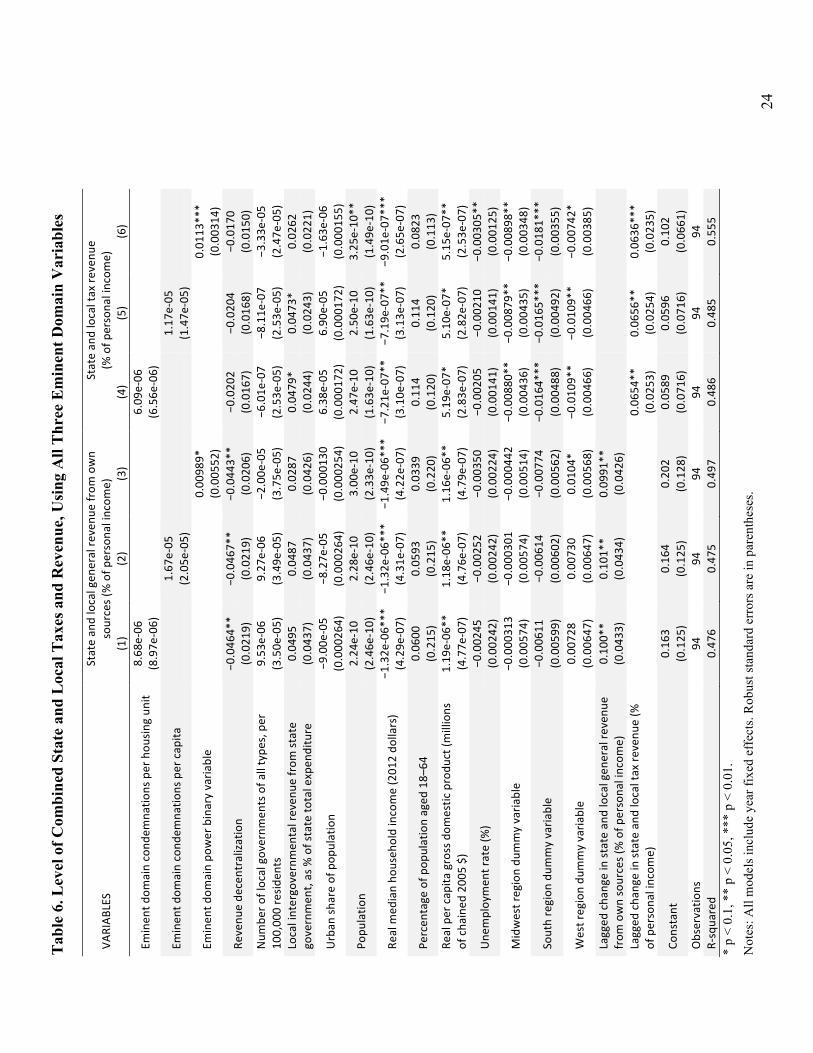
Table 6 shows the results for the level of combined state and local tax and revenue for all

three measures of eminent domain (the binary variable and our two eminent domain activity

variables) when utilizing our revised model. The statistical significance (and the size) of the

coefficients on the eminent domain variables remain roughly the same as with the replications in

the previous section (tables 2–5). The two more precise measures have statistically insignificant

coefficients, and the binary variable continues to have a statistically significant coefficient and

positive sign. Our revised model also consistently provides greater explanatory power. Separate

results for state-level data and local-level data are found in tables A8 and A9. They show the

same basic trends as those described above with the exception that the binary variable is

insignificant in two out of four regressions (both for local government).

24

Tab

le 6

. Lev

el o

f Com

bine

d St

ate

and

Loc

al T

axes

and

Rev

enue

, Usi

ng A

ll T

hree

Em

inen

t Dom

ain

Var

iabl

es

* p

< 0.

1, *

* p

< 0.

05, *

** p

< 0

.01.

N

otes

: All

mod

els i

nclu

de y

ear f

ixed

eff

ects

. Rob

ust s

tand

ard

erro

rs a

re in

par

enth

eses

.

VARIAB

LES  

State  an

d  local  gen

eral  re

venu

e  from

 own  

sources  (%  of  p

ersona

l  incom

e)  

State  an

d  local  tax  re

venu

e  (%

 of  p

ersona

l  incom

e)  

(1)  

(2)  

(3)  

(4)  

(5)  

(6)  

Eminen

t  dom

ain  cond

emna

tions  per  hou

sing  un

it  8.68

e-­‐06

   

 6.09

e-­‐06

   

 (8.97e

-­‐06)  

   

(6.56e

-­‐06)  

   

Eminen

t  dom

ain  cond

emna

tions  per  cap

ita  

 1.67

e-­‐05

   

 1.17

e-­‐05

   

 (2.05e

-­‐05)  

   

(1.47e

-­‐05)  

 Em

inen

t  dom

ain  po

wer  binary  varia

ble  

   

0.00

989*

   

 0.01

13***  

   

(0.005

52)  

   

(0.003

14)  

Revenu

e  de

centralization  

−0.046

4**  

−0.046

7**  

−0.044

3**  

−0.020

2  −0

.020

4  −0

.017

0  (0.021

9)  

(0.021

9)  

(0.020

6)  

(0.016

7)  

(0.016

8)  

(0.015

0)  

Num

ber  o

f  local  governm

ents  of  a

ll  type

s,  per  

100,00

0  resid

ents  

9.53

e-­‐06

 9.27

e-­‐06

 −2

.00e

-­‐05  

−6.01e

-­‐07  

−8.11e

-­‐07  

−3.33e

-­‐05  

(3.50e

-­‐05)  

(3.49e

-­‐05)  

(3.75e

-­‐05)  

(2.53e

-­‐05)  

(2.53e

-­‐05)  

(2.47e

-­‐05)  

Local  intergovernmen

tal  reven

ue  from

 state  

governmen

t,  as  %  of  state  to

tal  expen

diture  

0.04

95  

0.04

87  

0.02

87  

0.04

79*  

0.04

73*  

0.02

62  

(0.043

7)  

(0.043

7)  

(0.042

6)  

(0.024

4)  

(0.024

3)  

(0.022

1)  

Urban

 share  of  pop

ulation  

−9.00e

-­‐05  

−8.27e

-­‐05  

−0.000

130  

6.38

e-­‐05

 6.90

e-­‐05

 −1

.63e

-­‐06  

(0.000

264)  

(0.000

264)  

(0.000

254)  

(0.000

172)  

(0.000

172)  

(0.000

155)  

Popu

latio

n  2.24

e-­‐10

 2.28

e-­‐10

 3.00

e-­‐10

 2.47

e-­‐10

 2.50

e-­‐10

 3.25

e-­‐10

**  

(2.46e

-­‐10)  

(2.46e

-­‐10)  

(2.33e

-­‐10)  

(1.63e

-­‐10)  

(1.63e

-­‐10)  

(1.49e

-­‐10)  

Real  m

edian  ho

useh

old  income  (201

2  do

llars)  

−1.32e

-­‐06*

**  

−1.32e

-­‐06*

**  

−1.49e

-­‐06*

**  

−7.21e

-­‐07*

*  −7

.19e

-­‐07*

*  −9

.01e

-­‐07*

**  

(4.29e

-­‐07)  

(4.31e

-­‐07)  

(4.22e

-­‐07)  

(3.10e

-­‐07)  

(3.13e

-­‐07)  

(2.65e

-­‐07)  

Percen

tage  of  p

opulation  aged

 18–

64  

0.06

00  

0.05

93  

0.03

39  

0.11

4  0.11

4  0.08

23  

(0.215

)  (0.215

)  (0.220

)  (0.120

)  (0.120

)  (0.113

)  Re

al  per  cap

ita  gross  dom

estic  produ

ct  (m

illions  

of  cha

ined

 200

5  $)  

1.19

e-­‐06

**  

1.18

e-­‐06

**  

1.16

e-­‐06

**  

5.19

e-­‐07

*  5.10

e-­‐07

*  5.15

e-­‐07

**  

(4.77e

-­‐07)  

(4.76e

-­‐07)  

(4.79e

-­‐07)  

(2.83e

-­‐07)  

(2.82e

-­‐07)  

(2.53e

-­‐07)  

Une

mploymen

t  rate  (%

)  −0

.002

45  

−0.002

52  

−0.003

50  

−0.002

05  

−0.002

10  

−0.003

05**  

(0.002

42)  

(0.002

42)  

(0.002

24)  

(0.001

41)  

(0.001

41)  

(0.001

25)  

Midwest  region  du

mmy  varia

ble  

−0.000

313  

−0.000

301  

−0.000

442  

−0.008

80**  

−0.008

79**  

−0.008

98**  

(0.005

74)  

(0.005

74)  

(0.005

14)  

(0.004

36)  

(0.004

35)  

(0.003

48)  

South  region

 dum

my  varia

ble  

−0.006

11  

−0.006

14  

−0.007

74  

−0.016

4***  

−0.016

5***  

−0.018

1***  

(0.005

99)  

(0.006

02)  

(0.005

62)  

(0.004

88)  

(0.004

92)  

(0.003

55)  

West  region  du

mmy  varia

ble  

0.00

728  

0.00

730  

0.01

04*  

−0.010

9**  

−0.010

9**  

−0.007

42*  

(0.006

47)  

(0.006

47)  

(0.005

68)  

(0.004

66)  

(0.004

66)  

(0.003

85)  

Lagged

 cha

nge  in  state  an

d  local  gen

eral  re

venu

e  from

 own  sources  (%  of  p

ersona

l  incom

e)  

0.10

0**  

0.10

1**  

0.09

91**  

   

 (0.043

3)  

(0.043

4)  

(0.042

6)  

   

 Lagged

 cha

nge  in  state  an

d  local  tax  re

venu

e  (%

 of  persona

l  incom

e)  

   

 0.06

54**  

0.06

56**  

0.06

36***  

   

 (0.025

3)  

(0.025

4)  

(0.023

5)  

Constant  

0.16

3  0.16

4  0.20

2  0.05

89  

0.05

96  

0.10

2  (0.125

)  (0.125

)  (0.128

)  (0.071

6)  

(0.071

6)  

(0.066

1)  

Observatio

ns  

94  

94  

94  

94  

94  

94  

R-­‐squa

red  

0.47

6  0.47

5  0.49

7  0.48

6  0.48

5  0.55

5  

25

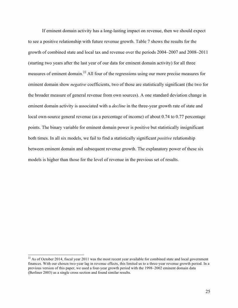
If eminent domain activity has a long-lasting impact on revenue, then we should expect

to see a positive relationship with future revenue growth. Table 7 shows the results for the

growth of combined state and local tax and revenue over the periods 2004–2007 and 2008–2011

(starting two years after the last year of our data for eminent domain activity) for all three

measures of eminent domain.22 All four of the regressions using our more precise measures for

eminent domain show negative coefficients, two of those are statistically significant (the two for

the broader measure of general revenue from own sources). A one standard deviation change in

eminent domain activity is associated with a decline in the three-year growth rate of state and

local own-source general revenue (as a percentage of income) of about 0.74 to 0.77 percentage

points. The binary variable for eminent domain power is positive but statistically insignificant

both times. In all six models, we fail to find a statistically significant positive relationship

between eminent domain and subsequent revenue growth. The explanatory power of these six

models is higher than those for the level of revenue in the previous set of results.

22 As of October 2014, fiscal year 2011 was the most recent year available for combined state and local government finances. With our chosen two-year lag in revenue effects, this limited us to a three-year revenue growth period. In a previous version of this paper, we used a four-year growth period with the 1998–2002 eminent domain data (Berliner 2003) as a single cross section and found similar results.

26

Tab

le 7

. Thr

ee-Y

ear

Gro

wth

of C

ombi

ned

Stat

e an

d L

ocal

Tax

es a

nd R

even

ue, U

sing

All

Thr

ee E

min

ent D

omai

n V

aria

bles

VARIAB

LES  

Chan

ge  in  state  an

d  local  gen

eral  re

venu

e  from

 own  

sources  (%  of  p

ersona

l  incom

e)  

Chan

ge  in  state  an

d  local  tax  re

venu

e  (%

 of  p

ersona

l  incom

e)  

(1)  

(2)  

(3)  

(4)  

(5)  

(6)  

Eminen

t  dom

ain  cond

emna

tions  per  hou

sing  un

it  −5

.03e

-­‐05*

*    

 −3

.92e

-­‐05  

   

(2.40e

-­‐05)  

   

(3.04e

-­‐05)  

   

Eminen

t  dom

ain  cond

emna

tions  per  cap

ita  

 −0

.000

118*

*    

 −9

.26e

-­‐05  

   

(5.36e

-­‐05)  

   

(6.83e

-­‐05)  

 Em

inen

t  dom

ain  po

wer  binary  varia

ble  

   

0.00

126  

   

0.00

231  

   

(0.010

4)  

   

(0.013

5)  

Revenu

e  de

centralization  

−0.060

5  −0

.060

9  −0

.049

9  −0

.096

0  −0

.096

2  −0

.087

3  (0.049

7)  

(0.049

7)  

(0.051

9)  

(0.070

7)  

(0.070

7)  

(0.070

9)  

Num

ber  o

f  local  governm

ents  of  a

ll  type

s,  

per  1

00,000

 resid

ents  

0.00

0177

*  0.00

0176

*  0.00

0187

*  0.00

0402

**  

0.00

0401

**  

0.00

0406

**  

(0.000

104)  

(0.000

104)  

(0.000

111)  

(0.000

185)  

(0.000

185)  

(0.000

188)  

Local  intergovernmen

tal  reven

ue  from

 state  

governmen

t,  as  %  of  state  to

tal  expen

diture  

0.08

63  

0.08

57  

0.11

0  0.12

2  0.12

1  0.13

8  (0.075

8)  

(0.075

9)  

(0.079

4)  

(0.112

)  (0.112

)  (0.112

)  

Urban

 share  of  pop

ulation  

0.00

0319

 0.00

0322

 5.75

e-­‐05

 0.00

0500

 0.00

0503

 0.00

0285

 (0.000

493)  

(0.000

490)  

(0.000

501)  

(0.000

713)  

(0.000

710)  

(0.000

699)  

Popu

latio

n  −1

.61e

-­‐10  

−1.60e

-­‐10  

−2.90e

-­‐10  

3.93

e-­‐10

 3.95

e-­‐10

 3.00

e-­‐10

 (6.53e

-­‐10)  

(6.51e

-­‐10)  

(6.77e

-­‐10)  

(9.17e

-­‐10)  

(9.16e

-­‐10)  

(9.22e

-­‐10)  

Real  m

edian  ho

useh

old  income  (201

2  do

llars)  

6.58

e-­‐07

 6.11

e-­‐07

 7.81

e-­‐07

 8.81

e-­‐07

 8.44

e-­‐07

 9.58

e-­‐07

 (7.49e

-­‐07)  

(7.45e

-­‐07)  

(8.92e

-­‐07)  

(9.82e

-­‐07)  

(9.81e

-­‐07)  

(1.10e

-­‐06)  

Percen

tage  of  p

opulation  aged

 18–

64  

0.60

0  0.60

9  0.57

6  0.82

5  0.83

3  0.80

2  (0.412

)  (0.411

)  (0.408

)  (0.520

)  (0.520

)  (0.513

)  Re

al  per  cap

ita  gross  dom

estic  produ

ct  (m

illions  

of  cha

ined

 200

5  $)  

−5.89e

-­‐07  

−5.90e

-­‐07  

−1.67e

-­‐07  

−1.58e

-­‐07  

−1.60e

-­‐07  

1.79

e-­‐07

 (7.31e

-­‐07)  

(7.23e

-­‐07)  

(7.19e

-­‐07)  

(1.19e

-­‐06)  

(1.19e

-­‐06)  

(1.15e

-­‐06)  

Une

mploymen

t  rate  (%

)  0.00

654  

0.00

641  

0.00

907*

 0.00

862  

0.00

851  

0.01

05  

(0.004

80)  

(0.004

78)  

(0.005

19)  

(0.006

75)  

(0.006

73)  

(0.006

91)  

Midwest  region  du

mmy  varia

ble  

−0.008

81  

−0.008

82  

−0.009

17  

−0.014

3  −0

.014

3  −0

.014

7  (0.012

4)  

(0.012

4)  

(0.012

0)  

(0.016

6)  

(0.016

6)  

(0.016

1)  

South  region

 dum

my  varia

ble  

0.00

907  

0.00

864  

0.01

21  

0.01

56  

0.01

53  

0.01

78  

(0.012

3)  

(0.012

3)  

(0.013

1)  

(0.014

7)  

(0.014

7)  

(0.015

2)  

West  region  du

mmy  varia

ble  

0.00

466  

0.00

473  

0.00

422  

0.00

854  

0.00

861  

0.00

856  

(0.013

3)  

(0.013

3)  

(0.014

1)  

(0.018

5)  

(0.018

5)  

(0.019

0)  

Lagged

 cha

nge  in  state  an

d  local  gen

eral  re

venu

e  from

 own  sources  (%  of  p

ersona

l  incom

e)  

0.11

2***  

0.11

2***  

0.11

2***  

   

 (0.008

42)  

(0.008

41)  

(0.008

64)  

   

 Lagged

 cha

nge  in  state  an

d  local  tax  re

venu

e  (%

 of  persona

l  incom

e)  

   

 0.08

41  

0.08

32  

0.07

96  

   

 (0.115

)  (0.115

)  (0.116

)  

Constant  

−0.502

**  

−0.504

**  

−0.519

**  

−0.719

**  

−0.720

**  

−0.727

**  

(0.250

)  (0.249

)  (0.244

)  (0.314

)  (0.313

)  (0.309

)  Observatio

ns  

94  

94  

94  

94  

94  

94  

R-­‐squa

red  

0.78

2  0.78

3  0.77

2  0.67

4  0.67

5  0.66

9  *

p <

0.1,

**

p <

0.05

, ***

p <

0.0

1.

Not

es: A

ll m

odel

s inc

lude

yea

r fix

ed e

ffec

ts. R

obus

t sta

ndar

d er

rors

are

in p

aren

thes

es.

27

Separate results for state data and local data are found in tables A10 and A11. At the state

level, the four coefficients for our two new eminent domain activity variables are all negative

and statistically significant. For example, a one standard deviation change in eminent domain

activity is associated with a decline in the three-year growth rate of state own-source general

revenue (as a percentage of income) of about 0.94–1.22 percentage points. At the local level, the

four coefficients are all positive, but only the two for the narrower measure of tax revenue

growth are statistically significant. However, the overall explanatory power of all four of those

local models is much lower than for the state government models (R-squareds of about 0.34

versus 0.75 for revenue and about 0.14 versus 0.69 for taxes). In contrast, all four regressions

using the binary variable (eminent domain power) show positive but statistically insignificant

coefficients (just as they were for the combined state and local totals in table 7 above). There too

the local-level regressions have a much smaller R-squared.

In our effort to closely replicate the approach of Turnbull and Salvino (2009), we confirm

their findings of a positive relationship between their binary variable for eminent domain power and

the level of state and local government revenue with a newer dataset. However, those findings are

not robust to the usage of more precise measures of eminent domain. Using those new measures, we

find no evidence of a statistically significant relationship between eminent domain activity and the

level of state and local tax revenue, and thus fail to find support for the hypothesis (H1) that eminent

domain activity is positively associated with the subsequent level of tax revenue. In contrast, our

results for the hypothesis (H2) that eminent domain activity is positively associated with subsequent

state and local government revenue growth are mixed. The binary variable is statistically

insignificant in all four regressions, but six of the eight regressions for our new eminent domain

activity measures are statistically significant, negative four times and positive twice.

28

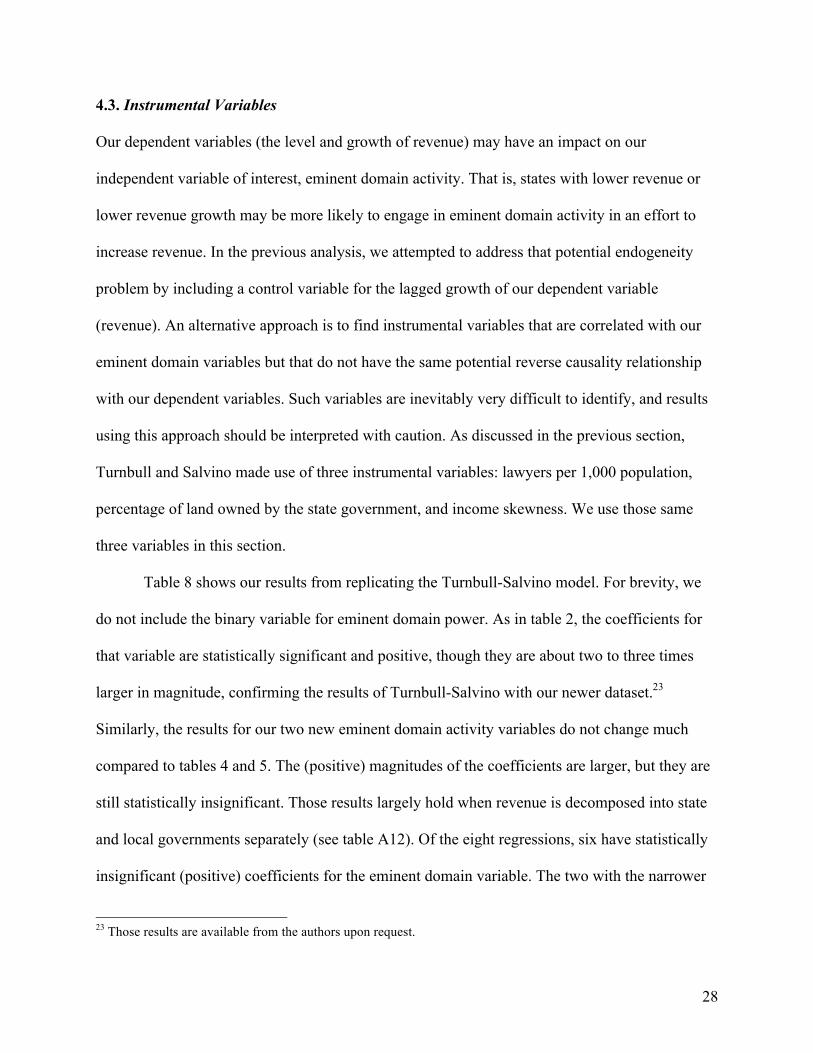
4.3. Instrumental Variables

Our dependent variables (the level and growth of revenue) may have an impact on our

independent variable of interest, eminent domain activity. That is, states with lower revenue or

lower revenue growth may be more likely to engage in eminent domain activity in an effort to

increase revenue. In the previous analysis, we attempted to address that potential endogeneity

problem by including a control variable for the lagged growth of our dependent variable

(revenue). An alternative approach is to find instrumental variables that are correlated with our

eminent domain variables but that do not have the same potential reverse causality relationship

with our dependent variables. Such variables are inevitably very difficult to identify, and results

using this approach should be interpreted with caution. As discussed in the previous section,

Turnbull and Salvino made use of three instrumental variables: lawyers per 1,000 population,

percentage of land owned by the state government, and income skewness. We use those same

three variables in this section.

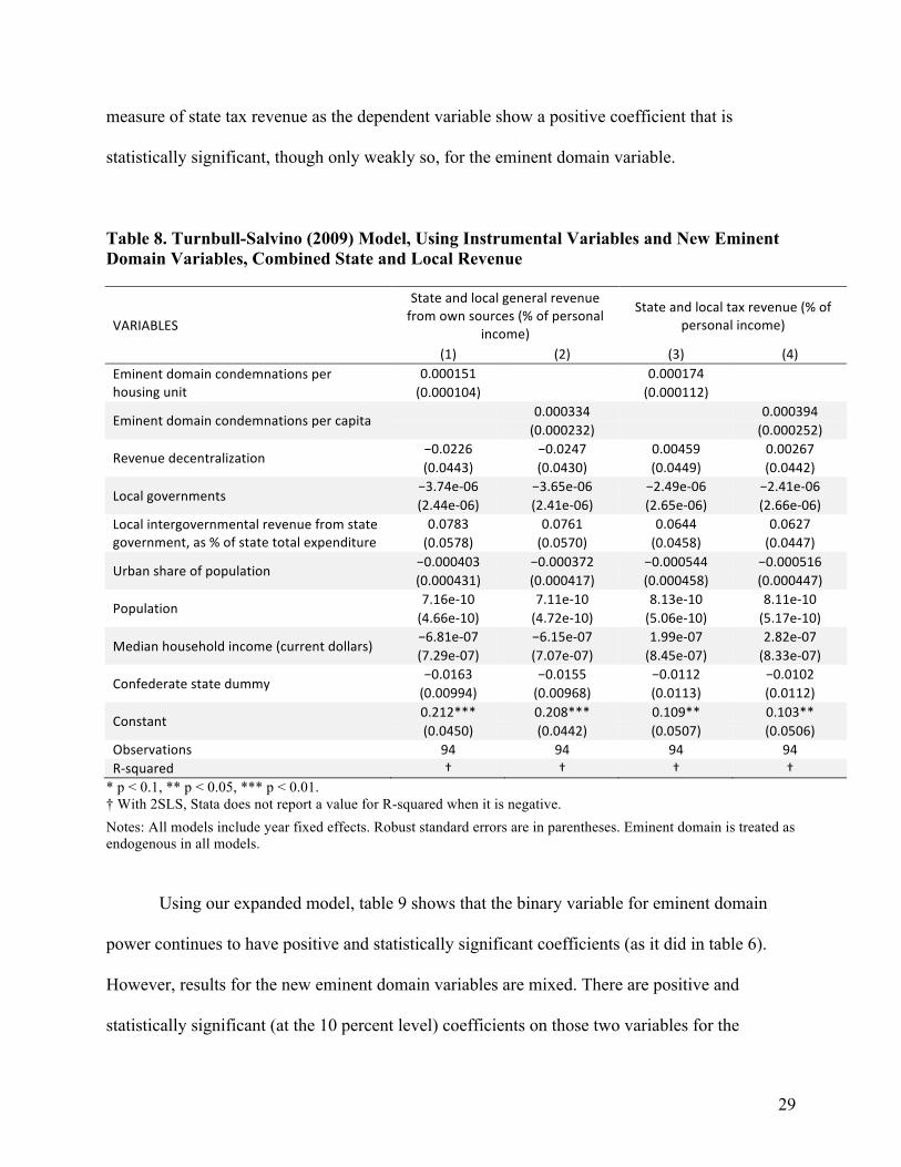
Table 8 shows our results from replicating the Turnbull-Salvino model. For brevity, we

do not include the binary variable for eminent domain power. As in table 2, the coefficients for

that variable are statistically significant and positive, though they are about two to three times

larger in magnitude, confirming the results of Turnbull-Salvino with our newer dataset.23

Similarly, the results for our two new eminent domain activity variables do not change much

compared to tables 4 and 5. The (positive) magnitudes of the coefficients are larger, but they are

still statistically insignificant. Those results largely hold when revenue is decomposed into state

and local governments separately (see table A12). Of the eight regressions, six have statistically

insignificant (positive) coefficients for the eminent domain variable. The two with the narrower

23 Those results are available from the authors upon request.

29

measure of state tax revenue as the dependent variable show a positive coefficient that is

statistically significant, though only weakly so, for the eminent domain variable.

Table 8. Turnbull-Salvino (2009) Model, Using Instrumental Variables and New Eminent Domain Variables, Combined State and Local Revenue

VARIABLES  

State  and  local  general  revenue  from  own  sources  (%  of  personal  

income)  

State  and  local  tax  revenue  (%  of  personal  income)  

(1)   (2)   (3)   (4)  Eminent  domain  condemnations  per    housing  unit  

0.000151    

0.000174    

(0.000104)    

(0.000112)    

Eminent  domain  condemnations  per  capita     0.000334     0.000394  

  (0.000232)     (0.000252)  

Revenue  decentralization  −0.0226   −0.0247   0.00459   0.00267  (0.0443)   (0.0430)   (0.0449)   (0.0442)  

Local  governments  −3.74e-­‐06   −3.65e-­‐06   −2.49e-­‐06   −2.41e-­‐06  (2.44e-­‐06)   (2.41e-­‐06)   (2.65e-­‐06)   (2.66e-­‐06)  

Local  intergovernmental  revenue  from  state  government,  as  %  of  state  total  expenditure  

0.0783   0.0761   0.0644   0.0627  (0.0578)   (0.0570)   (0.0458)   (0.0447)  

Urban  share  of  population  −0.000403   −0.000372   −0.000544   −0.000516  (0.000431)   (0.000417)   (0.000458)   (0.000447)  

Population  7.16e-­‐10   7.11e-­‐10   8.13e-­‐10   8.11e-­‐10  (4.66e-­‐10)   (4.72e-­‐10)   (5.06e-­‐10)   (5.17e-­‐10)  

Median  household  income  (current  dollars)  −6.81e-­‐07   −6.15e-­‐07   1.99e-­‐07   2.82e-­‐07  (7.29e-­‐07)   (7.07e-­‐07)   (8.45e-­‐07)   (8.33e-­‐07)  

Confederate  state  dummy  −0.0163   −0.0155   −0.0112   −0.0102  (0.00994)   (0.00968)   (0.0113)   (0.0112)  

Constant  0.212***   0.208***   0.109**   0.103**  (0.0450)   (0.0442)   (0.0507)   (0.0506)  

Observations   94   94   94   94  R-­‐squared   †   †   †   †  

* p < 0.1, ** p < 0.05, *** p < 0.01. † With 2SLS, Stata does not report a value for R-squared when it is negative. Notes: All models include year fixed effects. Robust standard errors are in parentheses. Eminent domain is treated as endogenous in all models.

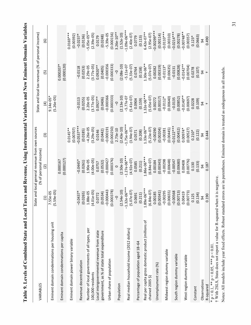
Using our expanded model, table 9 shows that the binary variable for eminent domain

power continues to have positive and statistically significant coefficients (as it did in table 6).

However, results for the new eminent domain variables are mixed. There are positive and

statistically significant (at the 10 percent level) coefficients on those two variables for the

30

narrower measure of tax revenue. However, for the broader measure of general revenue from

own sources, the (positive) coefficients are not statistically significant. As with the more

compact model in table 8 (discussed in the previous paragraph), when revenue is measured

separately for state and local governments (tables A13 and A14), six of the eight coefficients on

our eminent domain variables are statistically insignificant (and positive). Only the two for the

narrower measure of state tax revenue are statistically significant, and only at the 10 percent

level. Three of the four coefficients for the binary variable are significant and positive.

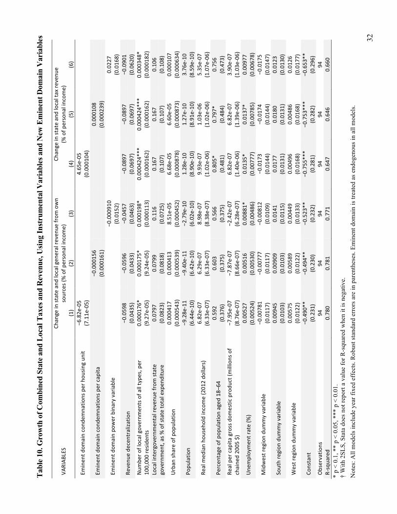
Table 10 shows that our two eminent domain variables have no statistically significant

relationship with the growth of taxes and revenue. This is in contrast to the previous OLS results

in table 7 in which two of the four regressions showed a statistically significant negative

relationship with growth. Neither of the two regressions using the binary variable for eminent

domain power showed a statistically significant relationship either. The results are no different

when revenue is measured separately for state and local governments (tables A15 and A16), with

one exception. In one of the regressions, the binary variable has a statistically significant positive

coefficient (table A16).

31

Tab

le 9

. Lev

els o

f Com

bine

d St

ate

and

Loc

al T

axes

and

Rev

enue

, Usi

ng In

stru

men

tal V

aria

bles

and

New

Em

inen

t Dom

ain

Var

iabl

es

VARIAB

LES  

State  an

d  local  gen

eral  re

venu

e  from

 own  sources  

(%  of  p

ersona

l  incom

e)  

State  an

d  local  tax  re

venu

e  (%

 of  p

ersona

l  incom

e)  

(1)  

(2)  

(3)  

(4)  

(5)  

(6)  

Eminen

t  dom

ain  cond

emna

tions  per  hou

sing  un

it  7.55

e-­‐05

   

 9.14

e-­‐05

*    

 (5.59e

-­‐05)  

   

(5.26e

-­‐05)  

   

Eminen

t  dom

ain  cond

emna

tions  per  cap

ita  

 0.00

0167

   

 0.00

0207

*    

 (0.000

127)  

   

(0.000

120)  

 Em

inen

t  dom

ain  po

wer  binary  varia

ble  

   

0.01

45**  

   

0.01

69***  

   

(0.007

07)  

   

(0.003

92)  

Revenu

e  de

centralization  

−0.043

7*  

−0.044

5*  

−0.053

7***  

−0.011

3  −0

.011

8  −0

.023

7*  

(0.026

5)  

(0.026

1)  

(0.018

5)  

(0.025

5)  

(0.025

3)  

(0.013

6)  

Num

ber  o

f  local  governm

ents  of  a

ll  type

s,  per  

100,00

0  resid

ents  

1.88

e-­‐05

 1.90

e-­‐05

 −4

.26e

-­‐05  

2.20

e-­‐05

 2.29

e-­‐05

 −5

.05e

-­‐05*

*  (4.01e

-­‐05)  

(4.00e

-­‐05)  

(3.29e

-­‐05)  

(3.77e

-­‐05)  

(3.77e

-­‐05)  

(2.39e

-­‐05)  

Local  intergovernmen

tal  reven

ue  from

 state  

governmen

t,  as  %  of  state  to

tal  expen

diture  

0.07

72  

0.07

57  

0.01

46  

0.09

27**  

0.09

20**  

0.01

79  

(0.053

4)  

(0.053

2)  

(0.044

2)  

(0.040

6)  

(0.040

5)  

(0.024

8)  

Urban

 share  of  pop

ulation  

−0.000

443  

−0.000

427  

−0.000

191  

−0.000

366  

−0.000

356  

−5.39e

-­‐05  

(0.000

378)  

(0.000

376)  

(0.000

250)  

(0.000

333)  

(0.000

333)  

(0.000

156)  

Popu

latio

n  −0

 0  

2.73

e-­‐10

 −0

 −0

 3.26

e-­‐10

**  

(2.54e

-­‐10)  

(2.50e

-­‐10)  

(2.43e

-­‐10)  

(2.13e

-­‐10)  

(2.08e

-­‐10)  

(1.52e

-­‐10)  

Real  m

edian  ho

useh

old  income  (201

2  do

llars)  

−1.32e

-­‐06*

**  

−1.27e

-­‐06*

**  

−1.75e

-­‐06*

**  

−5.77e

-­‐07  

−5.11e

-­‐07  

−1.09e

-­‐06*

**  

(5.07e

-­‐07)  

(4.92e

-­‐07)  

(3.94e

-­‐07)  

(5.41e

-­‐07)  

(5.33e

-­‐07)  

(2.40e

-­‐07)  

Percen

tage  of  p

opulation  aged

 18–

64  

0.06

91  

0.05

85  

0.05

71  

0.09

04  

0.07

64  

0.07

79  

(0.211

)  (0.211

)  (0.208

)  (0.159

)  (0.158

)  (0.113

)  Re

al  per  cap

ita  gross  dom

estic  produ

ct  (m

illions  of  

chaine

d  20

05  $)  

1.89

e-­‐06

***  

1.86

e-­‐06

***  

1.33

e-­‐06

**  

1.32

e-­‐06

***  

1.30

e-­‐06

**  

6.42

e-­‐07

**  

(6.84e

-­‐07)  

(6.84e

-­‐07)  

(5.23e

-­‐07)  

(5.05e

-­‐07)  

(5.07e

-­‐07)  

(2.95e

-­‐07)  

Une

mploymen

t  rate  (%

)  0.00

185  

0.00

184  

−0.002

90  

0.00

272  

0.00

282  

−0.002

99***  

(0.003

41)  

(0.003

43)  

(0.002

04)  

(0.003

17)  

(0.003

19)  

(0.001

14)  

Midwest  region  du

mmy  varia

ble  

−0.002

95  

−0.002

98  

−0.002

81  

−0.011

2*  

−0.011

3*  

−0.011

0***  

(0.006

55)  

(0.006

48)  

(0.004

45)  

(0.006

40)  

(0.006

35)  

(0.003

10)  

South  region

 dum

my  varia

ble  

−0.005

68  

−0.005

47  

−0.012

2***  

−0.013

5  −0

.013

1  −0

.021

4***  

(0.007

13)  

(0.006

80)  

(0.004

52)  

(0.008

52)  

(0.008

28)  

(0.002

78)  

West  region  du

mmy  varia

ble  

0.00

419  

0.00

408  

0.00

974*

 −0

.014

0**  

−0.014

2**  

−0.007

48**  

(0.007

73)  

(0.007

76)  

(0.005

27)  

(0.006

97)  

(0.007

04)  

(0.003

57)  

Constant  

0.12

5  0.13

0  0.21

0*  

0.02

28  

0.02

78  

0.12

3*  

(0.134

)  (0.133

)  (0.122

)  (0.109

)  (0.107

)  (0.066

3)  

Observatio

ns  

94  

94  

94  

94  

94  

94  

R-­‐squa

red  

0.19

0  0.18

7  0.44

4  †  

†  0.49

0  *

p <

0.1,

**

p <

0.05

, ***

p <

0.0

1.

† W

ith 2

SLS,

Sta

ta d

oes n

ot re

port

a va

lue

for R

-squ

ared

whe

n it

is n

egat

ive.

N

otes

: All

mod

els i

nclu

de y

ear f

ixed

eff

ects

. Rob

ust s

tand

ard

erro

rs a

re in

par

enth

eses

. Em

inen

t dom

ain

is tr

eate

d as

end

ogen

ous i

n al

l mod

els.

32

Tabl

e 10

. Gro

wth

of C

ombi

ned

Stat

e an

d Lo

cal T

axes

and

Rev

enue

, Usin

g In

stru

men

tal V

aria

bles

and

New

Em

inen

t Dom

ain

Var

iabl

es

VARIAB

LES  

Chan

ge  in  state  an

d  local  gen

eral  re

venu

e  from

 own  

sources  (%  of  p

ersona

l  incom

e)  

Chan

ge  in  state  an

d  local  tax  re

venu

e  (%

 of  p

ersona

l  incom

e)  

(1)  

(2)  

(3)  

(4)  

(5)  

(6)  

Eminen

t  dom

ain  cond

emna

tions  per  hou

sing  un

it  −6

.82e

-­‐05  

   

4.65

e-­‐05

   

 (7.11e

-­‐05)  

   

(0.000

104)  

   

Eminen

t  dom

ain  cond

emna

tions  per  cap

ita  

 −0

.000

156  

   

0.00

0108

   

 (0.000

161)  

   

(0.000

239)  

 Em

inen

t  dom

ain  po

wer  binary  varia

ble  

   

−0.000

910  

   

0.02

27  

   

(0.015

2)  

   

(0.016

8)  

Revenu

e  de

centralization  

−0.059

8  −0

.059

6  −0

.045

7  −0

.089

7  −0

.089

7  −0

.090

1  (0.043

5)  

(0.043

3)  

(0.046

3)  

(0.069

7)  

(0.069

7)  

(0.062

0)  

Num

ber  o

f  local  governm

ents  of  a

ll  type

s,  per  

100,00

0  resid

ents  

0.00

0176

*  0.00

0175

*  0.00

0198

*  0.00

0424

***  

0.00

0424

***  

0.00

0348

*  (9.27e

-­‐05)  

(9.24e

-­‐05)  

(0.000

113)  

(0.000

162)  

(0.000

162)  

(0.000

182)  

Local  intergovernmen

tal  reven

ue  from

 state  

governmen

t,  as  %  of  state  to

tal  expen

diture  

0.07

97  

0.07

99  

0.11

6  0.16

7  0.16

7  0.10

6  (0.082

3)  

(0.081

8)  

(0.072

5)  

(0.107

)  (0.107

)  (0.108

)  

Urban

 share  of  pop

ulation  

0.00

0417

 0.00

0413

 8.51

e-­‐05

 6.68

e-­‐05

 6.60

e-­‐05

 0.00

0107

 (0.000

543)  

(0.000

539)  

(0.000

452)  

(0.000

878)  

(0.000

873)  

(0.000

634)  

Popu

latio

n  −9

.28e

-­‐11  

−9.40e

-­‐11  

−2.79e

-­‐10  

1.28

e-­‐10

 1.27

e-­‐10

 3.76

e-­‐10

 (6.44e

-­‐10)  

(6.42e

-­‐10)  

(6.02e

-­‐10)  

(8.90e

-­‐10)  

(8.91e

-­‐10)  

(8.59e

-­‐10)  

Real  m

edian  ho

useh

old  income  (201

2  do

llars)  

6.82

e-­‐07

 6.29

e-­‐07

 8.98

e-­‐07

 9.93

e-­‐07

 1.03

e-­‐06

 5.35

e-­‐07

 (6.33e

-­‐07)  

(6.33e

-­‐07)  

(8.38e

-­‐07)  

(1.02e

-­‐06)  

(1.02e

-­‐06)  

(1.07e

-­‐06)  

Percen

tage  of  p

opulation  aged

 18–

64  

0.59

2  0.60

3  0.56

6  0.80

5*  

0.79

7*  

0.75

6  (0.376

)  (0.375

)  (0.375

)  (0.481

)  (0.484

)  (0.473

)  Re

al  per  cap

ita  gross  dom

estic  produ

ct  (m

illions  of  

chaine

d  20

05  $)  

−7.95e

-­‐07  

−7.87e

-­‐07  

−2.42e

-­‐07  

6.82

e-­‐07

 6.82

e-­‐07

 3.90

e-­‐07

 (8.76e

-­‐07)  

(8.66e

-­‐07)  

(6.28e

-­‐07)  

(1.40e

-­‐06)  

(1.39e

-­‐06)  

(1.03e

-­‐06)  

Une

mploymen

t  rate  (%

)  0.00

527  

0.00

516  

0.00

881*

 0.01

35*  

0.01

37*  

0.00

977  

(0.005

24)  

(0.005

30)  

(0.004

86)  

(0.007

77)  

(0.007

85)  

(0.006

78)  

Midwest  region  du

mmy  varia

ble  

−0.007

81  

−0.007

77  

−0.008

12  

−0.017

3  −0

.017

4  −0

.017

5  (0.011

7)  

(0.011

7)  

(0.010

9)  

(0.014

4)  

(0.014

4)  

(0.014

7)  

South  region

 dum

my  varia

ble  

0.00

945  

0.00

909  

0.01

41  

0.01

77  

0.01

80  

0.01

23  

(0.010

3)  

(0.010

3)  

(0.011

5)  

(0.013

1)  

(0.013

1)  

(0.013

0)  

West  region  du

mmy  varia

ble  

0.00

575  

0.00

589  

0.00

449  

0.00

496  

0.00

486  

0.01

26  

(0.012

2)  

(0.012

2)  

(0.013

3)  

(0.016

8)  

(0.016

8)  

(0.017

7)  

Constant  

−0.490

**  

−0.494

**  

−0.523

**  

−0.755

***  

−0.753

***  

−0.653

**  

(0.231

)  (0.230

)  (0.232

)  (0.281

)  (0.282

)  (0.296

)  Observatio

ns  

94  

94  

94  

94  

94  

94  

R-­‐squa

red  

0.78

0  0.78

1  0.77

1  0.64

7  0.64

6  0.66

0  *

p <

0.1,

**

p <

0.05

, ***

p <

0.0

1.

† W

ith 2

SLS,

Sta

ta d

oes n

ot re

port

a va

lue

for R

-squ

ared

whe

n it

is n

egat

ive.

N

otes

: All

mod

els i

nclu

de y

ear f

ixed

eff

ects

. Rob

ust s

tand

ard

erro

rs a

re in

par

enth

eses

. Em

inen

t dom

ain

is tr

eate

d as

end

ogen

ous i

n al

l mod

els.

33

When we use instrumental variables, our results continue to confirm the findings of

Turnbull and Salvino for revenue levels and their binary measure of eminent domain power (see

table 9). For our two more precise measures of eminent domain activity, the use of instrumental

variables changes our results slightly. Four of the twelve results show a statistically significant

positive coefficient for eminent domain; all four are for the narrower measure of tax revenue (see

tables 9 and A14), compared to none of the twelve in the previous results (tables 6, A8, and A9).

However, with the broader measure of general revenue from own sources, the results using our

instrumental variables confirm those previous results, finding no statistically significant

relationship between eminent domain activity and the level of government revenue. Thus, our

first hypothesis (H1)—that eminent domain activity is positively associated with the subsequent

level of state and local government revenue—is provided only very weak support.

For our measure of revenue growth when we use instrumental variables, the results go in

the opposite direction. None of the twelve regressions (in tables 10, A15, and A16) show a

statistically significant relationship between eminent domain activity and the growth of

government revenue. That compares to eight of the twelve showing significance in tables 7, A10,

and A11 (six negative and two positive). The coefficients on the binary variable for eminent

domain power are statistically insignificant across all but one of the six revenue growth

regressions. Therefore, we again fail to find support for our second hypothesis (H2)—that

eminent domain activity is positively associated with subsequent state and local government

revenue growth.

Overall, our results are largely inconclusive. We largely confirm the previous findings of

Turnbull and Salvino (2009) that there is a positive relationship between their binary measure of

eminent domain power and the level of state and local government revenue using an entirely

34

different, and newer, dataset. However, when eminent domain is measured more precisely, we

fail to find much evidence to support that finding. Our findings are robust across a wide variety

of specifications (only 4 out of 24 coefficients are supportive of a positive relationship with

revenue levels, 4 out of 12 with regressions using the instrumental variables), including

modifications in the measurement of eminent domain, changes in the level of government

(combined state and local revenue, state only, and local only), as well as refinements in the way

fragmentation and regional location were measured.

When we expand further on the work of Turnbull and Salvino by examining subsequent

revenue growth, we fail to find evidence that supports the hypothesis that eminent domain is

positively associated with future revenue growth. To the contrary, using our more precise

measure of eminent domain activity, we find limited evidence of a negative relationship between

eminent domain and revenue growth (6 out of 24 regressions find a statistically significant

negative coefficient, 2 find a positive one; however, when instrumental variables regressions

were used none of those 8 specifications were found to have statistically significant coefficients).

While our results are somewhat inconclusive, taken as a whole, they cast doubt on the

argument commonly made for individual eminent domain activities—that they will increase

government revenue in the future. These findings are relevant for contemporary public policy

debates concerning the use of eminent domain.

5. Conclusion

In the end, the redevelopment plans that eventually culminated in the 2005 Kelo decision did not

materialize; the property at the center of this landmark Supreme Court case sits vacant (Allen

2014; McGeehan 2009). Failed fundraising attempts and a lack of financing derailed components

35

of the initial development plan. “But what of the promised building boom that was supposed to

come wrapped and ribboned with up to 3,169 new jobs and $1.2 million a year in tax revenues?

They are noticeably missing” (Nelson 2009).

Given the controversy surrounding the Kelo decision and the potential implications for

long-run economic growth, it is worth investigating the effects of eminent domain for private

benefit. This paper contributes to the current literature by empirically examining the effects on

government revenue and revenue growth. Almost no empirical research has been produced on

the relationship between eminent domain and government revenue. We build on the one previous

study (Turnbull and Salvino 2009) by using a more precise measure of eminent domain, a newer

dataset, more control variables, and an additional dependent variable for revenue growth.

Ultimately, we find virtually no evidence of a statistically significant positive relationship

between eminent domain and the subsequent level of state and local tax revenue. In contrast, we

find some limited evidence of a statistically significant negative relationship between eminent

domain and the subsequent growth of state and local tax revenue. These results are robust across

a variety of specifications.

Our results contradict one of the primary arguments often made by politicians in favor of

eminent domain activity (and cited as a constitutionally valid justification by the Supreme

Court)24—that it will increase revenue. One possible explanation for that contradiction is that

economic impact studies of new local developments are often plagued by double counting and

the omission of opportunity costs. As a result, the subsequent impact on the local economy, and

24 Kelo v. City of New London, 545 U.S. 469 (2005) (“Those who govern the City were not confronted with the need to remove blight in the Fort Trumbull area, but their determination that the area was sufficiently distressed to justify a program of economic rejuvenation is entitled to our deference. The City has carefully formulated an economic development plan that it believes will provide appreciable benefits to the community, including—but by no means limited to—new jobs and increased tax revenue. . . . Because that plan unquestionably serves a public purpose, the takings challenged here satisfy the public use requirement of the Fifth Amendment.”).

36

therefore on government revenue, is often much lower than anticipated. While much further

work is needed in this area, one implication of our results is that voters ought to be much more

skeptical about politicians’ and developers’ claims regarding the revenue impact of eminent

domain activity for private purposes.

37

References

Acemoglu, Daron, and Simon Johnson. 2005. “Unbundling Institutions,” Journal of Political Economy 113(5): 949–95.

Acemoglu, Daron, Simon Johnson, and James A. Robinson. 2001. “The Colonial Origins of Comparative Development: An Empirical Investigation,” The American Economic Review 91(5): 1369–401.

Acemoglu, Daron, Simon Johnson, and James A. Robinson. 2002. “Reversal of Fortunes: Geography and Institutions in the Making of the Modern World Income,” Quarterly Journal of Economics 117(4): 1231–94.

Allen, Charlotte. 2014. “Kelo Revisited: Properties Were Seized and a Neighborhood Razed in the Name of ‘Economic Development’ That Never Came,” The Weekly Standard 19(21), February 10.

Baumol, William J. 1990. “Entrepreneurship: Productive, Unproductive and Destructive,” Journal of Political Economy 98(5): 893–921.

Benson, Bruce L. 2005. “The Mythology of Holdout as a Justification for Eminent Domain and the Public Provision of Roads,” The Independent Review 10(2): 165–94.

———, ed. 2010. Property Rights: Eminent Domain and Regulatory Takings Re-examined. Oakland, CA: The Independent Institute.

Berliner, Dana. 2003. Public Power, Private Gain. Washington, DC: Institute for Justice.

———. 2006. Opening the Floodgates: Eminent Domain Abuse in the Post-Kelo World. Washington, D.C: Institute for Justice.

Besley, Timothy. 1995. “Property Rights and Investment Incentives: Theory and Evidence from Ghana,” The Journal of Political Economy 103: 903–37.

Boettke, Peter J. 1994. “The Political Infrastructure of Economic Development,” Human Systems Management 13: 89–100.

Boettke, Peter J., and Christopher J. Coyne. 2003. “Entrepreneurship and Development: Cause or Consequence?” Advances in Austrian Economics 6: 67–88.

Boettke, Peter J., Christopher J. Coyne, and Peter T. Leeson. 2010. “Land Grab: Takings, the Market Process, and Regime Uncertainty,” in Property Rights: Eminent Domain and Regulatory Takings Re-examined, edited by Bruce L. Benson. Oakland, CA: The Independent Institute.

Brennan, Geoffrey, and James Buchanan. 1980. The Power to Tax: Analytical Foundations of a Fiscal Constitution. Cambridge: Cambridge University Press.

38

Carpenter, Dick M., and John K. Ross. 2008. Doomsday? No Way: Economic Trends and Post-Kelo Eminent Domain Reform. Washington, DC: Institute for Justice.

Cohen, Charles E. 2006. “Eminent Domain after Kelo v. City of New London: An Argument for Banning Economic Development Takings,” Harvard Journal of Law and Public Policy 29: 491–568.

Cohen, Lloyd. 1991. “Holdouts and Free Riders,” Journal of Legal Studies 20(2): 351–62.

Congleton, Roger D., Arye L. Hillman, and Kai A. Konrad, eds. 2008. 40 Years of Research on Rent Seeking 1: Theory of Rent Seeking. Heidelberg: Springer.

de Soto, Hernando. 1989. The Other Path. New York: Basic Books.

———. 2000. The Mystery of Capital: Why Capitalism Triumphs in the West and Fails Everywhere Else. New York: Basic Books.

Epstein, Richard A. 1985. Takings: Private Property and the Power of Eminent Domain. Cambridge, MA: Harvard University Press.

Garrett, Thomas A., and Paul Rothstein. 2007. “The Taking of Prosperity? Kelo vs. New London and the Economics of Eminent Domain,” The Regional Economist, Federal Reserve Bank of St. Louis, January: 4–9.

Greenhut, Steven. 2004. Abuse of Power: How the Government Misuses Eminent Domain. Santa Ana, CA: Steven Locks Press.

Hayek, F. A. 1945. “The Use of Knowledge in Society,” American Economic Review 35(4): 519–30.

———. 1960. The Constitution of Liberty. Chicago: University of Chicago Press.

Kerekes, Carrie B. 2011. “Government Takings: Determinants of Eminent Domain,” American Law and Economics Review 13(1): 201–19.

Kerekes, Carrie B., and Claudia R. Williamson. 2008. “Unveiling de Soto’s Mystery: Property Rights, Capital Formation, and Development,” Journal of Institutional Economics 4(3): 299–325.

Knack, Stephen, and Phillip Keefer. 1995. “Institutions and Economic Performance: Cross Country Tests Using Alternative Institutional Measures,” Economics and Politics 7(3): 207–28.

Landau, David. 2003. “A Simple Theory of Economic Growth,” Economic Development and Cultural Change 52(1): 217–325.

Lanza, Steven P., Thomas J. Miceli, C. F. Sirmans, and Moussa Diop. 2013. “The Use of Eminent Domain for Economic Development in the Era of Kelo,” Economic Development Quarterly 27(4): 352–62.

39

Leblang, David A. 1996. “Property Rights, Democracy and Economic Growth,” Political Research Quarterly 49(1): 5–26.

Lopez, Edward J. 2009–2010. “Property Takings in Developed versus Developing Countries: Economics, Politics, and the Limits of the Holdout Problem,” The Annual Proceedings of the Wealth and Well-Being of Nations, 109–27.

Lopez, Edward J., R. Todd Jewel, and Noel D. Campbell. 2009. “Pass a Law, Any Law, Fast! State Legislative Responses to the Kelo Backlash,” Review of Law and Economics 5(1): 101–35.

Lopez, Edward J., Carrie B. Kerekes, and George D. Johnson. 2007. “Make Property Rights Stronger: Limit Eminent Domain,” in Unleashing Capitalism: Why Prosperity Stops at the West Virginia State Line and How to Fix It, edited by Russell S. Sobel. Morgantown, WV: The Public Policy Foundation of West Virginia.

Lopez, Edward J., and Sasha M. Totah. 2007. “Kelo and Its Discontents: The Best (or Worst) Thing to Happen to Property Rights?” The Independent Review 11(3): 681–712.

Mauro, Paolo. 1995. “Corruption and Growth,” The Quarterly Journal of Economics 110(3): 681–712.

McGeehan, Patrick. 2009. “Pfizer to Leave City That Won Land-Use Case,” The New York Times, November 13, A1.

Merrill, Thomas W. 1986. “The Economics of Public Use,” Cornell Law Review 72: 61–116.

Munch, Patricia. 1976. “An Economic Analysis of Eminent Domain,” The Journal of Political Economy 84(3): 473–98.

Murphy, Kevin M., Andrei Shleifer, and Robert W. Vishny. 1993. “Why Is Rent-Seeking So Costly to Growth?” American Economic Review 83(2): 409–14.

Nelson, Katie. 2009. “Conn. Land Taken from Homeowners Still Undeveloped,” Seattle Times, September 25.

Ranis, Peter. 2007. “Eminent Domain: Unused Tool for American Labor?” Working USA: The Journal of Labor and Society 10(2): 193–208.

Sandefur, Timothy. 2006a. “The Backlash So Far: Will Americans Get Meaningful Eminent Domain Reform?” Michigan State Law Review 3: 709–77.

———. 2006b. “Playing the Takings Game: How Government Regulates Away Property Rights,” Goldwater Institute Policy Report 210.

Somin, Ilya. 2007. “Is Post-Kelo Eminent Domain Reform Bad for the Poor?” Northwestern University Law Review 101(4): 1931–43.

40

———. 2009. “The Limits of Backlash: Assessing the Political Response to Kelo,” Minnesota Law Review 93(6): 2100–78.

Staley, Samuel R., and John P. Blair. 2005. “Eminent Domain, Private Property, and Redevelopment: An Economic Development Analysis,” Reason Foundation Policy Study 331.

Stansel, Dean. 2006. “Interjurisdictional Competition and Local Government Spending in U.S. Metropolitan Areas,” Public Finance Review 34(2): 173–94.

Tullock, Gordon. 1967. “The Welfare Costs of Tariffs, Monopoly, and Theft,” Western Economic Journal 5(3): 224–32.

Turnbull, Geoffrey K., and Robert F. Salvino. 2009. “Do Broader Eminent Domain Powers Increase Government Size?” Review of Law and Economics 5(1): 785–806.

Turnbull, Geoffrey K., Robert F. Salvino, and Michael T. Tasto. 2013. “Does the Power to Use Eminent Domain for Economic Development Actually Enhance Private Sector Employment?” in Entrepreneurial Action, Public Policy, and Economic Outcomes, edited by Robert F. Salvino, Michael T. Tasto, and Greogory M. Randolph. Northampton, MA: Edward Elgar Publishing Limited.

von Mises, Ludwig. 1935. “Economic Calculation in the Socialist Commonwealth,” in Collectivist Economic Planning, edited by F. A. Hayek. London: George Routledge & Sons. Originally published as “Die Wirtschaftsrechnung im sozialistischen Gemeinwesen” in the Archiv für Sozialwissenschaften, vol. 47, 1920.

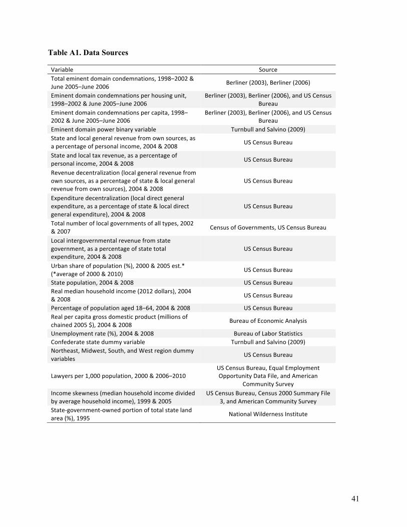
41

Table A1. Data Sources

Variable   Source  Total  eminent  domain  condemnations,  1998–2002  &  June  2005–June  2006  

Berliner  (2003),  Berliner  (2006)  

Eminent  domain  condemnations  per  housing  unit,  1998–2002  &  June  2005–June  2006  

Berliner  (2003),  Berliner  (2006),  and  US  Census  Bureau  

Eminent  domain  condemnations  per  capita,  1998–2002  &  June  2005–June  2006  

Berliner  (2003),  Berliner  (2006),  and  US  Census  Bureau  

Eminent  domain  power  binary  variable   Turnbull  and  Salvino  (2009)  State  and  local  general  revenue  from  own  sources,  as  a  percentage  of  personal  income,  2004  &  2008   US  Census  Bureau  

State  and  local  tax  revenue,  as  a  percentage  of  personal  income,  2004  &  2008   US  Census  Bureau  

Revenue  decentralization  (local  general  revenue  from  own  sources,  as  a  percentage  of  state  &  local  general  revenue  from  own  sources),  2004  &  2008  

US  Census  Bureau  

Expenditure  decentralization  (local  direct  general  expenditure,  as  a  percentage  of  state  &  local  direct  general  expenditure),  2004  &  2008  

US  Census  Bureau  

Total  number  of  local  governments  of  all  types,  2002  &  2007   Census  of  Governments,  US  Census  Bureau  

Local  intergovernmental  revenue  from  state  government,  as  a  percentage  of  state  total  expenditure,  2004  &  2008  

US  Census  Bureau  

Urban  share  of  population  (%),  2000  &  2005  est.*  (*average  of  2000  &  2010)  

US  Census  Bureau  

State  population,  2004  &  2008   US  Census  Bureau  Real  median  household  income  (2012  dollars),  2004  &  2008   US  Census  Bureau  

Percentage  of  population  aged  18–64,  2004  &  2008   US  Census  Bureau  Real  per  capita  gross  domestic  product  (millions  of  chained  2005  $),  2004  &  2008  

Bureau  of  Economic  Analysis  

Unemployment  rate  (%),  2004  &  2008   Bureau  of  Labor  Statistics  Confederate  state  dummy  variable   Turnbull  and  Salvino  (2009)  Northeast,  Midwest,  South,  and  West  region  dummy  variables   US  Census  Bureau  

Lawyers  per  1,000  population,  2000  &  2006–2010  US  Census  Bureau,  Equal  Employment  Opportunity  Data  File,  and  American  

Community  Survey  Income  skewness  (median  household  income  divided  by  average  household  income),  1999  &  2005  

US  Census  Bureau,  Census  2000  Summary  File  3,  and  American  Community  Survey  

State-­‐government-­‐owned  portion  of  total  state  land  area  (%),  1995  

National  Wilderness  Institute  

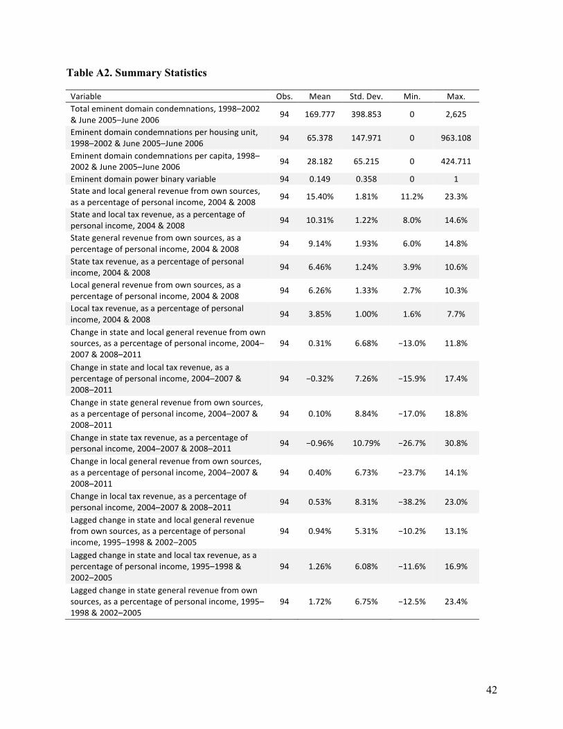
42

Table A2. Summary Statistics

Variable   Obs.   Mean   Std.  Dev.   Min.   Max.  Total  eminent  domain  condemnations,  1998–2002  &  June  2005–June  2006  

94   169.777   398.853   0   2,625  

Eminent  domain  condemnations  per  housing  unit,  1998–2002  &  June  2005–June  2006   94   65.378   147.971   0   963.108  

Eminent  domain  condemnations  per  capita,  1998–2002  &  June  2005–June  2006   94   28.182   65.215   0   424.711  

Eminent  domain  power  binary  variable   94   0.149   0.358   0   1  State  and  local  general  revenue  from  own  sources,  as  a  percentage  of  personal  income,  2004  &  2008  

94   15.40%   1.81%   11.2%   23.3%  

State  and  local  tax  revenue,  as  a  percentage  of  personal  income,  2004  &  2008   94   10.31%   1.22%   8.0%   14.6%  

State  general  revenue  from  own  sources,  as  a  percentage  of  personal  income,  2004  &  2008   94   9.14%   1.93%   6.0%   14.8%  

State  tax  revenue,  as  a  percentage  of  personal  income,  2004  &  2008  

94   6.46%   1.24%   3.9%   10.6%  

Local  general  revenue  from  own  sources,  as  a  percentage  of  personal  income,  2004  &  2008  

94   6.26%   1.33%   2.7%   10.3%  

Local  tax  revenue,  as  a  percentage  of  personal  income,  2004  &  2008   94   3.85%   1.00%   1.6%   7.7%  

Change  in  state  and  local  general  revenue  from  own  sources,  as  a  percentage  of  personal  income,  2004–2007  &  2008–2011  

94   0.31%   6.68%   −13.0%   11.8%  

Change  in  state  and  local  tax  revenue,  as  a  percentage  of  personal  income,  2004–2007  &  2008–2011  

94   −0.32%   7.26%   −15.9%   17.4%  

Change  in  state  general  revenue  from  own  sources,  as  a  percentage  of  personal  income,  2004–2007  &  2008–2011  

94   0.10%   8.84%   −17.0%   18.8%  

Change  in  state  tax  revenue,  as  a  percentage  of  personal  income,  2004–2007  &  2008–2011   94   −0.96%   10.79%   −26.7%   30.8%  

Change  in  local  general  revenue  from  own  sources,  as  a  percentage  of  personal  income,  2004–2007  &  2008–2011  

94   0.40%   6.73%   −23.7%   14.1%  

Change  in  local  tax  revenue,  as  a  percentage  of  personal  income,  2004–2007  &  2008–2011   94   0.53%   8.31%   −38.2%   23.0%  

Lagged  change  in  state  and  local  general  revenue  from  own  sources,  as  a  percentage  of  personal  income,  1995–1998  &  2002–2005  

94   0.94%   5.31%   −10.2%   13.1%  

Lagged  change  in  state  and  local  tax  revenue,  as  a  percentage  of  personal  income,  1995–1998  &  2002–2005  

94   1.26%   6.08%   −11.6%   16.9%  

Lagged  change  in  state  general  revenue  from  own  sources,  as  a  percentage  of  personal  income,  1995–1998  &  2002–2005  

94   1.72%   6.75%   −12.5%   23.4%  

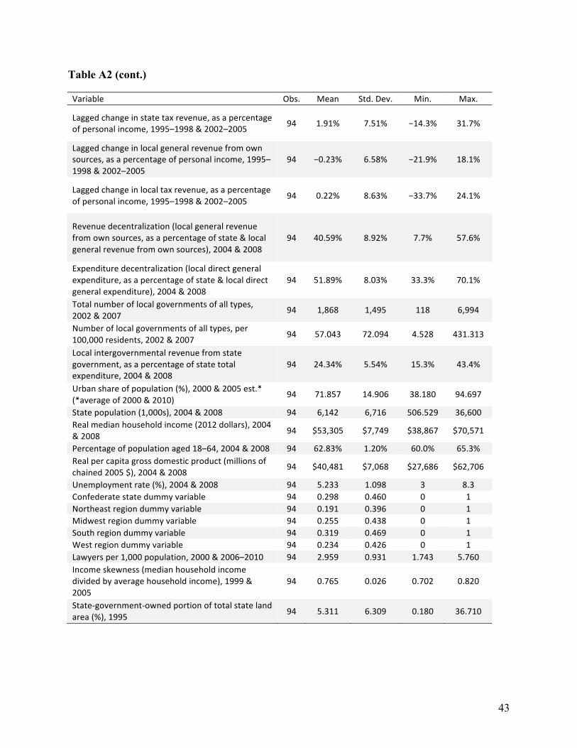
43

Table A2 (cont.)

Variable   Obs.   Mean   Std.  Dev.   Min.   Max.  

Lagged  change  in  state  tax  revenue,  as  a  percentage  of  personal  income,  1995–1998  &  2002–2005   94   1.91%   7.51%   −14.3%   31.7%  

Lagged  change  in  local  general  revenue  from  own  sources,  as  a  percentage  of  personal  income,  1995–1998  &  2002–2005  

94   −0.23%   6.58%   −21.9%   18.1%  

Lagged  change  in  local  tax  revenue,  as  a  percentage  of  personal  income,  1995–1998  &  2002–2005   94   0.22%   8.63%   −33.7%   24.1%  

Revenue  decentralization  (local  general  revenue  from  own  sources,  as  a  percentage  of  state  &  local  general  revenue  from  own  sources),  2004  &  2008  

94   40.59%   8.92%   7.7%   57.6%  

Expenditure  decentralization  (local  direct  general  expenditure,  as  a  percentage  of  state  &  local  direct  general  expenditure),  2004  &  2008  

94   51.89%   8.03%   33.3%   70.1%  

Total  number  of  local  governments  of  all  types,  2002  &  2007  

94   1,868   1,495   118   6,994  

Number  of  local  governments  of  all  types,  per  100,000  residents,  2002  &  2007   94   57.043   72.094   4.528   431.313  

Local  intergovernmental  revenue  from  state  government,  as  a  percentage  of  state  total  expenditure,  2004  &  2008  

94   24.34%   5.54%   15.3%   43.4%  

Urban  share  of  population  (%),  2000  &  2005  est.*  (*average  of  2000  &  2010)  

94   71.857   14.906   38.180   94.697  

State  population  (1,000s),  2004  &  2008   94   6,142   6,716   506.529   36,600  Real  median  household  income  (2012  dollars),  2004  &  2008   94   $53,305   $7,749   $38,867   $70,571  

Percentage  of  population  aged  18–64,  2004  &  2008   94   62.83%   1.20%   60.0%   65.3%  Real  per  capita  gross  domestic  product  (millions  of  chained  2005  $),  2004  &  2008  

94   $40,481   $7,068   $27,686   $62,706  

Unemployment  rate  (%),  2004  &  2008   94   5.233   1.098   3   8.3  Confederate  state  dummy  variable   94   0.298   0.460   0   1  Northeast  region  dummy  variable   94   0.191   0.396   0   1  Midwest  region  dummy  variable   94   0.255   0.438   0   1  South  region  dummy  variable   94   0.319   0.469   0   1  West  region  dummy  variable   94   0.234   0.426   0   1  Lawyers  per  1,000  population,  2000  &  2006–2010   94   2.959   0.931   1.743   5.760  Income  skewness  (median  household  income  divided  by  average  household  income),  1999  &  2005  

94   0.765   0.026   0.702   0.820  

State-­‐government-­‐owned  portion  of  total  state  land  area  (%),  1995   94   5.311   6.309   0.180   36.710  

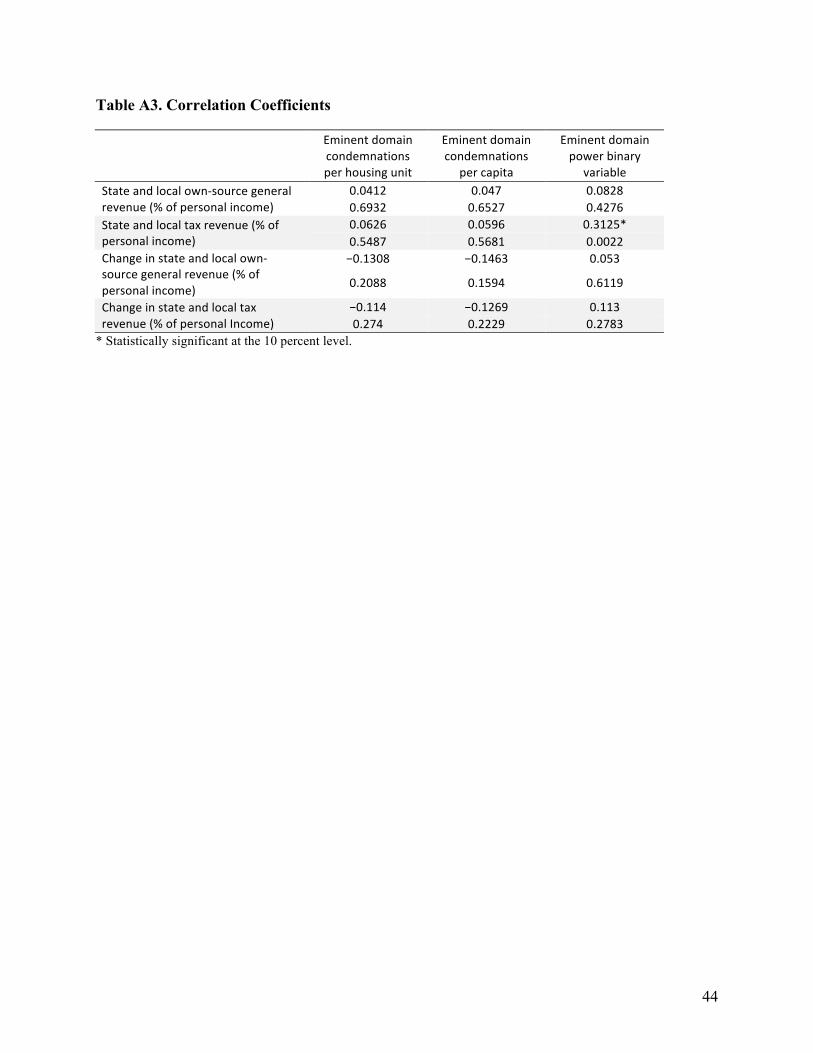
44

Table A3. Correlation Coefficients

 

Eminent  domain  condemnations  per  housing  unit  

Eminent  domain  condemnations  

per  capita  

Eminent  domain  power  binary  

variable  State  and  local  own-­‐source  general  revenue  (%  of  personal  income)  

0.0412   0.047   0.0828  0.6932   0.6527   0.4276  

State  and  local  tax  revenue  (%  of  personal  income)  

0.0626   0.0596   0.3125*  0.5487   0.5681   0.0022  

Change  in  state  and  local  own-­‐source  general  revenue  (%  of  personal  income)  

−0.1308   −0.1463   0.053  

0.2088   0.1594   0.6119  

Change  in  state  and  local  tax  revenue  (%  of  personal  Income)  

−0.114   −0.1269   0.113  0.274   0.2229   0.2783  

* Statistically significant at the 10 percent level.

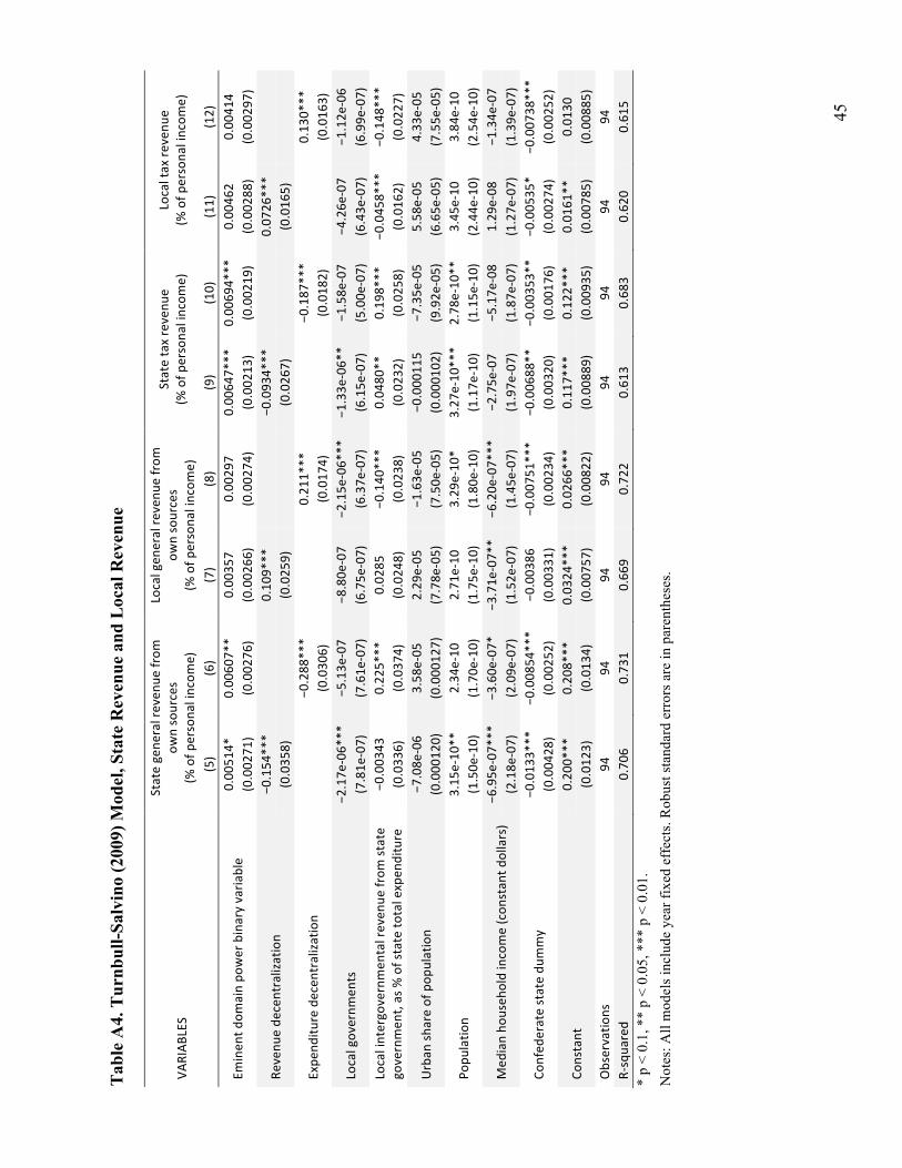
45

Tab

le A

4. T

urnb

ull-S

alvi

no (2

009)

Mod

el, S

tate

Rev

enue

and

Loc

al R

even

ue

VARIAB

LES  

State  gene

ral  reven

ue  from

 ow

n  sources  

(%  of  p

ersona

l  incom

e)  

Local  gen

eral  re

venu

e  from

 ow

n  sources  

(%  of  p

ersona

l  incom

e)  

State  tax  revenu

e  (%

 of  p

ersona

l  incom

e)  

Local  tax  re

venu

e  (%

 of  p

ersona

l  incom

e)  

(5)  

(6)  

(7)  

(8)  

(9)  

(10)  

(11)  

(12)  

Eminen

t  dom

ain  po

wer  binary  varia

ble  

0.00

514*

 0.00

607*

*  0.00

357  

0.00

297  

0.00

647*

**  

0.00

694*

**  

0.00

462  

0.00

414  

(0.002

71)  

(0.002

76)  

(0.002

66)  

(0.002

74)  

(0.002

13)  

(0.002

19)  

(0.002

88)  

(0.002

97)  

Revenu

e  de

centralization  

−0.154

***  

 0.10

9***  

 −0

.093

4***  

 0.07

26***  

 (0.035

8)  

 (0.025

9)  

 (0.026

7)  

 (0.016

5)  

 Expe

nditu

re  decen

tralization  

 −0

.288

***  

 0.21

1***  

 −0

.187

***  

 0.13

0***  

 (0.030

6)  

 (0.017

4)  

 (0.018

2)  

 (0.016

3)  

Local  governm

ents  

−2.17e

-­‐06*

**  

−5.13e

-­‐07  

−8.80e

-­‐07  

−2.15e

-­‐06*

**  

−1.33e

-­‐06*

*  −1

.58e

-­‐07  

−4.26e

-­‐07  

−1.12e

-­‐06  

(7.81e

-­‐07)  

(7.61e

-­‐07)  

(6.75e

-­‐07)  

(6.37e

-­‐07)  

(6.15e

-­‐07)  

(5.00e

-­‐07)  

(6.43e

-­‐07)  

(6.99e

-­‐07)  

Local  intergovernmen

tal  reven

ue  from

 state  

governmen

t,  as  %  of  state  to

tal  expen

diture  

−0.003

43  

0.22

5***  

0.02

85  

−0.140

***  

0.04

80**  

0.19

8***  

−0.045

8***  

−0.148

***  

(0.033

6)  

(0.037

4)  

(0.024

8)  

(0.023

8)  

(0.023

2)  

(0.025

8)  

(0.016

2)  

(0.022

7)  

Urban

 share  of  pop

ulation  

−7.08e

-­‐06  

3.58

e-­‐05

 2.29

e-­‐05

 −1

.63e

-­‐05  

−0.000

115  

−7.35e

-­‐05  

5.58

e-­‐05

 4.33

e-­‐05

 (0.000

120)  

(0.000

127)  

(7.78e

-­‐05)  

(7.50e

-­‐05)  

(0.000

102)  

(9.92e

-­‐05)  

(6.65e

-­‐05)  

(7.55e

-­‐05)  

Popu

latio

n  3.15

e-­‐10

**  

2.34

e-­‐10

 2.71

e-­‐10

 3.29

e-­‐10

*  3.27

e-­‐10

***  

2.78

e-­‐10

**  

3.45

e-­‐10

 3.84

e-­‐10

 (1.50e

-­‐10)  

(1.70e

-­‐10)  

(1.75e

-­‐10)  

(1.80e

-­‐10)  

(1.17e

-­‐10)  

(1.15e

-­‐10)  

(2.44e

-­‐10)  

(2.54e

-­‐10)  

Med

ian  ho

useh

old  income  (con

stan

t  dollars)  

−6.95e

-­‐07*

**  

−3.60e

-­‐07*

 −3

.71e

-­‐07*

*  −6

.20e

-­‐07*

**  

−2.75e

-­‐07  

−5.17e

-­‐08  

1.29

e-­‐08

 −1

.34e

-­‐07  

(2.18e

-­‐07)  

(2.09e

-­‐07)  

(1.52e

-­‐07)  

(1.45e

-­‐07)  

(1.97e

-­‐07)  

(1.87e

-­‐07)  

(1.27e

-­‐07)  

(1.39e

-­‐07)  

Confed

erate  state  du

mmy  

−0.013

3***  

−0.008

54***  

−0.003

86  

−0.007

51***  

−0.006

88**  

−0.003

53**  

−0.005

35*  

−0.007

38***  

(0.004

28)  

(0.002

52)  

(0.003

31)  

(0.002

34)  

(0.003

20)  

(0.001

76)  

(0.002

74)  

(0.002

52)  

Constant  

0.20

0***  

0.20

8***  

0.03

24***  

0.02

66***  

0.11

7***  

0.12

2***  

0.01

61**  

0.01

30  

(0.012

3)  

(0.013

4)  

(0.007

57)  

(0.008

22)  

(0.008

89)  

(0.009

35)  

(0.007

85)  

(0.008

85)  

Observatio

ns  

94  

94  

94  

94  

94  

94  

94  

94  

R-­‐squa

red  

0.70

6  0.73

1  0.66

9  0.72

2  0.61

3  0.68

3  0.62

0  0.61

5  *

p <

0.1,

**

p <

0.05

, ***

p <

0.0

1.

Not

es: A

ll m

odel

s inc

lude

yea

r fix

ed e

ffec

ts. R

obus

t sta

ndar

d er

rors

are

in p

aren

thes

es.

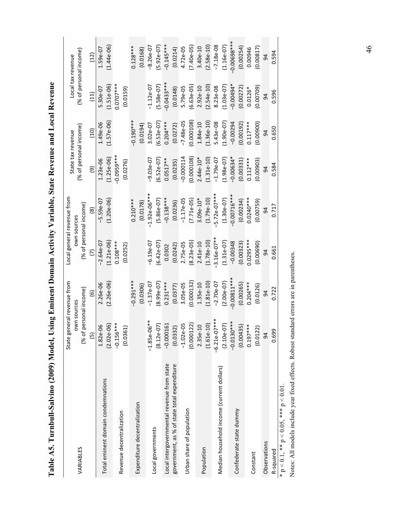
46

Tab

le A

5. T

urnb

ull-S

alvi

no (2

009)

Mod

el, U

sing

Em

inen

t Dom

ain

Act

ivity

Var

iabl

e, S

tate

Rev

enue

and

Loc

al R

even

ue

VARIAB

LES  

State  gene

ral  reven

ue  from

 ow

n  sources  

(%  of  p

ersona

l  incom

e)  

Local  gen

eral  re

venu

e  from

 ow

n  sources  

(%  of  p

ersona

l  incom

e)  

State  tax  revenu

e  (%

 of  p

ersona

l  incom

e)  

Local  tax  re

venu

e  (%

 of  p

ersona

l  incom

e)  

(5)  

(6)  

(7)  

(8)  

(9)  

(10)  

(11)  

(12)  

Total  eminen

t  dom

ain  cond

emna

tions  

1.82

e-­‐06

 2.26

e-­‐06

 −2

.64e

-­‐07  

−5.59e

-­‐07  

1.23

e-­‐06

 1.49

e-­‐06

 5.30

e-­‐07

 1.59

e-­‐07

 (2.02e

-­‐06)  

(2.26e

-­‐06)  

(1.21e

-­‐06)  

(1.20e

-­‐06)  

(1.25e

-­‐06)  

(1.57e

-­‐06)  

(1.51e

-­‐06)  

(1.44e

-­‐06)  

Revenu

e  de

centralization  

−0.156

***  

 0.10

8***  

 −0

.095

9***  

 0.07

07***  

 (0.036

1)  

 (0.025

2)  

 (0.027

6)  

 (0.015

9)  

 Expe

nditu

re  decen

tralization  

 −0

.291

***  

 0.21

0***  

 −0

.190

***  

 0.12

8***  

 (0.030

6)  

 (0.017

8)  

 (0.019

4)  

 (0.016

8)  

Local  governm

ents  

−1.85e

-­‐06*

*  −1

.37e

-­‐07  

−6.19e

-­‐07  

−1.92e

-­‐06*

**  

−9.03e

-­‐07  

3.02

e-­‐07

 −1

.12e

-­‐07  

−8.26e

-­‐07  

(8.12e

-­‐07)  

(8.99e

-­‐07)  

(6.42e

-­‐07)  

(5.86e

-­‐07)  

(6.52e

-­‐07)  

(6.53e

-­‐07)  

(5.58e

-­‐07)  

(5.92e

-­‐07)  

Local  intergovernmen

tal  reven

ue  from

 state  

governmen

t,  as  %  of  state  to

tal  expen

diture  

−0.000

161  

0.23

1***  

0.03

02  

−0.138

***  

0.05

17**  

0.20

4***  

−0.043

3***  

−0.145

***  

(0.033

2)  

(0.037

7)  

(0.024

2)  

(0.023

6)  

(0.023

5)  

(0.027

2)  

(0.014

8)  

(0.021

4)  

Urban

 share  of  pop

ulation  

−1.02e

-­‐05  

3.05

e-­‐05

 2.75

e-­‐05

 −1

.17e

-­‐05  

−0.000

114  

−7.48e

-­‐05  

5.79

e-­‐05

 4.72

e-­‐05

 (0.000

122)  

(0.000

132)  

(8.23e

-­‐05)  

(7.71e

-­‐05)  

(0.000

108)  

(0.000

108)  

(6.63e

-­‐05)  

(7.40e

-­‐05)  

Popu

latio

n  2.35

e-­‐10

 1.35

e-­‐10

 2.41

e-­‐10

 3.09

e-­‐10

*  2.44

e-­‐10

*  1.84

e-­‐10

 2.92

e-­‐10

 3.40

e-­‐10

 (1.61e

-­‐10)  

(1.81e

-­‐10)  

(1.78e

-­‐10)  

(1.79e

-­‐10)  

(1.31e

-­‐10)  

(1.36e

-­‐10)  

(2.54e

-­‐10)  

(2.58e

-­‐10)  

Med

ian  ho

useh

old  income  (current  dollars)  

−6.21e

-­‐07*

**  

−2.70e

-­‐07  

−3.16e

-­‐07*

*  −5

.72e

-­‐07*

**  

−1.79e

-­‐07  

5.43

e−08

 8.23

e-­‐08

 −7

.18e

-­‐08  

(2.10e

-­‐07)  

(2.00e

-­‐07)  

(1.31e

-­‐07)  

(1.30e

-­‐07)  

(1.98e

-­‐07)  

(1.90e

-­‐07)  

(1.03e

-­‐07)  

(1.16e

-­‐07)  

Confed

erate  state  du

mmy  

−0.013

0***  

−0.008

11***  

−0.003

48  

−0.007

16***  

−0.006

34*  

−0.002

94  

−0.004

94*  

−0.006

98***  

(0.004

35)  

(0.002

65)  

(0.003

23)  

(0.002

34)  

(0.003

31)  

(0.001

92)  

(0.002

72)  

(0.002

54)  

Constant  

0.19

7***  

0.20

4***  

0.02

95***  

0.02

40***  

0.11

2***  

0.11

7***  

0.01

26*  

0.00

946  

(0.012

2)  

(0.012

6)  

(0.006

90)  

(0.007

59)  

(0.009

03)  

(0.009

00)  

(0.007

09)  

(0.008

17)  

Observatio

ns  

94  

94  

94  

94  

94  

94  

94  

94  

R-­‐squa

red  

0.69

9  0.72

2  0.66

1  0.71

7  0.58

4  0.65

0  0.59

6  0.59

4  *

p <

0.1,

**

p <

0.05

, ***

p <

0.0

1.

Not

es: A

ll m

odel

s inc

lude

yea

r fix

ed e

ffec

ts. R

obus

t sta

ndar

d er

rors

are

in p

aren

thes

es.

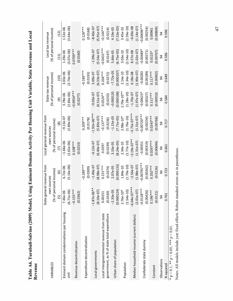
47

Tab

le A

6. T

urnb

ull-S

alvi

no (2

009)

Mod

el, U

sing

Em

inen

t Dom

ain

Act

ivity

Per

Hou

sing

Uni

t Var

iabl

e, S

tate

Rev

enue

and

Loc

al

Rev

enue

VARIAB

LES  

State  gene

ral  reven

ue  from

 ow

n  sources  

(%  of  p

ersona

l  incom

e)  

Local  gen

eral  re

venu

e  from

 ow

n  sources  

(%  of  p

ersona

l  incom

e)  

State  tax  revenu

e  (%

 of  p

ersona

l  incom

e)  

Local  tax  re

venu

e  (%

 of  p

ersona

l  incom

e)  

(5)  

(6)  

(7)  

(8)  

(9)  

(10)  

(11)  

(12)  

Eminen

t  dom

ain  cond

emna

tions  per  hou

sing  

unit  

7.46

e-­‐06

 6.72

e-­‐06

 −1

.66e

-­‐06  

−9.13e

-­‐07  

3.78

e-­‐06

 3.03

e-­‐06

 1.29

e-­‐06

 1.52

e-­‐06

 (6.71e

-­‐06)  

(5.10e

-­‐06)  

(2.65e

-­‐06)  

(2.89e

-­‐06)  

(2.84e

-­‐06)  

(2.74e

-­‐06)  

(3.07e

-­‐06)  

(3.64e

-­‐06)  

Revenu

e  de

centralization  

−0.155

***  

 0.10

8***  

 −0

.095

4***  

 0.07

09***  

 (0.036

2)  

 (0.025

3)  

 (0.027

7)  

 (0.016

0)  

 Expe

nditu

re  decen

tralization  

 −0

.289

***  

 0.20

9***  

 −0

.189

***  

 0.12

8***  

 (0.030

9)  

 (0.017

8)  

 (0.019

3)  

 (0.016

8)  

Local  governm

ents  

−1.87e

-­‐06*

*  −1

.49e

-­‐07  

−6.12e

-­‐07  

−1.92e

-­‐06*

**  

−9.03e

-­‐07  

3.09

e-­‐07

 −1

.09e

-­‐07  

−8.40e

-­‐07  

(8.10e

-­‐07)  

(8.98e

-­‐07)  

(6.40e

-­‐07)  

(5.83e

-­‐07)  

(6.51e

-­‐07)  

(6.53e

-­‐07)  

(5.54e

-­‐07)  

(5.91e

-­‐07)  

Local  intergovernmen

tal  reven

ue  from

 state  

governmen

t,  as  %  of  state  to

tal  expen

diture  

0.00

151  

0.23

1***  

0.02

97  

−0.137

***  

0.05

24**  

0.20

4***  

−0.043

1***  

−0.144

***  

(0.033

0)  

(0.037

4)  

(0.023

9)  

(0.023

6)  

(0.023

3)  

(0.027

2)  

(0.014

7)  

(0.021

4)  

Urban

 share  of  pop

ulation  

−2.33e

-­‐05  

2.07

e-­‐05

 3.10

e-­‐05

 −1

.15e

-­‐05  

−0.000

120  

−7.72e

-­‐05  

5.66

e-­‐05

 4.19

e-­‐05

 (0.000

124)  

(0.000

133)  

(8.24e

-­‐05)  

(7.71e

-­‐05)  

(0.000

108)  

(0.000

107)  

(6.75e

-­‐05)  

(7.53e

-­‐05)  

Popu

latio

n  2.76

e-­‐10

*  1.84

e-­‐10

 2.34

e-­‐10

 2.98

e-­‐10

*  2.70

e-­‐10

**  

2.14

e-­‐10

 3.03

e-­‐10

 3.45

e-­‐10

 (1.54e

-­‐10)  

(1.79e

-­‐10)  

(1.77e

-­‐10)  

(1.76e

-­‐10)  

(1.28e

-­‐10)  

(1.34e

-­‐10)  

(2.54e

-­‐10)  

(2.59e

-­‐10)  

Med

ian  ho

useh

old  income  (current  dollars)  

−6.04e

-­‐07*

**  

−2.56e

-­‐07  

−3.19e

-­‐07*

*  −5

.75e

-­‐07*

**  

−1.70e

-­‐07  

6.18

e-­‐08

 8.57

e-­‐08

 −6

.69e

-­‐08  

(2.01e

-­‐07)  

(1.98e

-­‐07)  

(1.31e

-­‐07)  

(1.31e

-­‐07)  

(1.97e

-­‐07)  

(1.90e

-­‐07)  

(1.02e

-­‐07)  

(1.14e

-­‐07)  

Confed

erate  state  du

mmy  

−0.012

8***  

−0.007

95***  

−0.003

51  

−0.007

20***  

−0.006

23*  

−0.002

83  

−0.004

89*  

−0.006

96***  

(0.004

26)  

(0.002

62)  

(0.003

19)  

(0.002

34)  

(0.003

27)  

(0.001

89)  

(0.002

71)  

(0.002

54)  

Constant  

0.19

6***  

0.20

2***  

0.02

97***  

0.02

43***  

0.11

1***  

0.11

7***  

0.01

23*  

0.00

961  

(0.012

1)  

(0.012

6)  

(0.006

94)  

(0.007

68)  

(0.009

10)  

(0.009

02)  

(0.007

07)  

(0.008

09)  

Observatio

ns  

94  

94  

94  

94  

94  

94  

94  

94  

R-­‐squa

red  

0.70

1  0.72

3  0.66

1  0.71

7  0.58

4  0.64

9  0.59

6  0.59

6  *

p <

0.1,

**

p <

0.05

, ***

p <

0.0

1.

Not

es: A

ll m

odel

s inc

lude

yea

r fix

ed e

ffec

ts. R

obus

t sta

ndar

d er

rors

are

in p

aren

thes

es.

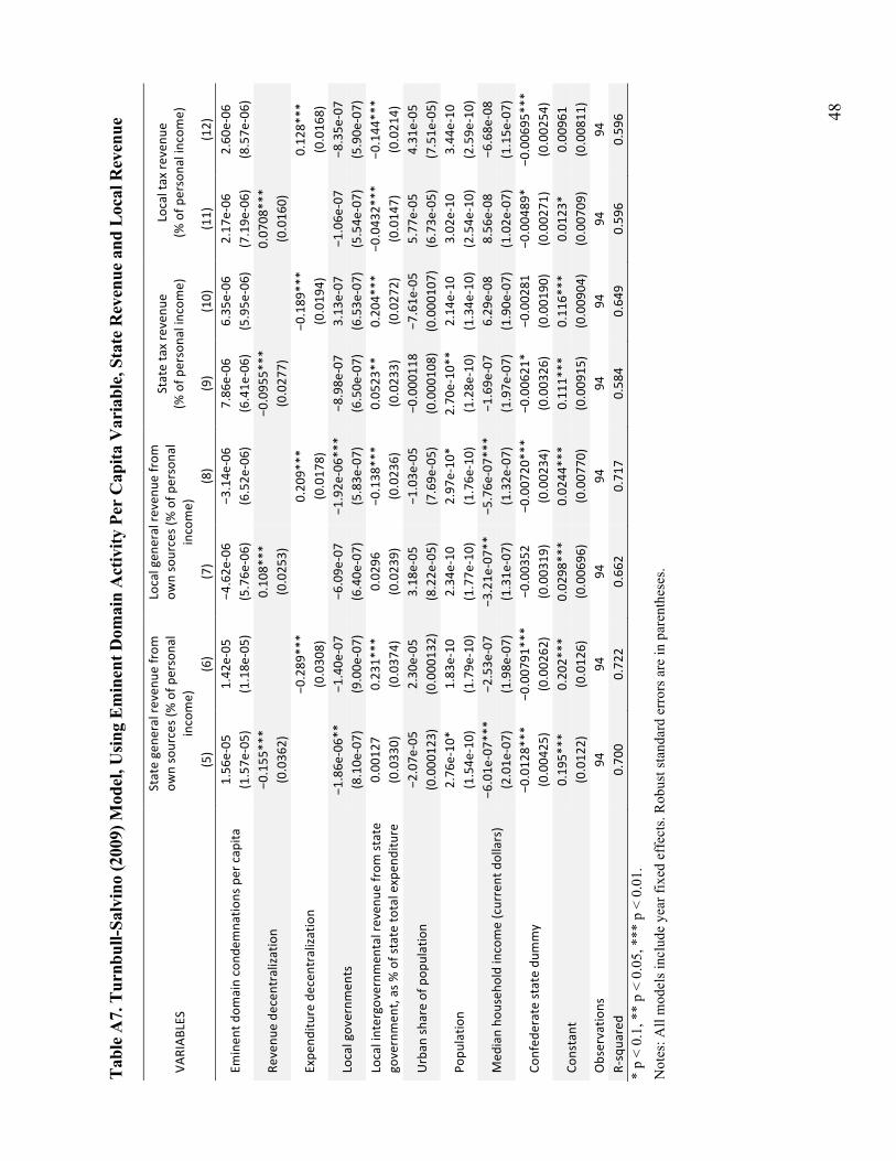
48

Tabl

e A

7. T

urnb

ull-S

alvi

no (2

009)

Mod

el, U

sing

Emin

ent D

omai

n A

ctiv

ity P

er C

apita

Var

iabl

e, S

tate

Rev

enue

and

Loc

al R

even

ue

VARIAB

LES  

State  gene

ral  reven

ue  from

 ow

n  sources  (%  of  p

ersona

l  income)  

Local  gen

eral  re

venu

e  from

 ow

n  sources  (%  of  p

ersona

l  income)  

State  tax  revenu

e  (%

 of  p

ersona

l  incom

e)  

Local  tax  re

venu

e  (%

 of  p

ersona

l  incom

e)  

(5)  

(6)  

(7)  

(8)  

(9)  

(10)  

(11)  

(12)  

Eminen

t  dom

ain  cond

emna

tions  per  cap

ita  

1.56

e-­‐05

 1.42

e-­‐05

 −4

.62e

-­‐06  

−3.14e

-­‐06  

7.86

e-­‐06

 6.35

e-­‐06

 2.17

e-­‐06

 2.60

e-­‐06

 (1.57e

-­‐05)  

(1.18e

-­‐05)  

(5.76e

-­‐06)  

(6.52e

-­‐06)  

(6.41e

-­‐06)  

(5.95e

-­‐06)  

(7.19e

-­‐06)  

(8.57e

-­‐06)  

Revenu

e  de

centralization  

−0.155

***  

 0.10

8***  

 −0

.095

5***  

 0.07

08***  

 (0.036

2)  

 (0.025

3)  

 (0.027

7)  

 (0.016

0)  

 Expe

nditu

re  decen

tralization  

 −0

.289

***  

 0.20

9***  

 −0

.189

***  

 0.12

8***  

 (0.030

8)  

 (0.017

8)  

 (0.019

4)  

 (0.016

8)  

Local  governm

ents  

−1.86e

-­‐06*

*  −1

.40e

-­‐07  

−6.09e

-­‐07  

−1.92e

-­‐06*

**  

−8.98e

-­‐07  

3.13

e-­‐07

 −1

.06e

-­‐07  

−8.35e

-­‐07  

(8.10e

-­‐07)  

(9.00e

-­‐07)  

(6.40e

-­‐07)  

(5.83e

-­‐07)  

(6.50e

-­‐07)  

(6.53e

-­‐07)  

(5.54e

-­‐07)  

(5.90e

-­‐07)  

Local  intergovernmen

tal  reven

ue  from

 state  

governmen

t,  as  %  of  state  to

tal  expen

diture  

0.00

127  

0.23

1***  

0.02

96  

−0.138

***  

0.05

23**  

0.20

4***  

−0.043

2***  

−0.144

***  

(0.033

0)  

(0.037

4)  

(0.023

9)  

(0.023

6)  

(0.023

3)  

(0.027

2)  

(0.014

7)  

(0.021

4)  

Urban

 share  of  pop

ulation  

−2.07e

-­‐05  

2.30

e-­‐05

 3.18

e-­‐05

 −1

.03e

-­‐05  

−0.000

118  

−7.61e

-­‐05  

5.77

e-­‐05

 4.31

e-­‐05

 (0.000

123)  

(0.000

132)  

(8.22e

-­‐05)  

(7.69e

-­‐05)  

(0.000

108)  

(0.000

107)  

(6.73e

-­‐05)  

(7.51e

-­‐05)  

Popu

latio

n  2.76

e-­‐10

*  1.83

e-­‐10

 2.34

e-­‐10

 2.97

e-­‐10

*  2.70

e-­‐10

**  

2.14

e-­‐10

 3.02

e-­‐10

 3.44

e-­‐10

 (1.54e

-­‐10)  

(1.79e

-­‐10)  

(1.77e

-­‐10)  

(1.76e

-­‐10)  

(1.28e

-­‐10)  

(1.34e

-­‐10)  

(2.54e

-­‐10)  

(2.59e

-­‐10)  

Med

ian  ho

useh

old  income  (current  dollars)  

−6.01e

-­‐07*

**  

−2.53e

-­‐07  

−3.21e

-­‐07*

*  −5

.76e

-­‐07*

**  

−1.69e

-­‐07  

6.29

e-­‐08

 8.56

e-­‐08

 −6

.68e

-­‐08  

(2.01e

-­‐07)  

(1.98e

-­‐07)  

(1.31e

-­‐07)  

(1.32e

-­‐07)  

(1.97e

-­‐07)  

(1.90e

-­‐07)  

(1.02e

-­‐07)  

(1.15e

-­‐07)  

Confed

erate  state  du

mmy  

−0.012

8***  

−0.007

91***  

−0.003

52  

−0.007

20***  

−0.006

21*  

−0.002

81  

−0.004

89*  

−0.006

95***  

(0.004

25)  

(0.002

62)  

(0.003

19)  

(0.002

34)  

(0.003

26)  

(0.001

90)  

(0.002

71)  

(0.002

54)  

Constant  

0.19

5***  

0.20

2***  

0.02

98***  

0.02

44***  

0.11

1***  

0.11

6***  

0.01

23*  

0.00

961  

(0.012

2)  

(0.012

6)  

(0.006

96)  

(0.007

70)  

(0.009

15)  

(0.009

04)  

(0.007

09)  

(0.008

11)  

Observatio

ns  

94  

94  

94  

94  

94  

94  

94  

94  

R-­‐squa

red  

0.70

0  0.72

2  0.66

2  0.71

7  0.58

4  0.64

9  0.59

6  0.59

6  *

p <

0.1,

**

p <

0.05

, ***

p <

0.0

1.

Not

es: A

ll m

odel

s inc

lude

yea

r fix

ed e

ffec

ts. R

obus

t sta

ndar

d er

rors

are

in p

aren

thes

es.

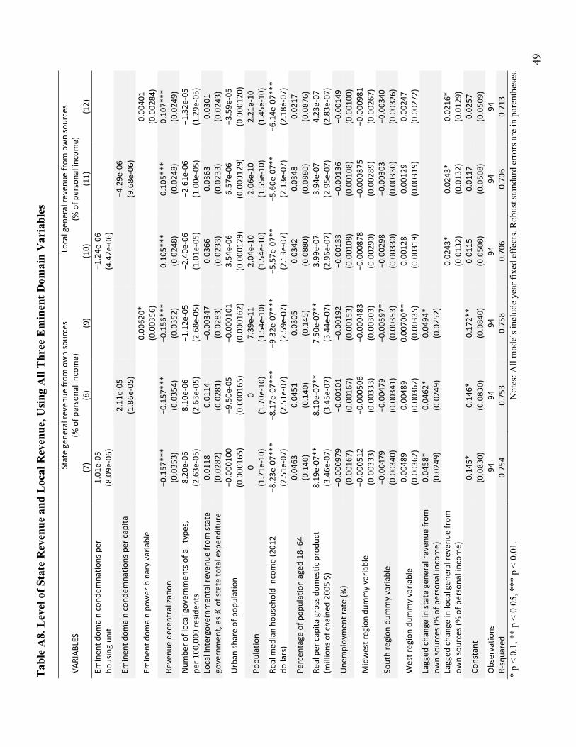
49

Tab

le A

8. L

evel

of S

tate

Rev

enue

and

Loc

al R

even

ue, U

sing

All

Thr

ee E

min

ent D

omai

n V

aria

bles

VARIAB

LES  

State  gene

ral  reven

ue  from

 own  sources  

(%  of  p

ersona

l  incom

e)  

Local  gen

eral  re

venu

e  from

 own  sources  

(%  of  p

ersona

l  incom

e)  

(7)  

(8)  

(9)  

(10)  

(11)  

(12)  

Eminen

t  dom

ain  cond

emna

tions  per    

housing  un

it  1.01

e-­‐05

   

 −1

.24e

-­‐06  

   

(8.09e

-­‐06)  

   

(4.42e

-­‐06)  

   

Eminen

t  dom

ain  cond

emna

tions  per  cap

ita  

 2.11

e-­‐05

   

 −4

.29e

-­‐06  

   

(1.86e

-­‐05)  

   

(9.68e

-­‐06)  

 Em

inen

t  dom

ain  po

wer  binary  varia

ble  

   

0.00

620*

   

 0.00

401  

   

(0.003

56)  

   

(0.002

84)  

Revenu

e  de

centralization  

−0.157

***  

−0.157

***  

−0.156

***  

0.10

5***  

0.10

5***  

0.10

7***  

(0.035

3)  

(0.035

4)  

(0.035

2)  

(0.024

8)  

(0.024

8)  

(0.024

9)  

Num

ber  o

f  local  governm

ents  of  a

ll  type

s,  

per  1

00,000

 resid

ents  

8.20

e-­‐06

 8.10

e-­‐06

 −1

.12e

-­‐05  

−2.40e

-­‐06  

−2.61e

-­‐06  

−1.32e

-­‐05  

(2.63e

-­‐05)  

(2.63e

-­‐05)  

(2.68e

-­‐05)  

(1.01e

-­‐05)  

(1.00e

-­‐05)  

(1.29e

-­‐05)  

Local  intergovernmen

tal  reven

ue  from

 state  

governmen

t,  as  %  of  state  to

tal  expen

diture  

0.01

18  

0.01

14  

−0.003

47  

0.03

66  

0.03

63  

0.03

01  

(0.028

2)  

(0.028

1)  

(0.028

3)  

(0.023

3)  

(0.023

3)  

(0.024

3)  

Urban

 share  of  pop

ulation  

−0.000

100  

−9.50e

-­‐05  

−0.000

101  

3.54

e-­‐06

 6.57

e-­‐06

 −3

.59e

-­‐05  

(0.000

165)  

(0.000

165)  

(0.000

162)  

(0.000

129)  

(0.000

129)  

(0.000

120)  

Popu

latio

n  0  

0  7.39

e-­‐11

 2.04

e-­‐10

 2.06

e-­‐10

 2.21

e-­‐10

 (1.71e

-­‐10)  

(1.70e

-­‐10)  

(1.54e

-­‐10)  

(1.54e

-­‐10)  

(1.55e

-­‐10)  

(1.45e

-­‐10)  

Real  m

edian  ho

useh

old  income  (201

2  do

llars)  

−8.23e

-­‐07*

**  

−8.17e

-­‐07*

**  

−9.32e

-­‐07*

**  

−5.57e

-­‐07*

*  −5

.60e

-­‐07*

*  −6

.14e

-­‐07*

**  

(2.51e

-­‐07)  

(2.51e

-­‐07)  

(2.59e

-­‐07)  

(2.13e

-­‐07)  

(2.13e

-­‐07)  

(2.18e

-­‐07)  

Percen

tage  of  p

opulation  aged

 18–

64  

0.04

63  

0.04

51  

0.03

05  

0.03

42  

0.03

48  

0.02

17  

(0.140

)  (0.140

)  (0.145

)  (0.088

0)  

(0.088

0)  

(0.087

6)  

Real  per  cap

ita  gross  dom

estic  produ

ct  

(millions  of  cha

ined

 200

5  $)  

8.19

e-­‐07

**  

8.10

e-­‐07

**  

7.50

e-­‐07

**  

3.99

e-­‐07

 3.94

e-­‐07

 4.23

e-­‐07

 (3.46e

-­‐07)  

(3.45e

-­‐07)  

(3.44e

-­‐07)  

(2.96e

-­‐07)  

(2.95e

-­‐07)  

(2.83e

-­‐07)  

Une

mploymen

t  rate  (%

)  −0

.000

979  

−0.001

01  

−0.001

92  

−0.001

33  

−0.001

36  

−0.001

49  

(0.001

67)  

(0.001

67)  

(0.001

53)  

(0.001

08)  

(0.001

08)  

(0.001

00)  

Midwest  region  du

mmy  varia

ble  

−0.000

512  

−0.000

506  

−0.000

483  

−0.000

878  

−0.000

875  

−0.000

981  

(0.003

33)  

(0.003

33)  

(0.003

03)  

(0.002

90)  

(0.002

89)  

(0.002

67)  

South  region

 dum

my  varia

ble  

−0.004

79  

−0.004

79  

−0.005

97*  

−0.002

98  

−0.003

03  

−0.003

40  

(0.003

40)  

(0.003

41)  

(0.003

53)  

(0.003

30)  

(0.003

30)  

(0.003

26)  

West  region  du

mmy  varia

ble  

0.00

489  

0.00

489  

0.00

700*

*  0.00

128  

0.00

129  

0.00

247  

(0.003

62)  

(0.003

62)  

(0.003

35)  

(0.003

19)  

(0.003

19)  

(0.002

72)  

Lagged

 cha

nge  in  state  gene

ral  reven

ue  from

 ow

n  sources  (%  of  p

ersona

l  incom

e)  

0.04

58*  

0.04

62*  

0.04

94*  

   

 (0.024

9)  

(0.024

9)  

(0.025

2)  

   

 Lagged

 cha

nge  in  local  gen

eral  re

venu

e  from

 ow

n  sources  (%  of  p

ersona

l  incom

e)  

   

 0.02

43*  

0.02

43*  

0.02

16*  

   

 (0.013

2)  

(0.013

2)  

(0.012

9)  

Constant  

0.14

5*  

0.14

6*  

0.17

2**  

0.01

15  

0.01

17  

0.02

57  

(0.083

0)  

(0.083

0)  

(0.084

0)  

(0.050

8)  

(0.050

8)  

(0.050

9)  

Observatio

ns  

94  

94  

94  

94  

94  

94  

R-­‐squa

red  

0.75

4  0.75

3  0.75

8  0.70

6  0.70

6  0.71

3  *

p <

0.1,

**

p <

0.05

, ***

p <

0.0

1.

Not

es: A

ll m

odel

s inc

lude

yea

r fix

ed e

ffec

ts. R

obus

t sta

ndar

d er

rors

are

in p

aren

thes

es.

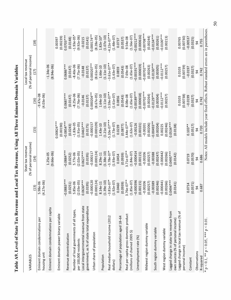
50

Tab

le A

9. L

evel

of S

tate

Tax

Rev

enue

and

Loc

al T

ax R

even

ue, U

sing

All

Thr

ee E

min

ent D

omai

n V

aria

bles

VARIAB

LES  

State  tax  revenu

e  (%

 of  p

ersona

l  incom

e)  

Local  tax  re

venu

e  (%

 of  p

ersona

l  incom

e)  

(13)  

(14)  

(15)  

(16)  

(17)  

(18)  

Eminen

t  dom

ain  cond

emna

tions  per    

housing  un

it  5.98

e-­‐06

   

 −9

.47e

-­‐08  

   

(4.27e

-­‐06)  

   

(4.03e

-­‐06)  

   

Eminen

t  dom

ain  cond

emna

tions  per  cap

ita  

 1.25

e-­‐05

   

 −1

.34e

-­‐06  

   

(9.66e

-­‐06)  

   

(8.94e

-­‐06)  

 Em

inen

t  dom

ain  po

wer  binary  varia

ble  

   

0.00

824*

**  

   

0.00

397  

   

(0.001

90)  

   

(0.002

39)  

Revenu

e  de

centralization  

−0.088

3***  

−0.088

4***  

−0.085

4***  

0.06

87***  

0.06

86***  

0.07

03***  

(0.025

1)  

(0.025

2)  

(0.024

3)  

(0.014

7)  

(0.014

7)  

(0.014

8)  

Num

ber  o

f  local  governm

ents  of  a

ll  type

s,  

per  1

00,000

 resid

ents  

5.85

e-­‐06

 5.77

e-­‐06

 −1

.83e

-­‐05  

−8.25e

-­‐06  

−8.40e

-­‐06  

−1.93e

-­‐05*

 (2.03e

-­‐05)  

(2.02e

-­‐05)  

(1.91e

-­‐05)  

(7.76e

-­‐06)  

(7.75e

-­‐06)  

(9.92e

-­‐06)  

Local  intergovernmen

tal  reven

ue  from

 state  

governmen

t,  as  %  of  state  to

tal  expen

diture  

0.06

30***  

0.06

27***  

0.04

63***  

−0.014

6  −0

.014

8  −0

.021

5  (0.019

5)  

(0.019

5)  

(0.017

5)  

(0.013

7)  

(0.013

7)  

(0.014

1)  

Urban

 share  of  pop

ulation  

−0.000

120  

−0.000

117  

−0.000

157  

0.00

0204

**  

0.00

0207

**  

0.00

0174

**  

(0.000

124)  

(0.000

124)  

(0.000

109)  

(8.67e

-­‐05)  

(8.61e

-­‐05)  

(8.28e

-­‐05)  

Popu

latio

n  8.14

e-­‐11

 8.29

e-­‐11

 1.43

e-­‐10

 1.64

e-­‐10

 1.66

e-­‐10

 1.82

e-­‐10

*  (1.39e

-­‐10)  

(1.38e

-­‐10)  

(1.21e

-­‐10)  

(1.11e

-­‐10)  

(1.11e

-­‐10)  

(1.07e

-­‐10)  

Real  m

edian  ho

useh

old  income  (201

2  do

llars)  

−3.81e

-­‐07*

 −3

.78e

-­‐07*

 −5

.10e

-­‐07*

**  

−3.59e

-­‐07*

*  −3

.61e

-­‐07*

*  −4

.22e

-­‐07*

**  

(1.92e

-­‐07)  

(1.93e

-­‐07)  

(1.73e

-­‐07)  

(1.61e

-­‐07)  

(1.63e

-­‐07)  

(1.48e

-­‐07)  

Percen

tage  of  p

opulation  aged

 18–

64  

0.04

60  

0.04

54  

0.02

39  

0.08

56  

0.08

59  

0.07

37  

(0.093

9)  

(0.093

9)  

(0.087

7)  

(0.054

3)  

(0.054

3)  

(0.053

7)  

Real  per  cap

ita  gross  dom

estic  produ

ct  

(millions  of  cha

ined

 200

5  $)  

3.76

e-­‐07

**  

3.71

e-­‐07

**  

3.44

e-­‐07

**  

8.08

e-­‐08

 7.69

e-­‐08

 9.54

e-­‐08

 (1.85e

-­‐07)  

(1.84e

-­‐07)  

(1.62e

-­‐07)  

(1.65e

-­‐07)  

(1.65e

-­‐07)  

(1.56e

-­‐07)  

Une

mploymen

t  rate  (%

)  −0

.000

396  

−0.000

414  

−0.001

26  

−0.001

89***  

−0.001

91***  

−0.002

12***  

(0.001

15)  

(0.001

15)  

(0.001

01)  

(0.000

658)  

(0.000

659)  

(0.000

616)  

Midwest  region  du

mmy  varia

ble  

−0.002

06  

−0.002

06  

−0.002

01  

−0.007

02***  

−0.007

02***  

−0.007

08***  

(0.002

57)  

(0.002

57)  

(0.002

06)  

(0.002

64)  

(0.002

63)  

(0.002

44)  

South  region

 dum

my  varia

ble  

−0.003

89  

−0.003

88  

−0.004

93**  

−0.012

9***  

−0.013

0***  

−0.013

4***  

(0.002

46)  

(0.002

47)  

(0.002

04)  

(0.003

04)  

(0.003

05)  

(0.002

61)  

West  region  du

mmy  varia

ble  

−0.000

441  

−0.000

442  

0.00

225  

−0.011

2***  

−0.011

2***  

−0.010

0***  

(0.002

66)  

(0.002

66)  

(0.002

46)  

(0.002

57)  

(0.002

57)  

(0.002

13)  

Lagged

 cha

nge  in  state  tax  revenu

e  from

 ow

n  sources  (%  of  p

ersona

l  incom

e)  

0.04

94***  

0.04

95***  

0.05

34***  

   

 (0.014

1)  

(0.014

2)  

(0.013

8)  

   

 Lagged

 cha

nge  in  local  tax  re

venu

e  (%

 of  

person

al  income)  

   

 0.01

03  

0.01

03  

0.00

765  

   

 (0.007

38)  

(0.007

39)  

(0.007

30)  

Constant  

0.07

14  

0.07

19  

0.10

3**  

−0.019

9  −0

.019

7  −0

.005

37  

(0.057

1)  

(0.057

0)  

(0.051

7)  

(0.032

7)  

(0.032

7)  

(0.032

5)  

Observatio

ns  

94  

94  

94  

94  

94  

94  

R-­‐squa

red  

0.68

7  0.68

6  0.72

0  0.74

2  0.74

2  0.75

5  *

p <

0.1,

**

p <

0.05

, ***

p <

0.0

1.

Not

es: A

ll m

odel

s inc

lude

yea

r fix

ed e

ffec

ts. R

obus

t sta

ndar

d er

rors

are

in p

aren

thes

es.

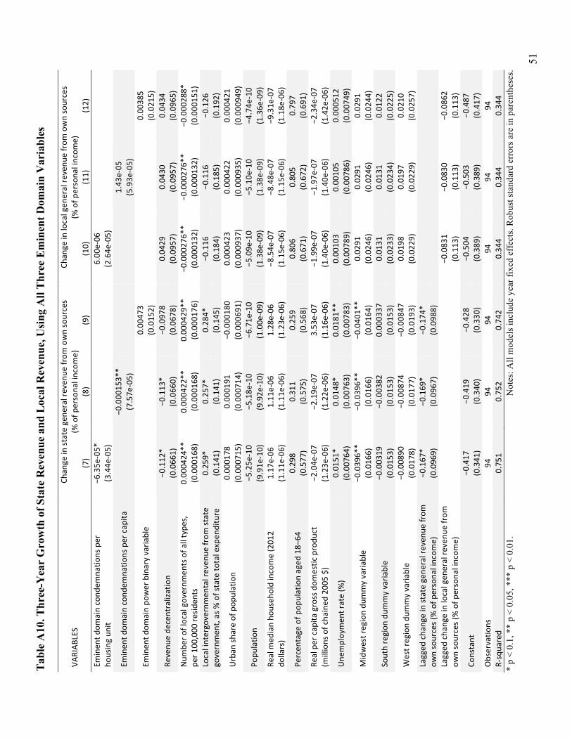
51

Tab

le A

10. T

hree

-Yea

r G

row

th o

f Sta

te R

even

ue a

nd L

ocal

Rev

enue

, Usi

ng A

ll T

hree

Em

inen

t Dom

ain

Var

iabl

es

VARIAB

LES  

Chan

ge  in  state  gene

ral  reven

ue  from

 own  sources  

(%  of  p

ersona

l  incom

e)  

Chan

ge  in  local  gen

eral  re

venu

e  from

 own  sources  

(%  of  p

ersona

l  incom

e)  

(7)  

(8)  

(9)  

(10)  

(11)  

(12)  

Eminen

t  dom

ain  cond

emna

tions  per    

housing  un

it  −6

.35e

-­‐05*

   

 6.00

e-­‐06

   

 (3.44e

-­‐05)  

   

(2.64e

-­‐05)  

   

Eminen

t  dom

ain  cond

emna

tions  per  cap

ita  

 −0

.000

153*

*    

 1.43

e-­‐05

   

 (7.57e

-­‐05)  

   

(5.93e

-­‐05)  

 Em

inen

t  dom

ain  po

wer  binary  varia

ble  

   

0.00

473  

   

0.00

385  

   

(0.015

2)  

   

(0.021

5)  

Revenu

e  de

centralization  

−0.112

*  −0

.113

*  −0

.097

8  0.04

29  

0.04

30  

0.04

34  

(0.066

1)  

(0.066

0)  

(0.067

8)  

(0.095

7)  

(0.095

7)  

(0.096

5)  

Num

ber  o

f  local  governm

ents  of  a

ll  type

s,  

per  1

00,000

 resid

ents  

0.00

0424

**  

0.00

0422

**  

0.00

0429

**  

−0.000

276*

*  −0

.000

276*

*  −0

.000

288*

 (0.000

168)  

(0.000

168)  

(0.000

176)  

(0.000

132)  

(0.000

132)  

(0.000

151)  

Local  intergovernmen

tal  reven

ue  from

 state  

governmen

t,  as  %  of  state  to

tal  expen

diture  

0.25

9*  

0.25

7*  

0.28

4*  

−0.116

 −0

.116

 −0

.126

 (0.141

)  (0.141

)  (0.145

)  (0.184

)  (0.185

)  (0.192

)  

Urban

 share  of  pop

ulation  

0.00

0178

 0.00

0191

 −0

.000

180  

0.00

0423

 0.00

0422

 0.00

0421

 (0.000

715)  

(0.000

714)  

(0.000

691)  

(0.000

937)  

(0.000

935)  

(0.000

949)  

Popu

latio

n  −5

.25e

-­‐10  

−5.18e

-­‐10  

−6.71e

-­‐10  

−5.09e

-­‐10  

−5.10e

-­‐10  

−4.74e

-­‐10  

(9.91e

-­‐10)  

(9.92e

-­‐10)  

(1.00e

-­‐09)  

(1.38e

-­‐09)  

(1.38e

-­‐09)  

(1.36e

-­‐09)  

Real  m

edian  ho

useh

old  income  (201

2  do

llars)  

1.17

e-­‐06

 1.11

e-­‐06

 1.28

e-­‐06

 −8

.54e

-­‐07  

−8.48e

-­‐07  

−9.31e

-­‐07  

(1.11e

-­‐06)  

(1.11e

-­‐06)  

(1.23e

-­‐06)  

(1.15e

-­‐06)  

(1.15e

-­‐06)  

(1.18e

-­‐06)  

Percen

tage  of  p

opulation  aged

 18–

64  

0.29

8  0.31

1  0.25

9  0.80

6  0.80

5  0.79

7  (0.577

)  (0.575

)  (0.568

)  (0.671

)  (0.672

)  (0.691

)  Re

al  per  cap

ita  gross  dom

estic  produ

ct  

(millions  of  cha

ined

 200

5  $)  

−2.04e

-­‐07  

−2.19e

-­‐07  

3.53

e-­‐07

 −1

.99e

-­‐07  

−1.97e

-­‐07  

−2.34e

-­‐07  

(1.23e

-­‐06)  

(1.22e

-­‐06)  

(1.16e

-­‐06)  

(1.40e

-­‐06)  

(1.40e

-­‐06)  

(1.42e

-­‐06)  

Une

mploymen

t  rate  (%

)  0.01

51*  

0.01

48*  

0.01

81**  

0.00

103  

0.00

105  

0.00

0512

 (0.007

64)  

(0.007

63)  

(0.007

83)  

(0.007

89)  

(0.007

86)  

(0.007

49)  

Midwest  region  du

mmy  varia

ble  

−0.039

6**  

−0.039

6**  

−0.040

1**  

0.02

91  

0.02

91  

0.02

91  

(0.016

6)  

(0.016

6)  

(0.016

4)  

(0.024

6)  

(0.024

6)  

(0.024

4)  

South  region

 dum

my  varia

ble  

−0.003

19  

−0.003

82  

0.00

0337

 0.01

31  

0.01

31  

0.01

22  

(0.015

3)  

(0.015

3)  

(0.015

3)  

(0.023

3)  

(0.023

4)  

(0.022

5)  

West  region  du

mmy  varia

ble  

−0.008

90  

−0.008

74  

−0.008

47  

0.01

98  

0.01

97  

0.02

10  

(0.017

8)  

(0.017

7)  

(0.019

3)  

(0.022

9)  

(0.022

9)  

(0.025

7)  

Lagged

 cha

nge  in  state  gene

ral  reven

ue  from

 ow

n  sources  (%  of  p

ersona

l  incom

e)  

−0.167

*  −0

.169

*  −0

.174

*    

   

(0.096

9)  

(0.096

7)  

(0.098

8)  

   

 Lagged

 cha

nge  in  local  gen

eral  re

venu

e  from

 ow

n  sources  (%  of  p

ersona

l  incom

e)  

   

 −0

.083

1  −0

.083

0  −0

.086

2  

   

 (0.113

)  (0.113

)  (0.113

)  

Constant  

−0.417

 −0

.419

 −0

.428

 −0

.504

 −0

.503

 −0

.487

 (0.341

)  (0.340

)  (0.330

)  (0.389

)  (0.389

)  (0.417

)  Observatio

ns  

94  

94  

94  

94  

94  

94  

R-­‐squa

red  

0.75

1  0.75

2  0.74

2  0.34

4  0.34

4  0.34

4  *

p <

0.1,

**

p <

0.05

, ***

p <

0.0

1.

Not

es: A

ll m

odel

s inc

lude

yea

r fix

ed e

ffec

ts. R

obus

t sta

ndar

d er

rors

are

in p

aren

thes

es.

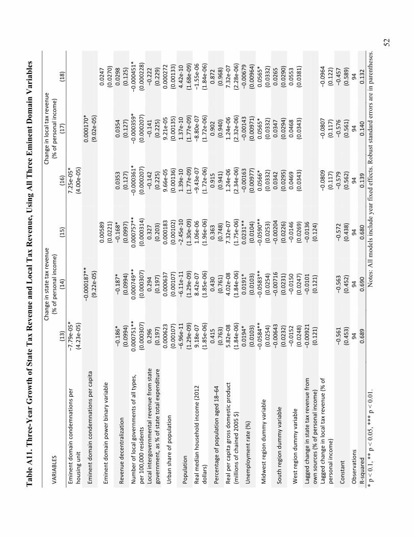
52

Tab

le A

11. T

hree

-Yea

r G

row

th o

f Sta

te T

ax R

even

ue a

nd L

ocal

Tax

Rev

enue

, Usi

ng A

ll T

hree

Em

inen

t Dom

ain

Var

iabl

es

VARIAB

LES  

Chan

ge  in  state  tax  revenu

e  (%

 of  p

ersona

l  incom

e)  

Chan

ge  in  local  tax  re

venu

e  (%

 of  p

ersona

l  incom

e)  

(13)  

(14)  

(15)  

(16)  

(17)  

(18)  

Eminen

t  dom

ain  cond

emna

tions  per    

housing  un

it  −7

.79e

-­‐05*

   

 7.25

e-­‐05

*    

 (4.23e

-­‐05)  

   

(4.00e

-­‐05)  

   

Eminen

t  dom

ain  cond

emna

tions  per  cap

ita  

 −0

.000

187*

*    

 0.00

0170

*    

 (9.22e

-­‐05)  

   

(9.02e

-­‐05)  

 Em

inen

t  dom

ain  po

wer  binary  varia

ble  

   

0.00

589  

   

0.02

47  

   

(0.022

1)  

   

(0.027

0)  

Revenu

e  de

centralization  

−0.186

*  −0

.187

*  −0

.168

*  0.03

53  

0.03

54  

0.02

98  

(0.099

4)  

(0.099

4)  

(0.099

7)  

(0.127

)  (0.127

)  (0.125

)  Num

ber  o

f  local  governm

ents  of  a

ll  type

s,  

per  1

00,000

 resid

ents  

0.00

0751

**  

0.00

0749

**  

0.00

0757

**  

−0.000

361*

 −0

.000

359*

 −0

.000

451*

 (0.000

307)  

(0.000

307)  

(0.000

314)  

(0.000

207)  

(0.000

207)  

(0.000

228)  

Local  intergovernmen

tal  reven

ue  from

 state  

governmen

t,  as  %  of  state  to

tal  expen

diture  

0.29

6  0.29

4  0.32

7  −0

.142

 −0

.141

 −0

.222

 (0.197

)  (0.197

)  (0.203

)  (0.225

)  (0.225

)  (0.229

)  

Urban

 share  of  pop

ulation  

0.00

0623

 0.00

0637

 0.00

0183

 9.66

e-­‐05

 9.21

e-­‐05

 0.00

0272

 (0.001

07)  

(0.001

07)  

(0.001

02)  

(0.001

36)  

(0.001

35)  

(0.001

33)  

Popu

latio

n  −6

.96e

-­‐11  

−6.11e

-­‐11  

−2.45e

-­‐10  

1.39

e-­‐10

 1.37

e-­‐10

 4.42

e-­‐10

 (1.29e

-­‐09)  

(1.29e

-­‐09)  

(1.30e

-­‐09)  

(1.77e

-­‐09)  

(1.77e

-­‐09)  

(1.68e

-­‐09)  

Real  m

edian  ho

useh

old  income  (201

2  do

llars)  

9.18

e-­‐07

 8.42

e-­‐07

 1.06

e-­‐06

 −9

.43e

-­‐07  

−8.80e

-­‐07  

−1.55e

-­‐06  

(1.85e

-­‐06)  

(1.85e

-­‐06)  

(1.96e

-­‐06)  

(1.72e

-­‐06)  

(1.72e

-­‐06)  

(1.84e

-­‐06)  

Percen

tage  of  p

opulation  aged

 18–

64  

0.41

5  0.43

0  0.36

3  0.91

5  0.90

2  0.87

2  (0.763

)  (0.761

)  (0.748

)  (0.941

)  (0.940

)  (0.968

)  Re

al  per  cap

ita  gross  dom

estic  produ

ct  

(millions  of  cha

ined

 200

5  $)  

5.82

e-­‐08

 4.02

e-­‐08

 7.32

e-­‐07

 1.24

e-­‐06

 1.24

e-­‐06

 7.32

e-­‐07

 (1.84e

-­‐06)  

(1.84e

-­‐06)  

(1.75e

-­‐06)  

(2.34e

-­‐06)  

(2.32e

-­‐06)  

(2.28e

-­‐06)  

Une

mploymen

t  rate  (%

)  0.01

94*  

0.01

91*  

0.02

31**  

−0.001

63  

−0.001

43  

−0.006

79  

(0.010

3)  

(0.010

3)  

(0.010

4)  

(0.009

77)  

(0.009

71)  

(0.009

64)  

Midwest  region  du

mmy  varia

ble  

−0.058

4**  

−0.058

3**  

−0.059

0**  

0.05

66*  

0.05

65*  

0.05

65*  

(0.025

4)  

(0.025

4)  

(0.025

3)  

(0.033

2)  

(0.033

2)  

(0.033

2)  

South  region

 dum

my  varia

ble  

−0.006

43  

−0.007

16  

−0.002

04  

0.03

42  

0.03

47  

0.02

65  

(0.023

2)  

(0.023

1)  

(0.022

6)  

(0.029

5)  

(0.029

4)  

(0.029

0)  

West  region  du

mmy  varia

ble  

−0.015

2  −0

.015

0  −0

.014

6  0.04

69  

0.04

68  

0.05

53  

(0.024

8)  

(0.024

7)  

(0.026

9)  

(0.034

3)  

(0.034

3)  

(0.038

1)  

Lagged

 cha

nge  in  state  tax  revenu

e  from

 ow

n  sources  (%  of  p

ersona

l  incom

e)  

−0.009

21  

−0.010

1  −0

.013

6    

   

(0.121

)  (0.121

)  (0.124

)    

   

Lagged

 cha

nge  in  local  tax  re

venu

e  (%

 of  

person

al  income)  

   

 −0

.080

9  −0

.080

7  −0

.096

4  

   

 (0.117

)  (0.117

)  (0.122

)  

Constant  

−0.561

 −0

.563

 −0

.572

 −0

.579

 −0

.576

 −0

.457

 (0.453

)  (0.452

)  (0.438

)  (0.562

)  (0.561

)  (0.589

)  Observatio

ns  

94  

94  

94  

94  

94  

94  

R-­‐squa

red  

0.68

9  0.69

0  0.68

0  0.13

9  0.14

0  0.13

2  *

p <

0.1,

**

p <

0.05

, ***

p <

0.0

1.

Not

es: A

ll m

odel

s inc

lude

yea

r fix

ed e

ffec

ts. R

obus

t sta

ndar

d er

rors

are

in p

aren

thes

es.

53

Tab

le A

12. T

urnb

ull-S

alvi

no (2

009)

Mod

el, U

sing

Inst

rum

enta

l Var

iabl

es a

nd N

ew E

min

ent D

omai

n V

aria

bles

, St

ate

Rev

enue

and

Loc

al R

even

ue

VARIAB

LES  

State  gene

ral  reven

ue  from

 ow

n  sources    

(%  of  p

ersona

l  incom

e)  

Local  gen

eral  re

venu

e  from

 own  sources    

(%  of  p

ersona

l  incom

e)  

State  tax  revenu

e  (%

 of  p

ersona

l  incom

e)  

Local  tax  re

venu

e  (%

 of  p

ersona

l  incom

e)  

(5)  

(6)  

(7)  

(8)  

(9)  

(10)  

(11)  

(12)  

Eminen

t  dom

ain  cond

emna

tions  per  hou

sing  

unit  

9.37

e-­‐05

   

5.70

e-­‐05

   

8.47

e-­‐05

*    

8.97

e-­‐05

   

(5.97e

-­‐05)  

 (5.13e

-­‐05)  

 (5.07e

-­‐05)  

 (6.69e

-­‐05)  

 Em

inen

t  dom

ain  cond

emna

tions  per  cap

ita  

 0.00

0208

   

0.00

0127

   

0.00

0192

*    

0.00

0203

 

 (0.000

133)  

 (0.000

115)  

 (0.000

114)  

 (0.000

151)  

Revenu

e  de

centralization  

−0.140

***  

−0.142

***  

0.11

8***  

0.11

7***  

−0.081

5***  

−0.082

4***  

0.08

61***  

0.08

51***  

(0.039

6)  

(0.039

1)  

(0.033

1)  

(0.032

6)  

(0.031

1)  

(0.030

8)  

(0.030

8)  

(0.030

3)  

Local  governm

ents  

−2.62e

-­‐06*

 −2

.56e

-­‐06*

 −1

.12e

-­‐06  

−1.09e

-­‐06  

−1.61e

-­‐06  

−1.57e

-­‐06  

−8.82e

-­‐07  

−8.41e

-­‐07  

(1.53e

-­‐06)  

(1.51e

-­‐06)  

(1.15e

-­‐06)  

(1.14e

-­‐06)  

(1.36e

-­‐06)  

(1.36e

-­‐06)  

(1.48e

-­‐06)  

(1.48e

-­‐06)  

Local  intergovernmen

tal  reven

ue  from

 state  

governmen

t,  as  %  of  state  to

tal  expen

diture  

0.02

96  

0.02

81  

0.04

88*  

0.04

79*  

0.07

87***  

0.07

80***  

−0.014

4  −0

.015

3  (0.036

1)  

(0.035

7)  

(0.026

6)  

(0.026

3)  

(0.027

3)  

(0.026

9)  

(0.025

0)  

(0.024

5)  

Urban

 share  of  pop

ulation  

−0.000

268  

−0.000

248  

−0.000

135  

−0.000

124  

−0.000

349  

−0.000

336  

−0.000

194  

−0.000

180  

(0.000

260)  

(0.000

252)  

(0.000

206)  

(0.000

199)  

(0.000

225)  

(0.000

221)  

(0.000

259)  

(0.000

251)  

Popu

latio

n  3.99

e-­‐10

 3.95

e-­‐10

 3.17

e-­‐10

 3.15

e-­‐10

 3.85

e-­‐10

*  3.84

e-­‐10

*  4.28

e-­‐10

 4.27

e-­‐10

 (2.51e

-­‐10)  

(2.55e

-­‐10)  

(2.39e

-­‐10)  

(2.41e

-­‐10)  

(2.14e

-­‐10)  

(2.21e

-­‐10)  

(3.36e

-­‐10)  

(3.39e

-­‐10)  

Med

ian  ho

useh

old  income  (current  dollars)  

−4.59e

-­‐07  

−4.19e

-­‐07  

−2.21e

-­‐07  

−1.96e

-­‐07  

−3.47e

-­‐08  

5.78

e-­‐09

 2.34

e-­‐07

 2.76

e-­‐07

 (4.34e

-­‐07)  

(4.18e

-­‐07)  

(3.07e

-­‐07)  

(3.01e

-­‐07)  

(4.32e

-­‐07)  

(4.26e

-­‐07)  

(4.36e

-­‐07)  

(4.30e

-­‐07)  

Confed

erate  state  du

mmy  

−0.012

8*  

−0.012

3*  

−0.003

52  

−0.003

22  

−0.006

25  

−0.005

79  

−0.004

91  

−0.004

43  

(0.006

58)  

(0.006

43)  

(0.004

93)  

(0.004

78)  

(0.005

81)  

(0.005

79)  

(0.006

36)  

(0.006

27)  

Constant  

0.18

8***  

0.18

5***  

0.02

45  

0.02

27  

0.10

4***  

0.10

1***  

0.00

447  

0.00

152  

(0.027

6)  

(0.027

1)  

(0.018

3)  

(0.018

2)  

(0.025

2)  

(0.025

2)  

(0.026

6)  

(0.026

6)  

Observatio

ns  

94  

94  

94  

94  

94  

94  

94  

94  

R-­‐squa

red  

0.28

5  0.29

7  0.25

7  0.26

7  †  

†  †  

†  *

p <

0.1,

**

p <

0.05

, ***

p <

0.0

1.

† W

ith 2

SLS,

Sta

ta d

oes n

ot re

port

a va

lue

for R

-squ

ared

whe

n it

is n

egat

ive.

N

otes

: All

mod

els i

nclu

de y

ear f

ixed

eff

ects

. Rob

ust s

tand

ard

erro

rs a

re in

par

enth

eses

. Em

inen

t dom

ain

is tr

eate

d as

end

ogen

ous i

n al

l mod

els.

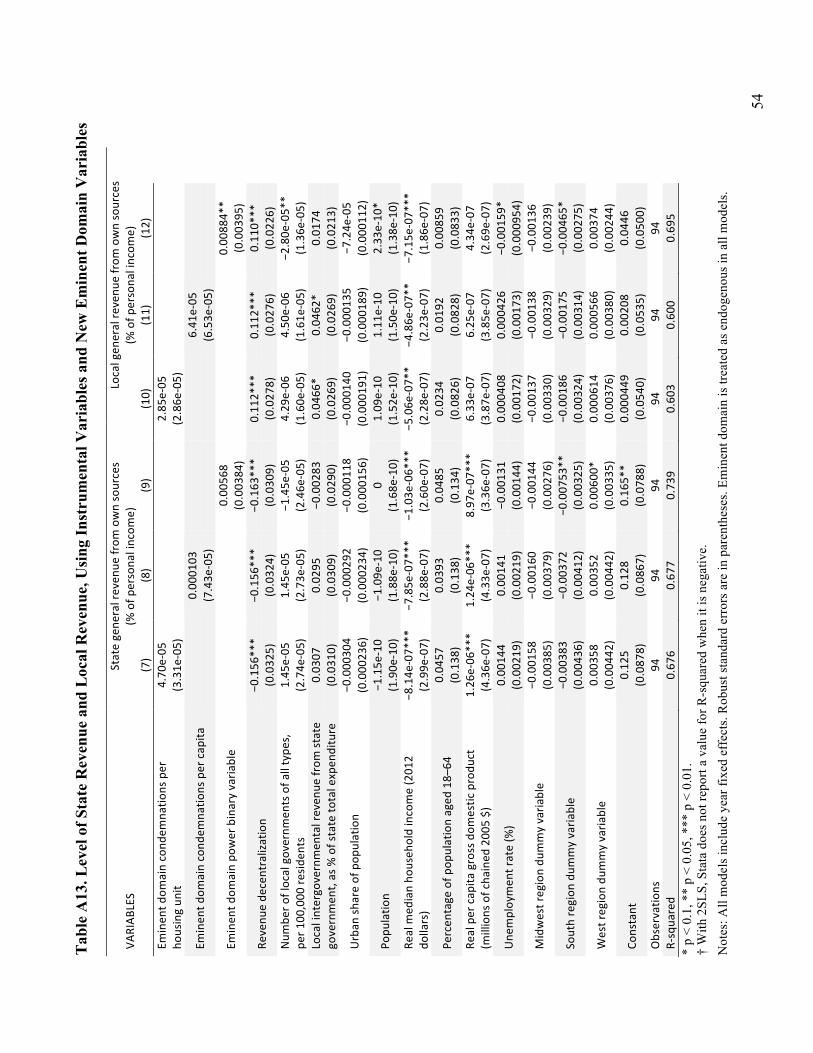
54

Tab

le A

13. L

evel

of S

tate

Rev

enue

and

Loc

al R

even

ue, U

sing

Inst

rum

enta

l Var

iabl

es a

nd N

ew E

min

ent D

omai

n V

aria

bles

VARIAB

LES  

State  gene

ral  reven

ue  from

 own  sources  

(%  of  p

ersona

l  incom

e)  

Local  gen

eral  re

venu

e  from

 own  sources  

(%  of  p

ersona

l  incom

e)  

(7)  

(8)  

(9)  

(10)  

(11)  

(12)  

Eminen

t  dom

ain  cond

emna

tions  per    

housing  un

it  4.70

e-­‐05

   

 2.85

e-­‐05

   

 (3.31e

-­‐05)  

   

(2.86e

-­‐05)  

   

Eminen

t  dom

ain  cond

emna

tions  per  cap

ita  

 0.00

0103

   

 6.41

e-­‐05

   

 (7.43e

-­‐05)  

   

(6.53e

-­‐05)  

 Em

inen

t  dom

ain  po

wer  binary  varia

ble  

   

0.00

568  

   

0.00

884*

*  

   

(0.003

84)  

   

(0.003

95)  

Revenu

e  de

centralization  

−0.156

***  

−0.156

***  

−0.163

***  

0.11

2***  

0.11

2***  

0.11

0***  

(0.032

5)  

(0.032

4)  

(0.030

9)  

(0.027

8)  

(0.027

6)  

(0.022

6)  

Num

ber  o

f  local  governm

ents  of  a

ll  type

s,  

per  1

00,000

 resid

ents  

1.45

e-­‐05

 1.45

e-­‐05

 −1

.45e

-­‐05  

4.29

e-­‐06

 4.50

e-­‐06

 −2

.80e

-­‐05*

*  (2.74e

-­‐05)  

(2.73e

-­‐05)  

(2.46e

-­‐05)  

(1.60e

-­‐05)  

(1.61e

-­‐05)  

(1.36e

-­‐05)  

Local  intergovernmen

tal  reven

ue  from

 state  

governmen

t,  as  %  of  state  to

tal  expen

diture  

0.03

07  

0.02

95  

−0.002

83  

0.04

66*  

0.04

62*  

0.01

74  

(0.031

0)  

(0.030

9)  

(0.029

0)  

(0.026

9)  

(0.026

9)  

(0.021

3)  

Urban

 share  of  pop

ulation  

−0.000

304  

−0.000

292  

−0.000

118  

−0.000

140  

−0.000

135  

−7.24e

-­‐05  

(0.000

236)  

(0.000

234)  

(0.000

156)  

(0.000

191)  

(0.000

189)  

(0.000

112)  

Popu

latio

n  −1

.15e

-­‐10  

−1.09e

-­‐10  

0  1.09

e-­‐10

 1.11

e-­‐10

 2.33

e-­‐10

*  (1.90e

-­‐10)  

(1.88e

-­‐10)  

(1.68e

-­‐10)  

(1.52e

-­‐10)  

(1.50e

-­‐10)  

(1.38e

-­‐10)  

Real  m

edian  ho

useh

old  income  (201

2  do

llars)  

−8.14e

-­‐07*

**  

−7.85e

-­‐07*

**  

−1.03e

-­‐06*

**  

−5.06e

-­‐07*

*  −4

.86e

-­‐07*

*  −7

.15e

-­‐07*

**  

(2.99e

-­‐07)  

(2.88e

-­‐07)  

(2.60e

-­‐07)  

(2.28e

-­‐07)  

(2.23e

-­‐07)  

(1.86e

-­‐07)  

Percen

tage  of  p

opulation  aged

 18–

64  

0.04

57  

0.03

93  

0.04

85  

0.02

34  

0.01

92  

0.00

859  

(0.138

)  (0.138

)  (0.134

)  (0.082

6)  

(0.082

8)  

(0.083

3)  

Real  per  cap

ita  gross  dom

estic  produ

ct  

(millions  of  cha

ined

 200

5  $)  

1.26

e-­‐06

***  

1.24

e-­‐06

***  

8.97

e-­‐07

***  

6.33

e-­‐07

 6.25

e-­‐07

 4.34

e-­‐07

 (4.36e

-­‐07)  

(4.33e

-­‐07)  

(3.36e

-­‐07)  

(3.87e

-­‐07)  

(3.85e

-­‐07)  

(2.69e

-­‐07)  

Une

mploymen

t  rate  (%

)  0.00

144  

0.00

141  

−0.001

31  

0.00

0408

 0.00

0426

 −0

.001

59*  

(0.002

19)  

(0.002

19)  

(0.001

44)  

(0.001

72)  

(0.001

73)  

(0.000

954)  

Midwest  region  du

mmy  varia

ble  

−0.001

58  

−0.001

60  

−0.001

44  

−0.001

37  

−0.001

38  

−0.001

36  

(0.003

85)  

(0.003

79)  

(0.002

76)  

(0.003

30)  

(0.003

29)  

(0.002

39)  

South  region

 dum

my  varia

ble  

−0.003

83  

−0.003

72  

−0.007

53**  

−0.001

86  

−0.001

75  

−0.004

65*  

(0.004

36)  

(0.004

12)  

(0.003

25)  

(0.003

24)  

(0.003

14)  

(0.002

75)  

West  region  du

mmy  varia

ble  

0.00

358  

0.00

352  

0.00

600*

 0.00

0614

 0.00

0566

 0.00

374  

(0.004

42)  

(0.004

42)  

(0.003

35)  

(0.003

76)  

(0.003

80)  

(0.002

44)  

Constant  

0.12

5  0.12

8  0.16

5**  

0.00

0449

 0.00

208  

0.04

46  

(0.087

8)  

(0.086

7)  

(0.078

8)  

(0.054

0)  

(0.053

5)  

(0.050

0)  

Observatio

ns  

94  

94  

94  

94  

94  

94  

R-­‐squa

red  

0.67

6  0.67

7  0.73

9  0.60

3  0.60

0  0.69

5  *

p <

0.1,

**

p <

0.05

, ***

p <

0.0

1.

† W

ith 2

SLS,

Sta

ta d

oes n

ot re

port

a va

lue

for R

-squ

ared

whe

n it

is n

egat

ive.

N

otes

: All

mod

els i

nclu

de y

ear f

ixed

eff

ects

. Rob

ust s

tand

ard

erro

rs a

re in

par

enth

eses

. Em

inen

t dom

ain

is tr

eate

d as

end

ogen

ous i

n al

l mod

els.

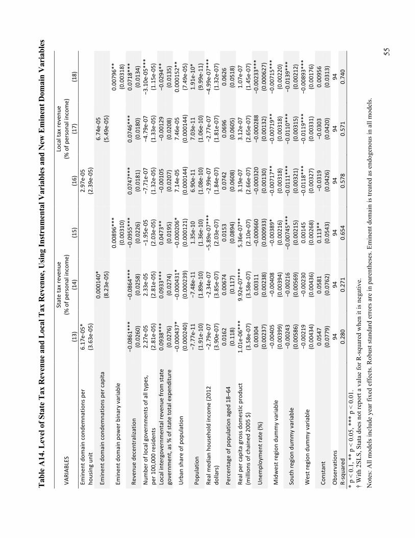
55

Tabl

e A

14. L

evel

of S

tate

Tax

Rev

enue

and

Loc

al T

ax R

even

ue, U

sing

Inst

rum

enta

l Var

iabl

es a

nd N

ew E

min

ent D

omai

n V

aria

bles

VARIAB

LES  

State  tax  revenu

e  (%

 of  p

ersona

l  incom

e)  

Local  tax  re

venu

e  (%

 of  p

ersona

l  incom

e)  

(13)  

(14)  

(15)  

(16)  

(17)  

(18)  

Eminen

t  dom

ain  cond

emna

tions  per    

housing  un

it  6.17

e-­‐05

*    

 2.97

e-­‐05

   

 (3.63e

-­‐05)  

   

(2.39e

-­‐05)  

   

Eminen

t  dom

ain  cond

emna

tions  per  cap

ita  

 0.00

0140

*    

 6.74

e-­‐05

   

 (8.23e

-­‐05)  

   

(5.49e

-­‐05)  

 Em

inen

t  dom

ain  po

wer  binary  varia

ble  

   

0.00

896*

**  

   

0.00

796*

*  

   

(0.003

10)  

   

(0.003

18)  

Revenu

e  de

centralization  

−0.086

1***  

−0.086

4***  

−0.095

5***  

0.07

47***  

0.07

46***  

0.07

18***  

(0.026

0)  

(0.025

8)  

(0.022

6)  

(0.018

1)  

(0.018

0)  

(0.013

4)  

Num

ber  o

f  local  governm

ents  of  a

ll  type

s,  

per  1

00,000

 resid

ents  

2.27

e-­‐05

 2.33

e-­‐05

 −1

.95e

-­‐05  

−7.71e

-­‐07  

−4.79e

-­‐07  

−3.10e

-­‐05*

**  

(2.81e

-­‐05)  

(2.81e

-­‐05)  

(2.03e

-­‐05)  

(1.32e

-­‐05)  

(1.33e

-­‐05)  

(1.15e

-­‐05)  

Local  intergovernmen

tal  reven

ue  from

 state  

governmen

t,  as  %  of  state  to

tal  expen

diture  

0.09

38***  

0.09

33***  

0.04

73**  

−0.001

05  

−0.001

29  

−0.029

4**  

(0.027

6)  

(0.027

4)  

(0.019

5)  

(0.020

7)  

(0.020

8)  

(0.013

5)  

Urban

 share  of  pop

ulation  

−0.000

437*

 −0

.000

431*

 −0

.000

206*

 7.14

e-­‐05

 7.46

e-­‐05

 0.00

0152

**  

(0.000

240)  

(0.000

239)  

(0.000

121)  

(0.000

144)  

(0.000

144)  

(7.49e

-­‐05)  

Popu

latio

n  −7

.77e

-­‐11  

−7.48e

-­‐11  

1.35

e-­‐10

 6.90

e-­‐11

 7.03

e-­‐11

 1.91

e-­‐10

*  (1.91e

-­‐10)  

(1.89e

-­‐10)  

(1.36e

-­‐10)  

(1.08e

-­‐10)  

(1.06e

-­‐10)  

(9.99e

-­‐11)  

Real  m

edian  ho

useh

old  income  (201

2  do

llars)  

−2.79e

-­‐07  

−2.34e

-­‐07  

−5.89e

-­‐07*

**  

−2.99e

-­‐07  

−2.77e

-­‐07  

−4.99e

-­‐07*

**  

(3.90e

-­‐07)  

(3.85e

-­‐07)  

(2.03e

-­‐07)  

(1.84e

-­‐07)  

(1.81e

-­‐07)  

(1.32e

-­‐07)  

Percen

tage  of  p

opulation  aged

 18–

64  

0.01

62  

0.00

674  

0.01

53  

0.07

42  

0.06

96  

0.06

26  

(0.118

)  (0.117

)  (0.089

4)  

(0.060

8)  

(0.060

5)  

(0.051

8)  

Real  per  cap

ita  gross  dom

estic  produ

ct  

(millions  of  cha

ined

 200

5  $)  

1.01

e-­‐06

***  

9.92

e-­‐07

***  

5.36

e-­‐07

**  

3.19

e-­‐07

 3.12

e-­‐07

 1.07

e-­‐07

 (3.58e

-­‐07)  

(3.58e

-­‐07)  

(2.10e

-­‐07)  

(2.66e

-­‐07)  

(2.65e

-­‐07)  

(1.45e

-­‐07)  

Une

mploymen

t  rate  (%

)  0.00

304  

0.00

311  

−0.000

660  

−0.000

320  

−0.000

288  

−0.002

33***  

(0.002

37)  

(0.002

38)  

(0.000

933)  

(0.001

30)  

(0.001

32)  

(0.000

627)  

Midwest  region  du

mmy  varia

ble  

−0.004

05  

−0.004

08  

−0.003

89*  

−0.007

17**  

−0.007

19**  

−0.007

15***  

(0.003

99)  

(0.003

94)  

(0.002

16)  

(0.003

18)  

(0.003

18)  

(0.002

20)  

South  region

 dum

my  varia

ble  

−0.002

43  

−0.002

16  

−0.007

45***  

−0.011

1***  

−0.011

0***  

−0.013

9***  

(0.005

86)  

(0.005

69)  

(0.002

15)  

(0.003

21)  

(0.003

15)  

(0.002

12)  

West  region  du

mmy  varia

ble  

−0.002

19  

−0.002

30  

0.00

145  

−0.011

8***  

−0.011

9***  

−0.008

93***  

(0.004

34)  

(0.004

36)  

(0.002

68)  

(0.003

27)  

(0.003

31)  

(0.001

76)  

Constant  

0.05

47  

0.05

81  

0.11

3**  

−0.031

9  −0

.030

3  0.00

956  

(0.077

9)  

(0.076

2)  

(0.054

3)  

(0.042

6)  

(0.042

0)  

(0.031

3)  

Observatio

ns  

94  

94  

94  

94  

94  

94  

R-­‐squa

red  

0.28

0  0.27

1  0.65

4  0.57

8  0.57

1  0.74

0  *

p <

0.1,

**

p <

0.05

, ***

p <

0.0

1.

† W

ith 2

SLS,

Sta

ta d

oes n

ot re

port

a va

lue

for R

-squ

ared

whe

n it

is n

egat

ive.

N

otes

: All

mod

els i

nclu

de y

ear f

ixed

eff

ects

. Rob

ust s

tand

ard

erro

rs a

re in

par

enth

eses

. Em

inen

t dom

ain

is tr

eate

d as

end

ogen

ous i

n al

l mod

els.

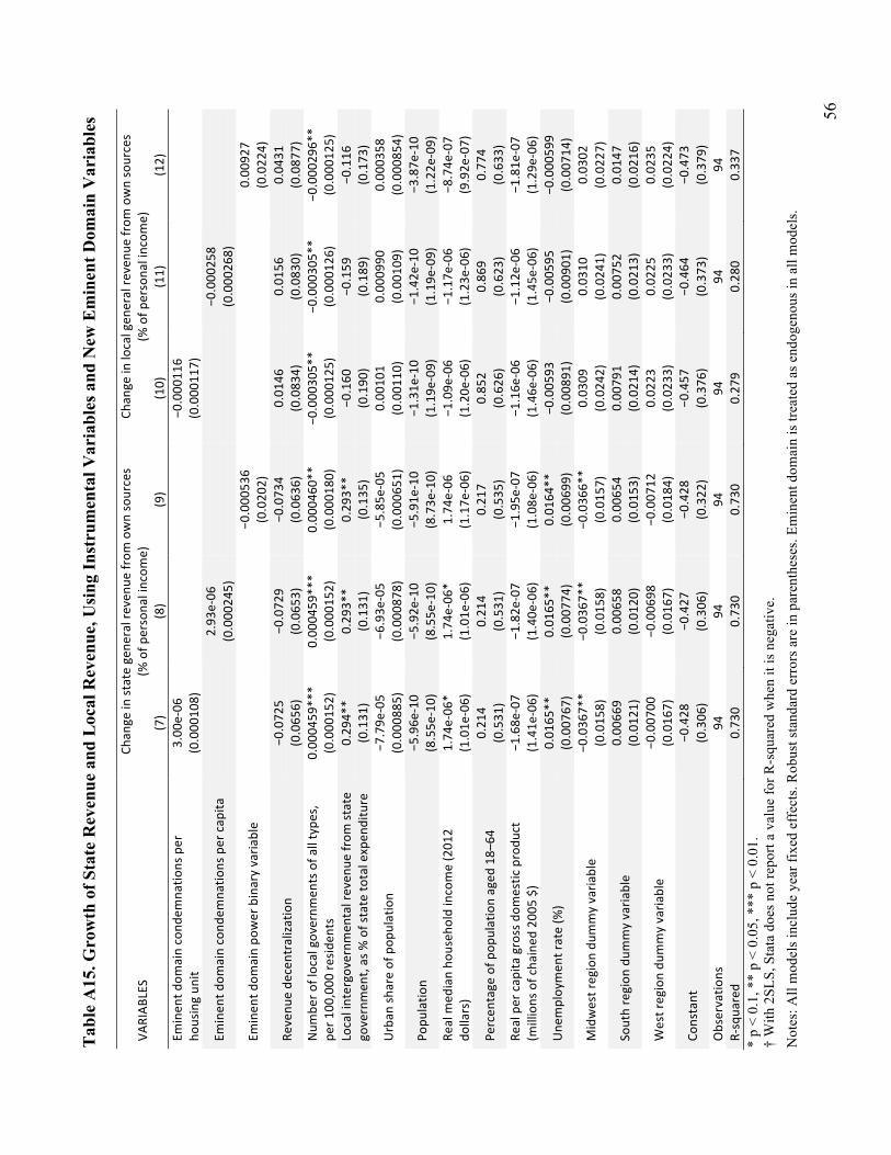
56

Tab

le A

15. G

row

th o

f Sta

te R

even

ue a

nd L

ocal

Rev

enue

, Usi

ng In

stru

men

tal V

aria

bles

and

New

Em

inen

t Dom

ain

Var

iabl

es

VARIAB

LES  

Chan

ge  in  state  gene

ral  reven

ue  from

 own  sources    

(%  of  p

ersona

l  incom

e)  

Chan

ge  in  local  gen

eral  re

venu

e  from

 own  sources  

(%  of  p

ersona

l  incom

e)  

(7)  

(8)  

(9)  

(10)  

(11)  

(12)  

Eminen

t  dom

ain  cond

emna

tions  per    

housing  un

it  3.00

e-­‐06

   

 −0

.000

116  

   

(0.000

108)  

   

(0.000

117)  

   

Eminen

t  dom

ain  cond

emna

tions  per  cap

ita  

 2.93

e-­‐06

   

 −0

.000

258  

   

(0.000

245)  

   

(0.000

268)  

 Em

inen

t  dom

ain  po

wer  binary  varia

ble  

   

−0.000

536  

   

0.00

927  

   

(0.020

2)  

   

(0.022

4)  

Revenu

e  de

centralization  

−0.072

5  −0

.072

9  −0

.073

4  0.01

46  

0.01

56  

0.04

31  

(0.065

6)  

(0.065

3)  

(0.063

6)  

(0.083

4)  

(0.083

0)  

(0.087

7)  

Num

ber  o

f  local  governm

ents  of  a

ll  type

s,  

per  1

00,000

 resid

ents  

0.00

0459

***  

0.00

0459

***  

0.00

0460

**  

−0.000

305*

*  −0

.000

305*

*  −0

.000

296*

*  (0.000

152)  

(0.000

152)  

(0.000

180)  

(0.000

125)  

(0.000

126)  

(0.000

125)  

Local  intergovernmen

tal  reven

ue  from

 state  

governmen

t,  as  %  of  state  to

tal  expen

diture  

0.29

4**  

0.29

3**  

0.29

3**  

−0.160

 −0

.159

 −0

.116

 (0.131

)  (0.131

)  (0.135

)  (0.190

)  (0.189

)  (0.173

)  

Urban

 share  of  pop

ulation  

−7.79e

-­‐05  

−6.93e

-­‐05  

−5.85e

-­‐05  

0.00

101  

0.00

0990

 0.00

0358

 (0.000

885)  

(0.000

878)  

(0.000

651)  

(0.001

10)  

(0.001

09)  

(0.000

854)  

Popu

latio

n  −5

.96e

-­‐10  

−5.92e

-­‐10  

−5.91e

-­‐10  

−1.31e

-­‐10  

−1.42e

-­‐10  

−3.87e

-­‐10  

(8.55e

-­‐10)  

(8.55e

-­‐10)  

(8.73e

-­‐10)  

(1.19e

-­‐09)  

(1.19e

-­‐09)  

(1.22e

-­‐09)  

Real  m

edian  ho

useh

old  income  (201

2  do

llars)  

1.74

e-­‐06

*  1.74

e-­‐06

*  1.74

e-­‐06

 −1

.09e

-­‐06  

−1.17e

-­‐06  

−8.74e

-­‐07  

(1.01e

-­‐06)  

(1.01e

-­‐06)  

(1.17e

-­‐06)  

(1.20e

-­‐06)  

(1.23e

-­‐06)  

(9.92e

-­‐07)  

Percen

tage  of  p

opulation  aged

 18–

64  

0.21

4  0.21

4  0.21

7  0.85

2  0.86

9  0.77

4  (0.531

)  (0.531

)  (0.535

)  (0.626

)  (0.623

)  (0.633

)  Re

al  per  cap

ita  gross  dom

estic  produ

ct  

(millions  of  cha

ined

 200

5  $)  

−1.68e

-­‐07  

−1.82e

-­‐07  

−1.95e

-­‐07  

−1.16e

-­‐06  

−1.12e

-­‐06  

−1.81e

-­‐07  

(1.41e

-­‐06)  

(1.40e

-­‐06)  

(1.08e

-­‐06)  

(1.46e

-­‐06)  

(1.45e

-­‐06)  

(1.29e

-­‐06)  

Une

mploymen

t  rate  (%

)  0.01

65**  

0.01

65**  

0.01

64**  

−0.005

93  

−0.005

95  

−0.000

599  

(0.007

67)  

(0.007

74)  

(0.006

99)  

(0.008

91)  

(0.009

01)  

(0.007

14)  

Midwest  region  du

mmy  varia

ble  

−0.036

7**  

−0.036

7**  

−0.036

6**  

0.03

09  

0.03

10  

0.03

02  

(0.015

8)  

(0.015

8)  

(0.015

7)  

(0.024

2)  

(0.024

1)  

(0.022

7)  

South  region

 dum

my  varia

ble  

0.00

669  

0.00

658  

0.00

654  

0.00

791  

0.00

752  

0.01

47  

(0.012

1)  

(0.012

0)  

(0.015

3)  

(0.021

4)  

(0.021

3)  

(0.021

6)  

West  region  du

mmy  varia

ble  

−0.007

00  

−0.006

98  

−0.007

12  

0.02

23  

0.02

25  

0.02

35  

(0.016

7)  

(0.016

7)  

(0.018

4)  

(0.023

3)  

(0.023

3)  

(0.022

4)  

Constant  

−0.428

 −0

.427

 −0

.428

 −0

.457

 −0

.464

 −0

.473

 (0.306

)  (0.306

)  (0.322

)  (0.376

)  (0.373

)  (0.379

)  Observatio

ns  

94  

94  

94  

94  

94  

94  

R-­‐squa

red  

0.73

0  0.73

0  0.73

0  0.27

9  0.28

0  0.33

7  *

p <

0.1,

**

p <

0.05

, ***

p <

0.0

1.

† W

ith 2

SLS,

Sta

ta d

oes n

ot re

port

a va

lue

for R

-squ

ared

whe

n it

is n

egat

ive.

N

otes

: All

mod

els i

nclu

de y

ear f

ixed

eff

ects

. Rob

ust s

tand

ard

erro

rs a

re in

par

enth

eses

. Em

inen

t dom

ain

is tr

eate

d as

end

ogen

ous i

n al

l mod

els.

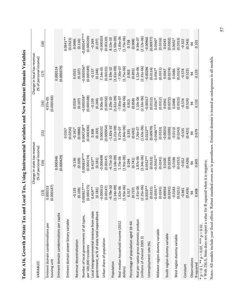
57

Tab

le A

16. G

row

th o

f Sta

te T

ax a

nd L

ocal

Tax

, Usi

ng In

stru

men

tal V

aria

bles

and

New

Em

inen

t Dom

ain

Var

iabl

es

VARIAB

LES  

Chan

ge  in  state  tax  revenu

e  (%

 of  p

ersona

l  incom

e)  

Chan

ge  in  local  tax  re

venu

e  (%

 of  p

ersona

l  incom

e)  

(13)  

(14)  

(15)  

(16)  

(17)  

(18)  

Eminen

t  dom

ain  cond

emna

tions  per    

housing  un

it  0.00

0153

   

 4.97

e-­‐05

   

 (0.000

187)  

   

(0.000

166)  

   

Eminen

t  dom

ain  cond

emna

tions  per  cap

ita  

 0.00

0346

   

 0.00

0124

   

 (0.000

429)  

   

(0.000

379)  

 Em

inen

t  dom

ain  po

wer  binary  varia

ble  

   

0.01

67  

   

0.06

41**  

   

(0.025

6)  

   

(0.032

3)  

Revenu

e  de

centralization  

−0.135

 −0

.136

 −0

.161

*  0.03

24  

0.03

31  

0.04

86  

(0.109

)  (0.109

)  (0.088

6)  

(0.107

)  (0.107

)  (0.116

)  Num

ber  o

f  local  governm

ents  of  a

ll  type

s,  

per  1

00,000

 resid

ents  

0.00

0817

***  

0.00

0819

***  

0.00

0728

**  

−0.000

358*

 −0

.000

356*

 −0

.000

547*

**  

(0.000

275)  

(0.000

274)  

(0.000

306)  

(0.000

188)  

(0.000

189)  

(0.000

200)  

Local  intergovernmen

tal  reven

ue  from

 state  

governmen

t,  as  %  of  state  to

tal  expen

diture  

0.41

4**  

0.41

3**  

0.30

8  −0

.139

 −0

.137

 −0

.269

 (0.181

)  (0.181

)  (0.193

)  (0.244

)  (0.244

)  (0.197

)  

Urban

 share  of  pop

ulation  

−0.000

515  

−0.000

498  

0.00

0102

 9.00

e-­‐05

 7.14

e-­‐05

 −0

.000

203  

(0.001

47)  

(0.001

47)  

(0.000

954)  

(0.001

56)  

(0.001

55)  

(0.001

20)  

Popu

latio

n  −6

.78e

-­‐10  

−6.71e

-­‐10  

−1.82e

-­‐10  

3.29

e-­‐10

 3.19

e-­‐10

 8.13

e-­‐10

 (1.14e

-­‐09)  

(1.14e

-­‐09)  

(1.21e

-­‐09)  

(1.61e

-­‐09)  

(1.61e

-­‐09)  

(1.50e

-­‐09)  

Real  m

edian  ho

useh

old  income  (201

2  do

llars)  

1.62

e-­‐06

 1.73

e-­‐06

 9.27

e-­‐07

 −7

.85e

-­‐07  

−7.30e

-­‐07  

−1.83e

-­‐06  

(1.93e

-­‐06)  

(1.91e

-­‐06)  

(1.84e

-­‐06)  

(1.68e

-­‐06)  

(1.75e

-­‐06)  

(1.73e

-­‐06)  

Percen

tage  of  p

opulation  aged

 18–

64  

0.31

7  0.29

4  0.33

1  0.91

3  0.90

3  0.73

8  (0.737

)  (0.741

)  (0.692

)  (0.858

)  (0.855

)  (0.908

)  Re

al  per  cap

ita  gross  dom

estic  produ

ct  

(millions  of  cha

ined

 200

5  $)  

1.91

e-­‐06

 1.87

e-­‐06

 7.26

e-­‐07

 1.10

e-­‐06

 1.12

e-­‐06

 9.34

e-­‐07

 (2.35e

-­‐06)  

(2.34e

-­‐06)  

(1.63e

-­‐06)  

(2.33e

-­‐06)  

(2.31e

-­‐06)  

(2.12e

-­‐06)  

Une

mploymen

t  rate  (%

)  0.03

10**  

0.03

12**  

0.02

22**  

−0.003

17  

−0.002

86  

−0.009

66  

(0.012

1)  

(0.012

2)  

(0.009

79)  

(0.011

2)  

(0.011

4)  

(0.009

77)  

Midwest  region  du

mmy  varia

ble  

−0.059

1**  

−0.059

2**  

−0.058

6***  

0.05

67*  

0.05

67*  

0.05

60*  

(0.024

1)  

(0.024

1)  

(0.022

3)  

(0.031

2)  

(0.031

1)  

(0.031

6)  

South  region

 dum

my  varia

ble  

0.00

934  

0.01

00  

−0.002

52  

0.03

41  

0.03

47  

0.02

43  

(0.024

1)  

(0.023

9)  

(0.020

0)  

(0.027

2)  

(0.027

4)  

(0.030

2)  

West  region  du

mmy  varia

ble  

−0.018

3  −0

.018

6  −0

.011

0  0.04

88  

0.04

86  

0.06

92*  

(0.025

1)  

(0.025

2)  

(0.024

3)  

(0.032

3)  

(0.032

4)  

(0.035

3)  

Constant  

−0.661

 −0

.652

 −0

.535

 −0

.574

 −0

.574

 −0

.322

 (0.426

)  (0.426

)  (0.421

)  (0.524

)  (0.522

)  (0.543

)  Observatio

ns  

94  

94  

94  

94  

94  

94  

R-­‐squa

red  

0.60

8  0.60

5  0.67

9  0.13

2  0.13

3  0.10

1  *

p <

0.1,

**

p <

0.05

, ***

p <

0.0

1.

† W

ith 2

SLS,

Sta

ta d

oes n

ot re

port

a va

lue

for R

-squ

ared

whe

n it

is n

egat

ive.

N

otes

: All

mod

els i

nclu

de y

ear f

ixed

eff

ects

. Rob

ust s

tand

ard

erro

rs a

re in

par

enth

eses

. Em

inen

t dom

ain

is tr

eate

d as

end

ogen

ous i

n al

l mod

els.