Technical report on model development Representing finance

Technical report on model development – Representing

finance constraints in a post-

Keynesian macro-sectoral

model

Technical Study on the Macroeconomics of Energy and Climate Policies

Representing finance constraints in a post-Keynesian macro-sectoral model

February 2017 ii

Prepared by

Richard Lewney, Cambridge Econometrics

Unnada Chewpreecha, Cambridge Econometrics

Hector Pollitt, Cambridge Econometrics

Contact:

Richard Lewney

Cambridge Econometrics Ltd,

Covent Garden

Cambridge, UK

CB1 2HT

Rue Belliard 15-17

1040 Brussels

[email protected]

Tel: +44 1223 533100

This study was ordered and paid for by the European Commission, Directorate-

General for Energy, Contract no. ENER/A4/2015-436/SER/S12.716128. The

information and views set out in this study are those of the author(s) and do not

necessarily reflect the official opinion of the Commission. The Commission does not

guarantee the accuracy of the data included in this study. Neither the Commission

nor any person acting on the Commission’s behalf may be held responsible for the

use which may be made of the information contained therein.

© European Union, September 2017

Reproduction is authorised provided the source is acknowledged.

More information on the European Union is available at http://europa.eu.

mailto:[email protected]


February 2017 iii

Table of Contents

Part I. Introduction ........................................................................................................ 1

Part II. Developing the theoretical design ..................................................... 2

Part III. Making the design operational in an empirical model ....... 7

Part IV. Modelling macro confidence effects on the interest rate faced by borrowers .............................................................................................. 10

Part V. Incorporating the private commercial rate and estimated sector debt in E3ME’s investment equations .................... 18


June 2017 1

Part I. Introduction

This document describes the thinking and implementation of an explicit treatment

of finance constraints for decarbonisation (and other) investments in a post-

Keynesian macro-sectoral1 model, exemplified here by the Cambridge

Econometrics’ E3ME energy-economy-environment model.

In many cases, the changes required to decarbonise the economy involve a

substitution of capital for fossil fuel energy use. Examples include the use of

renewable technologies in centralised or decentralised power generation, or the use

of electricity in domestic heating or road transport, all of which entail an up-front

capital expenditure in return for the elimination of current fossil fuel energy inputs.

Except for small-scale projects, typically the agent may not be able to, or choose

to, finance the capital expenditure out of their existing income or stock of savings:

the question therefore arises as to whether financial capital will be made available

by lenders and on what terms and, if this is likely to become an important obstacle

to investment, whether policy action can facilitate a larger flow of financial capital

to support the transition. It therefore becomes particularly important to represent

the factors determining the availability of finance explicitly in economic modelling.

Post-Keynesian theory is characterised by the assumption that money is created

endogenously by commercial banks rather than controlled by central banks or

constrained by the availability of saving (the surplus of income over consumption)

by the various agents in the economy. This report describes the approach taken to

implement an explicit treatment of finance in an empirical post-Keynesian macro

sectoral model.

The structure of the document is as follows. Part II discusses the theoretical design

and Part III the issues involved in making this design operational. Part IV reviews

empirical evidence for the cost of borrowing faced by commercial borrowers and

presents the econometric equations estimated to determine that commercial rate in

E3ME. Part V discusses the effect of including this commercial rate of interest and

a debt burden term in E3ME’s investment equations and conducts some stylised

simulations to show the difference that the new specification makes.

1 ‘Macro-sectoral’ here means a whole-economy model with macroeconomic aggregates and sectoral (industry/product) detail. Such models are less common than pure macroeconomic models, but sectoral detail is essential for analysis of the kind of structural economic change associated a shift from dependence on fossil fuels.


June 2017 2

Part II. Developing the theoretical design This section develops the logic of what we seek to capture in the empirical model.

It begins with a description of the logic of a post-Keynesian model that does not

explicitly recognise finance constraints, and then extends this to incorporate

explicitly the constraints that earlier work in the project has identified.

Determination of investment in a post-Keynesian model without explicit

representation of finance constraints

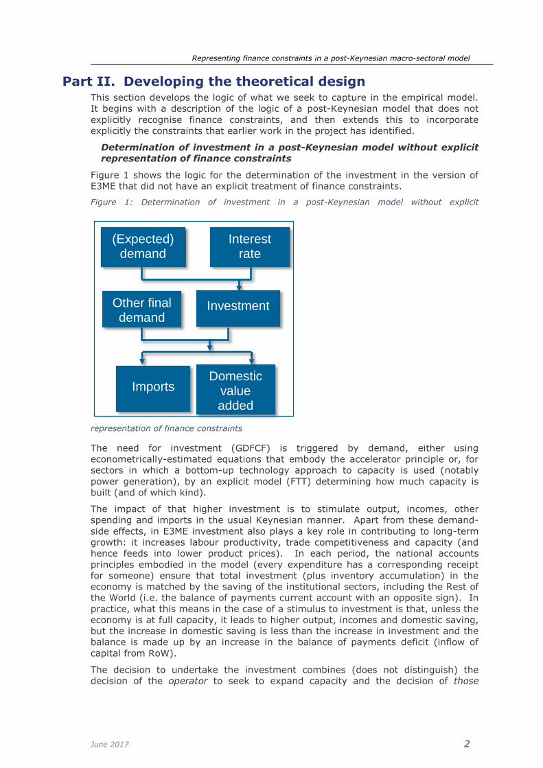
Figure 1 shows the logic for the determination of the investment in the version of

E3ME that did not have an explicit treatment of finance constraints.

Figure 1: Determination of investment in a post-Keynesian model without explicit

representation of finance constraints

The need for investment (GDFCF) is triggered by demand, either using

econometrically-estimated equations that embody the accelerator principle or, for

sectors in which a bottom-up technology approach to capacity is used (notably

power generation), by an explicit model (FTT) determining how much capacity is

built (and of which kind).

The impact of that higher investment is to stimulate output, incomes, other

spending and imports in the usual Keynesian manner. Apart from these demand-

side effects, in E3ME investment also plays a key role in contributing to long-term

growth: it increases labour productivity, trade competitiveness and capacity (and

hence feeds into lower product prices). In each period, the national accounts

principles embodied in the model (every expenditure has a corresponding receipt

for someone) ensure that total investment (plus inventory accumulation) in the

economy is matched by the saving of the institutional sectors, including the Rest of

the World (i.e. the balance of payments current account with an opposite sign). In

practice, what this means in the case of a stimulus to investment is that, unless the

economy is at full capacity, it leads to higher output, incomes and domestic saving,

but the increase in domestic saving is less than the increase in investment and the

balance is made up by an increase in the balance of payments deficit (inflow of

capital from RoW).

The decision to undertake the investment combines (does not distinguish) the

decision of the operator to seek to expand capacity and the decision of those

(Expected) demand

Imports Domestic

value added

Interest rate

Investment Other final demand


June 2017 3

financing the investment that the risk-return ratio is satisfactory. The investment

equation includes the interest rate but this has often not shown up as

econometrically or economically significant, because year-on-year variation in

investment is dominated by short-term cyclical effects and because the observable

interest rate is the central bank short-term rate rather than the rate charged by

commercial banks.

Apart from whatever is included in the investment equation, there is no ‘financing

constraint’: under the usual post-Keynesian assumption of endogenous money,

banks are assumed to create the credit to finance the transaction and the amount

of saving undertaken in a given year by domestic institutions does not constrain

investment in that year (because it does not constrain bank lending).

There could, in principle, be a short-term, real-economy capacity constraint on

production of investment goods if the economy is operating at full capacity, in

which case the attempt to spend more on investment will result in the model in

higher inflation, including in the prices of investment goods (so that the real-terms

equivalent of any given current-price level of investment is reduced), a reduction in

other final demand (for example, because consumption prices are higher) and an

increase in imports.

Developing the logic of an explicit representation of finance constraints

Finance constraints are relevant for all kinds of investment decision. Because the

changes required to decarbonise the economy commonly involve a substitution of

capital for fossil fuel energy use, finance constraints upon investment that slow the

pace of that substitution are of particular interest in the context of decarbonisation

policy. Different kinds of agents (for example, large companies on the one hand

and households or small businesses on the other) face different kinds of finance

constraints and have particular roles to play in any plausible pathway to a

decarbonised economy.

In post-Keynesian theory, an economy’s capacity to take on risk for investment (or

the willingness of its agents to do so, or the willingness of the rest of the world to

invest in the country) depends on the net wealth and gearing of its agents, not on

the saving that happens to be carried out in the current year. For example, an

agent that has built up substantial net financial wealth from past saving, and which

is carrying little debt, can commit funds to a new investment project without much

threat to its solvency. But an agent with low net financial wealth faces a larger risk

of insolvency if it commits a large part of that wealth or takes on debt to invest in a

new project. Similarly, an agent with moderate net financial wealth but with

substantial debt (more than balanced by substantial assets), and therefore a high

debt service to income ratio, can only invest in a new project by using some of its

financial wealth or by increasing its debt, exposing it to a greater risk of insolvency.

In boom times, when asset prices are rising and new investments are expected to

be successful, the agent may regard the risk of failure as low and so be willing to

commit to a new project; similarly, financial investors will be more willing to

commit funds in that kind of environment.

If the regulatory environment changes to allow insurance companies and pension

funds to invest more in infrastructure assets, this makes available to the

infrastructure operators a capacity to invest in this asset type (the strong balance

sheet of the insurance companies and pension funds (ICPFs)) that was not

previously available. That is then reflected in a lower cost of capital for the

infrastructure operator (and a greater willingness of the financial community to

make finance available).

In post-Keynesian theory, the potential supply of finance capital in a given year is

not the same as (or determined by) the level of ‘saving’ (the difference between


June 2017 4

income and consumption for each institutional sector in any year). For institutions

other than banks, the potential supply of finance capital depends on their stock of

financial assets, their saving in the present year, and their willingness and capacity

to borrow from banks to commit to a project. Endogenous money means that the

level of saving in a given year is not closely related to the potential supply of

finance capital: during a boom, saving may be low while at the same time banks

are expanding their balance sheet, whereas during a recession the opposite may be

true. The net result of these decisions and the outcomes for income and spending

in the economy will determine the balance of saving and investment in the

economy in any given year and the net inflow or outflow of capital from abroad.

When an investment project is undertaken, the operator needs to raise finance to

cover the cost of the investment. When the investment expenditure occurs, the

balance sheet of the project’s operator shows an increase in real assets (the

investment in fixed capital), an increase in financial liabilities (the new debt or in

equity provided by other agents) and a reduction in financial assets (the own funds

contributed by the operator).

Corresponding to that supply of financial instruments are entries on the asset and

liabilities accounts for the financing institutions. For banks the additional asset is

the new loan to the operator and the additional liability is a corresponding increase

in bank deposits. For a financial institution (say, a pension fund) subscribing to a

bond or equity issue, the additional asset is the bond or equity holding and the

liability is a reduction in holdings of other financial assets (for example, bank

deposits). Most households do not invest directly in projects (other than the

investments by owner-occupiers in their own homes), but rather put their saving

into pension funds, insurance companies and investment funds.

Figure 2 shows the logic of a theoretical post-Keynesian model that has been

extended to make explicit the role of financial constraints. The effect of the

extension is to incorporate:

the macroeconomic conditions that affect the risk environment for investment,

notably distinguishing the role of the (short-term) policy interest rate set by the

central bank from the (long-term) rate at which lenders make finance available

to borrowers; regulatory changes also play a role, typically affecting the

distribution of finance across alternative asset classes

the project-specific factors that raise the cost / reduce the availability of finance

for riskier projects: these would not be distinguished in a purely macroeconomic

model, but can be made explicit in a macro-sectoral model that distinguishes

different (for example, more or less carbon-intensive) sectors and technologies

the scale of indebtedness of the borrower, which increases the risk of failure

and default

Hence, Figure 2 shows that the cost of capital to the project operator (e.g. a power

generation utility company) depends on:

the expected return on the project (because a high expected return provides a

cushion to absorb unexpected negative factors)

the risk (and other) characteristics of the project

the credit risk of the project operator

the macroeconomic cost of finance capital

With regard to the perceived risk (and other) characteristics of the project, these

incorporate:


June 2017 5

country risk: all the factors that make the risk of default or disappointing

returns higher in some countries than others for any kind of project

project/technology risk: factors specific to the type of project (e.g. the risk of

construction cost overruns; the risk that the technology performs less well than

expected; performance risk, design risk, operation and maintenance risk; the

time period required for the capital cost to be recovered; the likely price at

which the operator’s product can be sold in future)

policy risk: the risk that a change in policy will lower the project’s returns in

future (so, the extent to which the project’s success depends on policy, and the

credibility of commitments to maintain or strengthen the policy regime)

borrower risk: the borrower’s credit-worthiness (track record, existing gearing)

scale of project: this affects the administrative overhead for the financial

institution; for some kinds of finance, projects have to be larger than a certain

minimum size (or, perhaps, aggregated into bundles that exceed the minimum

size)

the value of collateral (which depends on whether there is a liquid market for

the asset on which the loan has been secured)

With regard to the macroeconomic supply-side drivers of the cost of capital, these

include:

the costs to banks of raising finance to lend directly to project operators or

indirectly (by providing loans to investment banks seeking to gear up to invest

in projects): the central bank lending rate, the prudential regulatory regime

with regard to bank capital (equity), structural changes that give banks access

to cheaper sources of finance (e.g. securitisation), and the general level of

confidence which determines the cost of equity and bond finance and banks’

willingness to expand their balance sheets

prudential regulation of other financial institutions: in particular, the rules

governing the extent to which insurance companies and pension funds can

invest in this kind of project


June 2017 6

Figure 2: The logic of an explicit representation of finance constraints in a post-Keynesian model

Other financial demand

Project/ Technology/

Risk

Policy risk

Borrower risk

Country risk

Bank loans

(New) Bonds

Stock of debt (start)

Debt

repayments

Stock of debt (end)

Imports Domestic value added

Own resources

(New) Equity

(New) Debt

Financing

Macro supply-side drivers of cost of capital

Central bank interest rate

Macro confidence

Regulation

Cost of capital

to private borrowers

Cost of capital from ICPFs

(Expected)

Demand

Availability and value of

collateral

Scale of project

Characteristics of the

investment project

Project cost of capital

Investment


June 2017 7

Part III. Making the design operational in an empirical model

There are a number of issues to be overcome in making this design operational.

What we distinguish in the macro-sectoral modelling is not normally ‘a project’

undertaken by an operator, but annual investment by an industry. How then

can we represent risk characteristics that differ by type of project?

Proposed solution: In the case of power generation (the sector of most

interest), the key differences in project risk characteristics are associated with

particular technology types (how mature the technology is, how large a ‘typical’

project is). Because E3ME’s FTT:Power treatment distinguishes take-up of

different technologies in power generation), annual investment in a given

technology will correspond to one or more projects of that technology type. We

incorporate in FTT:Power assumptions for the premia associated with particular

technologies so that these are reflected in the decision made over which

technology to invest in.

We cannot observe the macro cost of capital or the project cost of capital as a

time series, and so we cannot estimate econometrically the impact of changes

in any of the determinants on the cost of capital or the impact of the cost of

capital on investment.

Proposed solution: For the macro cost of capital we use evidence from

financial market data for the interest rate on loans to commercial borrowers (or

yield on commercial bonds) and model this in relation to a ‘risk-free’ long-term

interest rate. We seek to endogenise borrower risk, making it depend on

gearing (see below on the problem of getting sufficient detail on debt by

industry sector). See Part IV below.

For the project cost of capital, and the potential role of the various project

characteristics noted in Figure 2, the disaggregation available in the model

allows us to introduce assumptions for risk premia specific to particular

countries, sectors and, for some sectors, technologies. But with the present

state of knowledge, the scale of such risk premia (and the corresponding impact

that policies designed to de-risk investments could have) would have to be

determined on a case by case basis.

What we observe is the outcome of an aggregation across heterogeneous

agents (for example, all households or all firms in an industry), so statistics

calculated for the aggregate (such as gearing) will not reflect conditions at the

tails of the distribution.

Proposed solution: We need to be aware that the level at which an

institutional sector’s gearing could constrain investment is lower than any value

that might apply to an individual borrower. This would matter if, for example,

we were attempting to represent individual projects, but we are working at the

level of sectors (and, in some cases, also technologies), not particular projects

and borrowers. Hence, in the kind of scenarios we are envisaging, we can still

use changes in the level of a statistic calculated for the aggregate as an index of

creditworthiness.


June 2017 8

We do not have data on assets/liabilities at anything more detailed than

institutional sectors so we do not have, for example, the gearing of the power

generation sector

Proposed solution: We make assumptions for the ‘typical’ extent to which

investment depends on debt (as opposed to retained profits or equity) and for

the repayment period on loans and bonds. We then construct, from historical

investment data, an estimate of the stock of loans outstanding in each year, for

each investing sector. For any given type of decarbonising investment

(according to the classification we established in an earlier report in this project2

and drawing on funding examples there), we assume that a particular mix of

sources of funds will be needed, to reflect ‘normal’ risk-sharing arrangements

(funds put in by the operator, bank loan, bonds and new equity). That mix

varies across countries according to the tradition of the country (especially bank

loans versus bonds). See Part V below. Policies that underwrite loans could be

represented by preventing the increase in gearing that would otherwise be

associated with investments.

Macro-sectoral models are sometimes used for simulations in which the take-up

of energy technologies and the resulting in change in energy use are imposed

as assumptions (drawing on the outputs of an energy system model), and the

macro-sectoral model is used solely to derive the economic implications. How

will such simulations be carried out with the extended model described here?

In this kind of simulation, since the required investment by sector and

technology is introduced by assumption from the energy system model, the

considerations set out here will largely be ignored/overwritten. However, the

energy system model may also have information about the financial incentives

that were necessary, in that model, to bring about the decision to make the

investment, and if so those incentives could be incorporated in E3ME so as to

make the simulation more complete. For example, it might be assumed in the

energy system model that a feed-in tariff guarantees the electricity price that

the investment in a particular technology will earn, in which case that

information should be incorporated in E3ME to capture the macroeconomic

impact of a higher electricity price paid by consumers.

Figure 3 summarises how these considerations have affected the operational

version of the design set out in Figure 2.

2 Trinomics (2017) Assessing the European clean energy finance landscape, with implications for improved macro-energy modelling, Deliverable D3 in the project ‘Study on the Macroeconomics of Energy and Climate Policies’.


June 2017 9

Figure 3: The operationalised representation of finance constraints in E3ME compared with the theoretical design

Other financial demand

Project/ Technology/

Risk

Policy risk

Borrower risk

Country risk

Bank loans

(New) Bonds

Stock of debt (start)

Debt repayments

Stock of debt (end)

Imports Domestic value added

Own resources

(New) Equity

(New) Debt

Financing

Macro supply-side drivers of cost of capital

Central bank interest rate

Macro confidence

Regulation

Cost of capital to private borrowers

Cost of capital from ICPFs

(Expected) Demand

Availability and value of collateral

Scale of project

Characteristics of the investment project

Project cost of capital

Investment

Not modelled

Not modelled

Scope to incorporate assumptions for risk

premia by country and sector, and for some

sectors (e.g. power) also by technology

Modelled econometrically

Improved estimate by using better macro cost of capital indicator and debt stock in econometric equations (see

Part V below)

Modelled by constructing debt estimates based on

past investment and

assumptions for loan maturities

Modelled directly in econometric

investment equations (see Part V below)


June 2017 10

Part IV. Modelling macro confidence effects on the interest rate faced by borrowers

Motivation

In this section we describe the approach taken to implement the improved

treatment of the macro supply-side drivers of the cost of capital noted in Figure 2

and Figure 4 and summarised in Part III.

Summary of the approach

E3ME includes the (short-term) policy rate and uses a Taylor rule to determine this,

but this is not an appropriate rate to use for decarbonisation investment because:

the rate of interest on loans with a long-term duration differs from the short-

term policy rate (usually higher, and less volatile over time in that it does not

rise as much when monetary policy is tightened or fall as much when it is

relaxed, because long-term inflationary expectations do not change much over

the cycle)

the rate of interest on long-term loans to the private sector includes a risk

premium which (for the average across all loans) reflects general

macroeconomic conditions; this becomes the benchmark for the rate of interest

relevant to investment (to which a premium is added that depends on the

project/borrower risk characteristics)

We therefore introduce into E3ME:

a low-risk, long-term interest rate (the yield on a safe 10-year bond, which for

countries with low sovereign credit risk is well represented by the yield on

government bonds), which acts as a benchmark for other long-term rates

an average long-term interest rate for bank loans to, or bonds sold by, the

private sector; this rate will be the default rate used for investment equations

and it is determined as a spread relative to the low-risk, long-term interest rate

Rationale and evidence

The policy rate and the long-term, low-risk rate

We assume a liquidity-preference explanation of the term structure of interest

rates: lenders are risk-averse and prefer the flexibility, in the face of uncertainty,

offered by short-term maturities; they therefore require a premium to lend for the

long term. Borrowers prefer the certainty of a long-term commitment and are

willing to pay a premium for this. The result is a rising yield curve (as the maturity

length increases). The implication is that an investor strategy of ‘buy and hold’

delivers a higher return than ‘buy short-term and continually roll over’, because the

latter strategy has the co-benefit of greater liquidity (as a hedge against

uncertainty).

However, expectations of future (short-term) interest rates also play a part. If

(short-term) interest rates are expected to fall in the future, the expected returns

on a ‘buy short-term and roll over’ strategy are less than what would be implied if

the present short-term interest rate were assumed to continue indefinitely. The

consequence is that if (short-term) interest rates are expected to fall, the gap

between the short-term and long-term rates will be lower (compared to the case

when short-term interest rates are neither expected to fall nor rise), and in extreme

circumstances the gap can be negative (the yield curve becomes inverted).

Expectations may change even if the policy rate does not change, for example if


June 2017 11

there is a shift in expectations about the long-term inflation rate: lower inflation in

the long term will be interpreted as resulting in lower nominal interest rates (for the

same real rate).

There is, therefore, a general tendency for a change in the short-term policy rate to

affect long-term rates in the same direction, but not by as much (the gap closes

when rates rise and opens when rates fall) if the new rate is perceived to be only

temporarily high or low. In practice this means that when the policy rate is raised

to curb excessive inflation (and an economic boom), the safe long-term rate does

not rise by as much (the spread between them falls); when it is cut sharply to

mitigate a recession, the safe long-term rate does not fall by as much (the spread

rises).

A third factor is the role of macroeconomic uncertainty. When conditions are

uncertain, there is a flight to safety (an increase in liquidity preference). This will

tend to increase the slope of the yield curve (the spread between short and long-

term rates). When confidence is high, the reverse is true3.

Figure 4 shows the short-term policy rate and the yield on 10-year government

bonds (interpreted as the safe benchmark asset) in the euro area (with the German

bund representing the relevant government bond), the US, the UK and Japan.

The aggressiveness of monetary policy in response to the boom and subsequent

crisis varied across the four areas (the largest changes were in the US, and the

smallest in Japan). In all cases, the spread between the policy short-term rate and

the long-term safe rate narrowed when the policy rate was increased sharply

through 2007 and 2008 and then widened when the policy rate was cut sharply in

2008 and 2009.

However, the behaviour since 2010 varies. In the euro area and to a lesser extent

the UK, the policy rate has been very low and yet the spread has narrowed sharply.

This may be partly because expectations about future (short-term) interest rates

have fallen: the expected timing and speed of a ‘return to normal’ for the policy

rate has been pushed back, so that a significant part of the 10-year period of the

bond’s maturity is now expected to be a low (policy) rate period. But it also no

doubt reflects the impact of quantitative easing (QE) which has succeeded in

driving down yields on high quality long-term securities. It is also possible that the

mood of uncertainty has eased: GDP growth is stable even if it is slow (this is

reflected in an improved ‘economic sentiment’ confidence indicator), and so

investors are less fearful of a sharp fall in asset prices4.

In the US, the reduction in the spread has been much less pronounced, which may

reflect an expectation that the policy rate will be raised sooner (than in Europe).

The case of Japan seems to be dominated by the expectation (based on historical

experience) of very low or negative inflation.

3 It is also the case that greater uncertainty will increase the spread between the rate charged on loans to (or the yield on bonds issued by) institutions whose default risk is not negligible compared with the rate for the benchmark safe asset (normally government bills/bonds), but this is a separate issue discussed in the next section).

4 Not shown in this chart, the yield spread relative to the German bund for Euro area government bonds that were perceived to be riskier rose in the crisis (most obviously for Greece, but also to a lesser extend for Ireland, Spain and Italy).


June 2017 12

The long-term low-risk rate and the rate charged to private borrowers

Because private borrowers (usually) carry a higher default risk than governments,

their loans/bonds carry an additional premium, and different borrowers/projects

carry different premia depending on the perceived risk (including the availability of

collateral to mitigate the lender’s risk). But QE can also bring down the yield on

lower quality long-term assets as investors respond to a low-interest-rate

environment by ‘reaching for yield’ (i.e. fund managers pursue higher returns by

taking on a higher level of risk than the ultimate fund owners intend).

Figure 5 shows that the yield on AAA and BAA bonds in the US has generally

followed the downward trend in the yield on government bonds in the period since

2010. It also shows the effect of the flight to safety in 2009, when the spread

increased for AAA bonds and even more sharply for BAA bonds.

Notes: The 10-year government bond rate for the Euro area is the German bund. Sources: ECB, Federal Reserve Bank of St Louis (FRED), Bank of England.

Figure 4: The short-term policy rate and the yield on 10-year government bonds in selected countries


June 2017 13

Figure 6 is intended to provide comparable information for the Euro area and the

UK, using bank loan rates. However, the long time series is only available for loans

of a shorter duration period than the 10 years needed for comparability with the

government bond rate. Hence, in the case of the Euro area, the time profile of the

commercial loan rate < 1-year is similar to the policy short-term rate. Figure 6

also shows that (for the Euro area, for which we have data) loans with an interest

rate fixed for 10 years have a higher rate than those with a rate fixed for up to a

year (so, closer to a floating rate loan), reflecting the interest rate risk borne by the

lender in the case of the longer fixed-rate period.

In the Euro area, the long-term bank loan rate has followed the government bond

yield down. This is not the case for the bank loan rate shown in the UK, which has

remained broadly stable.

Figure 5: The spread between commercial bonds of different grades and government bond yields

Source: Federal Reserve Bank of St Louis (FRED).

Figure 6: Bank loan rates and government bond yields in the Euro area and the UK

Source: European Central Bank, Bank of England.


June 2017 14

Implementation

The long-term risk free rate

Ideally, for each country we would estimate an equation which determines the 10-

year government bond yield on the basis of current and lagged values of the short-

term policy rate (interpreted as a rule for forming expectations of future short-term

rates, and hence a predictor of the 10-year government bond yield, capturing the

relationship shown in Figure 4). However, adequate time series data are not

available for every country over the long term and, for some countries, the 10-year

government bond yield includes a substantial sovereign credit risk element, which

we want to exclude at this stage.

The approach taken for the EU is to treat the German bund as the representative

long-term risk free rate and to estimate a relationship with current and lagged

values of the ECB policy interest rate. This relationship (the extent to which the

long-term risk free rate responds to changes in the policy rate) is then assumed to

apply to all countries, whether or not they are in the Euro area.

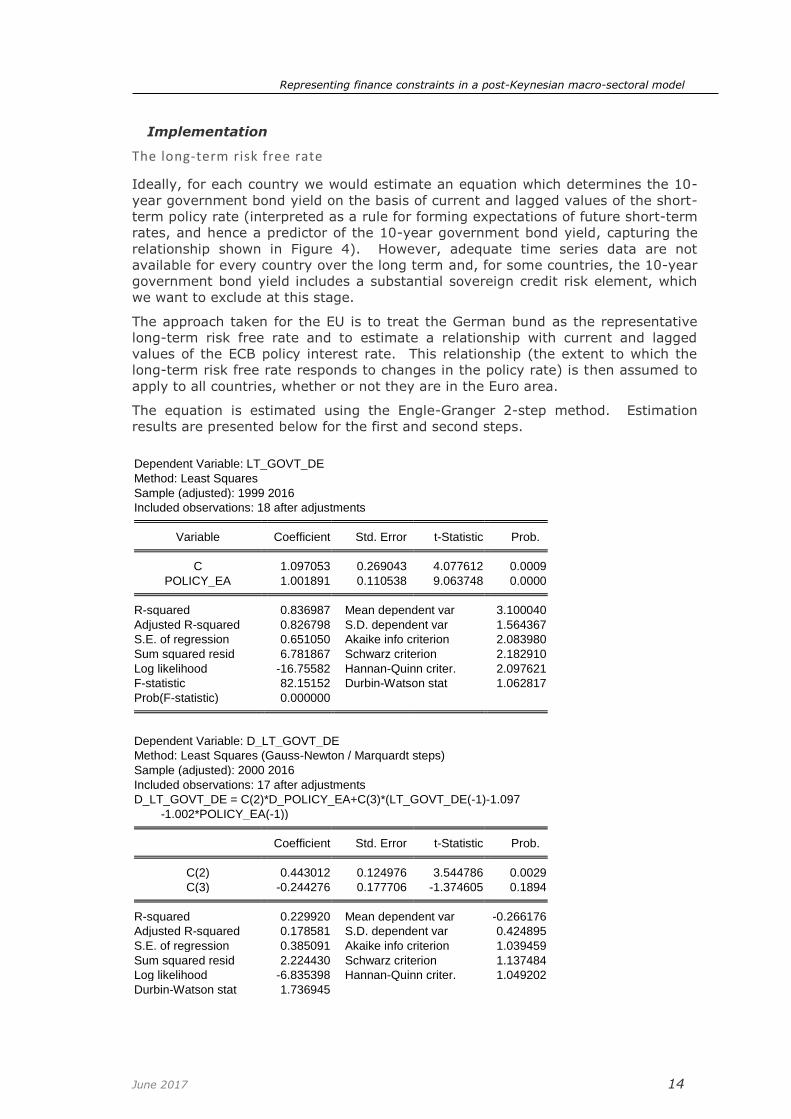
The equation is estimated using the Engle-Granger 2-step method. Estimation

results are presented below for the first and second steps.

Dependent Variable: LT_GOVT_DE

Method: Least Squares

Sample (adjusted): 1999 2016

Included observations: 18 after adjustments Variable Coefficient Std. Error t-Statistic Prob. C 1.097053 0.269043 4.077612 0.0009

POLICY_EA 1.001891 0.110538 9.063748 0.0000 R-squared 0.836987 Mean dependent var 3.100040

Adjusted R-squared 0.826798 S.D. dependent var 1.564367

S.E. of regression 0.651050 Akaike info criterion 2.083980

Sum squared resid 6.781867 Schwarz criterion 2.182910

Log likelihood -16.75582 Hannan-Quinn criter. 2.097621

F-statistic 82.15152 Durbin-Watson stat 1.062817

Prob(F-statistic) 0.000000

Dependent Variable: D_LT_GOVT_DE

Method: Least Squares (Gauss-Newton / Marquardt steps)


Included observations: 17 after adjustments

D_LT_GOVT_DE = C(2)*D_POLICY_EA+C(3)*(LT_GOVT_DE(-1)-1.097

-1.002*POLICY_EA(-1)) Coefficient Std. Error t-Statistic Prob. C(2) 0.443012 0.124976 3.544786 0.0029

C(3) -0.244276 0.177706 -1.374605 0.1894 R-squared 0.229920 Mean dependent var -0.266176





Durbin-Watson stat 1.736945


June 2017 15

LT_GOVT_DE German 10-year bund yield POLICY_EA ECB short-term policy interest rate C Constant (intercept) term D_ the one-year difference in the variable

The estimated parameters give the resulting dynamic equation the following

properties:

in the short run, a 1 pp change in the ECB policy rate leads to a 0.44 pp change

in the 10-year bund yield

in the long run, a 1 pp change in the ECB policy rate is matched by a 1 pp

change in yield on the German 10-year bund

Lags for the ECB policy rate were tried but were not significant. The statistical

properties of the equation could no doubt be improved by the inclusion of other

variables, but it should be recalled that such other variables would need to be

available in E3ME for the equation to be included in the model solution.

The spread to the private commercial rate

The private commercial rate incorporates macroeconomic risk and the average

default risk of private borrowers (assumed stable apart from the macroeconomic

risk element). We wish to model a rate that is at the lower-risk end of the range,

so that we can use it as a benchmark to which we will add an assumed premium for

particular project/borrower risk characteristics.

Ideally, for each country we would model the spread (the difference between the

private commercial rate and the long-term risk free rate) in relation to current and

lagged values of the GDP growth rate (as an indicator of cyclical changes in

macroeconomic confidence), capturing the relationship shown in Figure 5 and

Figure 6. However, the data available from ECB do not extend back far enough to

provide sufficient annual observations. In practice, therefore, it was feasible only

to model the spread between the yield on AAA bonds in the US and the 10-year US

government bond rate. This relationship (the extent to which the spread varies in

response to changes in GDP growth) is then assumed to apply also to EU Member

States. In time, sufficient data will be available to replace this with ECB data for

bank loans of long maturity to borrowers with collateral (i.e. lower-risk).

The estimated equations for the first and second steps in the Engle-Grange

procedure are shown below:

Dependent Variable: COMMSPREAD_US

Method: Least Squares


Included observations: 45 after adjustments Variable Coefficient Std. Error t-Statistic Prob. C 1.225658 0.133615 9.173041 0.0000

D_L_GDP_US -5.699944 3.886204 -1.466712 0.1501

D2008 0.794115 0.487226 1.629870 0.1108

D2009 0.604603 0.520981 1.160510 0.2526


June 2017 16

R-squared 0.198845 Mean dependent var 1.102048





F-statistic 3.392042 Durbin-Watson stat 0.350209

Prob(F-statistic) 0.026778

Dependent Variable: D_COMMSPREAD_US

Method: Least Squares (Gauss-Newton / Marquardt steps)


Included observations: 43 after adjustments

D_COMMSPREAD_US=C(2)*D_D_L_GDP_US+C(3)*D_D_L_GDP_US(

-1)+C(4)*(COMMSPREAD_US(-1)-1.225658+5.699944

*D_L_GDP_US(-1)-0.794115*D2008-0.604603*D2009) Coefficient Std. Error t-Statistic Prob. C(2) -6.095523 1.668715 -3.652825 0.0007

C(3) -1.971303 1.627889 -1.210957 0.2330

C(4) -0.195228 0.084129 -2.320594 0.0255 R-squared 0.368443 Mean dependent var 0.009153





Durbin-Watson stat 1.689484 COMMSPREAD_US The difference between the 10-year yield on BAA bonds and on 10-year US

government bonds L_GDP_US The log of US GDP D2008, D2009 Dummy variables to capture the exceptional impacts of the Great Recession C Constant (intercept) term D_ the one-year difference in the variable D_D the one-year difference in difference in the variable

The estimated parameters give the resulting dynamic equation the following

properties:

faster US GDP growth is associated with a closing of the spread between the

commercial bond yield and the government bond yield

an acceleration in US GDP growth in the present and previous years is

associated with a closing of the spread

Implications for the enhanced model

By incorporating these equations, E3ME now has an explicit interest rate (country

by country) for long-term private borrowing that reflects:

real-world market conditions (the rate is based on observed borrowing rates)

a theoretically and empirically justified relationship with the short-term policy

rate, with plausible parameters

explicit recognition of the role of macroeconomic confidence factors (so that, for

example, a ‘low interest rate environment’ associated with low-growth, low-

inflation conditions does not lead the modelling to underestimate the interest rate

faced by private sector, long-term borrowers


June 2017 17

This rate is then used as the benchmark to which additional risk premia can be

added by assumption to reflect particular risks relevant to decarbonisation

investments in particular countries.


June 2017 18

Part V. Incorporating the private commercial rate and estimated sector debt in E3ME’s investment equations

This section reports the effect of:

incorporating into E3ME investment equations new variables for the private

commercial rate of interest and the estimated level of sector debt

incorporating the new equations for the private commercial rate of interest and

sector investment into E3ME’s solution

Estimation results for investment equations

Investment equations are estimated for each investing sector (70 in the EU) and

country/region. There are therefore 1,960 such equations for the EU Member

States.

The new specification is shown in Figure 9: Impact of assumption of higher borrowing ratio

on EU28 all-industry debt

Figure 10: Impact on EU28 investment and GDP of a 30 pp increase in the borrowing ratio

for new investment

The results of the third test scenario, in which a sustained 10% shock is applied to

investment across the EU28, are shown in Figure 11 and Figure 12. Figure 11

shows that EU28 indebtedness climbs steadily for ten years (the assumed maturity

of loans for most sectors) and then levels off. Figure 12 shows that the

endogenous outcome for investment is broadly stable at +10% in the old version of

the model, but under the new version the higher indebtedness depresses

investment initially; in the longer term, the impact of faster macroeconomic growth

on investment outweighs the indebtedness effect.

.

Inspection of the new estimation results and comparison with the previous version

indicates the following effects of including the new indicators:

the debt variable is generally correctly signed (negative) in both the long-run

cointegrating equations and in short-term dynamic impacts with long-run

elasticities that lie in the range -0.1 to -2.5 in some 50% of cases

the (real) commercial interest rate is also almost always correctly signed

(negative) and in the majority of cases the elasticity is larger in absolute

magnitude than the corresponding term in the previous version of the model

the impact of the size of estimated parameters for the other variables in the

equation is not uniform across countries and sectors, but initial investigations

suggest that there is a tendency for parameters to increase in absolute size; a

reduction in absolute size and statistical significance would have suggested that

inclusion of the new variables had the effect of transferring the explanation of

investment from existing variables


June 2017 19

Simulation results for investment equations

Initial tests of the new equations were carried out as follows.

1. To test the greater interest rate sensitivity of the new specification, a

permanent one-off increase from 2018 in the real rate of interest by 2

percentage points across EU28 (e.g. from 2% to 4%)

2. To test the sensitivity of investment to indebtedness, a permanent increase

from 2018 in the amount of investment financed by debt assumption from

50% to 80% for all Member States

3. As a further test of the sensitivity of investment to indebtedness, a

permanent 10% upward shock is given to investment across the EU28: in

the new version of the model, the endogenous outcome for investment is

expected to be less than 10% (as higher debt levels depress investment)

The first test was also carried out in an older model version by adjusting the real

long-term interest rate in the investment equation. The previous model version had

no impact of indebtedness on investment.

In the first test, an increase in the real interest rate depresses investment in both

the old and new versions of the model, but the effect is larger in the new version,

reflecting the fact that the new interest rate variable appears to capture better the

rate offered by banks to private investors. Since the calculation of commercial rate

of interest is now endogenous, the rates rise by a little more than the initial

exogenous 2 pp reduction because weaker growth triggered by the lower

investment depresses confidence and increases the spread between the commercial

rate and the long-term risk-free rate.

Using the new investment specification, Figure 7 shows that the cut in investment

by 2030 is approximately 8% in that year (compared to the baseline interest rate

case), whereas in the old version of the model the reduction is about 4.7% (Figure

8). The net reduction in GDP in 2030 is 2.6% (compared to the baseline interest

rate case); in the old version of the model the reduction is 1.2%.

In the new specification, half of any additional investment is assumed to be funded

by borrowing, which affects debt ratios. The results show that the initial cut to

investment is moderated in the medium term (2022-2027) due to the lower debt

burden. However, once the impact of the initial cut in debt is passed (a maturity of

10 years is assumed for most industries, so approximately 2028), the reduction in

investment starts to pick up again. No such effect is present in the simulation

using the old version of the model. In a real-world policy simulation, in which the

change in policy is less stylised, the impact of indebtedness on investment would be

smoother.


June 2017 20

Figure 7: Impact on EU28 investment and GDP of 2 pp permanent real interest rate increase,

new model specification


June 2017 21

Table 1: Form of the E3ME industrial investment equations

Co-integrating long-term equation:

LN(KR(.)) [investment]

= BKR(.,11)

+ BKR(.,12) * LN(YR(.)) [real output]

+ BKR(.,13) * LN(PKR(.)/PYR(.)) [relative price of investment]

+ BKR(.,14) * LN(YRWC(.)) [real average labour cost]

+ BKR(.,15) * LN(PQRM(5,.)) [real oil price effect]

+ BKR(.,16)*LN(DEBT(.)/ (YR(.)*PYR(.))) [industry debt to output ratio]

+ ECM [error]

Dynamic equation:

DLN(KR(.)) [change in investment]

= BKR(.,1)

+ BKR(.,2) * DLN(YR(.)) [real output]

+ BKR(.,3) * DLN(PKR(.)/PYR(.)) [relative price of investment]

+ BKR(.,4) * DLN(YRWC(.)) [real average labour costs]

+ BKR(.,5) * DLN(PQRM(5,.)) [real oil price effect]

+ BKR(.,6) * DLN(DEBT(.)/ (YR(.)*PYR(.))) [industry debt to output ratio]

+ BKR(.,7) * LN(RCIR) [real commercial rate of interest]

+ BKR(.,8) * LN(YYN(.)) [actual/normal output]

+ BKR(.,9) * DLN(KR)(-1) [lagged change in investment]

+ BKR(.,10) * ECM(-1) [lagged error correction]

Identities:

YRWC = (YRLC(.) / PYR(.)) / YREE(.) [real labour costs]

RCIR = 1 + (RCRR – DLN(PRSC)) / 100 [real rate of interest]

Restrictions:

BKR(.,2 .,4 .,8 .,12 .,14) >= 0 [‘right sign’]

BKR(.,3 .,6 .,7 .,13 .,16) <= 0 [‘right sign’]

0 > BKR(.,10) > -1 [‘right sign’]

Definitions:

BKR is a matrix of parameters

KR is a matrix of investment expenditure for each industry and region, m euro at 2005 prices

YR is a matrix of gross industry output for each industry and region, m euro at 2005 prices

PYR is a matrix of industry output price for each industry and region, 2005=1.0, local currency

PKR is a matrix of industry investment price for each industry and region, 2005=1.0, local currency

PQRM is a matrix of import prices for each industry and region, 2005=1.0, local currency

DEBT is a matrix of industry outstanding debt to its output ratio

PRSC is a vector of consumer price deflator for each region, 2005=1.0

YRLC is a matrix of wage costs (including social security contributions) for each industry and region, local

currency at current prices

YREE is a matrix of employees for each industry and region, in thousands of persons

RCIR is a vector of long-run nominal commercial interest rates (long term risk-free rate + commercial spread)

for each region

YYN is a matrix of the ratio of gross output to normal output, for each industry and region


June 2017 22

Figure 8: Impact on EU28 investment and GDP of 2 pp permanent real interest rate increase, old model specification

The results from the second test scenario, in which the proportion of investment

that is financed by borrowing increases from our standard assumption of 50% to

80%, show negative impacts on investment as expected. The debt burden

increases rapidly from 2018 onward (Figure 9) and Figure 10 shows that

investment in this scenario is 3.7% lower by 2030 compared to the baseline case of

an unchanged borrowing ratio. The investment reduction reaches a trough in 2028

as the first increase in debt in 2018 is paid off by 10 years for most sectors5. EU28

GDP in 2030 is around -1.2% below the baseline.

5 The standard loan maturity assumption in E3ME is 10 years with the exception of a few sectors in which assets typically have a longer life: power generation, gas, water, manufactured fuels, basic metal and chemicals (for which the loan maturity is assumed to be 20 years.


June 2017 23

Figure 9: Impact of assumption of higher borrowing ratio on EU28 all-industry debt

Figure 10: Impact on EU28 investment and GDP of a 30 pp increase in the borrowing ratio

for new investment

The results of the third test scenario, in which a sustained 10% shock is applied to

investment across the EU28, are shown in Figure 11 and Figure 12. Figure 11

shows that EU28 indebtedness climbs steadily for ten years (the assumed maturity

of loans for most sectors) and then levels off. Figure 12 shows that the

endogenous outcome for investment is broadly stable at +10% in the old version of

the model, but under the new version the higher indebtedness depresses

investment initially; in the longer term, the impact of faster macroeconomic growth

on investment outweighs the indebtedness effect.


June 2017 24

Figure 12: Final impact on EU28 investment following sustained 10% upward shock

Figure 11: Impact on EU28 indebtedness of sustained 10% upward shock

Documents

Technical report on model development Representing finance