The Subtotal command in Excel allows

you to quickly add subtotals to a data

set. This month, I’ll address two ques-

tions centered on adding other data to

the subtotal rows. The first question is

how to add a count to the subtotal row.

The second question is how to bring text

from a nonsubtotal row down to the

subtotal row.

Counting RecordsNormally, the Subtotal command will

allow you to specify “At each change in

Customer, use the Sum function on the

Revenue, COGS, and Profit columns.” It’s

possible to perform a second Subtotal

function—by unchecking “Replace cur-

rent subtotals” in the Subtotal dialog

box—and to specify that you want to

count another column. This solution

rarely works as desired because the sum

will be on one row and the count will be

on the next row. Most people want

them on the same row.

A better solution is to also sum a text

field as well. For example, specify that

you want to sum the Region field in

addition to the numeric fields (Revenues,

COGS, and Profit). Excel will add a for-

mula in the Region column of each

subtotal row. The initial problem is that

the calculation will result in zero since

the sum of East+East+East+East is zero.

The Subtotal command was intro-

duced back in Excel 97. The Excel team

has now added a brand new function

called =SUBTOTAL() to work in conjunc-

tion with the Subtotal command. This

new function will perform a calculation

on the cells in a range and leave out the

cells that contain a SUBTOTAL formula.

Rather than only support the ability to

sum, the function actually allows 11 dif-

ferent calculations. The first argument in

the SUBTOTAL function is a number

between 1 and 11. Table 1 shows the 11

different calculations.

Consider this formula: =SUBTOTAL

(9,A2:A5). The initial argument of 9 tells

Excel to SUM. If you instead wanted

Excel to count nonblank cells, you would

change the 9 to a 3 in order to use

COUNTA instead of SUM.

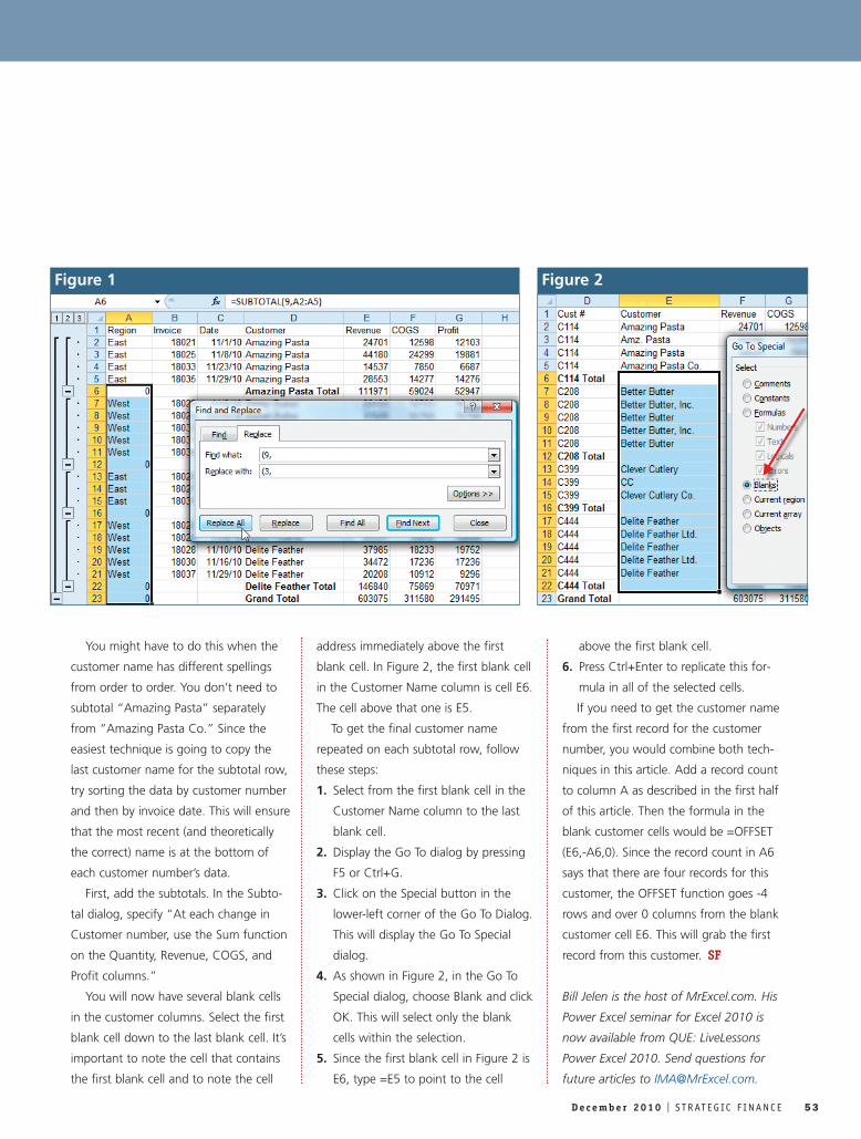
See the example in Figure 1. We began

with the subtotals of the three data fields.

Then we added a subtotal of the Region

column, resulting in a sum of 0. Now we

select column A and type Ctrl+H to dis-

play the Find and Replace dialog. As the

figure shows, we want to change every

occurrence of “(9,” to “(3,”. Once we

click Replace All, it will edit every subtotal

formula in column A to show a count

instead of a sum. The end result will be

both a sum and count total on one row.

Showing a Text Valueon the Subtotal RowsSometimes you might choose to add a

subtotal at each change in customer

number, but then you’ll want to show

the customer name associated with that

customer number on the subtotal row.

52 S T R AT E G IC F I N A N C E I D e c e m b e r 2 0 1 0

TECHNOLOGY

EXCELShowing Other Data on Subtotal Rows

By Bill Jelen

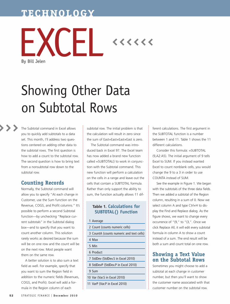
Table 1. Calculations forSUBTOTAL() Function

1 Average

2 Count (counts numeric cells)

3 CountA (counts numeric and text cells)

4 Max

5 Min

6 Product

7 StdDev (StdDev.S in Excel 2010)

8 StdDevP (StdDev.P in Excel 2010)

9 Sum

10 Var (Var.S in Excel 2010)

11 VarP (Var.P in Excel 2010)

You might have to do this when the

customer name has different spellings

from order to order. You don’t need to

subtotal “Amazing Pasta” separately

from “Amazing Pasta Co.” Since the

easiest technique is going to copy the

last customer name for the subtotal row,

try sorting the data by customer number

and then by invoice date. This will ensure

that the most recent (and theoretically

the correct) name is at the bottom of

each customer number’s data.

First, add the subtotals. In the Subto-

tal dialog, specify “At each change in

Customer number, use the Sum function

on the Quantity, Revenue, COGS, and

Profit columns.”

You will now have several blank cells

in the customer columns. Select the first

blank cell down to the last blank cell. It’s

important to note the cell that contains

the first blank cell and to note the cell

address immediately above the first

blank cell. In Figure 2, the first blank cell

in the Customer Name column is cell E6.

The cell above that one is E5.

To get the final customer name

repeated on each subtotal row, follow

these steps:

1. Select from the first blank cell in the

Customer Name column to the last

blank cell.

2. Display the Go To dialog by pressing

F5 or Ctrl+G.

3. Click on the Special button in the

lower-left corner of the Go To Dialog.

This will display the Go To Special

dialog.

4. As shown in Figure 2, in the Go To

Special dialog, choose Blank and click

OK. This will select only the blank

cells within the selection.

5. Since the first blank cell in Figure 2 is

E6, type =E5 to point to the cell

above the first blank cell.

6. Press Ctrl+Enter to replicate this for-

mula in all of the selected cells.

If you need to get the customer name

from the first record for the customer

number, you would combine both tech-

niques in this article. Add a record count

to column A as described in the first half

of this article. Then the formula in the

blank customer cells would be =OFFSET

(E6,-A6,0). Since the record count in A6

says that there are four records for this

customer, the OFFSET function goes -4

rows and over 0 columns from the blank

customer cell E6. This will grab the first

record from this customer. SF

Bill Jelen is the host of MrExcel.com. His

Power Excel seminar for Excel 2010 is

now available from QUE: LiveLessons

Power Excel 2010. Send questions for

future articles to IMA@MrExcel.com.

D e c e m b e r 2 0 1 0 I S T R AT E G IC F I N A N C E 53

Figure 1 Figure 2