HAL Id: tel-01513554https://tel.archives-ouvertes.fr/tel-01513554

Submitted on 25 Apr 2017

HAL is a multi-disciplinary open accessarchive for the deposit and dissemination of sci-entific research documents, whether they are pub-lished or not. The documents may come fromteaching and research institutions in France orabroad, or from public or private research centers.

L’archive ouverte pluridisciplinaire HAL, estdestinée au dépôt et à la diffusion de documentsscientifiques de niveau recherche, publiés ou non,émanant des établissements d’enseignement et derecherche français ou étrangers, des laboratoirespublics ou privés.

Test et apports d’outils de phénotypage racinairesdirects (imagerie des racines) et indirects (méthode

électrique capacitive) pour une utilisation en sélectionvariétale au champ : application au blé

François Postic

To cite this version:François Postic. Test et apports d’outils de phénotypage racinaires directs (imagerie des racines)et indirects (méthode électrique capacitive) pour une utilisation en sélection variétale au champ :application au blé. Autre [q-bio.OT]. Université d’Avignon, 2016. Français. <NNT : 2016AVIG0680>.<tel-01513554>

 

   

 

 

THÈSE 

pour obtenir le grade de Docteur de l’Université d’Avignon et des Pays de Vaucluse 

Test et apports d’outils de phénotypage racinaires directs (imagerie des racines) et indirects (méthode électrique capacitive)

pour une utilisation en sélection variétale au champ : application au blé

Présentée publiquement

par

François POSTIC

Soutenue le 13 décembre 2016, devant le jury composé de :

Dr. Alexia STOKES Directrice de recherche, INRA Rapporteur

Dr. Isabelle COUSIN Directrice de recherche, INRA Rapporteur

Pr Nicolas FLORSCH Professeur, Université Pierre et Marie Curie Examinateur

Dr. Christophe JOURDAN Chargé de recherche, CIRAD Examinateur

Dr. David GOUACHE Directeur de recherche, Terres Inovia Membre invité

Dr. Jean-Pierre COHAN Adjoint au Directeur scientifique, ARVALIS Membre invité

Dr. Liliana DI PIETRO Directrice de recherche, INRA Directrice de thèse

Dr. Claude DOUSSAN Chargé de recherche, INRA Encadrant

i

Remerciements

Je souhaite tout d’abord exprimer mes remerciements à Isabelle Cousin et Alexia Stokes

d’avoir accepté d’être rapporteurs de ce mémoire. Je remercie également Liliana Di Pietro,

Jean-Pierre Cohan, Nicolas Florsch, David Gouache et Christophe Jourdan d’avoir accepté

d’examiner cette thèse.

Mes remerciements s’adressent à Liliana Di Pietro, ma directrice de thèse, pour m’avoir

permis de réaliser cette thèse dans les meilleures conditions.

Je tiens à exprimer ensuite mes plus vifs remerciements à Claude Doussan qui m’a accueilli

dans son laboratoire et qui m’a encadré tout au long de ces années de thèse Je le remercie

particulièrement pour m’avoir toujours guidé, encouragé, prodigué de nombreux et importants

conseils et m’avoir fait profiter de ses vastes connaissances, tout en me laissant une grande

liberté d’action à chaque étape de cette aventure. J’ai beaucoup appris à ses côtés et je lui

adresse toute ma reconnaissance.

Je remercie grandement Katia Beauchêne d’ARVALIS pour la confiance qu’elle m’a

accordée, pour son pragmatisme et son appui dans la mise en œuvre des campagnes d’essais,

pour ses conseils avisés, pour sa disponibilité et pour s’être toujours intéressée à l’avancée de

mes travaux.

L’équipe technique Arvalis de Gréoux-les-Bains, Magali Camous, Olivier Moulin, Guillaume

Meloux et Stéphane Jezequel, pour leur inestimable expérience dans la conduite des essais

agronomiques.

Je remercie Xavier Le Bris et Baptiste Soenen d’ARVALIS pour avoir partagé leur savoir en

agronomie et ainsi contribué à l’exploitation des résultats de la campagne de mesures

racinaires au champ.

ii

Je tiens à remercier chaleureusement Arnaud Chapelet, technicien à l’UMR EMMAH, pour

son indispensable aide lors de toutes les campagnes expérimentales au champ, et ses

nombreuses heures passées à collecter, laver et trier des racines.

Je remercie les stagiaires avec qui j’ai eu la chance de travailler. Merci à Hannah Kuttler pour

les innombrables heures qu’elle a passées à effectuer les tracés de racines vues au

minirhizotron. Merci à Randa Ben Youssef et Arthur Gierczak pour leurs résultats

d’expérimentations qui ont contribué aux chapitres 1 et 3 de cette thèse.

Je remercie Phillipe Hinsinger et Ran Erel, de l’INRA Montpellier, UMR Eco&Sols, pour

m’avoir permis de d’utiliser leur campagne de mesures sur des plants de maïs et pour leurs

contributions au troisième chapitre de cette thèse.

Je tiens aussi à mentionner le plaisir que j'ai eu à travailler au sein de l’UMR EMMAH, et je

remercie ici ses membres et ex-membres que j’ai côtoyés quotidiennement durant ces années :

Mohammed Al-Khassem, Régis Marcel-Auda, Éric Avayan, Carine Baudet, Annette Bérard,

Bernard Bes, Nicolas Beudez, Elodie Canchon, Line Capowiez, Simon Carrière, Konstantinos

Chalikakis, Lucie Dal Soglio, Micheline Debroux, Guillaume Girardin, Alizée Lehoux, Anne-

Sophie Lissy, Mounia Mahkoul, Éric Michel, Nathalie Moitrier, Nicolas Moitrier, René

Pallut, Stéphane Ruy, Stéphane Sammartino, Vincent Tesson, Bernadette Thomas, Frank

Tison, Romain Van Den Bogaert.

Une pensée pour Amélie et Bastien, les stagiaires de l’année 2016, pour les bons moments

passés ;

Enfin je tiens à exprimer toute ma gratitude à ma famille qui m’a soutenu sans faille, en toute

occasion.

   

iii

Résumé

Pour soutenir la demande en denrées alimentaires d’une population mondiale croissante, les rendements des productions en céréales, notamment du blé, doivent être améliorés par sélection végétale. À cause du changement climatique et de l’épuisement des ressources fossiles, les systèmes racinaires des futures variétés de blé devront être adaptés aux épisodes de sécheresse et aux sols peu fertiles. Il est donc crucial de développer des outils de mesure de traits racinaires au champ répondant aux exigences de la sélection variétale. Ainsi, la pertinence des minirhizotrons et de l’impédance électrique des plantes a été évaluée en essai agronomique sur des variétés de blé, conçu pour obtenir un panel varié d’enracinement.

Nous avons montré que les minirhizotrons fournissent une quantification dynamique et pertinente de la longueur de racines profondes, qui jouent rôle majeur dans les rendements obtenus en conditions pluviales. Malgré une sous-estimation de la partie superficielle des systèmes racinaires, la conversion volumétrique des données issues des minirhizotrons basée sur une profondeur de champ, et à l’aide de prélèvements pour les horizons de surface, a permis une estimation du ratio de masse racinaire sur masse aérienne.

À travers une étude méthodologique en laboratoire, nous avons déterminé le montage optimal de mesure d’impédance électrique sur des plants de blé. Son application au champ montre que la qualité de l’estimation diminue au cours de la croissance et dépend de l’humidité du sol. Nous avons montré que l’impédance des plants de blé est décrite par un modèle de condensateur plan, les tissus végétaux formant un diélectrique imparfait. Ainsi, la réactance est un prédicteur de la masse racinaire, uniquement dans les couches superficielles et sèches du sol.

Mots clés : biomasse racinaire, triticum spp, blé, minirhizotron, impédance, mesures au champ

Ensuring the food supply of an increasing world population could be achieved by improving crop yields through plant breeding. Due to the climate change and the rarefaction of fossil resources, the root systems of the future wheat cultivars should be adapted to low soil moisture and low soil fertility. Developing tools for in situ root traits measurements fulfilling the high throughput requirement of modern breeding is crucial. For this purpose, an agronomic trial was conducted on wheat cultivars to evaluate the relevance of minirhizotrons and plant electrical impedance on assessing varied rooting architecture.

We showed that minirhizotrons provide dynamic and relevant quantifications of deep root lengths, which was a key factor in crop yield under rainfed conditions. In spite of underestimated lengths in the shallow part of the root systems, a volumetric conversion of minirhizotron data using a depth-of-field criterion, coupled with auger sampling for surface layers, allowed fairly estimation root to shoot ratio at different growth stages.

We determined the optimal setup of plant impedance measurements by a methodological study performed under laboratory conditions. The application of this optimal setup to an in situ survey showed that the quality of the predictions decreased at later growth stages and under low soil wetness. The plant impedance was described by an imperfect parallel-plate capacitor mode, where plant tissues acted as the separating medium. Consequently, electrical reactance is a root biomass sensor, but only in surface soil layers at low water content.

Keywords: root biomass, wheat, triticum spp, minirhizotron, electrical impedance, field measurement.

iv

v

Abréviations

DOF – Profondeur de champ, cm

GY – Rendement en grains, t.ha-1

RDM – Masse racinaire sèche totale (obtenue avec tarière et minirhizotron), t.ha-1

RLD – Densité de longueur racinaire, mm.cm-3

RLSD – Densité surfacique de longueur racinaire, mm.cm-2

R:S – Ratio de masse racinaire /masse aérienne, Sans dimension

SDM – Masse des parties aériennes, t.ha-1

SRL – Longueur spécifique racinaire m.g-1

TRLSD – Densité surfacique de longueur racinaire totale, mm.cm-2

i – Unité imaginaire, Sans dimension

A – Aire de superposition d’un condensateur, square meters, m²

C –Capacité parallèle, F

G – Conductance, S

L – Distance de séparation des plaques d’un condensateur, m

Rp –Résistance en parallèle, Ω

S – Section d’une racine, m²

X – Réactance, Ω

Y – Admittance, S

ε* – Permittivité complexe, F.m-1

ε’ – Composante réelle de la permittivité, F.m-1

ε’’ – Composante imaginaire de la permittivité, F.m-1

ω – Fréquence angulaire, rad.s-1

ω0 – Fréquence de coupure, rad.s-1

σ – Conductivité électrique, S.m-1

τ – Temps de relaxation, s 

vi

vii

Table des matières Introduction

1. Cadre général ................................................................................................................................... 2

2. Les défis à venir de l’agriculture ..................................................................................................... 4

1.1. Assurer la sécurité alimentaire mondiale d’une population croissante ........................................ 4

1.2. Perspectives climatiques ............................................................................................................... 6

1.3. Occurrence des évènements extrêmes .......................................................................................... 9

2. Caractères de sélections du blé moderne et futur .............................................................................. 10

2.1. La révolution verte ..................................................................................................................... 10

2.2. Traits liés à la révolution verte ................................................................................................... 12

2.2.1. Nanisme ................................................................................................................ 12

2.2.2. Changements phénologiques ................................................................................... 12

2.2.3. Adaptation à l’apport d’azote .................................................................................. 13

2.2.4. Tolérance aux stress hydriques ................................................................................ 14

2.2.5. Changements dans la diversité génétique ................................................................. 14

2.3. Les traits racinaires adaptés aux futures conditions climatiques ................................................ 16

2.3.1. Contexte ................................................................................................................ 16

2.3.2. Généralités sur la croissance racinaire ..................................................................... 17

2.3.3. Traits architecturaux d’intérêts dans les grandes cultures .......................................... 20

2.3.4. Les traits morphologiques et anatomiques des racines............................................... 22

3. Méthodes de mesures des systèmes racinaires .................................................................................. 24

3.1. Échelle d’observation pratiquée ................................................................................................. 24

3.2. Méthodes utilisées en milieux contrôlés..................................................................................... 24

3.2.1. Aperçu global ........................................................................................................ 24

3.2.2. Contraintes et limites des études en milieux contrôlés ............................................... 25

3.3. Méthodes applicables au champ ................................................................................................. 26

3.3.1. Inadaptation des méthodes destructives aux exigences du phénotypage ...................... 26

3.3.2. Méthodes non destructives d’observation directe ...................................................... 27

3.3.3. Méthodes non destructives de caractérisation indirectes ............................................ 29

4. Bases sur les techniques de mesures des racines employées dans cette thèse ................................... 31

4.1. Les minirhizotrons ...................................................................................................................... 31

4.1.1. Tubes d'observation ............................................................................................... 32

4.1.2. Systèmes de capture d'images des racines ................................................................ 35

viii

4.1.3. Données issues des minirhizotrons .......................................................................... 36

4.2. Mesures indirectes des systèmes racinaires par méthode électrique .......................................... 40

4.2.1. Propriétés électriques des tissus biologiques ............................................................ 40

4.2.2. Application de la mesure de l’impédance aux systèmes racinaires ............................. 44

4.2.3. Implication pour les programmes de sélection variétale ............................................ 50

Objectifs et résultats

Objectifs de la thèse ....................................................................................................... 53

Chapitre 1 : Analyse comparative des méthodes électriques pour l'estimation rapide de la biomasse racinaire ........................................................................................................... 55

Chapitre 2 : Impact des systèmes racinaires de différentes variétés de blé en conditions multi-stressantes, mis en évidence à l’aide de minirhizotrons à scanner ........................................ 69

Chapitre 3 : Un modèle étendu de l’impédance des plantes : détection in situ des racines . 117

Conclusions ........................................................................................................................... 161

Annexes ................................................................................................................................. 175

Références ............................................................................................................................. 189

 

1

Introduction

Introduction

2

1. Cadre général

La population mondiale pourrait atteindre 9 milliards d’habitants en 2050, augmentant ainsi la

pression sur les ressources alimentaires. Il est estimé qu’en 2050, la demande en blé,

actuellement la troisième céréale la plus produite à l’échelle mondiale, pourrait subir une

hausse de 39,7 % par rapport au niveau de consommation 2005–2007 (Alexandratos and

Bruinsma, 2012). Dans le même temps, la hausse des surfaces cultivables sera très faible

(1,35 %) (Alexandratos and Bruinsma, 2012), impliquant que le gain de production sera

réalisé à travers une amélioration végétale. Par ailleurs, depuis les années 2000, les

rendements du blé semblent stagner dans plusieurs régions du monde, notamment en Europe

(Brisson et al., 2010). Le changement climatique pourrait en être la cause (Brisson et al.,

2010), et les prévisions sur le futur climat de la zone Europe indiquent une forte variabilité

des précipitations (Salzmann, 2016) et une augmentation des épisodes de sécheresse, principal

facteur de stress et de perte de rendement, rendant les ressources en eau moins disponibles

pour les cultures. De plus, la raréfaction des ressources fossiles et minérales, à partir

desquelles sont produits les engrais, pourrait contraindre l’utilisation des fertilisants à moyen

terme.

Ainsi la sélection variétale doit s’attacher à améliorer l’efficacité des plants de blé à la capture

de l’eau et des nutriments présents dans le sol. Le système racinaire étant l’organe qui assure

cette fonction, l’amélioration des rendements des futures variétés pourrait s’appuyer sur une

sélection de systèmes racinaires aux traits adaptés aux futures conditions agroclimatiques.

Différents traits racinaires sont adaptés à la résistance à la sécheresse, tel un enracinement

profond pour extraire l’humidité des couches profondes du sol en période de sécheresse

Introduction

3

(Manschadi et al., 2006), ou une vigueur racinaire précoce (Bertholdsson and Brantestam,

2009).

Toutefois, à cause de sa nature souterraine, le système racinaire n’a, qu’à de très rares

occasions, fait l’objet de programmes de sélection. En effet, l’amélioration génétique du

milieu du XXème siècle (la Révolution Verte) est basée sur la sélection de traits aériens, et

depuis cette dernière décennie, de nombreux outils de phénotypages ont été conçus pour leur

mesure à haut-débit, que ce soit en serre (Fiorani and Schurr, 2013) ou au champ (Comar et

al., 2012). Les techniques d’imagerie des systèmes racinaires sont actuellement appliquées

aux serres automatisées (Jeudy et al., 2016), permettant d’atteindre les exigences de nombre

de plantes mesurées chaque jour. Cependant, les mesures au champ semblent incontournables,

car les traits racinaires obtenus aux stades végétatifs sont difficilement reproductibles à des

stades plus avancés (Watt et al., 2013). Utiliser alors des méthodes de mesure destructives

(Trachsel et al., 2011) ne serait pas adapté aux exigences de la sélection, car cela impliquerait

une utilisation intense de main-d’œuvre et une multiplication de la superficie des essais. Ces

deux difficultés sont d’autant plus présentes lorsqu’il s’agit de mesurer des dynamiques

d’enracinement, impliquant une multiplicité de dates d’échantillonnage.

À l’instar des techniques d’imagerie utilisées pour la caractérisation des traits aériens, il est

nécessaire de développer des techniques de mesures racinaires adaptées au champ, qui

devront être caractérisées par leur aspect non destructif, non invasif et rapide.

 

 

Introduction

4

2. Les défis à venir de l’agriculture

1.1. Assurer la sécurité alimentaire mondiale d’une population

croissante

Si la croissance démographique annuelle est en train de ralentir actuellement (de 1,28 % en

2000 à 1,13 % en 2015) et pour le futur, avec des prévisions en 2050 aux alentours de 0,52 %

(United Nations, Department of Economic and Social Affairs, Population Division, 2015), il

n’en reste pas moins que la population mondiale pourrait atteindre 9,3 milliards d’êtres

humains d’ici 2050, représentant ainsi un accroissement d’un tiers de la population actuelle

(7,35 milliards en 2015).

Dans le même temps, la demande mondiale en production agricole augmentera

nécessairement, représentant une hausse de 39,7 % de la production de céréales en 2050, par

rapport à la production de 2005–2007, ce qui revient à une croissance annuelle de 0,83 % sur

40 ans (Alexandratos and Bruinsma, 2012). En ce qui concerne la production agricole totale,

la hausse pourrait être plus élevée, de l’ordre de 60% (Alexandratos and Bruinsma, 2012), en

tenant compte des changements de régimes alimentaires associés à la hausse du pouvoir

économique des habitants des pays en voie de développement. Il est estimé que la demande en

produit carnés sera plus importante de 76% en 2050 (Alexandratos and Bruinsma, 2012),

induisant ainsi une hausse de la production de céréales fourragères.

De ce fait, l’équilibre entre demande et production de denrées alimentaires pourrait être plus

précaire. Un pourcentage élevé de cette demande doit être satisfait par les principales cultures

de base, le blé (Triticum aestivum L.), le riz (Oryza sativa L.), le maïs (Zea mays L.), et l'orge

(Hordeum vulgare L.). L’augmentation de la production a deux sources : l’augmentation des

Introduction

5

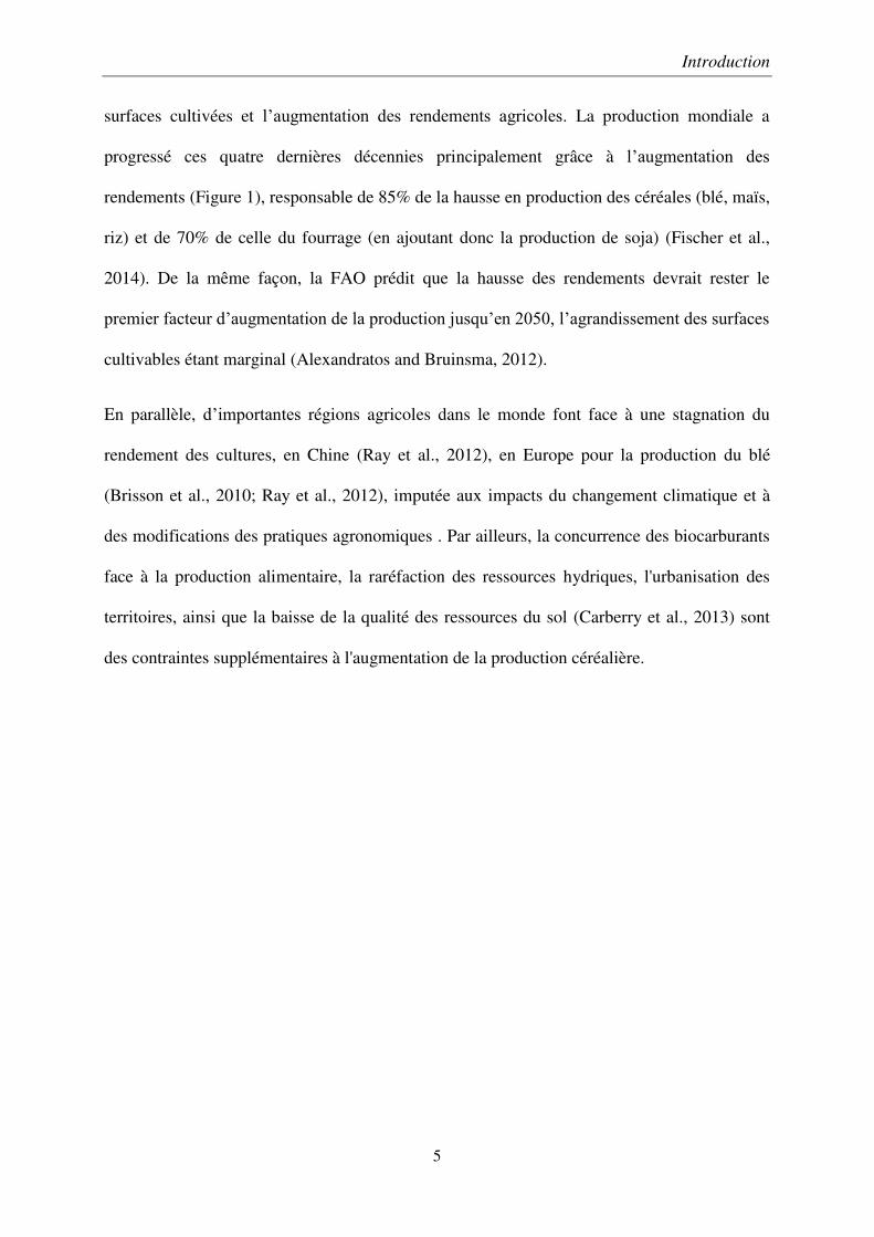
surfaces cultivées et l’augmentation des rendements agricoles. La production mondiale a

progressé ces quatre dernières décennies principalement grâce à l’augmentation des

rendements (Figure 1), responsable de 85% de la hausse en production des céréales (blé, maïs,

riz) et de 70% de celle du fourrage (en ajoutant donc la production de soja) (Fischer et al.,

2014). De la même façon, la FAO prédit que la hausse des rendements devrait rester le

premier facteur d’augmentation de la production jusqu’en 2050, l’agrandissement des surfaces

cultivables étant marginal (Alexandratos and Bruinsma, 2012).

En parallèle, d’importantes régions agricoles dans le monde font face à une stagnation du

rendement des cultures, en Chine (Ray et al., 2012), en Europe pour la production du blé

(Brisson et al., 2010; Ray et al., 2012), imputée aux impacts du changement climatique et à

des modifications des pratiques agronomiques . Par ailleurs, la concurrence des biocarburants

face à la production alimentaire, la raréfaction des ressources hydriques, l'urbanisation des

territoires, ainsi que la baisse de la qualité des ressources du sol (Carberry et al., 2013) sont

des contraintes supplémentaires à l'augmentation de la production céréalière.

Introduction

6

Figure 1. Rendement moyen des cultures de blé à l’échelle mondiale sur la période 1960-

2014 (Données FAO 2016). La période 1960–1990 est caractérisée par une progression

constante des rendements (courbe rouge), un ’infléchissement des rendements apparait à partir

des années 1990 (courbe bleue).

1.2. Perspectives climatiques

 

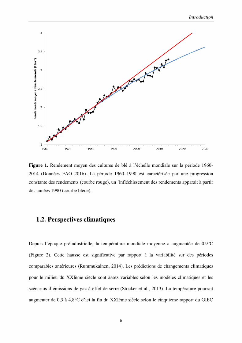
Depuis l’époque préindustrielle, la température mondiale moyenne a augmentée de 0.9°C

(Figure 2). Cette hausse est significative par rapport à la variabilité sur des périodes

comparables antérieures (Rummukainen, 2014). Les prédictions de changements climatiques

pour le milieu du XXIème siècle sont assez variables selon les modèles climatiques et les

scénarios d’émissions de gaz à effet de serre (Stocker et al., 2013). La température pourrait

augmenter de 0,3 à 4,8°C d’ici la fin du XXIème siècle selon le cinquième rapport du GIEC

Introduction

7

(Stocker et al., 2013). D’après des simulations climatiques, une augmentation des

précipitations mondiales accompagnera ce réchauffement climatique. Ces simulations

indiquent une hausse d’environ 1% pour chaque hausse de 1°C de la température moyenne

mondiale (Rummukainen, 2014).

Figure 2. Variation de la température annuelle moyenne sur la période 1901–2012 d’après le

GIEC 2013, extrait de Stocker et al (2013)

Introduction

8

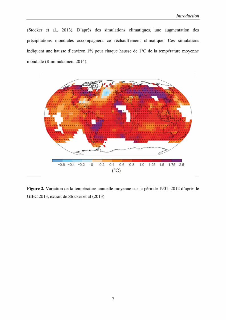
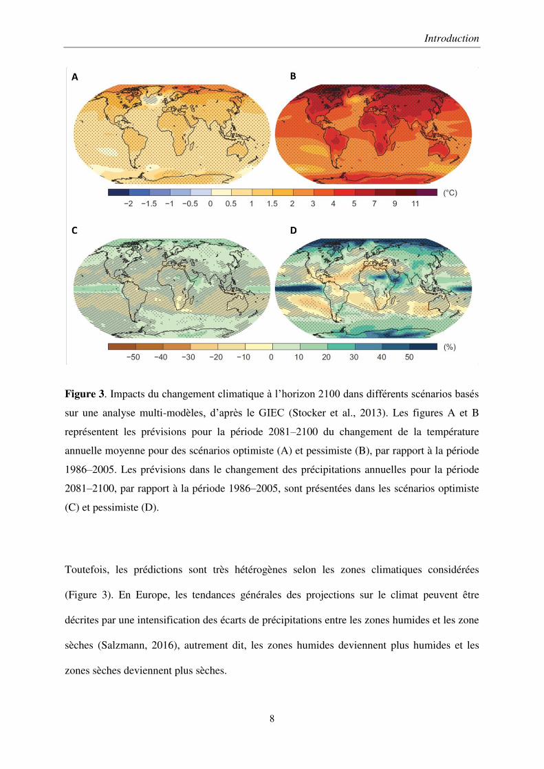
Figure 3. Impacts du changement climatique à l’horizon 2100 dans différents scénarios basés

sur une analyse multi-modèles, d’après le GIEC (Stocker et al., 2013). Les figures A et B

représentent les prévisions pour la période 2081–2100 du changement de la température

annuelle moyenne pour des scénarios optimiste (A) et pessimiste (B), par rapport à la période

1986–2005. Les prévisions dans le changement des précipitations annuelles pour la période

2081–2100, par rapport à la période 1986–2005, sont présentées dans les scénarios optimiste

(C) et pessimiste (D).

Toutefois, les prédictions sont très hétérogènes selon les zones climatiques considérées

(Figure 3). En Europe, les tendances générales des projections sur le climat peuvent être

décrites par une intensification des écarts de précipitations entre les zones humides et les zone

sèches (Salzmann, 2016), autrement dit, les zones humides deviennent plus humides et les

zones sèches deviennent plus sèches.

Introduction

9

Par ailleurs, l'intensité, la durée et la fréquence des vagues de chaleur sont fortement

susceptibles d'augmenter (Coumou and Rahmstorf, 2012). La fréquence des évènements

climatiques extrêmes est le résultat de changements concernant les moyennes des variables

climatiques, de leur variance, ou d’une modification de la distribution statistique de ces

variables (Stocker et al., 2013). Les études qui ne considèrent que les changements des

moyennes des variables climatiques pourraient conclure de façon erronée sur l’incidence des

évènements extrêmes (Rummukainen, 2014).

1.3. Occurrence des évènements extrêmes

Le changement climatique provoquant une variabilité accrue des conditions météorologiques,

ainsi qu’une recrudescence des phénomènes climatiques extrêmes, impacte négativement la

production alimentaire et, par conséquent, la sécurité alimentaire (Coumou and Rahmstorf,

2012). L’augmentation de la fréquence des phénomènes extrêmes tels que les vagues de

chaleur et les sécheresses prolongées est déjà observable (Christidis et al., 2014), entrainant

des impacts négatifs majeurs sur la production agricole dans de nombreuses régions du

monde. Ce fut le cas en 2007, 2010 et 2012 avec une occurrence simultanée de phénomènes

météorologiques défavorables dans les régions agricoles importantes (Lobell and Gourdji,

2012). Les projections sur le climat futur prédisent une fréquence significativement plus

élevée d'années très défavorables pour la production agricole, provoquant des retombées

économiques désastreuses dans de nombreuses régions agricoles (Stocker et al., 2013). 

Afin de faire face aux défis du changement climatique futur, caractérisé par l'augmentation

des phénomènes météorologiques extrêmes, il est primordial d’adapter les systèmes de

production agricole (Trnka et al., 2014). En outre, les incertitudes sur les projections des

Introduction

10

changements climatiques posent des défis particuliers aux obtenteurs variétaux et aux

scientifiques du domaine de l’amélioration variétale (Semenov et al., 2014).

2. Caractères de sélections du blé moderne et futur

2.1. La révolution verte

La révolution verte est le processus qui décrit l’introduction de la génétique dans

l’amélioration variétale avec des variétés à haut rendement, couplée à la mécanisation et à

l’utilisation intensive d’intrants (eau, fertilisants, produits phytosanitaires). Elle a commencé

dans les années 60 avec Norman Borlaug qui a développé des cultivars de blé tendre (Triticum

aestivum) aux tiges plus courtes, à haut rendement. La création au Mexique du Centro

internacional de mejoramiento de maiz y trigo (CIMMYT ou centre international

d'amélioration du maïs et du blé), grâce aux efforts de Norman Borlaug (prix Nobel de la Paix

en 1970), a permis aux sélectionneurs de développer des blés semi-nains et résistants aux

maladies caractéristiques des zones humides telles la septoriose et la fusariose. Ces cultivars

adaptés aux zones humides ont rapidement été diffusés dans l’Asie du Sud pour faire face à

l’insécurité alimentaire de cette époque.

Ces changements de hauteur des plantes, accompagnés par une meilleure résistance aux

maladies, ont participé à l’augmentation des rendements ainsi qu’à leur stabilité. L'impact

global du programme de sélection du blé de CIMMYT a été important et bien documenté

(Lopes et al., 2012). À cet égard, la progression annuelle des rendements fournit un moyen

pour évaluer le succès d'un programme de sélection végétale.

Comme on peut l’observer sur la Figure 1, les rendements de blé dans le monde entier ont

augmenté de manière relativement linéaire, bien que cette croissance se soit tassée dans les

Introduction

11

quinze dernières années. Sur la période 1990–2014, les rendements du blé ont alors enregistré

un hausse de 1,38% par an en moyenne (Food and Agriculture Organization, 2016), alors que

sur la période 1960–2014, et le rendement moyen du blé au niveau mondial a augmenté au

rythme d’environ 2,25% par an.

Bien que la base génétique de la révolution verte du blé ait d'abord été « simple » et impliqué

l'introduction dans le génome du blé de quelques gènes avec des effets majeurs — sur la

hauteur de la plante et l'élimination de la réponse de la photopériode pour la culture en zone

équatoriale — , les sélectionneurs ont maintenu des progrès dans l'amélioration génétique du

rendement du blé par la manipulation des systèmes de gènes de plus en plus complexes.

La sélection variétale internationale du blé réalisée par le CIMMYT peut être divisée en

quatre périodes d'amélioration de 1951 à nos jours (Ortiz et al., 2008) :

- de 1951 à 1962, introduction chez les agriculteurs de cultivars avec une meilleure

résistance de la tige face à la verse, et des feuilles face à la rouille brune du blé

(Puccinia triticina.) ;

- de 1962 à 1975, introduction chez les agriculteurs de cultivars semi-nains ;

- de 1975 aux années 1990, amélioration du potentiel de rendement, de la résistance

aux maladies (notamment la rouille dont la résistance des souches s’est accrue) et

amélioration de la qualité industrielle (taux de protéines) de cultivars semi-nains ;

- enfin, depuis les années 1990, amélioration de la tolérance aux stress abiotiques,

utilisation de cultivars de blé hybrides et synthétiques, et amélioration de la qualité du

grain.

Introduction

12

2.2. Traits liés à la révolution verte

2.2.1. Nanisme

Les cultivars semi-nains de blé apparus dans les années 70 sont caractérisés par leurs tiges

plus courtes (Trethowan et al., 2002) que celles des cultivars traditionnels. Ainsi ils sont plus

tolérants à la verse et possèdent un potentiel de rendement plus élevé que les cultivars

traditionnels du fait qu’une forte proportion de leur biomasse soit consacrée aux grains (et non

à la tige). Ce phénotype semi-nain est contrôlé par deux gènes d’insensibilité à l’acide

gibbérellique, les gènes Rht1 et Rht2, découverts par Borlaug (1968). La présence d’un seul

de ces deux gènes produit un cultivar semi-nain, alors que leur présence simultanée produit un

cultivar double nain. La courte stature des cultivars double nains n’est appropriée qu’aux

environnements les plus productifs dans lesquels l'eau et l'engrais ne sont pas limitants.

2.2.2. Changements phénologiques

L’essentiel des traits associés à l’augmentation des rendements concernent les parties

aériennes. Le rendement des cultivars semi-nains continue d’augmenter de 1% par an avec les

progrès génétiques (Ortiz et al., 2008). Au-delà du rendement potentiel, la stabilité du

rendement face aux différentes conditions environnementales est une caractéristique

agronomique importante. Cependant, l’adaptation des cultivars à des environnements

spécifiques n’apparait pas être une solution efficace, à cause de la variabilité des

précipitations annuelles dans la plupart des régions de cultures (Ortiz et al., 2008).

De nombreuses études montrent que l’augmentation des potentiels de rendements est associée

à une augmentation de la biomasse totale, du nombre de grains par mètre carré, du rapport

grain sur paille et à une hausse de l’efficacité à intercepter le rayonnement

photosynthétiquement actif (Sayre et al., 1997). Chez les cultivars les plus récents, il semble

Introduction

13

que le poids des grains contribue peu à l’amélioration récente des potentiels de rendements,

l’essentiel de l’amélioration reposant sur l’efficacité d’interception du rayonnement

photosynthétiquement actif avant floraison (Shearman et al., 2005).

De même, les gènes Rht1 et Rht2 impliquent des changements plus subtils pour l’obtention de

rendements élevés, grâce à une adaptation à de fortes densités de semis. En effet, il apparait

que les cultivars semi-nains sur la base des gènes Rht1 et Rht2 sont plus adaptés à la culture à

des densités de plantes élevées que des cultivars traditionnels (Reynolds et al., 1994).

Parmi les autres modifications physiologiques, une comparaison des cultivars de blé publiée

entre 1962 et 1988 au Mexique a montré une augmentation de 27% de rendement associé à

une augmentation de 63% de la conductance stomatique, une augmentation de 23% du taux de

photosynthèse maximale et une baisse de 6°C de la température de la canopée (Fischer et al.,

1998). Une température de canopée plus froide mesurées chez certains cultivars pourrait être

liée à leur capacité à puiser l’eau des couches profondes du sol, dans les environnements

sujets à la sécheresse (Lopes and Reynolds, 2010).

2.2.3. Adaptation à l’apport d’azote

La Révolution verte est critiquée sur l’efficacité des cultivars dans les environnements où

l’azote est une ressource limitante. En effet, les cultivars développés sont issus de sélections

destinées à produire des génotypes obtenant des rendements élevés en conditions potentielles,

autrement dit sans limitation de l’apport d’eau et d’azote. En conséquence, les cultivars

obtenus pourraient ne pas être adaptés aux conditions limitantes, et l’efficience de l’utilisation

de l’azote — c’est-à-dire la quantité de biomasse produite par rapport à la quantité d’azote

présent dans la plante — pourrait être plus faible dans les cultivars modernes. La tendance

semble cependant être inverse. Sur une sélection de cultivars enregistrés au catalogue français

Introduction

14

entre 1940 et 1995, l’efficience de l’utilisation de l’azote est améliorée avec la date de

d’entrée au catalogue (Le Gouis et al., 2000), que ce soit en conditions limitantes en azote ou

optimales, hormis pour trois variétés sur les vingt testées. Le même constat apparait sur les

cultivars diffusés au Mexique entre 1950 et 1985 (Ortiz-Monasterio et al., 1997). L’efficience

de l’utilisation de l’azote est elle-même une caractéristique composite, et il semble que ce soit

le taux d’absorption qui contribue le plus à l’efficacité des cultivars en situation d’azote

limitant (Ortiz-Monasterio et al., 1997).

2.2.4. Tolérance aux stress hydriques

Bien que la base génétique de la tolérance à la sécheresse du blé soit complexe et mal

comprise, l'analyse historique des rendements de blé du réseau d'essai international du

CIMMYT montre clairement que l'adaptation au déficit hydrique des variétés s'améliore avec

le temps (Trethowan et al., 2002). L'architecture des racines est un élément de cette

amélioration de l'utilisation de l'eau des cultures; par exemple, des racines plus longues sont

en mesure d'accéder à l'eau plus profondément dans le profil du sol (Araus et al., 2002).

2.2.5. Changements dans la diversité génétique

Les premières années de la révolution verte sont marquées par une diminution de la diversité

génétique à cause du faible nombre de cultivars semi-nains différents, cultivés sur de vastes

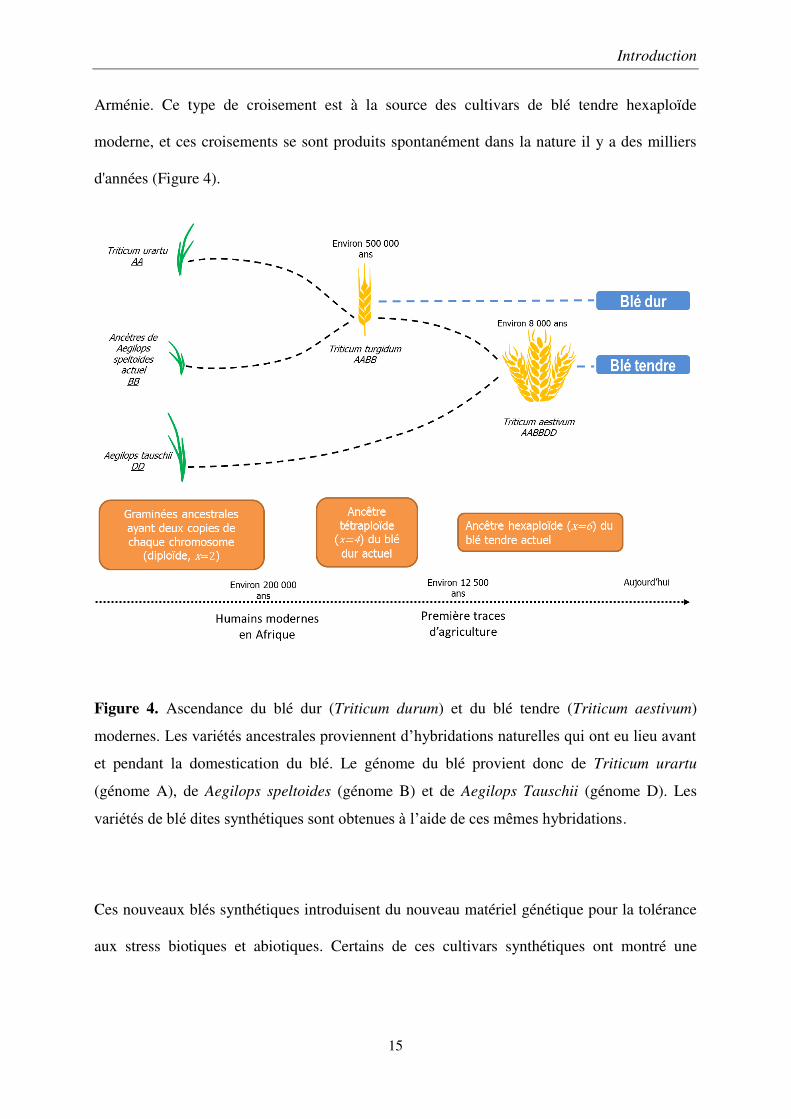
zones (Pretty, 1995). Néanmoins, une source récente de diversité génétique a été introduite

avec les cultivars de blé dits synthétiques. Ces blés synthétiques sont développés en croisant

des variétés de blé dur moderne (Triticum turgidum) avec Aegilops tauschii, l’espèce

identifiée comme le donneur probable du génome D du blé (la nomenclature du génome du

blé est précisée sur la Figure 4), originaire du Moyen-Orient, notamment dans l’actuelle

Introduction

15

Arménie. Ce type de croisement est à la source des cultivars de blé tendre hexaploïde

moderne, et ces croisements se sont produits spontanément dans la nature il y a des milliers

d'années (Figure 4).

Figure 4. Ascendance du blé dur (Triticum durum) et du blé tendre (Triticum aestivum)

modernes. Les variétés ancestrales proviennent d’hybridations naturelles qui ont eu lieu avant

et pendant la domestication du blé. Le génome du blé provient donc de Triticum urartu

(génome A), de Aegilops speltoides (génome B) et de Aegilops Tauschii (génome D). Les

variétés de blé dites synthétiques sont obtenues à l’aide de ces mêmes hybridations.

Ces nouveaux blés synthétiques introduisent du nouveau matériel génétique pour la tolérance

aux stress biotiques et abiotiques. Certains de ces cultivars synthétiques ont montré une

Introduction

16

amélioration des rendements en cas de sécheresse et se sont révélés être de nouvelles sources

utiles pour la résistance aux maladies (van Ginkel and Ogbonnaya, 2007).

2.3. Les traits racinaires adaptés aux futures conditions

climatiques

2.3.1. Contexte

Le changement climatique pourrait intensifier les conditions défavorables pour la croissance

des plantes cultivées telles que la diminution des ressources en eau, l’augmentation de la

salinité des sols et l’appauvrissement en nutriments des sols. Les traits racinaires qui

permettent une meilleure utilisation des ressources souterraines devraient donc être d’une

importance cruciale afin de préserver, voire d’augmenter, les rendements futurs. Au-delà

d’assurer la fonction d’ancrage, le système racinaire détermine la capacité d’une plante à

absorber les nutriments et l’eau présents dans le sol et d’autres fonctions importantes dans un

environnement donné tels la production d’hormones, le stockage d’assimilats ou les

associations symbiotiques (Hodge et al., 2009). Bien que la plupart des études portant sur les

stress observent des traits architecturaux (configuration spatiale des racines), d’autres

adaptations anatomiques entrent en jeu dans l’efficacité du système racinaire (Figure 5). Les

effets sur le système racinaire de stress uniques sont nettement plus documentés que les effets

d’une combinaison de stress (Rich and Watt, 2013). Ces conditions multi-stressantes pouvant

être plus fréquentes dans l’avenir, le 2ème chapitre de cette thèse porte sur l’effet in situ de

telles combinaisons de stress.

Introduction

17

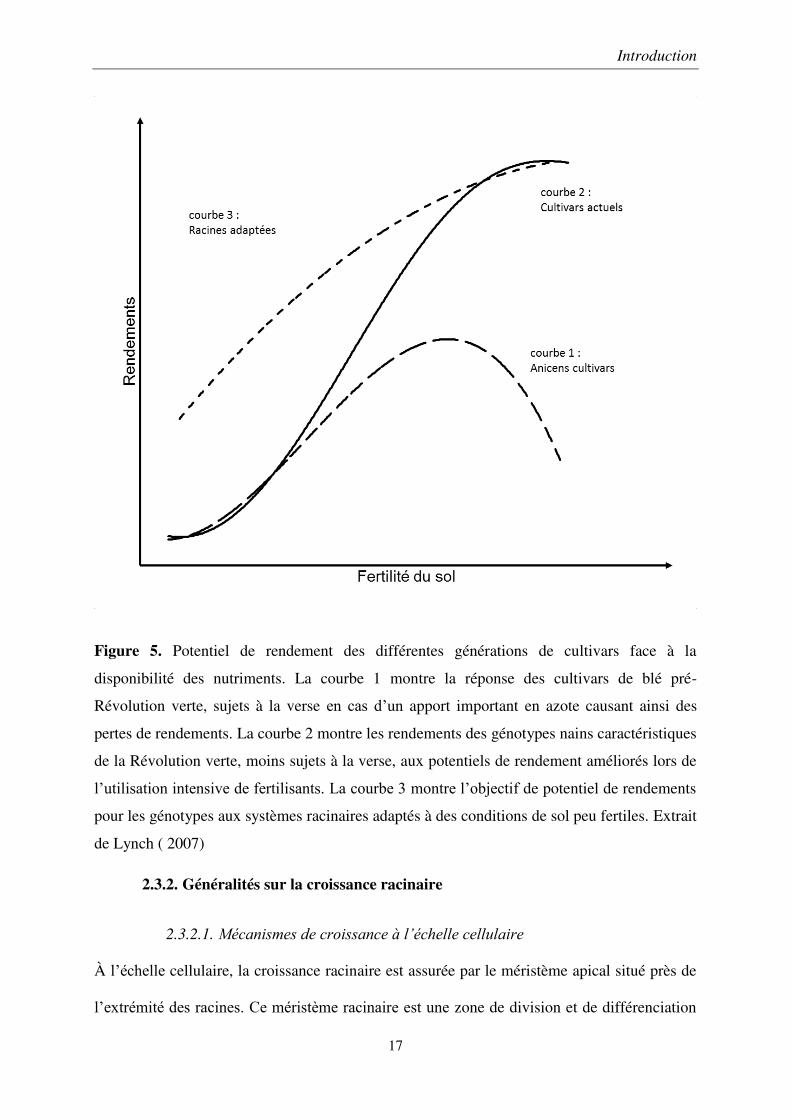
Figure 5. Potentiel de rendement des différentes générations de cultivars face à la

disponibilité des nutriments. La courbe 1 montre la réponse des cultivars de blé pré-

Révolution verte, sujets à la verse en cas d’un apport important en azote causant ainsi des

pertes de rendements. La courbe 2 montre les rendements des génotypes nains caractéristiques

de la Révolution verte, moins sujets à la verse, aux potentiels de rendement améliorés lors de

l’utilisation intensive de fertilisants. La courbe 3 montre l’objectif de potentiel de rendements

pour les génotypes aux systèmes racinaires adaptés à des conditions de sol peu fertiles. Extrait

de Lynch ( 2007)

2.3.2. Généralités sur la croissance racinaire

2.3.2.1. Mécanismes de croissance à l’échelle cellulaire

À l’échelle cellulaire, la croissance racinaire est assurée par le méristème apical situé près de

l’extrémité des racines. Ce méristème racinaire est une zone de division et de différenciation

Introduction

18

cellulaire, complexe et hétérogène en terme de population cellulaire (Webster and MacLeod,

1980). Dans cette zone apparait une première différenciation qui conduit à la formation des

cellules de la coiffe (cellules situés à l’extrémité des racines) et des cellules responsables de

l’élongation des racines (la différentiation et la spécialisation ayant lieu dans un second

temps). Cette élongation à partir du méristème est nommée croissance primaire et

l’augmentation du diamètre des racines est désignée par croissance secondaire. Bien que

généralement absente chez les monocotylédones (groupe incluant le blé), cette croissance

secondaire joue un rôle majeur chez les espèces ligneuses, en étant à l’origine de la formation

du xylème et du phloème secondaires (tissus transportant l’eau et les nutriments). À cette

échelle, plusieurs traits clés dans l’adaptation à des conditions limitantes sont déterminés tels

le diamètre et la masse linéique des racines (Fitter et al., 2002).

2.3.2.2. Plasticité à l’échelle du système racinaire

La configuration spatiale du système racinaire d’une plante au cours du temps forme

l’architecture racinaire, qui est déterminée par la croissance des différents types de racines du

système racinaire (par exemple les racines principales déterminent le volume de sol

exploitable tandis que les racines d’ordre supérieur déterminent la colonisation et

l’exploitation de ce volume). Les plantes étant immobiles, l’adaptation de leur système

racinaire est une stratégie capitale pour faire face aux variations temporelles et spatiales de la

disponibilité de l’eau et des nutriments dans le sol (Hodge et al., 2009). Pour faire face à cette

variabilité des sources de nutriments, l’initiation et l’élongation de racines secondaires (ou

latérales) est un facteur clé de l’adaptation du système racinaire (Hodge et al., 2009). Ces

racines latérales permettent à la plante d’explorer le sol et de le coloniser dans les zones riches

en nutriments. En cas de conditions limitantes en nutriments, les plantes peuvent au contraire

réduire la croissance de ces racines latérales dans les zones appauvries et maintenir une

Introduction

19

croissance des racines primaires pour explorer des zones plus profondes du sol (Deak and

Malamy, 2005). Par exemple, dans le cas du haricot (Phaseolus vulgaris L.), une faible

disponibilité des nutriments phosphatés en surface entraine une augmentation de l’élongation

au détriment de l’initiation de racines latérales (Borch et al., 1999).

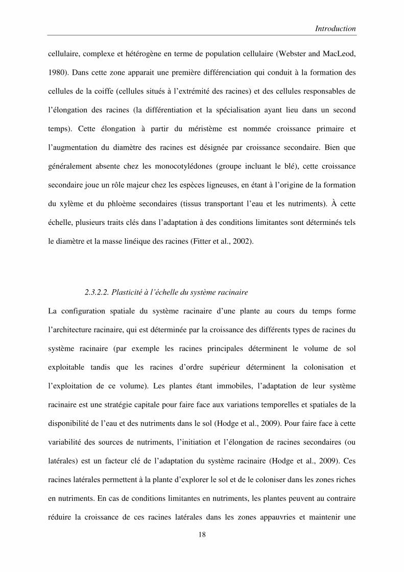
L’architecture racinaire diffère selon les espèces (Figure 6), et des variations génotypiques

chez une même espèce existent, notamment chez les céréales (Manschadi et al., 2008).

Figure 6. Exemples de la variabilité de différentes architectures racinaires classée suivant la

dominance de l’axe racinaire principal (en horizontal) et de la densité de ramification de ces

axes (en vertical), adapté de Kutschera L (1960) pour les architectures racinaires.

Introduction

20

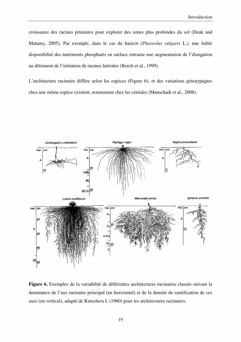
Dans le cas du blé, l’architecture racinaire est largement déterminée par l’angle de croissance

des racines séminales (radicule issue de la graine) et nodales (ou adventives), qui semble être

associé à l’efficience d’acquisition de l’eau et des nutriments phosphatés (Manschadi et al.,

2013). Les génotypes présentant des racines séminales et nodales aux angles plus verticaux

forment des systèmes compacts et profonds, alors que les génotypes présentant des racines

séminales et nodales aux angles plus horizontaux tendent à former des systèmes larges et

superficiels (Manschadi et al., 2010 — Figure 7).

Figure 7. Systèmes racinaires de plants de céréales 33 jours après leur levée. Sont présentés

des cultivars de blé SeriM82 (A) et Hartog (B), la figure C est un cultivar d’orge (Hordeum

vulgare L.) Mackay. Extrait de Manschadi et al. (2008)

2.3.3. Traits architecturaux d’intérêts dans les grandes cultures

2.3.3.1. La profondeur d’enracinement

La durée de croissance et la profondeur d’enracinement dans le sol des racines du blé est

approximativement reliée au temps nécessaire à la floraison (Gregory et al., 1978). Ainsi un

moyen d’augmenter la profondeur d’enracinement consiste à allonger le temps nécessaire

Introduction

21

pour atteindre le stade de floraison. Ainsi, un semis plus précoce augmente la profondeur

racinaire et améliore l’efficacité de l’utilisation de l’eau (Passioura and Angus, 2010).

Des variations de profondeur du système racinaire, suivant les génotypes, peuvent résulter

d’une pousse plus rapide, citée comme la vigueur racinaire (Palta and Watt, 2009), et/ou des

angles d’émissions des racines primaires plus verticaux (Manschadi et al., 2010).

En ce qui concerne la prolifération des racines latérales, il peut exister une croissance

racinaire après floraison et ses effets sur le rendement pourraient être significatifs.

D’importantes différences dans la prolifération des racines profondes après floraison ont été

observées entre différents génotypes de blé (Manschadi et al., 2006) et il a été observé que le

génotype présentant le plus fort accroissement des racines profondes après floraison a obtenu

un rendement supérieur.

2.3.3.2. L’exploration racinaire des couches superficielles

Dans la plupart des cultures céréalières, la densité de longueur racinaire en surface est forte,

dépassant les 3–5 cm.cm-3. Pour l’extraction d’eau, cette densité forte excèderait la densité

requise pour extraire l’eau disponible en surface (Passioura, 1983). Dans le cas de cultures

non-irriguées, où des déficits hydriques sont possibles en cours/fin de saison, une diminution

de la quantité (densité) de racine dans ces horizons superficiels pourrait s’avérer bénéfique

pour le blé, mais au détriment de la capture de nutriments au cours de la saison (Wasson et al.,

2012). En effet, cette profusion de racines superficielles pourrait être également

particulièrement utile pour la capture des nutriments (Zhu et al., 2005) en période humide

(début de saison), tels que les nutriments peu mobiles Zn et P, qui sont de première

importance lors du remplissage du grain.

Introduction

22

2.3.3.3. L’exploration des couches profondes

Il est estimé qu’il faut environ 1cm de racines pour extraire l’eau disponible dans 1cm3 de sol,

en considérant un temps suffisant, un bon contact racines-sol et une conductivité hydraulique

sol-racines suffisante (Passioura, 1983). À la récolte, les céréales/les cultures avec une densité

de longueur racinaire insuffisante en profondeur peuvent laisser de l’humidité inexploitée

dans les couches profondes du sol. Or, il a été montré que des quantités modestes d’eau

supplémentaires exploitées en post-floraison, en cas de déficit hydrique, conduisent à un

augmentation substantielle du rendement, de l’ordre de 60 kg/ha par mm d’eau (Kirkegaard et

al., 2007). Puisque un système plus profond va de pair avec plus d’eau accessible, une

augmentation de la longueur racinaire dans ces zones est également nécessaire pour les

exploiter au mieux.

Dans le cas du blé, sur une base de modélisation et de données de précipitation (Lilley and

Kirkegaard, 2011), il a été montré qu’une pénétration plus rapide des racines (20%) induisant

un système racinaire plus profond et couplé avec une meilleure extraction de l’eau dans le

sous-sol (20% en-dessous de 60cm), pourrait ainsi augmenter les rendements. Dans une zone

où le stock d’eau profonde se forme durant la saison de culture (le sud de l’Australie dans

l’étude), de tels systèmes racinaires pourraient produire une hausse moyenne du rendement de

0.32 t.ha-1. De même, dans une zone où le stock d’eau profonde se forme avant la saison de

culture (le nord de l’Australie), la hausse de rendement pourrait atteindre 0.44 t.ha.

2.3.4. Les traits morphologiques et anatomiques des racines

La réduction du coût métabolique de l’exploration du sol est un des traits intéressants pour

optimiser l’efficience du système racinaire. Pour réduire ce coût, une solution possible est de

réduire le diamètre des racines ou la densité des tissus. Ainsi pour chaque gramme de racine

Introduction

23

produit, le volume de sol exploré est plus important. Une réduction du diamètre des racines

peut être provoquée par une faible disponibilité en nutriments (Zhu and Lynch, 2004), mais il

existe aussi des variations génotypiques du diamètre des racines primaires et latérales

associées à de plus grandes longueurs spécifiques (SRL) des racines latérales (Zhu and Lynch,

2004).

La conductance hydraulique des racines pourrait être également un des leviers pour optimiser

la quantité d’eau extraite du sol. La conductivité hydraulique axiale (de la racine vers la tige)

est nettement plus élevée que la conductivité hydraulique radiale (du sol vers la racine)

(Rowse and Goodman, 1981). Dans le but d’améliorer la capture des intrants, et pour partie la

conductivité hydraulique radiale, augmenter la densité des poils racinaires peut être une

solution. En effet, ces poils racinaires participent à l’augmentation de la conductivité

hydraulique sol-racines en agrandissant la surface de contact entre les racines et le sol. Cela

est confirmé par l’analyse d’absorption d’eau par des jeunes plants d’orge mutants dépourvus

de poils racinaires (Segal et al., 2008). Par ailleurs, deux gènes contrôlant l’élongation des

poils racinaires ont été identifiés chez le maïs, RTH1 et RTH3, et pourraient être d’intérêt

pour l’amélioration génétique (Hochholdinger and Tuberosa, 2009).

À l’inverse, réduire la conductance axiale des racines permettrait de réduire la quantité d’eau

prélevée en début de saison, et donc de sécuriser une partie de l’eau disponible en pré-

floraison, pour une meilleure utilisation en post-floraison. Ceci a été tenté, avec un certain

succès, pour le blé en Australie en sélectionnant des variétés avec des racines séminales

présentant une conductance axiale réduite (Richards et Passioura, 1989, Passioura, 1991).

Introduction

24

3. Méthodes de mesures des systèmes racinaires

3.1. Échelle d’observation pratiquée

Bien que les détails fins de la structure des racines soient importants, notamment le rôle des

poils racinaires dans l’absorption de nutriments, le système racinaire est généralement étudié

dans son ensemble (Lynch, 1995). Cette architecture globale du système racinaire possède un

rôle important dans l’adaptation des cultures aux conditions limitantes (Fitter, 2002; Lynch,

1995), notamment aux conditions de sécheresse, qui seront d’autant plus récurrentes du fait du

réchauffement climatique. Malgré cette échelle d’observation relativement large, quantifier

rapidement un grand nombre de systèmes racinaires reste un défi.

3.2. Méthodes utilisées en milieux contrôlés

3.2.1. Aperçu global

Les méthodes en milieux contrôlés bénéficient des progrès de la robotisation et des

technologies de capteurs, à travers la mise au point de serres automatisées appelées

plateformes de phénotypage. Récemment, des plateformes à but commercial ou développées

par des acteurs du domaine public ont été déployées sous la forme de serres automatisées. Ces

plateformes sont spécifiquement conçues pour la recherche et le phénotypage haut débit sur

un panel limité d’espèces, comprenant les céréales majeures (Bock et al., 2010; De Smet et

al., 2012; Sultan, 2000). Le but de ces plateformes est de fournir tout un éventail de mesures

pour chaque plante en culture grâce à la robotique (pour les aspect logistiques) et l’analyse

d’image, tout en assurant un contrôle de l’environnement de culture (Fiorani and Schurr,

2013).

Introduction

25

Dans ces serres de phénotypage, les systèmes racinaires peuvent être imagés directement

grâce aux parois transparentes des pots ou des rhizotrons de culture. Dans ce cas, les capteurs

utilisés pour l’imagerie des parties aériennes peuvent être également utilisés pour caractériser

les systèmes racinaires dans le spectre visible/infrarouge. Les plantes sont cultivées soit sur

substrat naturel (Devienne-Barret et al., 2006), soit sur substrat artificiel (Jeudy et al., 2016)

afin d’augmenter le contraste visuel entre le système racinaire et son milieu de croissance.

Des techniques permettant d’imager/quantifier directement le système racinaire dans le sol

telles que l’imagerie par résonance magnétique (IRM) et la tomographie à rayons X,

nécessitent du matériel couteux et sont peu répandues actuellement.

Par exemple, l’IRM a permis de mesurer l’effet de la taille des pots sur le système racinaire

de plants d’orge (Poorter et al., 2012) ou la distribution racinaire de plants de maïs cultivés

avec une autre espèce dans le même pot (Rascher et al., 2011). La tomographie à rayons X

fournit des données volumétriques sur l’hétérogénéité du sol (Pierret et al., 2002; Young et

al., 2008) et sur les structures des plantes (Stuppy et al., 2003). Au-delà de la disponibilité et

du coût, les limites sont principalement liées au traitement d’image nécessaire, qui peut être

source d’une grande variabilité, par exemple dans la longueur racinaire estimée (Flavel et al.,

2012).

3.2.2. Contraintes et limites des études en milieux contrôlés

L’observation des traits des systèmes racinaires en milieux contrôlés, en pots ou en rhizotrons

2D, à des stades relativement développés, est problématique. Les systèmes racinaires

atteignent rapidement les limites du container, modifiant la croissance et le développement

que les racines auraient eu naturellement au champ. Ainsi, des traits racinaires exprimés en

milieu contrôlé à des stades jeunes ne sont pas toujours corrélés aux traits observés au champ

Introduction

26

à des stades plus âgés (Watt et al., 2013). Pour assurer des mesures sur des systèmes

racinaires plus proches de la réalité terrain, il est possible d’augmenter le volume des pots (ce

qui réduit drastiquement la faisabilité des expérimentations et des répétitions) ou d’opter pour

des mesures au champ. Dans ce cas, les systèmes racinaires peuvent se développer plus

profondément et en conditions réelles. Toutefois, ce choix possède des inconvénients

majeurs : un contrôle difficile de l’environnement climatique, du sol et de son hétérogénéité,

la difficulté d’observer le système racinaire et d’obtenir des échantillons de racines, et

finalement du volume d’échantillons nécessaires à une quantification fiable.

3.3. Méthodes applicables au champ

3.3.1. Inadaptation des méthodes destructives aux exigences du phénotypage

Les techniques de caractérisations au champ de traits des parties souterraines des plantes ne

sont pas aussi développées qu’en milieu contrôlé, en particulier dans le cadre du phénotypage

non destructif et haut-débit. Du fait de leur croissance dans le sol, milieu opaque et difficile à

investiguer, l’étude des systèmes racinaires nécessite des techniques bien spécifiques. Les

techniques classiques d’études in situ comprennent des méthodes destructives : prélèvement

d’échantillons de sol, que ce soit à l’aide de tarière ou en excavant des blocs entiers de sol

(monolithes), tranchées d’observation (verticales ou horizontales).

En condition de culture au champ, la sélection végétale nécessite la caractérisation de traits

d’intérêt des plantes avec comme condition de caractériser un grand nombre de plantes dans

un court laps de temps. Dans cet objectif, un protocole de mesures destructives basé sur

l’excavation de la partie proximale du système racinaire a été mis au point pour les cultures de

maïs (Trachsel et al., 2011). Dénommé Shovelomics, ce protocole de mesure reposait

initialement sur des descriptions qualitatives de traits racinaires. Depuis, des avancées ont été

Introduction

27

réalisées afin d’obtenir des mesures quantitatives automatiques grâce au développement

d’algorithmes de traitement image mesurant les traits racinaires entrant dans le score de

Shovelomics (Colombi et al., 2015). Ces méthodes atteignent un débit de mesure relativement

élevé d’une plante mesurée toutes les 2 minutes, mais en nécessitant un personnel important.

Néanmoins, au-delà de leur aspect destructif, ces méthodes type « shovelomics » concentrent

les mesures sur la partie superficielle des systèmes racinaires, et de fait, les mesures de

systèmes racinaires en profondeur sont absentes. Ainsi, pour mesurer des aspects liés à la

distribution spatiale des systèmes racinaires — les densités de longueurs de racines ou les

diamètres moyens — , il est nécessaire d’effectuer de nombreux prélèvements (Levillain et

al., 2011), et d’autant plus nombreux s’il s’agit de suivre des aspects dynamiques, tel que la

vitesse d’enracinement. Extraire les racines de ces prélèvements nécessite un temps

considérable (Berhongaray et al., 2013), impliquant que le phénotypage racinaire basé sur des

méthodes destructives engendre un coût de main-d’œuvre et de temps importants.

3.3.2. Méthodes non destructives d’observation directe

Des techniques non-destructives comme les minirhizotrons ont été mises en œuvre pour une

observation directe et permettant un suivi temporel des systèmes racinaires. Les rhizotrons

standards (i.e. un milieu de culture séparé par une interface transparente permettant de voir les

racines le long de cette interface) font partis des outils de mesures appliqués principalement

en milieu contrôlé bien que des utilisations au champ existent (Zang et al., 2014). Ces

rhizotrons consistent en des containers de culture aux parois transparentes destinées à

permettre la visualisation de la croissance des racines et leur quantification à travers des

mesures de longueurs des racines, prises à même les parois ou par photographie. L’emploi des

rhizotrons au champ a plusieurs contraintes, la principale étant l’ampleur des travaux à

réaliser pour leur installation.

Introduction

28

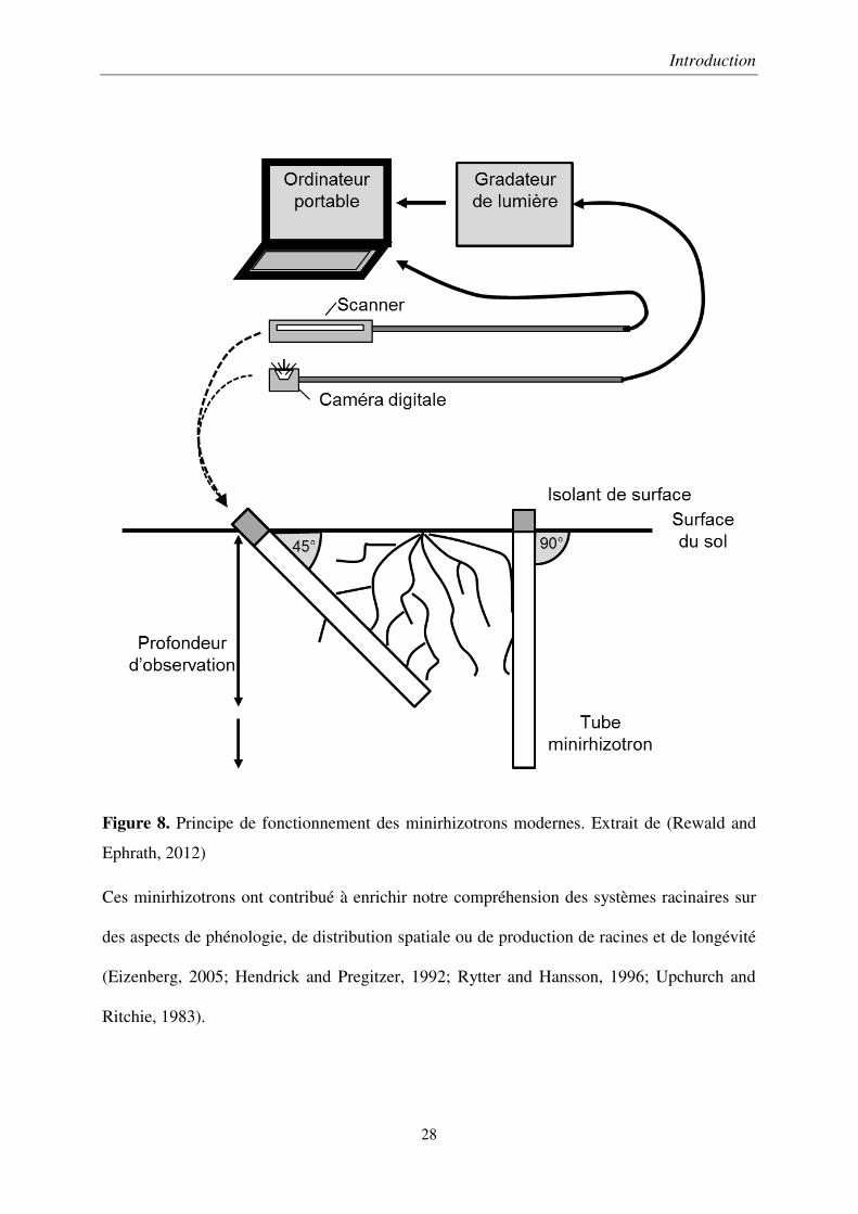
Figure 8. Principe de fonctionnement des minirhizotrons modernes. Extrait de (Rewald and

Ephrath, 2012)

Ces minirhizotrons ont contribué à enrichir notre compréhension des systèmes racinaires sur

des aspects de phénologie, de distribution spatiale ou de production de racines et de longévité

(Eizenberg, 2005; Hendrick and Pregitzer, 1992; Rytter and Hansson, 1996; Upchurch and

Ritchie, 1983).

Introduction

29

Une alternative possible, plus simple d’installation, est l’emploi de minirhizotrons. Ces outils

consistent en des tubes transparents installés dans le sol, dans lesquels on insère des caméras

pour capturer des images des racines en sous-sol, et ainsi suivre leur croissance. Différents

appareillages de capture d’images ont été mis au point (Rewald and Ephrath, 2012) et, de nos

jours, les deux systèmes les plus répandus sont basés sur des caméras vidéo (Withington et al.,

2003) ou des scanners (Liao et al., 2015; Munoz-Romero et al., 2010) (Figure 8). Bien qu’ils

permettent de quantifier les systèmes racinaires, les minirhizotrons sont encore peu utilisés

pour étudier l’enracinement des grandes cultures. Ce faible usage provient de la difficulté à

une installation convenable. En effet, un mauvais contact entre la paroi des tubes et le sol

induit un biais qui se manifeste par une prolifération des racines autour du tube. La fiabilité

des minirhizotrons dans un cadre de grandes cultures est donc encore peu documentée (Liao

et al., 2015). Ainsi, leur fiabilité et leur pertinence dans le cadre d’étude de phénotypage, par

exemple pour quantifier la réaction des systèmes racinaires de plants de blé soumis à un

déficit en intrants, sont explorées, sous forme d’article, dans le 2ème chapitre de cette thèse.

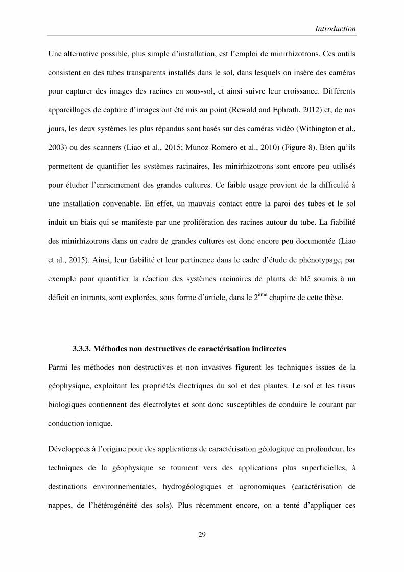
3.3.3. Méthodes non destructives de caractérisation indirectes

Parmi les méthodes non destructives et non invasives figurent les techniques issues de la

géophysique, exploitant les propriétés électriques du sol et des plantes. Le sol et les tissus

biologiques contiennent des électrolytes et sont donc susceptibles de conduire le courant par

conduction ionique.

Développées à l’origine pour des applications de caractérisation géologique en profondeur, les

techniques de la géophysique se tournent vers des applications plus superficielles, à

destinations environnementales, hydrogéologiques et agronomiques (caractérisation de

nappes, de l’hétérogénéité des sols). Plus récemment encore, on a tenté d’appliquer ces

Introduction

30

techniques au fonctionnement des plantes. Par exemple, la polarisation spontanée — la

différence naturelle de potentiel électrique entre une plante et le sol, — mesurée sur des arbres

(Quercus cerris) a été montrée corrélée aux variations de flux de sèves (aux flux

d’électrolytes) dûes à la transpiration et à la pression générée par les racines (Koppan et al.,

2002). Ces techniques ont également été appliquées à l’estimation et à la quantification des

racines dans le sol.

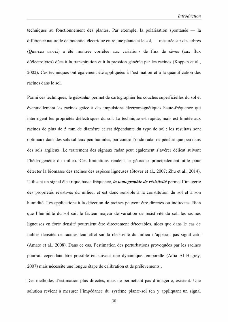
Parmi ces techniques, le géoradar permet de cartographier les couches superficielles du sol et

éventuellement les racines grâce à des impulsions électromagnétiques haute-fréquence qui

interrogent les propriétés diélectriques du sol. La technique est rapide, mais est limitée aux

racines de plus de 5 mm de diamètre et est dépendante du type de sol : les résultats sont

optimaux dans des sols sableux peu humides, par contre l’onde radar ne pénètre que peu dans

des sols argileux. Le traitement des signaux radar peut également s’avérer délicat suivant

l’hétérogénéité du milieu. Ces limitations rendent le géoradar principalement utile pour

détecter la biomasse des racines des espèces ligneuses (Stover et al., 2007; Zhu et al., 2014).

Utilisant un signal électrique basse fréquence, la tomographie de résistivité permet l’imagerie

des propriétés résistives du milieu, et est donc sensible à la constitution du sol et à son

humidité. Les applications à la détection de racines peuvent être directes ou indirectes. Bien

que l’humidité du sol soit le facteur majeur de variation de résistivité du sol, les racines

ligneuses en forte densité pourraient être directement détectables, alors que dans le cas de

faibles densités de racines leur effet sur la résistivité du milieu n’apparait pas significatif

(Amato et al., 2008). Dans ce cas, l’estimation des perturbations provoquées par les racines

pourrait cependant être possible en suivant une dynamique temporelle (Attia Al Hagrey,

2007) mais nécessite une longue étape de calibration et de prélèvements .

Des méthodes d’estimation plus directes, mais ne permettant pas d’imagerie, existent. Une

solution revient à mesurer l’impédance du système plante-sol (en y appliquant un signal

Introduction

31

électrique), reflétant les propriétés électrique du système, elles-mêmes potentiellement reliées

à la composition et la structure du sol et des tissus biologiques. De la même façon que la

maturation des fruits est quantifiable à travers l’impédance (Harker and Maindonald, 1994), il

serait possible d’analyser les propriétés électriques du système plante-sol pour en retrouver la

signature des racines. Généralement le sol et les tissus biologiques agissent comme des

résistances électriques (liées au flux d’électrolytes) ou comme des condensateurs (liées à

l’accumulation de charge à chaque interface).

4. Bases sur les techniques de mesures des racines

employées dans cette thèse

4.1. Les minirhizotrons

Les minirhizotrons ont été utilisés pour la mesure de traits architecturaux comme la

profondeur d’enracinement (Rasmussen et al., 2015), la distribution des racines, ces traits

entrant dans la résistance du blé à la sécheresse (Manschadi et al., 2006). La morphologie des

racines peut être aussi étudiée par minirhizotrons, tel le diamètre des racines (Withington et

al., 2003), un trait entrant en jeu dans l’efficacité de la capture de l’eau du sol. La production

de nouvelles racines et le renouvellement du système racinaire sont aussi observés avec cette

technique (Pilon et al., 2012), en particulier sur les dynamiques à court terme (Majdi et al.

2007). Les taux de mortalité observés au minirhizotron seraient comparables aux valeurs

issues d’autres techniques, notamment celles des méthodes isotopiques, lorsque le volume des

racines observées est considéré (Pritchard and Strand, 2008)— combinant ainsi longueurs et

diamètres observés. Les interactions avec la faune souterraine, le suivi de phénomènes de

parasitisme ont aussi fait l’objet d’étude par les minirhizotrons (Eizenberg, 2005).

Introduction

32

4.1.1. Tubes d'observation

4.1.1.1. Installation des tubes d'observation

Les minirhizotrons reposent sur l’installation de tubes transparents installés dans le sol. Le

type de sol et des facteurs spécifiques à l'espèce doivent être pris en compte lors de leur

installation. Pour éviter de perturber le sol et la végétation, il faut minimiser le piétinement

des zones étudiées. Ainsi, les minirhizotrons doivent être installés le plus tôt possible pour les

plantes annuelles (grandes cultures), de préférence à la levée.

Les sols caillouteux sont problématiques dans l’installation, à cause des complications de

forage qu’ils provoquent. Les trous d’insertion des minirhizotrons sont généralement obtenus

à l’aide de tarières (Munoz-Romero et al., 2010) ou de carottier (J. W. Hummel et al., 1989),

ou encore avec des dispositifs mécaniques de forage (Box et al., 1989; Kloeppel and Gower,

1995). Les tubes d’observations minirhizotrons sont généralement enfoncés jusqu’à 1 m de

profondeur. Afin de creuseur des trous rectilignes, un socle de support doit être positionné en

surface et peut occasionner des perturbations supplémentaires aux plantes en surface.

Afin d’éviter au mieux des artéfacts de la croissance racinaire, les tubes minirhizotrons

doivent idéalement être en contact parfait avec le sol. Toutefois, assurer un contact parfait tout

le long d’un tube est une opération difficile, et le diamètre du trou est un facteur déterminant

de l’installation. Ainsi, un forage au diamètre ajusté au diamètre du tube est la solution la plus

efficace, réduisant la chance de formation d’interstices entre le sol et la paroi du tube, et de

rotation des tubes lors de leur utilisation (Johnson et al., 2001). Bien qu’il facilite l'installation

des tubes minirhizotrons, un trou surdimensionné induit un écart entre la paroi du tube et le

sol, qui, même de taille réduite, constitue une zone de croissance préférentielle offrant peu de

résistance mécanique, ce qui peut augmenter artificiellement la colonisation par les racines

Introduction

33

(Volkmar, 1993). Un forage trop large peut nuire à la qualité des images obtenues du fait de la

condensation d’eau autour du tube ou de l’augmentation des risques d’effondrement des

parois du trou, provoquant une réorganisation du sol autour des tubes.

Hormis l’éventuelle compaction du sol provoquée par un trou trop ajusté (McMichael et al.,

1991) le phénomène de condensation autour du tube est réduit, facilitant l’observation des

racines. Le remblayage des trous surdimensionnés est généralement exclu, à cause de l‘effet

sur les traits racinaires observés de la densité et de la structure non-naturelle du sol (Kloeppel

and Gower, 1995).

4.1.1.2. Angle d'installation

Actuellement, les tubes minirhizotrons sont classiquement installés à un angle de 30° ou 45°,

bien que certaines études utilisent des tubes verticaux (90°) ou horizontaux (0°) (Johnson et

al., 2001). Les tubes posés avec un angle sont présentés comme permettant de mieux estimer

la distribution racinaire des grandes cultures que les tubes verticaux en réduisant l’effet de

croissance préférentielle le long du tube (Pagès and Bengough, 1997). Cet effet préférentiel

accru sur les tubes verticaux est probablement lié à l’infiltration de l’eau le long du tube et du

gravitropisme des racines, augmentant ainsi la tendance des racines à suivre le tube. Même si

aucune croissance préférentielle des racines de blé en fonction de l'angle d'insertion en sol

limono-sableux n’a été mise en évidence (Ephrath et al., 1999), les tubes en biais peuvent

intercepter en profondeur des plantes éloignées du lieu d’insertion du tube en surface,

permettant l’observation de racines provenant de plusieurs plantes comme celles d’un rang

dans une culture.

L’installation de tubes dans des milieux moins naturels, comme les lysimètres ou les

phytotrons semble être moins problématique. Ceux-ci permettent une pose plus aisée de tubes

Introduction

34

horizontaux pour maximiser la surface d’observation par profondeur de sol, bien qu’il semble

qu’il y ait une grande variation entre la surface supérieure des tubes et la surface inférieure

(Dubach and Russelle, 1995).

4.1.1.3. Protection du tube de la lumière et du climat

Il est nécessaire de fermer les deux extrémités du tube, avec un bouchon en pvc en partie

inférieure et un capuchon sur la partie émergente, pour éviter la présence d’eau à l’intérieur

du tube, que ce soit dû à la pluie ou aux remontées capillaires. Toutefois, l’eau peut aussi

s’accumuler par condensation, et ainsi il est important d’isoler la partie émergée des tubes de

la lumière et des fluctuations thermiques. Il est conseillé d’appliquer sur la surface des tubes

émergés un matériau isolant réfléchissant. De plus, cette isolation permet d’éviter

l’illumination de l’intérieur des tubes ainsi que les fluctuation thermiques qui peuvent affecter

la croissance racinaire (Levan et al., 1987).

4.1.1.4. Matériel et types de tubes d'observation minirhizotron

Différent matériaux ont été utilisés pour les tubes d’observation, et il apparait que les tubes

plastiques (Munoz-Romero et al., 2010) (en polyméthacrylate de méthyle [PMMA] ou en

polycarbonate) sont plus résistants que les tubes en verre (Kloeppel and Gower, 1995), face

aux phénomènes de gonflement et rétractation ou face au gel, tout en étant l’option la plus

économe. Bien que le verre et le plastique n’aient pas les mêmes propriétés optiques

(notamment dans la transmission), aucune différence significative sur les profils racinaires

obtenus avec les minirhizotrons n’a été constatée (Withington et al., 2003). Néanmoins, il

semble que la dynamique de production et de mortalité des racines soit possiblement impactée

par les différents matériaux constituant les tubes (Withington et al., 2003), les matériaux

plastiques pouvant conduire à une sous-estimation de la production de racines.

Introduction

35

4.1.2. Systèmes de capture d'images des racines

Dans la décennie écoulée, la technologie dédiée à l’acquisition d’images pour les

minirhizotrons a progressé en augmentant la vitesse d’acquisition et permettant la prise

d’images de plus grand format. Les systèmes d’acquisition utilisés de nos jours se divisent en

deux catégories : les caméras vidéo numériques et les scanners. Ces deux systèmes

d’acquisition sont instrumentés à l’aide d’ordinateurs portables équipés de logiciels dédiés,

gérant l’acquisition et l’étiquetage des images. Ils sont aussi équipés d’un système de guidage

qui permet à l'utilisateur de prendre des photos répétées au même endroit du sol.

4.1.2.1. Caméra vidéo numérique

Différentes tailles d'appareils existent, et le diamètre des tubes minirhizotrons doit être choisi

en fonction du diamètre du boîtier de la caméra. Dans les systèmes commerciaux, le système

le plus répandu est produit par Bartz (Carpinteria, CA, États-Unis). Les différentes

générations de caméra offrent différents niveaux de qualité d’images, certaines caméras

proposent un zoom optique 100×, permettant d’étudier en détails les racines (Eizenberg,

2005). Cependant la caméra ne couvre qu’une zone étroite du tube (<2 cm de large),

l’utilisation de caméra à plus large champ étant impossible en raison des déformations

optiques. Ainsi, des rotations de la caméra sont nécessaires pour obtenir tout le profil de sol et

de racines à une profondeur donnée. La plupart des systèmes basés sur des caméras vidéo

permettent un réglage manuel de la mise au point et de l’exposition et permettent l’adaptation

à des sources lumineuses avec un spectre lumineux spécifique, telles les sources infrarouges.

Introduction

36

4.1.2.2. Scanner rotatif

L’unique système basé sur un scanner rotatif existant est produit par CID Inc. (Camas, WA,

Etats-Unis). Un capteur CCD de scanner de bureau classique est monté sur un moteur rotatif

et permet de prendre des images sur 345° sur une profondeur de champ de l’ordre de 5mm.

Les images acquises sont décimétriques (20cm de large sur 22cm de haut), réduisant

drastiquement la quantité de prises de vues nécessaire pour la capture de l’intégralité de la

surface d’un tube. Avant chaque utilisation, le niveau de blanc du scanner doit être calibré.

Bien que la résolution maximale soit de 1200 ppp, la résolution de routine est typiquement de

300 ou 600 ppp afin de réduire le temps d’acquisition. La technologie CCD a pour

caractéristique intrinsèque une exposition homogène et une mise au point automatique,

facilitant l’usage. L’unique diamètre des scanners en vente implique l’utilisation de tubes de

70 mm de diamètre.

4.1.3. Données issues des minirhizotrons

Les minirhizotrons rendent possible l’analyse de nombreux traits des systèmes racinaires,

jusqu’à lors difficilement accessibles in situ en particulier la dynamique temporelle.

Néanmoins, l’interprétation de leurs données doit tenir compte des biais possibles associés à

la technique. Par exemple, les minirhizotrons pourraient sous-échantillonner le nombre de

classes de diamètres par rapport à un classement fait à partir de prélèvements destructifs

(Taylor et al., 2013). Une estimation fiable des diamètres des racines est importante car la

description de la dynamique racinaire est souvent basée sur des distributions de diamètres, qui

peuvent montrer un éventail de réponses aux traitements appliqués (Tingey et al., 1997;

Wilcox et al., 2004). Cependant, ce biais est surtout lié aux espèces présentant une grande

variabilité de diamètres, du fait que la quantité de racines de fort diamètre soit généralement

très sous-estimée. C’est le cas de la biomasse racinaire des arbres et arbustes qui n’est pas

Introduction

37

quantifiable globalement de façon fiable avec les minirhizotrons. Ces derniers sont plus

adaptés aux cultures annuelles, telles les céréales, dont les systèmes racinaires sont composés

essentiellement de racines aux diamètres inférieurs à 2 mm.

4.1.3.1. Données exploitables à partir des images

La mesure la plus simple est la présence (ou l’absence) de racines sur les images acquises, ce

qui permet de décrire la profondeur du sol exploré par le système racinaire sur le pourtour du

tube. Evidemment, aucune information n’est fournie sur les racines en dehors de la zone

d’échantillonnage.

La longueur de racines, communément mesurée sur les images de minirhizotrons, est souvent

divisée par la surface totale des tubes. On exprime alors la longueur de racines par unité de

surface (cm de racine par cm2 de surface de tube). La surface des racines elles-mêmes, par

l’estimation de leur diamètre, peut être observée et rapportée à la surface totale des tubes

(Johnson et al., 2001).

Certaines études utilisent le nombre de racines pour estimer la dynamique de croissance

(Fitter et al., 1998; Rytter and Rytter, 1998). Bien que le nombre de racines soit moins

sensible à la fréquence d'échantillonnage, il ne peut pas prendre en compte l’accroissement de

la longueur lié aux racines déjà présentes. Ainsi mesurer la longueur des racines semble une

meilleure option pour quantifier les dynamiques d’accroissement des systèmes racinaires, en

considérant l’orientation des racines afin de privilégier les racines impactant par dessus les

tubes minirhizotrons.

Introduction

38

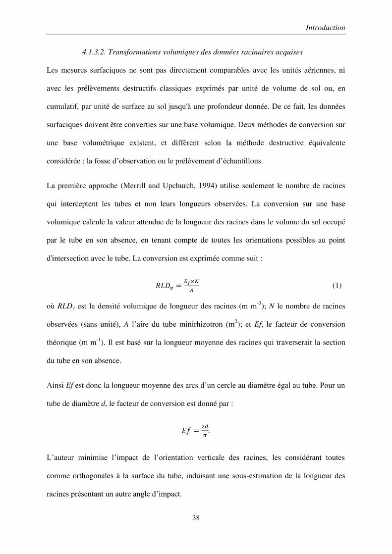
4.1.3.2. Transformations volumiques des données racinaires acquises

Les mesures surfaciques ne sont pas directement comparables avec les unités aériennes, ni

avec les prélèvements destructifs classiques exprimés par unité de volume de sol ou, en

cumulatif, par unité de surface au sol jusqu'à une profondeur donnée. De ce fait, les données

surfaciques doivent être converties sur une base volumique. Deux méthodes de conversion sur

une base volumétrique existent, et diffèrent selon la méthode destructive équivalente

considérée : la fosse d’observation ou le prélèvement d’échantillons.

La première approche (Merrill and Upchurch, 1994) utilise seulement le nombre de racines

qui interceptent les tubes et non leurs longueurs observées. La conversion sur une base

volumique calcule la valeur attendue de la longueur des racines dans le volume du sol occupé

par le tube en son absence, en tenant compte de toutes les orientations possibles au point

d'intersection avec le tube. La conversion est exprimée comme suit :

𝑅𝐿𝐷𝑣 =𝐸𝑓×𝑁

𝐴 (1)

où RLDv est la densité volumique de longueur des racines (m m-3); N le nombre de racines

observées (sans unité), A l’aire du tube minirhizotron (m2); et Ef, le facteur de conversion

théorique (m m-1). Il est basé sur la longueur moyenne des racines qui traverserait la section

du tube en son absence.

Ainsi Ef est donc la longueur moyenne des arcs d’un cercle au diamètre égal au tube. Pour un

tube de diamètre d, le facteur de conversion est donné par :

𝐸𝑓 =2𝑑

𝜋.

L’auteur minimise l’impact de l’orientation verticale des racines, les considérant toutes

comme orthogonales à la surface du tube, induisant une sous-estimation de la longueur des

racines présentant un autre angle d’impact.

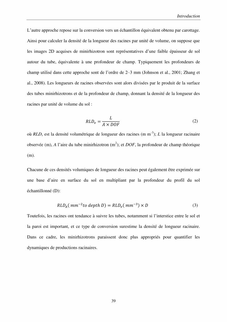
Introduction

39

L’autre approche repose sur la conversion vers un échantillon équivalent obtenu par carottage.

Ainsi pour calculer la densité de la longueur des racines par unité de volume, on suppose que

les images 2D acquises de minirhizotron sont représentatives d’une faible épaisseur de sol

autour du tube, équivalente à une profondeur de champ. Typiquement les profondeurs de

champ utilisé dans cette approche sont de l’ordre de 2–3 mm (Johnson et al., 2001; Zhang et

al., 2008). Les longueurs de racines observées sont alors divisées par le produit de la surface

des tubes minirhizotrons et de la profondeur de champ, donnant la densité de la longueur des

racines par unité de volume du sol :

𝑅𝐿𝐷𝑣 =𝐿

𝐴 × 𝐷𝑂𝐹 (2)

où RLDv est la densité volumétrique de longueur des racines (m m-3); L la longueur racinaire

observée (m), A l’aire du tube minirhizotron (m2); et DOF, la profondeur de champ théorique

(m).

Chacune de ces densités volumiques de longueur des racines peut également être exprimée sur

une base d’aire en surface du sol en multipliant par la profondeur du profil du sol

échantillonné (D):

𝑅𝐿𝐷𝐴( 𝑚𝑚−2𝑡𝑜 𝑑𝑒𝑝𝑡ℎ 𝐷) = 𝑅𝐿𝐷𝑣( 𝑚𝑚−3) × 𝐷 (3)

Toutefois, les racines ont tendance à suivre les tubes, notamment si l’interstice entre le sol et

la paroi est important, et ce type de conversion surestime la densité de longueur racinaire.

Dans ce cadre, les minirhizotrons paraissent donc plus appropriés pour quantifier les

dynamiques de productions racinaires.

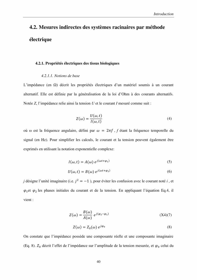
Introduction

40

4.2. Mesures indirectes des systèmes racinaires par méthode

électrique

4.2.1. Propriétés électriques des tissus biologiques

4.2.1.1. Notions de base

L’impédance (en Ω) décrit les propriétés électriques d’un matériel soumis à un courant

alternatif. Elle est définie par la généralisation de la loi d’Ohm à des courants alternatifs.

Notée Z, l’impédance relie ainsi la tension U et le courant I mesuré comme suit :

𝑍(𝜔) =𝑈(𝜔, 𝑡)

𝐼(𝜔, 𝑡) (4)

où ω est la fréquence angulaire, défini par 𝜔 = 2𝜋𝑓 , f étant la fréquence temporelle du

signal (en Hz). Pour simplifier les calculs, le courant et la tension peuvent également être

exprimés en utilisant la notation exponentielle complexe:

𝐼(𝜔, 𝑡) = 𝐴(𝜔) 𝑒𝑗(𝜔𝑡+𝜑1) (5)

𝑈(𝜔, 𝑡) = 𝐵(𝜔) 𝑒𝑗(𝜔𝑡+𝜑2) (6)

j désigne l’unité imaginaire (i.e. 𝑗2 = −1 ), pour éviter les confusion avec le courant noté i , et

𝜑1et 𝜑2 les phases initiales du courant et de la tension. En appliquant l’équation Eq.4, il

vient :

𝑍(𝜔) =𝐵(𝜔)𝐴(𝜔)

𝑒𝑗(𝜑2−𝜑1) (X4)(7)

𝑍(𝜔) = 𝑍0(𝜔) 𝑒𝑗𝜑0 (8)

On constate que l’impédance possède une composante réelle et une composante imaginaire

(Eq. 8). 𝑍0 décrit l’effet de l’impédance sur l’amplitude de la tension mesurée, et 𝜑0 celui du

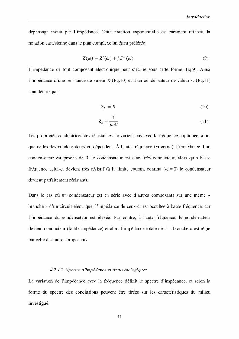
Introduction

41

déphasage induit par l’impédance. Cette notation exponentielle est rarement utilisée, la

notation cartésienne dans le plan complexe lui étant préférée :

𝑍(𝜔) = 𝑍′(𝜔) + 𝑗 𝑍′′(𝜔) (9)

L’impédance de tout composant électronique peut s’écrire sous cette forme (Eq.9). Ainsi

l’impédance d’une résistance de valeur R (Eq.10) et d’un condensateur de valeur C (Eq.11)

sont décrits par :

𝑍𝑅 = 𝑅 (10)

𝑍𝑐 =1

𝑗𝜔𝐶 (11)

Les propriétés conductrices des résistances ne varient pas avec la fréquence appliquée, alors

que celles des condensateurs en dépendent. À haute fréquence (ω grand), l‘impédance d’un

condensateur est proche de 0, le condensateur est alors très conducteur, alors qu’à basse

fréquence celui-ci devient très résistif (à la limite courant continu (ω = 0) le condensateur

devient parfaitement résistant).

Dans le cas où un condensateur est en série avec d’autres composants sur une même «

branche » d’un circuit électrique, l’impédance de ceux-ci est occultée à basse fréquence, car

l’impédance du condensateur est élevée. Par contre, à haute fréquence, le condensateur

devient conducteur (faible impédance) et alors l’impédance totale de la « branche » est régie

par celle des autre composants.

4.2.1.2. Spectre d’impédance et tissus biologiques

La variation de l’impédance avec la fréquence définit le spectre d’impédance, et selon la

forme du spectre des conclusions peuvent être tirées sur les caractéristiques du milieu

investigué.

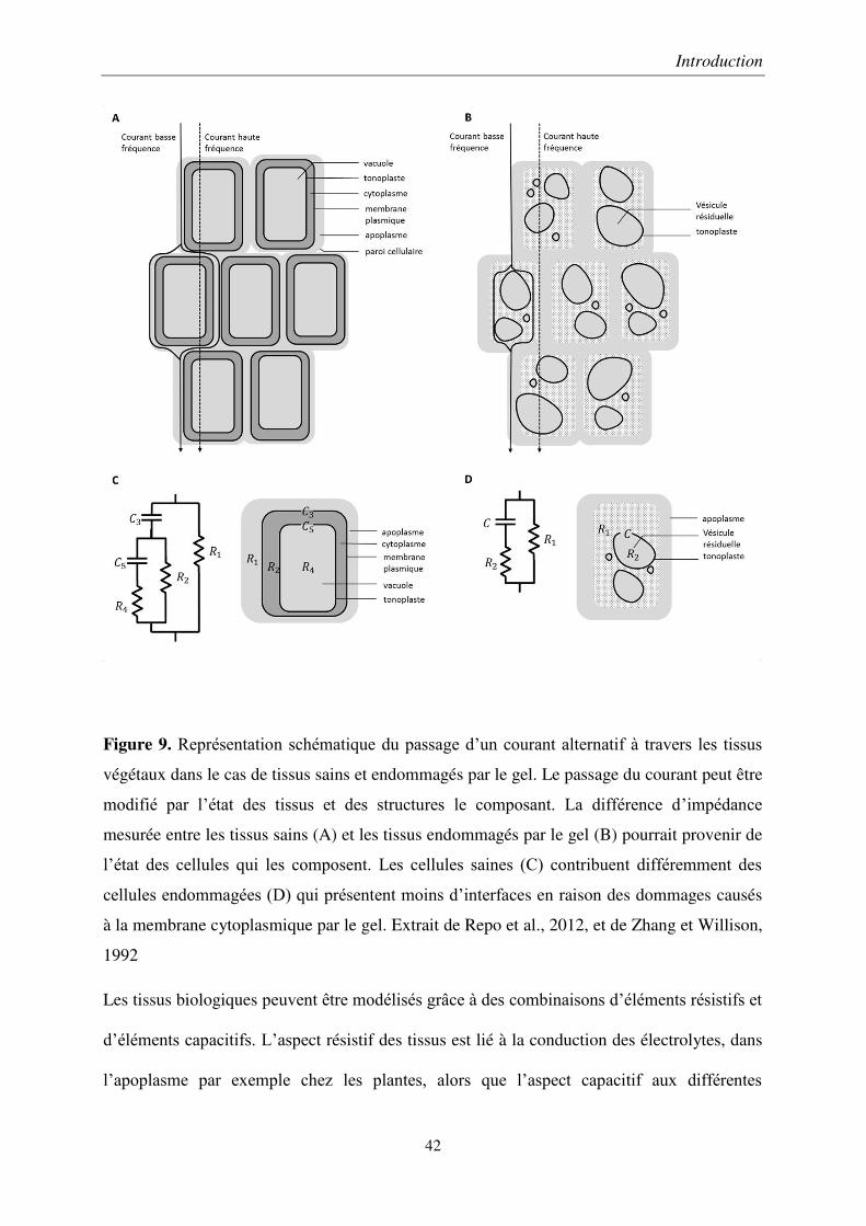
Introduction

42

Figure 9. Représentation schématique du passage d’un courant alternatif à travers les tissus

végétaux dans le cas de tissus sains et endommagés par le gel. Le passage du courant peut être

modifié par l’état des tissus et des structures le composant. La différence d’impédance

mesurée entre les tissus sains (A) et les tissus endommagés par le gel (B) pourrait provenir de

l’état des cellules qui les composent. Les cellules saines (C) contribuent différemment des

cellules endommagées (D) qui présentent moins d’interfaces en raison des dommages causés

à la membrane cytoplasmique par le gel. Extrait de Repo et al., 2012, et de Zhang et Willison,

1992

Les tissus biologiques peuvent être modélisés grâce à des combinaisons d’éléments résistifs et

d’éléments capacitifs. L’aspect résistif des tissus est lié à la conduction des électrolytes, dans

l’apoplasme par exemple chez les plantes, alors que l’aspect capacitif aux différentes

Introduction

43

fréquences décrit les phénomènes d’accumulation d’électrolytes aux interfaces, par exemple

au niveau des membranes plasmiques. Il est possible de modéliser chaque interface par un

condensateur et chaque milieu conducteur par une résistance, la mise en série d’un

condensateur avec un autre élément correspondant au passage d’une interface (membrane).

Une des conséquences de la caractéristique alternative du champ électrique appliqué est que le

passage du courant peut interroger différents compartiments formant le tissu végétal suivant la

fréquence (Figure 9-A et C). En raison de leur bicouche lipidique, les membranes cellulaires

ne peuvent pas être traversées par un courant alternatif basse fréquence, agissant ainsi comme

des condensateurs. Dans cette situation, le courant circule dans l'espace apoplastique et

l'impédance totale mesurée est alors principalement liée à la résistance de ce continuum. À

mesure que la fréquence augmente, les membranes cellulaires deviennent conductrices, et à

des fréquences suffisamment élevées (> 100 kHz), l'impédance totale est composée d'une

combinaison parallèle des résistances intracellulaire (symplastique) et extracellulaire

(apoplastique).

Ainsi Zhang and Willison (1992) ont modélisé l’effet d’une congélation/décongélation sur des

plants de carottes, par deux circuits différents. Le premier modèle décrivant des cellules

végétales intactes contient deux interfaces (Figure 9 C) — la membrane plasmique et le

tonoplaste — , alors que le second modèle décrit une cellule dont la membrane plasmique a

explosée et ne possède donc plus qu’une seule interface (Figure 9 D)

On peut aussi modéliser ce phénomène de dispersion à travers les variations de la permittivité

du milieu. Cela revient à décrire l’effet des tissus biologiques lorsqu’ils sont utilisés comme

isolants, comme dans un condensateur. Puisque la permittivité est une grandeur intensive (qui

ne dépend pas de la taille du système), son utilisation en modélisation permet de considérer

Introduction

44

simplement des circuits distribués — caractérisés par un circuit élémentaire répété selon la

taille du système. Ainsi, la permittivité est décrite par un nombre complexe :

𝜀 = 𝜀′ − 𝑗𝜀′′ = 𝜀′ − 𝑗𝜎𝜔

(12)

où ε’ et ε’’ sont des parties réelles et imaginaires de la permittivité (F.m-1). D'une manière

générale, ε’ se rapporte à la fraction de l'énergie électrique qui est stockée dans les

condensateurs, et ε’’ à la fraction dissipée par conduction.

4.2.2. Application de la mesure de l’impédance aux systèmes racinaires

4.2.2.1. Rapide historique

L’exploration de l’utilisation de la mesure capacitive pour estimer la biomasse racinaire a

débuté avec Oldřich Chloupek au début des années 1970. Ainsi, il mis au point une première

expérience (Chloupek, 1972) dont le but était de quantifier des traits racinaires de plantes de

différentes espèces — maïs (Zea mays. L.), tournesols (Helianthus annuus L.), colza

(Brassica napus L.), avoine (Avena sativa. L.) et oignon (Allium cepa. L.) — toutes cultivées

dans des pots remplis avec des substrats sableux ou argileux, portés à leur humidité maximum

avant chaque mesure. L’auteur observa une relation linéaire entre la capacité électrique du

système et la masse racinaire du système. Le montage électrique consistait en 2 électrodes,

l’une placée sur la plante, et l’autre placée dans le substrat, les deux reliées à un appareil de

mesure de capacité.

Dans des expérimentations ultérieures (Chloupek, 1977), le même auteur confirme cette

relation empirique au laboratoire et en condition de plein champ sur ce panel d’espèces. De

fortes corrélations entre la masse racinaire et la capacité furent observées, que ce soit au

laboratoire sur des pommes de terre (Solanum tuberosum) ou au champ sur des tournesols

Introduction

45

(Helianthus annuus L.). L’auteur conclut que cet effet capacitif est lié à la polarisation des

cellules des tissus biologiques des racines (Schwan, 1959), et que le sol joue un rôle

négligeable à cause de sa grande conductivité.

Plus tard, d’autres expérimentations sur des plantes (Medicago sativa) en situation de culture

montrent que l’efficacité de la méthode capacitive diminue avec le développement des plantes

et n’est plus fiable lorsque les stades jeunes sont dépassés (Kendall et al., 1982).

À partir d’expérimentations en milieu contrôlé (hydroponie), et en se basant sur quelques

hypothèses concernant les dimensions caractéristiques des racines, Dalton (1995) formule la

contribution de chaque racine à la capacité électrique totale du système racinaire.

Néanmoins, l’application au champ semble pourtant poser des difficultés (Preston et al.,

2004), et il semble que les paramètres de la relation linéaire soient spécifiques aux espèces

(Aulen and Shipley, 2012). De même, les observations au champ indiquent que la méthode est

sensible à l’humidité du sol, cette dernière jouant un rôle prépondérant dans la variance

inexpliquée des relations. En étendant cette méthode de mesure sur une gamme de fréquences,

l’exploitation du spectre obtenu en modélisant des systèmes électriques équivalents a permis

d’isoler la réponse spécifique des racines (Ozier-Lafontaine and Bajazet, 2005), réduisant

ainsi pour partie l’impact du milieu de culture sur la variabilité des prédictions de biomasse

racinaire. Malgré cet effort d’amélioration de la prédiction de biomasse, les paramètres de la

relation linéaire entre biomasse et capacité électrique ne sont pas établis. Autrement dit, il

n’existe pas de formule donnant les valeurs des paramètres de cette relation linéaire en

fonction du système sol-plante mesuré, et il reste nécessaire d’effectuer des prélèvements

destructifs pour les déterminer.

Introduction

46

Dalton (1995) a introduit une représentation et une théorie expliquant l’influence de la

biomasse racinaire sur la transmission du courant plante-sol et son effet sur la capacité

mesurée. Longtemps admise, cette théorie a été remise en question récemment plus ou moins

profondément (Ellis et al., 2013 ; Dietrich et al., 2012). Dans ce dernier cas, ce n’est plus la

biomasse racinaire mais seulement la section des racines en contact avec le substrat de culture

qui influe sur la capacité mesurée. Ces différents modèles sont présentés ci-dessous.

4.2.2.2. Le modèle de Dalton

Dalton (1995) introduit une théorie sur la relation linéaire expérimentale masse racinaire -

capacité, en proposant un modèle électrique équivalent, à l’échelle d’une racine, pour une

section élémentaire. L’auteur décrit un élément de racine comme un condensateur cylindrique,

le conducteur interne étant la sève du xylème et le phloème — tissus du système vasculaire

des plantes — le conducteur externe étant l’interface sol-racine. Les tissus parenchymatiques

du cortex et de la stèle, entre le système vasculaire et l’épiderme, forment le matériel

diélectrique (Figure 10 A). En calculant la capacité d’un tel condensateur, dans le cas où le

rayon interne est petit devant l’épaisseur de diélectrique, et en ajoutant que la surface des

racines est corrélée à leur masse — impliquant que le diamètre et la densité de masse des

racines de plantes d’une même espèce soient peu variables, les variations de diamètres sont

plus faible qu’un ordre de grandeur — l’auteur dérive une relation linéaire entre masse

racinaire et capacité électrique.

Par ailleurs l’effet de position de l’électrode « plante » est évaluée et une longueur

élémentaire de tige est ainsi identifiée comme une série de circuit RC mis en série. Sans

donner de détails sur les hypothèses sous-jacentes à la conductivité des différentes structures

Introduction

47

racinaires (conductivité du xylème par rapport conductivité du sol), l’auteur met l’accent sur

l’importance d’avoir un sol humide, pour maximiser la surface d’interface sol-plante.

Une extension utilisant une analyse du spectre d’impédance (Ozier-Lafontaine and Bajazet,

2005) a été proposée pour isoler l’impédance du système racinaire de l’impédance du sol, afin

d’affiner la prédiction de masse racinaire.

4.2.2.3. Le modèle d’Ellis et al.

Dans le modèle de Dalton (1995), le diamètre des racines entre en jeu dans le modèle

électrique équivalent d’une racine, i.e. le condensateur cylindrique. Dans ses expériences,

Dalton ne mesure pas ce diamètre et ne peut donc pas évaluer l’impédance d’un segment de

racine, ni la permittivité des tissus qui le compose. Afin d’évaluer cette valeur de permittivité,

et d’évaluer la théorie de Dalton, Ellis propose d’évaluer les corrélations entre la capacité, la

longueur, la surface, et la masse chez le pois (Vicia Faba). Les auteurs introduisent un nouvel

estimateur de la masse de racine, basé sur une relation empirique liant la longueur, la capacité

et la masse volumique des racines (Figure 10 B). En appliquant le modèle des condensateurs

cylindriques et à l’aide de mesures de diamètres, les auteurs parviennent à déterminer une

valeur de permittivité des tissues racinaires satisfaisante (εr = 68) au regard des permittivités

de la cellulose (εr = 7,6) et de l’eau (εr = 80). Les auteurs concluent que la capacité électrique

est un estimateur de la longueur racinaire, en précisant que la quasi-intégralité du système

racinaire forme un système électrique interconnecté — appuyant ainsi l’importance d’avoir un

sol humide.

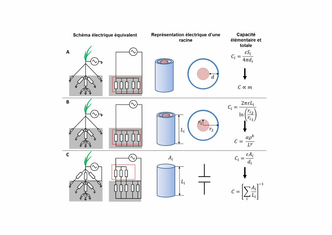
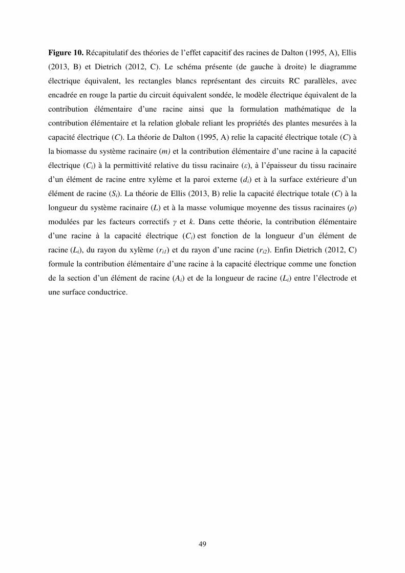
49

Figure 10. Récapitulatif des théories de l’effet capacitif des racines de Dalton (1995, A), Ellis

(2013, B) et Dietrich (2012, C). Le schéma présente (de gauche à droite) le diagramme

électrique équivalent, les rectangles blancs représentant des circuits RC parallèles, avec

encadrée en rouge la partie du circuit équivalent sondée, le modèle électrique équivalent de la

contribution élémentaire d’une racine ainsi que la formulation mathématique de la

contribution élémentaire et la relation globale reliant les propriétés des plantes mesurées à la

capacité électrique (C). La théorie de Dalton (1995, A) relie la capacité électrique totale (C) à

la biomasse du système racinaire (m) et la contribution élémentaire d’une racine à la capacité

électrique (Ci) à la permittivité relative du tissu racinaire (ε), à l’épaisseur du tissu racinaire

d’un élément de racine entre xylème et la paroi externe (di) et à la surface extérieure d’un

élément de racine (Si). La théorie de Ellis (2013, B) relie la capacité électrique totale (C) à la

longueur du système racinaire (L) et à la masse volumique moyenne des tissus racinaires (ρ)

modulées par les facteurs correctifs γ et k. Dans cette théorie, la contribution élémentaire

d’une racine à la capacité électrique (Ci) est fonction de la longueur d’un élément de

racine (Li), du rayon du xylème (ri1) et du rayon d’une racine (ri2). Enfin Dietrich (2012, C)

formule la contribution élémentaire d’une racine à la capacité électrique comme une fonction

de la section d’un élément de racine (Ai) et de la longueur de racine (Li) entre l’électrode et

une surface conductrice.

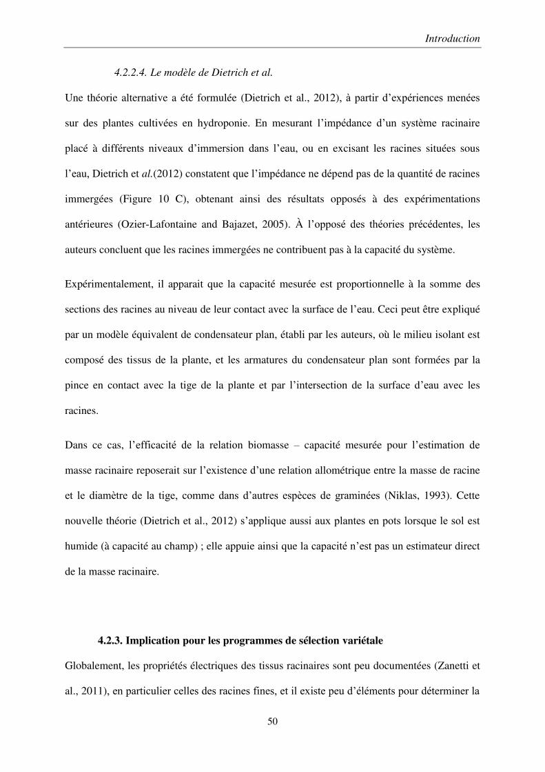
Introduction

50

4.2.2.4. Le modèle de Dietrich et al.

Une théorie alternative a été formulée (Dietrich et al., 2012), à partir d’expériences menées

sur des plantes cultivées en hydroponie. En mesurant l’impédance d’un système racinaire

placé à différents niveaux d’immersion dans l’eau, ou en excisant les racines situées sous

l’eau, Dietrich et al.(2012) constatent que l’impédance ne dépend pas de la quantité de racines

immergées (Figure 10 C), obtenant ainsi des résultats opposés à des expérimentations

antérieures (Ozier-Lafontaine and Bajazet, 2005). À l’opposé des théories précédentes, les

auteurs concluent que les racines immergées ne contribuent pas à la capacité du système.

Expérimentalement, il apparait que la capacité mesurée est proportionnelle à la somme des

sections des racines au niveau de leur contact avec la surface de l’eau. Ceci peut être expliqué

par un modèle équivalent de condensateur plan, établi par les auteurs, où le milieu isolant est

composé des tissus de la plante, et les armatures du condensateur plan sont formées par la

pince en contact avec la tige de la plante et par l’intersection de la surface d’eau avec les

racines.

Dans ce cas, l’efficacité de la relation biomasse – capacité mesurée pour l’estimation de

masse racinaire reposerait sur l’existence d’une relation allométrique entre la masse de racine

et le diamètre de la tige, comme dans d’autres espèces de graminées (Niklas, 1993). Cette

nouvelle théorie (Dietrich et al., 2012) s’applique aussi aux plantes en pots lorsque le sol est

humide (à capacité au champ) ; elle appuie ainsi que la capacité n’est pas un estimateur direct

de la masse racinaire.

4.2.3. Implication pour les programmes de sélection variétale

Globalement, les propriétés électriques des tissus racinaires sont peu documentées (Zanetti et

al., 2011), en particulier celles des racines fines, et il existe peu d’éléments pour déterminer la

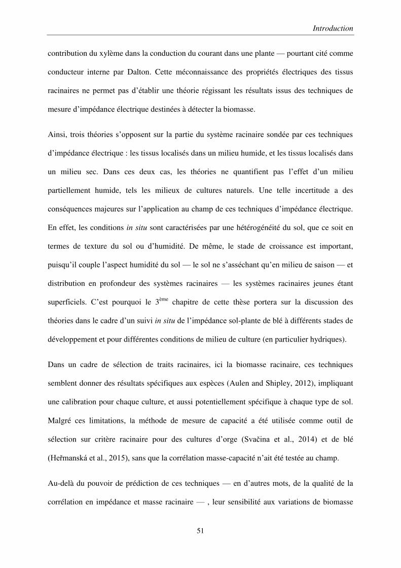
Introduction

51

contribution du xylème dans la conduction du courant dans une plante — pourtant cité comme

conducteur interne par Dalton. Cette méconnaissance des propriétés électriques des tissus

racinaires ne permet pas d’établir une théorie régissant les résultats issus des techniques de

mesure d’impédance électrique destinées à détecter la biomasse.

Ainsi, trois théories s’opposent sur la partie du système racinaire sondée par ces techniques

d’impédance électrique : les tissus localisés dans un milieu humide, et les tissus localisés dans

un milieu sec. Dans ces deux cas, les théories ne quantifient pas l’effet d’un milieu

partiellement humide, tels les milieux de cultures naturels. Une telle incertitude a des

conséquences majeures sur l’application au champ de ces techniques d’impédance électrique.

En effet, les conditions in situ sont caractérisées par une hétérogénéité du sol, que ce soit en

termes de texture du sol ou d’humidité. De même, le stade de croissance est important,

puisqu’il couple l’aspect humidité du sol — le sol ne s’asséchant qu’en milieu de saison — et

distribution en profondeur des systèmes racinaires — les systèmes racinaires jeunes étant

superficiels. C’est pourquoi le 3ème chapitre de cette thèse portera sur la discussion des

théories dans le cadre d’un suivi in situ de l’impédance sol-plante de blé à différents stades de

développement et pour différentes conditions de milieu de culture (en particulier hydriques).

Dans un cadre de sélection de traits racinaires, ici la biomasse racinaire, ces techniques

semblent donner des résultats spécifiques aux espèces (Aulen and Shipley, 2012), impliquant

une calibration pour chaque culture, et aussi potentiellement spécifique à chaque type de sol.

Malgré ces limitations, la méthode de mesure de capacité a été utilisée comme outil de

sélection sur critère racinaire pour des cultures d’orge (Svačina et al., 2014) et de blé

(Heřmanská et al., 2015), sans que la corrélation masse-capacité n’ait été testée au champ.

Au-delà du pouvoir de prédiction de ces techniques — en d’autres mots, de la qualité de la

corrélation en impédance et masse racinaire — , leur sensibilité aux variations de biomasse

Introduction

52

racinaire est rarement discutée, bien qu’il s’agisse d’un point crucial pour son utilisation en

tant que capteur. Ainsi, l’optimisation du dispositif de mesure est capitale, autant pour assurer

un outil fiable destiné à la sélection variétale que pour standardiser ces techniques

d’impédance électrique. C’est pourquoi l’objet du 1er chapitre du manuscrit sera de déterminer

un montage optimal de mesure de ces techniques d’impédance électrique appliquées aux

plantes.

53

Objectifs et résultats

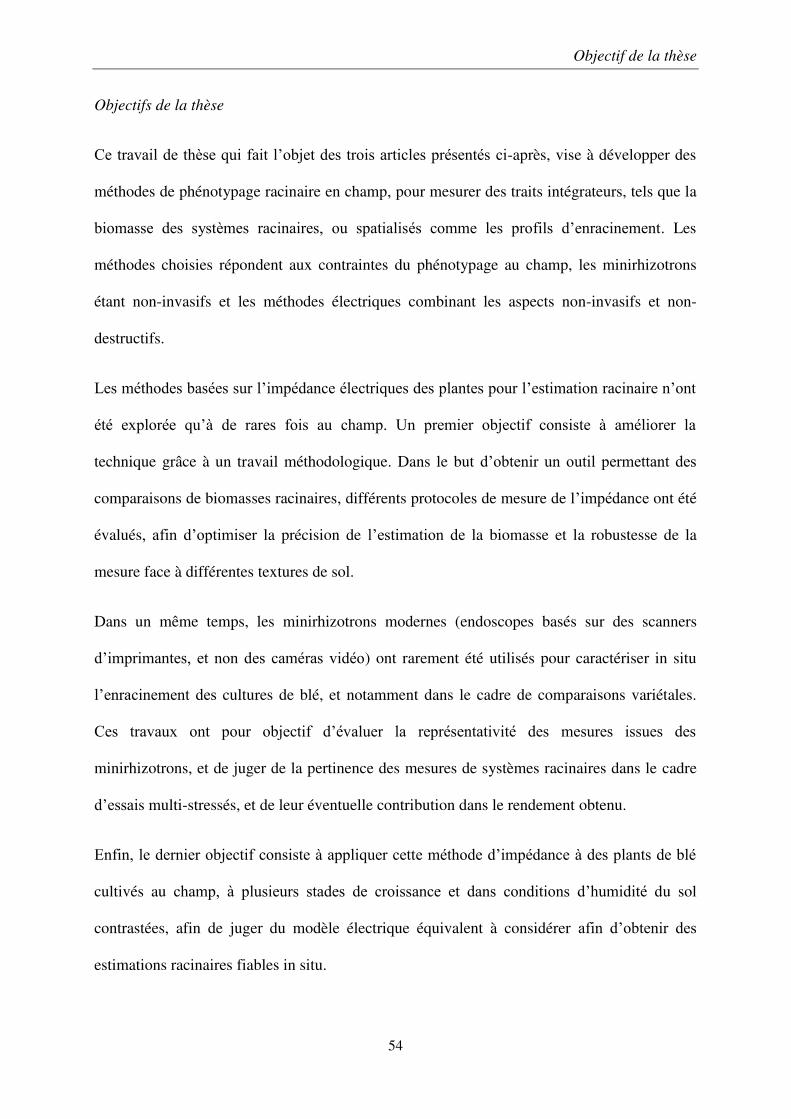
Objectif de la thèse

54

Objectifs de la thèse

Ce travail de thèse qui fait l’objet des trois articles présentés ci-après, vise à développer des

méthodes de phénotypage racinaire en champ, pour mesurer des traits intégrateurs, tels que la

biomasse des systèmes racinaires, ou spatialisés comme les profils d’enracinement. Les

méthodes choisies répondent aux contraintes du phénotypage au champ, les minirhizotrons

étant non-invasifs et les méthodes électriques combinant les aspects non-invasifs et non-

destructifs.

Les méthodes basées sur l’impédance électriques des plantes pour l’estimation racinaire n’ont

été explorée qu’à de rares fois au champ. Un premier objectif consiste à améliorer la

technique grâce à un travail méthodologique. Dans le but d’obtenir un outil permettant des

comparaisons de biomasses racinaires, différents protocoles de mesure de l’impédance ont été

évalués, afin d’optimiser la précision de l’estimation de la biomasse et la robustesse de la

mesure face à différentes textures de sol.

Dans un même temps, les minirhizotrons modernes (endoscopes basés sur des scanners

d’imprimantes, et non des caméras vidéo) ont rarement été utilisés pour caractériser in situ

l’enracinement des cultures de blé, et notamment dans le cadre de comparaisons variétales.

Ces travaux ont pour objectif d’évaluer la représentativité des mesures issues des

minirhizotrons, et de juger de la pertinence des mesures de systèmes racinaires dans le cadre

d’essais multi-stressés, et de leur éventuelle contribution dans le rendement obtenu.

Enfin, le dernier objectif consiste à appliquer cette méthode d’impédance à des plants de blé

cultivés au champ, à plusieurs stades de croissance et dans conditions d’humidité du sol

contrastées, afin de juger du modèle électrique équivalent à considérer afin d’obtenir des

estimations racinaires fiables in situ.

55

Chapitre 1 : Analyse comparative des

méthodes électriques pour l'estimation rapide

de la biomasse racinaire

François Postic Claude Doussan 

  

Plant Methods, 2016   

     

Chapitre 1

56

Ce premier chapitre, présenté sous forme d’ article, vise à mettre au point le dispositif idéal de

mesure électrique pour la détection de racines. Nos mesures ont été effectuées en suivant les

recommandations de Dalton (1995), c’est-à-dire de porter les substrats à capacité au champ.

Ces expérimentations en pots de faibles volume nous ont permis de déterminer quelle

configuration de mesure — en termes de nombre de terminaux, électrode de contact à la

plante, fréquence du signal, variable électrique — choisir pour obtenir le meilleur estimateur

de masse racinaire que ce soit en terme de prédiction, ou de sensibilité. Sur les différents sols

de culture, il apparait que la capacité électrique en parallèle est le meilleur estimateur de

masse racinaire. Cet article a été publié dans Plant Methods.

Postic and Doussan Plant Methods (2016) 12:33 DOI 10.1186/s13007-016-0133-7

METHODOLOGY

Benchmarking electrical methods for rapid estimation of root biomassFrançois Postic1,2 and Claude Doussan2*

Abstract

Background: To face climate change and subsequent rainfall instabilities, crop breeding strategies now include root traits phenotyping. Rapid estimation of root traits in controlled conditions can be achieved by using parallel electrical capacitance and its linear correlation with root dry mass. The aim of the present study was to improve robustness and efficiency of methods based on capacitance and other electrical variables, such as serial/parallel resistance, conduct-ance, impedance or reactance. Using different electrode configurations and stem contact electrodes, we have meas-ured the electrical impedance spectra of wheat plants grown in pots filled with three types of soil.

Results: For each configuration, parallel capacitance and other linearly independent electrical variables were com-puted and their quality as root dry mass estimator was evaluated by a ‘sensitivity score’ that we derived from Pear-son’s correlation coefficient r and linear regression parameters. The highest sensitivity score was obtained by parallel capacitance at an alternating current frequency of 116 Hz in three-terminal configuration. Using a clamp, instead of a needle, as a stem electrode did not significantly affect the capacitance measurements. Finally, in handheld LCR meter equivalent conditions, capacitance had the highest sensitivity score and determination coefficient (r2 = 0.52) at 10 kHz frequency.

Conclusion: Our benchmarking of linear correlations between different electrical variables and root dry mass ena-bles to determine more coherent practices for ensuring a sensitive and robust root dry mass estimation, including in handheld LCR meter conditions. This would enhance the value of electrical capacitance as a tool for screening crops in relation with root systems in breeding programs.

Keywords: Wheat, Triticum durum, Root mass, Electrical impedance spectrometry, Capacitance, Terminal configuration, Contact electrode

© 2016 The Author(s). This article is distributed under the terms of the Creative Commons Attribution 4.0 International License (http://creativecommons.org/licenses/by/4.0/), which permits unrestricted use, distribution, and reproduction in any medium, provided you give appropriate credit to the original author(s) and the source, provide a link to the Creative Commons license, and indicate if changes were made. The Creative Commons Public Domain Dedication waiver (http://creativecommons.org/publicdomain/zero/1.0/) applies to the data made available in this article, unless otherwise stated.

BackgroundHigher cereal yield are needed to feed a growing popu-lation in the near future [1]. However, partly as a con-sequence of climate change, yield of cereals tends to level off in different parts of the world as crops are fac-ing more often sub-optimal conditions (water, nutrients, temperature) for growth [2]. The root system is a central actor in alleviating stress when inputs are suboptimal or limiting [3] and, in such conditions, water/nutrient cap-ture is directly linked to root distribution and activity in soil in relation with the temporal pattern of resource

availability. For example, depending on rainfall pattern, root proliferation in shallow soil layer may exhaust soil water too quickly before anthesis, detrimentally to yield, while deep rooting would be advantageous in capturing deep stored water at post-anthesis, and beneficial to yield [4–7]. Both modelling and field experiments showed that such a deep rooting could indeed increase or maintain grain yield for rainfed wheat [8, 9]. Nevertheless, regard-less of the root distribution pattern, increase/decrease in root density and biomass would be a factor influenc-ing yield, depending on the environmental conditions [6, 7]. Besides, the early vigour and growth of root systems also plays a major role in drought tolerance, as shown for barley [10]. Whereas high-throughput phenotyping is developing extensively [11, 12], especially on aerial parts,

Open Access

Plant Methods

*Correspondence: claude.doussan@paca.inra.fr 2 UMR EMMAH, INRA, UAPV, Domaine Saint-Paul, Site Agroparc, 84914 Avignon, FranceFull list of author information is available at the end of the article

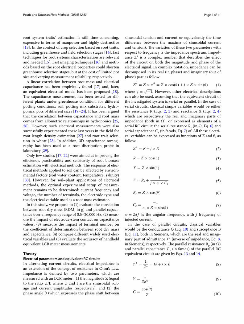
Page 2 of 11Postic and Doussan Plant Methods (2016) 12:33

root system traits’ estimation is still time-consuming, expensive in terms of manpower and highly destructive [13]. In the context of crop selection based on root traits, including greenhouse and field selection stages [14], fast techniques for root systems characterization are relevant and needed [15]. Fast imaging techniques [16] and meth-ods based on the root electrical properties could shorten greenhouse selection stages, but at the cost of limited pot size and varying measurement reliability, respectively.

A linear correlation between root mass and electrical capacitance has been empirically found [17] and, later, an equivalent electrical model has been proposed [18]. The capacitance measurement has been tested for dif-ferent plants under greenhouse condition, for different potting conditions: soil, potting mix substrates, hydro-ponics, pots of different sizes [19–24]. It has been argued that the correlation between capacitance and root mass comes from allometric relationships in hydroponics [25, 26]. However, such electrical measurements were also successfully experimented these last years in the field for root length density estimation [27] and root trait selec-tion in wheat [28]. In addition, 3D capacitance tomog-raphy has been used as a root distribution probe in laboratory [29].

Only few studies [17, 22] were aimed at improving the efficiency, practicability and sensitivity of root biomass estimation with electrical methods. The response of elec-trical methods applied to soil can be affected by environ-mental factors (soil water content, temperature, salinity) [30]. However, for soil–plant applications of electrical methods, the optimal experimental setup of measure-ment remains to be determined: current frequency and voltage, the number of terminals, the electrode type and the electrical variable used as a root mass estimator.

In this study, we propose to (1) evaluate the correlation between root dry mass (RDM, in g) and parallel capaci-tance over a frequency range of 0.5–20,000 Hz, (2) meas-ure the impact of electrode-stem contact on capacitance values, (3) measure the impact of terminal number on the coefficient of determination between root dry mass and capacitance, (4) compare different widely used elec-trical variables and (5) evaluate the accuracy of handheld equivalent LCR meter measurements.

TheoryElectrical parameters and equivalent RC circuitsIn alternating current circuits, electrical impedance is an extension of the concept of resistance in Ohm’s Law. Impedance is defined by two parameters, which are measured with an LCR meter: (1) the magnitude Z (equal to the ratio U/I, where U and I are the sinusoidal volt-age and current amplitudes respectively), and (2) the phase angle θ (which expresses the phase shift between

sinusoidal tension and current or equivalently the time difference between the maxima of sinusoidal current and tension). The variation of these two parameters with respect to frequency is the impedance spectrum. Imped-ance Z∗ is a complex number that describes the effect of the circuit on both the magnitude and phase of the electrical signal. In complex notation, impedance can be decomposed in its real (in phase) and imaginary (out of phase) part as follow:

where j =√

−1. However, other electrical descriptions can also be used, assuming that the equivalent circuit of the investigated system is serial or parallel. In the case of serial circuits, classical simple variables would be either the resistance R (Eqs.  2, 3) and reactance X (Eqs.  2, 4) which are respectively the real and imaginary parts of impedance (both in Ω), or expressed as elements of a serial RC circuit: the serial resistance Rs (in Ω, Eq. 6) and serial capacitance Cs (in farads, Eq. 7) of. All these electri-cal variables can be expressed as functions of Z and θ, as follow:

ω = 2π f is the angular frequency, with f frequency of injected current.

In the case of parallel circuits, classical variables would be the conductance G (Eq. 10) and susceptance B (Eq. 11), both in Siemens, which are the real and imagi-nary part of admittance Y∗ (inverse of impedance, Eq. 8, in Siemens), respectively. The parallel resistance Rp (in Ω) and parallel capacitance Cp (in farads) of the parallel RC equivalent circuit are given by Eqs. 13 and 14.

(1)Z∗ = Z × ejθ = Z × cos(θ) + j × Z × sin(θ)

(2)Z∗ = R + j × X

(3)R = Z × cos(θ)

(4)X = Z × sin(θ)

(5)Z = Rs +1

j × ω × Cs

(6)Rs = Z × cos(θ)

(7)Cs =−1

ω × Z × sin(θ)

(8)Y ∗ =1

Z∗ = G + j × B

(9)Y =1

Zejθ

(10)G =cos(θ)

Z

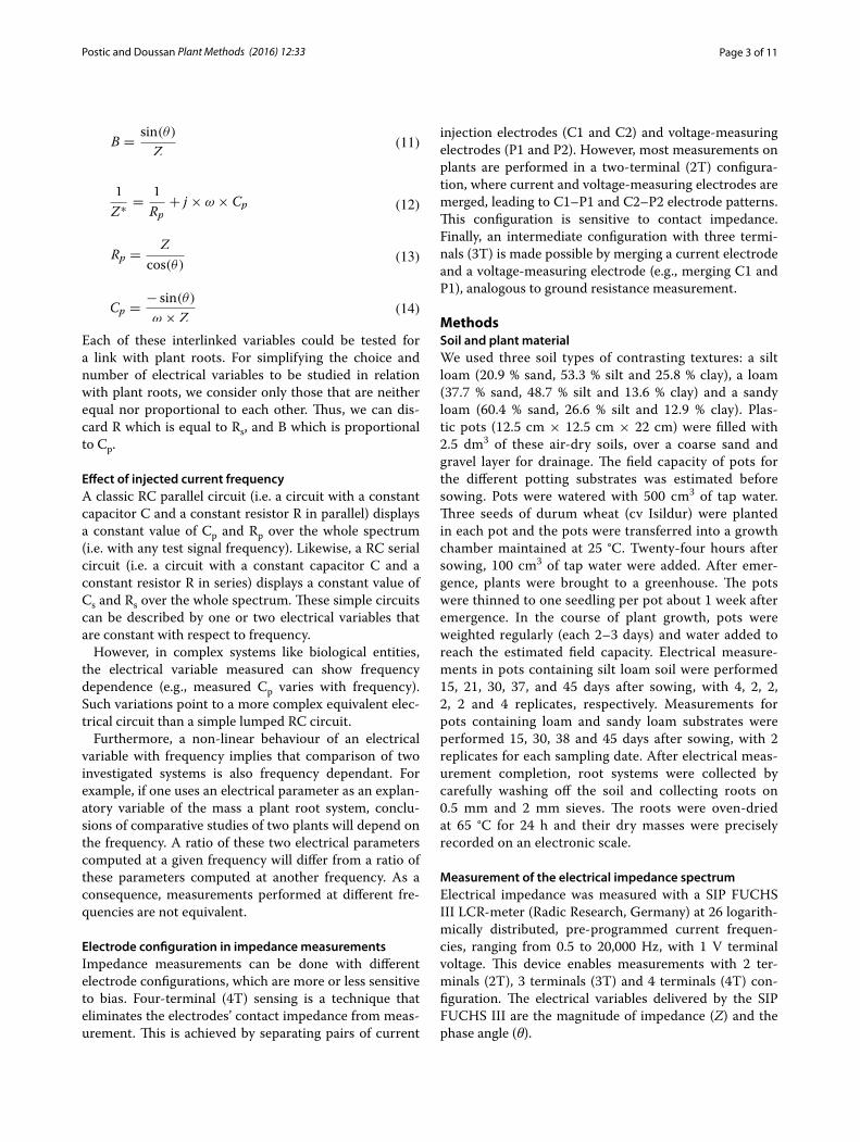
Page 3 of 11Postic and Doussan Plant Methods (2016) 12:33

Each of these interlinked variables could be tested for a link with plant roots. For simplifying the choice and number of electrical variables to be studied in relation with plant roots, we consider only those that are neither equal nor proportional to each other. Thus, we can dis-card R which is equal to Rs, and B which is proportional to Cp.

Effect of injected current frequencyA classic RC parallel circuit (i.e. a circuit with a constant capacitor C and a constant resistor R in parallel) displays a constant value of Cp and Rp over the whole spectrum (i.e. with any test signal frequency). Likewise, a RC serial circuit (i.e. a circuit with a constant capacitor C and a constant resistor R in series) displays a constant value of Cs and Rs over the whole spectrum. These simple circuits can be described by one or two electrical variables that are constant with respect to frequency.

However, in complex systems like biological entities, the electrical variable measured can show frequency dependence (e.g., measured Cp varies with frequency). Such variations point to a more complex equivalent elec-trical circuit than a simple lumped RC circuit.

Furthermore, a non-linear behaviour of an electrical variable with frequency implies that comparison of two investigated systems is also frequency dependant. For example, if one uses an electrical parameter as an explan-atory variable of the mass a plant root system, conclu-sions of comparative studies of two plants will depend on the frequency. A ratio of these two electrical parameters computed at a given frequency will differ from a ratio of these parameters computed at another frequency. As a consequence, measurements performed at different fre-quencies are not equivalent.

Electrode configuration in impedance measurementsImpedance measurements can be done with different electrode configurations, which are more or less sensitive to bias. Four-terminal (4T) sensing is a technique that eliminates the electrodes’ contact impedance from meas-urement. This is achieved by separating pairs of current

(11)B =sin(θ)

Z

(12)1

Z∗ =1

Rp+ j × ω × Cp

(13)Rp =Z

cos(θ)

(14)Cp =− sin(θ)

ω × Z

injection electrodes (C1 and C2) and voltage-measuring electrodes (P1 and P2). However, most measurements on plants are performed in a two-terminal (2T) configura-tion, where current and voltage-measuring electrodes are merged, leading to C1–P1 and C2–P2 electrode patterns. This configuration is sensitive to contact impedance. Finally, an intermediate configuration with three termi-nals (3T) is made possible by merging a current electrode and a voltage-measuring electrode (e.g., merging C1 and P1), analogous to ground resistance measurement.

MethodsSoil and plant materialWe used three soil types of contrasting textures: a silt loam (20.9 % sand, 53.3 % silt and 25.8 % clay), a loam (37.7 % sand, 48.7 % silt and 13.6 % clay) and a sandy loam (60.4 % sand, 26.6 % silt and 12.9 % clay). Plas-tic pots (12.5 cm × 12.5 cm × 22 cm) were filled with 2.5  dm3 of these air-dry soils, over a coarse sand and gravel layer for drainage. The field capacity of pots for the different potting substrates was estimated before sowing. Pots were watered with 500  cm3 of tap water. Three seeds of durum wheat (cv Isildur) were planted in each pot and the pots were transferred into a growth chamber maintained at 25  °C. Twenty-four hours after sowing, 100 cm3 of tap water were added. After emer-gence, plants were brought to a greenhouse. The pots were thinned to one seedling per pot about 1 week after emergence. In the course of plant growth, pots were weighted regularly (each 2–3 days) and water added to reach the estimated field capacity. Electrical measure-ments in pots containing silt loam soil were performed 15, 21, 30, 37, and 45  days after sowing, with 4, 2, 2, 2, 2 and 4 replicates, respectively. Measurements for pots containing loam and sandy loam substrates were performed 15, 30, 38 and 45 days after sowing, with 2 replicates for each sampling date. After electrical meas-urement completion, root systems were collected by carefully washing off the soil and collecting roots on 0.5  mm and 2  mm sieves. The roots were oven-dried at 65  °C for 24 h and their dry masses were precisely recorded on an electronic scale.

Measurement of the electrical impedance spectrumElectrical impedance was measured with a SIP FUCHS III LCR-meter (Radic Research, Germany) at 26 logarith-mically distributed, pre-programmed current frequen-cies, ranging from 0.5 to 20,000 Hz, with 1 V terminal voltage. This device enables measurements with 2 ter-minals (2T), 3 terminals (3T) and 4 terminals (4T) con-figuration. The electrical variables delivered by the SIP FUCHS III are the magnitude of impedance (Z) and the phase angle (θ).

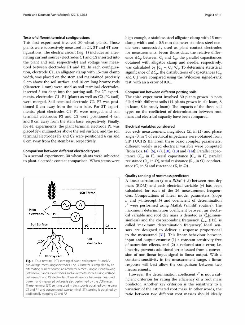
Page 4 of 11Postic and Doussan Plant Methods (2016) 12:33

Tests of different terminal configurationsThis first experiment involved 30 wheat plants. Those plants were successively measured in 2T, 3T and 4T con-figurations. The electric circuit (Fig. 1) includes an alter-nating current source (electrodes C1 and C2 inserted into the plant and soil, respectively) and voltage was meas-ured between electrodes P1 and P2. In each configura-tion, electrode C1, an alligator clamp with 15-mm clamp width, was placed on the stem and maintained precisely 5 cm above the soil surface, and 10 cm long bronze rods (diameter 1 mm) were used as soil terminal electrodes, inserted 3 cm deep into the potting soil. For 2T experi-ments, electrodes C1–P1 (plant) as well as C2–P2 (soil) were merged. Soil terminal electrode C2–P2 was posi-tioned 8  cm away from the stem base. For 3T experi-ments, plant electrodes C1–P1 were merged, and soil terminal electrodes P2 and C2 were positioned 4  cm and 8 cm away from the stem base, respectively. Finally, for 4T experiments, the plant terminal electrode P1 was placed few millimetres above the soil surface, and the soil terminal electrodes P2 and C2 were positioned 4 cm and 8 cm away from the stem base, respectively.

Comparison between different electrode typesIn a second experiment, 30 wheat plants were subjected to plant-electrode contact comparison. When stems were

high enough, a stainless steel alligator clamp with 15 mm clamp width and a 0.5 mm diameter stainless steel nee-dle were successively used as plant contact electrodes for measurements. From those data, the relative differ-ence ΔCp between Cc and Cn, the parallel capacitances obtained with alligator clamp and needle, respectively, was calculated by |Cc − Cn|/Cc. To determine statistical significance of ΔCp, the distributions of capacitances (Cn and Cc) were compared using the Wilcoxon signed-rank test, with an α error of 0.01.

Comparison between different potting soilsThe third experiment involved 30 plants grown in pots filled with different soils (14 plants grown in silt loam, 8 in loam, 8 in sandy loam). The impacts of the three soil types on the coefficient of determination between root mass and electrical capacity have been compared.

Electrical variables consideredFor each measurement, magnitude (Z, in Ω) and phase angle (θ, in °) of electrical impedance were obtained from SIP FUCHS III. From these basic complex parameters, different widely used electrical variable were computed [from Eqs. (4), (6), (7), (10), (13) and (14)]: Parallel capac-itance (Cp, in F), serial capacitance (Cs, in F), parallel resistance (Rp, in Ω), serial resistance (Rs, in Ω), conduct-ance (G, in S) and reactance (X, in Ω).

Quality ranking of root mass predictorsA linear correlation (y = a RDM + b) between root dry mass (RDM) and each electrical variable (y) has been calculated for each of the 26 measurement frequen-cies. Computations of linear model parameters (slope a and y-intercept b) and coefficient of determination r2 were performed using Matlab (‘nlinfit’ routine). The maximum determination coefficient between an electri-cal variable and root dry mass is denoted as rmax

2 (dimen-sionless) and the corresponding frequency, fmax (Hz), is called ‘maximum determination frequency’. Ideal sen-sors are designed to deliver a response proportional to the measurand [31]. This linear behaviour between input and output ensures: (1) a constant sensitivity free of saturation effects, and (2) a reduced static error, i.e. linearity prevents additional error issued from a conver-sion of non-linear input signal to linear output. With a constant sensitivity in the measurement range, a linear response will best allow the comparison between two measurements.

However, the determination coefficient r2 is not a suf-ficient criterion for rating the efficiency of a root mass predictor. Another key criterion is the sensitivity to a variation of the estimated root mass. In other words, the ratio between two different root masses should ideally

Fig. 1 Four-terminal (4T) sensing of plant–soil system. P1 and P2 are voltage-measuring electrodes. The LCR meter is simplified by an alternating current source, an ammeter A measuring current flowing between C1 and C2 electrodes and a voltmeter V measuring voltage between P1 and P2 electrodes. Phase difference between measured current and measured voltage is also performed by the LCR meter. Three-terminal (3T) sensing used in this study is obtained by merging C1 and P1, and conventional two-terminal (2T) sensing is obtained by additionally merging C2 and P2

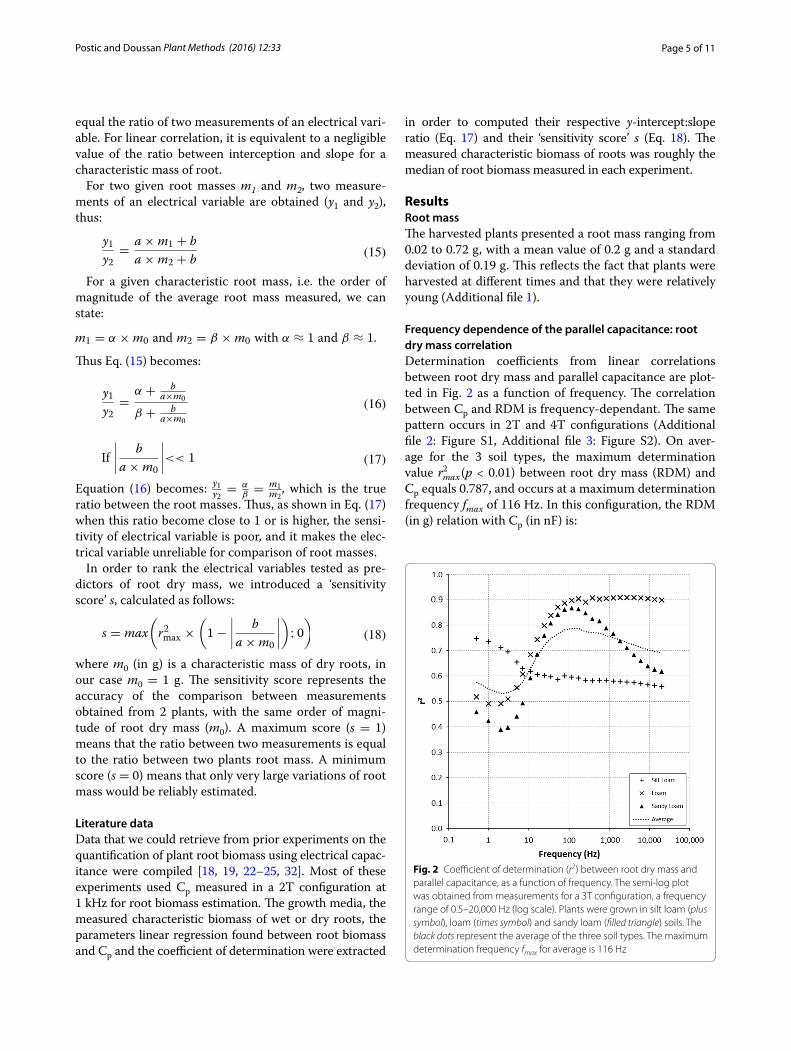
Page 5 of 11Postic and Doussan Plant Methods (2016) 12:33

equal the ratio of two measurements of an electrical vari-able. For linear correlation, it is equivalent to a negligible value of the ratio between interception and slope for a characteristic mass of root.

For two given root masses m1 and m2, two measure-ments of an electrical variable are obtained (y1 and y2), thus:

For a given characteristic root mass, i.e. the order of magnitude of the average root mass measured, we can state:

Thus Eq. (15) becomes:

Equation  (16) becomes: y1y2 = αβ

= m1

m2, which is the true

ratio between the root masses. Thus, as shown in Eq. (17) when this ratio become close to 1 or is higher, the sensi-tivity of electrical variable is poor, and it makes the elec-trical variable unreliable for comparison of root masses.

In order to rank the electrical variables tested as pre-dictors of root dry mass, we introduced a ‘sensitivity score’ s, calculated as follows:

where m0 (in g) is a characteristic mass of dry roots, in our case m0 = 1  g. The sensitivity score represents the accuracy of the comparison between measurements obtained from 2 plants, with the same order of magni-tude of root dry mass (m0). A maximum score (s =  1) means that the ratio between two measurements is equal to the ratio between two plants root mass. A minimum score (s = 0) means that only very large variations of root mass would be reliably estimated.

Literature dataData that we could retrieve from prior experiments on the quantification of plant root biomass using electrical capac-itance were compiled [18, 19, 22–25, 32]. Most of these experiments used Cp measured in a 2T configuration at 1 kHz for root biomass estimation. The growth media, the measured characteristic biomass of wet or dry roots, the parameters linear regression found between root biomass and Cp and the coefficient of determination were extracted

(15)y1

y2=

a × m1 + b

a × m2 + b

m1 = α × m0 and m2 = β × m0 with α ≈ 1 and β ≈ 1.

(16)y1

y2=

α + ba×m0

β + ba×m0

(17)If

�

�

�

�

b

a × m0

�

�

�

�

<< 1

(18)s = max

�

r2max �

1 −�

�

�

�

b

a × m0

�

�

�

�

�

; 0�

in order to computed their respective y-intercept:slope ratio (Eq.  17) and their ‘sensitivity score’ s (Eq.  18). The measured characteristic biomass of roots was roughly the median of root biomass measured in each experiment.

ResultsRoot massThe harvested plants presented a root mass ranging from 0.02 to 0.72 g, with a mean value of 0.2 g and a standard deviation of 0.19 g. This reflects the fact that plants were harvested at different times and that they were relatively young (Additional file 1).

Frequency dependence of the parallel capacitance: root dry mass correlationDetermination coefficients from linear correlations between root dry mass and parallel capacitance are plot-ted in Fig. 2 as a function of frequency. The correlation between Cp and RDM is frequency-dependant. The same pattern occurs in 2T and 4T configurations (Additional file  2: Figure S1, Additional file  3: Figure S2). On aver-age for the 3 soil types, the maximum determination value rmax

2 (p < 0.01) between root dry mass (RDM) and Cp equals 0.787, and occurs at a maximum determination frequency fmax of 116 Hz. In this configuration, the RDM (in g) relation with Cp (in nF) is:

Fig. 2 Coefficient of determination (r2) between root dry mass and parallel capacitance, as a function of frequency. The semi-log plot was obtained from measurements for a 3T configuration, a frequency range of 0.5–20,000 Hz (log scale). Plants were grown in silt loam (plus symbol), loam (times symbol) and sandy loam (filled triangle) soils. The black dots represent the average of the three soil types. The maximum determination frequency fmax for average is 116 Hz

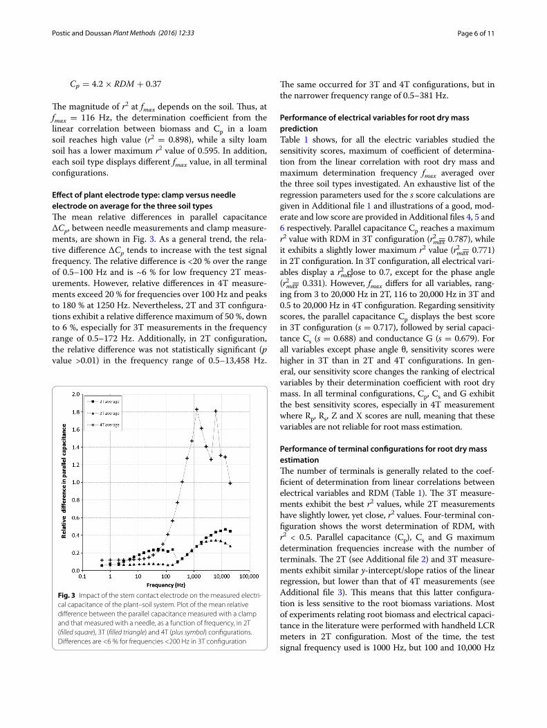
Page 6 of 11Postic and Doussan Plant Methods (2016) 12:33

The magnitude of r2 at fmax depends on the soil. Thus, at fmax =  116  Hz, the determination coefficient from the linear correlation between biomass and Cp in a loam soil reaches high value (r2 =  0.898), while a silty loam soil has a lower maximum r2 value of 0.595. In addition, each soil type displays different fmax value, in all terminal configurations.

Effect of plant electrode type: clamp versus needle electrode on average for the three soil typesThe mean relative differences in parallel capacitance ΔCp, between needle measurements and clamp measure-ments, are shown in Fig. 3. As a general trend, the rela-tive difference ΔCp tends to increase with the test signal frequency. The relative difference is <20 % over the range of 0.5–100 Hz and is ~6 % for low frequency 2T meas-urements. However, relative differences in 4T measure-ments exceed 20 % for frequencies over 100 Hz and peaks to 180 % at 1250 Hz. Nevertheless, 2T and 3T configura-tions exhibit a relative difference maximum of 50 %, down to 6 %, especially for 3T measurements in the frequency range of 0.5–172 Hz. Additionally, in 2T configuration, the relative difference was not statistically significant (p value >0.01) in the frequency range of 0.5–13,458  Hz.

Cp = 4.2 × RDM + 0.37 The same occurred for 3T and 4T configurations, but in the narrower frequency range of 0.5–381 Hz.

Performance of electrical variables for root dry mass predictionTable  1 shows, for all the electric variables studied the sensitivity scores, maximum of coefficient of determina-tion from the linear correlation with root dry mass and maximum determination frequency fmax averaged over the three soil types investigated. An exhaustive list of the regression parameters used for the s score calculations are given in Additional file 1 and illustrations of a good, mod-erate and low score are provided in Additional files 4, 5 and 6 respectively. Parallel capacitance Cp reaches a maximum r2 value with RDM in 3T configuration (rmax

2 = 0.787), while it exhibits a slightly lower maximum r2 value (rmax

2 = 0.771) in 2T configuration. In 3T configuration, all electrical vari-ables display a rmax

2 close to 0.7, except for the phase angle (rmax

2 = 0.331). However, fmax differs for all variables, rang-ing from 3 to 20,000 Hz in 2T, 116 to 20,000 Hz in 3T and 0.5 to 20,000 Hz in 4T configuration. Regarding sensitivity scores, the parallel capacitance Cp displays the best score in 3T configuration (s = 0.717), followed by serial capaci-tance Cs (s = 0.688) and conductance G (s = 0.679). For all variables except phase angle θ, sensitivity scores were higher in 3T than in 2T and 4T configurations. In gen-eral, our sensitivity score changes the ranking of electrical variables by their determination coefficient with root dry mass. In all terminal configurations, Cp, Cs and G exhibit the best sensitivity scores, especially in 4T measurement where Rp, Rs, Z and X scores are null, meaning that these variables are not reliable for root mass estimation.

Performance of terminal configurations for root dry mass estimationThe number of terminals is generally related to the coef-ficient of determination from linear correlations between electrical variables and RDM (Table 1). The 3T measure-ments exhibit the best r2 values, while 2T measurements have slightly lower, yet close, r2 values. Four-terminal con-figuration shows the worst determination of RDM, with r2  <  0.5. Parallel capacitance (Cp), Cs and G maximum determination frequencies increase with the number of terminals. The 2T (see Additional file 2) and 3T measure-ments exhibit similar y-intercept/slope ratios of the linear regression, but lower than that of 4T measurements (see Additional file  3). This means that this latter configura-tion is less sensitive to the root biomass variations. Most of experiments relating root biomass and electrical capaci-tance in the literature were performed with handheld LCR meters in 2T configuration. Most of the time, the test signal frequency used is 1000 Hz, but 100 and 10,000 Hz

Fig. 3 Impact of the stem contact electrode on the measured electri-cal capacitance of the plant–soil system. Plot of the mean relative difference between the parallel capacitance measured with a clamp and that measured with a needle, as a function of frequency, in 2T (filled square), 3T (filled triangle) and 4T (plus symbol) configurations. Differences are <6 % for frequencies <200 Hz in 3T configuration

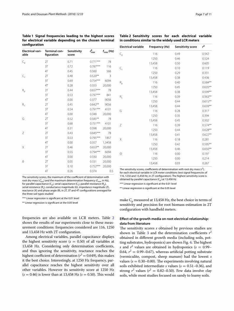
Page 7 of 11Postic and Doussan Plant Methods (2016) 12:33

frequencies are also available on LCR meters. Table  2 shows the results of our experiments close to these meas-urement conditions: frequencies considered are 116, 1250 and 13,458 Hz with 2T configuration.

Among electrical variables, parallel capacitance displays the highest sensitivity score (s =  0.50) of all variables at 13,458  Hz. Considering only determination coefficients, and thus ignoring the sensitivity, reactance reaches the highest coefficient of determination (r2 = 0.649), this makes it the best choice. Interestingly, at 1250 Hz frequency, par-allel capacitance reaches the highest sensitivity over all other variables. However its sensitivity score at 1250 Hz (s = 0.46) is lower than at 13,458 Hz (s = 0.50). This would

make Cp measured at 13,458 Hz, the best choice in terms of sensitivity and precision for root biomass estimation in 2T configuration with handheld meters.

Effect of the growth media on root electrical relationship: data from literatureThe sensitivity scores s obtained by previous studies are shown in Table  3 and the determination coefficients r2 obtained in different growth media (including soils, pot-ting substrates, hydroponics) are shown Fig. 4. The highest s and r2 values are obtained in hydroponics (s =  0.99–0.64, r2 = 0.99–0.67), whereas artificial potting substrate (vermiculite, compost, sheep manure) had the lowest s values (s = 0.30–0.00). The experiments involving natural soils exhibited intermediate s values (s = 0.51–0.36), and strong r2 values (r2 =  0.82–0.50). Few data involve clay soils, while most studies focused on sandy to loamy soils.

Table 1 Signal frequencies leading to  the highest scores for electrical variable depending on  the chosen terminal configuration

The sensitivity scores, the maximum of the coefficient of determination with root dry mass (rma x

2 ) and the maximum determination frequency (fmax, in Hz), for parallel capacitance (Cp), serial capacitance (Cs), parallel resistance (Rp), serial resistance (Rs), conductance magnitude (G), impedance magnitude (Z), reactance (X) and phase angle (θ), in 2T, 3T and 4T configurations averaged for the three soil types studied

*** Linear regression is significant at the 0.01 level

** Linear regression is significant at the 0.05 level

Electrical vari-able

Terminal con-figuration

Sensitivity score

rmax2 fmax (Hz)

Cp 2T 0.71 0.771*** 78

3T 0.72 0.787*** 116

4T 0.45 0.560 566

Cs 2T 0.48 0.520** 3

3T 0.69 0.754*** 6094

4T 0.28 0.353 20,000

Rp 2T 0.44 0.657*** 78

3T 0.53 0.797*** 841

4T 0.00 0.377 9056

Rs 2T 0.45 0.642** 9056

3T 0.54 0.791*** 4101

4T 0.00 0.348 20,000

G 2T 0.52 0.585** 78

3T 0.68 0.751*** 4101

4T 0.31 0.398 20,000

Z 2T 0.43 0.645*** 78

3T 0.53 0.795*** 1857

4T 0.00 0.357 1,3458

X 2T 0.46 0.653** 20,000

3T 0.55 0.794*** 6094

4T 0.00 0.330 20,000

θ 2T 0.05 0.331 20,000

3T 0.10 0.752*** 20,000

4T 0.26 0.374 0.5

Table 2 Sensitivity scores for  each electrical variable in conditions similar to the widely used LCR meters

The sensitivity scores, coefficients of determination with root dry mass (r2), for each electrical variable in LCR meter conditions (test signal frequencies of 116, 1250 and 13,458 Hz, in 2T configuration). The highest sensitivity score is obtained by parallel capacitance (Cp) at 13,458 Hz

*** Linear regression is significant at the 0.01 level

** Linear regression is significant at the 0.05 level

Electrical variable Frequency (Hz) Sensitivity score r2

Cp 116 0.49 0.542

1250 0.46 0.524

13,458 0.50 0.605

Cs 116 0.10 0.119

1250 0.29 0.331

13,458 0.38 0.436

Rp 116 0.40 0.584**

1250 0.45 0.635**

13,458 0.38 0.599**

Rs 116 0.39 0.563**

1250 0.44 0.615**

13,458 0.44 0.639**

G 116 0.28 0.317

1250 0.35 0.394

13,458 0.45 0.502

Z 116 0.39 0.574**

1250 0.44 0.628**

13,458 0.41 0.622**

X 116 0.18 0.281

1250 0.42 0.595**

13,458 0.46 0.650**

Θ 116 0.00 0.197

1250 0.00 0.214

13,458 0.03 0.267

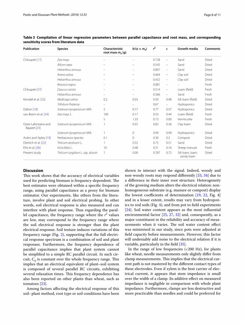
Page 8 of 11Postic and Doussan Plant Methods (2016) 12:33

DiscussionThis work shows that the accuracy of electrical variables used for predicting biomass is frequency-dependent. The best estimates were obtained within a specific frequency range, using parallel capacitance as a proxy for biomass estimator. Our experiments, like others from the litera-ture, involve plant and soil electrical probing. In other words, soil electrical response is also measured and can interfere with plant response. Thus regarding the paral-lel capacitance, the frequency range where the r2 values are low, may correspond to the frequency range where the soil electrical response is stronger than the plant electrical response. Soil texture induces variations of this frequency range (Fig. 2), supporting that the full electri-cal response spectrum is a combination of soil and plant responses. Furthermore, the frequency dependence of parallel capacitance implies that plant system cannot be simplified to a simple RC parallel circuit. In such cir-cuit, Cp is constant over the whole frequency range. This implies that an electrical equivalent of plant–soil system is composed of several parallel RC circuits, exhibiting several relaxation times. This frequency dependence has also been reported on other plants than wheat, such as tomatoes [23].

Among factors affecting the electrical response of this soil–plant method, root type or soil conditions have been

shown to interact with the signal. Indeed, woody and non-woody roots may respond differently [33, 34] due to a difference in their inner root structure. Heterogeneity of the growing medium alters the electrical relation: non-homogeneous substrate (e.g. manure or compost) display the lowest coefficients of determination [19, 22, Fig.  4] and in a lesser extent, results may vary from hydropon-ics to real soils (Fig. 4), and from pot to field experiments [24]. Soil water content appears as the most influential environmental factor [25, 27, 32] and, consequently, as a major constituent in the reliability and accuracy of meas-urements when it varies. The soil water content effect was minimised in our study, since pots were adjusted at field capacity before measurements. However, this factor will undeniably add noise to the electrical relation if it is variable, particularly in the field [35].

In the range of low frequencies (<200 Hz), for plants like wheat, needle measurements only slightly differ from clamp measurements. This implies that the electrical cur-rent path is not mastered by the different contact types of these electrodes. Even if xylem is the best carrier of elec-trical current, it appears that stem impedance is small over the width of a clamp. Its additive effect on measured impedance is negligible in comparison with whole plant impedance. Furthermore, clamps are less destructive and more practicable than needles and could be preferred for

Table 3 Compilation of  linear regression parameters between parallel capacitance and  root mass, and  corresponding sensitivity scores from literature data

Publication Species Characteristic root mass m0 (g)

b/(a × m0) r2 s Growth media Comments

Chloupek [17] Zea mays – – 0.728 – Sand Dried

Allium cepa – – 0.545 – Sand Dried

Helianthus annuus – – 0.897 – Sand Dried

Avena sativa – – 0.464 – Clay soil Dried

Helianthus annuus – – 0.432 – Clay soil Dried

Brassica napus – – 0.081 – – Fresh

Chloupek [37] Daucus carota – – 0.514 – Loam (field) Fresh

Helianthus annuus – – 0.566 – Sand Fresh

Kendall et al. [32] Medicago sativa 0.2 0.03 0.50 0.48 Silt loam (field) Dried

Trifolium Pratense – – 0.67 – Hydroponics Dried

Dalton [18] Solanum lycopersicum Mill. 2 0.17 0.77 0.57 Hydroponics Dried

van Beem et al. [24] Zea mays L. 100 0.17 0.53 0.44 Loam (field) Fresh

5 1.33 0.73 0.00 Vermiculite Fresh

Ozier-Lafontaine and Bajazet [23]

Solanum lycopersicum Mill. 1 0.55 0.82 0.36 Clay loam Dried

Solanum lycopersicum Mill. 1 0 0.99 0.99 Hydroponics Dried

Aulen and Sipley [19] Herbaceous species 0.1 0 0.30 0.3 Compost Dried

Dietrich et al. [25] Triticum aestivum L. 1 0.32 0.75 0.51 Sand Dried

Ellis et al. [36] Vicia faba L. 10 0.48 0.31 0.16 Sheep manure Fresh

Present study Triticum turgidum L. ssp. durum 1 0.09 0.787 0.72 Silt loam, loam, sandy loam

Dried

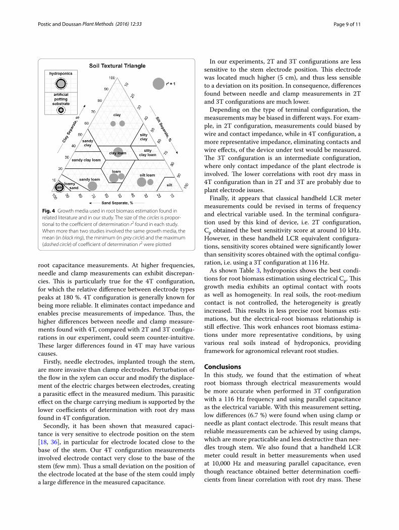
Page 9 of 11Postic and Doussan Plant Methods (2016) 12:33

root capacitance measurements. At higher frequencies, needle and clamp measurements can exhibit discrepan-cies. This is particularly true for the 4T configuration, for which the relative difference between electrode types peaks at 180 %. 4T configuration is generally known for being more reliable. It eliminates contact impedance and enables precise measurements of impedance. Thus, the higher differences between needle and clamp measure-ments found with 4T, compared with 2T and 3T configu-rations in our experiment, could seem counter-intuitive. These larger differences found in 4T may have various causes.

Firstly, needle electrodes, implanted trough the stem, are more invasive than clamp electrodes. Perturbation of the flow in the xylem can occur and modify the displace-ment of the electric charges between electrodes, creating a parasitic effect in the measured medium. This parasitic effect on the charge carrying medium is supported by the lower coefficients of determination with root dry mass found in 4T configuration.

Secondly, it has been shown that measured capaci-tance is very sensitive to electrode position on the stem [18, 36], in particular for electrode located close to the base of the stem. Our 4T configuration measurements involved electrode contact very close to the base of the stem (few mm). Thus a small deviation on the position of the electrode located at the base of the stem could imply a large difference in the measured capacitance.

In our experiments, 2T and 3T configurations are less sensitive to the stem electrode position. This electrode was located much higher (5  cm), and thus less sensible to a deviation on its position. In consequence, differences found between needle and clamp measurements in 2T and 3T configurations are much lower.

Depending on the type of terminal configuration, the measurements may be biased in different ways. For exam-ple, in 2T configuration, measurements could biased by wire and contact impedance, while in 4T configuration, a more representative impedance, eliminating contacts and wire effects, of the device under test would be measured. The 3T configuration is an intermediate configuration, where only contact impedance of the plant electrode is involved. The lower correlations with root dry mass in 4T configuration than in 2T and 3T are probably due to plant electrode issues.

Finally, it appears that classical handheld LCR meter measurements could be revised in terms of frequency and electrical variable used. In the terminal configura-tion used by this kind of device, i.e. 2T configuration, Cp obtained the best sensitivity score at around 10 kHz. However, in these handheld LCR equivalent configura-tions, sensitivity scores obtained were significantly lower than sensitivity scores obtained with the optimal configu-ration, i.e. using a 3T configuration at 116 Hz.

As shown Table 3, hydroponics shows the best condi-tions for root biomass estimation using electrical Cp. This growth media exhibits an optimal contact with roots as well as homogeneity. In real soils, the root-medium contact is not controlled, the heterogeneity is greatly increased. This results in less precise root biomass esti-mations, but the electrical-root biomass relationship is still effective. This work enhances root biomass estima-tions under more representative conditions, by using various real soils instead of hydroponics, providing framework for agronomical relevant root studies.

ConclusionsIn this study, we found that the estimation of wheat root biomass through electrical measurements would be more accurate when performed in 3T configuration with a 116 Hz frequency and using parallel capacitance as the electrical variable. With this measurement setting, low differences (6.7 %) were found when using clamp or needle as plant contact electrode. This result means that reliable measurements can be achieved by using clamps, which are more practicable and less destructive than nee-dles trough stem. We also found that a handheld LCR meter could result in better measurements when used at 10,000  Hz and measuring parallel capacitance, even though reactance obtained better determination coeffi-cients from linear correlation with root dry mass. These

Fig. 4 Growth media used in root biomass estimation found in related literature and in our study. The size of the circles is propor-tional to the coefficient of determination r2 found in each study. When more than two studies involved the same growth media, the mean (in black ring), the minimum (in grey circle) and the maximum (dashed circle) of coefficient of determination r2 were plotted

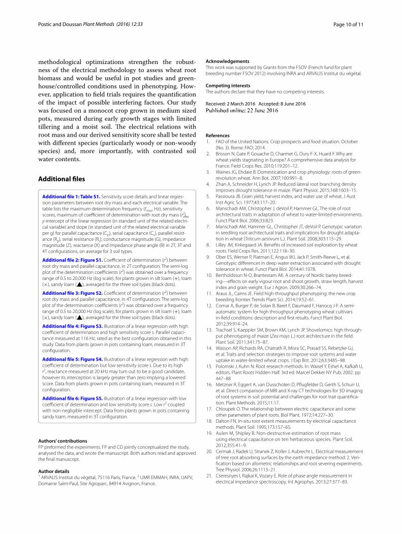
Page 10 of 11Postic and Doussan Plant Methods (2016) 12:33

methodological optimizations strengthen the robust-ness of the electrical methodology to assess wheat root biomass and would be useful in pot studies and green-house/controlled conditions used in phenotyping. How-ever, application to field trials requires the quantification of the impact of possible interfering factors. Our study was focused on a monocot crop grown in medium sized pots, measured during early growth stages with limited tillering and a moist soil. The electrical relations with root mass and our derived sensitivity score shall be tested with different species (particularly woody or non-woody species) and, more importantly, with contrasted soil water contents.

Authors’ contributionsFP preformed the experiments. FP and CD jointly conceptualized the study, analysed the data, and wrote the manuscript. Both authors read and approved the final manuscript.

Author details1 ARVALIS Institut du végétal, 75116 Paris, France. 2 UMR EMMAH, INRA, UAPV, Domaine Saint-Paul, Site Agroparc, 84914 Avignon, France.

Additional files

Additional file 1: Table S1. Sensitivity score details and linear regres-sion parameters between root dry mass and each electrical variable. The table lists the maximum determination frequency (fmax, Hz), sensitivity scores, maximum of coefficient of determination with root dry mass (rmax

2), y-intercept of the linear regression (in standard unit of the related electri-cal variable) and slope (in standard unit of the related electrical variable per g) for parallel capacitance (Cp), serial capacitance (Cs), parallel resist-ance (Rp), serial resistance (Rs), conductance magnitude (G), impedance magnitude (Z), reactance (X) and impedance phase angle (θ) in 2T, 3T and 4T configurations, on average for 3 soil types.

Additional file 2: Figure S1. Coefficient of determination (r2) between root dry mass and parallel capacitance, in 2T configuration. The semi-log plot of the determination coefficients (r2) was obtained over a frequency range of 0.5 to 20,000 Hz (log scale), for plants grown in silt loam (+), loam (×), sandy loam (▲), averaged for the three soil types (black dots).

Additional file 3: Figure S2. Coefficient of determination (r2) between root dry mass and parallel capacitance, in 4T configuration. The semi-log plot of the determination coefficients (r2) was obtained over a frequency range of 0.5 to 20,000 Hz (log scale), for plants grown in silt loam (+), loam (×), sandy loam (▲), averaged for the three soil types (black dots).

Additional file 4: Figure S3. Illustration of a linear regression with high coefficient of determination and high sensitivity score s. Parallel capaci-tance measured at 116 Hz, rated as the best configuration obtained in this study. Data from plants grown in pots containing loam, measured in 3T configuration.

Additional file 5: Figure S4. Illustration of a linear regression with high coefficient of determination but low sensitivity score s. Due to its high r2, reactance measured at 20 kHz may turn out to be a good candidate, however its interception is largely greater than zero implying a lowered score. Data from plants grown in pots containing loam, measured in 3T configuration.

Additional file 6: Figure S5. Illustration of a linear regression with low coefficient of determination and low sensitivity score s. Low r2 coupled with non-negligible intercept. Data from plants grown in pots containing sandy loam, measured in 3T configuration.

AcknowledgementsThis work was supported by Grants from the FSOV (French fund for plant breeding number FSOV 2012) involving INRA and ARVALIS Institut du végétal.

Competing interestsThe authors declare that they have no competing interests.

Received: 2 March 2016 Accepted: 8 June 2016

References 1. FAO of the United Nations. Crop prospects and food situation. October

(No. 3). Rome: FAO; 2014. 2. Brisson N, Gate P, Gouache D, Charmet G, Oury F-X, Huard F. Why are

wheat yields stagnating in Europe? A comprehensive data analysis for France. Field Crops Res. 2010;119:201–12.

3. Waines JG, Ehdaie B. Domestication and crop physiology: roots of green-revolution wheat. Ann Bot. 2007;100:991–8.

4. Zhan A, Schneider H, Lynch JP. Reduced lateral root branching density improves drought tolerance in maize. Plant Physiol. 2015;168:1603–15.

5. Passioura JB. Grain yield, harvest index, and water use of wheat. J Aust Inst Agric Sci. 1977;43:117–20.

6. Manschadi AM, Christopher J, deVoil P, Hammer GL. The role of root architectural traits in adaptation of wheat to water-limited environments. Funct Plant Biol. 2006;33:823.

7. Manschadi AM, Hammer GL, Christopher JT, deVoil P. Genotypic variation in seedling root architectural traits and implications for drought adapta-tion in wheat (Triticum aestivum L.). Plant Soil. 2008;303:115–29.

8. Lilley JM, Kirkegaard JA. Benefits of increased soil exploration by wheat roots. Field Crops Res. 2011;122:118–30.

9. Ober ES, Werner P, Flatman E, Angus WJ, Jack P, Smith-Reeve L, et al. Genotypic differences in deep water extraction associated with drought tolerance in wheat. Funct Plant Biol. 2014;41:1078.

10. Bertholdsson N-O, Brantestam AK. A century of Nordic barley breed-ing—effects on early vigour root and shoot growth, straw length, harvest index and grain weight. Eur J Agron. 2009;30:266–74.

11. Araus JL, Cairns JE. Field high-throughput phenotyping: the new crop breeding frontier. Trends Plant Sci. 2014;19:52–61.

12. Comar A, Burger P, de Solan B, Baret F, Daumard F, Hanocq J-F. A semi-automatic system for high throughput phenotyping wheat cultivars in-field conditions: description and first results. Funct Plant Biol. 2012;39:914–24.

13. Trachsel S, Kaeppler SM, Brown KM, Lynch JP. Shovelomics: high through-put phenotyping of maize (Zea mays L.) root architecture in the field. Plant Soil. 2011;341:75–87.

14. Wasson AP, Richards RA, Chatrath R, Misra SC, Prasad SS, Rebetzke GJ, et al. Traits and selection strategies to improve root systems and water uptake in water-limited wheat crops. J Exp Bot. 2012;63:3485–98.

15. Polomski J, Kuhn N. Root research methods. In: Waisel Y, Eshel A, Kafkafi U, editors. Plant Roots Hidden Half. 3rd ed. Marcel Dekker NY Pub; 2002. pp 447–88

16. Metzner R, Eggert A, van Dusschoten D, Pflugfelder D, Gerth S, Schurr U, et al. Direct comparison of MRI and X-ray CT technologies for 3D imaging of root systems in soil: potential and challenges for root trait quantifica-tion. Plant Methods. 2015;11:17.

17. Chloupek O. The relationship between electric capacitance and some other parameters of plant roots. Biol Plant. 1972;14:227–30.

18. Dalton FN. In-situ root extent measurements by electrical capacitance methods. Plant Soil. 1995;173:157–65.

19. Aulen M, Shipley B. Non-destructive estimation of root mass using electrical capacitance on ten herbaceous species. Plant Soil. 2012;355:41–9.

20. Cermak J, Radek U, Stranek Z, Koller J, Aubrecht L. Electrical measurement of tree root absorbing surfaces by the earth impedance method: 2. Veri-fication based on allometric relationships and root severing experiments. Tree Physiol. 2006;26:1113–21.

21. Cseresnyes I, Rajkai K, Vozary E. Role of phase angle measurement in electrical impedance spectroscopy. Int Agrophys. 2013;27:377–83.

Page 11 of 11Postic and Doussan Plant Methods (2016) 12:33

• We accept pre-submission inquiries

• Our selector tool helps you to find the most relevant journal

• We provide round the clock customer support

• Convenient online submission

• Thorough peer review

• Inclusion in PubMed and all major indexing services

• Maximum visibility for your research

Submit your manuscript atwww.biomedcentral.com/submit

Submit your next manuscript to BioMed Central and we will help you at every step:

22. Ellis T, Murray W, Kavalieris L. Electrical capacitance of bean (Vicia faba) root systems was related to tissue density—a test for the Dalton Model. Plant Soil. 2013;366:575–84.

23. Ozier-Lafontaine H, Bajazet T. Analysis of root growth by impedance spectroscopy (EIS). Plant Soil. 2005;277:299–313.

24. van Beem J, Smith ME, Zobel RW. Estimating root mass in maize using a portable capacitance meter. Agron J. 1998;90:566–70.

25. Dietrich RC, Bengough AG, Jones HG, White PJ. Can root electrical capaci-tance be used to predict root mass in soil? Ann Bot. 2013;112:457–64.

26. Dietrich RC, Bengough AG, Jones HG, White PJ. A new physical interpreta-tion of plant root capacitance. J Exp Bot. 2012;63:6149–59.

27. Nakhforoosh A, Grausgruber H, Kaul H-P, Bodner G. Wheat root diversity and root functional characterization. Plant Soil. 2014;380:211–29.

28. Heřmanská A, Středa T, Chloupek O. Improved wheat grain yield by a new method of root selection. Agron Sustain Dev. 2015;35:195–202.

29. Liao A, Zhou Q, Zhang Y. Application of 3D electrical capacitance tomography in probing anomalous blocks in water. J Appl Geophys. 2015;117:91–103.

30. Samouëlian A, Cousin I, Tabbagh A, Bruand A, Richard G. Electrical resistiv-ity survey in soil science: a review. Soil Tillage Res. 2005;83:173–93.

31. Nyce DS. Linear position sensors: theory and application. Hoboken: Wiley-Interscience; 2004.

32. Kendall WA, Pederson GA, Hill RR. Root size estimates of red clover and alfalfa based on electrical capacitance and root diameter measurements. Grass Forage Sci. 1982;37:253–6.

33. Zanetti C, Weller A, Vennetier M, Meriaux P. Detection of buried tree root samples by using geoelectrical measurements: a laboratory experiment. Plant Soil. 2011;339:273–83.

34. Cao Y, Repo T, Silvennoinen R, Lehto T, Pelkonen P. Analysis of the willow root system by electrical impedance spectroscopy. J Exp Bot. 2011;62:351–8.

35. Chloupek O, Dostál V, Středa T, Psota V, Dvořáčková O. Drought toler-ance of barley varieties in relation to their root system size. Plant Breed. 2010;129:630–6.

36. Ellis TW, Murray W, Paul K, Kavalieris L, Brophy J, Williams C, et al. Electrical capacitance as a rapid and non-invasive indicator of root length. Tree Physiol. 2013;33:3–17.

37. Chloupek O. Evaluation of the size of a plant’s root system using its elec-trical capacitance. Plant Soil. 1977;48:525–32

68

 

Chapitre 2

69

Chapitre 2 : Impact des systèmes racinaires de

différentes variétés de blé en conditions multi-

stressantes, mis en évidence à l’aide de

minirhizotrons à scanner

François Postic Katia Beauchêne David Gouache 

Guillaume Meloux Claude Doussan 

   

    

Chapitre 2

70

Ce deuxième chapitre s'intéresse à l’apport des minirhizotrons dans le cadre de comparaisons

variétales pour des cultures de blé, en ce qui concerne la dynamique racinaire et la

compréhension des variations de réactions face à des stress hydriques et/ou azotés. Les

minirhizotrons modernes ont rarement été utilisés pour grande cultures, et ainsi, un essai

agronomique a été mis en place à Gréoux-les-Bains en 2013–2014 et 2014–2015 sur 4

variétés de blé contrastées — comprenant un blé tendre, un blé dur, un blé synthétique et un

blé hybride — cultivés sous 4 traitements différents (combinaison entre présence et absence

de stress hydrique ou de stress azoté). La profondeur de sol de l’essai varie selon les

situations, la zone irriguée et faiblement fertilisée ayant une faible profondeur de sol (cf.

Figure S1 en annexe du chapitre 2).

Les résultats montrent que les minirhizotrons donnent des estimations biaisées de la masse

racinaire superficielle (0–40 cm), mais semblent fiables pour les parties du système racinaire

plus profondes (>40 cm). De plus, en conditions pluviales, les rendements obtenus sont

positivement corrélés à la quantité de racines mesurée en profondeur.

Ce chapitre est un manuscrit formaté pour une pré-soumission qui suit les exigence du journal

scientifique visé. Cet article a été soumis à Field Crop Research, qui demande d’intégrer une

deuxième année d’expérimentation agronomique.

71 

Scanner-based minirhizotrons evidenced the impact of root

systems in various wheat cultivars under multi-stressed conditions

François Postic1,2,*, Katia Beauchêne1, David Gouache1, Guillaume Meloux1 and Claude

Doussan2

1ARVALIS Institut du végétal, 3 rue Joseph et Marie Hackin, 75116 Paris, France.

2UMR EMMAH, INRA, UAPV, Domaine Saint-Paul, Site Agroparc, 84914 Avignon, France.

* Corresponding author: francois.postic@paca.inra.fr

Chapitre 2

72

Abstract

Adapting crops to climate change would greatly benefit breeding programs that can rely on

root phenotyping tools in field conditions—and this particularly applies to wheat crops. Such

in-field phenotyping necessitates the development of rapid and non-destructive measurement

techniques for the screening of relevant root traits under sub-optimal conditions. In this study,

we used scanner-based minirhizotrons to measure in situ the root length and volume densities

of 4 wheat varieties, under 4 different growth conditions: irrigated and rainfed conditions

coupled with optimal and sub-optimal N fertilization under a Mediterranean climate. These

measurements were performed at 4 growth stages. For all the treatments, grain yield correlates

with minirhizotron-based root surface density measured at anthesis (r2 = 0.48). Irrigated and

rainfed conditions led to contrasted relations between roots and grain yield: no correlation was

found in irrigated plots, even if under rainfed conditions and sub-optimal fertilization, the

higher yields were related to a higher root colonization of the deep soil layers (r2 = 0.40).

Shoot biomass was correlated to grain yield in irrigated conditions, but not in rainfed

conditions. However, for the latter, the total root weight, the proportion of which being

mainly located in the shallow soil layers, is not related to grain yield. We propose that high

grain yield under stress condition are attained by a stress avoidance mechanism of the root

system characterised by a higher root density in the deep soil layers. Thus, unlike shoot

biomass measurements, scanner-based minirhizotron provides a essential tool to detect wheat

genotypes with superior stress avoidance capability.

Keywords

Wheat, root, minirhizotron, drought resistance, nitrogen stress

Chapitre 2

73

Abbreviations

DOF – Depth of field Centimetres, cm

GY – Grain yield Tons per hectares, t.ha-1

Mh1 – Mean root mass of 10–20 cm samples from the central row Grams per metres squared, g.m-2

Mh2 – Mean root mass of 30–40 cm samples from the central row, g.m-2

Mh2i – Mean root mass of 30–40 cm samples from the inter-row, g.m-2

RDM – Total root dry mass density (auger and minirhizotron Tons per hectares, t.ha-1

RDMa – Root dry mass density from auger sampling Grams per metres squared, g.m-2

RDMm –Root dry mass density from minirhizotron data Grams per metres squared, g.m-2

RLD – Root length density Millimetres per centimetres squared, mm.cm-2

RLSD – Root surface length density, mm.cm-2

R:S – Root to shoot ratio Dimensionless

SDM – Shoot dry mass Tons per hectares, t.ha-1

SRL – Specific root length Metres per grams, m.g-1

TRLSD – Total root length surface density, mm.cm-2

μ1/2 – Median of the equivalent sampling thickness of minirhizotrons, m

ε – Equivalent sampling thickness of minirhizotrons, m

Chapitre 2

74

1. Introduction

Driven by a growing world population, cereal demand and production is predicted to increase

by 30 to 50 % in 2050 relative to 2005 (Tilman et al., 2011; Alexandratos and Bruinsma,

2012). Most of this increase is expected to come from an increase in yield and mostly from

genetic improvement (Reynolds et al., 2000; Langridge, 2005; Alexandratos and Bruinsma,

2012). However, climate change associated with increased uncertainty and variability in

precipitations and increase of temperature challenges yield improvement. It is already the case

in top producers of western Europe such as France where climate change, coupled with

changes in agronomic policies, is identified in the contribution to wheat yield stagnation since

1995-1998 (Brisson et al., 2010). Among climatic factors, spring droughts and high

temperatures are the main abiotic stress that limits winter cereal crop productions. South and

coastal regions of Europe could face a dramatic yield decrease caused by droughts during

grain filling period, highly variable precipitation during spring and high temperatures during

late spring (Iglesias et al., 2012).

Concomitantly to climate change, intensive agricultural production is also faced to

sustainability issues with increasing pressures on water resource and availability of fertilizers

as well as environmental negative impacts.

More stressing conditions may impact large area in the future and there is a need to determine

crop plant traits that would improve or maintain the yield. Historically, improvement of crops

and agricultural techniques targeted on increasing shoot biomass and grain yield, while

overlooking the root system in crop production. However, the root system ensures crucial

functions, such as water and nutrient uptakes, and its role is determinant under limiting low

inputs conditions (Waines and Ehdaie, 2007; Herder et al., 2010). The roots traits associated

Chapitre 2

75

in the efficient use of available water and fertilizers by crops, in possible variable deficit

conditions, would be an important feature in the selection of the future phenotypes.

In relation with drought resistance, the roots traits can be identified at the vegetative or

reproductive stages and defined from either local or global root system architecture (RSA)

characteristics.

Crops differ in root system architecture and in water capture ability. A study showed that a

straightforward factor that fit the whole root distribution is related to the efficiency in

recovering water (Monti and Zatta, 2009). For example, the miscanthus concentred top layers

roots confer a higher efficiency in water use than sorghum, which root system is deeper.

In contrast, specific local traits, often measured on seedlings, such as the root angle can be

also related to drought resistance, in generating a variable pattern of horizontal relative to

vertical exploration of soil by roots (Manschadi et al., 2008).

With the aim of identifying heritability and genetic determinants of root traits, mainly at

relatively young stages, different types of root observation facilities have been developed in

relation with high-throughput phenotyping requirements for modern breeding programs. Pot

based experiment at the laboratory scale allow a high control of environmental conditions and

repeatability with detailed investigations of the root systems through imaging techniques such

as rhizoponics (Mathieu et al., 2015), X-ray tomography (Mooney et al., 2012), magnetic

resonance imaging (Metzner et al., 2015) or the growth and luminescence observatory

(Rellán-Álvarez et al., 2015). However, a major disadvantage of these techniques is that the

container size has an effect on growth and the root phenes. On a greater spatial scale, but at

the cost of development of heavy subterranean facilities, rhizolysimeters allow experiments

with larger containers size that can be heavily equipped to monitor soil parameters and root

development estimated with minirhizotron (Eberbach et al., 2013).

Chapitre 2

76

However, in situ root development and functioning result from the expression of a myriad of

genes triggered by interactions between the plant genome and the environment. Resulting

from this G×E interaction, the screening of wheat root traits under controlled environment has

been shown not always representative for field conditions (Watt et al., 2013), which makes

the genetic or molecular identification of beneficial root traits challenging for plant breeders.

Field and soil environments are biologically, physically and chemically heterogeneous, that

alter root growth response trough plasticity of the root system. That is the case for the

distribution of nutrients in the soil which affects the root distribution and, for example,

shallow- or deep-distribution of nitrogen induces shallow- or deep-root systems (Sharma and

Chaudhary, 1983).

Moreover, the interaction of multiple abiotic stresses in relation with roots functioning and

development is rarely examined, particularly in the field, and most of the literature focuses on

interaction involving temperature (Rich and Watt, 2013). For wheat, studies conducted under

field and near-field conditions show that a water deficit induces a deeper rooting (Barraclough

et al., 1991). A low nitrogen fertilization can also induce a higher proportion of deep roots,

especially when water table at seeding time is low (Kmoch et al., 1957), while nitrogen

fertilization increased the total root length by 30% (Barraclough et al., 1991). Nonetheless,

the combination of these two stresses—drought and nitrogen deficit—results in an overall

lower root densities over the soil profile (Barraclough et al., 1989; Herrera et al., 2007).

Field-studies combine multiple interactions, with most of the soil environment being beyond

control and a limited access to the quantification of occurring factors. Despite a lower control

on growth conditions, such field-based studies are needed for identifying relevant root traits

and are a necessary step for understanding the root system response to various soil conditions.

Their major disadvantages lie in that they are labour and time expensive, mostly destructive,

and affected by soil heterogeneity. For root quantification, soil coring, shovelomics (Trachsel

Chapitre 2

77

et al., 2011), and minirhizotrons (Maeght et al., 2013) are the main techniques used. Beyond

of their actual time-consumption, field sampling methods remain destructives, and can lead to

oversized experimental installations (Polomski et al., 2002).

Among existing sampling methods, minirhizotrons—an invasive, but not destructive

techniques—allow the dynamic study of several root traits. This technique consists in

observing roots in situ through a transparent tube inserted in the soil. Most minirhizotron

applications used video recorders (BTX-100, Bartz Technology Company, Santa Barbara,

CA, USA) capturing images of small surface area (4 cm²), which made the recording of a

whole tube time-expensive and exposed to positional errors. As a recent technology,

minirhizotrons can be now be imaged by a rotary scanner that captures 400 cm² images (CI-

600, CID Bio-Science, Camas, WA, USA), so that the complete surface of a 20 cm long tube,

with a 7 cm diameter, is obtained within a single scan. This better practicability could lead to

an increase in the number of available observational data about plant roots. However, most

root image processing softwares are not designed for images featuring a soil background, as

found in the images from minirhizotrons. For example, beyond reported biases (Wang and

Zhang, 2009), WhinRhizo—the most widely used software—features an automatic root

detection conceived for white background images. Nevertheless, once roots are identified on

the images, minirhizotrons allow rapid assessment of root diameter and root length, and thus,

require less labour and time than other field-based techniques, particularly for deep root

observation.

Minirhizotron studies based on this kind of large images obtain with a rotary scanner are few

in the field of crop research. A rotary scanner minirhizotron was used in a prior study for

evaluating the influence of tillage on wheat root system (Munoz-Romero et al., 2010). With

this technique, the authors obtained root data that successfully explained the higher rainfed

Chapitre 2

78

wheat productivity under no-tillage. However, to our knowledge, rotary scanner minirhizotron

has not been yet employed to measure root systems of crops under nutrient- or water-stress

conditions and the potential of this minirhizotron technique to screen for root characteristics

remains unknown.

In this study, we propose to i) test a methodology to convert root length observed with

minirhizotron into root mass found with standard auger sampling, ii) evaluate the root data in

regard of the dynamics of physiological traits, iii) to examine the relevance of such

minirhizotron measures of roots in multi-stress trial for various wheat cultivar.

2. Material and Methods

2.1. Localization of experiments

Field experiments were conducted in Gréoux-les-Bains, south-east France (43°7478 N,

5°8519E), on a heterogeneous Fluviosol with a silt Loam texture (Figure 1a). Located in the

Mediterranean climatic region, the mean annual rainfall over the last 20 years is 650.3 mm

(distributed as 32% in October–December; 18% in January–March; 28% in April–June; and

22% for July–September); the average annual potential evapotranspiration (PET) is 955.5

mm; and for temperature: mean annual temperature 12.68°C; average temperature of the

coldest month 4.5°C; average temperature of the warmest month 21.8°C. The weather and

temperature data (Figure 2) were obtained from a meteorological station located 700 m from

the experimental plots. During the growth of winter wheat crop, sowing on 28th October 2014

and harvest on 01st July 2015, the cumulated rainfall was 539.7 mm while PET was 553.0

mm. The preceding crop on the trial site what durum wheat.

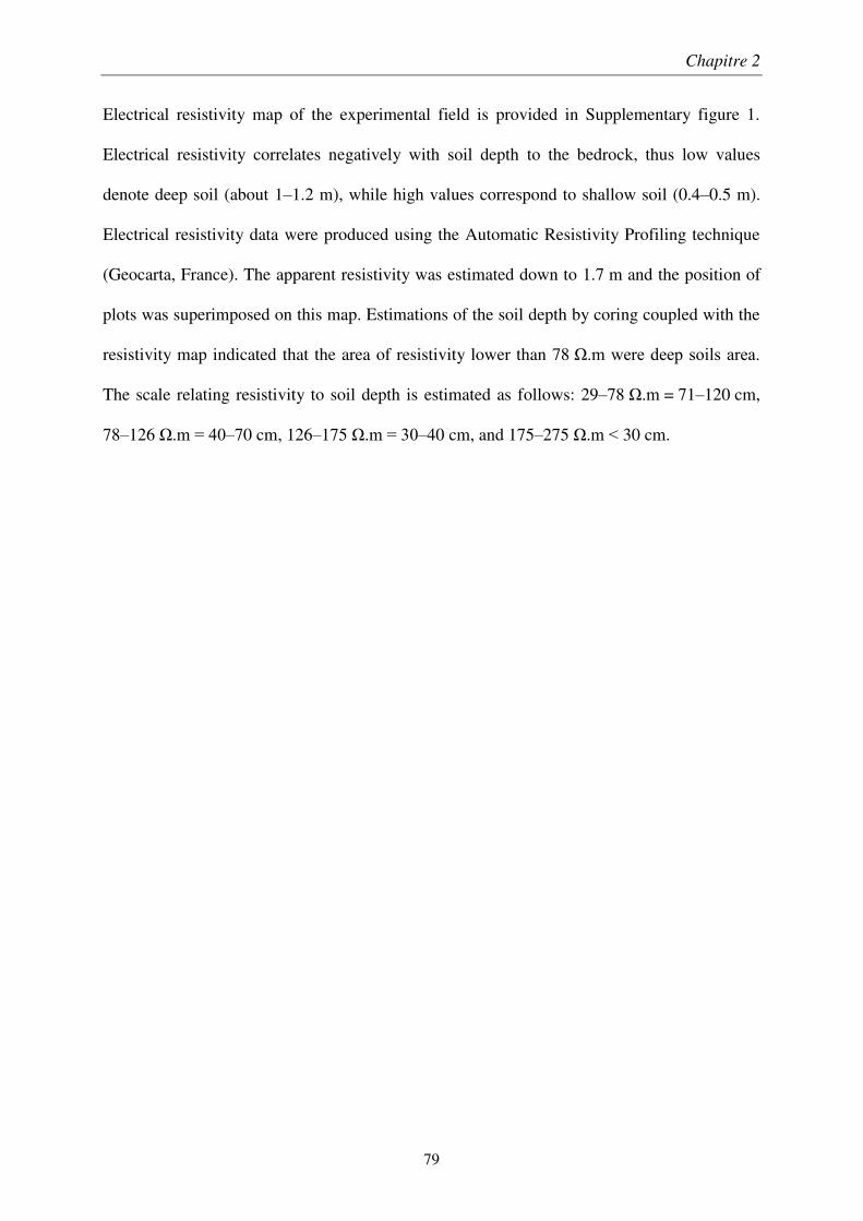
Chapitre 2

79

Electrical resistivity map of the experimental field is provided in Supplementary figure 1.

Electrical resistivity correlates negatively with soil depth to the bedrock, thus low values

denote deep soil (about 1–1.2 m), while high values correspond to shallow soil (0.4–0.5 m).

Electrical resistivity data were produced using the Automatic Resistivity Profiling technique

(Geocarta, France). The apparent resistivity was estimated down to 1.7 m and the position of

plots was superimposed on this map. Estimations of the soil depth by coring coupled with the

resistivity map indicated that the area of resistivity lower than 78 Ω.m were deep soils area.

The scale relating resistivity to soil depth is estimated as follows: 29–78 Ω.m = 71–120 cm,

78–126 Ω.m = 40–70 cm, 126–175 Ω.m = 30–40 cm, and 175–275 Ω.m < 30 cm.

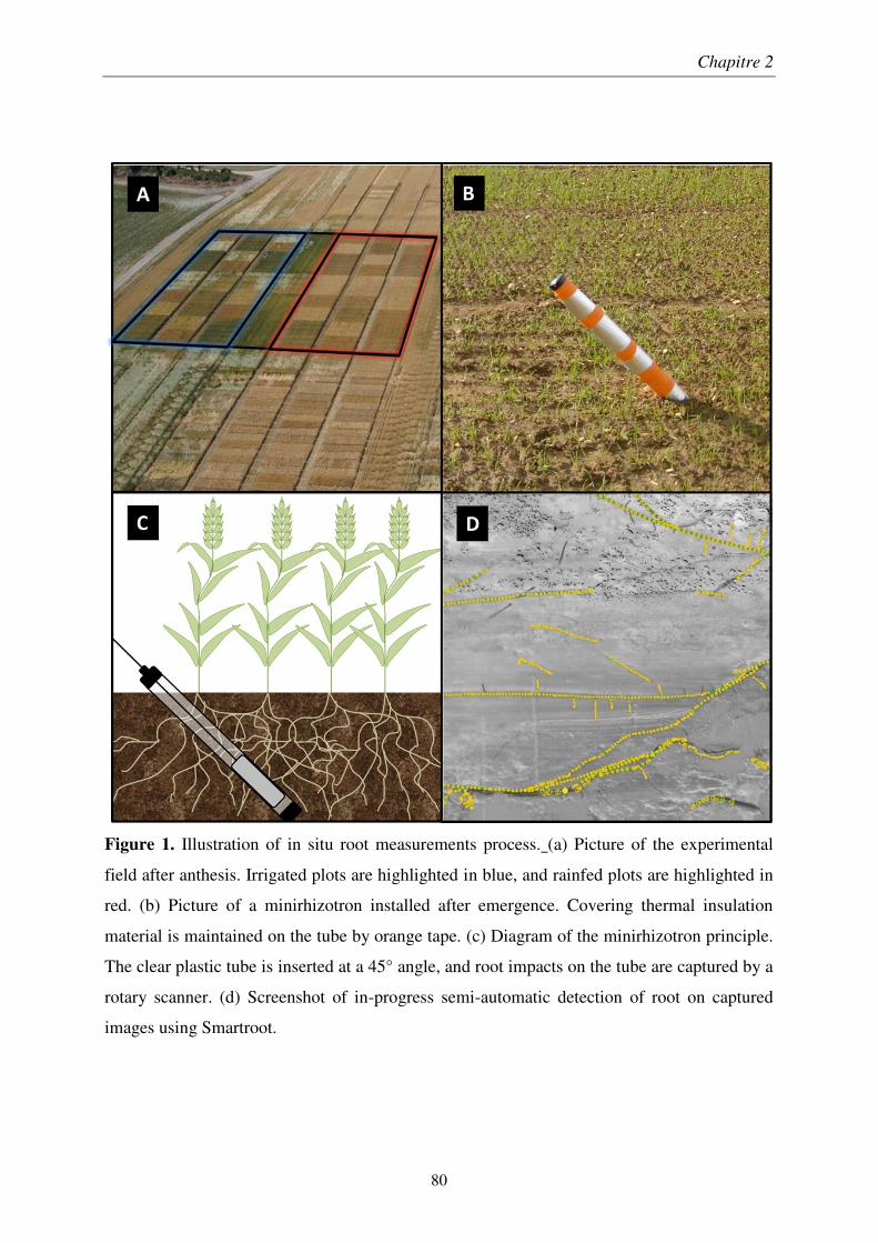
Chapitre 2

80

Figure 1. Illustration of in situ root measurements process. (a) Picture of the experimental

field after anthesis. Irrigated plots are highlighted in blue, and rainfed plots are highlighted in

red. (b) Picture of a minirhizotron installed after emergence. Covering thermal insulation

material is maintained on the tube by orange tape. (c) Diagram of the minirhizotron principle.

The clear plastic tube is inserted at a 45° angle, and root impacts on the tube are captured by a

rotary scanner. (d) Screenshot of in-progress semi-automatic detection of root on captured

images using Smartroot. 

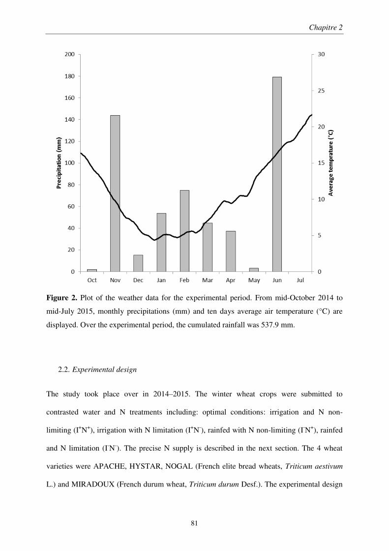
Chapitre 2

81

Figure 2. Plot of the weather data for the experimental period. From mid-October 2014 to

mid-July 2015, monthly precipitations (mm) and ten days average air temperature (°C) are

displayed. Over the experimental period, the cumulated rainfall was 537.9 mm. 

2.2. Experimental design

The study took place over in 2014–2015. The winter wheat crops were submitted to

contrasted water and N treatments including: optimal conditions: irrigation and N non-

limiting (I+N+), irrigation with N limitation (I+N-), rainfed with N non-limiting (I-N+), rainfed

and N limitation (I-N-). The precise N supply is described in the next section. The 4 wheat

varieties were APACHE, HYSTAR, NOGAL (French elite bread wheats, Triticum aestivum

L.) and MIRADOUX (French durum wheat, Triticum durum Desf.). The experimental design

Chapitre 2

82

was a randomized complete block with three replications. The area of each experimental plot

was 9.5 × 6.6 m².

2.3. Crop management

Wheat cultivars were sown in late October 2014 after ploughing (25 cm), and preparing the

seed bed by disc harrowing and tilling with a vibrating tine cultivator. The four varieties were

planted in 17.5 cm inter-rows at 300 grains per m². During the wheat growing season, weed

control was performed by aspersing four herbicides three times and fungicides were applied

twice at flag leaf ligule and anthesis. Irrigation was applied on I+N+ and I+N-, six times

totalizing 189 mm, while the rainfed plots received no irrigation. Nitrogen fertilizer

application rates were designed accounting the differences in yield potential under drought

conditions. Nitrogen fertilizer was applied at four different rates: I+N+ (230 kg.ha-1, four

applications); I+N-, (100 kg.ha-1, two applications); I-N+ (150 kg ha-1 three applications) and I-

N- (50 kg ha-1, one application).

2.4. Shoot biomass and N measurements

Variations in shoot dry mass and nitrogen content of plants were determined at different

growth stages. The growth stages of wheat were estimated using the Zadoks scale (Zadoks et

al., 1974) and destructive plant measurements were done at two unfolded leaf (Z12), stem

elongation (Z30), flag leaf ligule (Z39), anthesis half-way (Z65) and ripening (Z91). Shoot

biomass was sampled from a 0.70 m² area in each plot. Fresh and dry shoot mass were

measured on an electronic scale and dry biomass was obtained by oven-drying at 80°C for

48h. Nitrogen content of shoot was performed by collecting two samples of plant material

Chapitre 2

83

from the 0.7 m² area. The level of nitrogen deficit was calculated with the nitrogen nutrition

index (NNI, in %) for winter wheat (Justes et al., 1994). The wheat grain yield (GY15, in t.ha-

1) was determined on 9.5 × 1.225 m² by using a combine harvester (ZURN 150).

2.5. Root measurements

2.5.1. Minirhizotron installation

Root imaging from minirhizotrons was performed with the CI-600 root scanner (CID Bio-

Science, Camas, WA, USA), controlled by a laptop computer. The size of the recorded

images was 21.59 cm × 19.56 cm, with a 300-dpi resolution (Figure 1d). Minirhizotron tubes

were clear acrylic glass (PMMA) tubes of 2.0 m length, 6.3 cm inner diameter and 7.0 cm

outer diameter. Minirhizotron tubes were inserted into the central sowing line of each plot,

with a 45° angle, after plant emergence (Figure 1b). Soil drilling for tube installation was

performed using a 7  cm diameter auger and a self-made 45° drilling frame. Tubes were

inserted to a maximum vertical depth of 122 cm, depending on the gravel depth. The above-

ground part of each tube was covered with thermal insulation foils, to prevent light,

condensation and sun warming of the tube. Images were captured at tillering (Z25), stem

elongation (Z30), flag leaf ligule (Z39) and anthesis half-way (Z65).

2.5.2. Image processing of minirhizotron images

The images were processed using the Smartroot software (Lobet et al., 2011): root length and

root diameter were measured on every image (Figure 1d). Root length surface density along

the tube (TRLSD, in mm.cm-2) was computed for each tube, according to their actual length

over the tube surface area. The mean root length surface density profiles, for each wheat

Chapitre 2

84

variety and treatment, were obtained by averaging replicate RLSD profiles. Before averaging

RLSD profiles, an interpolation was performed using a cubic Hermite spline in order to get

the RLSD values at the same depths.

2.5.3. Auger sampling for root biomass

An auger (40 mm diameter) was used to collect two soil samples in the central row of each

plot, and a third soil sample in the middle of the nearby inter-row at tillering (Z25), stem

elongation (Z30), flag leaf ligule (Z39) and anthesis half-way (Z65). Central rows were

sampled at 10–20 cm and 30–40 cm depth, and inter-rows were sampled at 30–40 cm. Roots

were washed from the soil for 10 min using a hydropneumatic elutriator, collected on 350 µm

sieves, ovendried at 70°C for 48h, and then weighted.

For each plot, the total root biomass from the surface to 40 cm depth was calculated by

assuming biomass at 10–20 cm depth equals biomass from 0–10 cm and with linear

interpolation of root biomass at 20–30 cm depth. The root dry mass density over 0–40 cm

depth (𝑅𝐷𝑀𝑎, g.m-2) is estimated by:

𝑅𝐷𝑀𝑎 = 2 × 𝑀ℎ1 +𝑀ℎ2 + 𝑀ℎ2𝑖 + 2 × 𝑀ℎ1

4+

𝑀ℎ2 + 𝑀ℎ2𝑖

2 (Eq. 1)

Where 𝑀ℎ1 is the mean root biomass (g.m-2) of 10–20 cm samples from the central row, 𝑀ℎ2

is the mean root biomass (g.m-2) of 30–40 cm samples from the central row, 𝑀ℎ2𝑖 is the mean

root biomass (g.m-2) of 30–40 cm samples from the inter-row.

2.5.4. Conversion of root length surface density to root biomass

Chapitre 2

85

For converting root length surface density data from images to root biomass, we assumed that

the soil volume sampled by the minirhizotron is a cylindrical shell. The inner radius of the

shell is the tube outer radius and its thickness (ε) is the image depth of field of view of the

scanner (Figure 3). This assumption implies that the root density measured in this soil volume

sampled by the minirhizotron is the same as the root density measured in an extracted soil

core.

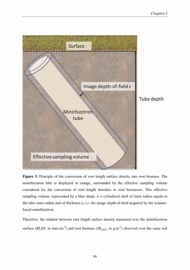
Chapitre 2

86

Figure 3. Principle of the conversion of root length surface density into root biomass. The

minirhizotron tube is displayed in orange, surrounded by the effective sampling volume

considered for the conversion of root length densities to root biomasses. This effective

sampling volume, represented by a blue shade, is a cylindrical shell of inner radius equals to

the tube outer radius and of thickness ε, i.e. the image depth-of-field acquired by the scanner-

based minirhizotron.

Therefore, the relation between root length surface density measured over the minirhizotron

surface (RLSD, in mm.cm-2) and root biomass (𝑀𝑟𝑜𝑜𝑡, in g.m-2) observed over the same soil

Chapitre 2

87

thickness (Δ𝑧, in m) for coring and minirhizotron tube, inserted into the soil at a specific angle

(𝜑, in radian) is given by:

𝑀𝑟𝑜𝑜𝑡 =𝑅𝐿𝑆𝐷

𝜀 × 𝑆𝑅𝐿× Δ𝑧 × cos(𝜑) (Eq. 2)

Where SRL denotes the specific root length (m.g-1). The values of the product ε × SRL—the

conversion factor of root length into root mass—were obtained by using minirhizotron and

soil sampling data of samples from soil layer at 30–40 cm depth. The median (μ1/2) value of

the product ε × SRL is calculated using the mean specific root length observed in situ for

winter wheat crops, i.e. SRL = 180 m.g-1 (Løes and Gahoonia, 2004).

Alternative approaches for converting root length surface density obtained by minirhizotron

into equivalent cored values exist. A similar method of calibration used a zero intercept linear

regression (Zhang et al., 2008), instead of the distribution of conversion factors, while other

approaches rely on on the maximum diameter of observed roots as DOF (Atkinson, 1985).

2.6. Root to shoot ratio

The root to shoot ratio (R:S) was calculated at tillering (Z25), stem elongation (Z30), flag leaf

ligule (Z39) and anthesis half-way (Z65) as the ratio between the total root dry mass (RDM,

in t.ha-1) and the shoot dry mass (SDM, in t.ha-1). The total root mass was computed as the

sum of the root biomass estimations by auger sampling (RDMa, in g.m-2), and the

minirhizotron root length measurements converted into root biomass (RDMm, in g.m-2) (Eq

3). In order to prevent overlap of root data, only measurements of root length via

minirhizotron deeper than 40 cm were considered.

𝑅𝐷𝑀 = 𝑅𝑀𝐷𝑎 + 𝑅𝐷𝑀𝑚|𝑧 > 40𝑐𝑚 (Eq. 3)

Chapitre 2

88

2.7. Statistical analyses

An analysis of variance (ANOVA) with a mixed linear effect model of grain yield (GY15),

shoot dry mass (SDM) and root dry mass (RDM) was calculated using MATLAB. Genotype

(G), nitrogen treatment (N) and irrigation treatment (I) were considered as fixed effect, and

replicates were considered as random effect. The means of the minirhizotrons depth (due to

soil depth variations) were compared using the Fischer’s least significant difference test at

0.05 probability level. The correlations between the different root and shoot variables were

computed with MATLAB, along with p-values of the slope of the regression line. Coefficient

of determination values (r2) were calculated using the squared Pearson product-moment

correlation coefficient.

The α < 0.05 confidence band for the median of the conversion factor (μ1/2) for RLSD to

biomass (𝜀 × 𝑆𝑅𝐿) and for the mean of the root to shoot ratio (R:S) at the four growth stages,

namely tillering (Z25), stem elongation (Z30), flag leaf ligule (Z39) and anthesis half-way

(Z65), were computed using a non-parametric bootstrap with 100,000 paired sampled, drawn

from the experimental pairs with replacement. The α/2 and 1-α/2 quantiles of the bootstrapped

distribution of μ1/2 and of R:S were considered for the limits of the confidence interval.

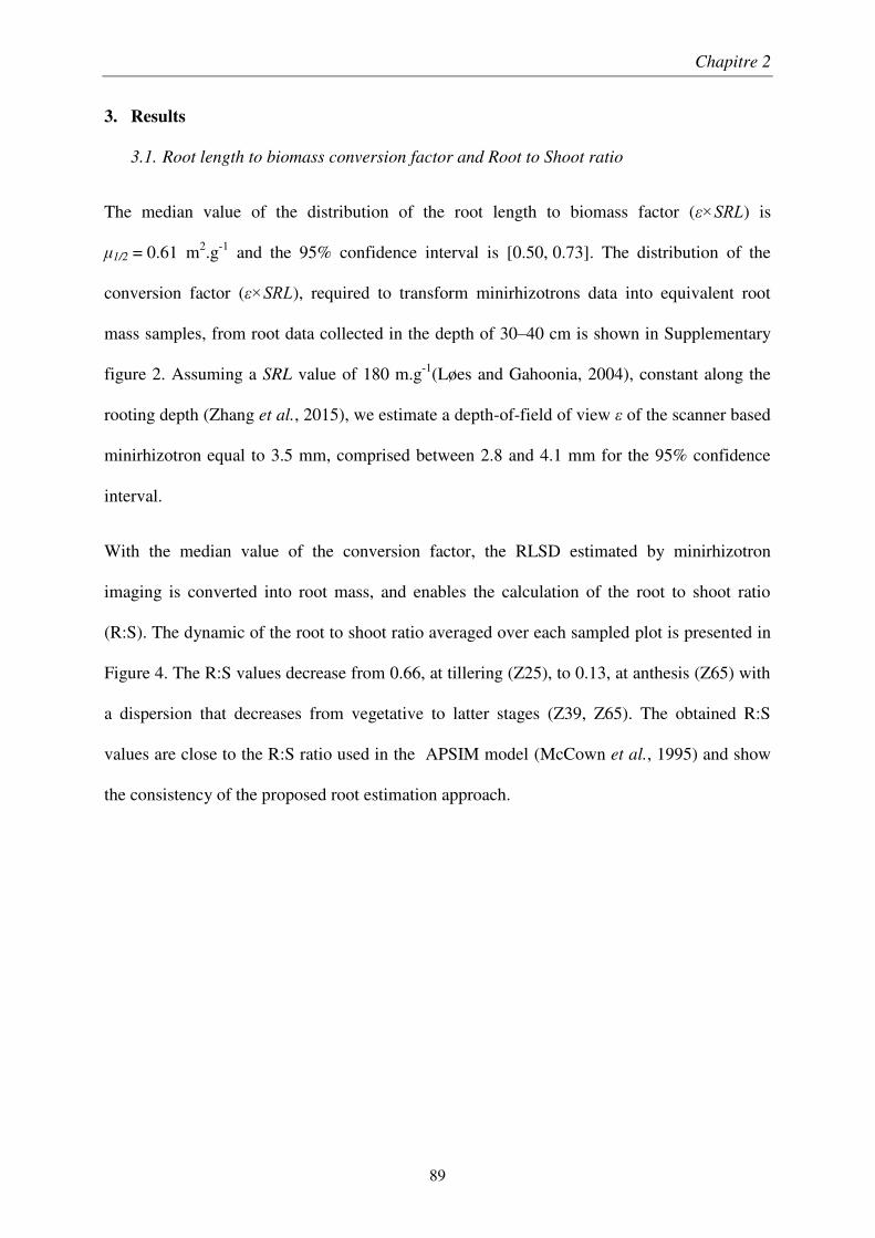
Chapitre 2

89

3. Results

3.1. Root length to biomass conversion factor and Root to Shoot ratio

The median value of the distribution of the root length to biomass factor (ε×SRL) is

μ1/2 = 0.61 m2.g-1 and the 95% confidence interval is [0.50, 0.73]. The distribution of the

conversion factor (ε×SRL), required to transform minirhizotrons data into equivalent root

mass samples, from root data collected in the depth of 30–40 cm is shown in Supplementary

figure 2. Assuming a SRL value of 180 m.g-1(Løes and Gahoonia, 2004), constant along the

rooting depth (Zhang et al., 2015), we estimate a depth-of-field of view ε of the scanner based

minirhizotron equal to 3.5 mm, comprised between 2.8 and 4.1 mm for the 95% confidence

interval.

With the median value of the conversion factor, the RLSD estimated by minirhizotron

imaging is converted into root mass, and enables the calculation of the root to shoot ratio

(R:S). The dynamic of the root to shoot ratio averaged over each sampled plot is presented in

Figure 4. The R:S values decrease from 0.66, at tillering (Z25), to 0.13, at anthesis (Z65) with

a dispersion that decreases from vegetative to latter stages (Z39, Z65). The obtained R:S

values are close to the R:S ratio used in the APSIM model (McCown et al., 1995) and show

the consistency of the proposed root estimation approach.

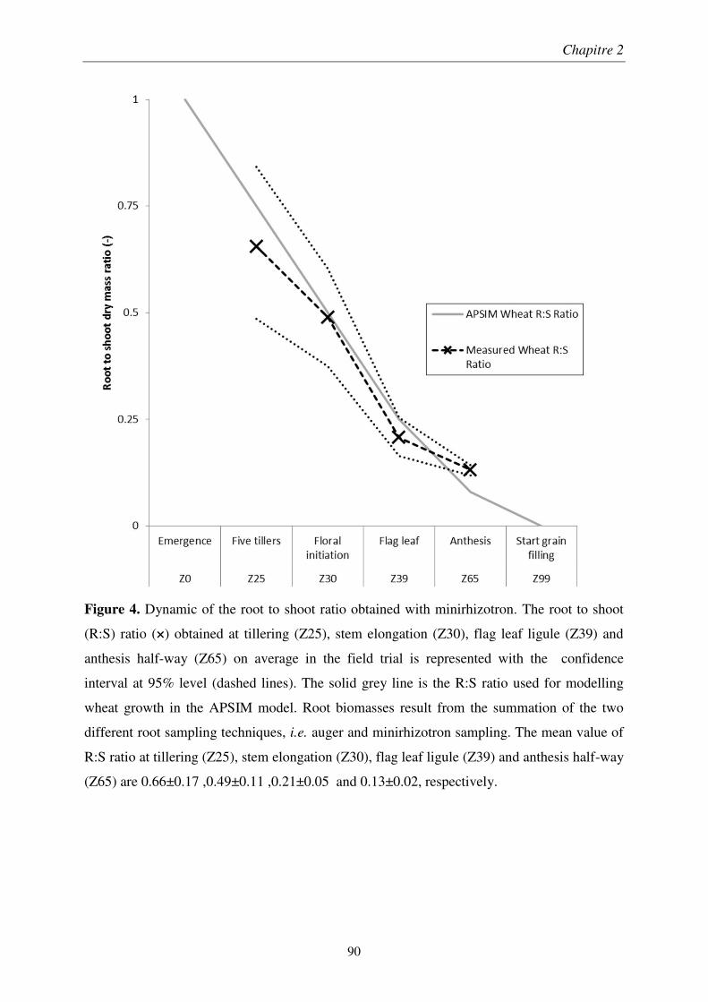
Chapitre 2

90

Figure 4. Dynamic of the root to shoot ratio obtained with minirhizotron. The root to shoot

(R:S) ratio (×) obtained at tillering (Z25), stem elongation (Z30), flag leaf ligule (Z39) and

anthesis half-way (Z65) on average in the field trial is represented with the confidence

interval at 95% level (dashed lines). The solid grey line is the R:S ratio used for modelling

wheat growth in the APSIM model. Root biomasses result from the summation of the two

different root sampling techniques, i.e. auger and minirhizotron sampling. The mean value of

R:S ratio at tillering (Z25), stem elongation (Z30), flag leaf ligule (Z39) and anthesis half-way

(Z65) are 0.66±0.17 ,0.49±0.11 ,0.21±0.05 and 0.13±0.02, respectively.

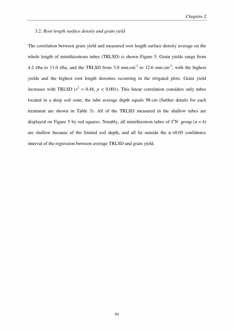
Chapitre 2

91

3.2. Root length surface density and grain yield

The correlation between grain yield and measured root length surface density average on the

whole length of minirhizotrons tubes (TRLSD) is shown Figure 5. Grain yields range from

4.2 t/ha to 11.0 t/ha, and the TRLSD from 3.0 mm.cm-2 to 12.6 mm.cm-2, with the highest

yields and the highest root length densities occurring in the irrigated plots. Grain yield

increases with TRLSD (r2 = 0.48, p < 0.001). This linear correlation considers only tubes

located in a deep soil zone, the tube average depth equals 98 cm (further details for each

treatment are shown in Table 3). All of the TRLSD measured in the shallow tubes are

displayed on Figure 5 by red squares. Notably, all minirhizotron tubes of I+N- group (n = 4)

are shallow because of the limited soil depth, and all lie outside the α <0.05 confidence

interval of the regression between average TRLSD and grain yield.

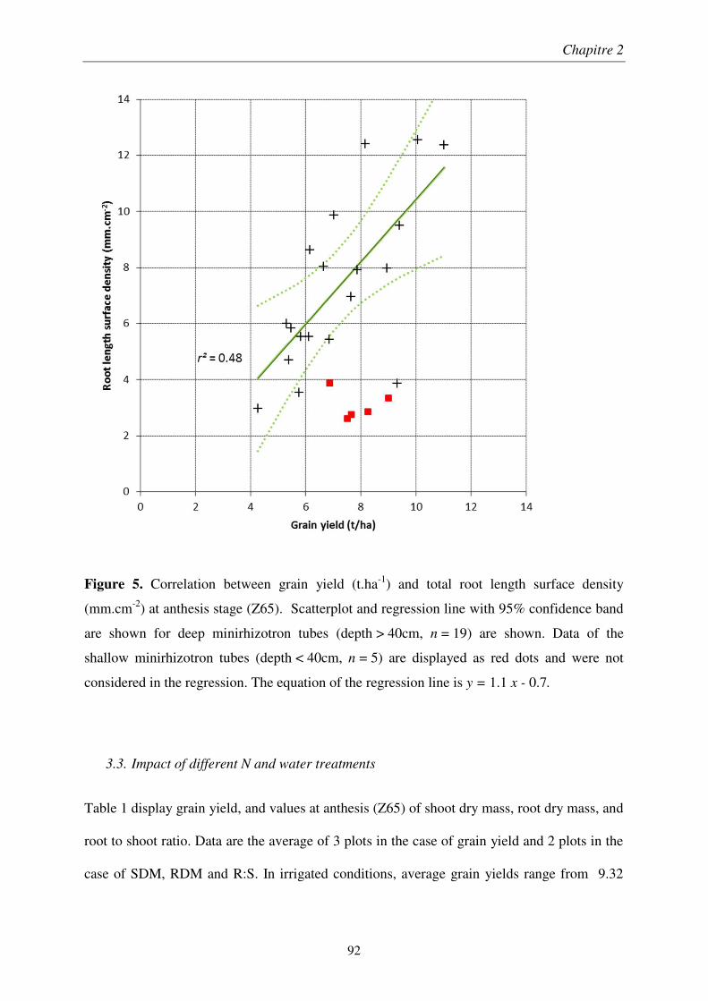
Chapitre 2

92

Figure 5. Correlation between grain yield (t.ha-1) and total root length surface density

(mm.cm-2) at anthesis stage (Z65). Scatterplot and regression line with 95% confidence band

are shown for deep minirhizotron tubes (depth > 40cm, n = 19) are shown. Data of the

shallow minirhizotron tubes (depth < 40cm, n = 5) are displayed as red dots and were not

considered in the regression. The equation of the regression line is y = 1.1 x - 0.7.

3.3. Impact of different N and water treatments

Table 1 display grain yield, and values at anthesis (Z65) of shoot dry mass, root dry mass, and

root to shoot ratio. Data are the average of 3 plots in the case of grain yield and 2 plots in the

case of SDM, RDM and R:S. In irrigated conditions, average grain yields range from 9.32

Chapitre 2

93

t.ha-1 to 8.16 t.ha-1 in I+N+ and I+N-, respectively, while in rainfed conditions, average grain

yields is lower and range from 5.62 t.ha-1 to 6.67 t.ha-1 in I-N+ and I-N-, respectively.

Table 2 shows the results of the analysis of variance (ANOVA) performed on grain yield

(GY15), and shoot dry mass (SDM), root dry mass (RDM) and root to shoot ratio (R:S)

measured at anthesis (Z65). The ANOVA was performed on these variables for the whole

experimental field (shallow soil conditions included), and the different irrigation treatments

(irrigated conditions and rainfed conditions). A significant effect on grain yield of the

irrigation treatment, the genotype and interactions between fertilization and irrigation (both p-

value < 0.001) is revealed. Fertilization has no significant effect on grain yield, unlike shoot

dry mass, root dry mass and R:S ratio (p-values < 0.01). ANOVA results from rainfed

conditions show a statistically significant effect of fertilization on grain yield and R:S ratio (p-

value < 0.001 and <0.01, respectively), while no significant effect has been found on shoot

dry mass and root dry mass. In addition, a significant interaction of genotype × fertilization on

root dry mass and R:S ratio (p-value < 0.001 and <0.01, respectively) is evidenced in rainfed

conditions.

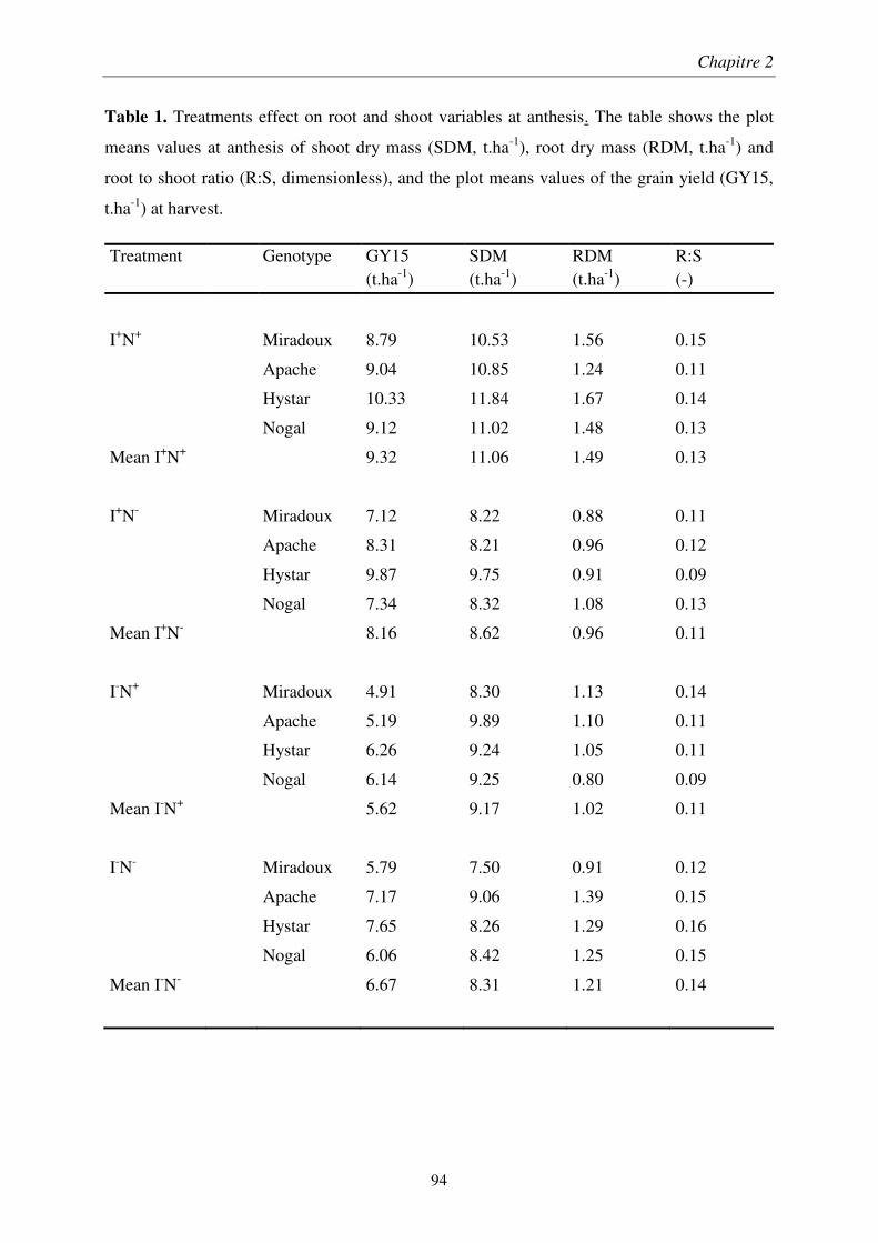
Chapitre 2

94

Table 1. Treatments effect on root and shoot variables at anthesis. The table shows the plot

means values at anthesis of shoot dry mass (SDM, t.ha-1), root dry mass (RDM, t.ha-1) and

root to shoot ratio (R:S, dimensionless), and the plot means values of the grain yield (GY15,

t.ha-1) at harvest.

Treatment

Genotype

GY15 (t.ha-1)

SDM (t.ha-1)

RDM (t.ha-1)

R:S (-)

I+N+ Miradoux 8.79 10.53 1.56 0.15

Apache 9.04 10.85 1.24 0.11

Hystar 10.33 11.84 1.67 0.14

Nogal 9.12 11.02 1.48 0.13

Mean I+N+ 9.32 11.06 1.49 0.13

I+N- Miradoux 7.12 8.22 0.88 0.11

Apache 8.31 8.21 0.96 0.12

Hystar 9.87 9.75 0.91 0.09

Nogal 7.34 8.32 1.08 0.13

Mean I+N- 8.16 8.62 0.96 0.11

I-N+ Miradoux 4.91 8.30 1.13 0.14

Apache 5.19 9.89 1.10 0.11

Hystar 6.26 9.24 1.05 0.11

Nogal 6.14 9.25 0.80 0.09

Mean I-N+ 5.62 9.17 1.02 0.11

I-N- Miradoux 5.79 7.50 0.91 0.12

Apache 7.17 9.06 1.39 0.15

Hystar 7.65 8.26 1.29 0.16

Nogal 6.06 8.42 1.25 0.15

Mean I-N- 6.67 8.31 1.21 0.14

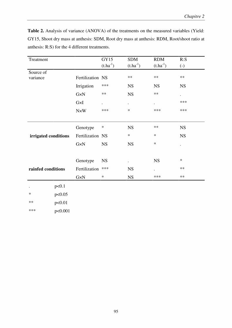
Chapitre 2

95

Table 2. Analysis of variance (ANOVA) of the treatments on the measured variables (Yield:

GY15, Shoot dry mass at anthesis: SDM, Root dry mass at anthesis: RDM, Root/shoot ratio at

anthesis: R:S) for the 4 different treatments.

Treatment

GY15 (t.ha-1)

SDM (t.ha-1)

RDM (t.ha-1)

R:S (-)

Source of variance Fertilization NS ** ** **

Irrigation *** NS NS NS

G×N ** NS ** .

G×I . . . ***

N×W *** * *** ***

Genotype * NS ** NS

irrigated conditions Fertilization NS * * NS

G×N NS NS * .

Genotype NS . NS *

rainfed conditions Fertilization *** NS . **

G×N * NS *** **

. p<0.1

* p<0.05

** p<0.01

*** p<0.001

Chapitre 2

96

Variation of Nitrogen nutrition index (NNI), mean root length surface density over

minirhizotron tubes (TRLSD) and the depth the bottom of the minirhizotron tubes between

the four (water, nitrogen) treatments is shown Table 3. NNI of N deprived treatments (I+N-

and I-N-) are not significantly different, but differ from other treatments resulting in 3

different groups (Fischer test, p < 5%). When excluding the zone of shallow soil of

minirhizotron installation, excluding the I+N- treatment, the other treatments do not differ in

terms maximum depth of minirhizotron tubes. Mean root length densities over the

minirhizotron depth were analysed at anthesis (Z65) only for those tubes of sufficient depths.

The average TRLSD measurements at anthesis range from 4.3 mm.cm-2 to 9.5 mm.cm-2,

similar to TRLSD measured in a previous experiment (Munoz-Romero et al., 2010).

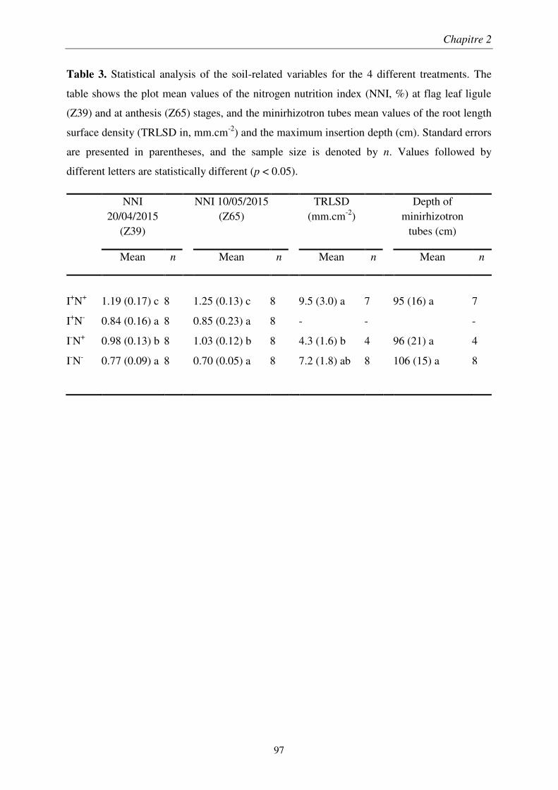
Chapitre 2

97

Table 3. Statistical analysis of the soil-related variables for the 4 different treatments. The

table shows the plot mean values of the nitrogen nutrition index (NNI, %) at flag leaf ligule

(Z39) and at anthesis (Z65) stages, and the minirhizotron tubes mean values of the root length

surface density (TRLSD in, mm.cm-2) and the maximum insertion depth (cm). Standard errors

are presented in parentheses, and the sample size is denoted by n. Values followed by

different letters are statistically different (p < 0.05).

  NNI 20/04/2015

(Z39)

NNI 10/05/2015 (Z65)

TRLSD (mm.cm-2)

Depth of minirhizotron

tubes (cm)

Mean n Mean n Mean n Mean n

I+N+ 1.19 (0.17) c 8 1.25 (0.13) c 8 9.5 (3.0) a 7 95 (16) a 7

I+N- 0.84 (0.16) a 8 0.85 (0.23) a 8 - - -

I-N+ 0.98 (0.13) b 8 1.03 (0.12) b 8 4.3 (1.6) b 4 96 (21) a 4

I-N- 0.77 (0.09) a 8 0.70 (0.05) a 8 7.2 (1.8) ab 8 106 (15) a 8

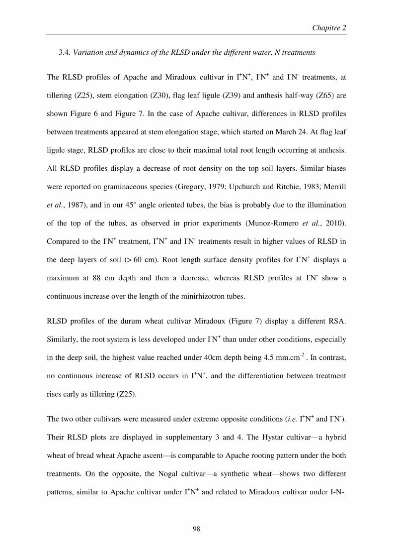
Chapitre 2

98

3.4. Variation and dynamics of the RLSD under the different water, N treatments

The RLSD profiles of Apache and Miradoux cultivar in I+N+, I-N+ and I-N- treatments, at

tillering (Z25), stem elongation (Z30), flag leaf ligule (Z39) and anthesis half-way (Z65) are

shown Figure 6 and Figure 7. In the case of Apache cultivar, differences in RLSD profiles

between treatments appeared at stem elongation stage, which started on March 24. At flag leaf

ligule stage, RLSD profiles are close to their maximal total root length occurring at anthesis.

All RLSD profiles display a decrease of root density on the top soil layers. Similar biases

were reported on graminaceous species (Gregory, 1979; Upchurch and Ritchie, 1983; Merrill

et al., 1987), and in our 45° angle oriented tubes, the bias is probably due to the illumination

of the top of the tubes, as observed in prior experiments (Munoz-Romero et al., 2010).

Compared to the I-N+ treatment, I+N+ and I-N- treatments result in higher values of RLSD in

the deep layers of soil (> 60 cm). Root length surface density profiles for I+N+ displays a

maximum at 88 cm depth and then a decrease, whereas RLSD profiles at I-N- show a

continuous increase over the length of the minirhizotron tubes.

RLSD profiles of the durum wheat cultivar Miradoux (Figure 7) display a different RSA.

Similarly, the root system is less developed under I-N+ than under other conditions, especially

in the deep soil, the highest value reached under 40cm depth being 4.5 mm.cm-2 . In contrast,

no continuous increase of RLSD occurs in I+N+, and the differentiation between treatment

rises early as tillering (Z25).

The two other cultivars were measured under extreme opposite conditions (i.e. I+N+ and I-N-).

Their RLSD plots are displayed in supplementary 3 and 4. The Hystar cultivar—a hybrid

wheat of bread wheat Apache ascent—is comparable to Apache rooting pattern under the both

treatments. On the opposite, the Nogal cultivar—a synthetic wheat—shows two different

patterns, similar to Apache cultivar under I+N+ and related to Miradoux cultivar under I-N-.

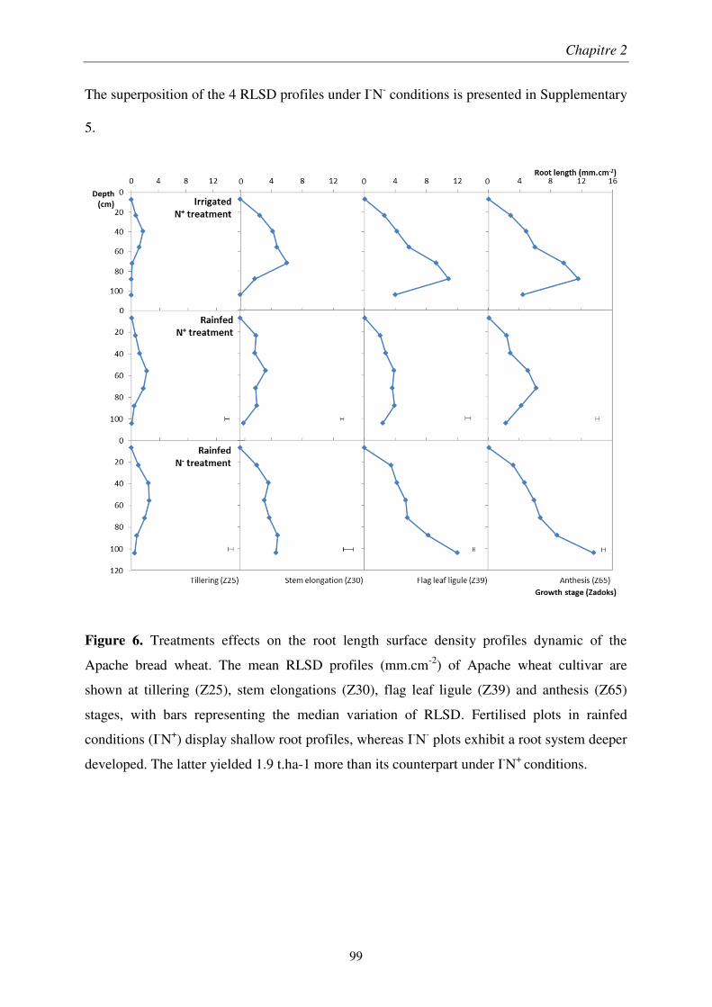
Chapitre 2

99

The superposition of the 4 RLSD profiles under I-N- conditions is presented in Supplementary

5.

Figure 6. Treatments effects on the root length surface density profiles dynamic of the

Apache bread wheat. The mean RLSD profiles (mm.cm-2) of Apache wheat cultivar are

shown at tillering (Z25), stem elongations (Z30), flag leaf ligule (Z39) and anthesis (Z65)

stages, with bars representing the median variation of RLSD. Fertilised plots in rainfed

conditions (I-N+) display shallow root profiles, whereas I-N- plots exhibit a root system deeper

developed. The latter yielded 1.9 t.ha-1 more than its counterpart under I-N+ conditions.

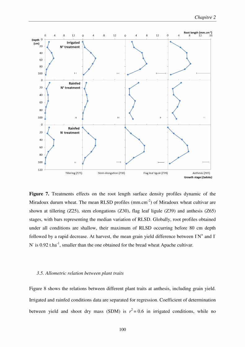
Chapitre 2

100

Figure 7. Treatments effects on the root length surface density profiles dynamic of the

Miradoux durum wheat. The mean RLSD profiles (mm.cm-2) of Miradoux wheat cultivar are

shown at tillering (Z25), stem elongations (Z30), flag leaf ligule (Z39) and anthesis (Z65)

stages, with bars representing the median variation of RLSD. Globally, root profiles obtained

under all conditions are shallow, their maximum of RLSD occurring before 80 cm depth

followed by a rapid decrease. At harvest, the mean grain yield difference between I-N+ and I-

N- is 0.92 t.ha-1, smaller than the one obtained for the bread wheat Apache cultivar.

3.5. Allometric relation between plant traits

Figure 8 shows the relations between different plant traits at anthesis, including grain yield.

Irrigated and rainfed conditions data are separated for regression. Coefficient of determination

between yield and shoot dry mass (SDM) is r2 = 0.6 in irrigated conditions, while no

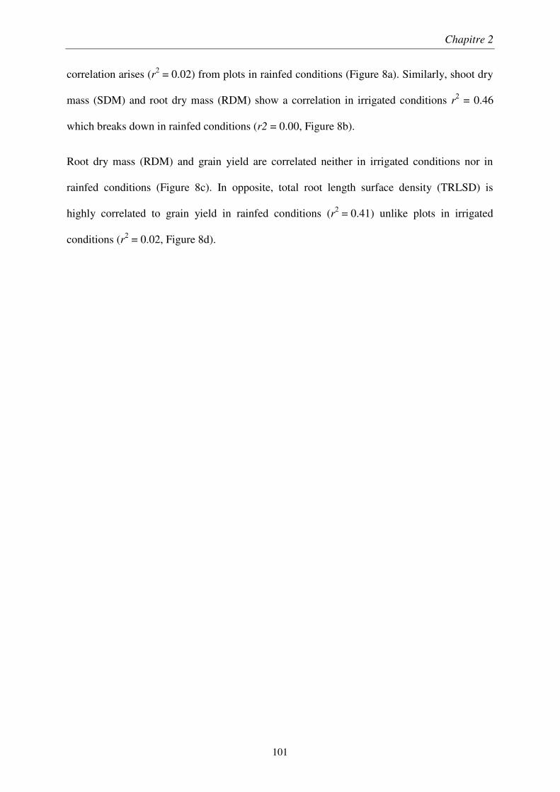
Chapitre 2

101

correlation arises (r2 = 0.02) from plots in rainfed conditions (Figure 8a). Similarly, shoot dry

mass (SDM) and root dry mass (RDM) show a correlation in irrigated conditions r2 = 0.46

which breaks down in rainfed conditions (r2 = 0.00, Figure 8b).

Root dry mass (RDM) and grain yield are correlated neither in irrigated conditions nor in

rainfed conditions (Figure 8c). In opposite, total root length surface density (TRLSD) is

highly correlated to grain yield in rainfed conditions (r2 = 0.41) unlike plots in irrigated

conditions (r2 = 0.02, Figure 8d).

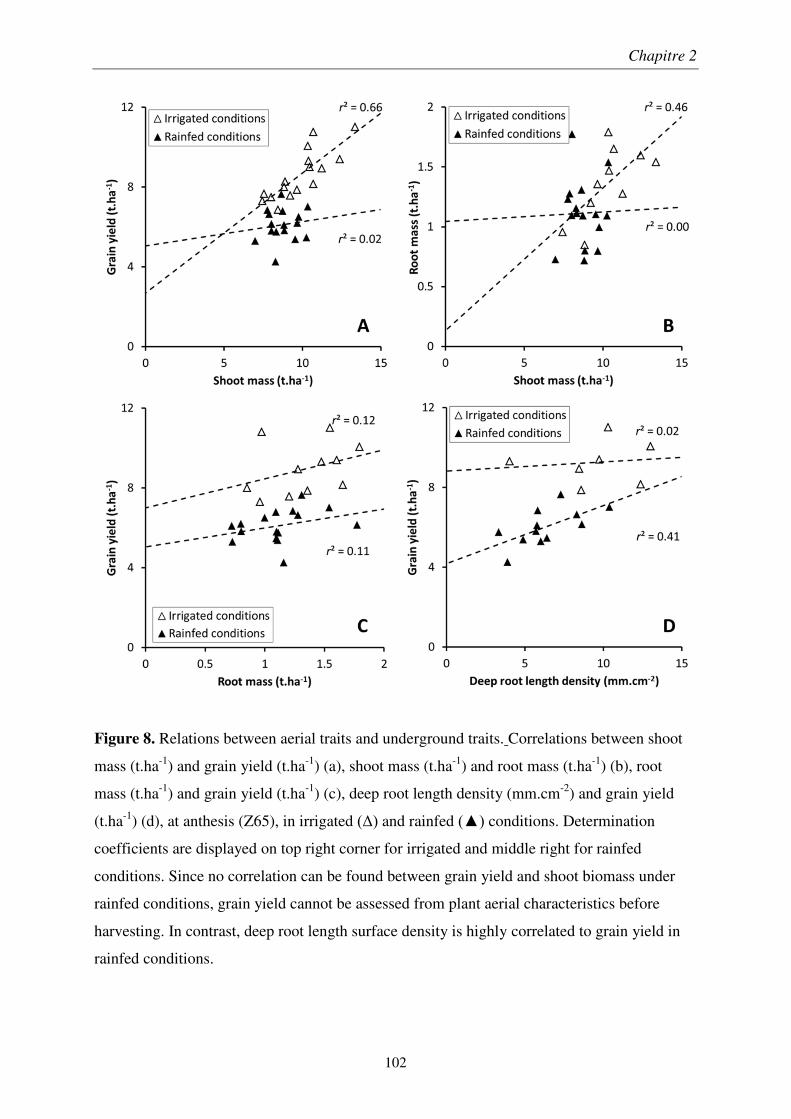
Chapitre 2

102

Figure 8. Relations between aerial traits and underground traits. Correlations between shoot

mass (t.ha-1) and grain yield (t.ha-1) (a), shoot mass (t.ha-1) and root mass (t.ha-1) (b), root

mass (t.ha-1) and grain yield (t.ha-1) (c), deep root length density (mm.cm-2) and grain yield

(t.ha-1) (d), at anthesis (Z65), in irrigated (Δ) and rainfed (▲) conditions. Determination

coefficients are displayed on top right corner for irrigated and middle right for rainfed

conditions. Since no correlation can be found between grain yield and shoot biomass under

rainfed conditions, grain yield cannot be assessed from plant aerial characteristics before

harvesting. In contrast, deep root length surface density is highly correlated to grain yield in

rainfed conditions.

Chapitre 2

103

4. Discussion

4.1. Minirhizotron methodology reliability

The conversion of the minirhizotrons data to actual root mass is a complex problem, and the

most straightforward solution is to consider an equivalent sampling volume. In our case, the

conversion factor value proposed in our study appears to be in agreement with the

depth-of-field previously estimated (Johnson et al., 2001; Zhang et al., 2008) at 2–3 mm. We

found a close depth-of-field value (ε = 0.35) using the mean SRL value for winter wheat crop

cultivars (Løes and Gahoonia, 2004). However, SRL may vary with N soil content and

genotype. Since it was not specifically measured, our estimation of DOP could be biased:

higher values of SRL would lead to smaller DOP, and vice versa.

The heavy-tailed skewedness distribution of the conversion factor (Supplementary 2) is a

result from the outliers in the RLSD measurements or from the auger sampling of root mass,

producing high values of ε×SRL. Thus, the median of the distribution is preferred to the mean

in order to have a statistic robust to outliers.

The model used for the root biomass profile in the shallow soil layers was affected by strong

assumptions. We assumed that the root biomass profile is fitted by a sigmoid, which was

approximated by 3 continuous affine functions. This estimated root biomass profile, coupled

to minirhizotron measurements led to R:S values in the range of previous observations

(Chaudhuri et al., 1990; Li et al., 2001; Allard et al., 2013) at anthesis in different growth

conditions. Moreover, the evolution with time of this R:S ratio is closely related to the R:S

ratio used in crop growth modelling (Keating et al., 2003) (Figure 4).

Our methodology differs from previous studies, by being less prone to the influence of

outlying values. A common way to estimate this type of conversion factor is the use of a

linear regression without y-intercept between minirhizotron data and gravimetric sampling

Chapitre 2

104

data. However, linear regressions are not robust to outliers, and coupled with the loss of

accuracy linked to the imposition of zero intercept, are not informative about the dispersion of

this conversion factor. A robust linear estimator, as the Theil-Sen estimator used in

agrophysics (Fernandes and G. Leblanc, 2005), could solve the issues related to outliers, but

not concerns about the y-intercept. The bootstrapping of the distribution of the individual

conversion values has intrinsically a zero intercept, and allows the computation of a non-

parametric confidence interval. Hence, this methodology does not rely on assumption on the

normality of the error, and hence is more suited for this type of calibration.

In spite of these advantages, this methodology could be challenged by the variations of the

SRL found variable among cultivars, among growth conditions (Løes and Gahoonia, 2004;

Nakhforoosh et al., 2014), i.e. not constant as we assumed. As a consequence, our R:S values

are only estimations. Nevertheless, the major contribution of the root mass is given by the top

layers root system, reducing the weight of the error on the estimation of root mass obtained by

RLSD conversion of minirhizotron data.

It appears that bias recorded in the shallow soil layers is a major issue linked to this

minirhizotron technique, and a special attention must be provided. Aluminium tapes could

have partially prevented illumination. A solution could consist in adding a large amount of

soil at the base of tube, and ensuring that plants centimeters around near tube base are

anchored. Globally, a deep soil— at least 90 cm— is required for the usage of this technique.

Presently, the major bottleneck of the technique resides in the absence of automatic image

processing. Even if accurate algorithm exists for washed roots imaged with flat scanners, they

appears not suited for minirhizotrons images, as the heterogeneity of the background—the

time-varying hue of the soil around the tube—prevents simple segmentation of roots.

Nevertheless, minirhizotrons allow repetitions of sampling without apparent field destruction,

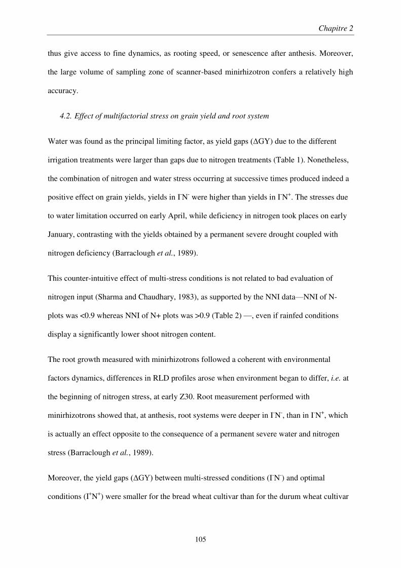
Chapitre 2

105

thus give access to fine dynamics, as rooting speed, or senescence after anthesis. Moreover,

the large volume of sampling zone of scanner-based minirhizotron confers a relatively high

accuracy.

4.2. Effect of multifactorial stress on grain yield and root system

Water was found as the principal limiting factor, as yield gaps (ΔGY) due to the different

irrigation treatments were larger than gaps due to nitrogen treatments (Table 1). Nonetheless,

the combination of nitrogen and water stress occurring at successive times produced indeed a

positive effect on grain yields, yields in I-N- were higher than yields in I-N+. The stresses due

to water limitation occurred on early April, while deficiency in nitrogen took places on early

January, contrasting with the yields obtained by a permanent severe drought coupled with

nitrogen deficiency (Barraclough et al., 1989).

This counter-intuitive effect of multi-stress conditions is not related to bad evaluation of

nitrogen input (Sharma and Chaudhary, 1983), as supported by the NNI data—NNI of N-

plots was <0.9 whereas NNI of N+ plots was >0.9 (Table 2) —, even if rainfed conditions

display a significantly lower shoot nitrogen content.

The root growth measured with minirhizotrons followed a coherent with environmental

factors dynamics, differences in RLD profiles arose when environment began to differ, i.e. at

the beginning of nitrogen stress, at early Z30. Root measurement performed with

minirhizotrons showed that, at anthesis, root systems were deeper in I-N-, than in I-N+, which

is actually an effect opposite to the consequence of a permanent severe water and nitrogen

stress (Barraclough et al., 1989).

Moreover, the yield gaps (ΔGY) between multi-stressed conditions (I-N-) and optimal

conditions (I+N+) were smaller for the bread wheat cultivar than for the durum wheat cultivar

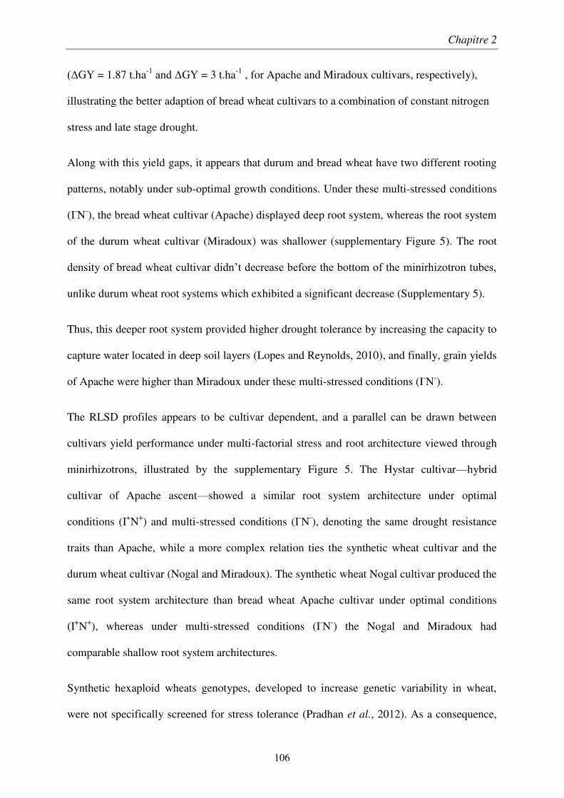
Chapitre 2

106

(ΔGY = 1.87 t.ha-1 and ΔGY = 3 t.ha-1 , for Apache and Miradoux cultivars, respectively),

illustrating the better adaption of bread wheat cultivars to a combination of constant nitrogen

stress and late stage drought.

Along with this yield gaps, it appears that durum and bread wheat have two different rooting

patterns, notably under sub-optimal growth conditions. Under these multi-stressed conditions

(I-N-), the bread wheat cultivar (Apache) displayed deep root system, whereas the root system

of the durum wheat cultivar (Miradoux) was shallower (supplementary Figure 5). The root

density of bread wheat cultivar didn’t decrease before the bottom of the minirhizotron tubes,

unlike durum wheat root systems which exhibited a significant decrease (Supplementary 5).

Thus, this deeper root system provided higher drought tolerance by increasing the capacity to

capture water located in deep soil layers (Lopes and Reynolds, 2010), and finally, grain yields

of Apache were higher than Miradoux under these multi-stressed conditions (I-N-).

The RLSD profiles appears to be cultivar dependent, and a parallel can be drawn between

cultivars yield performance under multi-factorial stress and root architecture viewed through

minirhizotrons, illustrated by the supplementary Figure 5. The Hystar cultivar—hybrid

cultivar of Apache ascent—showed a similar root system architecture under optimal

conditions (I+N+) and multi-stressed conditions (I-N-), denoting the same drought resistance

traits than Apache, while a more complex relation ties the synthetic wheat cultivar and the

durum wheat cultivar (Nogal and Miradoux). The synthetic wheat Nogal cultivar produced the

same root system architecture than bread wheat Apache cultivar under optimal conditions

(I+N+), whereas under multi-stressed conditions (I-N-) the Nogal and Miradoux had

comparable shallow root system architectures.

Synthetic hexaploid wheats genotypes, developed to increase genetic variability in wheat,

were not specifically screened for stress tolerance (Pradhan et al., 2012). As a consequence,

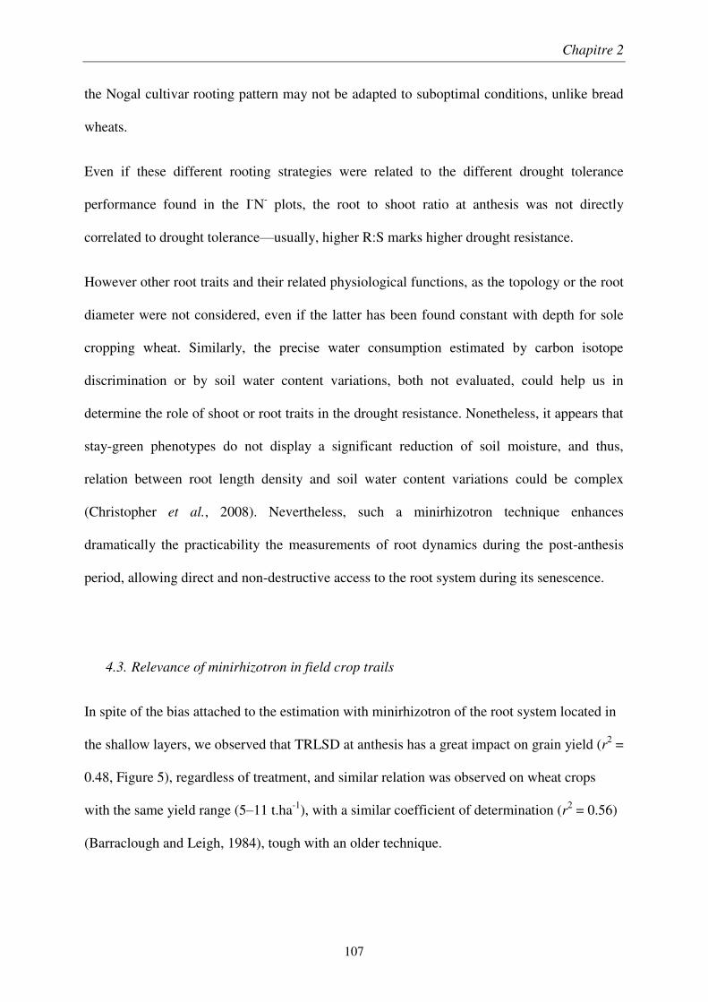
Chapitre 2

107

the Nogal cultivar rooting pattern may not be adapted to suboptimal conditions, unlike bread

wheats.

Even if these different rooting strategies were related to the different drought tolerance

performance found in the I-N- plots, the root to shoot ratio at anthesis was not directly

correlated to drought tolerance—usually, higher R:S marks higher drought resistance.

However other root traits and their related physiological functions, as the topology or the root

diameter were not considered, even if the latter has been found constant with depth for sole

cropping wheat. Similarly, the precise water consumption estimated by carbon isotope

discrimination or by soil water content variations, both not evaluated, could help us in

determine the role of shoot or root traits in the drought resistance. Nonetheless, it appears that

stay-green phenotypes do not display a significant reduction of soil moisture, and thus,

relation between root length density and soil water content variations could be complex

(Christopher et al., 2008). Nevertheless, such a minirhizotron technique enhances

dramatically the practicability the measurements of root dynamics during the post-anthesis

period, allowing direct and non-destructive access to the root system during its senescence.

4.3. Relevance of minirhizotron in field crop trails

In spite of the bias attached to the estimation with minirhizotron of the root system located in

the shallow layers, we observed that TRLSD at anthesis has a great impact on grain yield (r2 =

0.48, Figure 5), regardless of treatment, and similar relation was observed on wheat crops

with the same yield range (5–11 t.ha-1), with a similar coefficient of determination (r2 = 0.56)

(Barraclough and Leigh, 1984), tough with an older technique.

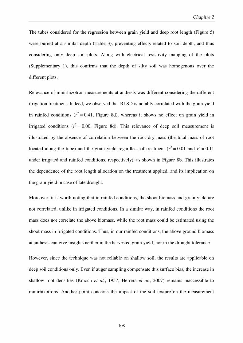
Chapitre 2

108

The tubes considered for the regression between grain yield and deep root length (Figure 5)

were buried at a similar depth (Table 3), preventing effects related to soil depth, and thus

considering only deep soil plots. Along with electrical resistivity mapping of the plots

(Supplementary 1), this confirms that the depth of silty soil was homogenous over the

different plots.

Relevance of minirhizotron measurements at anthesis was different considering the different

irrigation treatment. Indeed, we observed that RLSD is notably correlated with the grain yield

in rainfed conditions (r2 = 0.41, Figure 8d), whereas it shows no effect on grain yield in

irrigated conditions (r2 = 0.00, Figure 8d). This relevance of deep soil measurement is

illustrated by the absence of correlation between the root dry mass (the total mass of root

located along the tube) and the grain yield regardless of treatment (r2 = 0.01 and r2 = 0.11

under irrigated and rainfed conditions, respectively), as shown in Figure 8b. This illustrates

the dependence of the root length allocation on the treatment applied, and its implication on

the grain yield in case of late drought.

Moreover, it is worth noting that in rainfed conditions, the shoot biomass and grain yield are

not correlated, unlike in irrigated conditions. In a similar way, in rainfed conditions the root

mass does not correlate the above biomass, while the root mass could be estimated using the

shoot mass in irrigated conditions. Thus, in our rainfed conditions, the above ground biomass

at anthesis can give insights neither in the harvested grain yield, nor in the drought tolerance.

However, since the technique was not reliable on shallow soil, the results are applicable on

deep soil conditions only. Even if auger sampling compensate this surface bias, the increase in

shallow root densities (Kmoch et al., 1957; Herrera et al., 2007) remains inaccessible to

minirhizotrons. Another point concerns the impact of the soil texture on the measurement

Chapitre 2

109

bias, retraction of soil rich in clay would lead to larger gaps around tube, which would

stimulates the root growth, and thus, increases biases.

However, even if wheat plants traits at anthesis could give large insights of grain yield, post-

anthesis dynamic has high influence on the final grain yield (Passioura, 1977). Nevertheless,

this technique can evaluate rooting strategies, making it a valuable tool for cultivar

comparison, and for improving rooting models by in situ calibration.

5. Conclusion

In a Fluvisol limestone in a Mediterranean climate under irrigated and rainfed conditions,

wheat root length surface density estimated with minirhizotrons was fairly correlated with the

grain yield (r2 = 0.48). Moreover, under rainfed conditions, we observed that nitrogen stressed

plots exhibited higher grain yields, in correlation with larger root systems in deep soil

(r2 = 0.41), which was induced by a nitrogen deficiency before drought. In spite of biases in

root measurement in shallow soil, the minirhizotron technique provided rapid root length

density estimations, and with our non-parametric calibration methodology, its reliability has

been supported by the estimated root to shoot ratio at the different growth stages. However,

these biases prevent precise root length estimations, which require destructive measurements

and, moreover, the image processing remains a major bottleneck, and substantial

improvements in its automation would allow further exploitations of minirhizotron images.

The assessment of wheat SRL through the root diameters would indeed help to reduce the

amount of destructive sampling required, and thus, would greatly facilitate larger scale studies

of root traits. Further studies are necessary to evaluate the contribution of minirhizotron in

post-anthesis dynamics, which is substantially linked to crop grain yield. Nevertheless, this

Chapitre 2

110

technique would be a valuable tool in determining root traits of interest for drought resistance

and in enhancing accessibility to root measurement for crop breeding programs.

Acknowledgements

We thank Stéphane Jezequel and Xavier Le Bris for their helpful comments on early drafts of

this manuscript. We thank ARVALIS–Institut du végétal technical team located in Gréoux-

les-Bains. Special thanks are also expressed to Arnaud Chapelet and Hanah Kuttler for their

excellent assistance in the fieldwork.

Funding: This work was supported by grants from the FSOV [grant number FSOV-2012-E]

(French fund for plant breeding) and ARVALIS Institut du végétal.

Chapitre 2

111

Additional files

Additional file 1: Figure S1(.Tif). Electrical resistivity (Ω.m) map of the experimental field.

Green areas denote low electrical values, and red areas denote high electrical values. Positions

of minirhizotron tubes are displayed by white triangles (Δ). Low values of resistivity means

high soil depths, whereas high values of resistivity means low soil depths. Using soil coring

samples and minirhizotron depths, the scale relating depth to resistivity is estimated as

follows: 29–78 Ω.m = 71–120 cm, 78–126 Ω.m = 40–70 cm, 126–175 Ω.m = 30–40 cm, and

175–275 Ω.m < 30 cm.

Additional file 2: Figure S2(.Tif). Histogram of the conversion parameter (ε×SRL) to a

volumetric root biomass obtained with Eq. 2. The median value of the conversion parameter

is μ1/2 = 0.62 m2.g-1, leading to a depth of field of view of 3.5 mm by considering a specific

root length (SRL) value for winter wheat equals to 180 m.g-1

Additional file 3: Figure S3(.Tif). Effect of the different treatments on the dynamic of the

Hystar hybrid bread wheat root length surface density profiles (mm.cm-2) at different stages.

Mean root length surface density profiles of the Hystar wheat cultivar are shown at tillering

(Z25), stem elongations (Z30), flag leaf ligule (Z39) and anthesis (Z65) stages. Under the two

treatments monitored (optimal and water and nutrient coupled stress), both exhibit a deep

rooting profile pattern, optimal conditions peaking at 17.35 mm.cm-2 at anthesis(out of

figure). 

Additional file 4: Figure S4(.Tif). Effect of the different treatments on the dynamic of the

Nogal synthetic wheat root length surface density profiles (mm.cm-2) at different stages. Mean

root length surface density profiles of the Nogal synthetic wheat cultivar are shown at tillering

(Z25), stem elongations (Z30), flag leaf ligule (Z39) and anthesis (Z65) stages. Optimal and

stressful conditions shows contrasted rooting pattern. Under optimal conditions, this synthetic

Chapitre 2

112

wheat cultivar exhibits a deep root profile, as measured for the bread wheat Apache cultivar.

On the opposite, under stressful conditions, the root pattern developed is closer to the durum

wheat Miradoux cultivar measured. 

Additional file 5: Figure S5(.Tif). Comparison of the root length surface density profiles

obtained with minirhizotron technique at anthesis half-way (Z65) on average for each cultivar

under stressful conditions (I-N-). Similarities are found in the rooting profiles of Apache and

Hystar cultivars, and Miradoux and Nogal cultivars. A parallel may be drawn regarding their

grain yield, higher yields obtained by Apache and Hystar cultivars (7.17 t.ha-1, 7.65 t.ha-1,

respectively), lower yields obtained by Miradoux and Nogal cultivars (5.79 t.ha-1, 6.06 t.ha-1,

respectively).

References

Alexandratos N, Bruinsma J. 2012. World agriculture towards 2030/2050: the 2012 revision. ESA Working paper Rome, FAO.

Allard V, Martre P, Le Gouis J. 2013. Genetic variability in biomass allocation to roots in wheat is mainly related to crop tillering dynamics and nitrogen status. European Journal of Agronomy 46, 68–76.

Atkinson D. 1985. Spatial and temporal aspects of root distribution as indicated by the use of a root observation laboratory. Special publications series of the British Ecological Society.

Barraclough PB, Kuhlmann H, Weir AH. 1989. The Effects of Prolonged Drought and Nitrogen Fertilizer on Root and Shoot Growth and Water Uptake by Winter Wheat. Journal of Agronomy and Crop Science 163, 352–360.

Barraclough PB, Leigh RA. 1984. The growth and activity of winter wheat roots in the field: the effect of sowing date and soil type on root growth of high-yielding crops. The Journal of Agricultural Science 103, 59–74.

Barraclough PB, Weir AH, Kulhmann H. 1991. Factors Affecting the Growth and Distribution of Winter Wheat Roots Under Uk Field Conditions. In: McMichael BL,, In: Persson H, eds. Plant Roots and their Environment. Developments in Agricultural and Managed Forest Ecology. Elsevier, 410–417.

Brisson N, Gate P, Gouache D, Charmet G, Oury F-X, Huard F. 2010. Why are wheat yields stagnating in Europe? A comprehensive data analysis for France. Field Crops Research 119, 201–212.

Chapitre 2

113

Chaudhuri UN, Kirkham MB, Kanemasu ET. 1990. Root growth of winter wheat under elevated carbon dioxide and drought. Crop Science 30, 853–857.

Christopher JT, Manschadi AM, Hammer GL, Borrell AK. 2008. Developmental and physiological traits associated with high yield and stay-green phenotype in wheat. Australian Journal of Agricultural Research 59, 354.

Eberbach PL, Hoffmann J, Moroni SJ, Wade LJ, Weston LA. 2013. Rhizo-lysimetry: facilities for the simultaneous study of root behaviour and resource use by agricultural crop and pasture systems. Plant methods 9, 3.

Fernandes R, G. Leblanc S. 2005. Parametric (modified least squares) and non-parametric (Theil–Sen) linear regressions for predicting biophysical parameters in the presence of measurement errors. Remote Sensing of Environment 95, 303–316.

Gregory PJ. 1979. A periscope method for observing root growth and distribution in field soil. Journal of Experimental Botany 30, 205–214.

Herder GD, Van Isterdael G, Beeckman T, De Smet I. 2010. The roots of a new green revolution. Trends in Plant Science 15, 600–607.

Herrera JM, Stamp P, Liedgens M. 2007. Dynamics of root development of spring wheat genotypes varying in nitrogen use efficiency. Wheat Production in Stressed Environments. Springer, 197–201.

Iglesias A, Garrote L, Quiroga S, Moneo M. 2012. A regional comparison of the effects of climate change on agricultural crops in Europe. Climatic Change 112, 29–46.

Johnson MG, Tingey DT, Phillips DL, Storm MJ. 2001. Advancing fine root research with minirhizotrons. Environmental and Experimental Botany, 263–289.

Justes E, Mary B, Meynard J-M, Machet J-M, Thelier-Huche L. 1994. Determination of a Critical Nitrogen Dilution Curve for Winter Wheat Crops. Annals of Botany 74, 397–407.

Keating B., Carberry P., Hammer G., et al. 2003. An overview of APSIM, a model designed for farming systems simulation. European Journal of Agronomy 18, 267–288.

Kmoch HG, Ramig RE, Fox RL, Koehler FE. 1957. Root development of winter wheat as influenced by soil moisture and nitrogen fertilization. Agronomy journal 49, 20–26.

Langridge P. 2005. Molecular breeding of wheat and barley. In the Wake of Double Helix: From the Green Revolution to the Gene Revolution, 279–286. 

Li F-M, Liu X-L, Li S-Q. 2001. Effects of early soil water distribution on the dry matter partition between roots and shoots of winter wheat. Agricultural water management 49, 163–171.

Lobet G, Pages L, Draye X. 2011. A Novel Image-Analysis Toolbox Enabling Quantitative Analysis of Root System Architecture. Plant Physiology 157, 29–39.

Løes A-K, Gahoonia TS. 2004. Genetic variation in specific root length in Scandinavian wheat and barley accessions. Euphytica 137, 243–249.

Chapitre 2

114

Lopes MS, Reynolds MP. 2010. Partitioning of assimilates to deeper roots is associated with cooler canopies and increased yield under drought in wheat. Functional Plant Biology 37, 147.

Maeght J-L, Rewald B, Pierret A. 2013. How to study deep roots—and why it matters. Frontiers in Plant Science 4.

Manschadi AM, Hammer GL, Christopher JT, deVoil P. 2008. Genotypic variation in seedling root architectural traits and implications for drought adaptation in wheat (Triticum aestivum L.). Plant and Soil 303, 115–129.

Mathieu L, Lobet G, Tocquin P, Périlleux C. 2015. ‘Rhizoponics’: a novel hydroponic rhizotron for root system analyses on mature Arabidopsis thaliana plants. Plant methods 11, 3.

McCown RL, Hammer GL, Hargreaves JNG, Holzworth D, Huth NI. 1995. APSIM: an agricultural production system simulation model for operational research. Mathematics and computers in simulation 39, 225–231.

Merrill SD, Doering EJ, Reichman GA. 1987. Application of a minirhizotron with flexible, pressurized walls to a study of corn root growth. Minirhizotron Observation Tubes: Methods and Applications for Measuring Rhizosphere Dynamics, 131–143.

Metzner R, Eggert A, van Dusschoten D, Pflugfelder D, Gerth S, Schurr U, Uhlmann N, Jahnke S. 2015. Direct comparison of MRI and X-ray CT technologies for 3D imaging of root systems in soil: potential and challenges for root trait quantification. Plant methods 11, 17.

Monti A, Zatta A. 2009. Root distribution and soil moisture retrieval in perennial and annual energy crops in Northern Italy. Agriculture, Ecosystems & Environment 132, 252–259.

Mooney SJ, Pridmore TP, Helliwell J, Bennett MJ. 2012. Developing X-ray computed tomography to non-invasively image 3-D root systems architecture in soil. Plant and soil 352, 1–22.

Munoz-Romero V, Benítez-Vega J, López-Bellido L, López-Bellido RJ. 2010. Monitoring wheat root development in a rainfed vertisol: Tillage effect. European journal of agronomy 33, 182–187.

Nakhforoosh A, Grausgruber H, Kaul H-P, Bodner G. 2014. Wheat root diversity and root functional characterization. Plant and soil 380, 211–229.

Passioura JB. 1977. Grain yield, harvest index, and water use of wheat. Journal of the Australian Institute of Agricultural Science 43, 117–120.

Polomski J, Kuhn N, Waisel Y, Eshel A, Kafkafi U. 2002. Root research methods. Plant roots: The hidden half, 295–321.

Pradhan GP, Prasad PVV, Fritz AK, Kirkham MB, Gill BS. 2012. Effects of drought and high temperature stress on synthetic hexaploid wheat. Functional Plant Biology 39, 190.

Rellán-Álvarez R, Lobet G, Lindner H, et al. 2015. Multidimensional mapping of root responses to soil environmental cues using a luminescence-based imaging system. bioRxiv, 16931.

Chapitre 2

115

Reynolds MP, Pfeiffer WH, Royo C. 2000. Applying physiological strategies to improve yield potential. Durum Wheat Improvement in the Mediterranean Region: New Challenges. Options Mediterranèennes 40, 95–103.

Rich SM, Watt M. 2013. Soil conditions and cereal root system architecture: review and considerations for linking Darwin and Weaver. Journal of Experimental Botany 64, 1193–1208.

Sharma BR, Chaudhary TN. 1983. Wheat root growth, grain yield and water uptake as influenced by soil water regime and depth of nitrogen placement in a loamy sand soil. Agricultural Water Management 6, 365–373.

Tilman D, Balzer C, Hill J, Befort BL. 2011. Global food demand and the sustainable intensification of agriculture. Proceedings of the National Academy of Sciences 108, 20260–20264.

Trachsel S, Kaeppler SM, Brown KM, Lynch JP. 2011. Shovelomics: high throughput phenotyping of maize (Zea mays L.) root architecture in the field. Plant and Soil 341, 75–87.

Upchurch DR, Ritchie JT. 1983. Root observations using a video recording system in mini-rhizotrons. Agronomy journal 75, 1009–1015.

Waines JG, Ehdaie B. 2007. Domestication and crop physiology: roots of green-revolution wheat. Annals of Botany 100, 991–998.

Wang M-B, Zhang Q. 2009. Issues in using the WinRHIZO system to determine physical characteristics of plant fine roots. Acta Ecologica Sinica 29, 136–138.

Watt M, Moosavi S, Cunningham SC, Kirkegaard JA, Rebetzke GJ, Richards RA. 2013. A rapid, controlled-environment seedling root screen for wheat correlates well with rooting depths at vegetative, but not reproductive, stages at two field sites. Annals of Botany 112, 447–455.

Zadoks JC, Chang TT, Konzak CF, et al. 1974. A decimal code for the growth stages of cereals. Weed res 14, 415–421.

Zhang Z-S, Li X-R, Wang T, Wang X-P, Xue Q-W, Liu L-C. 2008. Distribution and Seasonal Dynamics of Roots in a Revegetated Stand of Artemisia ordosica Kracsh. in the Tengger Desert (North China). Arid Land Research and Management 22, 195–211.

Zhang X, Zhang X, Liu X, Shao L, Sun H, Chen S. 2015. Incorporating root distribution factor to evaluate soil water status for winter wheat. Agricultural Water Management 153, 32–41.

Chapitre 2

116

117 

Chapitre 3 : Un modèle étendu de l’impédance

des plantes : détection in situ des racines

François Postic Philippe Hinsinger 

Ran Erel Claude Doussan 

    

    

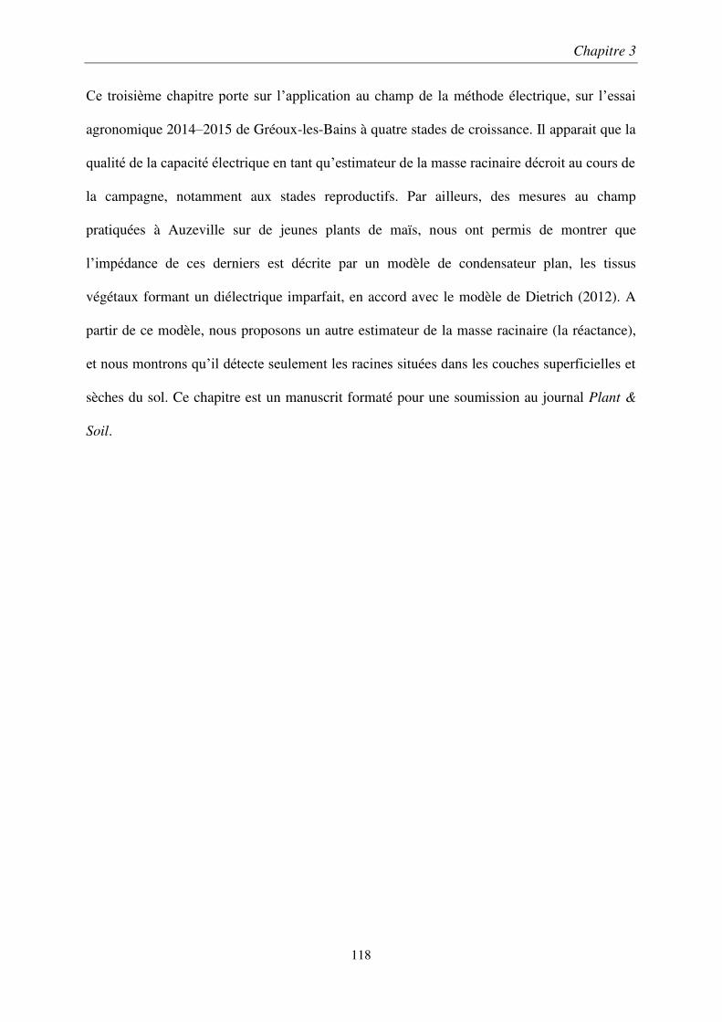
Chapitre 3

118

Ce troisième chapitre porte sur l’application au champ de la méthode électrique, sur l’essai

agronomique 2014–2015 de Gréoux-les-Bains à quatre stades de croissance. Il apparait que la

qualité de la capacité électrique en tant qu’estimateur de la masse racinaire décroit au cours de

la campagne, notamment aux stades reproductifs. Par ailleurs, des mesures au champ

pratiquées à Auzeville sur de jeunes plants de maïs, nous ont permis de montrer que

l’impédance de ces derniers est décrite par un modèle de condensateur plan, les tissus

végétaux formant un diélectrique imparfait, en accord avec le modèle de Dietrich (2012). A

partir de ce modèle, nous proposons un autre estimateur de la masse racinaire (la réactance),

et nous montrons qu’il détecte seulement les racines situées dans les couches superficielles et

sèches du sol. Ce chapitre est un manuscrit formaté pour une soumission au journal Plant &

Soil.

119

An extended model for plant impedance: in situ root sensing

François Postic1,2,*, Philippe Hinsinger3, Ran Erel3 and Claude Doussan2

1ARVALIS Institut du végétal, Paris, France.

2UMR EMMAH, INRA, UAPV, Domaine Saint-Paul, Site Agroparc, 84914 Avignon, France.

3 INRA, UMR Eco&Sols, Place Viala, 34060 Montpellier, France

*Corresponding author: francois.postic@paca.inra.fr

Tel.: +33432722266

Running title: Plant impedance for in situ root sensing

Submission date: 16 August 2016

Number of tables: 1

Number of figures: 6

Word count: 6495

Chapitre 3

120

Highlight

Plant tissues exhibit a dielectric loss like imperfect plate capacitors, and their reactance is an

in situ proxy of root mass located in dry soil down to 40 cm.

Abstract

Measurement of plant electrical capacitance is reported as a fast and cost-effective method for

estimating root system biomass. Recently, a new interpretation of the capacitance effect has

been given. This study extends this new model and shows that the electrical response of the

plant-soil system can be described by a plate capacitor separated by an imperfect dielectric

characterized by a complex dielectric value.

In the field, electrical impedance measurements have been performed on maize plants at

young stage (6-8 expanded leaves) and on wheat crop at four contrasted stages up to anthesis

in contrasted soil and hydric conditions. Shoot and root biomass were also measured

simultaneously.

Under well-watered conditions, in situ measurements on young maize satisfied the Dietrich

model, with an allometric relation between stem section and root mass. Nonetheless, in

accordance with our new model, in situ wheat root mass at late stage was linearly correlated

with the electrical reactance, though only in dry soil conditions, down to 40 cm below the soil

surface.

These results are consistent with our extension of the recent physical interpretation of plant

capacitance, and delineate in which case electrical measurements can be applied to root

sensing.

Chapitre 3

121

Key words

Root biomass, Triticum spp, Zea mays, electrical reactance, electrical capacitance, field

measurement.

Abbreviations

i – Unit Imaginary, number Dimensionless

m – Plant mass, grams, g

A – Area of overlap, square meters, m²

C – Parallel capacitance, Farads, F

G – Conductance, Siemens, S

L – Plate separation, meters, m

Rp – Parallel resistance Ohms, Ω

S – Root section, square meters, m²

X – Reactance, Ohms, Ω

Y – Admittance, Siemens, S

ε* – Complex permittivity of a material, F.m-1

ε’ – Real permittivity of a material, F.m-1

ε’’ – Imaginary permittivity of a material F.m-1

ω – Angular frequency, radians per seconds, rad.s-1

Chapitre 3

122

ω0 – Cut-off angular frequency, radians per seconds, rad.s-1

σ – Conductivity of a material, S.m-1

τ – Relaxation time, Seconds, s

Introduction

The global crop demand is estimated to double by 2050 (Tilman et al., 2011), while crop

yields could stagnate due to climate change (Asseng et al., 2014). Thus, the production of

cereals will not meet the needs of the world's population, especially when considering the

fertilizers crisis that could emerge—the prices of mineral phosphorus are increasingly volatile

(FAO of the United Nations, 2015) and expected to further increase (Brunelle et al., 2015),

while the production peak may occur within a few decades (Cordell et al., 2009) with the fast

depletion of the known reserves of rock phosphate (Peñuelas et al., 2013)—and the still

uncertain effects of the climate change on low-fertility soil (Lynch and St.Clair, 2004).

To face the future potential stagnation of yields, breeding programs shall aim at enhancing the

efficiency of crops under low soil fertility conditions (Lynch, 2007). Thus, the future breeding

programs should aim at higher efficiency in nutrient capture, a function ensured by the root

system of plants. Therefore, there is urgent need for identifying essential root traits in order to

design novel strategies of breeding for enhanced nutrients acquisition efficiency.

Unfortunately, all the current techniques to measure root traits in field-grown plants, although

allowing accurate and comprehensive characterisations, are destructive and time consuming.

In this context, a method that enhances the practicability of root measurement would be

highly relevant.

Chapitre 3

123

Even if breeding programs concerning roots would use greenhouse facilities (Wasson et al.,

2012), thus benefiting from the current automated phenotyping systems (Jeudy et al., 2016),

the relevance of in situ conditions should be better exploited, for testing interactions between

environmental factors and genetics, which is needed given the plasticity of root system

architecture (Rich and Watt, 2013).

Bio-impedance based techniques, which are assumed to estimate the root mass using the

electrical capacitance of the plant, would largely simplify root studies. Even if the root mass is

a straightforward trait, it reveals the root to shoot ratio, a stress indicator induced by limited

soil resources (Atkinson, 2000).

Plant capacitance measurement is fast and non-destructive, and has thus been proposed as a

valuable tool for sensing root mass (Chloupek, 1972). Experiments applied to different

species under greenhouse and laboratory conditions have been showing promising results

(Chloupek, 1977; Kendall et al., 1982; Dalton, 1995; van Beem et al., 1998; Aulen and

Shipley, 2012). The measurement is done with a LCR meter, by imposing an alternative

current through the plant-soil system using two electrodes: the first electrode connected to the

stem and the second positioned in the surrounding soil. Initially, an empirical linear

relationship had been found between the root mass and the parallel capacitance (Chloupek,

1972). The capacitive effect appears when there is a polarisation of electrical charges through

a dielectric medium (i.e. an insulator) that separates two conductive elements. In root tissues,

it was hypothesized that the epidermis is the imperfect insulator of a bio-capacitor, while root

internal medium and soil solution constitutes the two conductive elements (Dalton, 1995;

Ellis et al., 2013a), which has been conceptualised as an equivalent capacitance electrical

circuit (Dalton, 1995), known as the Dalton model, explaining the proportionality between

root mass and capacitance.

Chapitre 3

124

The quality of electrical root mass sensing depends on the growth media and its homogeneity.

For example, the root mass of hybrid poplars (Populus deltoids × P. nigra) is more accurately

estimated in hydroponics than in field conditions (Preston et al., 2004). Experimental

observations show that soil moisture induces large variations in the quality of the root mass

estimation (Kendall et al., 1982; Nakhforoosh et al., 2014). It was hypothesized that low soil

moisture reduces the contact surface between the roots and the soil solution. Alternatives to

Dalton’s model have been proposed, emphasizing the root surface or the active root area

(Ellis et al., 2013a).

Despite these limitations of the plant capacitance theory, developments have been

accomplished concerning the measurement methodology (Postic and Doussan, 2016). This

was generally accomplished by considering the spectral response (i.e. over a range of input

signal frequencies) to isolate output from specific plant compartments (Ozier-Lafontaine and

Bajazet, 2005). Additionally, more applied usages of capacitance have been prospected, as its

heritability after selection (Svačina et al., 2014; Heřmanská et al., 2015) or as in the detection

of root related quantitative trait loci (Chloupek et al., 2006).

Recently, a major competing hypothesis has been proposed. From opposite results obtained

by the excision of roots in hydroponics (Ozier-Lafontaine and Bajazet, 2005; Dietrich et al.,

2012), Dietrich et al. (2012) proposed a re-interpretation of the electrical capacitance signal

from the plant-growth media system. Its model describes a parallel plate capacitor (PPC), in

which the first plate is the plant electrode, and the second is the plant cross-sectional area at

the water table level, where plates are separated by a perfect dielectric medium. This PPC

model states that (i) the capacitance correlates linearly with the sum of root cross-sectional

areas at the water table level, (ii) the capacitance is inversely proportional to the root mass,

and (iii) the roots under the water table (i.e. under the water surface in hydroponics) could not

be sensed. Moreover, along with a physical explanation of the cause of this phenomenon, this

Chapitre 3

125

new theory gives insights on the soil moisture effect on the electrical response in such

experiments.

The disagreements between the two theories (Dalton, 1995; Dietrich et al., 2012) leaves many

questions unsolved, since the issues related to in situ conditions—variability of soil moisture

and plant phenology—have not been yet tested. Furthermore, field application of bio-

impedance techniques to monitor the dynamics of root growth in crops has not been explored

yet, since there are currently no reports on the in situ application of such electrical

measurements at contrasted plant growth stages. Moreover the parallel-plate capacitor (PPC)

model proposed by Dietrich et al. (2012) does not include the resistive part of the output

signal and its variations as related to the measurement setup (Dalton, 1995).

In this study, we propose to i) extend the PPC model to full complex impedance and apply it

to young well-watered maize (Zea mays L.) plants, ii) test the applicability of capacitance to a

field survey on bread and durum wheat (Triticum aestivum L. and Triticum turgidum durum

L.) crop, from tillering to anthesis, iii) determine the required conditions for efficient root

measurement in the frame of the new theory, and finally iv) deducing depth of electrical

measurement with regards to root depth.

Theory

Extension of the PPC model for root impedance

Several explanations of the root capacitance have been proposed (Dalton, 1995; Ozier-

Lafontaine and Bajazet, 2005; Ellis et al., 2013b). In their revised model, Dietrich et al.

(2012) describe a physically equivalent electrical model for the root capacitance. In

hydroponics, they demonstrated that the emerged part of the root system is equivalent to a

Chapitre 3

126

parallel-plate capacitor, i.e. two conductive plates oriented horizontally in the plane of the

water table surface, with the root system acting as the dielectric material. A first plate is

orthogonal to the stem at the location of the plant electrode, and a second at the surface of the

water table. It is worth to notice that the orientation of the capacitor is orthogonal to the root

axes, which is opposite to the former Dalton’s and Ellis’ models (Dalton, 1995; Ellis et al.,

2013a).

Since the initial design of the PPC model emphasized the capacitance—to discuss the

efficiency of the capacitance as a root mass estimator—, it did not consider the resistive

component of the plant tissues. In such a PPC model, the calculations consider a lossless

dielectric medium—like in an ideal capacitor —, thus the resistive component of the system

impedance cannot be represented. An extension to full complex impedance is introduced with

the imperfect parallel-plate capacitor model (IPPC), where a conductive loss component is

added and expressed in the complex permittivity ε* of the dielectric medium:

𝜀∗ = 𝜀′ + 𝜀′′ (1)

𝜀∗ = 𝜀′ − 𝑖𝜎

𝜔 (2)

where ε’ and ε’’ describe the real and imaginary parts of the permittivity (Eq. 1), respectively,

and the electrical leaking current, which depends on the angular frequency (ω), is formalised

by a conductivity term σ (Eq.2). The application of this complex dielectric constant ε* to a

parallel-plate capacitor with an area of plate overlap A with a separation L (Figure 1), is most

simply expressed by its admittance (inverse of impedance):

𝑌 = 𝑖𝜔𝜀∗ 𝐴

𝐿 (3)

𝑌 = 𝜎𝐴

𝐿+ 𝑖𝜔𝜀′ 𝐴

𝐿 (4)

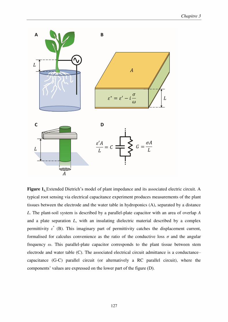
Chapitre 3

127

Figure 1. Extended Dietrich’s model of plant impedance and its associated electric circuit. A

typical root sensing via electrical capacitance experiment produces measurements of the plant

tissues between the electrode and the water table in hydroponics (A), separated by a distance

L. The plant-soil system is described by a parallel-plate capacitor with an area of overlap A

and a plate separation L, with an insulating dielectric material described by a complex

permittivity ε* (B). This imaginary part of permittivity catches the displacement current,

formalised for calculus convenience as the ratio of the conductive loss σ and the angular

frequency ω. This parallel-plate capacitor corresponds to the plant tissue between stem

electrode and water table (C). The associated electrical circuit admittance is a conductance–

capacitance (G-C) parallel circuit (or alternatively a RC parallel circuit), where the

components’ values are expressed on the lower part of the figure (D).

Chapitre 3

128

The admittance has a real and an imaginary components and represents an electrical circuit

with a conductor (G, in S—or expressed more classically as a resistance Rp, in Ω) and a

capacitor (C, in S) in parallel, identified by:

𝐺 = 𝜎𝐴

𝐿= 1/𝑅𝑝 (5) and 𝐶 = 𝜀′ 𝐴

𝐿 (6)

These relations (Eq. 5 and Eq.6) give us insights into the effects of the variation of the

system’s characteristic sizes on the electrical variables. Eq. 5 describes the effect of the

position of the stem electrode on the measured conductance and Eq. 6 on the capacitance.

The equations 5 and 6 state that an increase in the electrode distance to the base of the stem L

implies a decrease of both conductance G and capacitance C with L. As the resistance is the

inverse of the conductance, the resistance Rp increases linearly with L. Such behaviours have

been measured in previous experiments (Dalton, 1995) on bean (Phaseolus vulgare L.) plants

grown in hydroponics for both resistance and capacitance, by varying the stem electrode

position. Furthermore, a generalisation of this result on capacitance has been obtained

(Dietrich et al., 2012) on barley (Hordeum vulgare L.) plants by raising the plant tissues out

of hydroponic solutions, and thus increasing their plate separation L, i.e. the distance between

the stem electrode and the water table.

In the same manner, the effect of the variation of the area of overlap A is also given by these

equations, which describe a positive linear relation between area of plates overlap and both

conductance (Eq.5) or capacitance (Eq.6)

A more general property of the system is found by considering the relaxation time τ of the

equivalent circuit with the conductor (G) and a capacitor (C) in parallel:

𝜏 =1

𝐺× 𝐶 (7)

Chapitre 3

129

Replacing Eq.5 and Eq.6 into Eq.7 results to:

𝜏 =𝜀′

𝜎 (8)

By assuming that the permittivity is constant along the plant tissue and does not vary with the

section—more formally that the permittivity (both real and imaginary components) is not

function of L or A—, the partial derivatives of Eq. 12 with respect to either L or A give the

same relation:

𝜕𝜏

𝜕𝐿=

𝜕𝜏

𝜕𝐴= 0 (9)

Therefore, the relaxation time of the system would not vary with the system area (A) or the

electrode position (L).

Dietrich (2012) suggests that an allometric relation exists between the stem section (A)

intersecting the water table in hydroponics (or soil’s surface for a moist soil) and the root

mass (m). This allometric relationship can be expressed as a linear function f:

𝐴 = 𝑓(𝑚) = 𝛼1 + 𝛼2 × 𝑚 (10)

with α1 and α2 positive, and ideally α1 negligible compared to α2. By replacing the above

equation in Eq.5, Eq.6 and Eq.9, we obtain:

𝐺 =𝜎

𝐿× (𝛼1 + 𝛼2 × 𝑚) (11)

𝐶 =𝜀′

𝐿× (𝛼1 + 𝛼2 × 𝑚) (12)

𝜕𝜏

𝜕𝑚= 0 (13)

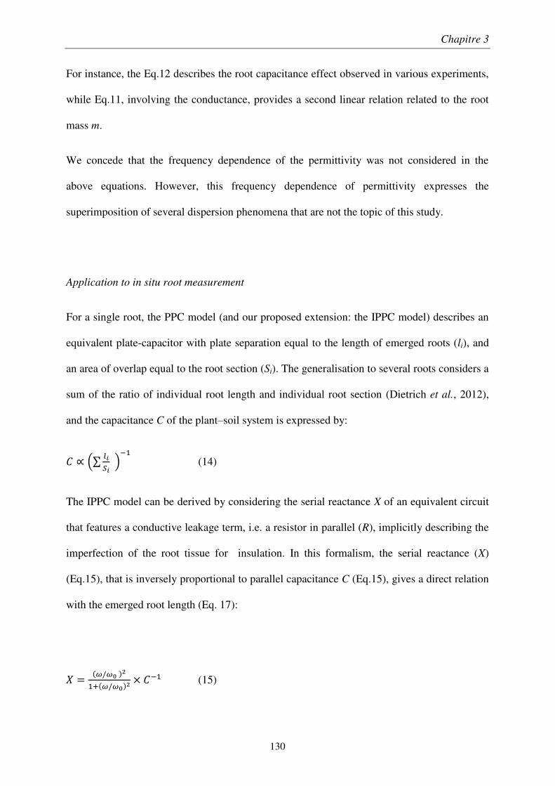
Chapitre 3

130

For instance, the Eq.12 describes the root capacitance effect observed in various experiments,

while Eq.11, involving the conductance, provides a second linear relation related to the root

mass m.

We concede that the frequency dependence of the permittivity was not considered in the

above equations. However, this frequency dependence of permittivity expresses the

superimposition of several dispersion phenomena that are not the topic of this study.

Application to in situ root measurement

For a single root, the PPC model (and our proposed extension: the IPPC model) describes an

equivalent plate-capacitor with plate separation equal to the length of emerged roots (li), and

an area of overlap equal to the root section (Si). The generalisation to several roots considers a

sum of the ratio of individual root length and individual root section (Dietrich et al., 2012),

and the capacitance C of the plant–soil system is expressed by:

𝐶 ∝ (∑𝑙𝑖𝑆𝑖

)−1

(14)

The IPPC model can be derived by considering the serial reactance X of an equivalent circuit

that features a conductive leakage term, i.e. a resistor in parallel (R), implicitly describing the

imperfection of the root tissue for insulation. In this formalism, the serial reactance (X)

(Eq.15), that is inversely proportional to parallel capacitance C (Eq.15), gives a direct relation

with the emerged root length (Eq. 17):

𝑋 =(𝜔/𝜔0 )2

1+(𝜔/𝜔0)2× 𝐶−1 (15)

Chapitre 3

131

𝜔0 =1

𝑅×𝐶 (16)

𝑋 ∝(𝜔/𝜔0 )2

1+(𝜔/𝜔0)2× ∑ 𝑙𝑖

𝑆𝑖 (17)

where ω is the angular frequency and ω0 is the cut-off frequency given by Eq. 16.

In the case of electrical measurements performed at a constant frequency, which is the

common protocol for such measurements, coupled with the assumption of a constant section

among roots, denoted S, the reactance X is directly proportional to the sum of the root lengths:

𝑋 ∝1

𝑆× ∑ 𝑙𝑖 (18)

By assuming also that root linear mass density—or its inverse, the so-called specific root

length (SRL)—does not vary along the root system, reactance is a proxy of the emerged root

mass mi:

𝑋 ∝1

𝑆×𝑆𝑅𝐿 × ∑ 𝑙𝑖 ∝ ∑𝑚𝑖 (19)

The generalisation to other substrates than hydroponics is done by considering the electrical

conductivity of the involved media. For pot grown plants, a dry soil acts as a poor conductor,

like air over water in hydroponics, while a wet soil act as a good conductor like the water in

hydroponics.

In crops, unlike in trees, root diameter classes have a narrow range of variation. Thus

reactance (X, in Ω) should be a proxy of the root mass between soil surface and the depth

where soil is wet.

Material and methods

Chapitre 3

132

In situ experiments on wheat

The experimental site is located in Gréoux-les-Bains (South of France). Four bread and durum

wheat cultivars (Miradoux, Apache, Hystar, Nogal) were sown in late October 2014 in

9.5 × 6.6 m2 plots at a sowing density of 300 seeds per m². Plots were divided to four

treatments, combining irrigation treatments (irrigated or rainfed, thereafter called I+ and I-,

respectively) and nitrogen fertilization levels (optimal or sub-optimal, thereafter called N+ and

N-, respectively). For the I+ treatments, a total of 189 mm water was applied in six intervals

from 15 April to 3 June 2015.

Electrical measurements—magnitude of impedance and phase angle—were performed on 28

January, 18 March, 4 April and 5 May 2015 corresponding to the 4 growth stages—tillering

(Z25), stem elongation (Z30), flag leaf ligule (Z39) and anthesis half-way (Z65)—with 3

plants per plot and 2 replicated plots. Acquisition was done with a SIP Fuchs III at 1 V input

voltage and 2 Hz frequency in a 3T configuration, merging input current (C1) and first

potential electrode (P1). Electrode C1–P1 was an alligator clamp (4 mm wide) positioned on

the plant (stem or leaf) 5 cm above the ground, the second potential electrode (P2) and the

output current electrode (C2), stainless rods (4 mm diameter) inserted 5 cm in the ground, at

a 20 cm and 30 cm radial distance, respectively, see illustration in Figure 1.

Surface root sampling was performed in the same plot just after electrical measurements.

Augers (40 mm diameter) were used to collect root sample in the same area as that of

electrical measurements, with two samples in the rows and a third between the rows. The

depth of sampling was 0–40 cm, and a sigmoid curve was used for root density estimation.

Central rows were sampled at 10–20 cm and 30–40 cm depth, and inter-rows were sampled at

30–40 cm. This sampling scheme was designed to integrate intra-row and inter-row variability

of the crop plots into the root measurement, while minimizing the number of sample. Roots

Chapitre 3

133

were washed from the soil for 10 min using a hydropneumatic elutriator, collected on 350 µm

sieves, oven dried at 70°C for 48h, and then weighted.

Deeper root mass (> 40 cm) were estimated using minirhizotrons tubes, that were imaged

with a CI-600 root scanner (CID Bio-Science, Camas, WA, USA) down to 110 cm below the

surface. The root length was measured and converted into root mass by using a specific root

length (SRL) equal to 180 m.g-1 (Løes and Gahoonia, 2004) and depth-of-field of 3 mm

(Zhang et al., 2008). Twenty-four plots were equipped: Hystar and Nogal cultivars were

equipped only in extreme conditions, i.e. I+N+ and I-N-.

Volumetric soil water content was measured weekly with a portable TDR (Time Domain

Reflectometry) PICO TRIME IPH64 over the period from 12 April 2015 to 10 May 2015—

i.e. between Z39 and Z65. Twenty-four tubes were installed in the same pattern as described

for the minirhizotron tubes, in the central row of plots, allowing the measurements every 10

cm. The median of the soil water content of the plots in the irrigated and rainfed situations

was computed for each layer.

In situ experiments on maize

The experimental site is located in the long term P-fertilizer trial of Auzeville (South-west of

France). Eight maize hybrids, having contrasting root traits, were sown in May 2015 with two

P fertilization levels at 6.7 grains per m². The whole plot was irrigated according to the

common agricultural practice.

Electrical measurements of parallel capacitance (C) and parallel resistance (Rp) were

performed using a portable LCR meter Agilent U1732A at 1V in a 2 terminals configuration,

at 1 kHz frequency. Electrode C1–P1 was an alligator clamp positioned 5 cm on the stem

Chapitre 3

134

above the ground, and electrode C2–P2, a stainless steel rod (4 mm diameter), was inserted at

10 cm with depth 10 cm. 222 plants were measured over the period of 9 to 12 June 2015,

corresponding to 6-8 leaf stage for different maize hybrids and P levels.

Plant and young root system were excavated with a shovel and roots separated from soil by

immersion in water and washing the root system. Roots and shoots were separated, weighted

for fresh weight and then dried at 60°C for dry weight determination.

Gravimetric soil water content of the 112 plots was measured the day of experiment, over the

0–15 cm depth horizon.

Statistical analyses

For the maize experiment, the coefficient of determination R2 (the square of the Pearson

product-moment correlation) was obtained by least-square linear regressions, between root

dry mass and electrical capacitance. For wheat experiments, an efficient robust linear

regression (the Theil-Sen estimator) applied to biophysical sensing in presence of

measurement errors (Fernandes and G. Leblanc, 2005) was used for the linear relation

between root dry mass and electrical capacitance. The Theil-Sen estimator (Theil, 1950; Sen,

1968), was computed, and residuals beyond the estimator maximum breakpoint were

discarded. This was achieved by computing the distribution of the residuals, used to

determine sample points belonging to the 1 −1

√2≈ 29.3% tails of their distribution, identified

as outliers. The determination coefficient R² (the square of the Pearson product-moment

correlation) was calculated with the remaining points.

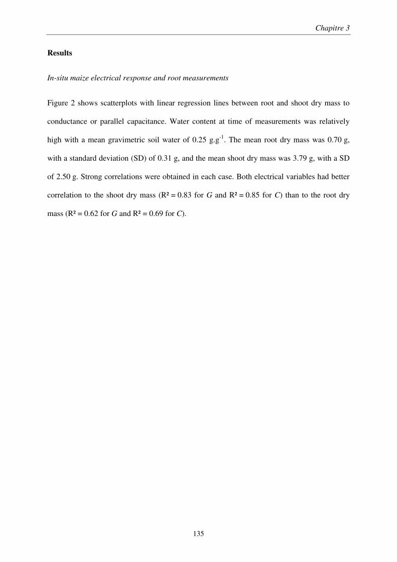
Chapitre 3

135

Results

In-situ maize electrical response and root measurements

Figure 2 shows scatterplots with linear regression lines between root and shoot dry mass to

conductance or parallel capacitance. Water content at time of measurements was relatively

high with a mean gravimetric soil water of 0.25 g.g-1. The mean root dry mass was 0.70 g,

with a standard deviation (SD) of 0.31 g, and the mean shoot dry mass was 3.79 g, with a SD

of 2.50 g. Strong correlations were obtained in each case. Both electrical variables had better

correlation to the shoot dry mass (R² = 0.83 for G and R² = 0.85 for C) than to the root dry

mass (R² = 0.62 for G and R² = 0.69 for C).

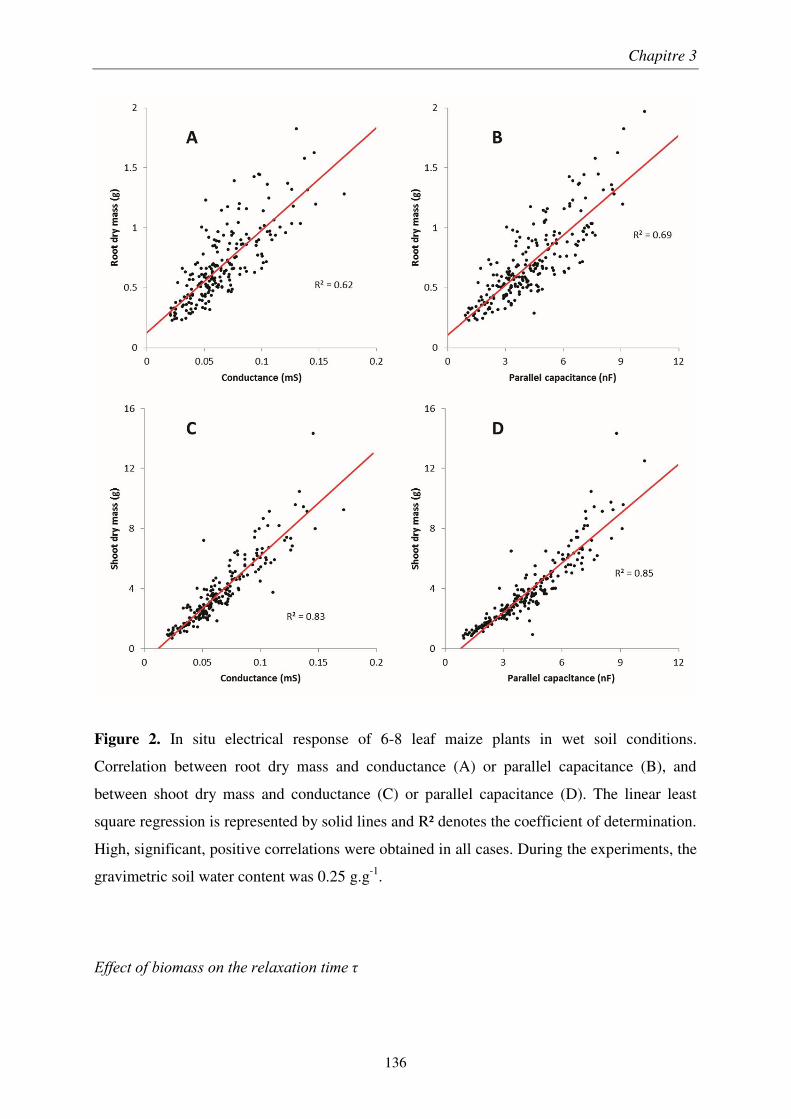
Chapitre 3

136

Figure 2. In situ electrical response of 6-8 leaf maize plants in wet soil conditions.

Correlation between root dry mass and conductance (A) or parallel capacitance (B), and

between shoot dry mass and conductance (C) or parallel capacitance (D). The linear least

square regression is represented by solid lines and R² denotes the coefficient of determination.

High, significant, positive correlations were obtained in all cases. During the experiments, the

gravimetric soil water content was 0.25 g.g-1.

Effect of biomass on the relaxation time τ

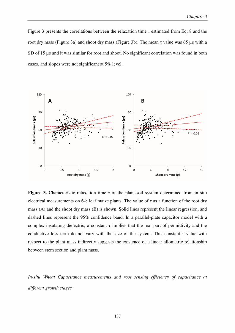
Chapitre 3

137

Figure 3 presents the correlations between the relaxation time τ estimated from Eq. 8 and the

root dry mass (Figure 3a) and shoot dry mass (Figure 3b). The mean τ value was 65 µs with a

SD of 15 µs and it was similar for root and shoot. No significant correlation was found in both

cases, and slopes were not significant at 5% level.

Figure 3. Characteristic relaxation time τ of the plant-soil system determined from in situ

electrical measurements on 6-8 leaf maize plants. The value of τ as a function of the root dry

mass (A) and the shoot dry mass (B) is shown. Solid lines represent the linear regression, and

dashed lines represent the 95% confidence band. In a parallel-plate capacitor model with a

complex insulating dielectric, a constant τ implies that the real part of permittivity and the

conductive loss term do not vary with the size of the system. This constant τ value with

respect to the plant mass indirectly suggests the existence of a linear allometric relationship

between stem section and plant mass.

In-situ Wheat Capacitance measurements and root sensing efficiency of capacitance at

different growth stages

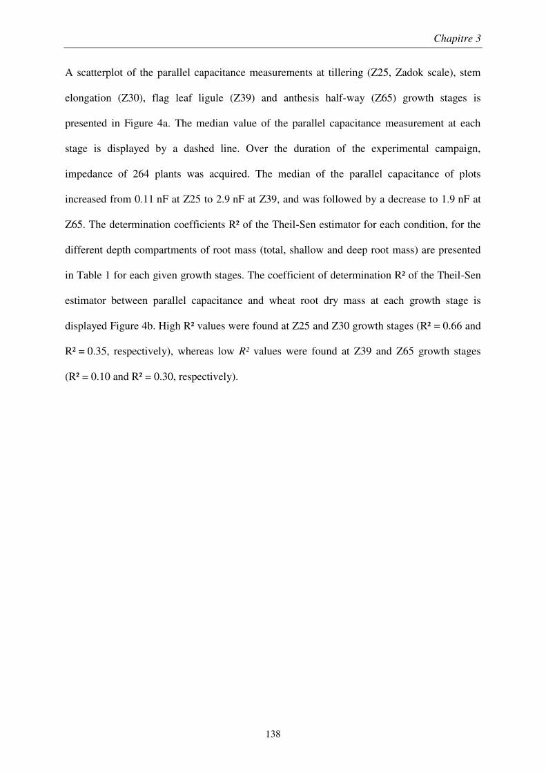
Chapitre 3

138

A scatterplot of the parallel capacitance measurements at tillering (Z25, Zadok scale), stem

elongation (Z30), flag leaf ligule (Z39) and anthesis half-way (Z65) growth stages is

presented in Figure 4a. The median value of the parallel capacitance measurement at each

stage is displayed by a dashed line. Over the duration of the experimental campaign,

impedance of 264 plants was acquired. The median of the parallel capacitance of plots

increased from 0.11 nF at Z25 to 2.9 nF at Z39, and was followed by a decrease to 1.9 nF at

Z65. The determination coefficients R² of the Theil-Sen estimator for each condition, for the

different depth compartments of root mass (total, shallow and deep root mass) are presented

in Table 1 for each given growth stages. The coefficient of determination R² of the Theil-Sen

estimator between parallel capacitance and wheat root dry mass at each growth stage is

displayed Figure 4b. High R² values were found at Z25 and Z30 growth stages (R² = 0.66 and

R² = 0.35, respectively), whereas low R² values were found at Z39 and Z65 growth stages

(R² = 0.10 and R² = 0.30, respectively).

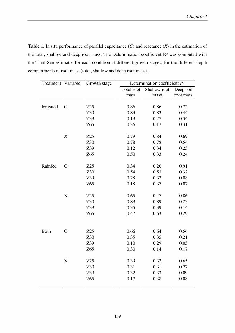
Chapitre 3

139

Table 1. In situ performance of parallel capacitance (C) and reactance (X) in the estimation of

the total, shallow and deep root mass. The Determination coefficient R² was computed with

the Theil-Sen estimator for each condition at different growth stages, for the different depth

compartments of root mass (total, shallow and deep root mass).

Treatment Variable Growth stage Determination coefficient R² Total root

mass Shallow root

mass Deep soil root mass

Irrigated C Z25 0.86 0.86 0.72 Z30 0.83 0.83 0.44 Z39 0.19 0.27 0.34 Z65 0.36 0.17 0.31 X Z25 0.79 0.84 0.69 Z30 0.78 0.78 0.54 Z39 0.12 0.34 0.25 Z65 0.50 0.33 0.24 Rainfed C Z25 0.34 0.20 0.91 Z30 0.54 0.53 0.32 Z39 0.28 0.32 0.08 Z65 0.18 0.37 0.07 X Z25 0.65 0.47 0.86 Z30 0.89 0.89 0.23 Z39 0.35 0.39 0.14 Z65 0.47 0.63 0.29 Both C Z25 0.66 0.64 0.56 Z30 0.35 0.35 0.21 Z39 0.10 0.29 0.05 Z65 0.30 0.14 0.17 X Z25 0.39 0.32 0.65 Z30 0.31 0.31 0.27 Z39 0.32 0.33 0.09 Z65 0.17 0.38 0.08

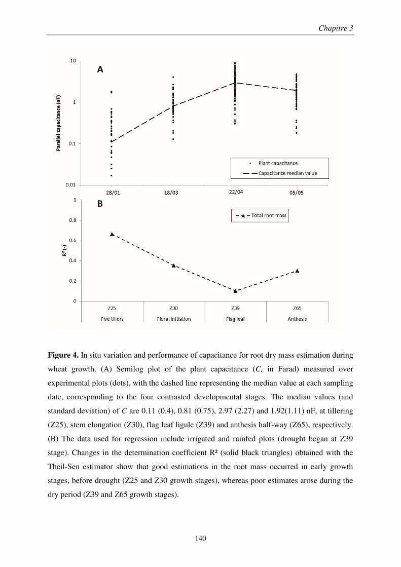
Chapitre 3

140

Figure 4. In situ variation and performance of capacitance for root dry mass estimation during

wheat growth. (A) Semilog plot of the plant capacitance (C, in Farad) measured over

experimental plots (dots), with the dashed line representing the median value at each sampling

date, corresponding to the four contrasted developmental stages. The median values (and

standard deviation) of C are 0.11 (0.4), 0.81 (0.75), 2.97 (2.27) and 1.92(1.11) nF, at tillering

(Z25), stem elongation (Z30), flag leaf ligule (Z39) and anthesis half-way (Z65), respectively.

(B) The data used for regression include irrigated and rainfed plots (drought began at Z39

stage). Changes in the determination coefficient R² (solid black triangles) obtained with the

Theil-Sen estimator show that good estimations in the root mass occurred in early growth

stages, before drought (Z25 and Z30 growth stages), whereas poor estimates arose during the

dry period (Z39 and Z65 growth stages).

Chapitre 3

141

Effect of soil moisture on efficiency of the electrical root estimators

A bar plot of the coefficient of determination R² of the Theil-Sen estimator between the root

dry mass and parallel capacitance C, and between the root dry mass and reactance (X), under

irrigated and rainfed conditions at Z39 and Z65 growth stages is shown in Figure 5. At flag

leaf ligule growth stage (Z39), the coefficients of determination R² show that under rainfed

conditions, reactance (X) was a better indicator for root mass than capacitance (C), while

under irrigated conditions both gave poorer predictors. At anthesis growth stage (Z65),

capacitance was a better predictor of the root dry mass in irrigated conditions than in rainfed

conditions, as shown by R² coefficients (R² = 0.36 and R² = 0.18, respectively), but reactance

was better performing than capacitance for both treatments with no effect of the irrigation

treatment on the coefficients of determination R² (R² = 0.50 and R² = 0.47, for irrigated and

rainfed conditions, respectively).

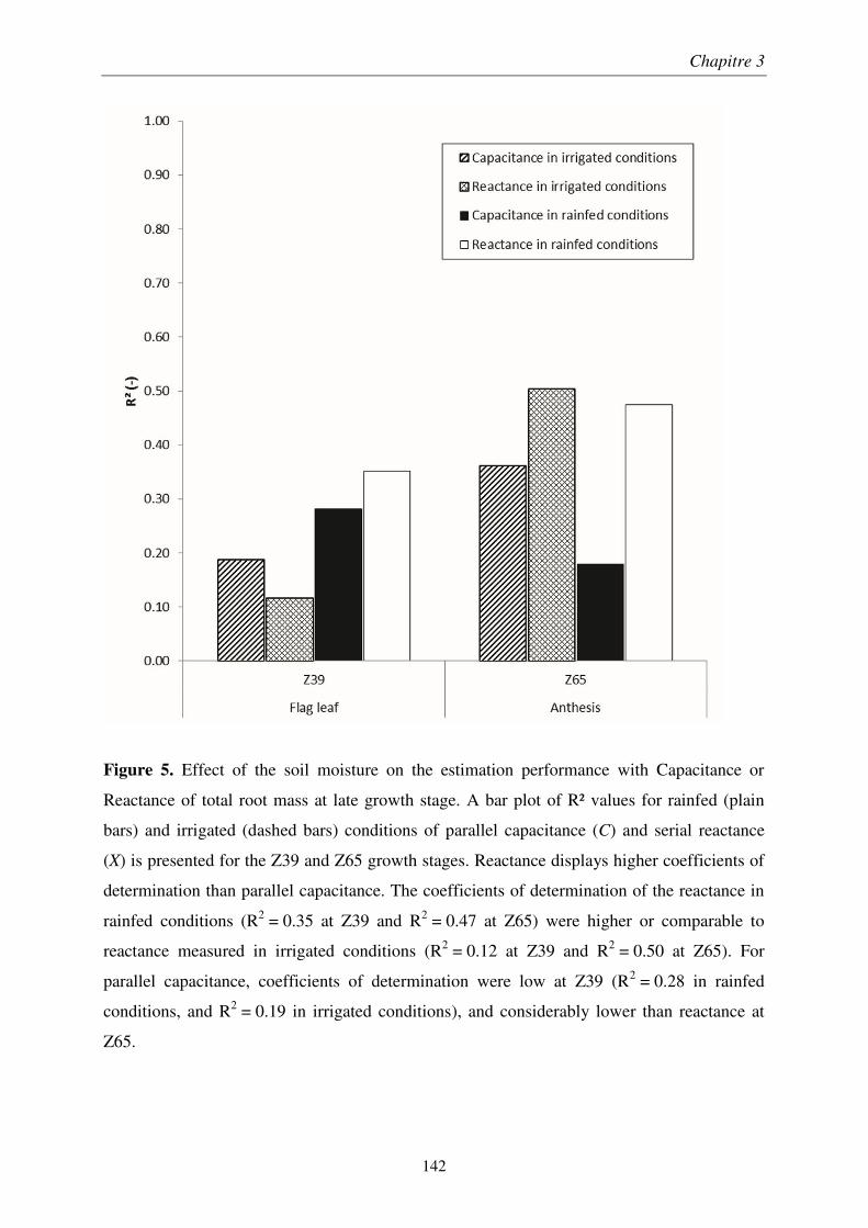
Chapitre 3

142

Figure 5. Effect of the soil moisture on the estimation performance with Capacitance or

Reactance of total root mass at late growth stage. A bar plot of R² values for rainfed (plain

bars) and irrigated (dashed bars) conditions of parallel capacitance (C) and serial reactance

(X) is presented for the Z39 and Z65 growth stages. Reactance displays higher coefficients of

determination than parallel capacitance. The coefficients of determination of the reactance in

rainfed conditions (R2 = 0.35 at Z39 and R2 = 0.47 at Z65) were higher or comparable to

reactance measured in irrigated conditions (R2 = 0.12 at Z39 and R2 = 0.50 at Z65). For

parallel capacitance, coefficients of determination were low at Z39 (R2 = 0.28 in rainfed

conditions, and R2 = 0.19 in irrigated conditions), and considerably lower than reactance at

Z65.

Chapitre 3

143

Reactance as a root mass proxy and depth of sensing in soil

Figures 6a and 6b show the R² obtained by the Theil-Sen estimator between reactance (X) and

the total root mass, the shallow root mass (0–40 cm), and the deep soil root mass (40–120 cm)

under irrigated and rainfed conditions at flag leaf ligule (Z39) and anthesis (Z65) growth

stages. The variations of volumetric soil water content during this period between 12 April

(Z39) and 10 May (Z65) 2015 are presented in Figures 6c and 6d, under irrigated and rainfed

conditions respectively, when the shallow soil horizons were drying. The coefficients of

determination R² obtained by reactance and capacitance at tillering (Z25) and stem elongation

(Z30) for each root compartment are also presented in Table 1.

For given root depth and irrigation treatment, the R² tended to increase between stages Z39

and Z65. In rainfed conditions, shallow root mass was better estimated (R² = 0.63) than total

root mass (R² = 0.47) or deep soil root mass (R² = 0.29). Under irrigated conditions, a similar

pattern occurred at Z39, while at anthesis stage an opposite trend was observed, the total root

mass displaying the highest R² values (R² = 0.50).

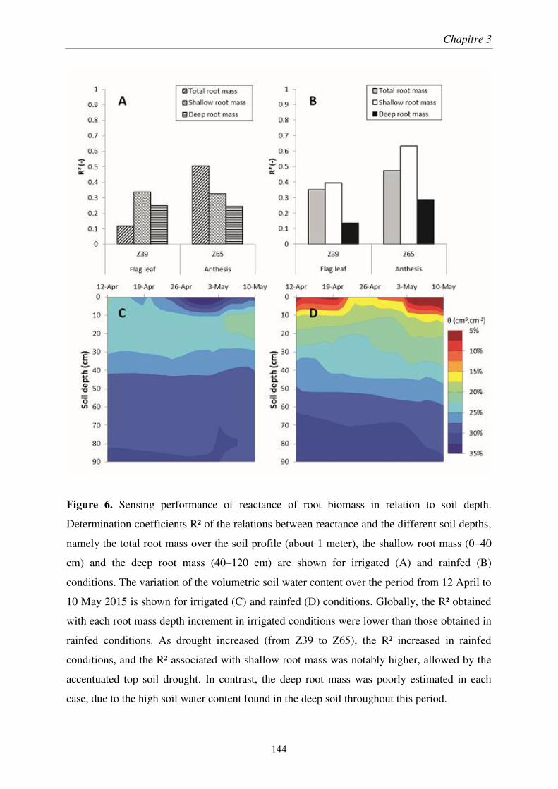
Chapitre 3

144

Figure 6. Sensing performance of reactance of root biomass in relation to soil depth.

Determination coefficients R² of the relations between reactance and the different soil depths,

namely the total root mass over the soil profile (about 1 meter), the shallow root mass (0–40

cm) and the deep root mass (40–120 cm) are shown for irrigated (A) and rainfed (B)

conditions. The variation of the volumetric soil water content over the period from 12 April to

10 May 2015 is shown for irrigated (C) and rainfed (D) conditions. Globally, the R² obtained

with each root mass depth increment in irrigated conditions were lower than those obtained in

rainfed conditions. As drought increased (from Z39 to Z65), the R² increased in rainfed

conditions, and the R² associated with shallow root mass was notably higher, allowed by the

accentuated top soil drought. In contrast, the deep root mass was poorly estimated in each

case, due to the high soil water content found in the deep soil throughout this period.

Chapitre 3

145

Discussion

Interactions of soil moisture and growth stage with capacitance

Electrical capacitance seemed to present a clear link to root mass only under precise

conditions. It appears that high soil water content coupled with early plant development stage

were the best conditions to obtain significant relations. In our experiments, the fair

performance of capacitance (C) for the root mass estimation on young maize plants (Figure

2a) and on young wheat plants (Figure 4b) supported Dalton’s model during early growth

stages and wet conditions. However, in the case of maize plants, the conductance (G)

correlated with the root mass as well (Figure 2b), and, moreover, we found that C or G were

better estimators of the shoot biomass (Figure 2a and 2c). This supports the hypothesis that

the aerial part of plants has a significant contribution in the capacitance effect when the soil is

at field capacity. It challenges the previous hypothesis stating that roots would contribute a

large fraction of the output signal under wet soil conditions, since it maximises the fraction of

root in contact with soil water (Dalton, 1995).

In previous studies (van Beem et al., 1998; Cseresnyés et al., 2016), the capacitance

measurements have been mostly performed on well-watered plant or on plants watered just

before the measurements, ensuring a high soil water content of the top soil layers. It has been

recently shown that under these conditions, the capacitance is more determined by the cross-

sectional area of root or stem with soil at the soil surface than by root tissues under the wet

soil surface (PPC model, Dietrich et al., 2012). The relation of capacitance with root biomass

would arise then from the allometric relation between stem section and plant mass. Such

linear relation between stem diameter and biomass has been reported across annual plant

species (Weiner and Thomas, 1992). However, cross-sectional area of stem and roots with

Chapitre 3

146

soil interface is extremely difficult to measure in the field and was thus not estimated in the

present study.

Implications of the IPPC model under wet soil conditions

The characterisation of plant tissue dielectric properties by a complex permittivity seems

validated from our results.

Firstly, Figures 2a and 2b support both the existence of an imaginary component permittivity

term—as shown by the occurrence of a capacitive and a conductive effect of the sensed plant

tissues. The increasing linear relations found for both electrical parameters satisfy Eq.11 and

Eq.12, for both root mass and shoot mass. The conductance and the parallel capacitance were

indeed more correlated with the shoot mass (Figure 2c and Figure 2d) than with the root mass.

This relation satisfies Eq.10, and thus, it indicates an allometric linear relation between stem

section and both root and shoot mass. The latter being more related to the stem, it would

produce higher correlations.

However, the non-null y-intercept of the linear relations found (p <0.001 in each case) is not

explained by the admittance in Eq.4, and its origin could lie in the prominence of soil in the

response of the equivalent plant–soil system electrical circuit. This statement was the aim of a

previous study, which identified the soil characteristics’ response (Ozier-Lafontaine and

Bajazet, 2005), modelled by a single resistive component connected to several parallel RC

circuit in series. if soil is the source of non-null intercept, which is probable, growing plants in

substrates with contrasted electrical properties would show variations in the linear relation

between C (or G) and root mass (or shoot mass)

Chapitre 3

147

The second evidence of the complex permittivity of plant tissue is illustrated by Figures 3a

and 3b. The results corroborate the relation derived in Eq.13, which establishes the

independence of the relaxation time from plant mass, for root and shoot parts, respectively.

We can assume that the dielectric medium properties do not vary with the plant mass at a

given developmental stage, since plants inner structure would not greatly vary. The flow of

current within the plant is not well established presently. Current could be transmitted within

the inner part of the stem (xylem and phloem) or at the surface of the stem (epidermis), or

both. However, it is probable that the source of conductive loss could originate from the

xylem or phloem vessels, which are filled continuously with ion-rich solutions, while the

epidermis could act as a perfect dielectric medium.

Moreover, the time relaxation τ found in our experiments was comparable to previous

estimates (Ozier-Lafontaine and Bajazet, 2005), and was notably comparable to the

characteristic time relaxation τ of the electrical equivalent circuit relating root mass and C.

Unexplained variance in electrical estimation of root mass

In spite of ensuring a constant electrode placement (position on the stem, distance from the

base of the stem), and beyond the inherited error of in-situ estimation of the root density using

auger for woody species (Levillain et al., 2011), we found that outliers of electrical values can

have a high frequency of occurrence in such a type of electrical estimation. This is illustrated

by the dispersion of C measures at the 4 growth stages, which range over two orders of

magnitude (Figure 4), whereas such a broad dispersion is not expected in the roots. A robust

linear estimator, as the Theil-Sen estimator, was required to obtain significant correlations.

Nevertheless, the high number of sample allowed us to discard a number of observations up to

Chapitre 3

148

the breakpoint limit of the Theil-Sen estimator without leading to systematic, artificial

correlation.

Application of capacitance for in situ root development monitoring

Determination of capacitance only appears to be a poorly effective tool for monitoring in situ

root development in heterogeneous soil. In fact, the efficiency, estimated from correlation R²

of parallel capacitance with root mass, varied with time (Figure 4b), and decreased after Z30,

showing non-significant correlation (R² =0.10 at Z39, and R² =0.30 at Z65). In addition, the

trend of the parallel capacitance at growth stages between Z39 and Z65 (Figure 4a) did not fit

with the general root growth curve. Thus, a direct comparison between electrical

measurements performed at different plant developmental stages may not lead to reliable

estimates of root mass change. Interestingly, our conclusions about the performance of

capacitance for monitoring the root development differ from recent pot experiments

(Cseresnyés et al., 2016). An important difference with our experiments concerns the soil

water content during the measurements. Pots were watered at their base just before

capacitance measurements, whereas our in situ measurements were performed within a large

range of soil moisture levels.

These implications of the effect of the soil moisture and growth stages on electrical

measurements could challenge conclusions of previous in situ experiments on wheat

(Nakhforoosh et al., 2014; Svačina et al., 2014; Heřmanská et al., 2015), because wet soil

conditions were used on fully grown plants, i.e. in the measurement conditions leading to the

poorest capacitance-based estimates of root mass in our field experiments. However, beyond

the fact that capacitance is a proxy of the plant cross-sectional area at the water table, our

conclusion on the minimum soil moisture required to perform accurate root estimation must

Chapitre 3

149

be ascertained. The soil electrical conductivity is linearly related to soil water content

(Samouëlian et al., 2005), but also to clay content (Shevnin et al., 2007)—and related to its

structure. Variations in the clay content can induce large variations in the conductivity. Lower

clay content could greatly increase the maximum threshold of soil moisture, and give access

to root sensing for roots located in wetter (or deeper) soil layers. 

Application of IPPC model for root estimation through electrical method

In accordance with our IPPC model, the root mass was better sensed by reactance than

capacitance at anthesis (Figure 5). This estimation of the root mass was enhanced by the low

soil water content found in rainfed conditions (Figure 6d), leaving the shallow soil roots

within an electrically resistive soil. Furthermore, as the water deficit increased, the

performance of reactance as a proxy of the shallow root mass increased (Figure 6b). In

contrast, under irrigated conditions, this performance of reactance for the shallow root

biomass was lower, due to the higher electrical conductivity of soil.

These observations would imply that conductivity of root tissues is higher than conductivity

of the dry soil. Surprisingly, the total root mass at anthesis under irrigated conditions

displayed significant correlation with reactance (R² = 0.50). A sufficient difference between

the conductivities of the soil and the root tissues could explain such a correlation. Although,

in these irrigated conditions, the shallow root mass was indeed poorly estimated, even if the

driest soil layers were located in the 0–40 cm.

Using reactance as a root mass proxy relies on the assumption that the root diameter does not

vary significantly (eq. 23). In wheat crops, the mean root section does not greatly vary with

depth (Fan et al., 2016) and, its variance remains small (Munoz-Romero et al., 2010). Thus,

Chapitre 3

150

with this low variance of root diameter, reactance remains a reliable proxy of root mass

located in poorly conductive soil.

Depth of sensing in different soil conditions

The effect of soil moisture is shown through the comparison of irrigated and rainfed

conditions, and by considering the surface and deep compartments of the root system.

Accuracy of root estimation is poor in irrigated conditions, for shallow and deep roots. On the

contrary, under rainfed conditions, the soil moisture was low in the 0–40 cm (mean moisture

θ = 15.6 cm3.cm-3, Figure 6d), while significantly higher in the deeper soil layers. In these dry

top soil conditions, the reactance estimation of root mass was highest (R² = 0.63), while in

deep soil layer prediction was poorer (R² = 0.29). This efficiency in the shallow layers shows

that root sensing via reactance requires a low conductivity medium, like a dry soil.

Unfortunately, it appears that deep soil root mass would not be accessible to the electrical

methods in this setting, due to the high conductivity of the surrounding soil because of its

high water content.

It is worth to notice that estimation of the total root mass was fairly good. Indeed, the total

root mass is dominated by the upper part of the root system (Fan et al., 2016), and thus,

largely estimated by the reactance of shallow root mass in dry soils. Thus, for sensing roots

located deeper in deeper soil layers, forced dehydration might be a practical tool (via

manipulations of irrigation, climatic conditions or by using a rain shelter). Additionally, in

sandy soils exhibiting a low clay content, predictions of deep roots mass are expected to be

more accurate.

Chapitre 3

151

In situ and greenhouse limitations for electrical root sensing

The growth stage seems a dominant factor in the accuracy of C as root mass estimator. Our

experiments show that early—before Z39—wheat root mass was highly correlated to C. Soil

water content was the second main factor in the accuracy of estimation. Most of the studies

claim that C measurements must be performed with adjunction of water at the base of the

stem, ensuring higher C values. In our experiments, early stage measurements were performed

under wet soil conditions, whereas measurements at later stages were also performed under

dry soil conditions, notably in the top soil.

Therefore, the design of electrical measurement campaign must consider the growth stage and

the soil water content, as discussed below. In greenhouse conditions, when early growth

stages representative of in-situ conditions and allometric relationship between characteristic

dimensions of plants—are prominent, it appears that parallel capacitance should be used as a

root mass sensor, in wet soil conditions only. In situ, later growth stages are accessible and

allometric relationships involving root mass can differ depending on the applied treatment.

Thus, if dry soil conditions can be achieved in the upper soil horizons, reactance could

provide a valuable estimation of the shallow root mass.

However, in greenhouse conditions root studies could also rely on the use of large scale

rhizotrons (Jeudy et al., 2016), providing reliable and numerous rooting information. In situ

surveys often emphasize the acquisition of deep soil moisture and nutrients (Manschadi et al.,

2010)—by roots at depth where this electrical method seems blind—, even though reduction

of the shallow root mass could be aimed as a trait for drought resistance (Zhu et al., 2005).

The use of electrical capacitance as a root estimator, and the derived methods proposed for

crop breeding (Chloupek et al., 2006; Svačina et al., 2014; Heřmanská et al., 2015), could be

challenged by the IPPC model and our study showed that (i) the capacitance was related to the

Chapitre 3

152

plant cross-sectional area at the water table, (ii) the capacitance was poorly correlated with

root mass at later developmental stages and (iii) the requirements of the IPPC model, namely

a dry growth medium, were probably not attained since the soil was well watered before

measurements. These innovative breeding results could have screened plant stem diameters,

as found by Dietrich, and thus, indirectly of the root masses.

Nevertheless, this kind of electrical method, using the reactance as a proxy of root mass,

would be applicable under drought conditions. This would make a valuable tool for breeding

crops for drought resistance, applicable to rain-shelter studies for simulating drought or to

drought-affected regions of the world such as the Mediterranean areas and semi-arid tropics.

Moreover, these results suggest that alternative measurement setups should be considered to

increase the fraction of output electrical current that have actually flowed through the roots,

by for example, placing a point electrode (instead of a rod) deeper in the soil.

Conclusion

By considering also the resistive component, and emphasising the linear relation between

electrical reactance and the total length of roots (a proxy of biomass for crops) located in low-

conductivity soil layers (i.e. dry soil layers), we showed here that the new physical approach

of the model is applicable to in situ wheat plants at reproductive stages. Under given

circumstances, electrical reactance reached a determination coefficient on root mass equal to

R² = 0.63, contributed mostly by the shallow roots (0–40 cm). Furthermore, electrical

capacitance was poorly correlated with root mass at reproductive stages. In situ, the

conditions required for a correlation with capacitance were a high soil moisture content

coupled to measurement of plants at a relatively young stage of growth. Besides, it appears

that the electrical capacitance was more correlated to shoot than to root mass.

Chapitre 3

153

By measuring impedance of young field-grown maize plants, we show that under wet soil

conditions and at early developmental stage, the extended electrical model involving a

complex permittivity medium was able to explain previously published results and satisfied a

linear relation between plant material and the electrical conductance. Moreover, the relaxation

time did not vary significantly with the plant mass, as predicted by the model. This indirectly

supports the allometric origin of the relation between root mass and capacitance under these

specific conditions.

Pot experiments with electrically contrasted substrates are required for the understanding of

the variations in the linear relation involving capacitance effect. Moreover, greenhouse and in

situ experiments should be designed for identifying requirement of the extended model to

drought conditions’ measurements, by quantifying precise soil conductivity threshold, and

then the precise soil moisture threshold of this method for a given soil texture. 

Nevertheless, the encouraging results with reactance for estimating shallow root mass under

in situ drought conditions make the electrical reactance a valuable tool to be further studied

and tested in plant breeding programs for drought resistance.

Acknowledgments

FP was funded by grants from the FSOV (French fund for plant breeding number FSOV

2012) involving INRA and ARVALIS–Institut du Végétal. The maize experiment was

conducted with funding from the European Community Seventh Framework Programme FP7-

KBBE-2011-5 under the grant agreement no.289300 (EURoot project). The authors thank the

ARVALIS–Institut du Végétal technical team located in Gréoux-les-Bains as well as the

Chapitre 3

154

technical staff of the INRA UE Auzeville. Special thanks are also expressed to Arnaud

Chapelet, Hanah Kuttler and Guillaume Meloux for their excellent assistance in the fieldwork

and during the numerous root washing sessions at Gréoux-les-Bains, and to Didier Arnal and

Esther Guillot at Auzeville.

Chapitre 3

155

References

Asseng S, Ewert F, Martre P, et al. 2014. Rising temperatures reduce global wheat production. Nature Climate Change 5, 143–147.

Atkinson D. 2000. Root characteristics: why and what to measure. In: Smit AL,, In: Bengough AG, In: Engels C, In: van Noordwijk M,, In: Pellerin S,, In: van de Geijn SC, eds. Root methods: a handbook. Springer-Verlag Berlin Heidelberg, 1–32.

Aulen M, Shipley B. 2012. Non-destructive estimation of root mass using electrical capacitance on ten herbaceous species. Plant and Soil 355, 41–49.

van Beem J, Smith ME, Zobel RW. 1998. Estimating root mass in maize using a portable capacitance meter. Agronomy Journal 90, 566–570.

Brunelle T, Dumas P, Souty F, Dorin B, Nadaud F. 2015. Evaluating the impact of rising fertilizer prices on crop yields. Agricultural Economics 46, 653–666.

Chloupek O. 1972. The relationship between electric capacitance and some other parameters of plant roots. Biologia Plantarum 14, 227–230.

Chloupek O. 1977. Evaluation of size of a plants root-system using its electrical capacitance. Plant and Soil 48, 525–532.

Chloupek O, Forster BP, Thomas WT. 2006. The effect of semi-dwarf genes on root system size in field-grown barley. Theoretical and Applied Genetics 112, 779–786.

Cordell D, Drangert J-O, White S. 2009. The story of phosphorus: Global food security and food for thought. Global Environmental Change 19, 292–305.

Cseresnyés I, Rajkai K, Takács T. 2016. Indirect monitoring of root activity in soybean cultivars under contrasting moisture regimes by measuring electrical capacitance. Acta Physiologiae Plantarum 38.

Dalton FN. 1995. In-situ root extent measurements by electrical capacitance methods. Plant and Soil 173, 157–165.

Dietrich RC, Bengough AG, Jones HG, White PJ. 2012. A new physical interpretation of plant root capacitance. Journal of Experimental Botany 63, 6149–6159.

Ellis T, Murray W, Kavalieris L. 2013a. Electrical capacitance of bean (Vicia faba) root systems was related to tissue density-a test for the Dalton Model. Plant and Soil 366, 575–584.

Ellis TW, Murray W, Paul K, Kavalieris L, Brophy J, Williams C, Maass M. 2013b. Electrical capacitance as a rapid and non-invasive indicator of root length. Tree Physiology 33, 3–17.

Fan J, McConkey B, Wang H, Janzen H. 2016. Root distribution by depth for temperate agricultural crops. Field Crops Research 189, 68–74.

FAO of the United Nations. 2015. World fertilizer trends and outlook to 2018. Rome: Food & Agriculture Organization of United Nations.

Chapitre 3

156

Fernandes R, G. Leblanc S. 2005. Parametric (modified least squares) and non-parametric (Theil–Sen) linear regressions for predicting biophysical parameters in the presence of measurement errors. Remote Sensing of Environment 95, 303–316.

Heřmanská A, Středa T, Chloupek O. 2015. Improved wheat grain yield by a new method of root selection. Agronomy for Sustainable Development 35, 195–202.

Jeudy C, Adrian M, Baussard C, et al. 2016. RhizoTubes as a new tool for high throughput imaging of plant root development and architecture: test, comparison with pot grown plants and validation. Plant Methods 12.

Kendall WA, Pederson GA, Hill RR. 1982. Root size estimates of red clover and alfalfa based on electrical capacitance and root diameter measurements. Grass and Forage Science 37, 253–256.

Levillain J, Thongo M’Bou A, Deleporte P, Saint-Andre L, Jourdan C. 2011. Is the simple auger coring method reliable for below-ground standing biomass estimation in Eucalyptus forest plantations? Annals of Botany 108, 221–230.

Løes A-K, Gahoonia TS. 2004. Genetic variation in specific root length in Scandinavian wheat and barley accessions. Euphytica 137, 243–249.

Lynch JP. 2007. TURNER REVIEW No. 14. Roots of the Second Green Revolution. Australian Journal of Botany 55, 493.

Lynch JP, St.Clair SB. 2004. Mineral stress: the missing link in understanding how global climate change will affect plants in real world soils. Field Crops Research 90, 101–115.

Manschadi AM, Christopher JT, Hammer GL, Devoil P. 2010. Experimental and modelling studies of drought‐adaptive root architectural traits in wheat ( Triticum aestivum L.). Plant Biosystems - An International Journal Dealing with all Aspects of Plant Biology 144, 458–462.

Munoz-Romero V, Benítez-Vega J, López-Bellido L, López-Bellido RJ. 2010. Monitoring wheat root development in a rainfed vertisol: Tillage effect. European journal of agronomy 33, 182–187.

Nakhforoosh A, Grausgruber H, Kaul H-P, Bodner G. 2014. Wheat root diversity and root functional characterization. Plant and soil 380, 211–229.

Ozier-Lafontaine H, Bajazet T. 2005. Analysis of root growth by impedance spectroscopy (EIS). Plant and Soil 277, 299–313.

Peñuelas J, Poulter B, Sardans J, et al. 2013. Human-induced nitrogen–phosphorus imbalances alter natural and managed ecosystems across the globe. Nature Communications 4.

Postic F, Doussan C. 2016. Benchmarking electrical methods for rapid estimation of root biomass. Plant Methods 12.

Preston GM, McBride RA, Bryan J, Candido M. 2004. Estimating root mass in young hybrid poplar trees using the electrical capacitance method. Agroforestry Systems 60, 305–309.

Chapitre 3

157

Rich SM, Watt M. 2013. Soil conditions and cereal root system architecture: review and considerations for linking Darwin and Weaver. Journal of Experimental Botany 64, 1193–1208.

Samouëlian A, Cousin I, Tabbagh A, Bruand A, Richard G. 2005. Electrical resistivity survey in soil science: a review. Soil and Tillage Research 83, 173–193.

Sen PK. 1968. Estimates of the Regression Coefficient Based on Kendall’s Tau. Journal of the American Statistical Association 63, 1379–1389.

Shevnin V, Mousatov A, Ryjov A, Delgado-Rodriquez O. 2007. Estimation of clay content in soil based on resistivity modelling and laboratory measurements. Geophysical Prospecting 55, 265–275.

Svačina P, Středa T, Chloupek O. 2014. Uncommon selection by root system size increases barley yield. Agronomy for sustainable development 34, 545–551.

Theil H. 1950. A Rank Invariant Method of Linear and Polynomial Regression Analysis. Nederlandse Akademie Wetenschappen Series A. 53, 386–392.

Tilman D, Balzer C, Hill J, Befort BL. 2011. Global food demand and the sustainable intensification of agriculture. Proceedings of the National Academy of Sciences 108, 20260–20264.

Wasson AP, Richards RA, Chatrath R, Misra SC, Prasad SS, Rebetzke GJ, Kirkegaard JA, Christopher J, Watt M. 2012. Traits and selection strategies to improve root systems and water uptake in water-limited wheat crops. Journal of experimental botany 63, 3485–3498.

Weiner J, Thomas SC. 1992. Competition and allometry in three species of annual plants. Ecology, 648–656.

Zhang Z-S, Li X-R, Wang T, Wang X-P, Xue Q-W, Liu L-C. 2008. Distribution and Seasonal Dynamics of Roots in a Revegetated Stand of Artemisia ordosica Kracsh. in the Tengger Desert (North China). Arid Land Research and Management 22, 195–211.

Zhu J, Kaeppler SM, Lynch JP. 2005. Topsoil foraging and phosphorus acquisition efficiency in maize (Zea mays). Functional Plant Biology 32, 749–762.

Chapitre 3

158

Résultats complémentaires

L’échantillonnage de biomasse racinaire par prélèvements étant lui-même sujet à une certaine

variabilité, la puissance d’estimation de la biomasse racinaire à partir de la réactance pourrait

être en réalité plus grande. En utilisant la réactance en tant que proxy de la biomasse racinaire,

nous pouvons évaluer la pertinence de son utilisation en conditions pluviales ou irriguées, et

nous pouvons juger de la quantité de réplications à effectuer pour discriminer des effets liés

aux génotypes ou aux traitements de fertilisation.

La variabilité intra-groupe (plantes du même génotype cultivées dans les mêmes conditions)

de ces mesures de réactance peut être jugée à travers une analyse de variance (ANOVA), à un

stade donné, par exemple ici floraison. En supposant que la distribution des valeurs de

réactance dans une parcelle suive une distribution normale, on constate que les données

permettent de déterminer un effet de la variété sur la réactance uniquement en pluvial

(Tableau Supp.1). Ceci indique que la variance des mesures est suffisamment faible pour

distinguer au moins deux groupes parmi les variétés. Dans notre cas seul Apache obtient des

mesures statistiquement différentes des trois autres variétés. En extrapolant les résultats pour

un nombre plus grand d’échantillons, qui suivent la même distribution statistique que nos

mesures expérimentales, il est possible d’évaluer l’effet de l’augmentation du nombre de

mesures par parcelle sur la possibilité de distinguer des génotypes (Tableau Supp.1).

À floraison, la réactance est un estimateur de la biomasse, uniquement en conditions de sol

peu humide. En effet, en conditions irriguées, nous constatons une absence d’effets

significatifs du génotype ou de la fertilisation sur les mesures de réactance. Ceci est

caractéristique d’une variabilité élevée des mesures de réactance dans une même situation.

Nous pouvons en déduire que les mesures de réactance sont dominées par d’autres facteurs

(erreurs de mesures liées au mauvais contraste électrique) que le génotype et l’apport en

Chapitre 3

159

intrants. Dans ces conditions irriguées, il est alors impossible d’estimer des valeurs de

réactance spécifiques à des génotypes, empêchant toute forme de sélection avec un critère

basé sur la réactance.

L’analyse de variance des mesures de réactance en conditions pluviales donne les limites de la

précision actuelle de cette méthode. En effet, l’apport d’azote induit une augmentation de la

masse racinaire superficielle, et devrait avoir un effet significatif sur les mesures de réactance

— celle-ci étant un estimateur de la biomasse racinaire des couches superficielles du sol. En

conditions pluviales, nous constatons un effet significatif de l’azote sur nos mesures de

réactance, issues de 6 mesures par situation. Toutefois, en simulant les tirages aléatoires, il

devrait être impossible de constater un effet de l’apport azoté avec 6 échantillons. Il est

probable que nos 6 mesures représentent le cas où la dispersion des mesures est faible.

D’après nos tirages aléatoires en conditions pluviales, un effet significatif de l’azote serait

mesurable à partir de 16 échantillons. Afin de réduire la source inexpliquée de la variance des

mesures, il faut améliorer la corrélation entre réactance et masse racinaire. Celle-ci est

dominée par le contraste électrique sol–racine, qui dépend principalement de l’humidité du

sol. L’utilisation de la réactance doit donc tenir compte des variations locales d’humidités.

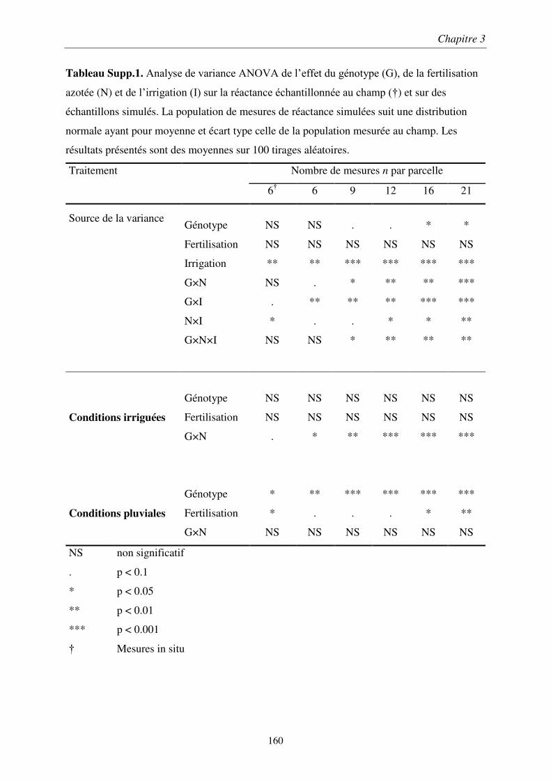
Chapitre 3

160

Tableau Supp.1. Analyse de variance ANOVA de l’effet du génotype (G), de la fertilisation

azotée (N) et de l’irrigation (I) sur la réactance échantillonnée au champ (†) et sur des

échantillons simulés. La population de mesures de réactance simulées suit une distribution

normale ayant pour moyenne et écart type celle de la population mesurée au champ. Les

résultats présentés sont des moyennes sur 100 tirages aléatoires.

Traitement Nombre de mesures n par parcelle

6† 6 9 12 16 21

Source de la variance Génotype NS NS . . * *

Fertilisation NS NS NS NS NS NS

Irrigation ** ** *** *** *** ***

G×N NS . * ** ** ***

G×I . ** ** ** *** ***

N×I * . . * * **

G×N×I NS NS * ** ** **

Génotype NS NS NS NS NS NS

Conditions irriguées Fertilisation NS NS NS NS NS NS

G×N . * ** *** *** ***

Génotype * ** *** *** *** ***

Conditions pluviales Fertilisation * . . . * **

G×N NS NS NS NS NS NS

NS non significatif

. p < 0.1

* p < 0.05

** p < 0.01

*** p < 0.001

† Mesures in situ

161

Conclusions

Conclusions

162

Cette thèse s’inscrit dans le cadre du développement méthodologique d’outils de phénotypage

racinaire, destinés à la sélection végétale du blé au champ. Les points déjà abordés dans la

discussion des chapitres précédents ne sont pas tous repris dans cette partie. L’accent est mis

ici sur l’apport des méthodes exposées à la caractérisation des traits racinaires, sur la fiabilité

de ces méthodes et sur les développements à réaliser pour une utilisation à plus grande

échelle. Enfin quelques résultats complémentaires, non-publiés, sont présentés afin de montrer

des perspectives d’application à la sélection végétale.

Bien que les minirhizotrons soient des outils invasifs, ils permettent un suivi direct des

dynamiques de croissance des systèmes racinaires. Ils nous ont ainsi permis de mettre en

évidence la réaction du système racinaire du blé en condition de faible apport en azote, à

l’aide de suivis de croissance dans des situations de cultures contrastées.

Les expériences menées sur le site expérimental de Gréoux-les-Bains durant la saison 2014-

2015 montrent un résultat étonnant concernant les rendements : les rendements en conditions

de stress hydrique seul sont inférieurs à ceux obtenus s’il y a à la fois stress hydrique et azoté.

À travers les données racinaires fournies par les minirhizotrons, il apparait que l’apparition

d’un stress de fertilisation azoté pendant la période végétative peut induire, suivant les

variétés, la mise en place d’un système racinaire colonisant plus la profondeur. La distribution

des racines, notamment celle des racines profondes, semble être liée à la capacité des plantes à

résister à la sécheresse (Lopes M.S. and Reynolds M.P., 2010). Ce type de phénomène a pu

être quantifié et mesuré grâce à l’aspect non destructif de cette méthode.

La fiabilité de l’estimation de la masse racinaire, au-delà de la couche 0-30 cm, à partir des

minirhizotrons à capteurs CCD de type scanner pourrait être conférée par la possibilité

d’échantillonner un grand volume de sol, sans qu’il soit nécessaire de corriger les aberrations

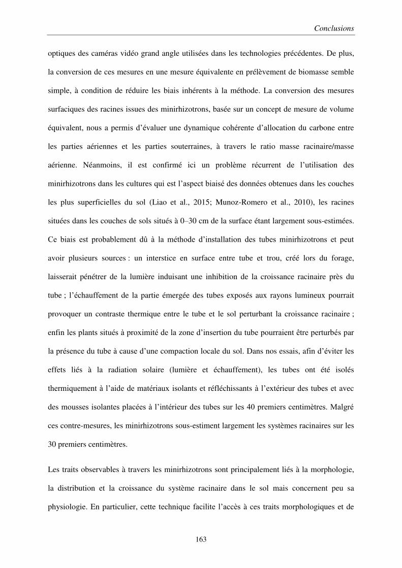
Conclusions

163

optiques des caméras vidéo grand angle utilisées dans les technologies précédentes. De plus,

la conversion de ces mesures en une mesure équivalente en prélèvement de biomasse semble

simple, à condition de réduire les biais inhérents à la méthode. La conversion des mesures

surfaciques des racines issues des minirhizotrons, basée sur un concept de mesure de volume

équivalent, nous a permis d’évaluer une dynamique cohérente d’allocation du carbone entre

les parties aériennes et les parties souterraines, à travers le ratio masse racinaire/masse

aérienne. Néanmoins, il est confirmé ici un problème récurrent de l’utilisation des

minirhizotrons dans les cultures qui est l’aspect biaisé des données obtenues dans les couches

les plus superficielles du sol (Liao et al., 2015; Munoz-Romero et al., 2010), les racines

situées dans les couches de sols situés à 0–30 cm de la surface étant largement sous-estimées.

Ce biais est probablement dû à la méthode d’installation des tubes minirhizotrons et peut

avoir plusieurs sources : un interstice en surface entre tube et trou, créé lors du forage,

laisserait pénétrer de la lumière induisant une inhibition de la croissance racinaire près du

tube ; l’échauffement de la partie émergée des tubes exposés aux rayons lumineux pourrait

provoquer un contraste thermique entre le tube et le sol perturbant la croissance racinaire ;

enfin les plants situés à proximité de la zone d’insertion du tube pourraient être perturbés par

la présence du tube à cause d’une compaction locale du sol. Dans nos essais, afin d’éviter les

effets liés à la radiation solaire (lumière et échauffement), les tubes ont été isolés

thermiquement à l’aide de matériaux isolants et réfléchissants à l’extérieur des tubes et avec

des mousses isolantes placées à l’intérieur des tubes sur les 40 premiers centimètres. Malgré

ces contre-mesures, les minirhizotrons sous-estiment largement les systèmes racinaires sur les

30 premiers centimètres.

Les traits observables à travers les minirhizotrons sont principalement liés à la morphologie,

la distribution et la croissance du système racinaire dans le sol mais concernent peu sa

physiologie. En particulier, cette technique facilite l’accès à ces traits morphologiques et de

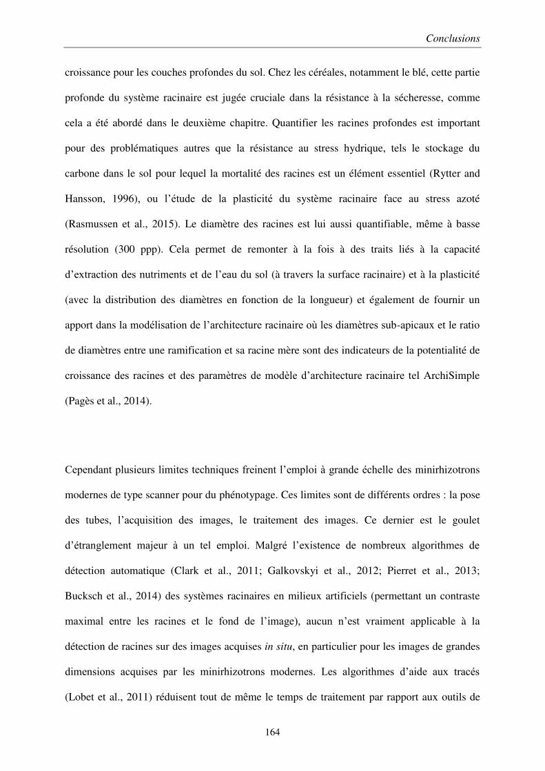
Conclusions

164

croissance pour les couches profondes du sol. Chez les céréales, notamment le blé, cette partie

profonde du système racinaire est jugée cruciale dans la résistance à la sécheresse, comme

cela a été abordé dans le deuxième chapitre. Quantifier les racines profondes est important

pour des problématiques autres que la résistance au stress hydrique, tels le stockage du

carbone dans le sol pour lequel la mortalité des racines est un élément essentiel (Rytter and

Hansson, 1996), ou l’étude de la plasticité du système racinaire face au stress azoté

(Rasmussen et al., 2015). Le diamètre des racines est lui aussi quantifiable, même à basse

résolution (300 ppp). Cela permet de remonter à la fois à des traits liés à la capacité

d’extraction des nutriments et de l’eau du sol (à travers la surface racinaire) et à la plasticité

(avec la distribution des diamètres en fonction de la longueur) et également de fournir un

apport dans la modélisation de l’architecture racinaire où les diamètres sub-apicaux et le ratio

de diamètres entre une ramification et sa racine mère sont des indicateurs de la potentialité de

croissance des racines et des paramètres de modèle d’architecture racinaire tel ArchiSimple

(Pagès et al., 2014).

Cependant plusieurs limites techniques freinent l’emploi à grande échelle des minirhizotrons

modernes de type scanner pour du phénotypage. Ces limites sont de différents ordres : la pose

des tubes, l’acquisition des images, le traitement des images. Ce dernier est le goulet

d’étranglement majeur à un tel emploi. Malgré l’existence de nombreux algorithmes de

détection automatique (Clark et al., 2011; Galkovskyi et al., 2012; Pierret et al., 2013;

Bucksch et al., 2014) des systèmes racinaires en milieux artificiels (permettant un contraste

maximal entre les racines et le fond de l’image), aucun n’est vraiment applicable à la

détection de racines sur des images acquises in situ, en particulier pour les images de grandes

dimensions acquises par les minirhizotrons modernes. Les algorithmes d’aide aux tracés

(Lobet et al., 2011) réduisent tout de même le temps de traitement par rapport aux outils de

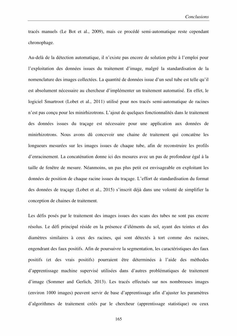
Conclusions

165

tracés manuels (Le Bot et al., 2009), mais ce procédé semi-automatique reste cependant

chronophage.

Au-delà de la détection automatique, il n’existe pas encore de solution prête à l’emploi pour

l’exploitation des données issues du traitement d’image, malgré la standardisation de la

nomenclature des images collectées. La quantité de données issue d’un seul tube est telle qu’il

est absolument nécessaire au chercheur d’implémenter un traitement automatisé. En effet, le

logiciel Smartroot (Lobet et al., 2011) utilisé pour nos tracés semi-automatique de racines

n’est pas conçu pour les minirhizotrons. L’ajout de quelques fonctionnalités dans le traitement

des données issues du traçage est nécessaire pour une application aux données de

minirhizotrons. Nous avons dû concevoir une chaine de traitement qui concatène les

longueurs mesurées sur les images issues de chaque tube, afin de reconstruire les profils

d’enracinement. La concaténation donne ici des mesures avec un pas de profondeur égal à la

taille de fenêtre de mesure. Néanmoins, un pas plus petit est envisageable en exploitant les

données de position de chaque racine issues du traçage. L’effort de standardisation du format

des données de traçage (Lobet et al., 2015) s’inscrit déjà dans une volonté de simplifier la

conception de chaines de traitement.

Les défis posés par le traitement des images issues des scans des tubes ne sont pas encore

résolus. Le défi principal réside en la présence d’éléments du sol, ayant des teintes et des

diamètres similaires à ceux des racines, qui sont détectés à tort comme des racines,

engendrant des faux positifs. Afin de poursuivre la segmentation, les caractéristiques des faux

positifs (et des vrais positifs) pourraient être déterminées à l’aide des méthodes

d’apprentissage machine supervisé utilisées dans d’autres problématiques de traitement

d’image (Sommer and Gerlich, 2013). Les tracés effectués sur nos nombreuses images

(environ 1000 images) peuvent servir de base d’apprentissage afin d’ajuster les paramètres

d’algorithmes de traitement créés par le chercheur (apprentissage statistique) ou ceux

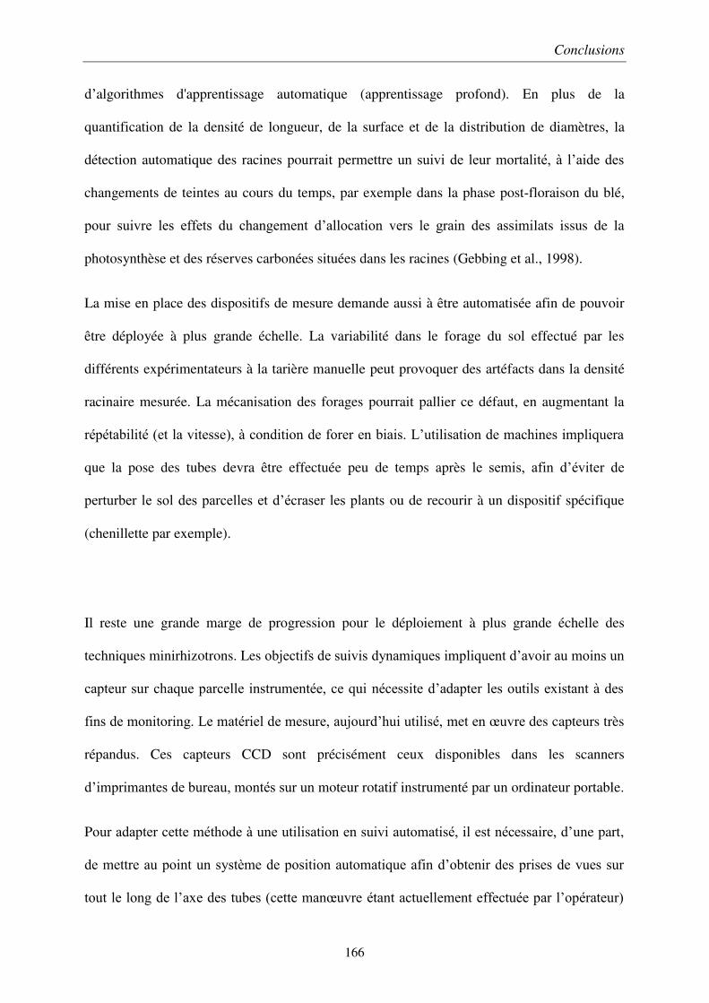
Conclusions

166

d’algorithmes d'apprentissage automatique (apprentissage profond). En plus de la

quantification de la densité de longueur, de la surface et de la distribution de diamètres, la

détection automatique des racines pourrait permettre un suivi de leur mortalité, à l’aide des

changements de teintes au cours du temps, par exemple dans la phase post-floraison du blé,

pour suivre les effets du changement d’allocation vers le grain des assimilats issus de la

photosynthèse et des réserves carbonées situées dans les racines (Gebbing et al., 1998).

La mise en place des dispositifs de mesure demande aussi à être automatisée afin de pouvoir

être déployée à plus grande échelle. La variabilité dans le forage du sol effectué par les

différents expérimentateurs à la tarière manuelle peut provoquer des artéfacts dans la densité

racinaire mesurée. La mécanisation des forages pourrait pallier ce défaut, en augmentant la

répétabilité (et la vitesse), à condition de forer en biais. L’utilisation de machines impliquera

que la pose des tubes devra être effectuée peu de temps après le semis, afin d’éviter de

perturber le sol des parcelles et d’écraser les plants ou de recourir à un dispositif spécifique

(chenillette par exemple).

Il reste une grande marge de progression pour le déploiement à plus grande échelle des

techniques minirhizotrons. Les objectifs de suivis dynamiques impliquent d’avoir au moins un

capteur sur chaque parcelle instrumentée, ce qui nécessite d’adapter les outils existant à des

fins de monitoring. Le matériel de mesure, aujourd’hui utilisé, met en œuvre des capteurs très

répandus. Ces capteurs CCD sont précisément ceux disponibles dans les scanners

d’imprimantes de bureau, montés sur un moteur rotatif instrumenté par un ordinateur portable.

Pour adapter cette méthode à une utilisation en suivi automatisé, il est nécessaire, d’une part,

de mettre au point un système de position automatique afin d’obtenir des prises de vues sur

tout le long de l’axe des tubes (cette manœuvre étant actuellement effectuée par l’opérateur)

Conclusions

167

et d’autre part, de doter les capteurs minirhizotrons d’une capacité de communication des

données. Ces évolutions semblent possibles, compte tenu du développement des objets

connectés et de l’automatisation, à l’instar des plateformes de réseaux de capteurs mesurant

l’humidité du sol et la température de l’air et du sol (Bitella et al., 2014), développés pour

l’agriculture de précision.

Les données des profils racinaires sont riches en informations et ne forment pas un

paramètre/indice unique. Une approche similaire à celle utilisée dans le domaine du

phénotypage des parties aériennes pourrait simplifier l’utilisation de ces données, en réduisant

leur dimension, autrement dit en réduisant un vecteur de points qui caractérisent un profil

racinaire en un scalaire ou un indice. Ces profils sont l’équivalent des spectres issus de

l’imagerie des parties aériennes. La réduction de tels profils à quelques traits caractéristiques

simplifierait leur utilisation en sélection végétale.

L’observation des profils racinaires indique que la distribution en profondeur des racines, et

pas seulement leur quantité totale, est un paramètre important.

En considérant la profondeur médiane de densité racinaire observée en minirhizotrons

(autrement dit, la profondeur à partir de laquelle 50% des racines ont été observées) une

analyse de variance (ANOVA) fait apparaître un effet lié à la variété et à son interaction avec

le traitement azoté, invisible en ne considérant que la densité moyenne de racines (Tableau

1 ). Par exemple, l’essai 2015 montre que certaines variétés résistent mieux à la sécheresse,

notamment lorsqu’elles sont privées d’apport en azote.

Ici très peu de réplications sont considérées. Avec une plus grande variété d’enracinements et

de réplications, il serait possible d’utiliser des paramètres/descripteurs qui pourraient décrire

les aspects d’amplitude, de localisation, d’asymétrie des profils d’enracinement, à l’image des

techniques de statistique descriptive.

Conclusions

168

L’extension de minirhizotrons à un contexte de monitoring à plus grande échelle, pour des

applications de phénotypage « moyen débit » semble donc envisageable. Une fois les

algorithmes de traitement d’image conçus, les traits globaux des systèmes racinaires seraient

plus aisés d’accès. La pertinence des traits visés dans un contexte de sélection donné

(résistance à la sécheresse, réduction/augmentation de la taille des systèmes racinaires) pourra

être évaluée à partir de modèles de culture incluant une modélisation du compartiment

racinaire. Toutefois, les structures les plus fines des systèmes racinaires, par exemple les

mycorhizes et poils racinaires, restent difficiles d’accès et la biomasse n’est estimée qu’à

travers le volume des racines. Pour l’heure, aucun moyen de mesure adapté à une utilisation

au champ ne permet la mesure simultanée de la masse et de la morphologie du système

racinaire. Néanmoins, des prélèvements destructifs peuvent être complémentaires des mesures

minirhizotron. Les prélèvements destructifs permettent de mesurer la masse linéique des

racines et l’enracinement superficiel, pendant que les minirhizotrons donnent accès aux

couches profondes en apportant un aspect dynamique. De plus une calibration à une

profondeur donnée entre la masse racinaire obtenue par prélèvement destructif et le volume

des racines mesuré au minirhizotron permet d’estimer la masse des racines situées en couches

profondes.

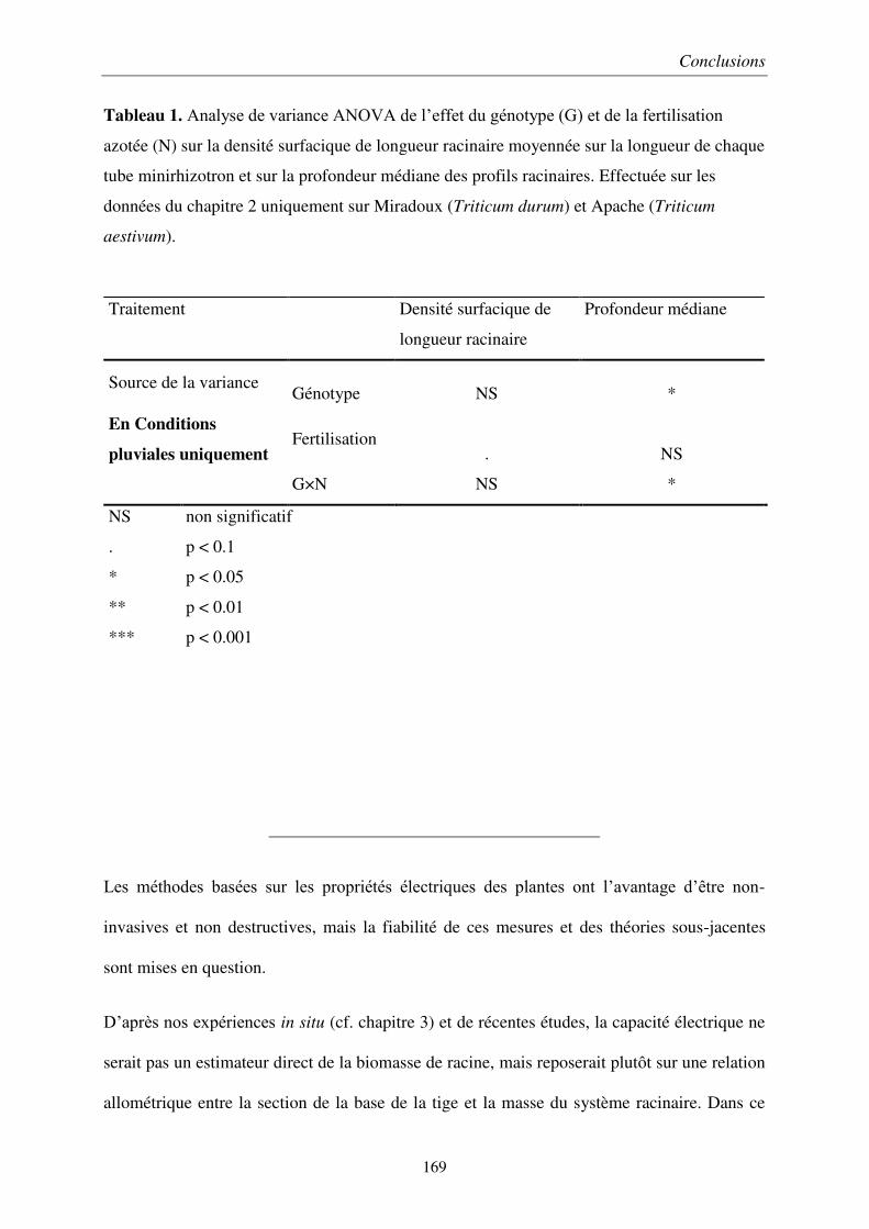
Conclusions

169

Tableau 1. Analyse de variance ANOVA de l’effet du génotype (G) et de la fertilisation

azotée (N) sur la densité surfacique de longueur racinaire moyennée sur la longueur de chaque

tube minirhizotron et sur la profondeur médiane des profils racinaires. Effectuée sur les

données du chapitre 2 uniquement sur Miradoux (Triticum durum) et Apache (Triticum

aestivum).

Les méthodes basées sur les propriétés électriques des plantes ont l’avantage d’être non-

invasives et non destructives, mais la fiabilité de ces mesures et des théories sous-jacentes

sont mises en question.

D’après nos expériences in situ (cf. chapitre 3) et de récentes études, la capacité électrique ne

serait pas un estimateur direct de la biomasse de racine, mais reposerait plutôt sur une relation

allométrique entre la section de la base de la tige et la masse du système racinaire. Dans ce

Traitement Densité surfacique de

longueur racinaire

Profondeur médiane

Source de la variance Génotype NS *

En Conditions

pluviales uniquement Fertilisation

. NS

G×N NS *

NS non significatif

. p < 0.1

* p < 0.05

** p < 0.01

*** p < 0.001

Conclusions

170

cas, la relation allométrique reliant la capacité électrique à la biomasse racinaire semble être

variable in situ, en particulier une fois le stade végétatif dépassé. Dans nos mesures, l’absence

de relation entre la capacité électrique et la masse racinaire aux stades reproductifs rend alors

discutable l’usage de la capacité électrique pour prédire la biomasse racinaire. Ce type de

résultats remet en cause la fiabilité de la théorie principale élaborée par Dalton (1995) à partir

des résultats empiriques de Chloupek (1977). Toutefois, en exploitant la théorie formulée par

Dietrich (2012), dans le chapitre 3, nous montrons que la réactance pourrait être un estimateur

de la biomasse racinaire, principalement dans les couches superficielles du sol, lorsque

l’humidité du sol est faible, et que le diamètre des racines a une assez faible variance. De plus,

les résultats complémentaires du chapitre 3 indiquent que la variabilité intra-cultivar de la

réactance est suffisamment faible pour que l’on puisse identifier des effets liés au génotype.

Le développement des techniques basées sur l’impédance nous semble limité actuellement en

raison de l’absence d’un modèle électrique complet d’une plante en situation de culture.

L’impédance des différents tissus composant la plante n’est pas déterminée, à l’instar du

passage exact du courant dans un sol hétérogène partiellement asséché. Une mesure du

spectre électrique des tissus racinaires de la plante ajouterait à l’élaboration et la

compréhension d’un modèle électrique équivalent. Ce dernier pourrait permettre d’identifier

les composantes du spectre les plus en lien avec la masse racinaire. En ayant en complément

un modèle de variation d’impédance (principalement de résistivité) des sols en fonction de

leur teneur en eau, il sera possible de définir la plage d’humidité dans laquelle le contraste

électrique est suffisant pour prédire la biomasse racinaire. Les développements sur

l’utilisation du spectre électrique fait partie des objectifs du chapitre 1, à travers l’étude de

l’effet de la fréquence sur la corrélation entre biomasse racinaire et capacité (et les autres

variables électriques). Cependant les mesures ont été effectuées sur des plantes dans un sol

humide, cette configuration donnant un poids primordial à la partie proximale des racines à

Conclusions

171

cause de la forte conductivité du sol. Les spectres électriques ne pourraient concerner alors

principalement les tissus de la base de la tige et la partie proximale du système racinaire. La

variation de la qualité de l’estimation de la masse racinaire en fonction de la fréquence du

courant proviendrait alors pour partie de la variation de la relation allométrique liant la section

de la tige et des racines à sa base et la capacité mais également du fait, dans des plages de

fréquences où le sol contribue plus fortement à la capacité totale, d’une moindre sensibilité de

la relation section de tige et racines à la base – capacité électrique. Malgré ces limitations

relatives aux méthodes expérimentales et à la théorie utilisée, plusieurs études ont eu pour

objet l’application de la technique (en utilisant la capacité électrique) à des fins de monitoring

ou de sélections. Récemment, la capacité électrique a été utilisée pour le suivi de la biomasse

racinaire de plants de soja, cultivés en pots, pour suivre l’effet du stress hydrique sur la

dynamique de croissance du système racinaire (Cseresnyés et al., 2016). Dans un cadre de

sélection variétale, une analyse de variance (Chloupek et al., 2006) sur 158 génotypes d’orges

(Hordeum vulgare), avec seulement 3 répétitions de mesures de capacité électrique — jugée

dans l’étude comme un estimateur fiable de la biomasse racinaire — par génotype a permis de

déterminer des locus de caractères quantitatifs (QTL) liés aux mesures de capacité électrique.

Il ressort que les QTLs détectés par ces mesures de capacité sont des zones du génome

associées à des traits aériens (notamment nanisme et rapport grain sur paille). De même, la

sélection sur ce même critère de capacité électrique (Cp), montre que le caractère lié à des

valeurs de Cp élevées chez les plantes est transmissible de façon héréditaire chez le blé

(Heřmanská et al., 2015) et l’orge (Svačina et al., 2014). Les auteurs constatent que les

lignées à haute capacité électrique possèdent aussi de meilleur rendement en conditions

optimales.

Ces expérimentations sont effectuées systématiquement dans des sols humides. Ceci implique

que la capacité électrique est un estimateur du diamètre de la tige à sa base ou de la section

Conclusions

172

des racines à l’interface sol air, et non directement de la biomasse des racines d’une plante

(Dietrich et al., 2012). Donc les traits transmis, et les QTLs détectés pourraient être en lien

avec le diamètre de la tige ou la partie proximale du système racinaire. La corrélation entre les

rendements des plants de blé et les mesures de capacité pourraient s’expliquer par l’inter-

corrélation de plusieurs traits. Chez le blé, la masse des parties aériennes est corrélée au

rendement (Reynolds et al., 1999), et plus largement il existe une relation allométrique entre

diamètre de la tige et biomasse des plantes (Niklas, 1993).

À l’inverse des mesures de capacité électrique, la réactance est un estimateur direct de la

longueur racinaire, et par extension de la biomasse. L’application au champ de la réactance en

tant qu’estimateur de biomasse, requiert des informations sur l’état d’humidité du sol, et son

efficacité in situ est dépendante des conditions climatiques en l’absence de mise à l’abri de la

pluie. Bien que la technique actuelle ne soit pas automatisée, plusieurs plantes pourraient être

suivies en multiplexant les mesures d’impédance sur des plantes localisées autour d’un pont

de mesure RLC et des (micro)parcelles expérimentales pourraient être équipées de ce type de

système au même titre que des capteurs environnementaux.

Dans le premier chapitre de la thèse, nous avons identifié quelques aspects expérimentaux

pratiques de la méthode basée sur l’impédance — il n’est pas nécessaire d’utiliser des

aiguilles pour transmettre le courant — et nous avons évalué l’effet des sols de classes

texturales différentes sur l’estimation de la biomasse racinaire par mesure électrique. Ces

développements sur la méthodologie contribuent à son extension comme moyen de mesure à

plus grande échelle. Le matériel de mesure électrique nécessaire, un pont RLC portable

programmable tel le Red Pitaya, est actuellement disponible à un coût relativement faible.

Puisqu’un système de mise en contact électrique mobile est difficilement concevable,

l’utilisation d’un réseau de capteurs fixes au sol est à préférer à l’embarquement de capteurs

dans un véhicule de phénotypage.

Conclusions

173

D’après nos résultats, la réactance est un proxy de la biomasse racinaire applicable

uniquement en conditions de sécheresse, mesurant plutôt la partie superficielle du système

racinaire dans la zone sèche. À première vue, la réactance parait inadaptée dans les études sur

la résistance à la sécheresse du blé, puisque celles-ci se focalisent souvent sur l'acquisition par

le système racinaire de l'humidité et des nutriments situés plus en profondeur (Manschadi et

al., 2010). Cependant, chez le maïs, il apparait qu’une réduction de la masse racinaire

superficielle pourrait induire une résistance à la sécheresse (Zhu et al., 2005). Ce type de

mécanisme pourrait être présent chez le blé, faisant ainsi de la réactance un outil intéressant

de sélection des cultures pour la résistance à la sécheresse. La technique pourrait être

applicable aux études utilisant des abris anti pluie pour simuler des sécheresses ou aux régions

touchées par la sécheresse, telles que les zones méditerranéennes et tropicales semi-arides.

Au final, les mesures de propriétés des systèmes racinaires en plein champ par des méthodes

indirectes ne peuvent pas s’affranchir d’un effet sol. En effet, dès que l’on utilise un signal

injecté : propagation d’onde (ondes électromagnétiques, comme le géoradar, ou mécaniques,

comme en sismique) ou une conduction (conductivité électrique en tomographie de résistivité

électrique, ou mesures capacitives…), le sol va fortement conditionner le signal transmis et

donc le contraste et la résolution des mesures en relation avec les racines. Ainsi, l’humidité du

sol joue un rôle prépondérant dans la détection des racines à l’aide d’ondes

électromagnétiques ou avec les méthodes capacitives et il en est de même pour la teneur en

argile des sols. À l’avenir, pour la quantification in situ des racines, il serait nécessaire

d’avoir une caractérisation plus fine des propriétés physiques des sols afin d’évaluer

l’influence du sol sur l’emploi des techniques électriques indirectes et ainsi mieux définir les

situations propices à la détection de racines.

Conclusions

174

Les mesures invasives, mais plus directes, étant moins sujettes à l’hétérogénéité physique du

sol semblent pour leur part plus à même de contribuer rapidement à la sélection variétale. Aux

stades jeunes de développement, la croissance et la morphologie des systèmes racinaires sont

en train de devenir accessibles avec les serres automatisées et des phénotypes racinaires

peuvent déjà être testés dans ces conditions. Le test au champ de ces phénotypes en nombre

plus réduit, sur des durées plus longues, en situations de multi-contraintes pour la plante et sur

des stades plus avancés pourra s’enrichir des données racinaires avec ces méthodes plus

invasives, telles que les minirhizotrons. Cependant, ceci serait à pondérer en fonction d’une

possible faible héritabilité des traits racinaires, où de multiples gènes pourraient entrer en jeu,

nécessitant un débit expérimental (en nombre d’individus plantes et parcelles) pour identifier

les gènes liés aux traits d’intérêts dépassant les possibilités actuelles des méthodes invasives.

Annexes

175

Annexes

Annexes

176

Annexe au chapitre 1

Additional file 1: Table S1 (.doc). Sensitivity score details and linear regression parameters

between root dry mass and each electrical variable. The table lists the maximum

determination frequency (fmax, Hz), sensitivity scores, maximum of coefficient of

determination with root dry mass (r2max), y-intercept of the linear regression (in standard unit

of the related electrical variable) and slope (in standard unit of the related electrical variable

per g) for parallel capacitance (Cp), serial capacitance (Cs), parallel resistance (Rp), serial

resistance (Rs), conductance magnitude (G), impedance magnitude (Z), reactance (X) and

impedance phase angle (θ) in 2T, 3T and 4T configurations, on average for 3 soil types.

   

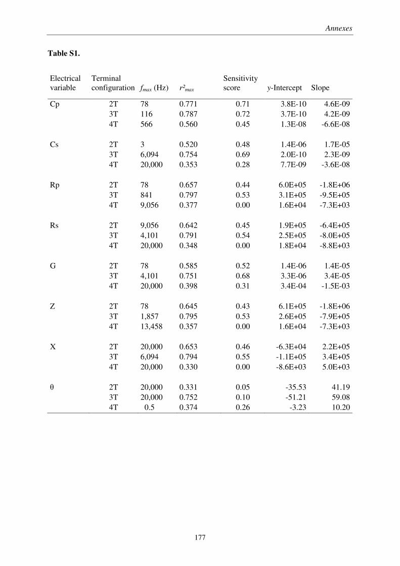
Annexes

177

Table S1.

Electrical variable

Terminal configuration fmax (Hz) r²max

Sensitivity score y-Intercept Slope

Cp 2T 78 0.771 0.71 3.8E-10 4.6E-09 3T 116 0.787 0.72 3.7E-10 4.2E-09 4T 566 0.560 0.45 1.3E-08 -6.6E-08 Cs 2T 3 0.520 0.48 1.4E-06 1.7E-05 3T 6,094 0.754 0.69 2.0E-10 2.3E-09 4T 20,000 0.353 0.28 7.7E-09 -3.6E-08 Rp 2T 78 0.657 0.44 6.0E+05 -1.8E+06 3T 841 0.797 0.53 3.1E+05 -9.5E+05 4T 9,056 0.377 0.00 1.6E+04 -7.3E+03 Rs 2T 9,056 0.642 0.45 1.9E+05 -6.4E+05 3T 4,101 0.791 0.54 2.5E+05 -8.0E+05 4T 20,000 0.348 0.00 1.8E+04 -8.8E+03 G 2T 78 0.585 0.52 1.4E-06 1.4E-05 3T 4,101 0.751 0.68 3.3E-06 3.4E-05 4T 20,000 0.398 0.31 3.4E-04 -1.5E-03 Z 2T 78 0.645 0.43 6.1E+05 -1.8E+06 3T 1,857 0.795 0.53 2.6E+05 -7.9E+05 4T 13,458 0.357 0.00 1.6E+04 -7.3E+03 X 2T 20,000 0.653 0.46 -6.3E+04 2.2E+05 3T 6,094 0.794 0.55 -1.1E+05 3.4E+05 4T 20,000 0.330 0.00 -8.6E+03 5.0E+03 θ 2T 20,000 0.331 0.05 -35.53 41.19 3T 20,000 0.752 0.10 -51.21 59.08 4T 0.5 0.374 0.26 -3.23 10.20

   

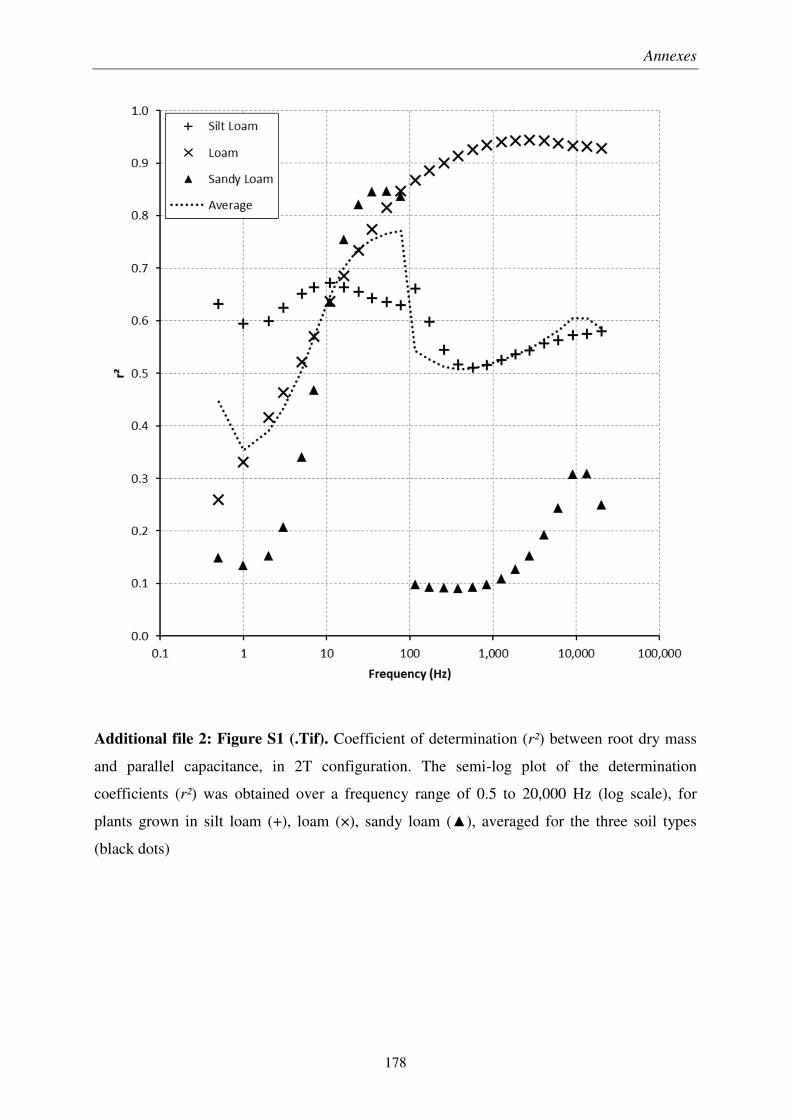
Annexes

178

Additional file 2: Figure S1 (.Tif). Coefficient of determination (r²) between root dry mass

and parallel capacitance, in 2T configuration. The semi-log plot of the determination

coefficients (r²) was obtained over a frequency range of 0.5 to 20,000 Hz (log scale), for

plants grown in silt loam (+), loam (×), sandy loam (▲), averaged for the three soil types

(black dots)

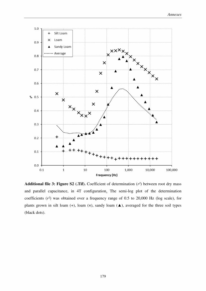
Annexes

179

Additional file 3: Figure S2 (.Tif). Coefficient of determination (r²) between root dry mass

and parallel capacitance, in 4T configuration. The semi-log plot of the determination

coefficients (r²) was obtained over a frequency range of 0.5 to 20,000 Hz (log scale), for

plants grown in silt loam (+), loam (×), sandy loam (▲), averaged for the three soil types

(black dots).

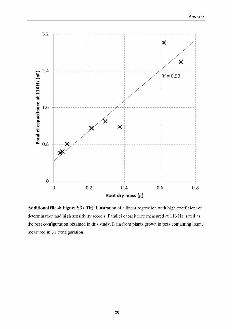
Annexes

180

Additional file 4: Figure S3 (.Tif). Illustration of a linear regression with high coefficient of

determination and high sensitivity score s. Parallel capacitance measured at 116 Hz, rated as

the best configuration obtained in this study. Data from plants grown in pots containing loam,

measured in 3T configuration.

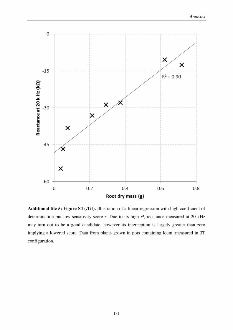
Annexes

181

Additional file 5: Figure S4 (.Tif). Illustration of a linear regression with high coefficient of

determination but low sensitivity score s. Due to its high r², reactance measured at 20 kHz

may turn out to be a good candidate, however its interception is largely greater than zero

implying a lowered score. Data from plants grown in pots containing loam, measured in 3T

configuration.

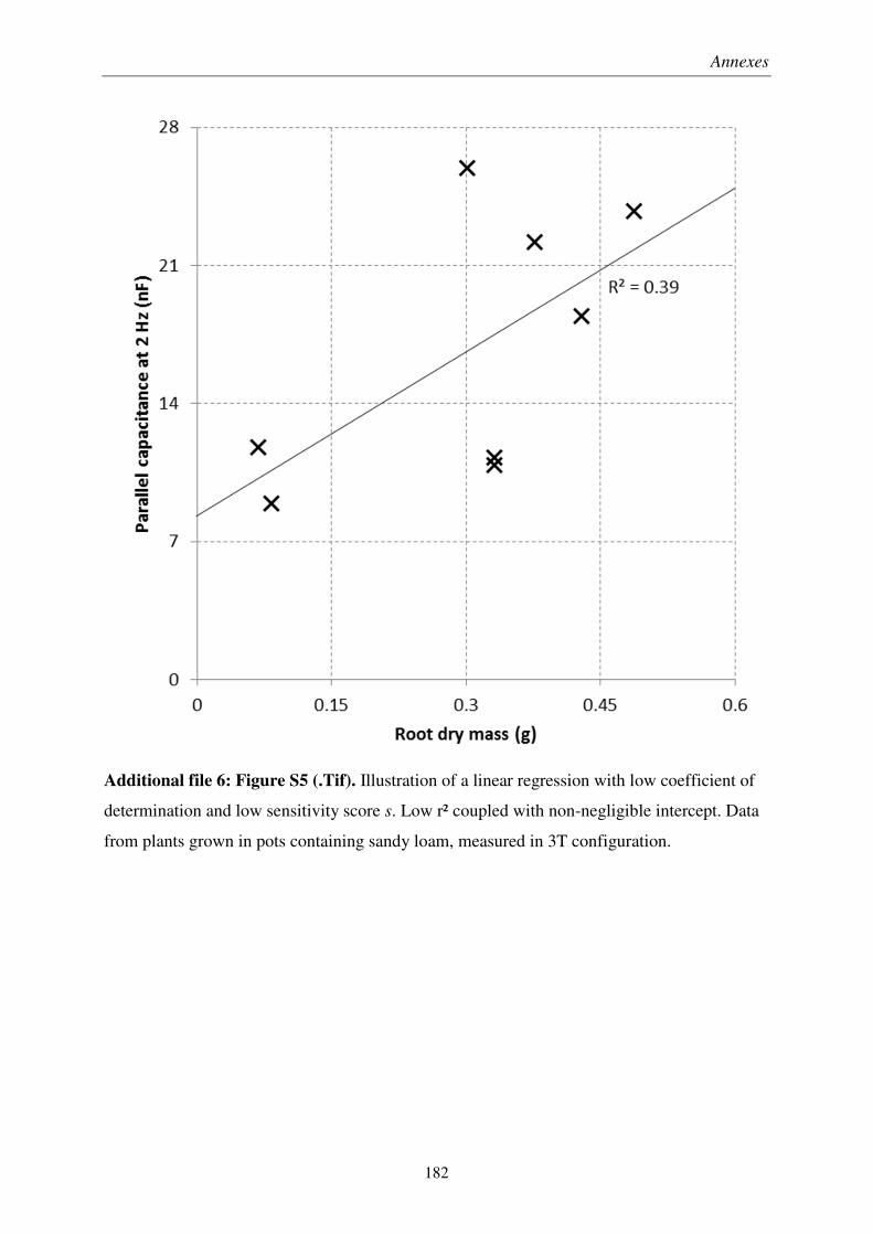
Annexes

182

Additional file 6: Figure S5 (.Tif). Illustration of a linear regression with low coefficient of

determination and low sensitivity score s. Low r² coupled with non-negligible intercept. Data

from plants grown in pots containing sandy loam, measured in 3T configuration.

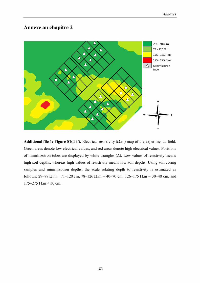
Annexes

183

Annexe au chapitre 2

Additional file 1: Figure S1(.Tif). Electrical resistivity (Ω.m) map of the experimental field.

Green areas denote low electrical values, and red areas denote high electrical values. Positions

of minirhizotron tubes are displayed by white triangles (Δ). Low values of resistivity means

high soil depths, whereas high values of resistivity means low soil depths. Using soil coring

samples and minirhizotron depths, the scale relating depth to resistivity is estimated as

follows: 29–78 Ω.m = 71–120 cm, 78–126 Ω.m = 40–70 cm, 126–175 Ω.m = 30–40 cm, and

175–275 Ω.m < 30 cm.

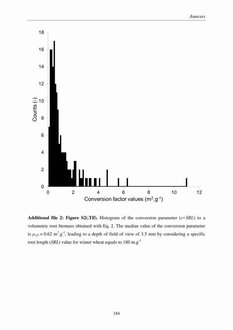
Annexes

184

Additional file 2: Figure S2(.Tif). Histogram of the conversion parameter (ε×SRL) to a

volumetric root biomass obtained with Eq. 2. The median value of the conversion parameter

is μ1/2 = 0.62 m2.g-1, leading to a depth of field of view of 3.5 mm by considering a specific

root length (SRL) value for winter wheat equals to 180 m.g-1

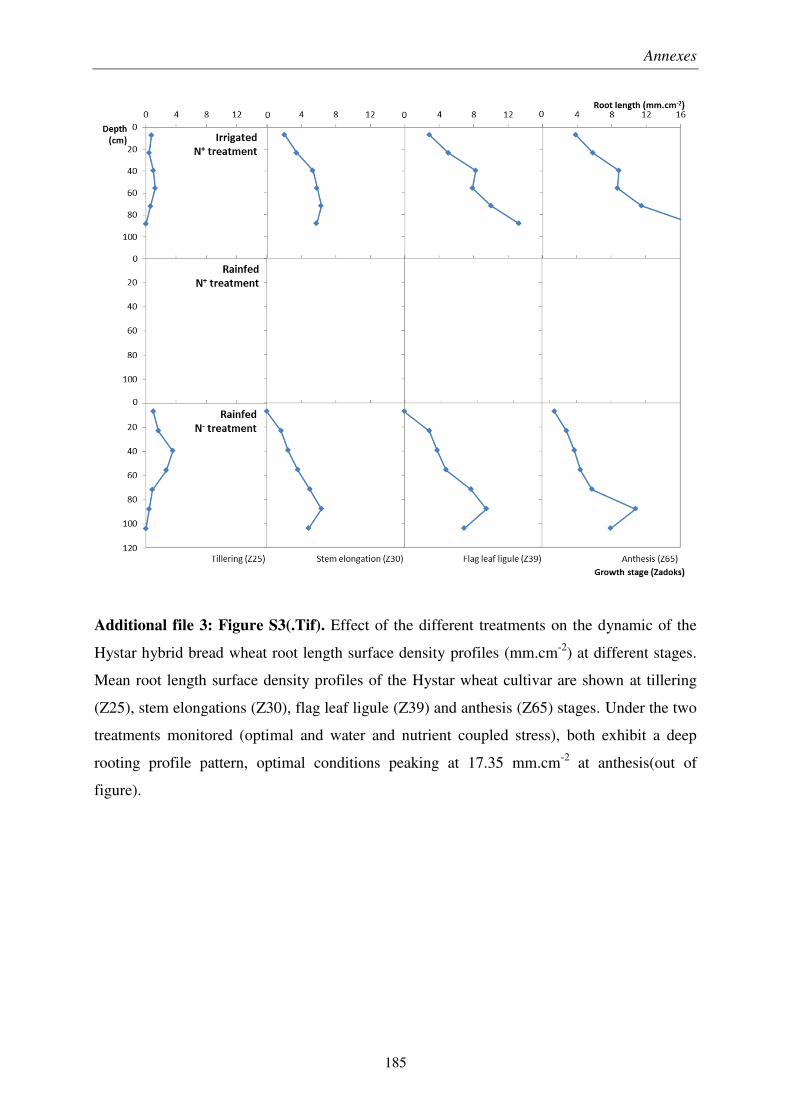
Annexes

185

Additional file 3: Figure S3(.Tif). Effect of the different treatments on the dynamic of the

Hystar hybrid bread wheat root length surface density profiles (mm.cm-2) at different stages.

Mean root length surface density profiles of the Hystar wheat cultivar are shown at tillering

(Z25), stem elongations (Z30), flag leaf ligule (Z39) and anthesis (Z65) stages. Under the two

treatments monitored (optimal and water and nutrient coupled stress), both exhibit a deep

rooting profile pattern, optimal conditions peaking at 17.35 mm.cm-2 at anthesis(out of

figure).

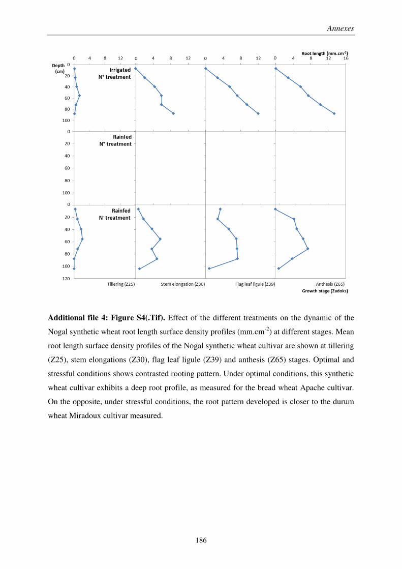
Annexes

186

 

Additional file 4: Figure S4(.Tif). Effect of the different treatments on the dynamic of the

Nogal synthetic wheat root length surface density profiles (mm.cm-2) at different stages. Mean

root length surface density profiles of the Nogal synthetic wheat cultivar are shown at tillering

(Z25), stem elongations (Z30), flag leaf ligule (Z39) and anthesis (Z65) stages. Optimal and

stressful conditions shows contrasted rooting pattern. Under optimal conditions, this synthetic

wheat cultivar exhibits a deep root profile, as measured for the bread wheat Apache cultivar.

On the opposite, under stressful conditions, the root pattern developed is closer to the durum

wheat Miradoux cultivar measured.

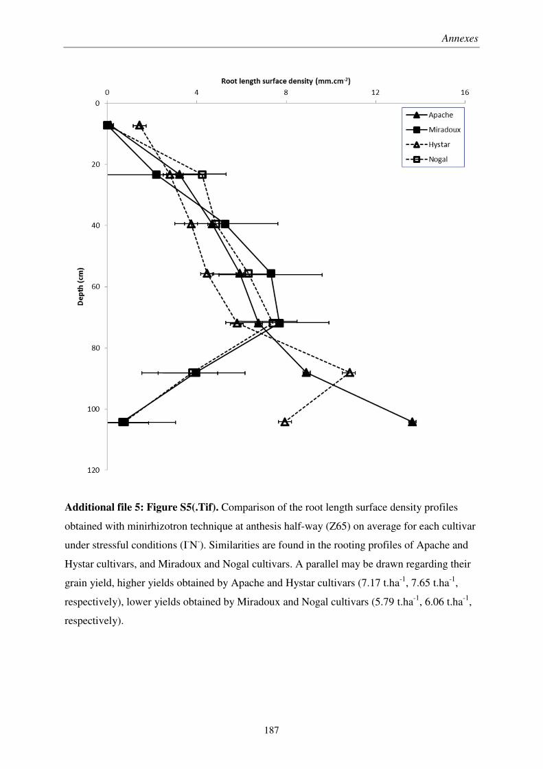
Annexes

187

 

Additional file 5: Figure S5(.Tif). Comparison of the root length surface density profiles

obtained with minirhizotron technique at anthesis half-way (Z65) on average for each cultivar

under stressful conditions (I-N-). Similarities are found in the rooting profiles of Apache and

Hystar cultivars, and Miradoux and Nogal cultivars. A parallel may be drawn regarding their

grain yield, higher yields obtained by Apache and Hystar cultivars (7.17 t.ha-1, 7.65 t.ha-1,

respectively), lower yields obtained by Miradoux and Nogal cultivars (5.79 t.ha-1, 6.06 t.ha-1,

respectively).

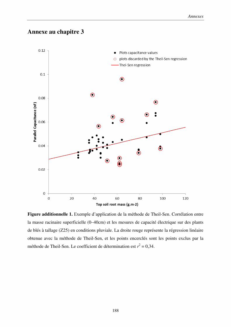
Annexes

188

Annexe au chapitre 3

Figure additionnelle 1. Exemple d’application de la méthode de Theil-Sen. Corrélation entre

la masse racinaire superficielle (0–40cm) et les mesures de capacité électrique sur des plants

de blés à tallage (Z25) en conditions pluviale. La droite rouge représente la régression linéaire

obtenue avec la méthode de Theil-Sen, et les points encerclés sont les points exclus par la

méthode de Theil-Sen. Le coefficient de détermination est r2 = 0,34.

 

Références

Références

190

Alexandratos N, Bruinsma J. 2012. World agriculture towards 2030/2050: the 2012 revision. ESA Working paper Rome, FAO. Allard V, Martre P, Le Gouis J. 2013. Genetic variability in biomass allocation to roots in wheat is mainly related to crop tillering dynamics and nitrogen status. European Journal of Agronomy 46, 68–76. Amato M, Basso B, Celano G, Bitella G, Morelli G, Rossi R. 2008. In situ detection of tree root distribution and biomass by multi-electrode resistivity imaging. Tree physiology 28, 1441–1448. Araus JL, Cairns JE. 2014. Field high-throughput phenotyping: the new crop breeding frontier. Trends in Plant Science 19, 52–61. Araus JL, Slafer GA, Reynolds MP, Royo C. 2002. Plant breeding and drought in C3 cereals: what should we breed for? Annals of Botany 89, 925–940. Asseng S, Ewert F, Martre P, et al. 2014. Rising temperatures reduce global wheat production. Nature Climate Change 5, 143–147. Atkinson D. 1985. Spatial and temporal aspects of root distribution as indicated by the use of a root observation laboratory. Special publications series of the British Ecological Society. Atkinson D. 2000. Root characteristics: why and what to measure. In: Smit AL,, In: Bengough AG,, In: Engels C,, In: van Noordwijk M,, In: Pellerin S,, In: van de Geijn SC, eds. Root methods: a handbook. Springer-Verlag Berlin Heidelberg, 1–32. Attia Al Hagrey S. 2007. Geophysical imaging of root-zone, trunk, and moistureheterogeneity. J Exp Bot 58, 839–54. Aulen M, Shipley B. 2012. Non-destructive estimation of root mass using electrical capacitance on ten herbaceous species. Plant and Soil 355, 41–49. Barraclough PB, Kuhlmann H, Weir AH. 1989. The Effects of Prolonged Drought and Nitrogen Fertilizer on Root and Shoot Growth and Water Uptake by Winter Wheat. Journal of Agronomy and Crop Science 163, 352–360. Barraclough PB, Leigh RA. 1984. The growth and activity of winter wheat roots in the field: the effect of sowing date and soil type on root growth of high-yielding crops. The Journal of Agricultural Science 103, 59–74. Barraclough PB, Weir AH, Kulhmann H. 1991. Factors Affecting the Growth and Distribution of Winter Wheat Roots Under Uk Field Conditions. In: McMichael BL,, In: Persson H, eds. Plant Roots and their Environment. Developments in Agricultural and Managed Forest Ecology. Elsevier, 410–417. van Beem J, Smith ME, Zobel RW. 1998. Estimating root mass in maize using a portable capacitance meter. Agronomy Journal 90, 566–570. Berhongaray G, King JS, Janssens IA, Ceulemans R. 2013. An optimized fine root sampling methodology balancing accuracy and time investment. Plant and Soil 366, 351–361. Bertholdsson N-O, Brantestam AK. 2009. A century of Nordic barley breeding — effects on early vigour root and shoot growth, straw length, harvest index and grain weight. European journal of agronomy 30, 266–274. Bitella G, Rossi R, Bochicchio R, Perniola M, Amato M. 2014. A Novel Low-Cost Open-Hardware Platform for Monitoring Soil Water Content and Multiple Soil-Air-Vegetation Parameters. Sensors 14, 19639–19659. Bock CH, Poole GH, Parker PE, Gottwald TR. 2010. Plant Disease Severity Estimated

Références

191

Visually, by Digital Photography and Image Analysis, and by Hyperspectral Imaging. Critical Reviews in Plant Sciences 29, 59–107. Borch K, Bouma TJ, Lynch JP, Brown KM. 1999. Ethylene: a regulator of root architectural responses to soil phosphorus availability. Plant, Cell & Environment 22, 425–431. Borlaug NE. Finlay KW, Shepherd KW. 1968. Wheat breeding and its impact on world food supply. Canberra: Australian Academy of Science, 1–36. Box JE, Smucker AJM, Ritchie JT. 1989. Minirhizotron installation techniques for investigating root responses to drought and oxygen stresses. Soil Science Society of America Journal 53, 115–118. Brisson N, Gate P, Gouache D, Charmet G, Oury F-X, Huard F. 2010. Why are wheat yields stagnating in Europe? A comprehensive data analysis for France. Field Crops Research 119, 201–212. Brunelle T, Dumas P, Souty F, Dorin B, Nadaud F. 2015. Evaluating the impact of rising fertilizer prices on crop yields. Agricultural Economics 46, 653–666. Bucksch A, Burridge J, York LM, Das A, Nord E, Weitz JS, Lynch JP. 2014. Image-Based High-Throughput Field Phenotyping of Crop Roots. PLANT PHYSIOLOGY 166, 470–486. Cao Y, Repo T, Silvennoinen R, Lehto T, Pelkonen P. 2011. Analysis of the willow root system by electrical impedance spectroscopy. J Exp Bot 62, 351–8. Carberry PS, Liang W, Twomlow S, Holzworth DP, Dimes JP, McClelland T, Huth NI, Chen F, Hochman Z, Keating BA. 2013. Scope for improved eco-efficiency varies among diverse cropping systems. Proceedings of the National Academy of Sciences 110, 8381–8386. Cermak J, Radek U, Stranek Z, Koller J, Aubrecht L. 2006. Electrical measurement of tree root absorbing surfaces by the earth impedance method: 2. Verification based on allometric relationships and root severing experiments. Tree Physiology 26, 1113–1121. Chaudhuri UN, Kirkham MB, Kanemasu ET. 1990. Root growth of winter wheat under elevated carbon dioxide and drought. Crop Science 30, 853–857. Chloupek O. 1972. The relationship between electric capacitance and some other parameters of plant roots. Biologia Plantarum 14, 227–230. Chloupek O. 1977. Evaluation of the size of a plant’s root system using its electrical capacitance. Plant and Soil 48, 525–532. Chloupek O, Dostál V, Středa T, Psota V, Dvořáčková O. 2010. Drought tolerance of barley varieties in relation to their root system size. Plant Breeding 129, 630–636. Chloupek O, Forster BP, Thomas WT. 2006. The effect of semi-dwarf genes on root system size in field-grown barley. Theoretical and Applied Genetics 112, 779–786. Christidis N, Jones GS, Stott PA. 2014. Dramatically increasing chance of extremely hot summers since the 2003 European heatwave. Nature Climate Change 5, 46–50. Christopher JT, Manschadi AM, Hammer GL, Borrell AK. 2008. Developmental and physiological traits associated with high yield and stay-green phenotype in wheat. Australian Journal of Agricultural Research 59, 354. Clark RT, MacCurdy RB, Jung JK, Shaff JE, McCouch SR, Aneshansley DJ, Kochian LV. 2011. Three-Dimensional Root Phenotyping with a Novel Imaging and Software Platform. PLANT PHYSIOLOGY 156, 455–465.

Références

192

Colombi T, Kirchgessner N, Marié CAL, York LM, Lynch JP, Hund A. 2015. Next generation shovelomics: set up a tent and REST. Plant and Soil 388, 1–20. Comar A, Burger P, de Solan B, Baret F, Daumard F, Hanocq J-F. 2012. A semi-automatic system for high throughput phenotyping wheat cultivars in-field conditions: description and first results. Functional Plant Biology 39, 914–924. Cordell D, Drangert J-O, White S. 2009. The story of phosphorus: Global food security and food for thought. Global Environmental Change 19, 292–305. Coumou D, Rahmstorf S. 2012. A decade of weather extremes. Nature Climate Change. Cseresnyés I, Rajkai K, Takács T. 2016. Indirect monitoring of root activity in soybean cultivars under contrasting moisture regimes by measuring electrical capacitance. Acta Physiologiae Plantarum 38. Cseresnyes I, Rajkai K, Vozary E. 2013. Role of phase angle measurement in electrical impedance spectroscopy. International Agrophysics 27, 377–383. Dalton FN. 1995. In-situ root extent measurements by electrical capacitance methods. Plant and Soil 173, 157–165. De Smet I, White PJ, Bengough AG, et al. 2012. Analyzing Lateral Root Development: How to Move Forward. The Plant Cell 24, 15–20. Deak KI, Malamy J. 2005. Osmotic regulation of root system architecture. The Plant Journal 43, 17–28. Devienne-Barret F, Richard-Molard C, Chelle M, Maury O, Ney B. 2006. Ara-Rhizotron: An Effective Culture System to Study Simultaneously Root and Shoot Development of Arabidopsis. Plant and Soil 280, 253–266. Dietrich RC, Bengough AG, Jones HG, White PJ. 2012. A new physical interpretation of plant root capacitance. Journal of Experimental Botany 63, 6149–6159. Dietrich RC, Bengough AG, Jones HG, White PJ. 2013. Can root electrical capacitance be used to predict root mass in soil? Annals of Botany 112, 457–464. Dubach M, Russelle MP. 1995. Reducing the Cost of Estimating Root Turnover with Horizontally Installed Minirhizotrons. Agronomy Journal 87, 258. Eberbach PL, Hoffmann J, Moroni SJ, Wade LJ, Weston LA. 2013. Rhizo-lysimetry: facilities for the simultaneous study of root behaviour and resource use by agricultural crop and pasture systems. Plant methods 9, 3. Eizenberg H. 2005. A New Method for in-situ Monitoring of the Underground Development of Orobanche cumana in Sunflower (Helianthus annuus) with a Mini-rhizotron. Annals of Botany 96, 1137–1140. Ellis T, Murray W, Kavalieris L. 2013a. Electrical capacitance of bean (Vicia faba) root systems was related to tissue density-a test for the Dalton Model. Plant and Soil 366, 575–584. Ellis TW, Murray W, Paul K, Kavalieris L, Brophy J, Williams C, Maass M. 2013b. Electrical capacitance as a rapid and non-invasive indicator of root length. Tree Physiology 33, 3–17. Ephrath JE, Silberbush M, Berliner PR. 1999. Calibration of minirhizotron readings against root length density data obtained from soil cores. Plant and Soil 209, 201–208. Fan J, McConkey B, Wang H, Janzen H. 2016. Root distribution by depth for temperate agricultural crops. Field Crops Research 189, 68–74.

Références

193

FAO of the United Nations. 2014. Crop prospects and food situation. October(No. 3). Rome: FAO. FAO of the United Nations. 2015. World fertilizer trends and outlook to 2018. Rome: Food & Agriculture Organization of United Nations. Fernandes R, G. Leblanc S. 2005. Parametric (modified least squares) and non-parametric (Theil–Sen) linear regressions for predicting biophysical parameters in the presence of measurement errors. Remote Sensing of Environment 95, 303–316. Fiorani F, Schurr U. 2013. Future Scenarios for Plant Phenotyping. Annual Review of Plant Biology 64, 267–291. Fischer RA, Byerlee D, Edmeades G. 2014. Crop yields and global food security. ACIAR: Canberra, ACT. Fischer RA, Rees D, Sayre KD, Lu Z-M, Condon AG, Saavedra AL. 1998. Wheat yield progress associated with higher stomatal conductance and photosynthetic rate, and cooler canopies. Crop science 38, 1467–1475. Fitter A. 2002. Characteristics and Functions of Root Systems. In: Kafkafi U,, In: Waisel Y,, In: Eshel A, eds. Plant Roots. CRC Press, 15–32. Fitter AH, Graves JD, Self GK, Brown TK, Bogie DS, Taylor K. 1998. Root production, turnover and respiration under two grassland types along an altitudinal gradient: influence of temperature and solar radiation. Oecologia 114, 20–30. Fitter A, Williamson L, Linkohr B, Leyser O. 2002. Root system architecture determines fitness in an Arabidopsis mutant in competition for immobile phosphate ions but not for nitrate ions. Proceedings of the Royal Society of London B: Biological Sciences 269, 2017–2022. Flavel RJ, Guppy CN, Tighe M, Watt M, McNeill A, Young IM. 2012. Non-destructive quantification of cereal roots in soil using high-resolution X-ray tomography. Journal of Experimental Botany, err421. Food and Agriculture Organization. 2007. Commission on genetic resources for food and agriculture. Rome. Galkovskyi T, Mileyko Y, Bucksch A, et al. 2012. GiA Roots: software for the high throughput analysis of plant root system architecture. BMC plant biology 12, 1. Gebbing T, Schnyder H, Kühbauch W. 1998. Carbon mobilization in shoot parts and roots of wheat during grain filling: assessment by 13C/12C steady-state labelling, growth analysis and balance sheets of reserves. Plant, Cell & Environment 21, 301–313. van Ginkel M, Ogbonnaya F. 2007. Novel genetic diversity from synthetic wheats in breeding cultivars for changing production conditions. Field Crops Research 104, 86–94. Gregory PJ. 1979. A periscope method for observing root growth and distribution in field soil. Journal of Experimental Botany 30, 205–214. Gregory PJ, McGowan M, Biscoe PV, Hunter B. 1978. Water relations of winter wheat: 1. Growth of the root system. The Journal of Agricultural Science 91, 91. Harker FR, Maindonald JH. 1994. Ripening of Nectarine Fruit (Changes in the Cell Wall, Vacuole, and Membranes Detected Using Electrical Impedance Measurements). Plant Physiology 106, 165–171. Hendrick RL, Pregitzer KS. 1992. Spatial variation in tree root distribution and growth associated with minirhizotrons. Plant and Soil 143, 283–288.

Références

194

Herder GD, Van Isterdael G, Beeckman T, De Smet I. 2010. The roots of a new green revolution. Trends in Plant Science 15, 600–607. Heřmanská A, Středa T, Chloupek O. 2015. Improved wheat grain yield by a new method of root selection. Agronomy for Sustainable Development 35, 195–202. Herrera JM, Stamp P, Liedgens M. 2007. Dynamics of root development of spring wheat genotypes varying in nitrogen use efficiency. Wheat Production in Stressed Environments. Springer, 197–201. Hochholdinger F, Tuberosa R. 2009. Genetic and genomic dissection of maize root development and architecture. Current Opinion in Plant Biology 12, 172–177. Hodge A, Berta G, Doussan C, Merchan F, Crespi M. 2009. Plant root growth, architecture and function. Plant and Soil 321, 153–187. Hummel, J.W., Levan M.A. and Sudduth K.A. 1989. Minirhizotron installation in heavy soils. Trans. ASAE 32, 770–776. Iglesias A, Garrote L, Quiroga S, Moneo M. 2012. A regional comparison of the effects of climate change on agricultural crops in Europe. Climatic Change 112, 29–46. J. W. Hummel, M. A. Levan, K. A. Sudduth. 1989. Minirhizotron Installation in Heavy Soils. Transactions of the ASAE 32, 0770–0776. Jeudy C, Adrian M, Baussard C, et al. 2016. RhizoTubes as a new tool for high throughput imaging of plant root development and architecture: test, comparison with pot grown plants and validation. Plant Methods 12. Johnson MG, Tingey DT, Phillips DL, Storm MJ. 2001. Advancing fine root research with minirhizotrons. Environmental and Experimental Botany, 263–289. Justes E, Mary B, Meynard J-M, Machet J-M, Thelier-Huche L. 1994. Determination of a Critical Nitrogen Dilution Curve for Winter Wheat Crops. Annals of Botany 74, 397–407. Keating B., Carberry P., Hammer G., et al. 2003. An overview of APSIM, a model designed for farming systems simulation. European Journal of Agronomy 18, 267–288. Kendall WA, Pederson GA, Hill RR. 1982. Root size estimates of red clover and alfalfa based on electrical capacitance and root diameter measurements. Grass and Forage Science 37, 253–256. Kirkegaard JA, Lilley JM, Howe GN, Graham JM. 2007. Impact of subsoil water use on wheat yield. Australian Journal of Agricultural Research 58, 303. Kloeppel BD, Gower ST. 1995. Construction and installation of acrylic minirhizotron tubes in forest ecosystems. Soil Science Society of America Journal 59, 241–243. Kmoch HG, Ramig RE, Fox RL, Koehler FE. 1957. Root development of winter wheat as influenced by soil moisture and nitrogen fertilization. Agronomy journal 49, 20–26. Koppan A, Fenyvesi A, Szarka L, Wesztergom V. 2002. Measurement of electric potential difference on trees. 7th Hungarian Congress on Plant Physiology. Acta Biologica Szegediensis, 37–38. Kutschera-Mitter L. 1960. Wurzelatlas mitteleuropaischer Ackerunkrauter und Kulturpflanzen. DGL. Frankfurt/Main. Verlags-GmbH. Le Bot J, Serra V, Fabre J, Draye X, Adamowicz S, Pagès L. 2009. DART: a software to analyse root system architecture and development from captured images. Plant and Soil 326, 261–273. Le Gouis J, Béghin D, Heumez E, Pluchard P. 2000. Genetic differences for nitrogen

Références

195

uptake and nitrogen utilisation efficiencies in winter wheat. European Journal of Agronomy 12, 163–173. Levan MA, Ycas JW, Hummel JW. 1987. Light leak effects on near-surface soybean rooting observed with minirhizotrons. Minirhizotron Observation Tubes: methods and applications for measuring rhizosphere dynamics, 89–98. Levillain J, Thongo M’Bou A, Deleporte P, Saint-Andre L, Jourdan C. 2011. Is the simple auger coring method reliable for below-ground standing biomass estimation in Eucalyptus forest plantations? Annals of Botany 108, 221–230. Li F-M, Liu X-L, Li S-Q. 2001. Effects of early soil water distribution on the dry matter partition between roots and shoots of winter wheat. Agricultural water management 49, 163–171. Liao R, Bai Y, Liang H, An S, Ren S, Cao Y, Le Z, Lu J, Liu J. 2015a. Root growth of maize as studied with minirhizotrons and monolith methods. Archives of Agronomy and Soil Science 61, 1343–1356. Liao A, Zhou Q, Zhang Y. 2015b. Application of 3D electrical capacitance tomography in probing anomalous blocks in water. Journal of Applied Geophysics 117, 91–103. Lilley JM, Kirkegaard JA. 2011. Benefits of increased soil exploration by wheat roots. Field Crops Research 122, 118–130. Lobell DB, Gourdji SM. 2012. The Influence of Climate Change on Global Crop Productivity. PLANT PHYSIOLOGY 160, 1686–1697. Lobet G, Pages L, Draye X. 2011. A Novel Image-Analysis Toolbox Enabling Quantitative Analysis of Root System Architecture. Plant Physiology 157, 29–39. Lobet G, Pound MP, Diener J, et al. 2015. Root System Markup Language: Toward a Unified Root Architecture Description Language. Plant Physiology 167, 617–627. Løes A-K, Gahoonia TS. 2004. Genetic variation in specific root length in Scandinavian wheat and barley accessions. Euphytica 137, 243–249. Lopes MS, Reynolds MP. 2010. Partitioning of assimilates to deeper roots is associated with cooler canopies and increased yield under drought in wheat. Functional Plant Biology 37, 147. Lopes MS, Reynolds MP, Manes Y, Singh RP, Crossa J, Braun HJ. 2012. Genetic Yield Gains and Changes in Associated Traits of CIMMYT Spring Bread Wheat in a ‘Historic’ Set Representing 30 Years of Breeding. Crop Science 52, 1123. Lynch J. 1995. Root Architecture and Plant Productivity. Plant Physiology 109, 7–13. Lynch JP. 2007. TURNER REVIEW No. 14. Roots of the Second Green Revolution. Australian Journal of Botany 55, 493. Lynch JP, St.Clair SB. 2004. Mineral stress: the missing link in understanding how global climate change will affect plants in real world soils. Field Crops Research 90, 101–115. Maeght J-L, Rewald B, Pierret A. 2013. How to study deep roots — and why it matters. Frontiers in Plant Science 4. Majdi H., Nylund JE, Ågren G.I. 2007. Root respiration data and minirhizotron observations conflict with root turnover estimates from sequential soil coring. Scandinavian Journal of Forest Research 22.4, 299–303. Manschadi AM, Christopher J, deVoil P, Hammer GL. 2006. The role of root architectural traits in adaptation of wheat to water-limited environments. Functional Plant

Références

196

Biology 33, 823. Manschadi AM, Christopher JT, Hammer GL, Devoil P. 2010. Experimental and modelling studies of drought‐adaptive root architectural traits in wheat ( Triticum aestivum L.). Plant Biosystems - An International Journal Dealing with all Aspects of Plant Biology 144, 458–462. Manschadi AM, Hammer GL, Christopher JT, deVoil P. 2008. Genotypic variation in seedling root architectural traits and implications for drought adaptation in wheat (Triticum aestivum L.). Plant and Soil 303, 115–129. Manschadi A, Manske G, Vlek P. 2013. Root Architecture and Resource Acquisition: Wheat as a Model Plant. In: Beeckman T, ed. Plant Roots. CRC Press, 22-1-22–18. Mathieu L, Lobet G, Tocquin P, Périlleux C. 2015. ‘Rhizoponics’: a novel hydroponic rhizotron for root system analyses on mature Arabidopsis thaliana plants. Plant methods 11, 3. McCown RL, Hammer GL, Hargreaves JNG, Holzworth D, Huth NI. 1995. APSIM: an agricultural production system simulation model for operational research. Mathematics and computers in simulation 39, 225–231. McMichael BL, Persson H, International Society of Root Research (Eds.). 1991. Plant roots and their environment: proceedings of an ISRR-Symposium, August 21st-26th, 1988, Uppsala, Sweden. Amsterdam: Elsevier. Merrill SD, Doering EJ, Reichman GA. 1987. Application of a minirhizotron with flexible, pressurized walls to a study of corn root growth. Minirhizotron Observation Tubes: Methods and Applications for Measuring Rhizosphere Dynamics, 131–143. Merrill SD, Upchurch DR. 1994. Converting root numbers observed at minirhizotrons to equivalent root length density. Soil Science Society of America Journal 58, 1061–1067. Metzner R, Eggert A, van Dusschoten D, Pflugfelder D, Gerth S, Schurr U, Uhlmann N, Jahnke S. 2015. Direct comparison of MRI and X-ray CT technologies for 3D imaging of root systems in soil: potential and challenges for root trait quantification. Plant methods 11, 17. Monti A, Zatta A. 2009. Root distribution and soil moisture retrieval in perennial and annual energy crops in Northern Italy. Agriculture, Ecosystems & Environment 132, 252–259. Mooney SJ, Pridmore TP, Helliwell J, Bennett MJ. 2012. Developing X-ray computed tomography to non-invasively image 3-D root systems architecture in soil. Plant and soil 352, 1–22. Munoz-Romero V, Benítez-Vega J, López-Bellido L, López-Bellido RJ. 2010. Monitoring wheat root development in a rainfed vertisol: Tillage effect. European journal of agronomy 33, 182–187. Nakhforoosh A, Grausgruber H, Kaul H-P, Bodner G. 2014. Wheat root diversity and root functional characterization. Plant and soil 380, 211–229. Niklas KJ. 1993. The Allometry of Plant Reproductive Biomass and Stem Diameter. American Journal of Botany 80, 461. Nyce DS. 2004. Linear position sensors: theory and application. Hoboken, NJ: Wiley-Interscience. Ober ES, Werner P, Flatman E, Angus WJ, Jack P, Smith-Reeve L, Tapsell C. 2014. Genotypic differences in deep water extraction associated with drought tolerance in wheat. Functional Plant Biology 41, 1078.

Références

197

Ortiz R, Braun H-J, Crossa J, et al. 2008. Wheat genetic resources enhancement by the International Maize and Wheat Improvement Center (CIMMYT). Genetic Resources and Crop Evolution 55, 1095–1140. Ortiz-Monasterio R, Sayre KD, Rajaram S, McMahon M, others. 1997. Genetic progress in wheat yield and nitrogen use efficiency under four nitrogen rates. Crop Science 37, 898–904. Ozier-Lafontaine H, Bajazet T. 2005. Analysis of root growth by impedance spectroscopy (EIS). Plant and Soil 277, 299–313. Pagès L, Bécel C, Boukcim H, Moreau D, Nguyen C, Voisin A-S. 2014. Calibration and evaluation of ArchiSimple, a simple model of root system architecture. Ecological Modelling 290, 76–84. Pagès L, Bengough AG. 1997. Modelling minirhizotron observations to test experimental procedures. Plant and soil 189, 81–89. Palta J, Watt M. 2009. Vigorous crop root systems: form and function for improving the capture of water and nutrients. Crop Physiology–Applications for genetic improvement and agronomy, Elsevier, San Diego. Passioura JB. 1977. Grain yield, harvest index, and water use of wheat. Journal of the Australian Institute of Agricultural Science 43, 117–120. Passioura JB. 1983. Roots and drought resistance. Agricultural water management 7, 265–280. Passioura J. 1991. Soil structure and plant growth. Australian Journal of Soil Research 29, 717. Passioura JB, Angus JF. 2010. Improving Productivity of Crops in Water-Limited Environments. Advances in Agronomy. Elsevier, 37–75. Peñuelas J, Poulter B, Sardans J, et al. 2013. Human-induced nitrogen–phosphorus imbalances alter natural and managed ecosystems across the globe. Nature Communications 4. Pierret A, Capowiez Y, Belzunces L, Moran CJ. 2002. 3D reconstruction and quantification of macropores using X-ray computed tomography and image analysis. Geoderma 106, 247–271. Pierret A, Gonkhamdee S, Jourdan C, Maeght J-L. 2013. IJ_Rhizo: an open-source software to measure scanned images of root samples. Plant and Soil 373, 531–539. Pilon R, Picon-Cochard C, Bloor JMG, Revaillot S, Kuhn E, Falcimagne R, Balandier P, Soussana J-F. 2012. Grassland root demography responses to multiple climate change drivers depend on root morphology. Plant and Soil 364, 395–408. Polomski J, Kuhn N, Waisel Y, Eshel A, Kafkafi U. 2002. Root research methods. Plant roots: The hidden half, 295–321. Poorter H, Bühler J, van Dusschoten D, Climent J, Postma JA. 2012. Pot size matters: a meta-analysis of the effects of rooting volume on plant growth. Functional Plant Biology 39, 839. Postic F, Doussan C. 2016. Benchmarking electrical methods for rapid estimation of root biomass. Plant Methods 12. Pradhan GP, Prasad PVV, Fritz AK, Kirkham MB, Gill BS. 2012. Effects of drought and high temperature stress on synthetic hexaploid wheat. Functional Plant Biology 39, 190.

Références

198

Preston GM, McBride RA, Bryan J, Candido M. 2004. Estimating root mass in young hybrid poplar trees using the electrical capacitance method. Agroforestry Systems 60, 305–309. Pretty JN. 1995. Regenerating agriculture: policies and practice for sustainability and self-reliance. Joseph Henry Press. Pritchard SG, Strand AE. 2008. Can you believe what you see? Reconciling minirhizotron and isotopically derived estimates of fine root longevity. New Phytologist 177, 287–291. Rascher U, Blossfeld S, Fiorani F, et al. 2011. Non-invasive approaches for phenotyping of enhanced performance traits in bean. Functional Plant Biology 38, 968. Rasmussen IS, Dresbøll DB, Thorup-Kristensen K. 2015. Winter wheat cultivars and nitrogen (N) fertilization — Effects on root growth, N uptake efficiency and N use efficiency. European Journal of Agronomy 68, 38–49. Ray DK, Ramankutty N, Mueller ND, West PC, Foley JA. 2012. Recent patterns of crop yield growth and stagnation. Nature communications 3, 1293. Rellán-Álvarez R, Lobet G, Lindner H, et al. 2015. Multidimensional mapping of root responses to soil environmental cues using a luminescence-based imaging system. bioRxiv, 16931. Repo T., Cao Y., Silvennoinen R. Ozier-Lafontaine H. 2012. Electrical impedance spectroscopy and roots. Measuring Roots, 25–49, Springer Berlin Heidelberg Rewald B, Ephrath JE. 2012. Minirhizotron technique. Plant roots: the hidden half, 4th edn. CRC Press, New York. Reynolds MP, Acevedo E, Sayre KD, Fischer RA. 1994. Yield potential in modern wheat varieties: its association with a less competitive ideotype. Field Crops Research 37, 149–160. Reynolds MP, Pfeiffer WH, Royo C. 2000. Applying physiological strategies to improve yield potential. Durum Wheat Improvement in the Mediterranean Region: New Challenges. Options Mediterranèennes 40, 95–103. Reynolds MP, Rajaram S, Sayre KD. 1999. Physiological and Genetic Changes of Irrigated Wheat in the Post–Green Revolution Period and Approaches for Meeting Projected Global Demand. Crop Science 39, 1611. Rich SM, Watt M. 2013. Soil conditions and cereal root system architecture: review and considerations for linking Darwin and Weaver. Journal of Experimental Botany 64, 1193–1208. Richards, R. A., Passioura J. B. 1989. A breeding program to reduce the diameter of the major xylem vessel in the seminal roots of wheat and its effect on grain yield in rain-fed environments. Crop and Pasture Science 40.5, 943–950. Rowse HR, Goodman D. 1981. Axial Resistance to Water Movement in Broad Bean (Vicia faba) Roots. Journal of Experimental Botany 32, 591–598. Rummukainen M. 2014. Climate projections for 2050. Climate Change Impact and Adaptation in Agricultural Systems. CABI, 7. Rytter R-M, Hansson A-C. 1996. Seasonal amount, growth and depth distribution of fine roots in an irrigated and fertilized Salix viminalis L. plantation. Biomass and Bioenergy 11, 129–137. Rytter R-M, Rytter L. 1998. Growth, decay, and turnover rates of fine roots of basket willows. Canadian Journal of Forest Research 28, 893–902.

Références

199

Salzmann M. 2016. Global warming without global mean precipitation increase? Science Advances 2, e1501572–e1501572. Samouëlian A, Cousin I, Tabbagh A, Bruand A, Richard G. 2005. Electrical resistivity survey in soil science: a review. Soil and Tillage Research 83, 173–193. Sayre KD, Rajaram S, Fischer RA. 1997. Yield Potential Progress in Short Bread Wheats in Northwest Mexico. Crop Science 37, 36. Schwan HP. 1959. Alternating current spectroscopy of biological substances. Proceedings of the IRE 47, 1841–1855. Segal E, Kushnir T, Mualem Y, Shani U. 2008. Water Uptake and Hydraulics of the Root Hair Rhizosphere. Vadose Zone Journal 7, 1027. Semenov MA, Stratonovitch P, Alghabari F, Gooding MJ. 2014. Adapting wheat in Europe for climate change. Journal of Cereal Science 59, 245–256. Sen PK. 1968. Estimates of the Regression Coefficient Based on Kendall’s Tau. Journal of the American Statistical Association 63, 1379–1389. Sharma BR, Chaudhary TN. 1983. Wheat root growth, grain yield and water uptake as influenced by soil water regime and depth of nitrogen placement in a loamy sand soil. Agricultural Water Management 6, 365–373. Shearman VJ, Sylvester-Bradley R, Scott RK, Foulkes MJ. 2005. Physiological processes associated with wheat yield progress in the UK. Crop Science 45, 175–185. Shevnin V, Mousatov A, Ryjov A, Delgado-Rodriquez O. 2007. Estimation of clay content in soil based on resistivity modelling and laboratory measurements. Geophysical Prospecting 55, 265–275. Sommer C, Gerlich DW. 2013. Machine learning in cell biology - teaching computers to recognize phenotypes. Journal of Cell Science 126, 5529–5539. Stocker TF, Qin D, Plattner GK, Tignor M, Allen SK, Boschung J, Nauels A, Xia Y, Bex B, Midgley BM. 2013. IPCC, 2013: climate change 2013: the physical science basis. Contribution of working group I to the fifth assessment report of the intergovernmental panel on climate change. Stover DB, Day FP, Butnor JR, Drake BG. 2007. Effect of Elevated Co2 on Coarse-Root Biomass in Florida Scrub Detected by Ground-Penetrating Radar. Ecology 88, 1328–1334. Stuppy WH, Maisano JA, Colbert MW, Rudall PJ, Rowe TB. 2003. Three-dimensional analysis of plant structure using high-resolution X-ray computed tomography. Trends in Plant Science 8, 2–6. Sultan SE. 2000. Phenotypic plasticity for plant development, function and life history. Trends in Plant Science 5, 537–542. Svačina P, Středa T, Chloupek O. 2014. Uncommon selection by root system size increases barley yield. Agronomy for sustainable development 34, 545–551. Taylor BN, Beidler KV, Cooper ER, Strand AE, Pritchard SG. 2013. Sampling volume in root studies: the pitfalls of under-sampling exposed using accumulation curves. Ecology Letters 16, 862–869. Theil H. 1950. A Rank Invariant Method of Linear and Polynomial Regression Analysis. Nederlandse Akademie Wetenschappen Series A. 53, 386–392. Tilman D, Balzer C, Hill J, Befort BL. 2011. Global food demand and the sustainable intensification of agriculture. Proceedings of the National Academy of Sciences 108, 20260–

Références

200

20264. Tingey DT, Phillips DL, Johnson MG, Storm MJ, Ball JT. 1997. Effects of elevated CO2 and N fertilization on fine root dynamics and fungal growth in seedling Pinus ponderosa. Environmental and Experimental Botany 37, 73–83. Trachsel S, Kaeppler SM, Brown KM, Lynch JP. 2011. Shovelomics: high throughput phenotyping of maize (Zea mays L.) root architecture in the field. Plant and Soil 341, 75–87. Trethowan RM, van Ginkel M, Rajaram S. 2002. Progress in breeding wheat for yield and adaptation in global drought affected environments. Crop Science 42, 1441–1446. Trnka M, Rötter RP, Ruiz-Ramos M, Kersebaum KC, Olesen JE, Žalud Z, Semenov MA. 2014. Adverse weather conditions for European wheat production will become more frequent with climate change. Nature Climate Change 4, 637–643. United Nations, Department of Economic and Social Affairs, Population Division. 2015. World Population Prospects: The 2015 Revision, Key Findings and Advance Tables. Upchurch DR, Ritchie JT. 1983. Root observations using a video recording system in mini-rhizotrons. Agronomy journal 75, 1009–1015. Volkmar KM. 1993. A comparison of minirhizotron techniques for estimating root length density in soils of different bulk densities. Plant and Soil 157, 239–245. Waines JG, Ehdaie B. 2007. Domestication and crop physiology: roots of green-revolution wheat. Annals of Botany 100, 991–998. Wang M-B, Zhang Q. 2009. Issues in using the WinRHIZO system to determine physical characteristics of plant fine roots. Acta Ecologica Sinica 29, 136–138. Wasson AP, Richards RA, Chatrath R, Misra SC, Prasad SS, Rebetzke GJ, Kirkegaard JA, Christopher J, Watt M. 2012. Traits and selection strategies to improve root systems and water uptake in water-limited wheat crops. Journal of experimental botany 63, 3485–3498. Watt M, Moosavi S, Cunningham SC, Kirkegaard JA, Rebetzke GJ, Richards RA. 2013. A rapid, controlled-environment seedling root screen for wheat correlates well with rooting depths at vegetative, but not reproductive, stages at two field sites. Annals of Botany 112, 447–455. Webster PL, MacLeod RD. 1980. Characteristics of root apical meristem cell population kinetics: A review of analyses and concepts. Environmental and Experimental Botany 20, 335–358. Weiner J, Thomas SC. 1992. Competition and allometry in three species of annual plants. Ecology, 648–656. Wilcox CS, Ferguson JW, Fernandez GC., Nowak RS. 2004. Fine root growth dynamics of four Mojave Desert shrubs as related to soil moisture and microsite. Journal of Arid Environments 56, 129–148. Withington JM, Elkin AD, Bułaj B, et al. 2003. The impact of material used for minirhizotron tubes for root research. New Phytologist 160, 533–544. Young IM, Crawford JW, Nunan N, Otten W, Spiers A. 2008. Chapter 4 Microbial Distribution in Soils: Physics and Scaling. In: Agronomy B-A in, ed. Academic Press, 81–121. Zadoks JC, Chang TT, Konzak CF. 1974. A decimal code for the growth stages of cereals. Weed res 14, 415–421.

Références

201

Zanetti C, Weller A, Vennetier M, Meriaux P. 2011. Detection of buried tree root samples by using geoelectrical measurements: a laboratory experiment. Plant and Soil 339, 273–283. Zang U, Goisser M, Häberle K-H, Matyssek R, Matzner E, Borken W. 2014. Effects of drought stress on photosynthesis, rhizosphere respiration, and fine-root characteristics of beech saplings: A rhizotron field study. Journal of Plant Nutrition and Soil Science 177, 168–177. Zhan A, Schneider H, Lynch JP. 2015. Reduced Lateral Root Branching Density Improves Drought Tolerance in Maize. Plant Physiology 168, 1603–1615. Zhang Z-S, Li X-R, Wang T, Wang X-P, Xue Q-W, Liu L-C. 2008. Distribution and Seasonal Dynamics of Roots in a Revegetated Stand of Artemisia ordosica Kracsh. in the Tengger Desert (North China). Arid Land Research and Management 22, 195–211. Zhang MIN, Willison JHM. 1992. Electrical impedance analysis in plant tissues: the effect of freeze-thaw injury on the electrical properties of potato tuber and carrot root tissues. Canadian Journal of Plant Science 72, 545–553. Zhang X, Zhang X, Liu X, Shao L, Sun H, Chen S. 2015. Incorporating root distribution factor to evaluate soil water status for winter wheat. Agricultural Water Management 153, 32–41. Zhu S, Huang C, Su Y, Sato M. 2014. 3D Ground Penetrating Radar to Detect Tree Roots and Estimate Root Biomass in the Field. Remote Sensing 6, 5754–5773. Zhu J, Kaeppler SM, Lynch JP. 2005. Topsoil foraging and phosphorus acquisition efficiency in maize (Zea mays). Functional Plant Biology 32, 749–762. Zhu J, Lynch JP. 2004. The contribution of lateral rooting to phosphorus acquisition efficiency in maize (Zea mays) seedlings. Functional Plant Biology 31, 949–958.

Résumé

Pour soutenir la demande en denrées alimentaires d’une population mondiale croissante, les rendements des productions en céréales, notamment du blé, doivent être améliorés par sélection végétale. À cause du changement climatique et de l’épuisement des ressources fossiles, les systèmes racinaires des futures variétés de blé devront être adaptés aux épisodes de sécheresse et aux sols peu fertiles. Il est donc crucial de développer des outils de mesure de traits racinaires au champ répondant aux exigences de la sélection variétale. Ainsi, la pertinence des minirhizotrons et de l’impédance électrique des plantes a été évaluée en essai agronomique sur des variétés de blé, conçu pour obtenir un panel varié d’enracinement.

Nous avons montré que les minirhizotrons fournissent une quantification dynamique et pertinente de la longueur de racines profondes, qui jouent rôle majeur dans les rendements obtenus en conditions pluviales. Malgré une sous-estimation de la partie superficielle des systèmes racinaires, la conversion volumétrique des données issues des minirhizotrons basée sur une profondeur de champ, et à l’aide de prélèvements pour les horizons de surface, a permis une estimation du ratio de masse racinaire sur masse aérienne.

À travers une étude méthodologique en laboratoire, nous avons déterminé le montage optimal de mesure d’impédance électrique sur des plants de blé. Son application au champ montre que la qualité de l’estimation diminue au cours de la croissance et dépend de l’humidité du sol. Nous avons montré que l’impédance des plants de blé est décrite par un modèle de condensateur plan, les tissus végétaux formant un diélectrique imparfait. Ainsi, la réactance est un prédicteur de la masse racinaire, uniquement dans les couches superficielles et sèches du sol.

Mots clés : biomasse racinaire, triticum spp, blé, minirhizotron, impédance, mesures au champ

Ensuring the food supply of an increasing world population could be achieved by improving crop yields through plant breeding. Due to the climate change and the rarefaction of fossil resources, the root systems of the future wheat cultivars should be adapted to low soil moisture and low soil fertility. Developing tools for in situ root traits measurements fulfilling the high throughput requirement of modern breeding is crucial. For this purpose, an agronomic trial was conducted on wheat cultivars to evaluate the relevance of minirhizotrons and plant electrical impedance on assessing varied rooting architecture.

We showed that minirhizotrons provide dynamic and relevant quantifications of deep root lengths, which was a key factor in crop yield under rainfed conditions. In spite of underestimated lengths in the shallow part of the root systems, a volumetric conversion of minirhizotron data using a depth-of-field criterion, coupled with auger sampling for surface layers, allowed fairly estimation root to shoot ratio at different growth stages.

We determined the optimal setup of plant impedance measurements by a methodological study performed under laboratory conditions. The application of this optimal setup to an in situ survey showed that the quality of the predictions decreased at later growth stages and under low soil wetness. The plant impedance was described by an imperfect parallel-plate capacitor mode, where plant tissues acted as the separating medium. Consequently, electrical reactance is a root biomass sensor, but only in surface soil layers at low water content.

Keywords: root biomass, wheat, triticum spp, minirhizotron, electrical impedance, field measurement.