Testing independence in high-dimensional data:ρV -coefficient based approach

Masashi Hyodo†, Takahiro Nishiyama††, Tatjana Pavlenko†††

† Department of Mathematical Sciences, Graduate School of Engineering, Osaka PrefectureUniversity,

1-1, Gakuen-cho, Naka-ku, Sakai-shi, Osaka 599-8531, Japan.E-Mail: hyodo@ms.osakafu-u.ac.jp

†† Department of Business Administration, Senshu University, 2–1–1 Higashimita,Tama-ku, Kawasaki-shi, Kanagawa 214–8580, Japan.

E-Mail: nishiyama@isc.senshu-u.ac.jp††† Department of Mathematics, KTH Royal Institute of Technology, SE-100 44, Stockholm,

Sweden.

Abstract

We treat the problem of testing mutual independence of k high-dimensional ran-dom vectors when the data are multivariate normal and k ≥ 2 is a fixed integer.For this purpose, we focus on the the vector correlation coefficient, ρV andpropose an extension of its classical estimator which is constructed to correctpotential sources of inconsistency related to the high dimensionality. Buildingon the proposed estimator of ρV , we derive the new test statistic and study itslimiting behavior in a general high-dimensional asymptotic framework which al-lows the vector’s dimensionality arbitrarily exceed the sample size. Specifically,we show that the asymptotic distribution of the test statistic under the mainhypothesis of independence is standard normal and that the proposed test issize and power consistent. Using our statistics, we further construct the step-down multiple comparison procedure based the closed testing strategy for thesimultaneous test for independence. Accuracy of the proposed tests in finitesamples is shown through simulations for a variety of high-dimensional scenar-ios in combination with a number of alternative dependence structures. Realdata analysis is performed to illustrate the utility of the test procedures.

Key words:RV-coefficient, Testing hypotheses, Multiple comparison procedure

1. Introduction

Testing independence of random variables is a standard task of statistical in-ference which naturally arises whenever it is needed to handle the dependencestructures in multivariate data. Test of independence based on the product-moment correlation was initially explored in the classical seminar paper by KarlPearson [13], followed by a substantial amount of research literature regarding

Preprint September 27, 2018

this topic and its variants. One specific problem which emerges in contempo-rary applications is the test of independence of k, p-dimensional random vectors,where k ≥ 2 is an integer representing the number of underlying populations.In this study, we address this issue and propose the test of significance based onthe high-dimensional extension of the ρV vector correlation, initially introducedby Escoufier in [3] for characterizing the relationship of random vectors with ascalar measure of multivariate dependence. Based on the extended estimator ofρV and its asymptotic theory, we further develop two types of tests of indepen-dence of k random vectors in arbitrarily high dimensions, and show that bothtests apply whether p ≥ n or p < n settings, where n denotes the sample size.

1.1. Background and motivation

Extensive overview of the classical, large n and fixed p independence testingtechniques is provided in the textbooks on multivariate statistical analysis, seee.g., Mardia et al [12], Anderson [12], Fang and Zhang [12], and referencesthere in. But, due to ever growing need of analyzing high- and ultra-high di-mensional data, examples of applied areas include signal processing, astronomy,functional genomics and proteomics, just a few to name, the development ofhigh-dimensional extensions of the classical testing procedures is of crucial im-portance. For instance, in functional genomics, multiple and high-dimensionaldata sets are frequently generated on the same samples of the biological sys-tem. This naturally calls for data fusion techniques which make it possible toextract the mutual information from all datasets simultaneously. The first stepof the fusion strategy is to accurately identify whether certain similarities of theconfiguration of the samples (i.e., dependencies) occur between the datasets.Thus, it is necessary to develop novel testing methodologies suitable for testingthe independence between such pairs of high-dimensional data sets. Anotherexample motivating the research of this paper is discussed by Efron [4], whoanalyzed effects of the independence assumption for Cardio microarrays datacomprising n = 63 arrays and p = 20426 genes. Starting with the presump-tion of independence across microarrays, which underlies most of conventionalstatistical inferential procedures, Efron demonstrated that the presence of de-pendence can invalidate the usual choice of a null hypothesis, leading to flawedassessments of significance. Hence, before conducting further high-dimensionalstatistical analyses such as classification, testing hypothesis of equality of meanvectors and covariance matrices, it is important to know when independencefails. For this purpose, testing procedures that are able to cope with nowadaysp ≫ n data must be designed.

Our focus in this paper is on testing mutual independence of multivariatecomponents building on the high-dimensional extension of ρV . As for the reviewof the existing literature on the subject of our study, we refer to Josse et al. [10]who considered ρV -based independence testing and argued for the permutationtest strategy to approximate the distribution of the test statistic.

Further relevant approaches include Jiang et al. [9] who employed a high-dimensional correction of LRT to construct the test of independence of twovectors. However, the asymptotic theory of these corrected LRT statistic, such

2

as its distribution under H, is restricted to a bounded limiting ratio for bothsub-vectors, i.e., to the high-dimensional case where pk/n → ck ∈ (0, 1], k = 1, 2.Testing the independence of two normal sub-vectors based on the structure ofthe covariance matrix was considered by Srivastava and Reid [15], and furthergeneralized by Hyodo et al [8] to testing the independence of k sub-vectors. Yangand Pan [18] presented the independence test based on the sum of regularizedsample canonical correlation coefficients. Testing of independence that doesnot require normality and is based on the distance correlation are presented bySzekely and Rizzo [15] and [16]. Non-parametric approaches to the problem oftesting independence can be found in e.g., a Han and Liu [6] who treated themaxima of rank correlations measure, such as Kendall’s tau, and Leung andDrton [11] who used the framework of U -statistics and propose a family of teststatistics which is based on sum of squares of sample rank correlations such asKendall’s tau, Hoeffding’s D statistics and a dominating term of Spearman’s ρ.

1.2. Preliminaries and notations

In what follows, we focus on the more precise problem statement, after someprefatory notations are in place. Henceforth, for an integer k ≥ 2, we will denoteby [k] the set 1, . . . , k. Let x = (x⊤

1 , . . . ,x⊤k )

⊤ denote a (p × k)-dimensionalrandom vector, in which xg possesses a dimension p for each g ∈ [k]. Denotefurther by µg, by Σgg, and by Σgh, the mean vector of the gth sub-vector ofx, the covariance matrix of the gth sub-vector of x, and the cross-covariancematrix of xg and xh, respectively, for g = h ∈ [k]. Then µ = (µ⊤

1 , . . . ,µ⊤k )

⊤

and Σ = (Σgh), g, h ∈ [k] are the mean vector and covariance matrix of x,respectively. We are interested in testing the following hypothesis

H : ∀g, h ∈ [k] xg and xh are independent vs. A : ¬H. (1)

To this end, we draw a sample of independent observations of x using thefollowing sampling scheme. Without loss of generality, we first assume that 1 ≤n1 ≤ · · · ≤ nk and set n0 = 0. Further, ∀h ∈ [k] and ∀j ∈ nh−1 + 1, . . . , nh,we denote p(k − h + 1) dimensional vectors by x⟨h⟩j = (x⊤

hj , . . . ,x⊤kj)

⊤ and

µ⟨h⟩ = (µ⊤h , . . . ,µ

⊤k )

⊤, respectively. By considering a partition of Σ which iscompatible with x⟨h⟩ and µ⟨h⟩, we introduce a (positive definite) matrix

Σ⟨h⟩ =

Σhh · · · Σhk

.... . .

...Σhk · · · Σkk

,

and assume that x⟨h⟩ji.i.d.∼ Np(k−h+1)(µ⟨h⟩,Σ⟨h⟩). In addition,

x⟨1⟩1, . . . ,x⟨1⟩n1, . . . ,x⟨k⟩nk−1+1, . . . ,x⟨k⟩nk

are assumed to be mutually independent across k populations, constitutingthereby a sample of independent observations of x to be used for construct-ing the test procedure.

3

Observe that under the null hypothesis H of (1) stated in the multivari-ate normal setting, the population covariance matrix Σ⟨h⟩ has all the cross-covariance components Σgh = O which explicitly represents the classical in-ferential assumption of independence among k populations. To enhance thepresentation, we use the notation

D⟨h⟩ = diag(Σhh, . . . ,Σkk) =

Σhh · · · O...

. . ....

O · · · Σkk

,

to denote the diagonal block matrix with blocks Σhh, . . . ,Σkk, i.e.,∀h ∈ [k] all

off-diagonal blocks of D⟨h⟩ are O. Here, Op×p will be used to denote the p× pnull matrix and will be abbreviated to O when the dimensionality will be clearfrom the context. With the aid of these notations, the test of independence (1)can equivalently stated as

H : Σ⟨1⟩ = D⟨1⟩ vs. A : ¬H. (2)

The natural approach is to design a test statistic that measures the depen-dence among the components of x based on the sample, and reject H when itsvalue is too large, where the critical value of rejection is set according to theasymptotic distribution of the test statistic under the null. Our focus in thispaper is on the use of ρV vector correlations in settings where the dimension pmay exceed the sample size ni. The new statistic we propose for testing H isconstructed as a function of consistent estimators of the pairwise vector correla-tion coefficients and the corresponding asymptotic theory is developed to obtainthe limit null distribution of this statistic with p, ni → ∞. The test statistic ispresented in the next section, beginning with the high-dimensional adjustmentof the estimator of the vector correlation coefficient, followed by the character-ization of the test’s asymptotic behavior. A simultaneous test of independenceis further constructed in Section 3, where the proposed statistic is incorporatedinto the step-down multiple comparison algorithm. A finite sample performanceof the proposed tests is shown in Section 4 through a number of simulation sce-narios and application. Section 5 summarizes the main results. More technicaldetails and proofs are gathered in the appendix.

Throughout the paper, tr(M) and ∥M∥2F = tr(MM⊤) represent the traceof a square matrix M and its squared Frobenious norm, respectively. The sym-bol denotes convergence in distribution. The symbol ⊗ denotes Kroneckerproduct.

2. Methodology and theory

Our proposed testing procedures will be studied under the high-dimensionalor, as is frequently known as, (n, p)-asymptotic regime which is kept generalimplying that both ni → ∞ and p → ∞, but without requiring the two indicesto satisfy any specific relationship of mutual growth order, i.e. p may arbitrarily

4

exceed ni. With the sampling scheme derived in Section 1.2, without loss ofgenerality, we focus on n1 and denote the high-dimensional asymptotic regimeby n1, p → ∞ throughout the paper.

2.1. Vector correlation coefficient in high-dimensional setting

For any indices g = h ∈ [k], let ρVgh denote the vector correlation coefficientbetween the two components of x, xg and xh, defined as (see [3])

ρVgh =∥Σgh∥2F

∥Σgg∥F ∥Σhh∥F.

It is immediately clear that Pearson’s product-moment correlation coefficient isa special case ρVgh when p = 1. Furthermore, ρVgh = ρVhg, and ρVgh = 0 ifand only if Σgh = O. In a view of this, if the joint distribution of xg and xh

is normal, independence between xg and xh is equivalent to asserting that thepopulation vector correlations all vanish, i.e., ∀g = h ∈ [k], ρVgh = 0. Thus, thesummation of these measurements over all (g, h) pairs, subject to g < h, servesas an effective population measure of the overall dependency among k parts ofx and the natural criteria for testing H should be based on a suitable statisticfor∑k

g<h ρVgh.The sample counterpart of ρVhg can be obtained as

RVgh =∥Sgh∥2F

∥Sgg∥F ∥Shh∥F,

where the sample covariance matrix of xℓ and the cross sample covariance matrixof xg and xh are constructed as

∀ℓ ∈ g, h Sℓℓ =1

nℓ − 1

nℓ∑j=1

(xℓj − xℓ)(xℓj − xℓ)⊤,

Sgh =1

ng − 1

ng∑j=1

(xgj − xg)(xhj − xh)⊤, Shg = S⊤

gh.

Here, xℓ = n−1g

∑ng

j=1 xℓj , xℓ = n−1ℓ

∑nℓ

j=1 xℓj for ℓ ∈ g, h.Note that the empirical measure of the vector correlation, RVgh, is invariant

by location, rotation, and overall scaling, and consistent for the classical case ofthe sample size n tending to infinity and the dimension p remaining fixed. Theinvariance property of RVgh is of special advantage because it allows to discussthe asymptotic behavior of the test statistic constructed from RVgh withoutknowing explicit information of the population mean vector and covariance ma-trix. However, as the ”naive plug-in” estimator of the dependency measure,RVgh is flawed when p > n1 and needs to be modified. Specifically RVgh lacksconsistency under H when p tends to infinity along with n1 which is justifiedby the following lemma proved in Appendix section A.

5

Lemma 1. Let RVgh be as already defined. Then, for any indices g = h ∈ [k],the following representation holds

RVgh =

(ρVgh +

tr(Σgg)tr(Σhh)

ng∥Σgg∥F ∥Σhh∥F

) ∏ℓ∈g,h

(1 +

tr(Σℓℓ)2

nℓ∥Σℓℓ∥2F

)−1/2

+ op(1)

(3)as p → ∞.

To realize the essence of Lemma 1, observe that for Σℓℓ = Ip and nℓ = o(p),Rgh = 1 + op(1) as p → ∞, indicating that the RVgh coefficient is not able tocapture the correlation.

By these arguments, the crucial step in our construction of test statistic fortesting (1)-(2) is to obtain an estimator of ρVgh suitable for high-dimensionalsettings. We first consider the following unbiased estimators of ∥Σgh∥2F and∥Σℓℓ∥2F , (see Srivastava and Reid [15])

∀g < h ∈ [k], ∥Σgh∥2F =(ng − 1)2

(ng − 2)(ng + 1)

∥Sgh∥2F − tr(Sgg)tr(Shh)

ng − 1

,

∀ℓ ∈ [k], ∥Σℓℓ∥2F =(nℓ − 1)2

(nℓ − 2)(nℓ + 1)

[∥Sℓℓ∥2F − tr(Sℓℓ)2

nℓ − 1

].

and then define the estimator of ρVgh with the high dimensionality adjustmentas

HRVgh =∥Σgh∥2F

∥Σgg∥F ∥Σhh∥F. (4)

Apparently, the adjustment proposed in (4) preserves the invariance of HRVgh

by location, rotation, and overall scaling. Now, to proceed further with the teststatistic construction, we need one more result. The following theorem, provedin Appendix section B, shows consistency of HRVgh in high-dimensional regime.

Theorem 1. Let HRVgh be as already defined. Then, as n1, p → ∞, for anyindices g = h ∈ [k], it holds that HRVgh = ρVgh + op(1).

Remark 1. Theorem 1 remains valid with p fixed and n1 → ∞.

2.2. The proposed test statistic and its asymptotic properties

In order to construct the test statistic, we first observe that the tests (1) and(2) can be restated in terms of ρV coefficient as

H : ∀g = h ∈ [k] ρVgh = 0 vs. A : ρVgh > 0. (5)

Further, with the high-dimensional adjustment HRVgh at hand, we propose ourtest statistic for (1), (2) and (5), namely the vector correlation type statistics,

T =∑

1≤g<h≤k

HRVgh,

6

which consistently estimates the population measure of the overall dependency,∑1≤g<h≤k ρVgh in the joint distribution of x1, . . . ,xk, and sums all pairwise

sample correlations for a ”one-sided” test. Note that under the null hypothesis,all of the population’s ρVgh should be zero corresponding to zero off-diagonalblocks Σgh. Hence, as an immediate consequence of Theorem 1, the asymptoticbehavior of proposed test statistic under the null H and alternative A whenn1, p → ∞ is as follows

T =

op(1) under H,∑

1≤g<h≤k ρVgh + op(1) under A,

i.e. the large values of T indicate departures from H.To state the size-α test of significance using T , we need to characterize its

null asymptotic distribution. One of the main results of our study is the centrallimit theorem for T under H, provided below. Let ∀g ∈ [k], ∥Σgg∥F and ∥Σ2

gg∥Fbe functions of p, and, letting p be the asymptotic driving index assume that

(A1) ∥Σ2gg∥2F /∥Σgg∥4F = o(1) as p → ∞.

Theorem 2. Suppose that the null hypothesis H from (5) is true. Supposefurther that (A1) is satisfied for all g ∈ [k] and consider the asymptotic regimen1, p → ∞. Then, after suitable rescaling, T is asymptotically normal, namely,σ−1T N (0, 1) with σ2 = 2

∑1≤g<h≤k n

−2g .

Proof. See, Appendix C.

Remark 2. Under H and (A1), var(T )/σ2 = 1 + o(1) as n1, p → ∞.

By Theorem 2, a critical value for the approximate size-α test can be cali-brated based on the normal quantiles.

An alternative idea of how to express the test and show that we can controlsize is as follows. Using Theorem 2, our proposed approximate size-α test of thenull hypothesis H can be based on the statistic

Qα = 1

∑1≤g<h≤k

HRVgh/σ ≥ z1−α

,

where 1(·) represents the indicator function and zα = Φ−1(α) denotes the upperα quantile of N (0, 1). The following corollary states that the test Qα canefficiently control the size.

Collorary 1. Suppose that the condition (A1) holds, then, as n1, p → ∞,

Pr(Qα = 1 | H) = α+ o(1).

We further evaluate the power of T under a kind of local alternative. Con-sider the alternative hypothesis

A : xg and xh are dependent for some g, h ∈ [k]

7

satisfying condition (6) below. Draw ni samples from such alternatives x fol-lowing sampling scheme of Section 1 to form the respective analogues of HRVgh

and Qα and denote them by HRV Agh and QA

α , respectively.

Theorem 3. In addition to assumptions in Theorems 2 let

Θn1 = Σ⟨1⟩ : maxg<h

ρVgh ≥ n−δ1 (6)

be a set of alternatives Σ⟨1⟩ such that maxg<h ρVgh ≥ n−δ1 , where 0 < δ < 1.

Then, as n1, p → ∞,

infΘn1

Pr(QAα = 1 | A) = 1 + o(1).

Proof. See, Appendix D.

3. Stepwise multiple significance test

In this section, we proceed to explore the proposed statistic T and constructthe new step-down multiple comparison significance test for simultaneous testingof independence.

Let Mq be the family of subsets with cardinal number q ≥ 2 of the set [k].Also, let these subsets be denoted bym = ℓ1, . . . , ℓq ∈ Mq where ℓ1 < · · · < ℓqand let Σ(q,m) be the following pq × pq matrix for these m:

Σ(q,m) =

Σℓ1ℓ1 · · · Σℓ1ℓq...

. . ....

Σℓqℓ1 · · · Σℓqℓq

.

We wish to test the following hypothesis:

Hq,m : ∀g = h ∈ ℓ1, . . . , ℓq, Σgh = O vs. Aq,m : ¬Hq,m,

and for this, we obtain the test statistic T q,m/σ2q,m based on results of Sec-

tion 2, where T q,m =∑ℓq

g<h HRVgh and g = h ∈ ℓ1, . . . , ℓq. Here, we

consider the problem of testing family of hypotheses F = H2,m : Σℓ1ℓ2 =O,m ∈ M2.

Let Gq be the set consisting of all hypothesis Hq,m and let G = ∪kq=2Gq.

Then the family G is closed. Hence, we can derive a step-down multiple com-parison procedure based on closed testing procedure for G. We define

αq =

1− (1− α)q/k for q ∈ 2, . . . , k − 2

α for q ∈ k − 1, k

and let tq,m(α) be the upper α percentiles of the statistic T q,m underHq,m,

that is, tq,m(α) satisfies PrT q,m ≥ tq,m(α) = α. Then we carry out thefollowing Tukey-Welsch type step-down multiple test for all hypotheses in G byusing the T q,m:

8

Step 1. We test hypothesis Hk,m = H.

(C1) If T ≥ t(αk), we reject H and go to Step 2.

(C2) If T < t(αk), we retain all hypotheses in G and stop the test.Here, t(α) satisfies PrT ≥ t(α) = α under H.

Step 2. We test all hypotheses Hk−1,m in Gk−1.

(C1) If T k−1,m ≥ tk−1,m(αk−1), we reject Hk−1,m.

(C2) If T k−1,m < tk−1,m(αk−1), we retain Hk−1,m and

all hypotheses in ∪k−2q=2Gq implied by Hk−1,m.

If all hypotheses in ∪k−2q=2Gq are retained, we finish the test. Otherwise,

we go to Step 3.

Step 3. We test all hypotheses Hk−2,m in Gk−2 which are not retained inStep 2.

(C1) If T k−2,m ≥ tk−2,m(αk−2), we reject Hk−2,m.

(C2) If T k−2,m < tk−2,m(αk−2), we retain Hk−2,m and

all hypotheses in ∪k−3q=2Gq implied by Hk−2,m.

If all hypotheses in ∪k−3q=2Gq are retained, we finish the test. Otherwise, we

repeat similar judgments till Step k − 1 at the maximum.

Remark 3. From a principle of closed testing procedure, we note that the max-imum type-I FWE (family-wise error rate) of our proposed step-down multiplecomparison procedure is not greater than α.

By the results of Theorem 2, the critical values tq,m(α) for an approximate

α-size test can be set as σq,mz1−α, where σq,mz1−α satisfies PrT q,m ≥σq,mz1−α = α+ o(1) under Hq,m and assuming that (A1) holds.

4. Numerical study

We present results from numerical studies which are designed to evaluatethe performance of the proposed statistic T for testing independence hypothesisH and for the multiple comparison procedure based on the simultaneous testof independence. Our simulations explore the size of the tests when criticalvalues are selected using asymptotic normality of T and compare their powerfor a number of alternative scenarios. We also employ the proposed test toanalyze data from Electroencephalograph (EEG) experiment to illustrate theapplication of our results.

9

4.1. Simulation experiments

We first assess the accuracy of the proposed test statistic for its size control.The test compares a rescaled statistic T to the limiting standard normal distri-bution from the Theorem 2. Targeting the size of α = 0.05, the null hypothesis(2) is rejected when the value of the rescaled statistic exceeds the 0.95th per-centile of the standard normal distribution. With ℓ replications of the data setgenerated under the null hypothesis H, we calculate the empirical size as

αT =# TH/σ ≥ zα

ℓ,

where TH represents the values of of the test statistic T based on the datagenerated under the null hypothesis.

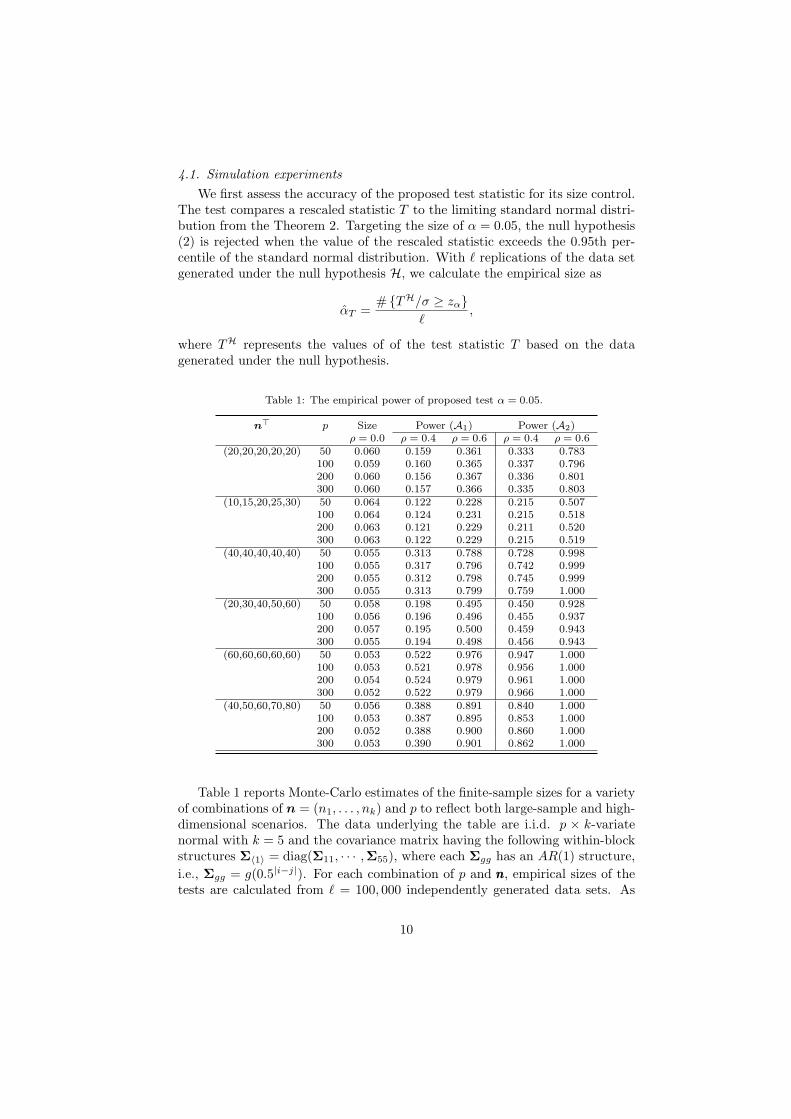
Table 1: The empirical power of proposed test α = 0.05.

n⊤ p Size Power (A1) Power (A2)ρ = 0.0 ρ = 0.4 ρ = 0.6 ρ = 0.4 ρ = 0.6

(20,20,20,20,20) 50 0.060 0.159 0.361 0.333 0.783100 0.059 0.160 0.365 0.337 0.796200 0.060 0.156 0.367 0.336 0.801300 0.060 0.157 0.366 0.335 0.803

(10,15,20,25,30) 50 0.064 0.122 0.228 0.215 0.507100 0.064 0.124 0.231 0.215 0.518200 0.063 0.121 0.229 0.211 0.520300 0.063 0.122 0.229 0.215 0.519

(40,40,40,40,40) 50 0.055 0.313 0.788 0.728 0.998100 0.055 0.317 0.796 0.742 0.999200 0.055 0.312 0.798 0.745 0.999300 0.055 0.313 0.799 0.759 1.000

(20,30,40,50,60) 50 0.058 0.198 0.495 0.450 0.928100 0.056 0.196 0.496 0.455 0.937200 0.057 0.195 0.500 0.459 0.943300 0.055 0.194 0.498 0.456 0.943

(60,60,60,60,60) 50 0.053 0.522 0.976 0.947 1.000100 0.053 0.521 0.978 0.956 1.000200 0.054 0.524 0.979 0.961 1.000300 0.052 0.522 0.979 0.966 1.000

(40,50,60,70,80) 50 0.056 0.388 0.891 0.840 1.000100 0.053 0.387 0.895 0.853 1.000200 0.052 0.388 0.900 0.860 1.000300 0.053 0.390 0.901 0.862 1.000

Table 1 reports Monte-Carlo estimates of the finite-sample sizes for a varietyof combinations of n = (n1, . . . , nk) and p to reflect both large-sample and high-dimensional scenarios. The data underlying the table are i.i.d. p × k-variatenormal with k = 5 and the covariance matrix having the following within-blockstructures Σ⟨1⟩ = diag(Σ11, · · · ,Σ55), where each Σgg has an AR(1) structure,

i.e., Σgg = g(0.5|i−j|). For each combination of p and nnn, empirical sizes of thetests are calculated from ℓ = 100, 000 independently generated data sets. As

10

expected, in general, the tests have their sizes converging to the the nominallevel 0.05 as both p and nk increase together. For certain combinations of p andnk, the test sizes are not very satisfactory when nk are very small, but they allbecome close to the nominal 0.05 level when nk get above 40-50, indicating thatthe asymptotic properties of T described by Theorem 2 pitch in.

Next, we consider the power of the tests, as studied in Section 2. Theempirical power is calculated as

βT =# TA/σ ≥ zα

ℓ,

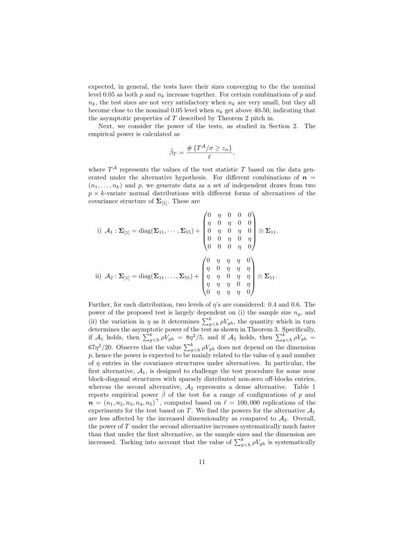
where TA represents the values of the test statistic T based on the data gen-erated under the alternative hypothesis. For different combinations of n =(n1, . . . , nk) and p, we generate data as a set of independent draws from twop × k-variate normal distributions with different forms of alternatives of thecovariance structure of Σ[1]. These are

i) A1 : Σ[1] = diag(Σ11, · · · ,Σ55) +

0 η 0 0 0η 0 η 0 00 η 0 η 00 0 η 0 η0 0 0 η 0

⊗Σ11.

ii) A2 : Σ[1] = diag(Σ11, . . . ,Σ55) +

0 η η η 0η 0 η η ηη η 0 η ηη η η 0 η0 η η η 0

⊗Σ11.

Further, for each distribution, two levels of η’s are considered: 0.4 and 0.6. Thepower of the proposed test is largely dependent on (i) the sample size ng, and

(ii) the variation in η as it determines∑k

g<h ρVgh, the quantity which in turndetermines the asymptotic power of the test as shown in Theorem 3. Specifically,if A1 holds, then

∑kg<h ρVgh = 8η2/5, and if A2 holds, then

∑kg<h ρVgh =

67η2/20. Observe that the value∑k

g<h ρVgh does not depend on the dimensionp, hence the power is expected to be mainly related to the value of η and numberof η entries in the covariance structures under alternatives. In particular, thefirst alternative, A1, is designed to challenge the test procedure for some nearblock-diagonal structures with sparsely distributed non-zero off-blocks entries,whereas the second alternative, A2 represents a dense alternative. Table 1reports empirical power β of the test for a range of configurations of p andn = (n1, n2, n3, n4, n5)

⊤, computed based on ℓ = 100, 000 replications of theexperiments for the test based on T . We find the powers for the alternative A1

are less affected by the increased dimensionality as compared to A2. Overall,the power of T under the second alternative increases systematically much fasterthan that under the first alternative, as the sample sizes and the dimension areincreased. Tacking into account that the value of

∑kg<h ρVgh is systematically

11

larger underA2 as compared toA1, this is a natural trend. And when η increasesfrom 0.4 to 0.6 the power gets larger under both alternatives since the increaseof η contributes to the increase of each ρVgh, which measures the departurefrom the null hypothesis. With η increased under the second alternative, manyentries of empirical powers of the test approach 1, which could be viewed as anempirical indication of the proposed test being consistent.

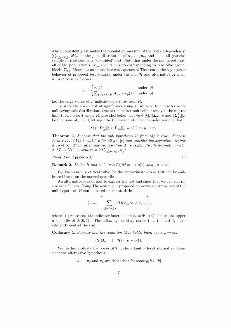
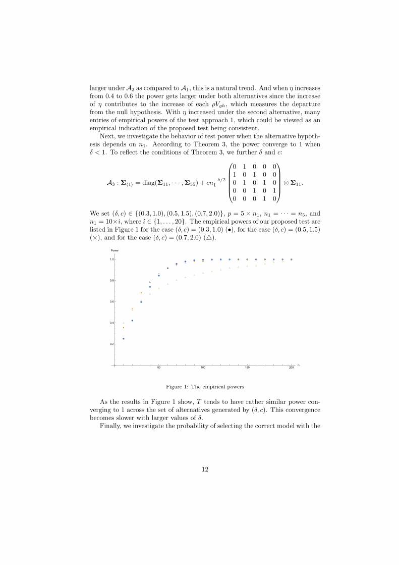
Next, we investigate the behavior of test power when the alternative hypoth-esis depends on n1. According to Theorem 3, the power converge to 1 whenδ < 1. To reflect the conditions of Theorem 3, we further δ and c:

A3 : Σ⟨1⟩ = diag(Σ11, · · · ,Σ55) + cn−δ/21

0 1 0 0 01 0 1 0 00 1 0 1 00 0 1 0 10 0 0 1 0

⊗Σ11.

We set (δ, c) ∈ (0.3, 1.0), (0.5, 1.5), (0.7, 2.0), p = 5 × n1, n1 = · · · = n5, andn1 = 10×i, where i ∈ 1, . . . , 20. The empirical powers of our proposed test arelisted in Figure 1 for the case (δ, c) = (0.3, 1.0) (•), for the case (δ, c) = (0.5, 1.5)(×), and for the case (δ, c) = (0.7, 2.0) ().

×

×

×

×

×

×

×

××

× × × × × × × × × × ×

50 100 150 200n1

0.2

0.4

0.6

0.8

1.0

Power

Figure 1: The empirical powers

As the results in Figure 1 show, T tends to have rather similar power con-verging to 1 across the set of alternatives generated by (δ, c). This convergencebecomes slower with larger values of δ.

Finally, we investigate the probability of selecting the correct model with the

12

proposed multiple comparison procedure. Let Σ⟨1⟩ has the following structure

Σ⟨1⟩ = diag(Σ11, . . . ,Σ44) +

0

√2η 0 0√

2η 0√6η 0

0√6η 0 2

√3η

0 0 2√3η 0

⊗Σ11.

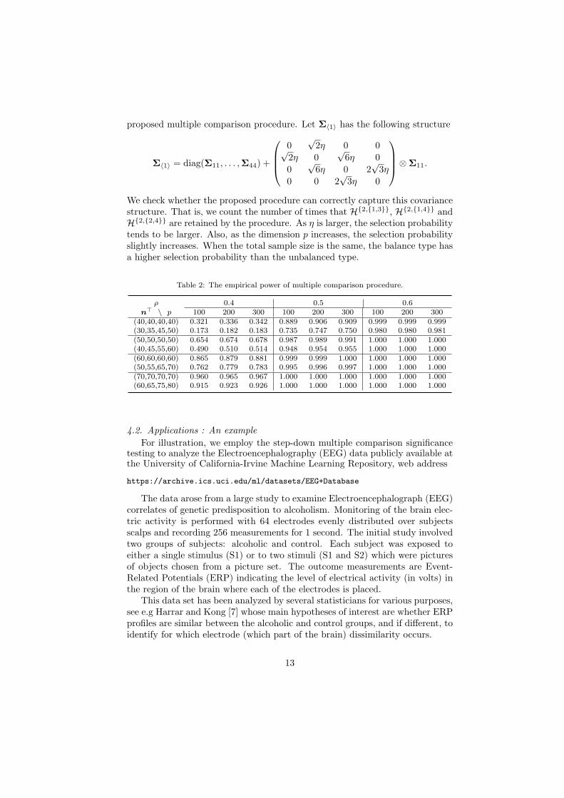
We check whether the proposed procedure can correctly capture this covariancestructure. That is, we count the number of times that H2,1,3, H2,1,4 andH2,2,4 are retained by the procedure. As η is larger, the selection probabilitytends to be larger. Also, as the dimension p increases, the selection probabilityslightly increases. When the total sample size is the same, the balance type hasa higher selection probability than the unbalanced type.

Table 2: The empirical power of multiple comparison procedure.

ρ 0.4 0.5 0.6n⊤ \ p 100 200 300 100 200 300 100 200 300

(40,40,40,40) 0.321 0.336 0.342 0.889 0.906 0.909 0.999 0.999 0.999(30,35,45,50) 0.173 0.182 0.183 0.735 0.747 0.750 0.980 0.980 0.981(50,50,50,50) 0.654 0.674 0.678 0.987 0.989 0.991 1.000 1.000 1.000(40,45,55,60) 0.490 0.510 0.514 0.948 0.954 0.955 1.000 1.000 1.000(60,60,60,60) 0.865 0.879 0.881 0.999 0.999 1.000 1.000 1.000 1.000(50,55,65,70) 0.762 0.779 0.783 0.995 0.996 0.997 1.000 1.000 1.000(70,70,70,70) 0.960 0.965 0.967 1.000 1.000 1.000 1.000 1.000 1.000(60,65,75,80) 0.915 0.923 0.926 1.000 1.000 1.000 1.000 1.000 1.000

4.2. Applications : An example

For illustration, we employ the step-down multiple comparison significancetesting to analyze the Electroencephalography (EEG) data publicly available atthe University of California-Irvine Machine Learning Repository, web address

https://archive.ics.uci.edu/ml/datasets/EEG+Database

The data arose from a large study to examine Electroencephalograph (EEG)correlates of genetic predisposition to alcoholism. Monitoring of the brain elec-tric activity is performed with 64 electrodes evenly distributed over subjectsscalps and recording 256 measurements for 1 second. The initial study involvedtwo groups of subjects: alcoholic and control. Each subject was exposed toeither a single stimulus (S1) or to two stimuli (S1 and S2) which were picturesof objects chosen from a picture set. The outcome measurements are Event-Related Potentials (ERP) indicating the level of electrical activity (in volts) inthe region of the brain where each of the electrodes is placed.

This data set has been analyzed by several statisticians for various purposes,see e.g Harrar and Kong [7] whose main hypotheses of interest are whether ERPprofiles are similar between the alcoholic and control groups, and if different, toidentify for which electrode (which part of the brain) dissimilarity occurs.

13

In this paper, we conduct the analysis the for the single stimulus (S1) expo-sure in the alcoholic group. We are interested in testing the independence of thelevel of electrical activity withing the frontal regions of the brain. Specifically,the data set we focus on, consists of four channels (electrodes) FC1, FCz, FC2and Cz where each channel has names identifying the location of the electrodeon the scalp; F stands for frontal lobe, letter z (zero) is used for the mid-lineand C identifies the central location between the frontal and parietal lobes.Combinations of two letters indicates intermediate locations, for example FC isin between frontal and central electrode locations (see Figure 5 of Harrar andKong [7] for illustration). In the notations of the paper, this data set comprisesk = 4 sub-vectors (FC1 (1), FCz (2), FC2 (3), Cz (4)), each of dimensionalityp = 256 with equal sample sizes, that is ni = 77 for i = 1, . . . , k. The multiplecomparison procedure proposed in Section 3 is applied to clarify whether thelevels of the brain activity at FC1, FCz, FC2 and Cz channels are mutuallyindependent. By setting the significance level as α = 0.05, the testing model isestablished in a stepwise fashion as follows.

Step 1. We test hypothesis H4,1,2,3,4.We calculate test statistic T 4,1,2,3,4/σ4,1,2,3,4 ≈ 32.44, and we alsoobtain z0.05 ≈ 1.645 as an approximate critical value. Therefore, we rejectH4,1,2,3,4 and move on to Step 2.

Step 2. We test following hypotheses:

H3,1,2,3, H3,1,2,4, H3,1,3,4, H3,2,3,4.

The test statistic corresponding to each hypothesis is calculated as follows:

T 3,1,2,3/σ3,1,2,3 ≈ 44.56, T 3,1,2,4/σ3,1,2,4 ≈ 18.43,

T 3,1,3,4/σ3,1,3,4 ≈ 15.94, T 3,2,3,4/σ3,2,3,4 ≈ 12.84.

We also obtain z0.05 ≈ 1.645 as an approximate critical value. Therefore,we reject all hypotheses and move on to Step 3.

Step 3. We test following hypotheses:

H2,1,2, H2,1,3, H2,1,4, H2,2,3, H2,2,4, H2,3,4

The test statistic corresponding to each hypothesis is calculated as follows:

T 2,1,2/σ2,1,2 ≈ 29.41, T 2,1,3/σ2,1,3 ≈ 26.38,

T 2,1,4/σ2,1,4 ≈ 1.45, T 2,2,3/σ2,2,3 ≈ 21.39,

T 2,2,4/σ2,2,4 ≈ 1.06, T 2,3,4/σ2,3,4 ≈ −0.22.

We also obtain z1−√0.95 ≈ 1.955 as an approximate critical value.

To summarize, the hypotheses H2,1,2, H2,1,3, H2,2,3 are rejected,whereas H2,1,4, H2,2,4, H2,3,4 are retained. Hence, with the results

14

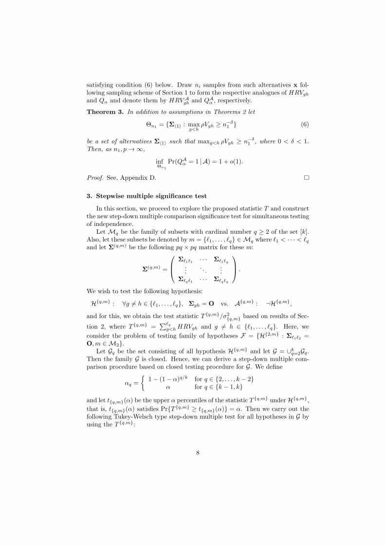
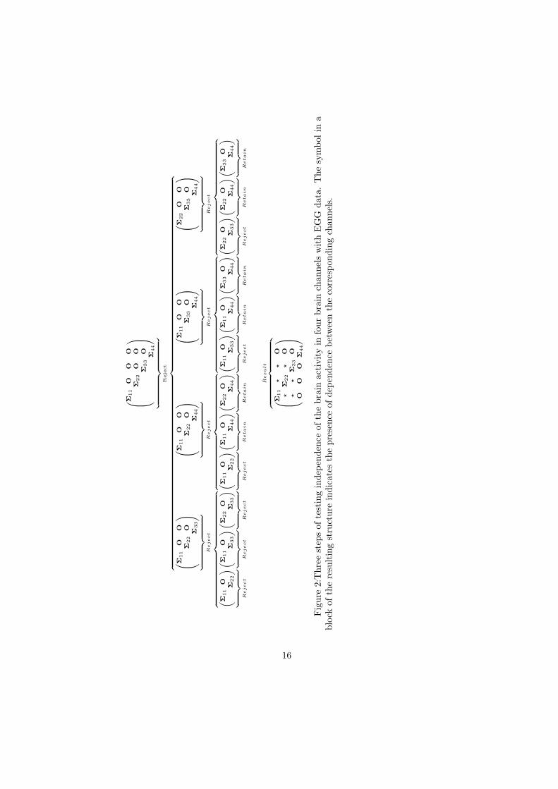
above we have strong evidence to believe that the three channels, FC1, FCz,and FC2 correlate with each other, but there is no correlation between (FC1,FCz, FC2) and Cz. This suggests that the assumption on the cross-channelindependence in such empirical studies may not be appropriate. The four stepsof the testing model for this example are illustrated on the Figure below.

15

Σ11

OO

OΣ

22

OO

Σ33

OΣ

44

︸

︷︷︸

Reje

ct

︷︸︸

︷ Σ

11

OO

Σ22

OΣ

33

︸

︷︷︸

Reject

Σ11

OO

Σ22

OΣ

44

︸

︷︷︸

Reject

Σ11

OO

Σ33

OΣ

44

︸

︷︷︸

Reject

Σ22

OO

Σ33

OΣ

44

︸

︷︷︸

Reject

︷︸︸

︷( Σ

11

OΣ

22

)︸

︷︷︸

Reject

( Σ11

OΣ

33

)︸

︷︷︸

Reject

( Σ22

OΣ

33

)︸

︷︷︸

Reject

︷︸︸

︷( Σ

11

OΣ

22

)︸

︷︷︸

Reject

( Σ11

OΣ

44

)︸

︷︷︸

Retain

( Σ22

OΣ

44

)︸

︷︷︸

Retain

︷︸︸

︷( Σ

11

OΣ

33

)︸

︷︷︸

Reject

( Σ11

OΣ

44

)︸

︷︷︸

Retain

( Σ33

OΣ

44

)︸

︷︷︸

Retain

︷︸︸

︷( Σ

22

OΣ

33

)︸

︷︷︸

Reject

( Σ22

OΣ

44

)︸

︷︷︸

Retain

( Σ33

OΣ

44

)︸

︷︷︸

Retain

Result

︷︸︸

︷ Σ

11

⋆⋆

O⋆

Σ22

⋆O

⋆⋆

Σ33

OO

OO

Σ44

Figure

2:Threestepsof

testingindep

enden

ceof

thebrain

activityin

fourbrain

chan

nelswithEGG

data.Thesymbolin

ablock

oftheresultingstructure

indicatesthepresence

ofdep

enden

cebetweenthecorrespon

dingchan

nels.

16

5. Summary

A test statistic for mutual independence of k random vectors coming for multi-variate normal populations is developed when the dimensionality is large, pos-sibly much larger than the sample size. Such a test is usually carried out as apreliminary test in large scale multivariate inference; examples include discrim-inant analysis or model-based clustering, testing equality of mean vectors andcovariance matrices where the ability to detect departures from independenceis of crucial importance.

With a view towards alternatives in which dependence is spread out overvector components, the test statistic is formed as a sum of consistent estimatorsof the pairwise vector correlation coefficients. The corresponding asymptotictheory is then developed to derive the asymptotic normal limit of the proposedtest when both sample size and dimensionality go to infinity. A step-downmultiple comparison procedure that allows to controls the family-wise errorrate under independence is presented as a direct by-product.

Simulation results are used to demonstrate the finite sample performance ofthe test with respect to its size control and power, for large samples, arbitrarydimensions and a variety of dependence structure models often used in multivari-ate analysis. Our methodology is illustrated with the Electroencephalography(EEG) data where we applied the proposed step-down procedure for assessmentof independence of electrical activity over certain regions of the human brain.

6. Acknowledgements

The research of the first and second authors were supported by JSPS KAK-ENHI Grant Numbers 17K14238, 17K00056. The third author is in part sup-ported by Grant 2013-45266 of the National Research Council of Sweden (VR).

References

[1] T. W. Anderson, An Introduction to Multivariate Statistical Analy-sis,thirded., John Wiley and Sons, NewYork, 2003.

[2] Z. Bai, H. Saranadasa, Effect of high dimension: by an example of twosample problem, Statistica Sinica 6 (1996), 311–329.

[3] Y. Escoufier, Le Traitement des Variables Vectorielles, Biometrics 29 (1973)751–760.

[4] B. Efron, Are a set of microarrays independent of each other?, The Annalsof Applied Statistics 3 (3) (2009), 922–942.

[5] K. T. Fang, Y. T. Zhang, Generalized Multivariate Analysis. Springer,1990.

[6] Han, F. and Liu, H. (2014). Distribution-free tests of independence withapplications to testing more structures. ArXiv:1410.4179.

17

[7] S. W. Harrar, X. Kong, High-dimensional multivariate repeated measuresanalysis with unequal covariance matrices, Journal of Multivariate Analysis145 (2016) 1-21.

[8] M. Hyodo, N. Shutoh, T. Nishiyama, T. Pavlenko, Testing block-diagonalcovariance structure for high-dimensional data, Statistica Neerlandica 69(2015) 460–482.

[9] D. Jiang, Z. Bai, S. Zheng, Testing the independence of sets of large-dimensional variables, Science China Mathematics 56 (2013) 135–147.

[10] J. Josse, J. Pages, F. Husson, Testing the significance of the RV coefficient,Computational Statistics and Data Analysis 53 (2008) 82–91.

[11] D. Leung, M. Drton, Testing independence in high dimensions with sumsof rank correlations https://arxiv.org/abs/1501.01732

[12] K. V. Mardia, J. T. Kent, J. M. Bibby, Multivariate analysis. Probabil-ity and Mathematical Statistics: A Series of Monographs and Textbooks.Academic Press, 1979.

[13] K. Pearson, On the criterion that a given system of deviations from theprobable in the case of a correlated system of variables is such that it canbe reasonably supposed to have arisen from random sampling, PhilosophicalMagazine 50 (1900) 157–175.

[14] A. N. Shiryaev, Probability, 2nd Ed., Springer-Verlag, New-York, 1984.

[15] M. S. Srivastava, N. M. Reid, Testing the structure of the covariance ma-trix with fewer observations than the dimension, Journal of MultivariateAnalysis 112 (2012) 156–171.

[16] G. J. Szkely, M. L. Rizzo, The distance correlation t-test of independencein high dimension, Journal of Multivariate Analysis 112 (2013) 193–213.

[17] S. Taskinen, H. Oja, R. H. Randles, Multivariate nonparametric tests ofindependence, Journal of the American Statistical Association 100 (2005)916–925.

[18] Y. Yang, G. Pan, Independence test for high dimensional data based onregularized canonical correlation coefficients, The Annals of Statistics 43(2015) 467–500.

18

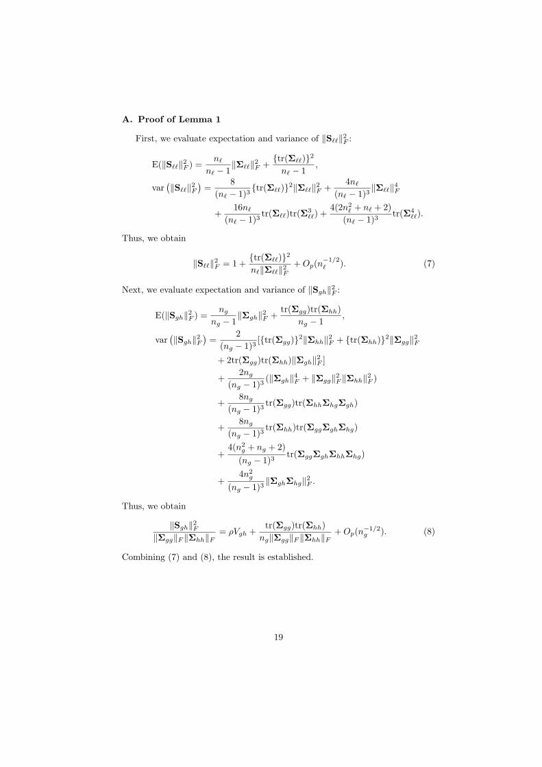
A. Proof of Lemma 1

First, we evaluate expectation and variance of ∥Sℓℓ∥2F :

E(∥Sℓℓ∥2F ) =nℓ

nℓ − 1∥Σℓℓ∥2F +

tr(Σℓℓ)2

nℓ − 1,

var(∥Sℓℓ∥2F

)=

8

(nℓ − 1)3tr(Σℓℓ)2∥Σℓℓ∥2F +

4nℓ

(nℓ − 1)3∥Σℓℓ∥4F

+16nℓ

(nℓ − 1)3tr(Σℓℓ)tr(Σ

3ℓℓ) +

4(2n2ℓ + nℓ + 2)

(nℓ − 1)3tr(Σ4

ℓℓ).

Thus, we obtain

∥Sℓℓ∥2F = 1 +tr(Σℓℓ)2

nℓ∥Σℓℓ∥2F+Op(n

−1/2ℓ ). (7)

Next, we evaluate expectation and variance of ∥Sgh∥2F :

E(∥Sgh∥2F ) =ng

ng − 1∥Σgh∥2F +

tr(Σgg)tr(Σhh)

ng − 1,

var(∥Sgh∥2F

)=

2

(ng − 1)3[tr(Σgg)2∥Σhh∥2F + tr(Σhh)2∥Σgg∥2F

+ 2tr(Σgg)tr(Σhh)∥Σgh∥2F ]

+2ng

(ng − 1)3(∥Σgh∥4F + ∥Σgg∥2F ∥Σhh∥2F )

+8ng

(ng − 1)3tr(Σgg)tr(ΣhhΣhgΣgh)

+8ng

(ng − 1)3tr(Σhh)tr(ΣggΣghΣhg)

+4(n2

g + ng + 2)

(ng − 1)3tr(ΣggΣghΣhhΣhg)

+4n2

g

(ng − 1)3∥ΣghΣhg∥2F .

Thus, we obtain

∥Sgh∥2F∥Σgg∥F ∥Σhh∥F

= ρVgh +tr(Σgg)tr(Σhh)

ng∥Σgg∥F ∥Σhh∥F+Op(n

−1/2g ). (8)

Combining (7) and (8), the result is established.

19

B. Proof of Theorem 1

First, we evaluate the variance of ∥Σgh∥2F , for which we obtain

var(

∥Σgh∥2F)=

2

(ng − 2)(ng + 1)(∥Σgh∥4F + ∥Σgg∥2F ∥Σhh∥2F )

+4(n2

g − 5)

(ng − 2)(ng − 1)(ng + 1)tr(ΣggΣghΣhhΣhg)

+4

ng − 1tr(ΣghΣhg)

2.

From tr(ΣggΣghΣhhΣhg) ≤ ∥Σgg∥F ∥Σhh∥F ∥Σgh∥2F , tr(ΣghΣhg)2 ≤ ∥Σgh∥4F

and ρVgh < 1, we get var( ∥Σgh∥2F )/(∥Σgg∥F ∥Σhh∥F )2 = O(n−1g

). Using

Chebyshev’s inequality, we obtain

∥Σgh∥2F∥Σgg∥F ∥Σhh∥F

= ρVgh + op (1) . (9)

Next, we evaluate the variance of ∥Σℓℓ∥2F for ℓ ∈ g, h. It is obtained by

var(

∥Σℓℓ∥2F)=

4∥Σℓℓ∥4F(nℓ − 2)(nℓ + 1)

+4(2n2

ℓ − nℓ − 7)∥Σ2ℓℓ∥2F

(nℓ − 2)(nℓ − 1)(nℓ + 1).

From ∥Σ2ℓℓ∥2F ≤ ∥Σℓℓ∥4F , we get var( ∥Σℓℓ∥2F )/∥Σℓℓ∥4F = O

(n−1g

). Using Cheby-

shev’s inequality, we obtain

∥Σℓℓ∥2F∥Σℓℓ∥2F

= 1 + op (1) . (10)

From (9) and (10), we obtain HRVgh = ρVgh + op(1).

C. Proof of Theorem 2

From (10), under (A1), ∥Σℓℓ∥F = ∥Σℓℓ∥F (1 + op(1)) for ℓ ∈ g, h. Thus

T = T + op(1), where

T =

k∑g<h

∥Σgh∥2F∥Σgg∥F ∥Σhh∥F

.

Therefore, it sufficient to show the asymptotic normality of T .Under H, we have

∀g ∈ [k], j ∈ [nk] xgj = Σ1/2gg zgj + µg,

20

where zgj ∼ Np(0, Ip) and zgj are mutually independent. We define p × ℓmatrix, Zg(ℓ) = (zg1, . . . , zgℓ) for ℓ ≤ ng. Note that each component of Zg(ng)

independently N (0, 1) distributed. For g < h, i.e. ng ≤ nh, under H,

∥Σgh∥2F =tr(ΣggZg(ng)Z

⊤h(ng)

ΣhhZh(ng)Z⊤g(ng)

)

n2g

−tr(ΣggZg(ng)Z

⊤g(ng)

)tr(ΣhhZh(ng)Z⊤h(ng)

)

n3g

+ op

(∥Σgg∥F ∥Σhh∥F

ng

).

Let Γg be orthogonal matrix s.t. Γ⊤g ΣggΓg = Λg = diag(λg1, . . . , λgp). For

i ∈ [p], we define ugi = (e⊤i Γ⊤g zg1, . . . , e

⊤i Γ

⊤g zgng

)⊤. Then ugi ∼ Nng(0, Ing

)

and e⊤j ugi = z⊤gjΓgei are mutually independent whenever (g, i, j) are distinctindices.

Let ugi(ℓ) = (e⊤i Γ⊤g zg1, . . . , e

⊤i Γ

⊤g zgℓ)

⊤. Then

Γ⊤ggZg(ng) = (ug1(ng), . . . ,ugp(ng))

⊤, Γ⊤hhZh(ng) = (uh1(ng), . . . ,uhp(ng))

⊤.

Using these variables, we rewrite

∥Σgh∥2F = n−2g

p∑i=1

p∑j=1

λgiλhj(u⊤gi(ng)

uhj(ng))2

−n−3g

p∑i=1

p∑j=1

λgiλhju⊤gi(ng)

ugj(ng)u⊤hi(ng)

uhj(ng)

+op

(∥Σgg∥F ∥Σhh∥F

ng

).

Thus T can be expressed as T /σ =∑p

i=1 εi + op(1), where

εi =∑g<h

1

σn2g

[λgiλhi

∥Σgg∥F ∥Σhh∥F

(u⊤

gi(ng)uhi(ng))

2 −∥ugi(ng)∥2∥uhi(ng)∥2

ng

+i−1∑j=0

λgiλhj

∥Σgg∥F ∥Σhh∥F

(u⊤

gi(ng)uhj(ng))

2 −∥ugi(ng)∥2∥uhj(ng)∥2

ng

+

i−1∑j=0

λgjλhi

∥Σgg∥F ∥Σhh∥F

(u⊤

gj(ng)uhi(ng))

2 −∥ugj(ng)∥2∥uhi(ng)∥2

ng

.

Here, for i = 1, both the second and the third term ignore 0. Define F0 = ∅,Ω,and let Fi for i ∈ N be the σ-algebra generated by the random variables Ui−1,where

Ui−1 = (u11, . . . ,u1i−1, . . . ,uk1, . . . ,uki−1).

Then we find that F0 ⊆ · · · ⊆ F∞ and E(εi|Fi−1) = 0. Thus, (εi) is a martingaledifference sequence. We show the asymptotic normality of ε1 + · · · + εp by

21

adapting the martingale difference central limit theorem; see, e.g., [14]. LetEi−1 = E(ε2i |Fi−1). Then

E

(p∑

i=1

Ei−1

)= 1 + o(1), var

(p∑

i=1

Ei−1

)= O(n−1

1 ).

Thus, (I) :∑p

i=1 Ei−1 = 1 + op(1) as n1 → ∞. Also

p∑i=1

E(ε4i ) = O

(k∑

g=1

∥Σ2gg∥2

∥Σgg∥4

).

Thus, under (A1), (II) :∑p

i=1 E(ε4i ) = o(1) as p → ∞. The above results (I)

and (II) complete the proof.

D. Proof of Theorem 3

From (10), the power of our proposed test at Σ⟨1⟩ is Pr(QAα = 1 | A) =

Pr(T ≥ σzα) + o(1) as n1 → ∞. Thus it is sufficient to show that Pr(T ≥σzα) = 1 + o(1) for any Σ⟨1⟩ ∈ Θn1 .

We note that E(T ) =∑

g<h ρVgh > 0 for any Σ⟨1⟩ ∈ Θn1 , and

Pr(T ≥ σzα

)≥ 1− Pr

(|T − E(T )− σzα| ≥ E(T )

).

Using Markov’s inequality and Cauchy-Schwarz inequality in the context ofexpectation, we obtain

Pr(∣∣∣T − E(T )− σzα

∣∣∣ ≥ E(T ))

≤ E(∣∣∣T − E(T )− σzα

∣∣∣ /E(T ))≤ E

(∣∣∣T − E(T )− σzα

∣∣∣2) /E(T )2.

Since E(|T − E(T )− σzα|2) = var(T ) + σ2z2α, we obtain

Pr(T ≥ σzα) ≥ 1− var(T ) + σ2z2α

E(T )2. (11)

We further evaluate var(T ). For any g < h, g, h ∈ [k], we define Agh =

HRV gh − ρVgh, where HRV gh = ∥Σgh∥2F /(∥Σgg∥F ∥Σhh∥F ). Then

var(T )

E(T )2=

E(∑

g<h Agh)2

E(T )2≤

k(k − 1)∑

g<h E(A2gh)

2E(T )2.

22

E(A2gh) is obtained by

E(A2gh) =

2

(ng − 2)(ng + 1)(ρV 2

gh + 1)

+4(n2

g − 5)tr(ΣggΣghΣhhΣhg)

(ng − 2)(ng − 1)(ng + 1)∥Σgg∥2F ∥Σhh∥2F

+4tr(ΣghΣhg)

2(ng − 1)∥Σgg∥2F ∥Σhh∥2F

.

From tr(ΣggΣghΣhhΣhg) ≤ ∥Σgg∥F ∥Σhh∥F ∥Σgh∥2F and tr(ΣghΣhg)2 ≤ ∥Σgh∥4F ,

we getE(A2

gh)

E(T )2= O

(ρVgh + ρV 2

gh

(∑

g<h ρVgh)2ng+

ρV 2gh + 1

(∑

g<h ρVgh)2n2g

)Note that E(T ) =

∑g<h ρVgh ≥ maxg<h ρVgh ≥ n−δ

1 . Thus, for anyΣ⟨1⟩ ∈ Θn1 ,

E(A2gh)

E(T )2= O

(1

n1−δ1

+1

n1+

1

n21

).

Since k is fixed, we obtain

var(T )

E(T )2= O

(1

n1−δ1

+1

n1+

1

n21

). (12)

Next, we evaluate σ2/E(T )2. Since σ2 = O(n−21 ) and E(T )2 ≥ (maxg<h ρVgh)

2 ≥n−2δ1 , we obtain

σ2z2α

E(T )2= O

(1

n2(1−δ)

). (13)

Substituting (12) and (13) to (11), for any Σ⟨1⟩ ∈ Θn1 ,

Pr(T ≥ σzα) = 1 +O

(1

n1−δ1

+1

n2(1−δ)1

+1

n1+

1

n21

).

Therefore, under n1 → ∞, infΘn1Pr(T ≥ σzα) = 1 + o(1).

23