No. 13-3 The 2010 Survey of Consumer Payment Choice:

Technical Appendix

Marco Angrisani, Kevin Foster, and Marcin HitczenkoAbstract: This document serves as the technical appendix to the 2010 Survey of Consumer Payment Choice. The Survey of Consumer Payment Choice (SCPC) is an annual study designed primarily to study the evolving attitudes to and use of various payment instruments by consumers over the age of 18 in the United States. The main report, which introduces the survey and discusses the principal economic results, can be found on http://www.bostonfed.org/economic/cprc/SCPC. In this data report, we detail the technical aspects of the survey design, implementation, and analysis.

JEL codes: D12, D14, E4 Marco Angrisani is an associate economist at the University of Southern California Dornsife Center for Economic and Social Research. Kevin Foster is a survey methodologist and Marcin Hitczenko is a statistician; both are members of the Consumer Payments Research Center in the research department of the Federal Reserve Bank of Boston. Their e-mail addresses are marco.angrisani@usc.edu, kevin.foster@bos.frb.org, and marcin.hitczenko@bos.frb.org, respectively. This paper, which may be revised, is available on the web site of the Federal Reserve Bank of Boston at http://www.bostonfed.org/economic/wp/index.htm. The views expressed in this paper are those of the authors and do not necessarily represent the views of the Federal Reserve Bank of Boston or the Federal Reserve System.

The Survey of Consumer Payment Choice is a product of the Consumer Payments Research Center (CPRC) in the research department at the Federal Reserve Bank of Boston. Staff at the USC Dornsife Center for Economic and Social Research (CESR) and the RAND Corporation also contributed to the production of the survey.

The authors thank their colleagues and management in the CPRC and the Boston Fed research department. In addition, we thank the management and staff at CESR and the RAND Corporation. From the Boston Fed: Tamas Briglevics, Sean Connolly, Kevin Foster, Claire Greene, Marcin Hitczenko, Vikram Jambulapati, Suzanne Lorant, William Murdock, Scott Schuh, Oz Shy, Joanna Stavins, and Bob Triest. From CESR and the RAND Corporation: Tania Gursche, Arie Kapteyn, Bart Orriens, and Bas Weerman. Special thanks go to Erik Meijer from CESR, who contributed to earlier SCPC appendices, which formed the basis for this paper. Finally, the authors acknowledge John Sabelhaus and the staff of the Survey of Consumer Finances at the Federal Reserve Board of Governors for their advice and mentorship. Geoff Gerdes and May Liu from the Board also shared advice and knowledge.

This version: November 18, 2013

Contents

1 Introduction 3

2 Survey Objective, Goals, and Approach 3

2.1 Survey Objective and Goals . . . . . . . . . . . . . . . . . . . . . . . . . . . 4

2.2 Unit of Observation . . . . . . . . . . . . . . . . . . . . . . . . . . . . . . . . 4

2.3 Interview Mode . . . . . . . . . . . . . . . . . . . . . . . . . . . . . . . . . . 5

2.4 Public Use Datasets . . . . . . . . . . . . . . . . . . . . . . . . . . . . . . . 6

3 Questionnaire Changes 6

3.1 Bank and Payment Accounts . . . . . . . . . . . . . . . . . . . . . . . . . . . 7

3.2 Payment Instruments . . . . . . . . . . . . . . . . . . . . . . . . . . . . . . . 7

3.3 Mobile Banking and Mobile Payments . . . . . . . . . . . . . . . . . . . . . 8

3.4 Characteristics of Payment Instruments . . . . . . . . . . . . . . . . . . . . . 8

3.5 Survey Instructions . . . . . . . . . . . . . . . . . . . . . . . . . . . . . . . . 9

3.6 Detailed List of Questionnaire Changes . . . . . . . . . . . . . . . . . . . . . 10

4 Data Collection 10

4.1 American Life Panel . . . . . . . . . . . . . . . . . . . . . . . . . . . . . . . 11

4.2 SCPC Sample Selection . . . . . . . . . . . . . . . . . . . . . . . . . . . . . 14

4.3 Survey Completion . . . . . . . . . . . . . . . . . . . . . . . . . . . . . . . . 16

4.4 Item Response . . . . . . . . . . . . . . . . . . . . . . . . . . . . . . . . . . . 19

5 Sampling Weights 21

5.1 Post-Stratification . . . . . . . . . . . . . . . . . . . . . . . . . . . . . . . . . 21

5.2 Raking Algorithm . . . . . . . . . . . . . . . . . . . . . . . . . . . . . . . . . 21

6 Data Preprocessing 25

6.1 Categorical Data . . . . . . . . . . . . . . . . . . . . . . . . . . . . . . . . . 25

6.2 Quantitative Data . . . . . . . . . . . . . . . . . . . . . . . . . . . . . . . . . 26

6.2.1 Preprocessing: Typical Monthly Payment Use . . . . . . . . . . . . . 28

6.2.2 Preprocessing: Cash Withdrawal . . . . . . . . . . . . . . . . . . . . 32

7 Population Parameter Estimation 36

7.1 Standard Errors and Covariances . . . . . . . . . . . . . . . . . . . . . . . . 38

7.2 Functions of Population Means . . . . . . . . . . . . . . . . . . . . . . . . . 39

7.2.1 Generating U.S. Aggregate Estimates . . . . . . . . . . . . . . . . . . 40

1

8 Hypothesis Tests for Temporal Changes in Consumer Payments 41

8.1 Hypothesis Tests for Means . . . . . . . . . . . . . . . . . . . . . . . . . . . 41

8.1.1 Analysis of Levels: Number of Payments by Payment Method . . . . 42

8.1.2 Analysis of Levels: Number of Payments by Transaction Type . . . . 43

8.1.3 Analysis of Proportions: Adoption Rates . . . . . . . . . . . . . . . . 43

8.2 Hypothesis Tests for Growth Rates . . . . . . . . . . . . . . . . . . . . . . . 44

8.2.1 Analysis of Growth Rates: Number of Payments by Payment Method 45

8.2.2 Analysis of Growth Rates: Number of Payments by Transaction Type 46

8.3 Hypothesis Tests for Shares . . . . . . . . . . . . . . . . . . . . . . . . . . . 46

8.3.1 Analysis of Shares: Number of Payments by Payment Method . . . . 49

8.3.2 Analysis of Shares: Number of Payments by Transaction Type . . . . 51

9 Future Work 51

2

1 Introduction

The Survey of Consumer Payment choice has been conducted annually since 2008 through

a partnership between the Consumer Payment Research Center (CPRC) at the Federal Re-

serve Bank of Boston and the RAND Corporation (from 2013 the partnership will include

the Dornsife Center for Social and Economic Research at the University of Southern Cali-

fornia). Each year, this partnership involves the careful planning and execution of a series

of steps ranging from the gathering to the analysis of the survey data. This begins with

data collection, namely the design of a questionnaire, the selection of the sample, and the

administration of the questionnaire. Once the data are collected, a coherent methodology

for analysis must be adopted. In the case of the SCPC, this involves calculating post-

stratification weights, devising a strategy to clean the data, and developing a model that

allows for population-based inference. In this appendix, we provide details relating to each

of these steps.

The organization of this work is designed to follow the natural, chronological progression of

considerations involved in conducting and analyzing a survey. After establishing the con-

text and goals of the survey in Section 2, we highlight changes in the survey from the 2009

version to the 2010 version. Section 3 discusses the design of the questionnaire, focusing on

the changes from previous years’ versions. In Section 4 we begin by detailing the selection

and composition of the survey sample and present statistics related to survey response and

completion. Section 5 delineates the generation and properties of the sample weights devel-

oped to make inferences about the entire population of U.S. consumers. Section 6 discusses

our general philosophy towards data preprocessing of categorical and quantitative variables,

and provides details of two new data-editing procedures. In Section 7, we give details about

the assumed mathematical models used to determine the population estimates and their

standard errors. Section 8 builds on these results by conducting a variety of hypothesis

tests. The hypothesis tests are mostly applied to the SCPC data concerning the number

of payments, by instrument and transaction type. Finally, Section 9 describes work that is

being done by the CPRC and RAND to improve the survey and its analysis.

2 Survey Objective, Goals, and Approach

In this section we describe the SCPC survey program’s overall objectives, goals, and ap-

proach, and explain the choices made in choosing the observation unit and the interview

mode of the SCPC. In both cases, the choices were made to use best survey practices, within

3

the constraints of the SCPC budget.

2.1 Survey Objective and Goals

As noted in Foster, Schuh, and Zhang (2012b), the main objective of the SCPC program

is to measure U.S. consumer payments behavior. The main goals of the program are to

provide aggregate data on trends in U.S. consumer payments and to provide a consumer-

level database to support research on consumer payments.

2.2 Unit of Observation

The SCPC uses the individual consumer as both the sampling unit and the observation

unit. This choice stands in contrast to those of the Survey of Consumer Finances, which

is organized by primary economic units in the household, and the Consumer Expenditure

Survey, which uses the household as the sampling unit and observation unit. The reason the

SCPC uses the individual consumer is that asking one consumer to estimate the payment

behavior and cash behavior of all members of the household would be too burdensome. Each

consumer surveyed is expected to recall only his or her own payments, not those of other

members of his or her household. In addition, asking one individual about all household

members would increase the cost of the incentive payments the survey pays out. SCPC

incentives are based on the average length of time it takes respondents to complete the

survey. Instead of interviewing one consumer about his or her self plus several household

members, we can interview several different consumers and potentially increase the number

of demographic groups included in the sample.

We believe that the consumer surveyed will be able to report accurate accounts of his or her

own payment behavior, but might not be able to accurately estimate the payment behavior of

other household members. This is especially true for two major sections of the survey. In the

Cash Use section, we ask consumers to recall where they get cash, how much cash they get,

and how often they get it. In addition, we ask the consumers to report the amount of cash on

their person—in other words, the amount of cash currently in their pocket, wallet, or purse.

Cash differs from other payment instruments in that there is no concept of “joint” ownership

of cash. Each member of a household has his or her own cash, even if it all comes from the

same bank account. Therefore, it is most appropriate to ask the individual consumer about

his or her own cash behavior and not about the cash habits of other household members.

4

The second area of the survey that benefits from using the respondent as the observation

unit is the Payment Use section, where we ask the consumer to estimate the number of

payments he or she makes in a typical period (week, month, or year) (Angrisani, Kapteyn,

and Schuh 2013; Hitczenko 2013b). Only the respondent can accurately estimate the number

of payments he or she makes in a typical time period. It would be impossible for the average

consumer to know the complete payment behavior of all members of the household. We

believe this gives us more accurate measurements of the number of nonbill payments made

by consumers. In addition, we ask respondents to tell us their level of responsibility for

several household tasks, such as shopping or paying bills. This allows us to compare the

number of payments reported by the respondent with those reported by others with similar

levels of responsibility.

However, we believe that interviewing the consumer as the unit of observation may lead to

some double counting in the bills section of Payment Use, due to the fact that bills are often

a household expense, rather than a personal one. To accurately measure bills, it might be

better to ask about the entire household’s bill payment behavior. Currently, the SCPC asks

respondents to estimate only the number of bills that they physically pay themselves, either

by mail, by phone, online, or in person. Ongoing research will allow us to determine better

ways to ask about household bills.

2.3 Interview Mode

The SCPC is a computer-assisted web interview (CAWI). This mode of interview fits best

with our sampling frame, which is the internet-based American Life Panel (ALP), jointly

run by RAND and the Center for Social and Economic Research at USC.1 To minimize

undercoverage, all ALP members are given internet access upon recruitment into the panel.

The survey instrument is the MMIC survey system, developed by the RAND Corporation.2

The CAWI mode is beneficial to the SCPC because of the length of the survey. The median

duration for taking each year of the survey is around 30 minutes. Using a CAWI allows

the respondent to log off and come back to the survey later if interrupted. In addition, it

is cheaper than using face-to-face interviews or telephone because no interviewers need to

be paid. Finally, respondents may be more willing to answer some sensitive questions, like

the amount of cash stored in their home, if the survey is conducted via the web (De Leeuw

2005).

1More information about the ALP can be found at https://mmicdata.rand.org/alp/.2More information on MMIC is available at https://mmicdata.rand.org/mmic/index.php.

5

2.4 Public Use Datasets

The 2010 SCPC data can be downloaded from the Boston Fed’s SCPC website.3 The data

are available in Stata, SAS, and CSV formats. Before starting any analysis, it is highly

recommended that the data user read the companion document, “2010 SCPC Data User’s

Guide” (Foster 2013), which is available at the same website. In addition, it is useful to read

the warning against using consumer-level estimates to aggregate up to U.S. total population

estimates, in Section 7.2.1 of this paper.

Users who are interested in downloading the original, raw datasets can obtain these from the

RAND Corporation’s website. The Boston Fed SCPC website contains a link to the RAND

data download site. Interested users must create a username and password to download data

from the RAND website. These data contain only the survey variables. These data have

not been cleaned for outliers and there are no created variables in the dataset. Additionally,

survey items that allow the respondent to choose a frequency have not been converted to

a common frequency, and randomized variables have not been unrandomized. The variable

prim key is the primary key for both the RAND and the Boston Fed datasets, and this

variable can be used to merge the raw, uncleaned data from RAND with the Boston Fed’s

processed dataset.

3 Questionnaire Changes

The SCPC questionnaire is written by the CPRC and is available for viewing at http:

//www.bostonfed.org/economic/cprc/SCPC. For the most part, the survey questions for

2010 are the same or similar to the previous year’s version, although there are changes

introduced every year either to collect new information or to collect the same information

in a better way. Between 2009 and 2010, the CPRC made relatively fewer changes to

the survey questionnaire than in previous years. This section describes the changes to the

economic definitions and scope, which improved and clarified the measurement of many

consumer payment choices, and the changes to the questionnaire design and methodology,

which improved the measurement of consumer payment concepts. The section also includes

a detailed listing of all changes in questionnaire content.

3http://www.bostonfed.org/economic/cprc/SCPC

6

3.1 Bank and Payment Accounts

The basic categories and definitions of accounts that fund consumer payments as presented

in the 2009 SCPC were mostly preserved, while changes were made in the 2010 SCPC to

improve respondents’ understanding of the concept of money market accounts. Specifically,

the 2010 SCPC questionnaire displayed the definition for money market accounts on the

screen with the question asking the respondent about the number of money market accounts

held. In the 2009 SCPC, the respondent had to click on the word “money market account”

to see the definition. The SCPC definitions of both money market accounts and savings

accounts are derived from the definitions in the Federal Reserve Board’s Survey of Consumer

Finances.

3.2 Payment Instruments

Because the SCPC measures the adoption and use of payment instruments by consumers,

the payment instrument is a central concept in the survey. While the 2010 SCPC inherited

the set of payment instruments covered from the 2009 SCPC and preserved the structure and

organization of the questionnaire, it also introduced new questions and enhanced definitions

and instructions in order to achieve a more comprehensive and accurate measurement of con-

sumers’ payment behavior with payment instruments. The 2010 SCPC made the following

specific improvements to better measure adoption of payment instruments:

• Check – Respondents were asked whether they had written a paper check to make a

payment in the past 12 months. The responses to this question enhance the definition

of check adoption to make it consistent with the definition of other paper instruments,

which is that the consumer either currently has on hand, or has used the instrument

in a particular period or a typical period.

• Credit card – The category “Branded cards,” as it appeared in the 2009 SCPC, was

rephrased to be “Store branded cards.” This change was intended to improve respon-

dent recall and understanding, and thus to yield a better measure of the adoption of

different types of credit cards.

• Prepaid card – The category “Specific purpose,” as it appeared in the 2009 SCPC,

was rephrased to be “Merchant specific.” The new category “Government issued” was

introduced in the 2010 SCPC to replace the category “Electronic Benefits Transfer

(EBT),” as it appeared in the 2009 SCPC. The notion of “Government issued” is a

7

much broader concept that covers not only EBT cards, but also other government ben-

efits cards such as Direct Express. These changes are intended to improve respondent

recall and understanding, and thus to yield a better measure of prepaid card adoption.

The 2010 SCPC also began to measure the dollar value stored on prepaid cards that

respondents currently hold. In addition, the question that probes how consumers reload

their prepaid cards added two options, “Rewards from loyalty program” and “Refund

or store credit,” to the existing list of possible venues of reloading.

In the wake of the Durbin Amendment to the Dodd-Frank Act, two new questions were

added to understand consumer preferences for debit card transactions.

• Debit card authorization – Starting in the 2010 SCPC, respondents were asked in which

way they prefer to complete a debit card transaction. The choices included: “PIN,”

“Signature,” “Indifferent,” and “Neither one.”

• Debit card security – This question is fully described in Section 3.4.

3.3 Mobile Banking and Mobile Payments

To capture the recent innovations and emerging developments in mobile banking and mobile

payments in the United States, the 2010 SCPC improved its measurement of these activities.

• Cell phone – Respondents were asked about the following features of their mobile

phone: Using text/SMS with no texting plan; Using text/SMS with texting plan; Web

browsing; Smart phone such as iPhone, Android, or BlackBerry.

• Mobile banking – Respondents were asked whether they have set up mobile banking

and if so, whether they have used it in the past 12 months.

• Mobile payments – The list of available response options to conduct a mobile payment

was expanded in 2010 to cover payments made by using a mobile phone to scan a

barcode.

3.4 Characteristics of Payment Instruments

The 2010 SCPC expanded the section of the assessment of characteristics of payment in-

struments and added new questions to assess payments made in different locations. An

8

additional question was added to further understand consumers’ preference for authorizing

debit card payments.

• Characteristics of payment instruments – While retaining the four characteristics as-

sessed by consumers in the 2009 SCPC, namely, “Security,” “Acceptance of Payment,”

“Cost,” and “Convenience,” the 2010 SCPC reinstated two other characteristics that

were assessed in the 2008 SCPC but dropped in the 2009 SCPC. The two characteris-

tics are “Getting & Setting Up” and “Payment Records.” As a result, the 2010 SCPC

asked consumers to rank six characteristics when they decide which payment method

to use, as opposed to four in the 2009 SCPC.

• Security of payment locations – Starting from the 2010 SCPC, consumers were asked

to assess the security feature of different payment locations. The five locations assessed

by the 2010 SCPC are: in person, online, by mail, by phone, and via mobile payments.

• Security of debit cards – In response to the Durbin Amendment to the Dodd-Frank

Act, the 2010 SCPC added a separate question to probe consumers’ assessment of the

security of different ways of using a debit card. Specifically, four ways of authoriz-

ing a debit card transaction were listed for assessment: PIN authorization, signature

authorization, no PIN and no signature authorization, and using a debit card online.

3.5 Survey Instructions

A final change was to improve some of the instructions that appear on the screen as the

respondent completes the online questionnaire. Many of these improvements are in the

Frequency of Use section of the survey, which produces estimates of the number of payments

made in a typical month.

To reduce the frequency of responses of improbably large numbers of payments per period

(week, month, or year), the 2010 SCPC introduced several new instructions. The respondent

was asked to answer only for his or her self, and not for the household. The instructions

also remind the respondent that we are asking for number of payments, not the dollar value

of payments. In addition, the survey clarifies the definition of automatic bill payments and

how they differ from online bill payments.

Finally, the 2010 SCPC introduced better automated error checking to the online survey

instrument. These error checks take the form of better skip patterns, which prevent re-

spondents from seeing questions that are not consistent with their previous responses, and

9

improved error messages, which point the respondent to exactly what might be wrong. Fol-

lowing good survey practice, the survey instrument gives respondents the opportunity to

change their answers if we believe them to be wrong (for example, reporting that they write

100 checks per week), but it never forces a respondent to change an answer.

3.6 Detailed List of Questionnaire Changes

The 2010 questionnaire changes described in the preceding sections of this appendix were

introduced primarily in three ways:

1. 2009 questions were deleted, Table 1

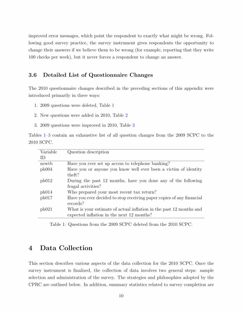
2. New questions were added in 2010, Table 2

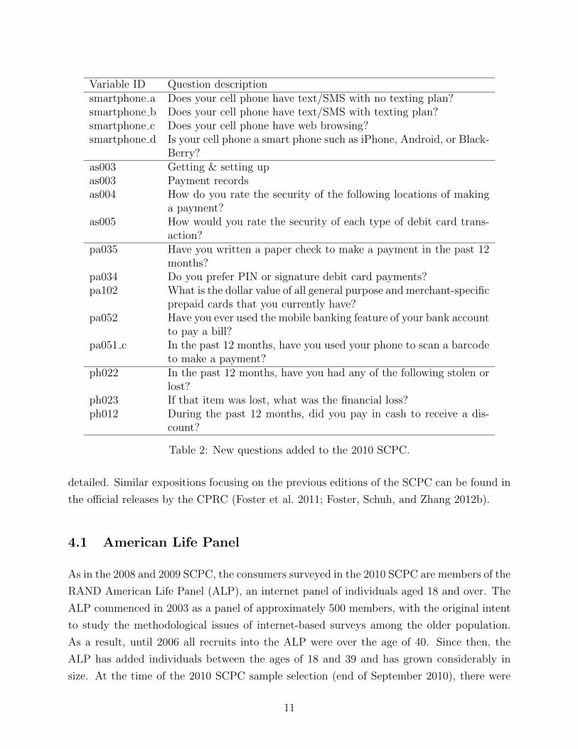
3. 2009 questions were improved in 2010, Table 3

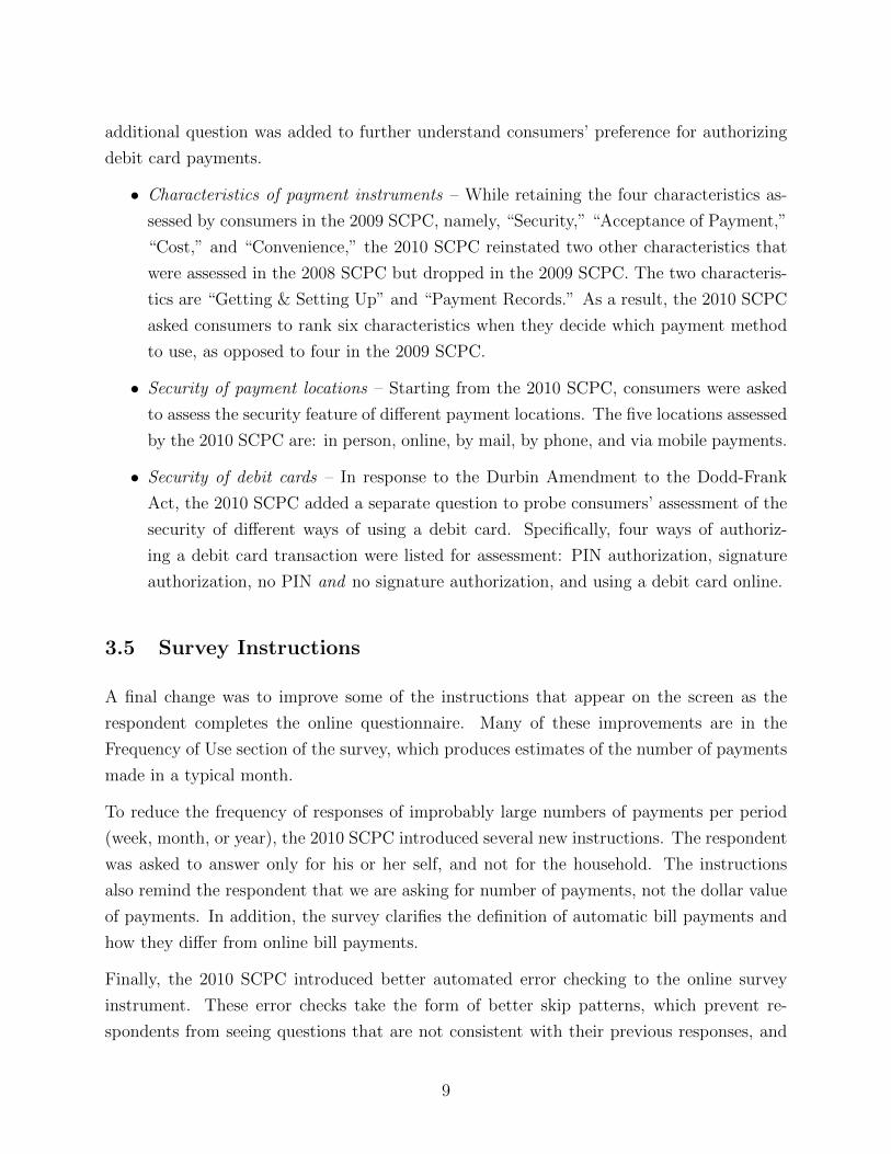
Tables 1–3 contain an exhaustive list of all question changes from the 2009 SCPC to the

2010 SCPC.

VariableID

Question description

newtb Have you ever set up access to telephone banking?ph004 Have you or anyone you know well ever been a victim of identity

theft?ph012 During the past 12 months, have you done any of the following

frugal activities?ph014 Who prepared your most recent tax return?ph017 Have you ever decided to stop receiving paper copies of any financial

records?ph021 What is your estimate of actual inflation in the past 12 months and

expected inflation in the next 12 months?

Table 1: Questions from the 2009 SCPC deleted from the 2010 SCPC.

4 Data Collection

This section describes various aspects of the data collection for the 2010 SCPC. Once the

survey instrument is finalized, the collection of data involves two general steps: sample

selection and administration of the survey. The strategies and philosophies adopted by the

CPRC are outlined below. In addition, summary statistics related to survey completion are

10

Variable ID Question descriptionsmartphone a Does your cell phone have text/SMS with no texting plan?smartphone b Does your cell phone have text/SMS with texting plan?smartphone c Does your cell phone have web browsing?smartphone d Is your cell phone a smart phone such as iPhone, Android, or Black-

Berry?as003 Getting & setting upas003 Payment recordsas004 How do you rate the security of the following locations of making

a payment?as005 How would you rate the security of each type of debit card trans-

action?pa035 Have you written a paper check to make a payment in the past 12

months?pa034 Do you prefer PIN or signature debit card payments?pa102 What is the dollar value of all general purpose and merchant-specific

prepaid cards that you currently have?pa052 Have you ever used the mobile banking feature of your bank account

to pay a bill?pa051 c In the past 12 months, have you used your phone to scan a barcode

to make a payment?ph022 In the past 12 months, have you had any of the following stolen or

lost?ph023 If that item was lost, what was the financial loss?ph012 During the past 12 months, did you pay in cash to receive a dis-

count?

Table 2: New questions added to the 2010 SCPC.

detailed. Similar expositions focusing on the previous editions of the SCPC can be found in

the official releases by the CPRC (Foster et al. 2011; Foster, Schuh, and Zhang 2012b).

4.1 American Life Panel

As in the 2008 and 2009 SCPC, the consumers surveyed in the 2010 SCPC are members of the

RAND American Life Panel (ALP), an internet panel of individuals aged 18 and over. The

ALP commenced in 2003 as a panel of approximately 500 members, with the original intent

to study the methodological issues of internet-based surveys among the older population.

As a result, until 2006 all recruits into the ALP were over the age of 40. Since then, the

ALP has added individuals between the ages of 18 and 39 and has grown considerably in

size. At the time of the 2010 SCPC sample selection (end of September 2010), there were

11

VariableID

Question description Description of change

as012 Rank the importance of each pay-ment characteristic when you de-cide what payment instrument touse.

Added rows for Getting & settingup and Payment records

pa019 c Do you have any of the followingtypes of credit cards?

Changed terminology from“Branded” to “Store branded”

pa054 c Tell us the numbers of creditcards of each type (both rewardsand non-rewards cards)

Changed terminology from“Branded” to “Store branded”

pa099 b Do you have any of the followingtypes of prepaid cards?

Changed terminology from “Spe-cific purpose” to “Merchant spe-cific”

pa100 b How many of each type of prepaidcard do you have?

Changed terminology from “Spe-cific purpose” to “Merchant spe-cific”

pa099 d Do you have any of the followingtypes of prepaid cards?

Changed terminology from “Elec-tronic benefits transfer” to “Gov-ernment issued”

pa100 d How many of each type of prepaidcard do you have?

Changed terminology from “Elec-tronic benefits transfer” to “Gov-ernment issued”

pa101 For prepaid card reloaders only:Thinking about the prepaid cardthat you reload most often, whatis the most common way that youreload that card?

Added “Rewards from loyaltyprogram” and “Refund or storecredit” as response options.

Table 3: Questions changed from the 2009 to 2010 SCPC.

3,260 panelists. There are several pathways that lead individuals into the ALP, but from

a survey methodological point of view these group into two recruiting strategies. The first

strategy involves gathering volunteers from other, already-established panels. The second

strategy involves asking individuals already in the ALP to recommend acquaintances to be

potential members. Members recruited in the latter manner remain linked to an external

panel through the original recruit. Overall, while new sources of members have been added

since September 2010, at that time there were five cohorts in the ALP. They are described

briefly below.4

4The reference names and acronyms for the ALP cohorts are different from those used in the previousreports. Reference names and acronyms adopted here are more in line with those used to describe sourcesand type of recruitment in the dataset.

12

1. Monthly Survey (MS) cohort

Individuals recruited from those who had answered the Monthly Survey (MS) of the

University of Michigan’s Survey Research Center.

2. National Survey Project (NSP) cohort: http://www.sca.isr.umich.edu/

Individuals recruited from those who had participated in the Face-to-Face Recruited

Internet Survey Platform at Stanford University and Abt SRBI. This panel was ter-

minated in September 2009.

3. Survey Sampling International (SSI) cohort: http://www.surveysampling.com

Individuals recruited via postal mail and phone through Survey Sampling International

as part of an experiment to test different recruitment methods.

4. American Life Panel Household (ALPH) cohort:

Individuals living in the same household as already-existing members of the ALP. Each

member is allowed to invite up to three adult individuals from the same household to

join the panel. At the time when the 2010 SCPC was administered, about 12 percent

of sampled households had more than one panel member.

5. Snowball cohort

Individuals first suggested by early ALP members and subsequently contacted by

RAND and asked to join the panel. No new Snowball respondents were recruited

after May 2009, and this cohort is used primarily for survey pretests and experiments.

Indeed, no members of the Snowball cohort feature in the 2009 or 2010 SCPC sample.

It should be noted that ALP members remain in the panel, unless they formally ask to be

removed or stop participating in surveys over a prolonged period of time. At the beginning

of each year, RAND contacts all members who did not take any survey for at least a year

and removes them from the panel, unless they explicitly declare continued interest in par-

ticipating. Since inactive members are removed only once a year, the pool of those invited

to answer the survey at a given point in time may include inactive members.

In its early stages, the ALP was, understandably, not demographically representative of

the U.S. population of adults. First, due to its early research intentions, the panel prior

to 2006 was composed exclusively of individuals above the age of 40. In addition, as the

panel was expanded, members recruited directly from the three already-existing panels(1−3)

were recruited on a volunteer basis, with recruitment rates ranging from around 30 percent

from the MS panel to approximately 50 percent in the NSP panel. Finally, expanding the

13

panel by inviting household members likely skewed the demographic composition further.

Nevertheless, as the ALP has been growing in size, its overall representativeness with respect

to a variety of demographic variables has been improving. Most importantly, there is enough

diversity within the ALP to allow for the creation of stratum weights that match benchmark

numbers in the Current Population Study (CPS). More information about the American Life

Panel can be found at the website http://mmic.rand.org/alp.

4.2 SCPC Sample Selection

The SCPC was originally conceived as a longitudinal panel. The benefits of a longitudinal

panel, namely the added power associated with tracking trends at the individual level, have

been well discussed (Baltagi 2008; Duncan and Kalton 1987; Frees 2004; Lynn 2009). Thus,

for many research agendas, it is advantageous to base results on a longitudinal panel, rather

than on a sequence of cross-sectional studies. As a result, one of the primary goals of SCPC

sample selection in 2009 and 2010 has been the preservation of the longitudinal structure.

The planned sample size for the 2008 SCPC was 1,000 respondents. The limitations of the

ALP size at the time of sample selection in 2008 (1,113 individuals) forced a virtual census

of the ALP. In order to maximize the size of the longitudinal panel, in both 2009 and 2010,

an invitation to participate in the SCPC was extended to everyone who had participated in

the previous year. In 2010, all 2,104 individuals out of 2,173 who had participated in the

2009 SCPC and had not attrited from the ALP were selected for the 2010 version.

ALP members who are selected for a survey receive an email with a request to visit the

ALP webpage and fill out the survey’s online questionnaire. Anyone who logs on to the

survey is considered to participate in the survey, no matter how much of the survey he or

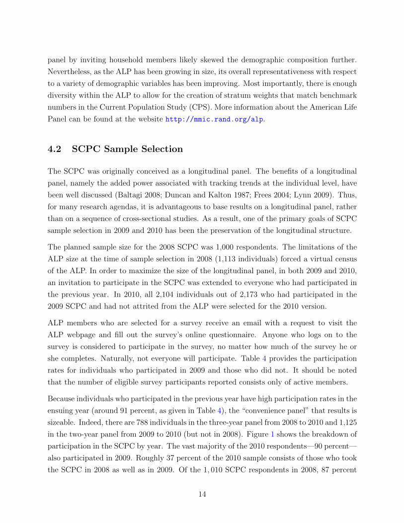
she completes. Naturally, not everyone will participate. Table 4 provides the participation

rates for individuals who participated in 2009 and those who did not. It should be noted

that the number of eligible survey participants reported consists only of active members.

Because individuals who participated in the previous year have high participation rates in the

ensuing year (around 91 percent, as given in Table 4), the “convenience panel” that results is

sizeable. Indeed, there are 788 individuals in the three-year panel from 2008 to 2010 and 1,125

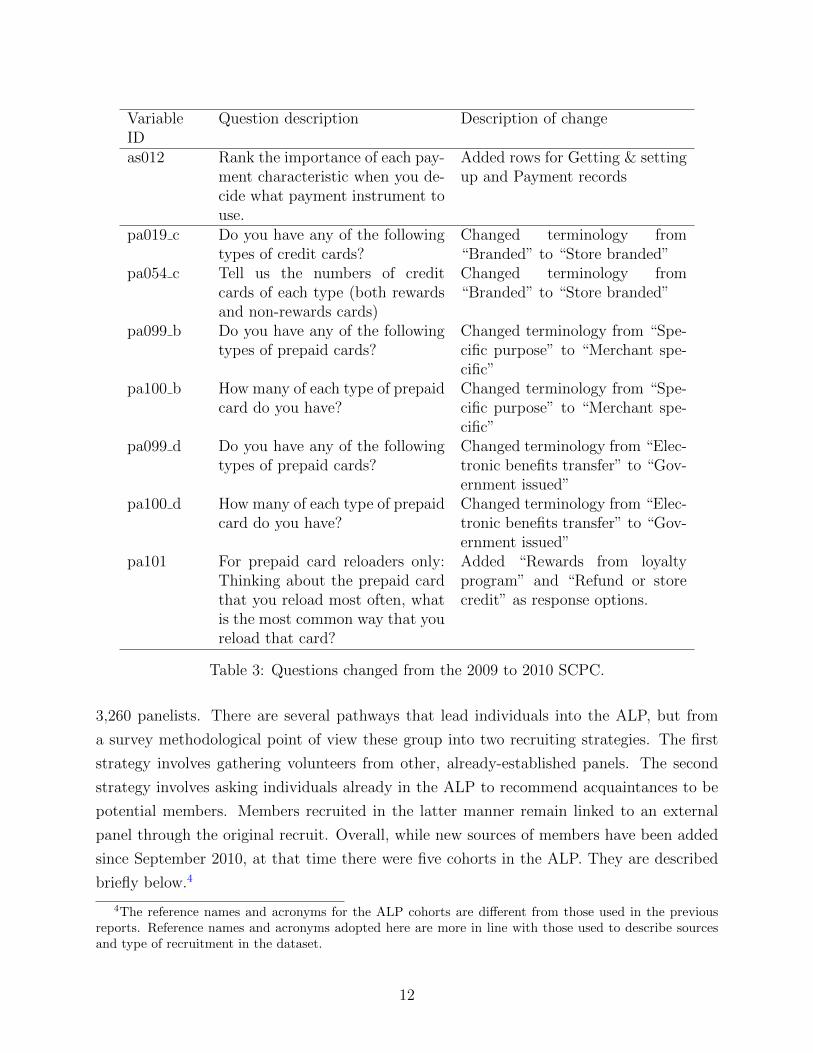
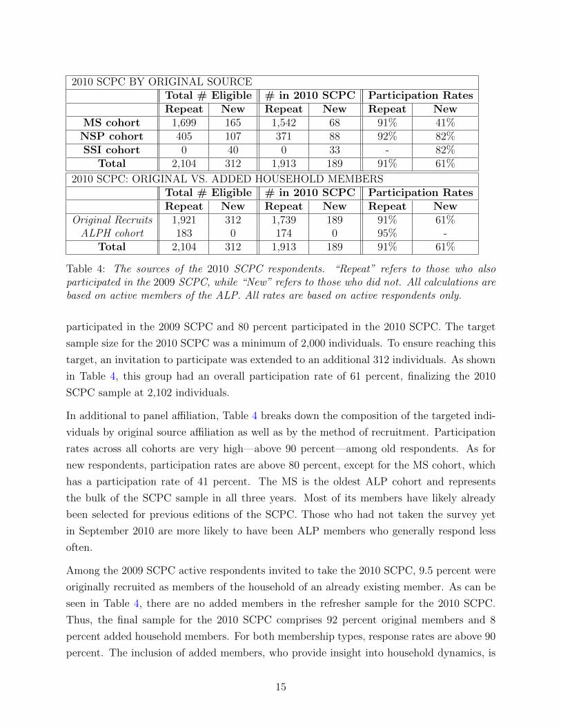
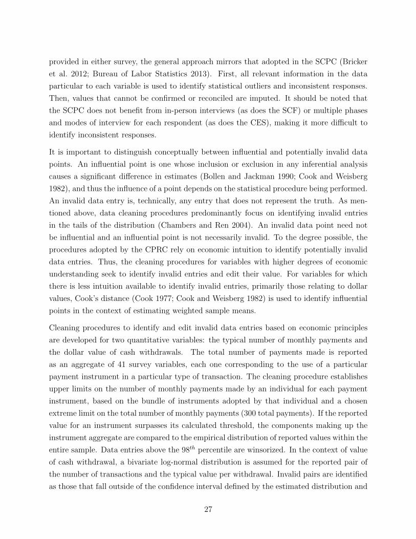
in the two-year panel from 2009 to 2010 (but not in 2008). Figure 1 shows the breakdown of

participation in the SCPC by year. The vast majority of the 2010 respondents—90 percent—

also participated in 2009. Roughly 37 percent of the 2010 sample consists of those who took

the SCPC in 2008 as well as in 2009. Of the 1, 010 SCPC respondents in 2008, 87 percent

14

2010 SCPC BY ORIGINAL SOURCETotal # Eligible # in 2010 SCPC Participation RatesRepeat New Repeat New Repeat New

MS cohort 1,699 165 1,542 68 91% 41%NSP cohort 405 107 371 88 92% 82%SSI cohort 0 40 0 33 - 82%

Total 2,104 312 1,913 189 91% 61%

2010 SCPC: ORIGINAL VS. ADDED HOUSEHOLD MEMBERSTotal # Eligible # in 2010 SCPC Participation RatesRepeat New Repeat New Repeat New

Original Recruits 1,921 312 1,739 189 91% 61%ALPH cohort 183 0 174 0 95% -

Total 2,104 312 1,913 189 91% 61%

Table 4: The sources of the 2010 SCPC respondents. “Repeat” refers to those who alsoparticipated in the 2009 SCPC, while “New” refers to those who did not. All calculations arebased on active members of the ALP. All rates are based on active respondents only.

participated in the 2009 SCPC and 80 percent participated in the 2010 SCPC. The target

sample size for the 2010 SCPC was a minimum of 2,000 individuals. To ensure reaching this

target, an invitation to participate was extended to an additional 312 individuals. As shown

in Table 4, this group had an overall participation rate of 61 percent, finalizing the 2010

SCPC sample at 2,102 individuals.

In additional to panel affiliation, Table 4 breaks down the composition of the targeted indi-

viduals by original source affiliation as well as by the method of recruitment. Participation

rates across all cohorts are very high—above 90 percent—among old respondents. As for

new respondents, participation rates are above 80 percent, except for the MS cohort, which

has a participation rate of 41 percent. The MS is the oldest ALP cohort and represents

the bulk of the SCPC sample in all three years. Most of its members have likely already

been selected for previous editions of the SCPC. Those who had not taken the survey yet

in September 2010 are more likely to have been ALP members who generally respond less

often.

Among the 2009 SCPC active respondents invited to take the 2010 SCPC, 9.5 percent were

originally recruited as members of the household of an already existing member. As can be

seen in Table 4, there are no added members in the refresher sample for the 2010 SCPC.

Thus, the final sample for the 2010 SCPC comprises 92 percent original members and 8

percent added household members. For both membership types, response rates are above 90

percent. The inclusion of added members, who provide insight into household dynamics, is

15

20

10

20

09

20

08

in all 3 years (788)in 2009 and 2010 only (1125)in 2008 and 2009 only (88)in 2008 and 2010 only (22)in 2008 only (112)in 2009 only (172)in 2010 only (167)

0 500 1000 1500 2000

Number of Respondents in Survey

Yea

r o

f S

urv

eyNumber and Overlap of Survey Respondents

2102

2173

1010

Figure 1: The annual composition of the SCPC respondents.

a valuable component of the SCPC for certain types of economic analysis.

The longitudinal panel is an important aspect of the annual survey, and further development

of its statistical properties is a high priority for future implementations. This process involves

systematically addressing attrition and panel member replacement, as well as developing a

methodology for the creation of longitudinal weights. Research into the latter is currently

being done at the CPRC, with the methodology based on that undertaken by the Panel Study

of Income Dynamics (Gouskova et al. 2008). At the moment, however, only cross-sectional

weights are provided with the dataset.5

4.3 Survey Completion

Each year, the SCPC is fielded in the fall with the goal of having most surveys completed in

the month of October. The desire to standardize this response period is two-fold. First, from

an analytical point of view, trends from year to year are more easily identified if differences

in behavior are not attributable to seasonal behavioral variation. Second, from an economic

5Readers interested in more details about the longitudinal panel and longitudinal sample weights shouldcontact Marcin Hitczenko at: Marcin.Hitczenko@bos.frb.org.

16

point of view, the month of October was chosen as a reasonably representative month with

respect to yearly payment behavior; there are no major holidays and it falls between summer

and winter. Although we ask respondents for responses in a “typical” month, it is possible

that recent behavior influences responses.

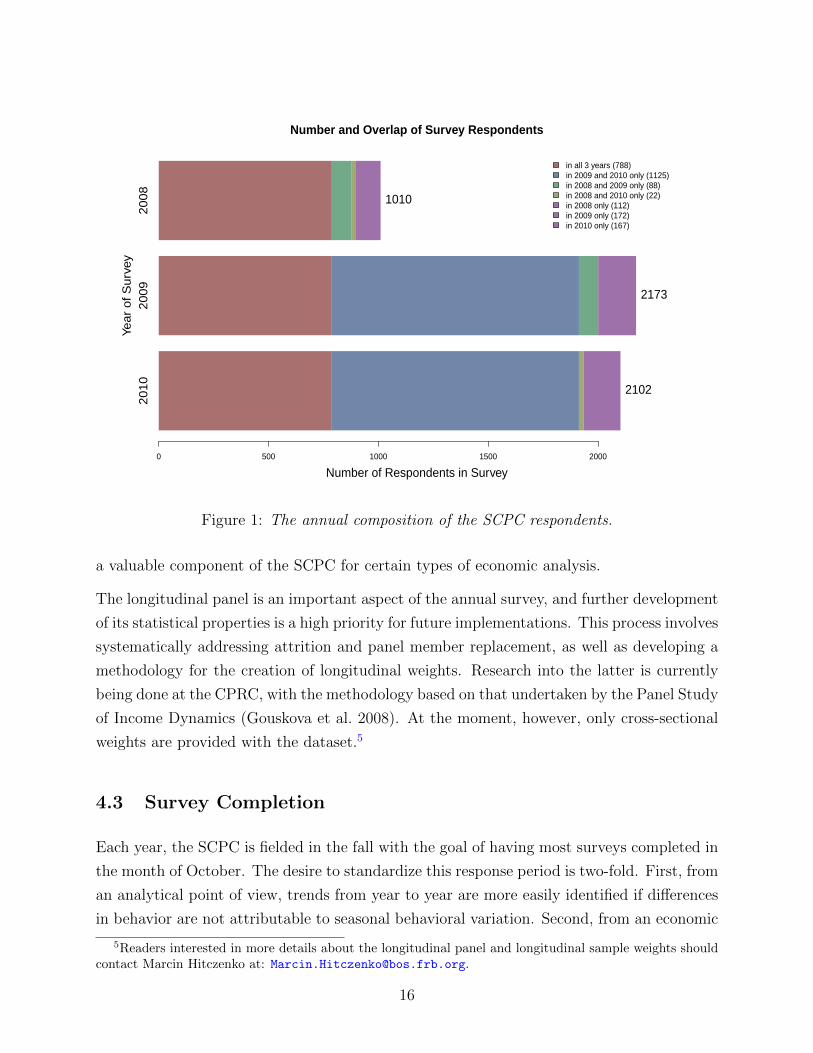
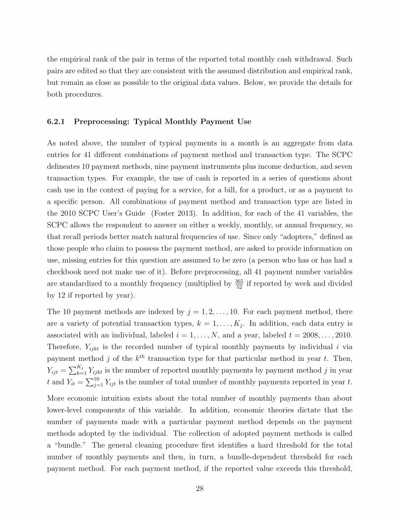
Despite this goal, the exact timing of the survey has varied across the years. The 2010 version

was released on September 29, 2010, over a month earlier than the 2009 version and a few

weeks later than the 2008 version. Figure 2 shows the proportion of surveys completed by

each calendar day within each of the three years. For this purpose, the date of completion is

defined to be the day on which the respondent logged off for the final time. It is important to

note that logging off may not accurately reflect total completion of the survey, as it is possible

to finish the survey without logging out. Other standards to define survey completion can

be used. For example, individuals who reached the last screen, which asks individuals for

feedback on the survey questionnaire itself, but did not log out also answered all of the

SCPC questions. Because our analysis utilizes data from everyone who ever participated

(logged on), these distinctions are not vital to further analysis or results. Item nonresponse

is addressed in Section 5.4.

While 1, 939 respondents (92 percent of the sample) completed the survey on the same day

they first logged on, and 133 (6.3 percent of the sample) completed the survey on a later

day, only 30 (1.4 percent of the sample) never logged off. The percentage of individuals who

never logged off is comparable for all three years.

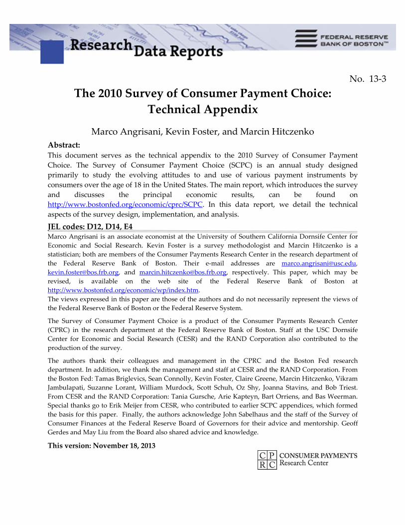
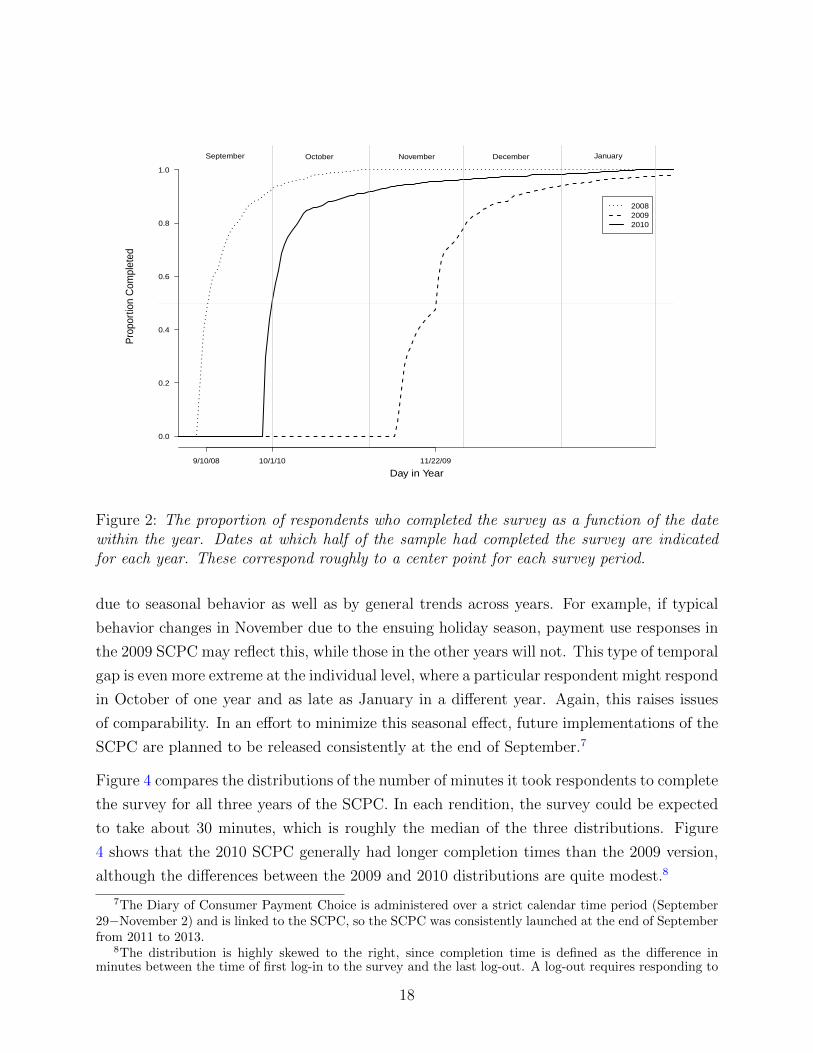
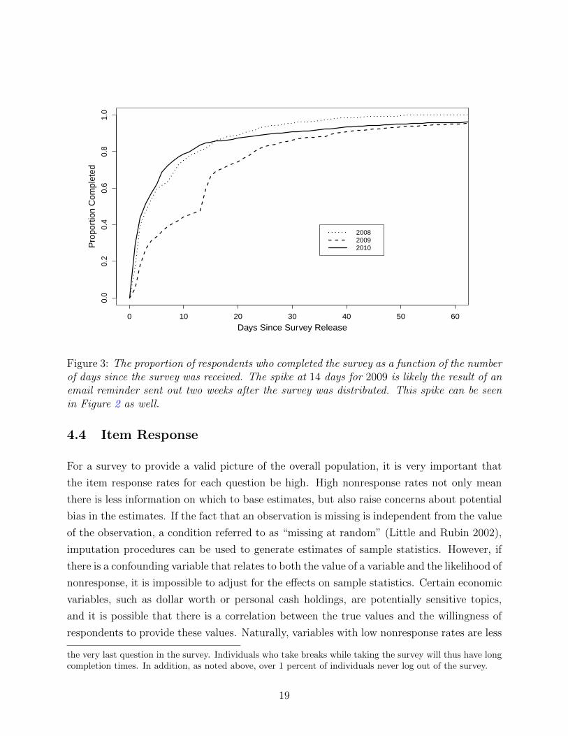
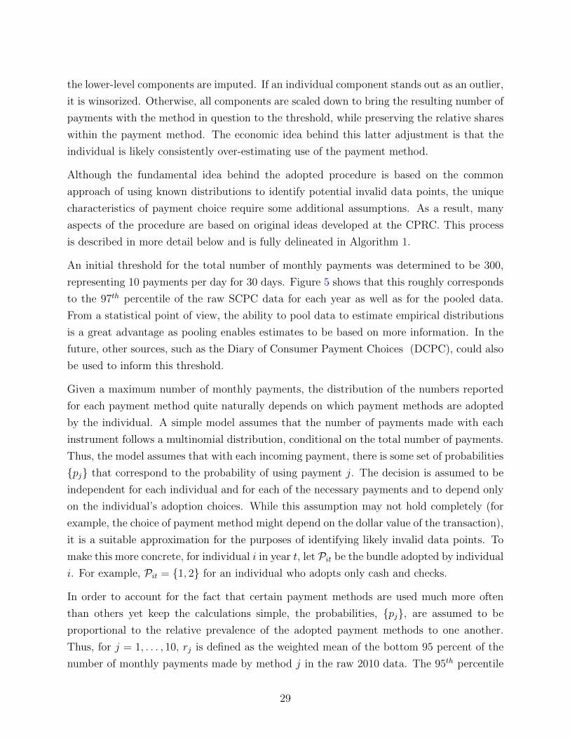
Figure 3, which shows the proportion of surveys completed as a function of the number of

days since the survey was distributed for the 2008, 2009, and 2010 versions, gives a better

sense of the distribution of days until completion. In 2010, over 50 percent of the respondents

had completed the survey within two days of its being made available, and 91 percent had

completed it within a month. This pattern is similar for the 2008 survey. In 2009, while 90

percent of the respondents had completed the survey after a month, only about 18 percent

had done so after a day.6

An important aspect of the SCPC time-series data made evident by the completion data

relates to the relatively wide range of dates within a year during which surveys are taken.

Approximately 80 percent of surveys are completed within two or three weeks of the release

date, as Figure 3 makes clear. Figure 2 shows that these periods do not overlap in the three

years of the SCPC. As a result, comparisons across years could be influenced by differences

6The 2009 SCPC went into the field on Tuesday, November 10th, 2009. The fact that the following daywas a public holiday (Veterans Day on November 11th, 2009) might explain why few respondents answeredthe survey after a day.

17

Day in Year

Pro

port

ion

Com

plet

ed

200820092010

9/10/08 10/1/10 11/22/09

0.0

0.2

0.4

0.6

0.8

1.0

September October November December January

Figure 2: The proportion of respondents who completed the survey as a function of the datewithin the year. Dates at which half of the sample had completed the survey are indicatedfor each year. These correspond roughly to a center point for each survey period.

due to seasonal behavior as well as by general trends across years. For example, if typical

behavior changes in November due to the ensuing holiday season, payment use responses in

the 2009 SCPC may reflect this, while those in the other years will not. This type of temporal

gap is even more extreme at the individual level, where a particular respondent might respond

in October of one year and as late as January in a different year. Again, this raises issues

of comparability. In an effort to minimize this seasonal effect, future implementations of the

SCPC are planned to be released consistently at the end of September.7

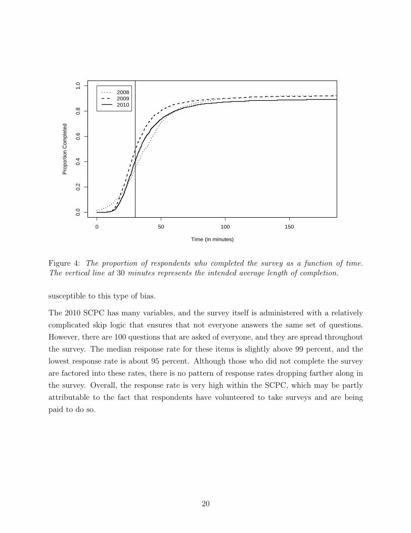
Figure 4 compares the distributions of the number of minutes it took respondents to complete

the survey for all three years of the SCPC. In each rendition, the survey could be expected

to take about 30 minutes, which is roughly the median of the three distributions. Figure

4 shows that the 2010 SCPC generally had longer completion times than the 2009 version,

although the differences between the 2009 and 2010 distributions are quite modest.8

7The Diary of Consumer Payment Choice is administered over a strict calendar time period (September29−November 2) and is linked to the SCPC, so the SCPC was consistently launched at the end of Septemberfrom 2011 to 2013.

8The distribution is highly skewed to the right, since completion time is defined as the difference inminutes between the time of first log-in to the survey and the last log-out. A log-out requires responding to

18

0 10 20 30 40 50 60

0.0

0.2

0.4

0.6

0.8

1.0

Days Since Survey Release

Pro

port

ion

Com

plet

ed

200820092010

Figure 3: The proportion of respondents who completed the survey as a function of the numberof days since the survey was received. The spike at 14 days for 2009 is likely the result of anemail reminder sent out two weeks after the survey was distributed. This spike can be seenin Figure 2 as well.

4.4 Item Response

For a survey to provide a valid picture of the overall population, it is very important that

the item response rates for each question be high. High nonresponse rates not only mean

there is less information on which to base estimates, but also raise concerns about potential

bias in the estimates. If the fact that an observation is missing is independent from the value

of the observation, a condition referred to as “missing at random” (Little and Rubin 2002),

imputation procedures can be used to generate estimates of sample statistics. However, if

there is a confounding variable that relates to both the value of a variable and the likelihood of

nonresponse, it is impossible to adjust for the effects on sample statistics. Certain economic

variables, such as dollar worth or personal cash holdings, are potentially sensitive topics,

and it is possible that there is a correlation between the true values and the willingness of

respondents to provide these values. Naturally, variables with low nonresponse rates are less

the very last question in the survey. Individuals who take breaks while taking the survey will thus have longcompletion times. In addition, as noted above, over 1 percent of individuals never log out of the survey.

19

0 50 100 150

0.0

0.2

0.4

0.6

0.8

1.0

Time (in minutes)

Pro

port

ion

Com

plet

ed

200820092010

Figure 4: The proportion of respondents who completed the survey as a function of time.The vertical line at 30 minutes represents the intended average length of completion.

susceptible to this type of bias.

The 2010 SCPC has many variables, and the survey itself is administered with a relatively

complicated skip logic that ensures that not everyone answers the same set of questions.

However, there are 100 questions that are asked of everyone, and they are spread throughout

the survey. The median response rate for these items is slightly above 99 percent, and the

lowest response rate is about 95 percent. Although those who did not complete the survey

are factored into these rates, there is no pattern of response rates dropping farther along in

the survey. Overall, the response rate is very high within the SCPC, which may be partly

attributable to the fact that respondents have volunteered to take surveys and are being

paid to do so.

20

5 Sampling Weights

5.1 Post-Stratification

An important goal of the SCPC is to provide estimates of payment statistics for the entire

population of U.S. consumers over the age of 18. As mentioned in Section 4, the ALP

is a collection of volunteers from several other samples and in some respects may not be

representative of the population. In addition, because the SCPC has focused on preserving

the longitudinal aspect of the sample and the 2008 sample was based on a virtual census

of the ALP, the SCPC sample itself is not necessarily representative of the U.S. population

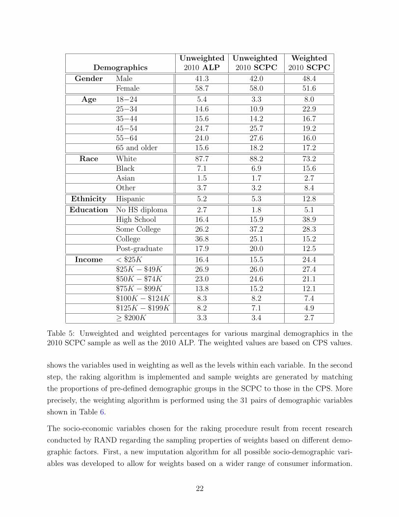
of consumers. Table 5 shows the unweighted sample proportions for various demographic

categories along with the weighted ones. It is clear that the SCPC tends to under-sample

males as well as young people, minorities, people with lower levels of education, and those

with lower income levels.

To enable better inference of the entire population of U.S. consumers, SCPC respondents are

assigned post-stratified survey weights designed to align as much as possible the composition

of the SCPC sample to that of a reference population. Specifically, each year the benchmark

distributions against which SCPC surveys are weighted are derived from the Current Popu-

lation Survey Annual Social and Economic Supplement, administered in March (CPS). This

follows common practice in other social science surveys, such as the Consumer Expenditure

Survey (CES).

5.2 Raking Algorithm

Sampling weights are generated by RAND, using a raking algorithm (Deming and Stephan

1940; Gelman and Lu 2003). This iterative process assigns a weight to each respondent so

that the weighted distributions of specific socio-demographic variables in the SCPC sample

match their population counterparts (benchmark or target distributions). The weighting

procedure consists of two main steps. In the first part, demographic variables from the CPS

are chosen and mapped onto those available in the SCPC. Continuous variables such as age

and income are recoded as categorical variables by assigning each to one of several disjoint

intervals. For example, Table 5 shows six classifications for age and seven classifications

for income. The number of levels for each variable should be small enough to capture

homogeneity within each level, but large enough to prevent strata containing a very small

fraction of the sample, which could cause weights to exhibit considerable variability. Table 6

21

Unweighted Unweighted WeightedDemographics 2010 ALP 2010 SCPC 2010 SCPC

Gender Male 41.3 42.0 48.4Female 58.7 58.0 51.6

Age 18−24 5.4 3.3 8.025−34 14.6 10.9 22.935−44 15.6 14.2 16.745−54 24.7 25.7 19.255−64 24.0 27.6 16.065 and older 15.6 18.2 17.2

Race White 87.7 88.2 73.2Black 7.1 6.9 15.6Asian 1.5 1.7 2.7Other 3.7 3.2 8.4

Ethnicity Hispanic 5.2 5.3 12.8

Education No HS diploma 2.7 1.8 5.1High School 16.4 15.9 38.9Some College 26.2 37.2 28.3College 36.8 25.1 15.2Post-graduate 17.9 20.0 12.5

Income < $25K 16.4 15.5 24.4$25K − $49K 26.9 26.0 27.4$50K − $74K 23.0 24.6 21.1$75K − $99K 13.8 15.2 12.1$100K − $124K 8.3 8.2 7.4$125K − $199K 8.2 7.1 4.9≥ $200K 3.3 3.4 2.7

Table 5: Unweighted and weighted percentages for various marginal demographics in the2010 SCPC sample as well as the 2010 ALP. The weighted values are based on CPS values.

shows the variables used in weighting as well as the levels within each variable. In the second

step, the raking algorithm is implemented and sample weights are generated by matching

the proportions of pre-defined demographic groups in the SCPC to those in the CPS. More

precisely, the weighting algorithm is performed using the 31 pairs of demographic variables

shown in Table 6.

The socio-economic variables chosen for the raking procedure result from recent research

conducted by RAND regarding the sampling properties of weights based on different demo-

graphic factors. First, a new imputation algorithm for all possible socio-demographic vari-

ables was developed to allow for weights based on a wider range of consumer information.

22

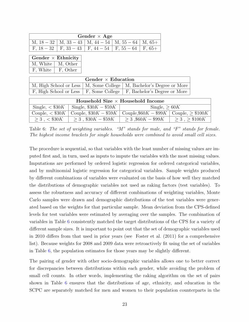
Gender × AgeM, 18− 32 M, 33− 43 M, 44− 54 M, 55− 64 M, 65+F, 18− 32 F, 33− 43 F, 44− 54 F, 55− 64 F, 65+

Gender × EthnicityM, White M, OtherF, White F, Other

Gender × EducationM, High School or Less M, Some College M, Bachelor’s Degree or MoreF, High School or Less F, Some College F, Bachelor’s Degree or More

Household Size × Household IncomeSingle, < $30K Single, $30K − $59K Single, ≥ 60KCouple, < $30K Couple, $30K − $59K Couple,$60K − $99K Couple, ≥ $100K≥ 3 , < $30K ≥ 3 , $30K − $59K ≥ 3 ,$60K − $99K ≥ 3 , ≥ $100K

Table 6: The set of weighting variables. “M” stands for male, and “F” stands for female.The highest income brackets for single households were combined to avoid small cell sizes.

The procedure is sequential, so that variables with the least number of missing values are im-

puted first and, in turn, used as inputs to impute the variables with the most missing values.

Imputations are performed by ordered logistic regression for ordered categorical variables,

and by multinomial logistic regression for categorical variables. Sample weights produced

by different combinations of variables were evaluated on the basis of how well they matched

the distributions of demographic variables not used as raking factors (test variables). To

assess the robustness and accuracy of different combinations of weighting variables, Monte

Carlo samples were drawn and demographic distributions of the test variables were gener-

ated based on the weights for that particular sample. Mean deviation from the CPS-defined

levels for test variables were estimated by averaging over the samples. The combination of

variables in Table 6 consistently matched the target distributions of the CPS for a variety of

different sample sizes. It is important to point out that the set of demographic variables used

in 2010 differs from that used in prior years (see Foster et al. (2011) for a comprehensive

list). Because weights for 2008 and 2009 data were retroactively fit using the set of variables

in Table 6, the population estimates for those years may be slightly different.

The pairing of gender with other socio-demographic variables allows one to better correct

for discrepancies between distributions within each gender, while avoiding the problem of

small cell counts. In other words, implementing the raking algorithm on the set of pairs

shown in Table 6 ensures that the distributions of age, ethnicity, and education in the

SCPC are separately matched for men and women to their population counterparts in the

23

CPS. Moreover, since bivariate distributions imply marginal distributions for each of the two

variables, this approach also guarantees that the distributions of gender, age, ethnicity, and

education for the entire SCPC sample are aligned with the corresponding benchmarks in the

CPS. The same is true for household size and household income.

Because the ALP sample itself is not representative of the U.S. population, post-stratification

is an important step in inference for the population. The fact that not all strata of interest are

represented in the sample makes raking the natural method for assigning weights. However,

doing so introduces a few complications related to the statistical framework and analysis

of the data. The first relates to the increased difficulty in calculating standard errors of

population estimates, which are weighted averages of the sample values. In all tables and

publications, the standard errors have been calculated by taking the weights as fixed values,

thereby reducing the standard errors. The sampling weights, which are a function of the

strata representation in the sample, are random variables, and their variation should be

factored into the calculation of standard errors (Gelman and Lu 2003).

The second area of concern regards the effects of the sampling scheme on the weights and

on the estimates they produce. In order for the raking algorithm to be appropriate, in the

sense that the expected weights for each stratum equal those of the population, the sampling

procedure must be such that, in expectation, each stratum is proportionally represented in

the sample. To be precise, the expected proportion of the sample belonging to a specific

stratum is directly proportional to the relative proportion of that stratum within the pop-

ulation. A sampling procedure that does not have this property is likely to consistently

produce weights for certain strata that do not reflect the true representation in the entire

population. If strata properties correlate with payment behavior, this could lead to biased

population-wide estimates. In the case of a sampling procedure in which some strata tend

to be over-represented and others under-represented, the raking algorithm, which strives to

match marginal proportions rather than those of the cross-sections of all the variables, may

generate sample weights with too wide a range of values in order to achieve the alignment

between the sample composition and the one in the reference population. Work is currently

being done to better incorporate CPS population proportions for strata into the sampling

scheme in the hope of eliminating any potential bias from nonproportional stratum sampling.

Despite these issues, the results of the SCPC data and any observed changes from year

to year based on these results are likely to be reliable. High response rates and targeted

sampling (as described in Section 3.2) suggest that the variability in estimates attributable

to the weights is relatively small. In addition, there is little evidence of strong correlations

between demographic variables and consumer behavior, with a lot of the variation seen in

24

the data seemingly attributable to differences from person to person at the individual level.

This suggests that mis-specification of weights would have a minor impact on any point

estimates and likely result in conservative confidence intervals. Such intervals, in turn, make

Type-I errors less likely, suggesting any trends we do see in the data are real. A discussion

of using the post-stratification weights to generate per-consumer as well as aggregate U.S.

population estimates is found in Section 7.2.1.

6 Data Preprocessing

Prior to further statistical analysis, it is important to carefully examine the data and develop

a consistent methodology for dealing with potentially invalid and influential data points. As

a survey that gathers a large range of information from each respondent, much of it about a

rather technical aspect of life that people may not be used to thinking about in such detail,

the SCPC, like any consumer survey, is susceptible to erroneous input or missing values. This

section describes the general types of data preprocessing issues encountered in the SCPC

and outlines the general philosophy in data cleaning. The details of the data cleaning and

editing procedure for two distinct types of survey variables are provided in Section 6.2.1 and

Section 6.2.2. It should be noted that the newly devised procedures are also applied to the

data of previous years, so survey variables from 2008 and 2009 may have different values

from those in previous data releases.

6.1 Categorical Data

It is worth distinguishing the preprocessing of categorical data from the preprocessing of

quantitative data, as the issues and strategies differ substantially between the two. The

types of categorical variables in the SCPC are diverse, ranging from demographic variables, to

binary variables (answers to Yes/No questions), to polytomous response variables (multiple

choice questions with more than two possible answers). The first line of data inspection

consists of a basic range and consistency check for the demographic variables to ensure that

reported values are logical and that they correspond to established categorical codes. Any

response item that fails this check is considered to be missing data.

Treatment of demographic variables differs from treatment of all other categorical variables.

In the case of many demographic variables, such as age group, gender, or race, missing

information can be verified from other surveys taken within the context of the ALP. For

25

household income and household size, both attributes that could easily change within a

year, values are imputed through logistic regression models for the purpose of creating post-

stratification weights by RAND. At the moment, no other variables are imputed, although

multiple imputation procedures are being planned for future editions of the survey results.

Nondemographic categorical variables are neither changed from their original values nor

imputed if missing. These are most often obtained in response to a binary question (“Have

you ever had a credit card?”) or in response to questions asking the subject to rate a

variety of characteristics for different payment instruments on a Likert scale. It is very

difficult, without making strong assumptions, to identify irregular or erroneous data inputs.

Therefore, responses to multiple choice questions are not changed. However, the CPRC is

conducting research into correcting for possible response bias in sequences of Likert scale

questions introduced by a form of anchoring effects (Hitczenko (2013a), see Daamen and

de Bie (1992); Friedman, Herskovitz, and Pollack (1994) for general discussion on anchoring

effects). Because the item response rates are high, the effect of missing values is not a major

concern for the SCPC. Nevertheless, the CPRC is working to develop multiple imputation

techniques for missing data entries.

6.2 Quantitative Data

The greatest challenge in data preprocessing for the SCPC comes in the form of quantitative

variables, especially those that represent the number of monthly payments or dollar values.

Measurement errors in such a context, defined as any incongruity between the data entry

and the true response, can be attributed to a variety of sources ranging from recall error to

rounding errors to data entry errors or even to misinterpretation of the question. A data

entry subject to measurement error can take many forms, but practically the only identifiable

forms are those that lie outside the realm of possible values and those that fall in the realm of

possibility, but take extreme values. The former, such as negative monthly payment counts,

are easily identified by range checks. Identification of the latter is much more difficult, as it

is important to recognize the heterogeneity of behavior within the population, especially for

economic variables such as cash holdings and value of assets. In other words, it is possible

that data entries that by some numerical evaluations are statistical outliers are actually

accurate and valid.

This issue is not unique to the SCPC. Many consumer surveys, such as the Survey of Con-

sumer Finances (SCF) and the Consumer Expenditure Survey (CES) must also tackle the

cleaning of such fat-tailed variables. While the details of the preprocessing of outliers are not

26

provided in either survey, the general approach mirrors that adopted in the SCPC (Bricker

et al. 2012; Bureau of Labor Statistics 2013). First, all relevant information in the data

particular to each variable is used to identify statistical outliers and inconsistent responses.

Then, values that cannot be confirmed or reconciled are imputed. It should be noted that

the SCPC does not benefit from in-person interviews (as does the SCF) or multiple phases

and modes of interview for each respondent (as does the CES), making it more difficult to

identify inconsistent responses.

It is important to distinguish conceptually between influential and potentially invalid data

points. An influential point is one whose inclusion or exclusion in any inferential analysis

causes a significant difference in estimates (Bollen and Jackman 1990; Cook and Weisberg

1982), and thus the influence of a point depends on the statistical procedure being performed.

An invalid data entry is, technically, any entry that does not represent the truth. As men-

tioned above, data cleaning procedures predominantly focus on identifying invalid entries

in the tails of the distribution (Chambers and Ren 2004). An invalid data point need not

be influential and an influential point is not necessarily invalid. To the degree possible, the

procedures adopted by the CPRC rely on economic intuition to identify potentially invalid

data entries. Thus, the cleaning procedures for variables with higher degrees of economic

understanding seek to identify invalid entries and edit their value. For variables for which

there is less intuition available to identify invalid entries, primarily those relating to dollar

values, Cook’s distance (Cook 1977; Cook and Weisberg 1982) is used to identify influential

points in the context of estimating weighted sample means.

Cleaning procedures to identify and edit invalid data entries based on economic principles

are developed for two quantitative variables: the typical number of monthly payments and

the dollar value of cash withdrawals. The total number of payments made is reported

as an aggregate of 41 survey variables, each one corresponding to the use of a particular

payment instrument in a particular type of transaction. The cleaning procedure establishes

upper limits on the number of monthly payments made by an individual for each payment

instrument, based on the bundle of instruments adopted by that individual and a chosen

extreme limit on the total number of monthly payments (300 total payments). If the reported

value for an instrument surpasses its calculated threshold, the components making up the

instrument aggregate are compared to the empirical distribution of reported values within the

entire sample. Data entries above the 98th percentile are winsorized. In the context of value

of cash withdrawal, a bivariate log-normal distribution is assumed for the reported pair of

the number of transactions and the typical value per withdrawal. Invalid pairs are identified

as those that fall outside of the confidence interval defined by the estimated distribution and

27

the empirical rank of the pair in terms of the reported total monthly cash withdrawal. Such

pairs are edited so that they are consistent with the assumed distribution and empirical rank,

but remain as close as possible to the original data values. Below, we provide the details for

both procedures.

6.2.1 Preprocessing: Typical Monthly Payment Use

As noted above, the number of typical payments in a month is an aggregate from data

entries for 41 different combinations of payment method and transaction type. The SCPC

delineates 10 payment methods, nine payment instruments plus income deduction, and seven

transaction types. For example, the use of cash is reported in a series of questions about

cash use in the context of paying for a service, for a bill, for a product, or as a payment to

a specific person. All combinations of payment method and transaction type are listed in

the 2010 SCPC User’s Guide (Foster 2013). In addition, for each of the 41 variables, the

SCPC allows the respondent to answer on either a weekly, monthly, or annual frequency, so

that recall periods better match natural frequencies of use. Since only “adopters,” defined as

those people who claim to possess the payment method, are asked to provide information on

use, missing entries for this question are assumed to be zero (a person who has or has had a

checkbook need not make use of it). Before preprocessing, all 41 payment number variables

are standardized to a monthly frequency (multiplied by 36552

if reported by week and divided

by 12 if reported by year).

The 10 payment methods are indexed by j = 1, 2, . . . , 10. For each payment method, there

are a variety of potential transaction types, k = 1, . . . , Kj. In addition, each data entry is

associated with an individual, labeled i = 1, . . . , N , and a year, labeled t = 2008, . . . , 2010.

Therefore, Yijkt is the recorded number of typical monthly payments by individual i via

payment method j of the kth transaction type for that particular method in year t. Then,

Yijt =∑Kj

k=1 Yijkt is the number of reported monthly payments by payment method j in year

t and Yit =∑10

j=1 Yijt is the number of total number of monthly payments reported in year t.

More economic intuition exists about the total number of monthly payments than about

lower-level components of this variable. In addition, economic theories dictate that the

number of payments made with a particular payment method depends on the payment

methods adopted by the individual. The collection of adopted payment methods is called

a “bundle.” The general cleaning procedure first identifies a hard threshold for the total

number of monthly payments and then, in turn, a bundle-dependent threshold for each

payment method. For each payment method, if the reported value exceeds this threshold,

28

the lower-level components are imputed. If an individual component stands out as an outlier,

it is winsorized. Otherwise, all components are scaled down to bring the resulting number of

payments with the method in question to the threshold, while preserving the relative shares

within the payment method. The economic idea behind this latter adjustment is that the

individual is likely consistently over-estimating use of the payment method.

Although the fundamental idea behind the adopted procedure is based on the common

approach of using known distributions to identify potential invalid data points, the unique

characteristics of payment choice require some additional assumptions. As a result, many

aspects of the procedure are based on original ideas developed at the CPRC. This process

is described in more detail below and is fully delineated in Algorithm 1.

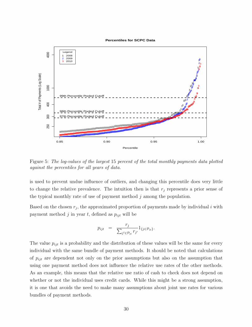
An initial threshold for the total number of monthly payments was determined to be 300,

representing 10 payments per day for 30 days. Figure 5 shows that this roughly corresponds

to the 97th percentile of the raw SCPC data for each year as well as for the pooled data.

From a statistical point of view, the ability to pool data to estimate empirical distributions

is a great advantage as pooling enables estimates to be based on more information. In the

future, other sources, such as the Diary of Consumer Payment Choices (DCPC), could also

be used to inform this threshold.

Given a maximum number of monthly payments, the distribution of the numbers reported

for each payment method quite naturally depends on which payment methods are adopted

by the individual. A simple model assumes that the number of payments made with each

instrument follows a multinomial distribution, conditional on the total number of payments.

Thus, the model assumes that with each incoming payment, there is some set of probabilities

{pj} that correspond to the probability of using payment j. The decision is assumed to be

independent for each individual and for each of the necessary payments and to depend only

on the individual’s adoption choices. While this assumption may not hold completely (for

example, the choice of payment method might depend on the dollar value of the transaction),

it is a suitable approximation for the purposes of identifying likely invalid data points. To

make this more concrete, for individual i in year t, let Pit be the bundle adopted by individual

i. For example, Pit = {1, 2} for an individual who adopts only cash and checks.

In order to account for the fact that certain payment methods are used much more often

than others yet keep the calculations simple, the probabilities, {pj}, are assumed to be

proportional to the relative prevalence of the adopted payment methods to one another.

Thus, for j = 1, . . . , 10, rj is defined as the weighted mean of the bottom 95 percent of the

number of monthly payments made by method j in the raw 2010 data. The 95th percentile

29

Percentiles for SCPC Data

Percentile

Tota

l # o

f Pay

men

ts (L

og S

cale

)

0.85 0.90 0.95 1.00

250

300

400

1000

4000

11

1

11

1111

11

1

111

111

11

11

1111111111111111111111111111111111111111111111111111111111111111111111111111111111111111111111111111111111111111111111111111111

22

2

2

2222

22222222

22222

2222222222

222222

2222222222222222222222222222222222222222222222222222222222222222222222222222222222222222222222222222222222222222222222222222222222222222222222222222222222222222222222222222222222222222222222222222222222222222222222222222222222222222222222222222222222222222222222222222222222222222222222

333

3

333

333333

333

33333333333333333333333333333333333333333333333333333333333333333333333333333333333333333333333333333333333333333333333333333333333333333333333333333333333333333333333333333333333333333333333333333333333333333333333333333333333333333333333333333333333333333333333333333333333333333333333333333333

99th Percentile Pooled Cutoff

98th Percentile Pooled Cutoff

97th Percentile Pooled Cutoff

123

Legend

200820092010

Figure 5: The log-values of the largest 15 percent of the total monthly payments data plottedagainst the percentiles for all years of data.

is used to prevent undue influence of outliers, and changing this percentile does very little

to change the relative prevalence. The intuition then is that rj represents a prior sense of

the typical monthly rate of use of payment method j among the population.

Based on the chosen rj, the approximated proportion of payments made by individual i with

payment method j in year t, defined as pijt will be

pijt =rj∑

j′∈Pitrj′

1{j∈Pit}.

The value pijt is a probability and the distribution of these values will be the same for every

individual with the same bundle of payment methods. It should be noted that calculations

of pijt are dependent not only on the prior assumptions but also on the assumption that

using one payment method does not influence the relative use rates of the other methods.

As an example, this means that the relative use ratio of cash to check does not depend on

whether or not the individual uses credit cards. While this might be a strong assumption,

it is one that avoids the need to make many assumptions about joint use rates for various

bundles of payment methods.

30

The cutoffs for each payment method are then defined as the 98th percentile of the number

of monthly payments, with 300 total payments and probability of use pijt. Therefore, if

Yijt ∼ Binomial(300, pijt), the cutoff cijt is defined to be such that

Prob(Yijt ≤ cijt) = 0.98.

Based on this, yijt is flagged whenever yijt > cijt. This flag indicates that the reported value

is unusually high when taking into account the payment methods adopted. It is only at this

point that the lowest level of data entry, yijkt, is studied. Because little intuition exists about

the distributions of the yijkt, comparisons of flagged values are made to the 98th percentile of

the empirical distribution estimated by pooling data from all three years. Specifically, let qjk

be the 98th percentile of the pooled set of data comprised of the yijkt for t = 2008, 2009, 2010

among people for all (i, t) for which j ∈ Pit. Then, for each flagged payment method, the

flagged entry is imputed with the minimum of the calculated quantile and the entered value:

y∗ijkt = min(yijkt, qjk). This form of winsorizing means that extremely high reported numbers

are brought down to still high, but reasonable levels. If none of the data entries at the lowest

level is changed, all yijkt for the payment method j are scaled down proportionally in order

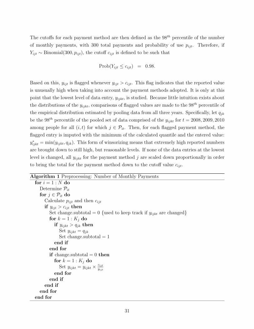
to bring the total for the payment method down to the cutoff value cijt.

Algorithm 1 Preprocessing: Number of Monthly Payments

for i = 1 : N doDetermine Pitfor j ∈ Pit do

Calculate pijt and then cijtif yijt > cijt then

Set change.subtotal = 0 {used to keep track if yijkt are changed}for k = 1 : Kj do

if yijkt > qjk thenSet yijkt = qjkSet change.subtotal = 1

end ifend forif change.subtotal = 0 then

for k = 1 : Kj doSet yijkt = yijkt × cijt

yijt

end forend if

end ifend for

end for

31

6.2.2 Preprocessing: Cash Withdrawal

Besides the number of monthly payments, the data variable that requires the most attention

in terms of preprocessing is that of cash withdrawal. Cash withdrawal in the 2009 and 2010

SCPC is reported as a combination of four separate variables: frequency of withdrawal at

primary and all other locations and typical dollar amount per withdrawal at primary and all

other locations. Because reported dollar amounts correspond to typical values, which could

correspond to the mean, the median, or the mode, the value determined by multiplying the

reported frequency and the dollar amount does not necessarily correspond to the average

total cash withdrawal either for primary or for all other locations. In preprocessing the cash

withdrawal values, data for primary and all other locations are treated separately.

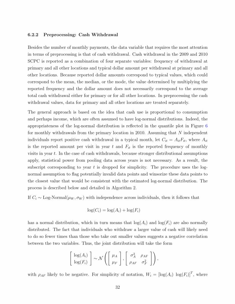
The general approach is based on the idea that cash use is proportional to consumption

and perhaps income, which are often assumed to have log-normal distributions. Indeed, the

appropriateness of the log-normal distribution is reflected in the quantile plot in Figure 6

for monthly withdrawals from the primary location in 2010. Assuming that N independent

individuals report positive cash withdrawal in a typical month, let Cit = AitFit, where Ait

is the reported amount per visit in year t and Fit is the reported frequency of monthly

visits in year t. In the case of cash withdrawals, because stronger distributional assumptions

apply, statistical power from pooling data across years is not necessary. As a result, the

subscript corresponding to year t is dropped for simplicity. The procedure uses the log-

normal assumption to flag potentially invalid data points and winsorize these data points to

the closest value that would be consistent with the estimated log-normal distribution. The

process is described below and detailed in Algorithm 2.

If Ci ∼ Log-Normal(µW , σW ) with independence across individuals, then it follows that

log(Ci) = log(Ai) + log(Fi)

has a normal distribution, which in turn means that log(Ai) and log(Fi) are also normally

distributed. The fact that individuals who withdraw a larger value of cash will likely need

to do so fewer times than those who take out smaller values suggests a negative correlation

between the two variables. Thus, the joint distribution will take the form[log(Ai)

log(Fi)

]∼ N

([µA

µF

],

[σ2A ρAF

ρAF σ2F

]),

with ρAF likely to be negative. For simplicity of notation, Wi = [log(Ai) log(Fi)]T , where

32

●

●

●

●

●

●

●

●

●

●

●

●

●

●

●

●

●

●

●

●

●

●

●

●

●

●

●

●

●

●

●

●

●

●

●

●

●

●

●

●

●●●

●

●

●

●●

●

●

●

●

●

●

●

●

●

●

●

●

●

●

●

●

●

●

●

●

●

●

●●

●

●

●

●

●

●

●

●

●

●

●

●

●

●

●

●

●

●

●

●

●●

●

●●

●

●

●

●

●

●

●

●

●●●

●

●

●

●

●

●●

●

●

●

●●

●

● ●

●●

●

●

●

●

●

●

●

●

●

●

●

●●

●●

●

●

●

●

●

●●

●

●

●

●

●●

●

●

●

●

●

●

●

●

●

●●

●

●

●

●

●

●

●

●

●

●

●

●●

●

●

●

●

●

●

●

●●

●

●●●

●

●

●

●

●

●

●

●

●

●

●

●

●

●

●

●

●

●

●

●●

●

●

●

●

●

●

●

●

●

●●

●

● ●

●

●

●●

●

●

●

●

●

●●

●

●

●

●

●

●

●

●

●

●

●

●●

●

●

●

●

●

●

●

●

●

●

●

●

●

●

●

●

●

●

●

●

●

●

●

●

●

●

●●

●

●

●

●

●●

● ●

●

●

●

●

●

●

●

●

●

●

●

●

●

●

●

●●

●

●

●

●

●

●

●

●

●

●

●

●●

●

●

●

●

●

●

●

●●

●

●

●

●

●

●

●

●

●

●

●

●

●

●●

●

●

●

●

●

●

●

●

●

●

●

●

●

●

●

●●

●

●

●●

●

●

●●

●

●●

●

●

●

●

●

●

●

●

●

●●●

●

●

●

●

●

●

●

●●

●

●

●

●

●●

●

●

●

●

●●

●

●

●

●

●

●

●

●

●●

●●

●

●

●

●

●

●

●

●

●

●

●

●

●

●

●

●

●

●

●

●

●

●

●

●

●

●

●●

●

●

●

●

●

●

●

●

●

●

●●

●

●

●

●

●

●

●

●

●●

●

●

● ●

●●

●

●

●

●

●

●

●●

●

●

●

●

●

●

●●

●●

●

●

●

●

●

●

●

●

●

●

●

●●

●

●

●

●●

●

●

●

●●

● ●

●

● ●

●

●

●

●

●

●

●

●

●

●

●

●

●

●

●

●

●

●

●

●

●

●

●

●

●

●

●

●

●

●

●

●

●

●

●

●

●

●

●

●

●

●

●

●

●

●

●

●

●

●

●

●

●

●

●

●

●

●

●

●

●

●●

●

●

●

●

●

●

●

●

●

●

●

●

●

●

●●

● ●

●

●

●

●

●

●

●

●

●

●

●

●●

●

●

●

●

●

●

●

●

●

●

●

●

●●

●

●

●

●

●

●

●

●

●

●

●

●

●

●

●

●

●

●

●

●

●

●

●

●

●

●

●

●

●

●

●

●

●

●

●

●

●

●

●●

●

●

●

●●

●

●

●

●

●

●

●

●

●●

●●

●

●

●

● ●

●

●●

●

●

●

●

●

●

●

●

●

●

●

●

●

●

●

●

●

●

●

●

●

●●

●

●

●

●

●

●

●

●

●

●

●

●

●

●

●

●

●

●●

●

●

●

●

●●

●

●

●

●

●

●

●

●●●

●

●

●

●

●

●●●

●

●●

●

●

●●

●

●

●●

●

●

●

●

●●

●

●

●

●

●

●

●

●

●

●

●

●

●

●

●

●

●●

●

●

●

●

●

●

●

●

●

●

●

●●

●

●

●

●

●

●●

●

●

●

●●

●

●

●

● ●●

●

●

●

●

●

●●

●

●●

●

●

●

● ●

●

●

●

●

●

●

●

●

●●

●

●●

●

●

●

●

●

●●

●

●

●●

●

●

●

●

●

●

●

●●

●

●

●

●

●

●

●

●

●

●●

●

●

●

●

●

●

●

●

●

●

●

●●

●

●

●

●

●

●

●

●

●

●

●●

● ●●

●

●

●

●●

●

●

●

●

●

●

●

●

●●

●●

●

●

●

●

●

●

●

●

●

●

●●●

●

●

●

● ●

●

●●

●

●

●

●

●

●

●

●

●

●

●

●

●

●

●

●

●

●

●

●

●

●

●

●

●

●

●

●

●

●

●

●

●

●

●

●

●

●

●

●

●

●

●

●

●

●

●

●

●

●

●

●

●●

●

●

●●

●

●

●

●

●

●

●

●

●

●

●

●

●

●●

●

●

●

●

●

●

●

●

●

●

●

●

●

●

●

●

●

●

●

●

●

●

●

●

●

●

●

●

●

●

●

●

●

●

●

●

●●

●

●

●

●

●

●

●

●

●

●

●●

●

●

●

●

●

●

●

●

●

●

●

●

●

●

●

●●

●

●

●

●

●

●

●

●

●

●

●

●

●●

●

● ●

●

●

●

●

●

●●

●

●

●

●●

●●

●

●

●●

●

●

●

●

●

●

●

●

●

●

●

●

●

●

●●

●

●

●

●

●

●

●

●

●

●●

●

●

●

●

●

●

●

●

●

●

●

●

●

●

●

●

●

●

●

●

●

●

●

●

●

●

●

●

●

●

●●

●●

●

●●

●

●

●

●

●

●

●

●

●

●

●●●

●

●

●

●

●

●

●●

●

●

●

●

●

●

●

●

●

●

●

●

●

●

●

● ●

●

●

●

●

●

●

●

●

●

●●

●

●●

●●

●

●

●

●

●

●

●

● ●

●

●

●●

●

●

●

●

●

●

●

●

●

●

●●

●

●

●●

●

●

●

●

●

●

●

●

●

●

●

●

●

●

●

●

●

●

●

●

●

●

●

●

●

●

●

●

●

●

●●

●

●●

●

●

●

●

●

●

●

●●

●

●

●

●

●

●

●

●

●

●

●

●

●

●

●

●

●

●●●

●

●

●

●

●

●●

●

●

●

●

●

●

●

●

●

●

●

●

●

●

●

●

●

●

●

●

●

●●

●

●

●

●

●

●●

●

●

●

●

●

●

●

●

●

●

●

●

●

●

●

●

●

●

●

●

●

●

●

●

●

●

●

●

●

●

●

●

●

● ●

●

●

●

●

●

●

●

●

●

●

●

●

●

●

●●

●

●●

●

●

●

●

●

●

●●

●

●

●

●

●

●

●

●

●

●

●

●

● ●

●●

●

●

●

●

●

●

●

●

●

●

●

●

●

●

●●

●●

●

●

●

●

●

●

●

●

●

●

●●

●

●

●

●

●

●

●

●●

●

●

●

●

●●

●

●

●

●

●

●

●

●

●

●●

●

●

●

●

●

●

●

●●

●

●

●

●

●

●●

●●

●

●

●

●

●

●

●

●

●

●●

●

●●

●

●

●

●

●

●●

●

●

●●

●●

●

●

●

●●

●●

●

●●

●

●

●

●

●

●

●

●

●

●●

●

●

●

●

●

●

●

●

●

●

●

●

●

●

●

●●

●

●●

●●

●

●

●

●

●

●

●

●●

●●

●

●

●

●

●

●

●

●

●

●

●

●

●

●●

●

●

●

●

●

●

●

●

●●

●

●

●

●

●

●

●

●

●

●

●

●

●

●●●

●

●

●

●

●

●

●

●

●

●

●●

●

●

●●

●

●

●

●

●

●

●

●

●

●

●

●

●

●

●●

●

●

●

●

●

●

●

●

●

●

●

●

●

●

●

●

●

●

●

●●

●

●

●

●

●

●

●

●

●

●

●●

●

●

●

●

●

●

●

●

●

●

●

●●

●

●

● ●

●

●

●

●

●

●●

●

●

●

●

●

●

●

●

●

●

●

●

●

●

●

●

●●

●

●

●

●

●

●

●

●

●

●

●

●

●

●

●

●

●

●

●

●

●

●

●●

●

●

●

●

●

●

●

●

●

●●

●

●

●

●

●

●

●

●

●

●

●

●

●

●●

●

●

●

●

●

●

●

●

●

●

●

●

●

●●

●

●●

●

●

●

●

●●

●

●

●

●

●

●

●

●

●

●

●

●

●

●

●

●

●

●

●●

●

●

●

●

●

●

●

●

●

●

●

●

●●

●

●

●

●

●

●

●

●

●●

●

●

●

●

●

●

●

●

●

●

●

●

●

●

●

●

●

●

●

●

●

●

●

●

●

●●

●

●

●

●

●

●

●

●

●●

●

●

●

●

●

●

●

●

●

●

●

●

●

●

●

●

●

●

●

●

●

●

●

●

●●

●

●

●

●

●

●

●

●

●

●

●

●●

●

●

●

●

●

●

●

●

●

●

●

●

●

●

●

●

● ●

●

●●

●

●

●

●

●

●

●

●

●

●●

●

●

●●

●

●●

●

●

●

●

●

●

●

●

●

●

●

●

●

●

●

●

●

●

●

●●

●

●

●

●

●

●

●

●

●

●

●

●

●

●●

●

●●

●

●

●

●

●

●

●

●

●

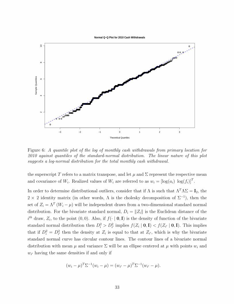
−3 −2 −1 0 1 2 3

24

68

10

Normal Q−Q Plot for 2010 Cash Withdrawals

Theoretical Quantiles

Sa

mp

le Q

ua

ntil

es

Figure 6: A quantile plot of the log of monthly cash withdrawals from primary location for2010 against quantiles of the standard-normal distribution. The linear nature of this plotsuggests a log-normal distribution for the total monthly cash withdrawal.

the superscript T refers to a matrix transpose, and let µ and Σ represent the respective mean

and covariance of Wi. Realized values of Wi are referred to as wi = [log(ai) log(fi)]T .

In order to determine distributional outliers, consider that if Λ is such that ΛTΛΣ = I2, the

2 × 2 identity matrix (in other words, Λ is the cholesky decomposition of Σ−1), then the

set of Zi = ΛT (Wi− µ) will be independent draws from a two-dimensional standard normal

distribution. For the bivariate standard normal, Di = ‖Zi‖ is the Euclidean distance of the

ith draw, Zi, to the point (0, 0). Also, if f(· | 0, I) is the density of function of the bivariate

standard normal distribution then D2i > D2

i′ implies f(Zi | 0, I) < f(Zi′ | 0, I). This implies

that if D2i = D2

i′ then the density at Zi is equal to that at Zi′ , which is why the bivariate

standard normal curve has circular contour lines. The contour lines of a bivariate normal

distribution with mean µ and variance Σ will be an ellipse centered at µ with points wi and

wi′ having the same densities if and only if

(wi − µ)TΣ−1(wi − µ) = (wi′ − µ)TΣ−1(wi′ − µ).

33

Transforming the N independent draws from the true distribution to N independent draws

of the bivariate distribution makes it easier to work with the data. This transformation

preserves the sense of distance from the mean given by the density (which is lower for less

likely points and decreases as one moves away from the mean). Therefore, if wi and wi′ are

such that d2i > d2i′ then f(wi | µ,Σ) < f(wi′ | µ,Σ). So, the extremity of each of the N points

can be measured by considering how likely it is to have come from the assumed distribution,

by comparing the observed r2i .

It is known that D2i are independent and identically distributed random variables from the

Exp(0.5) or equivalently a Chi-Square(2) distribution. Therefore, it is simple to apply the

theory of order statistics to them. Consider ordering the observed D2i , with D2

(i) representing

the ith largest observed value, and let G(·) be the cumulative distribution function of the

Exp(0.5) (or Chi-Square(2)) distribution. Standard distribution theory states that G(D2(i)) ∼

Beta(N − i+ 1, i).

Therefore, for the ith least likely observation, the Beta distribution defines a 95 percent

confidence interval for G(D2(i)) from which one can determine a corresponding 95 percent

confidence interval for D2(i) (because G(·) is monotonic). Other percentiles can also be cal-

culated; let Qi,p correspond to the pth percentile for D(i).

Within each iteration of the algorithm, µ and Σ are estimated by µ and Σ from the data via

the sample means, variances, and covariances of the raw data. Then, under the distributional

assumptions and under the null hypothesis that all data points are valid, it is possible to

estimate whether the least likely observation (that which has the largest d2i ) is consistent with

the theoretical distribution for D2(1). This is done by constructing a 95 percent confidence

interval for D2(1) and simply seeing whether the corresponding observed value falls in this

interval. If it does, it seems that the data, at least in the extremities, are consistent with

the initial assumption. If it does not, then the procedure reassigns the data entry to a

point consistent with the fitted distribution but a minimum distance from the original value.

Specifically, the data point is reassigned so that its new d2i value corresponds to the median

of the distribution of D2(1). If such an imputation is made, the entire process begins again

with the updated dataset. This continues until no more data points are identified.

Here, the imputation process is developed. For simplicity of notation, consider that k is such

that d2k = d2(1) in the observed data, and assume that this value is not consistent with the

theoretical expectation. zk is first reassigned to znewk and then converted from the standard

normal distribution to that of interest by letting

wnewk = µ+ Λ−T znewk .

34

Algorithm 2 Preprocessing: Monthly Cash Withdrawal

Let wi = (log(ai), log(fi)) for all i = 1, . . . , NSet done.algorithm = 0 {will be 1 only when no more outliers}Calculate q1,.025, q1,.5 and q1,.975 based on N iid observationswhile done.algorithm = 0 do

Estimate µ = mean(wi) and Σ = var(wi) from sample statistics of the wiCalculate Λ such that ΛT Λ = Σ−1

for i = 1, . . . , N doCalculate zi = ΛT (wi − µ)Calculate di = ‖zi‖2

end forFind k such that dk = d(1).if dk ≤ q1,.975 then

Set done.algorithm = 1end ifif dk > q1,.975 then

Calculate znewk

Calculate wnewk = µ+ Λ−T znewk

Replace wk with wnewk

end ifend whileKeep changes to wi only if log(ai) < µA and log(fi) < µF .

Then, the only element left to be determined is znewk . But this is relatively simple, as it

is a constrained optimization problem. Namely, if q1,.5 corresponds to the median of the

theoretical distribution of D(1), then znewk is such that ‖znewk − zk‖2 (the distance between

the old and new points) is minimized, subject to the condition ‖znewk ‖2 = q1,.5. Optimization

programs for this paradigm are well known and available for most computational packages

(Press et al. 2007)

The process is illustrated in Figure 7, which shows the first iteration of the cleaning algorithm

for the 2010 data. The plot shows the 95 percent confidence interval for the most extreme

observation on the original distribution rather than the standard normal distribution, as well

as the median. The identified extreme point is clearly outside the interval, so it is moved

inside in such a way as to be as close as possible to the original data point.

An important consideration with this procedure is that an extreme point on the logarithmic

scale could be one whose withdrawal level is simply very small (close to 0). For example, if a

person reports an amount of 1 and a frequency of 0.25, the value of w will be (0,−1.38), which

could be determined to be very unlikely given the much higher average values of frequency

and amount. As a basis of comparison, the mean of the logarithms generally tends to fall

35

●

●

●

●

●

●

●

●

●

●

●

● ●

●

●

●

●

●

●

●

●

●

●

●●

●

●

●

●

●

●

●

●

●●

●

●●

●

●

●

●

●

●

●

●

●

●

●

●

●

●

●

●

●

●

●

●

●

●

●

●●

●

●

●

●

●

●

●

●

●

●

●

●

●

●

●●

●

●

●

●

●

●

●

●

●

●

●

●

●

●

●

●

●

●

●

●

●

●

●

●

●

●

●

●

●

●

●

●

●

●

●

●

●

●

●●

●

●

●

●

●

●

●●

●

●

●

●

●

●●

●

●

●

●●

●

●

●

●

●

●

●●

●

●

●

●

●●

●●

●

●●

●

●

●

●

●

●

●●

●

●

●

●

●

●

●

●

●

●

●●●

●●

●

●

●

●

●

●

●

●

●

●

●●

● ●

●

●

●

●

●

●

●

●●

●

●

●●●

●

●

●

●

●●

●

●

●

●

●

●

●

●

●

●

●

●

●

●

●

●

●

●

●

●

●

●●

●

●

●

●

●

●

●

●

●

●

●

●

●

●

●

●

●

●

●

●●

●

●

●

● ●

●

●

●●

●

●

●

●

●

●

●

●

●

●

●●

●

●

●

●

●

●

●

●

●●

●

●

●

●

●

●

●●

●

●

●

●

●

●

●

●

●

●

●

●

●

●●

●

●

●

●

●

●

●●

●

●

●

●

●●

●

●

●

●

●

●

●

●

●

●

●

●

●

●

●

●

●

●

●

●

●

●

● ●

●

● ●

●

●

●

●

●

●

●

●

●

●

●

●

●

●

●

●

●

●

●

●

●

●

●

●●

●

●

●

●

●

●

●

●

●

●●

●●

●

●

●

●

●

●

●

●

●

●

●

●

●

●

●

●

●

●

●

●

●

●

●

●

●

●

●

●

●

●

●

●

● ●

●

●

●

●

●

●●

●

●

●

●

●

●

●

●

●●

●

●

●

●

●

●

●

●

●

●

●

●

●

●

●

●

●

●

●

●

●

●●

●

●

●●

● ●

●

●

●

●

●

●

●

●

●

●

●

●●

●

●

●

●

●●

●

●

●

●

●

●

●

● ●

●

●

●

●

●

●

●

●

●

●

●

●

●

●

●

● ●

●

●●

●●

●

●●

●

●

●

●

●

●

●●

●

●

●

●

●

●

●

●

●

●

●●

●

●●

●●

●

●●

●

●

●

●

●

●

●

●

● ●

●

●

●

● ●

●

●

●

●

● ●

●●

●

●

●

●

●●

●

●

●

●●

●

●

●

●

●

●

●

●

●

●

●

●

●

●

●

●

●

●

●

●

●

●

●

●

●

●

●

●

●

●

●

●

●●

●

●

●

●

●

●

●

●

●

●

●

● ●

●

●

●

●

● ●

●

●

●●

●

●

●

●

●

●

●

●

●●

●

●

●

●

●

●

●

●

●

●

●

●

●

●

●

●

●

● ●

●

●

●

●

●

●●

●

●

●

●

●

●

●●

●

●

●

●

●

●

●

●

●

●

●

●

●

●

●●

●

●

●

●

●

●

●

●

●

●

●

●

●

●

●

●

●●

●

●

●

●

●●

●

●

●

●

●●

●

●

●

●

●

●

●

●

●

●

●

●

●

●●

● ●

●

●

●

●● ●

●

●

●

●

●●

●

●

●

●

●

●

●

●

●

●

●

●

●

●

●

●●

●

●

●

●

●

●

●

●

●

●

●

●

●

●

●

●

●

●

●

●

●

●

●

●

●

●

●

●

●

●

●

●

●

●

●

●

●

●●

●

●

●

●

●

●

●

●

●

●

●

●

●

●

●

●

●

● ●

●

●

●

●

●

●

●●

●

●

●

●

●

●

●

●

●

●

●

●

●

●

●

●

●

●

●

●

●

●

●●

●

●

●

●

●

●

●

●

●●

●

●

●

●

●

●

●

●

●

●

●

●

●

●

●

●

●

●

●●

●

● ●●

●

●

●

●

●

●

●●

●

●

●

●

●

●

●

●

●

●

●

●

●

●

●●

●

●●

●

●

●

●

●●

●

●

●

●

●

●

●

●

●

●

●

●

●

●

●

●

●

●

●

●

●

●

●

●

●

●

●

●

●

●

●

●

●

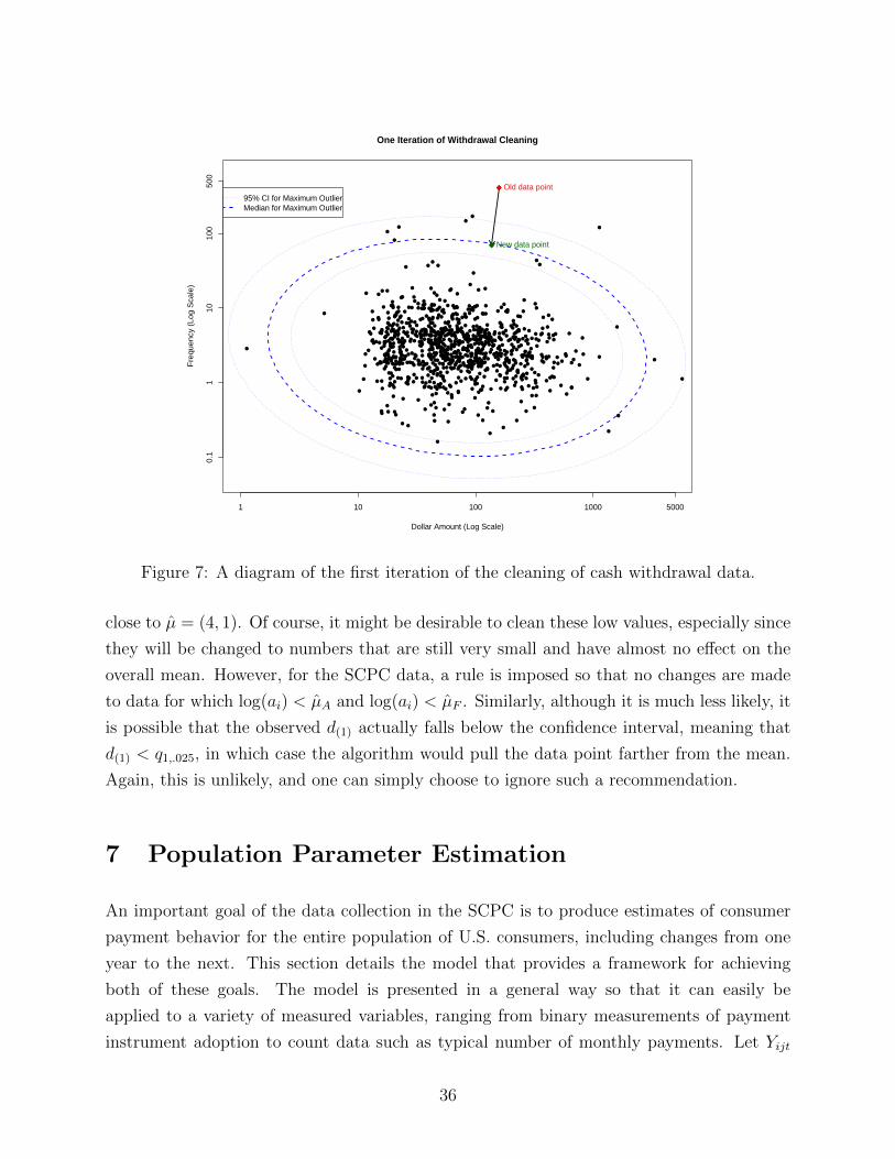
One Iteration of Withdrawal Cleaning

Dollar Amount (Log Scale)

Fre

quen

cy (

Log

Sca

le)

1 10 100 1000 5000

0.1

110

100

500

Old data point

New data point

95% CI for Maximum OutlierMedian for Maximum Outlier

Figure 7: A diagram of the first iteration of the cleaning of cash withdrawal data.

close to µ = (4, 1). Of course, it might be desirable to clean these low values, especially since

they will be changed to numbers that are still very small and have almost no effect on the

overall mean. However, for the SCPC data, a rule is imposed so that no changes are made

to data for which log(ai) < µA and log(ai) < µF . Similarly, although it is much less likely, it

is possible that the observed d(1) actually falls below the confidence interval, meaning that

d(1) < q1,.025, in which case the algorithm would pull the data point farther from the mean.

Again, this is unlikely, and one can simply choose to ignore such a recommendation.

7 Population Parameter Estimation

An important goal of the data collection in the SCPC is to produce estimates of consumer

payment behavior for the entire population of U.S. consumers, including changes from one

year to the next. This section details the model that provides a framework for achieving

both of these goals. The model is presented in a general way so that it can easily be

applied to a variety of measured variables, ranging from binary measurements of payment

instrument adoption to count data such as typical number of monthly payments. Let Yijt

36

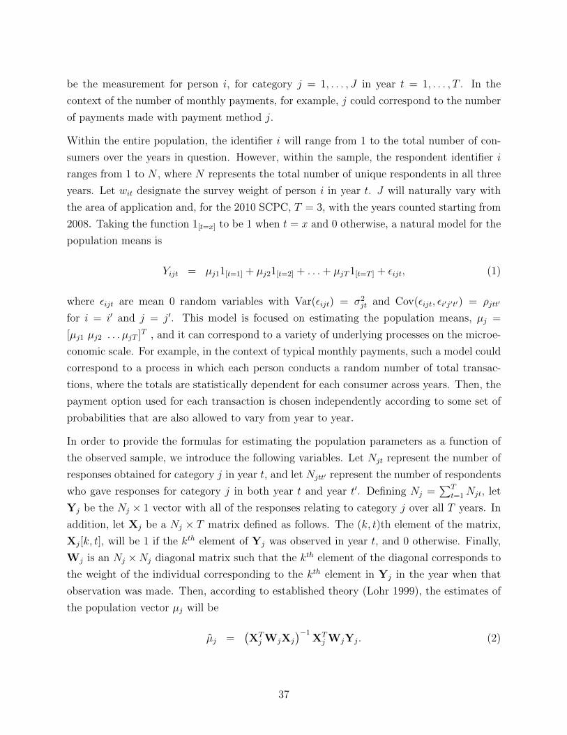
be the measurement for person i, for category j = 1, . . . , J in year t = 1, . . . , T . In the

context of the number of monthly payments, for example, j could correspond to the number

of payments made with payment method j.

Within the entire population, the identifier i will range from 1 to the total number of con-

sumers over the years in question. However, within the sample, the respondent identifier i

ranges from 1 to N , where N represents the total number of unique respondents in all three

years. Let wit designate the survey weight of person i in year t. J will naturally vary with

the area of application and, for the 2010 SCPC, T = 3, with the years counted starting from

2008. Taking the function 1[t=x] to be 1 when t = x and 0 otherwise, a natural model for the

population means is

Yijt = µj11[t=1] + µj21[t=2] + . . .+ µjT1[t=T ] + εijt, (1)

where εijt are mean 0 random variables with Var(εijt) = σ2jt and Cov(εijt, εi′j′t′) = ρjtt′

for i = i′ and j = j′. This model is focused on estimating the population means, µj =

[µj1 µj2 . . . µjT ]T , and it can correspond to a variety of underlying processes on the microe-

conomic scale. For example, in the context of typical monthly payments, such a model could

correspond to a process in which each person conducts a random number of total transac-

tions, where the totals are statistically dependent for each consumer across years. Then, the

payment option used for each transaction is chosen independently according to some set of

probabilities that are also allowed to vary from year to year.

In order to provide the formulas for estimating the population parameters as a function of

the observed sample, we introduce the following variables. Let Njt represent the number of

responses obtained for category j in year t, and let Njtt′ represent the number of respondents

who gave responses for category j in both year t and year t′. Defining Nj =∑T

t=1Njt, let

Yj be the Nj × 1 vector with all of the responses relating to category j over all T years. In

addition, let Xj be a Nj × T matrix defined as follows. The (k, t)th element of the matrix,

Xj[k, t], will be 1 if the kth element of Yj was observed in year t, and 0 otherwise. Finally,

Wj is an Nj ×Nj diagonal matrix such that the kth element of the diagonal corresponds to

the weight of the individual corresponding to the kth element in Yj in the year when that

observation was made. Then, according to established theory (Lohr 1999), the estimates of

the population vector µj will be

µj =(XTj WjXj

)−1XTj WjYj. (2)

37

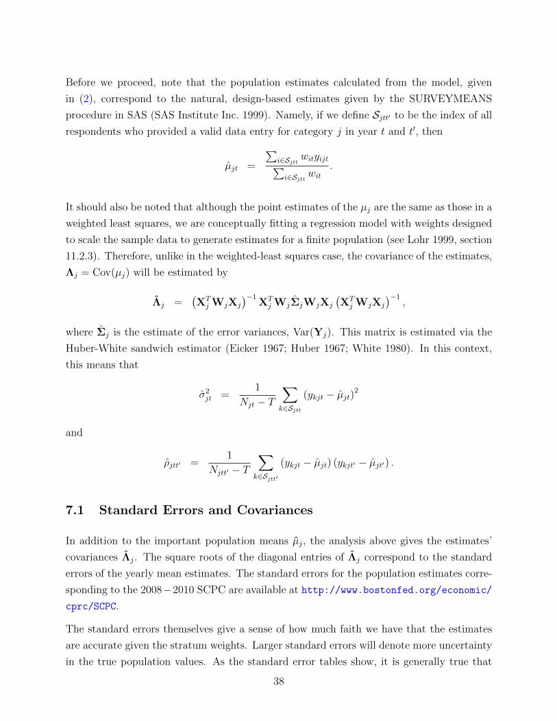
Before we proceed, note that the population estimates calculated from the model, given

in (2), correspond to the natural, design-based estimates given by the SURVEYMEANS

procedure in SAS (SAS Institute Inc. 1999). Namely, if we define Sjtt′ to be the index of all

respondents who provided a valid data entry for category j in year t and t′, then

µjt =

∑i∈Sjtt wityijt∑i∈Sjtt wit

.

It should also be noted that although the point estimates of the µj are the same as those in a

weighted least squares, we are conceptually fitting a regression model with weights designed

to scale the sample data to generate estimates for a finite population (see Lohr 1999, section

11.2.3). Therefore, unlike in the weighted-least squares case, the covariance of the estimates,

Λj = Cov(µj) will be estimated by

Λj =(XTj WjXj

)−1XTj WjΣjWjXj

(XTj WjXj

)−1,

where Σj is the estimate of the error variances, Var(Yj). This matrix is estimated via the

Huber-White sandwich estimator (Eicker 1967; Huber 1967; White 1980). In this context,

this means that

σ2jt =

1

Njt − T∑k∈Sjtt

(ykjt − µjt)2

and

ρjtt′ =1

Njtt′ − T∑k∈Sjtt′

(ykjt − µjt) (ykjt′ − µjt′) .

7.1 Standard Errors and Covariances

In addition to the important population means µj, the analysis above gives the estimates’

covariances Λj. The square roots of the diagonal entries of Λj correspond to the standard

errors of the yearly mean estimates. The standard errors for the population estimates corre-

sponding to the 2008−2010 SCPC are available at http://www.bostonfed.org/economic/

cprc/SCPC.

The standard errors themselves give a sense of how much faith we have that the estimates

are accurate given the stratum weights. Larger standard errors will denote more uncertainty

in the true population values. As the standard error tables show, it is generally true that

38

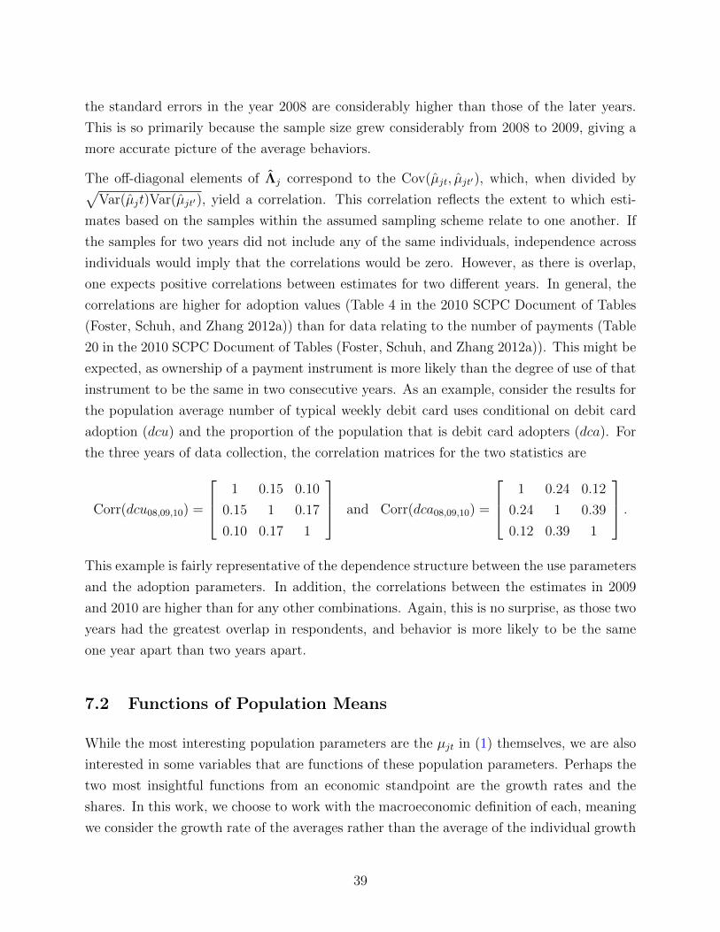
the standard errors in the year 2008 are considerably higher than those of the later years.

This is so primarily because the sample size grew considerably from 2008 to 2009, giving a

more accurate picture of the average behaviors.

The off-diagonal elements of Λj correspond to the Cov(µjt, µjt′), which, when divided by√Var(µjt)Var(µjt′), yield a correlation. This correlation reflects the extent to which esti-

mates based on the samples within the assumed sampling scheme relate to one another. If

the samples for two years did not include any of the same individuals, independence across

individuals would imply that the correlations would be zero. However, as there is overlap,

one expects positive correlations between estimates for two different years. In general, the

correlations are higher for adoption values (Table 4 in the 2010 SCPC Document of Tables

(Foster, Schuh, and Zhang 2012a)) than for data relating to the number of payments (Table

20 in the 2010 SCPC Document of Tables (Foster, Schuh, and Zhang 2012a)). This might be

expected, as ownership of a payment instrument is more likely than the degree of use of that

instrument to be the same in two consecutive years. As an example, consider the results for

the population average number of typical weekly debit card uses conditional on debit card

adoption (dcu) and the proportion of the population that is debit card adopters (dca). For

the three years of data collection, the correlation matrices for the two statistics are

Corr(dcu08,09,10) =

1 0.15 0.10

0.15 1 0.17

0.10 0.17 1

and Corr(dca08,09,10) =

1 0.24 0.12

0.24 1 0.39

0.12 0.39 1

.This example is fairly representative of the dependence structure between the use parameters

and the adoption parameters. In addition, the correlations between the estimates in 2009

and 2010 are higher than for any other combinations. Again, this is no surprise, as those two

years had the greatest overlap in respondents, and behavior is more likely to be the same

one year apart than two years apart.

7.2 Functions of Population Means

While the most interesting population parameters are the µjt in (1) themselves, we are also

interested in some variables that are functions of these population parameters. Perhaps the

two most insightful functions from an economic standpoint are the growth rates and the

shares. In this work, we choose to work with the macroeconomic definition of each, meaning

we consider the growth rate of the averages rather than the average of the individual growth

39

rates. We thus let

gjt =µj,t+1 − µjt

µjt(3)

be the growth rate of category j from year t to t+ 1, and

sjt =µjt∑Jk=1 µkt

(4)

be the share of category j in year t.

The macroeconomic definitions used in (3) and (4) should be contrasted with their micro-

economic alternatives. The former involve defining individual shares for each category,

s ijt =yijt∑J

k=1 yiktand estimating sjt by applying (1) and (2) to this individual variable. The

macroeconomic approach is statistically sounder, as, under most models that treat individ-

uals as independent, it will give the maximum likelihood estimates of the parameters in

question. For example, if the total number of payments for person i at time t is Yit modeled

as a Poisson random variable and the number assigned to category j, Yijt is a binomial

distribution conditional on Yit with probability pjt, then the maximum likelihood estimates

for the pjt will be given by∑

i Yijt∑i Yit

rather than∑

iYijtNYit

(in this example, we have made all

weights equal to simplify the equations). Thus, throughout this analysis, we generally use

the macroeconomic definitions.

7.2.1 Generating U.S. Aggregate Estimates

The term µjt in (1) represents a population mean in year t. For example, if the variable of

interest is the number of payments made in a typical month with cash, then µjt represents the

average of this value with respect to all U.S. adult consumers. In theory, if µjt is an estimate

of this mean, then a corresponding estimate for the aggregate number among the entire

population would be µjt multiplied by the size of the population. However, such calculations

must be taken with caution. The estimates of µjt from the SCPC are likely to be fairly

variable due to the relatively small sample size and variation in the post-stratification weights.

Thus, while the estimates might be unbiased, any one estimate based on a particular sample

is potentially a relatively poor estimate of µjt. Any difference between µjt and µjt is magnified

when multiplied by the U.S. population, making the resulting estimate a potentially poor

estimate of the population aggregate. The high degree of error in these aggregate estimates

is the reason we recommend that such methodologies be taken with caution. Issues of bias in

the estimates could arise as a result of the sampling instrument and potential measurement

40

errors. For example, the SCPC asks respondents for their personal rather than household

payment choices. Inability to clearly delineate all payments related to the household, such

as bills, could lead to systematically inaccurate responses.

8 Hypothesis Tests for Temporal Changes in Consumer

Payments

Knowledge of µj and Λj for all j = 1, . . . , J also allows one to make inferences and test

hypotheses about the population across the different years. In the following subsections, we

delineate and conduct a variety of hypothesis tests with the general goal of assessing changes

from 2009 to 2010 in the payment behavior of consumers. The tests are done primarily for

the data on the number of monthly payments for various payment methods and transaction

types. The population estimates for all years are shown in Tables 20 and 21 in the 2010

SCPC Document of Tables (Foster, Schuh, and Zhang 2012a).

8.1 Hypothesis Tests for Means

Perhaps the most basic assertion one would like to make is the degree to which the population

means change over time. Therefore, in the context of the model outlined above, we consider

the following hypotheses:

Ho : µjt = µjt′ Ha : µjt 6= µjt′ .

In order to do so, we need to estimate Var(µjt′−µjt), which we do by estimating the identity:

Var(µjt′ − µjt) = Var(µjt′) + Var(µjt)− 2Cov(µjt′ , µjt)

with

Var(µjt′ − µjt) = Λj[t′, t′] + Λj[t, t]− 2Λj[t, t

′].

Now, under the null hypothesis, the test statistic

Z =µjt′ − µjt√

Var(µjt′ − µjt)

41

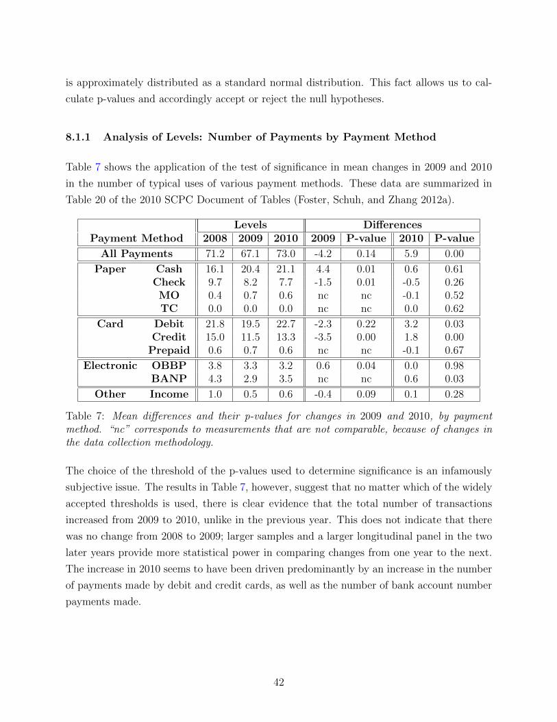
is approximately distributed as a standard normal distribution. This fact allows us to cal-

culate p-values and accordingly accept or reject the null hypotheses.

8.1.1 Analysis of Levels: Number of Payments by Payment Method

Table 7 shows the application of the test of significance in mean changes in 2009 and 2010

in the number of typical uses of various payment methods. These data are summarized in

Table 20 of the 2010 SCPC Document of Tables (Foster, Schuh, and Zhang 2012a).

Levels DifferencesPayment Method 2008 2009 2010 2009 P-value 2010 P-value

All Payments 71.2 67.1 73.0 -4.2 0.14 5.9 0.00

Paper Cash 16.1 20.4 21.1 4.4 0.01 0.6 0.61Check 9.7 8.2 7.7 -1.5 0.01 -0.5 0.26MO 0.4 0.7 0.6 nc nc -0.1 0.52TC 0.0 0.0 0.0 nc nc 0.0 0.62

Card Debit 21.8 19.5 22.7 -2.3 0.22 3.2 0.03Credit 15.0 11.5 13.3 -3.5 0.00 1.8 0.00

Prepaid 0.6 0.7 0.6 nc nc -0.1 0.67

Electronic OBBP 3.8 3.3 3.2 0.6 0.04 0.0 0.98BANP 4.3 2.9 3.5 nc nc 0.6 0.03

Other Income 1.0 0.5 0.6 -0.4 0.09 0.1 0.28

Table 7: Mean differences and their p-values for changes in 2009 and 2010, by paymentmethod. “nc” corresponds to measurements that are not comparable, because of changes inthe data collection methodology.

The choice of the threshold of the p-values used to determine significance is an infamously

subjective issue. The results in Table 7, however, suggest that no matter which of the widely

accepted thresholds is used, there is clear evidence that the total number of transactions

increased from 2009 to 2010, unlike in the previous year. This does not indicate that there

was no change from 2008 to 2009; larger samples and a larger longitudinal panel in the two

later years provide more statistical power in comparing changes from one year to the next.

The increase in 2010 seems to have been driven predominantly by an increase in the number

of payments made by debit and credit cards, as well as the number of bank account number

payments made.

42

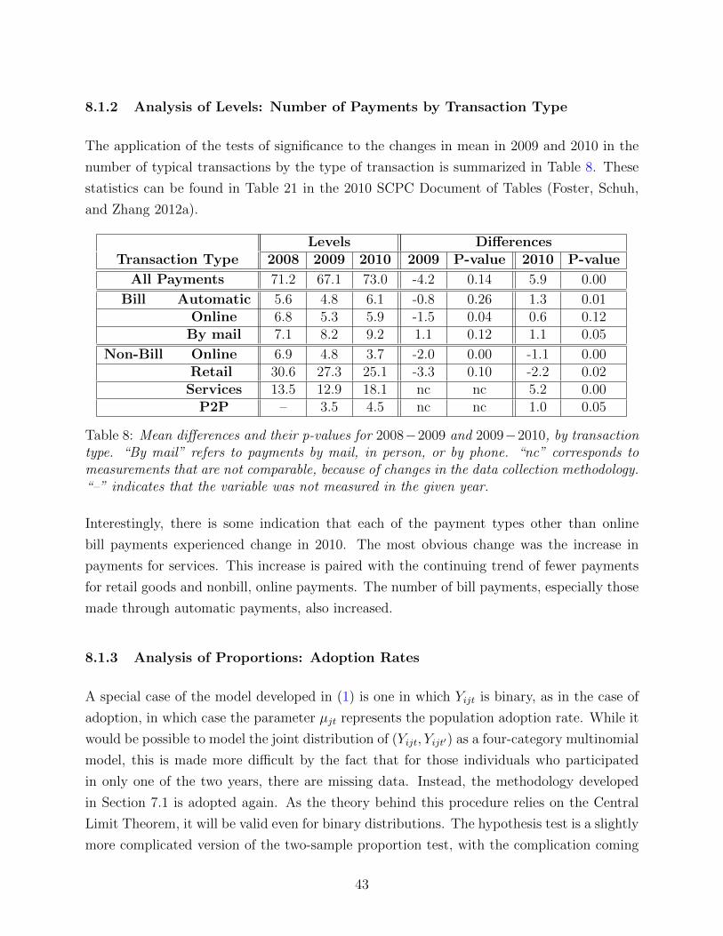
8.1.2 Analysis of Levels: Number of Payments by Transaction Type

The application of the tests of significance to the changes in mean in 2009 and 2010 in the

number of typical transactions by the type of transaction is summarized in Table 8. These

statistics can be found in Table 21 in the 2010 SCPC Document of Tables (Foster, Schuh,

and Zhang 2012a).

Levels DifferencesTransaction Type 2008 2009 2010 2009 P-value 2010 P-value

All Payments 71.2 67.1 73.0 -4.2 0.14 5.9 0.00

Bill Automatic 5.6 4.8 6.1 -0.8 0.26 1.3 0.01Online 6.8 5.3 5.9 -1.5 0.04 0.6 0.12

By mail 7.1 8.2 9.2 1.1 0.12 1.1 0.05

Non-Bill Online 6.9 4.8 3.7 -2.0 0.00 -1.1 0.00Retail 30.6 27.3 25.1 -3.3 0.10 -2.2 0.02Services 13.5 12.9 18.1 nc nc 5.2 0.00

P2P – 3.5 4.5 nc nc 1.0 0.05

Table 8: Mean differences and their p-values for 2008−2009 and 2009−2010, by transactiontype. “By mail” refers to payments by mail, in person, or by phone. “nc” corresponds tomeasurements that are not comparable, because of changes in the data collection methodology.“–” indicates that the variable was not measured in the given year.

Interestingly, there is some indication that each of the payment types other than online

bill payments experienced change in 2010. The most obvious change was the increase in

payments for services. This increase is paired with the continuing trend of fewer payments

for retail goods and nonbill, online payments. The number of bill payments, especially those

made through automatic payments, also increased.

8.1.3 Analysis of Proportions: Adoption Rates

A special case of the model developed in (1) is one in which Yijt is binary, as in the case of

adoption, in which case the parameter µjt represents the population adoption rate. While it

would be possible to model the joint distribution of (Yijt, Yijt′) as a four-category multinomial

model, this is made more difficult by the fact that for those individuals who participated

in only one of the two years, there are missing data. Instead, the methodology developed

in Section 7.1 is adopted again. As the theory behind this procedure relies on the Central

Limit Theorem, it will be valid even for binary distributions. The hypothesis test is a slightly

more complicated version of the two-sample proportion test, with the complication coming

43

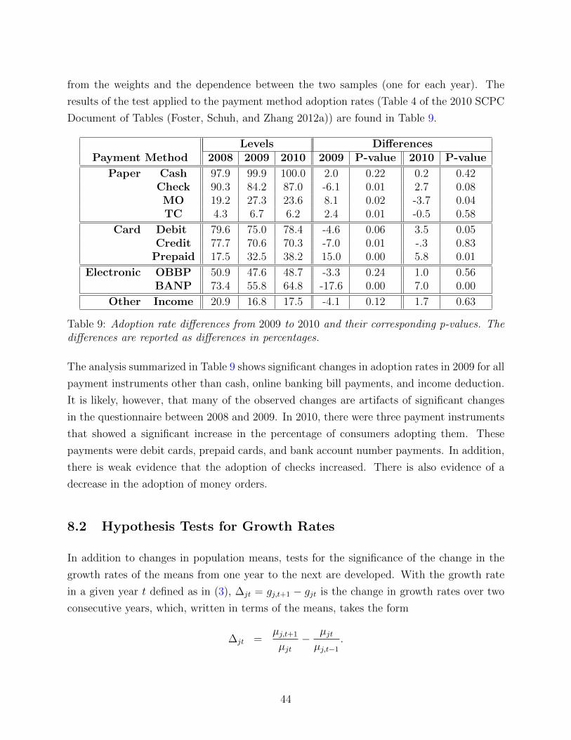
from the weights and the dependence between the two samples (one for each year). The

results of the test applied to the payment method adoption rates (Table 4 of the 2010 SCPC

Document of Tables (Foster, Schuh, and Zhang 2012a)) are found in Table 9.

Levels DifferencesPayment Method 2008 2009 2010 2009 P-value 2010 P-value

Paper Cash 97.9 99.9 100.0 2.0 0.22 0.2 0.42Check 90.3 84.2 87.0 -6.1 0.01 2.7 0.08MO 19.2 27.3 23.6 8.1 0.02 -3.7 0.04TC 4.3 6.7 6.2 2.4 0.01 -0.5 0.58

Card Debit 79.6 75.0 78.4 -4.6 0.06 3.5 0.05Credit 77.7 70.6 70.3 -7.0 0.01 -.3 0.83

Prepaid 17.5 32.5 38.2 15.0 0.00 5.8 0.01

Electronic OBBP 50.9 47.6 48.7 -3.3 0.24 1.0 0.56BANP 73.4 55.8 64.8 -17.6 0.00 7.0 0.00

Other Income 20.9 16.8 17.5 -4.1 0.12 1.7 0.63

Table 9: Adoption rate differences from 2009 to 2010 and their corresponding p-values. Thedifferences are reported as differences in percentages.

The analysis summarized in Table 9 shows significant changes in adoption rates in 2009 for all

payment instruments other than cash, online banking bill payments, and income deduction.

It is likely, however, that many of the observed changes are artifacts of significant changes

in the questionnaire between 2008 and 2009. In 2010, there were three payment instruments

that showed a significant increase in the percentage of consumers adopting them. These

payments were debit cards, prepaid cards, and bank account number payments. In addition,

there is weak evidence that the adoption of checks increased. There is also evidence of a

decrease in the adoption of money orders.

8.2 Hypothesis Tests for Growth Rates

In addition to changes in population means, tests for the significance of the change in the

growth rates of the means from one year to the next are developed. With the growth rate

in a given year t defined as in (3), ∆jt = gj,t+1 − gjt is the change in growth rates over two

consecutive years, which, written in terms of the means, takes the form

∆jt =µj,t+1

µjt− µjtµj,t−1

.

44

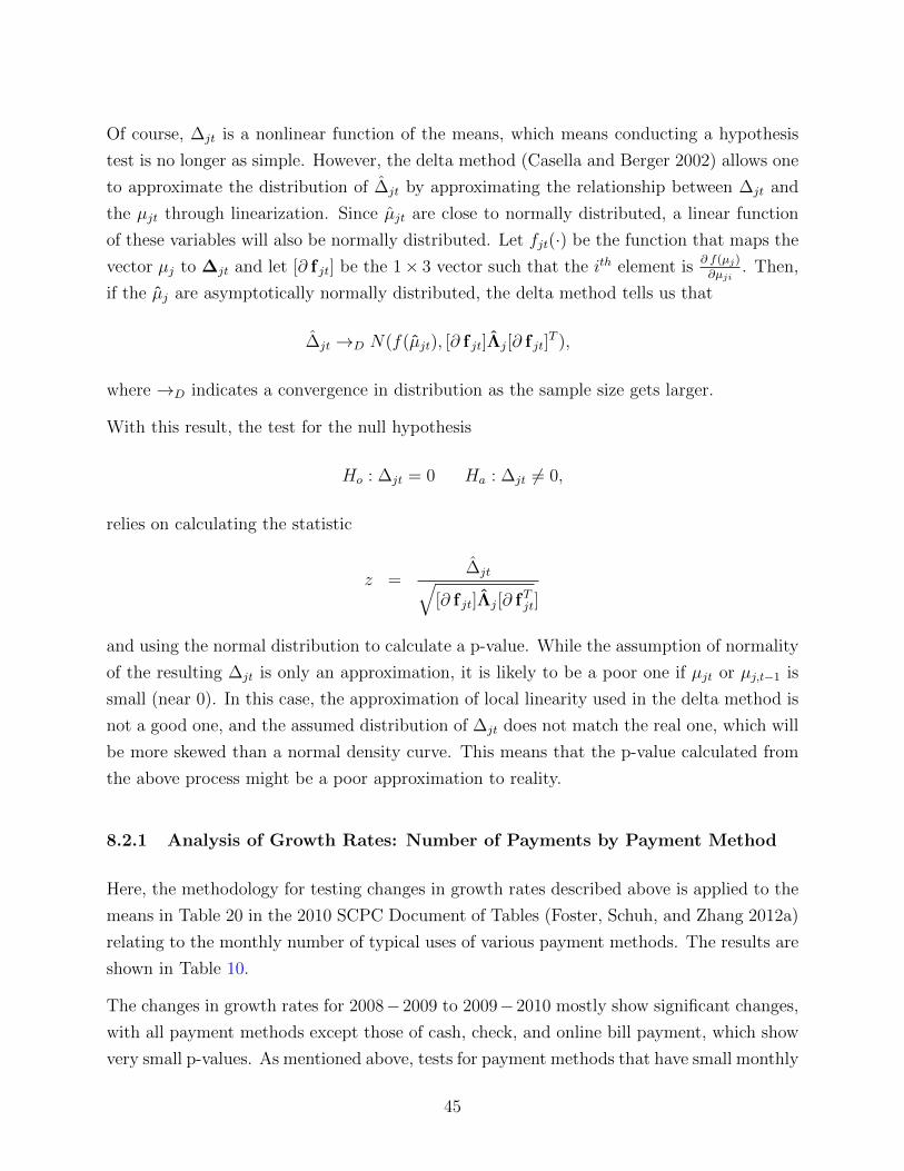
Of course, ∆jt is a nonlinear function of the means, which means conducting a hypothesis

test is no longer as simple. However, the delta method (Casella and Berger 2002) allows one

to approximate the distribution of ∆jt by approximating the relationship between ∆jt and

the µjt through linearization. Since µjt are close to normally distributed, a linear function

of these variables will also be normally distributed. Let fjt(·) be the function that maps the

vector µj to ∆jt and let [∂ f jt] be the 1× 3 vector such that the ith element is∂ f(µj)

∂µji. Then,

if the µj are asymptotically normally distributed, the delta method tells us that

∆jt →D N(f(µjt), [∂ f jt]Λj[∂ f jt]T ),

where →D indicates a convergence in distribution as the sample size gets larger.

With this result, the test for the null hypothesis

Ho : ∆jt = 0 Ha : ∆jt 6= 0,

relies on calculating the statistic

z =∆jt√

[∂ f jt]Λj[∂ fTjt]

and using the normal distribution to calculate a p-value. While the assumption of normality

of the resulting ∆jt is only an approximation, it is likely to be a poor one if µjt or µj,t−1 is

small (near 0). In this case, the approximation of local linearity used in the delta method is

not a good one, and the assumed distribution of ∆jt does not match the real one, which will

be more skewed than a normal density curve. This means that the p-value calculated from

the above process might be a poor approximation to reality.

8.2.1 Analysis of Growth Rates: Number of Payments by Payment Method

Here, the methodology for testing changes in growth rates described above is applied to the

means in Table 20 in the 2010 SCPC Document of Tables (Foster, Schuh, and Zhang 2012a)

relating to the monthly number of typical uses of various payment methods. The results are

shown in Table 10.

The changes in growth rates for 2008−2009 to 2009−2010 mostly show significant changes,

with all payment methods except those of cash, check, and online bill payment, which show

very small p-values. As mentioned above, tests for payment methods that have small monthly

45

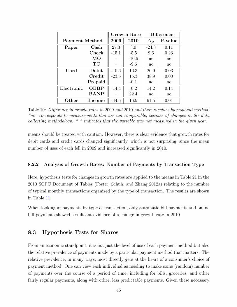
Growth Rate Difference

Payment Method 2009 2010 ∆jt P-value

Paper Cash 27.3 3.0 -24.3 0.11Check -15.1 -5.5 9.6 0.23MO – -10.6 nc ncTC – -9.6 nc nc

Card Debit -10.6 16.3 26.9 0.03Credit -23.5 15.3 38.9 0.00

Prepaid – -0.1 nc nc

Electronic OBBP -14.4 -0.2 14.2 0.14BANP – 22.4 nc nc

Other Income -44.6 16.9 61.5 0.01

Table 10: Difference in growth rates in 2009 and 2010 and their p-values by payment method.“nc” corresponds to measurements that are not comparable, because of changes in the datacollecting methodology. “–” indicates that the variable was not measured in the given year.

means should be treated with caution. However, there is clear evidence that growth rates for

debit cards and credit cards changed significantly, which is not surprising, since the mean

number of uses of each fell in 2009 and increased significantly in 2010.

8.2.2 Analysis of Growth Rates: Number of Payments by Transaction Type

Here, hypothesis tests for changes in growth rates are applied to the means in Table 21 in the

2010 SCPC Document of Tables (Foster, Schuh, and Zhang 2012a) relating to the number

of typical monthly transactions organized by the type of transaction. The results are shown

in Table 11.

When looking at payments by type of transaction, only automatic bill payments and online

bill payments showed significant evidence of a change in growth rate in 2010.

8.3 Hypothesis Tests for Shares

From an economic standpoint, it is not just the level of use of each payment method but also

the relative prevalence of payments made by a particular payment method that matters. The

relative prevalence, in many ways, most directly gets at the heart of a consumer’s choice of

payment method. One can view each individual as needing to make some (random) number

of payments over the course of a period of time, including for bills, groceries, and other

fairly regular payments, along with other, less predictable payments. Given these necessary

46

Growth Rate Difference

Transaction Type 2009 2010 ∆jt P-value

Bill Automatic -26.9 25.9 52.7 0.00Online -22.5 11.5 34.1 0.01

By mail 15.2 13.3 -1.9 0.90

Non-Bill Online -29.6 -23.3 6.4 0.52Retail -10.7 -8.2 2.5 0.74

Services – 40.2 nc ncP2P – 27.8 nc nc

Table 11: Difference in growth rates from 2008 − 2009 and 2009 − 2010 and their p-valuesby payment method. “By mail” refers to payments by mail, in person, or by phone.“nc” cor-responds to measurements that are not comparable, because of changes in the data collectingmethodology. “–” indicates that the variable was not measured in the given year.

payments, it is up to the consumer to decide how to execute each transaction. The decision

reflects a variety of factors such as convenience, cost, and acceptance of the payment method,

which is why the prevalence of payments is important to economists. The level of use or

growth rate will not reflect these aspects of the decision, since a decrease of use in terms

of frequency per month could actually correspond to an increase in prevalence if the total

number of payments decreased.

There are two statistics that can be used to measure prevalence. The first statistic is the

relative growth differential (RGD), which measures the difference between the growth rate

in the use of a particular payment option and the overall growth rate in the total number of

payments. After some simple algebra, the RGD for payment option j from year t to t′ is

Gjtt′ =µjt′

µjt−∑J

k=1 µkt′∑Jk=1 µkt

. (5)

The second commonly used statistic is the share differential (SD), defined to be the difference

in the percentage of all payments made by payment option j in two years. The mathematical

form is

Sjtt′ =µjt′∑Jk=1 µkt′

− µjt∑Jk=1 µkt

. (6)

In each case, the statistics of interest are nonlinear functions of the µjt and are evidently

dependent, making hypothesis testing more complicated. Again, the delta method is used,

although now it involves a joint, multi-variable hypothesis test. As mentioned above, normal

approximations to growth rates can be poor when the means are close to 0. The share

47

differential will not have this problem in this scenario, because the denominator, as the

mean number of monthly payments, will be large, making the linear approximation inherent

in the delta method a good one. For this reason, share differential is adopted as a preferred

measure of relative prevalence.

Below, the methodology for the multivariate delta method hypothesis test (Casella and

Berger 2002), as applied to the share differentials, is explained. For simplicity of notation,

let Sj stand for Sjtt′ in the following paragraphs. The necessity of a multivariate test is

due to the clear dependence between Sj and Sj′ . In fact, SJ = −∑J−1

j=1 Sj. This issue of

dependence means that the joint hypothesis test takes the form

Ho : S1 = S2 = . . . = SJ−1 = 0 Ha : Sj 6= 0 for at least one j.

Now, let S =[S1 S2 . . . SJ

]T, and let h(µt, µt′) be the function that maps the population

means to the share differential statistics with [∂h(µt, µt′)], the matrix of partial derivatives∂h(µt,µt′ )∂µj,k

for k = t, t′ and j = 1, . . . , J . Now, letting Λtt′ be the data estimate of the covariance

of [µ1t . . . µJt µ1t′ . . . µJt′ ]T , the multivariate version of the delta method tells us that

S →D N(h(µt, µt′), [∂h(µt, µt′)]Λtt′ [∂h(µt, µt′)]

−1).

For simplicity of notation, let

Ctt′ = [∂h(µt, µt′)]Λtt′ [∂h(µt, µt′)]T .

The matrix Ctt′ estimates the variances and covariances of the sample statistics Sjtt′ for

j = 1, . . . , J . Given this approximate multivariate normal distribution of dimension J , it is

known that under the null hypothesis, the statistic

Z = STtt′C−1tt′ Stt′

will be approximately Chi-square distributed with J-1 degrees of freedom. Therefore, Z ∼χ2J−1, a fact that can be used to calculate a p-value corresponding to the hypothesis.

Of course, such a test provides insight only into whether the collection of share differentials

is significantly different from the vector 0, but it is impossible to attribute the cause of

the rejection to any particular payment method. However, one can consider whether the

exclusion of any choice would make the relative share differentials of the remaining J − 1

choices consistent with the null hypothesis. Determining the joint 95 percent confidence

48

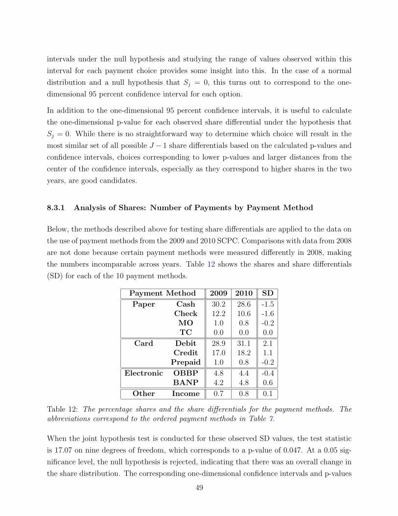
intervals under the null hypothesis and studying the range of values observed within this

interval for each payment choice provides some insight into this. In the case of a normal

distribution and a null hypothesis that Sj = 0, this turns out to correspond to the one-

dimensional 95 percent confidence interval for each option.

In addition to the one-dimensional 95 percent confidence intervals, it is useful to calculate

the one-dimensional p-value for each observed share differential under the hypothesis that

Sj = 0. While there is no straightforward way to determine which choice will result in the

most similar set of all possible J − 1 share differentials based on the calculated p-values and

confidence intervals, choices corresponding to lower p-values and larger distances from the

center of the confidence intervals, especially as they correspond to higher shares in the two

years, are good candidates.

8.3.1 Analysis of Shares: Number of Payments by Payment Method

Below, the methods described above for testing share differentials are applied to the data on

the use of payment methods from the 2009 and 2010 SCPC. Comparisons with data from 2008

are not done because certain payment methods were measured differently in 2008, making

the numbers incomparable across years. Table 12 shows the shares and share differentials

(SD) for each of the 10 payment methods.

Payment Method 2009 2010 SD

Paper Cash 30.2 28.6 -1.5Check 12.2 10.6 -1.6MO 1.0 0.8 -0.2TC 0.0 0.0 0.0

Card Debit 28.9 31.1 2.1Credit 17.0 18.2 1.1

Prepaid 1.0 0.8 -0.2

Electronic OBBP 4.8 4.4 -0.4BANP 4.2 4.8 0.6

Other Income 0.7 0.8 0.1

Table 12: The percentage shares and the share differentials for the payment methods. Theabbreviations correspond to the ordered payment methods in Table 7.

When the joint hypothesis test is conducted for these observed SD values, the test statistic

is 17.07 on nine degrees of freedom, which corresponds to a p-value of 0.047. At a 0.05 sig-

nificance level, the null hypothesis is rejected, indicating that there was an overall change in

the share distribution. The corresponding one-dimensional confidence intervals and p-values

49

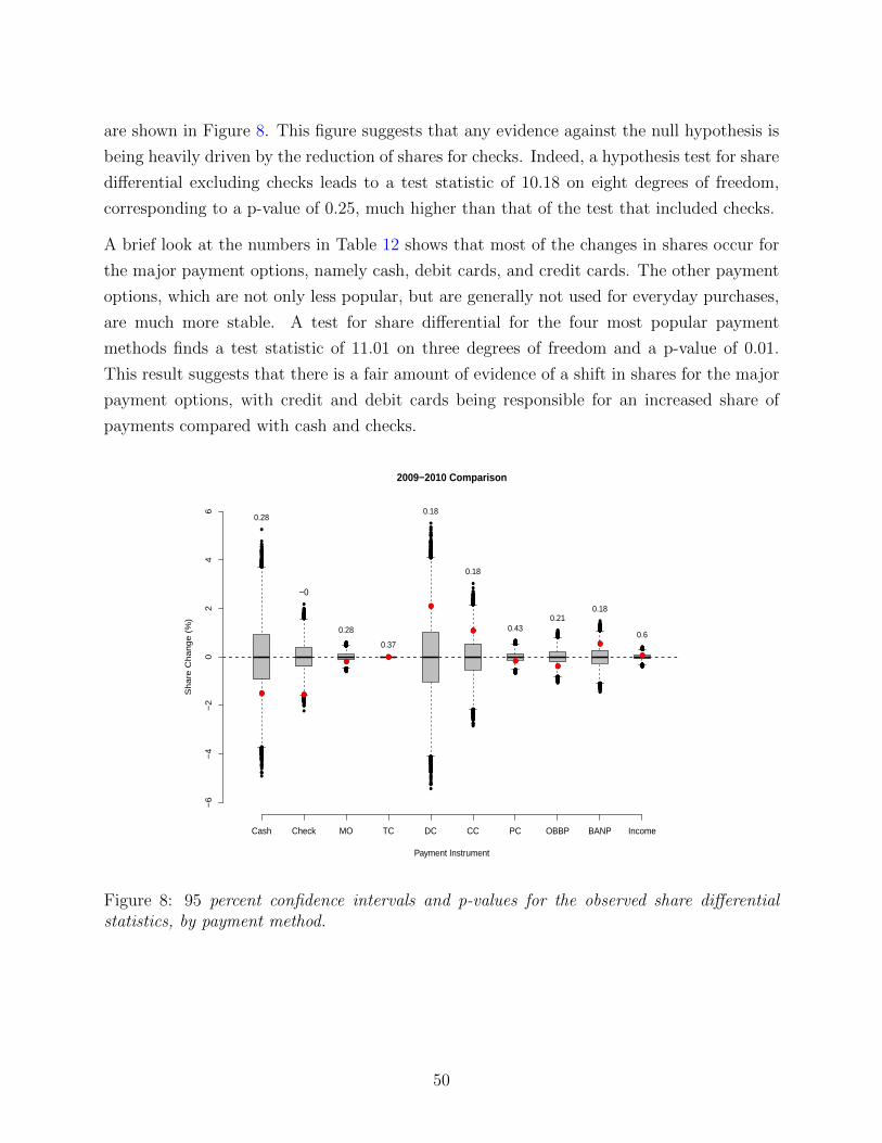
are shown in Figure 8. This figure suggests that any evidence against the null hypothesis is

being heavily driven by the reduction of shares for checks. Indeed, a hypothesis test for share

differential excluding checks leads to a test statistic of 10.18 on eight degrees of freedom,

corresponding to a p-value of 0.25, much higher than that of the test that included checks.

A brief look at the numbers in Table 12 shows that most of the changes in shares occur for

the major payment options, namely cash, debit cards, and credit cards. The other payment

options, which are not only less popular, but are generally not used for everyday purchases,

are much more stable. A test for share differential for the four most popular payment

methods finds a test statistic of 11.01 on three degrees of freedom and a p-value of 0.01.

This result suggests that there is a fair amount of evidence of a shift in shares for the major

payment options, with credit and debit cards being responsible for an increased share of

payments compared with cash and checks.

● ●

●●

●

●

●●

●

●

2009−2010 Comparison

Payment Instrument

Sh

are

Ch

an

ge

(%

)

Cash Check MO TC DC CC PC OBBP BANP Income

−6

−4

−2

02

46

●

●

●●●●

●

●

●

●

●

●

●

●

●

●

●

●

●

●

●

●

●

●

●

●

●

●

●

●

●

●

●●

●

●

●

●

●

●

●

●

●

●

●

●

●●●

●

●●

●●

●

●

●

●

●

●●

●●

●

●

●

●

●●

●

●●

●

●

●

●

●

●

●

●

●

●

●

●

●

●

●

●

●

●

●

●

●

●

●

●

●●

●

●

●●●

●

●

●

●

●●

●

●

●

●

●

●

●●

●

●●

●

●

●

●

●

●

●

●

●

●●

●

●

●●

●

●●

●

●●

●

●

●

●

●

●

●

●

●

●

●●

●

●

●

●

●

●

●

●

●

●●

●

●

●

●●

●

●

●

●●

●●

●

●●●●●

●●

●

●

●

●

●

●●

●

●

●

●

●

●●●●

●

●

●

●

●

●●

●●

●

●●●

●

●

●

●

●

●

●

●

●

●

●●●

●

●

●

●●

●

●●

●

●

●

●

●

●

●

●

●

●●

●

●●●●●

●

●

●

●

●

●

●

●●

●●

●

●

●

●●●

●●

●

●

●

●

●

●●

●●

●

●

●

●

●

●

●

●

●

●●●

●

●●

●

●●

●●

●

●●●●●●●

●

●

●

●

●

●

●

●●●

●

●

●

●

●

●

●

●

●●●

●

●●

●●

●

●

●●

●

●

●●

●

●

●

●●

●

●

●●●

●

●●

●

●

●

●

●

●

●

●

●

●

●

●●●

●●

●

●●●

●

●●

●●●

●●●

●●●

●●●

●●

●

●

●

●

●●

●●

●

●

●

●

●●●●

●●

●●

●●

●

●

●

●●

●

●●●●●●

●●●

●●

●●●●

●

●●

●

●

●●●

●

●●●

●

●

●

●●●

●

●

●

●

●

●

●

●

●

●

●

●

●●●●●

●●

●●●●

●●●●

●●

●●●●

●●

●

●●

●

●●●●●●●●●

●

●

●●

●

●●

●

●●

●

●●

●

●

●●●●

●

●

●

●

●

●

●

●●●●●

●

●●●●●

●●●

●

●●●●●●

●●●●

●●

●

●

●

●

●

●

●

●●

●

●

●●

●

●

●●

●●

●●●●●

●

●●●●●●

●

●●●●●●

●

●●

●●

●●●

●●

●●●●●●●●●

●●●

●●●●

●

●●●

●

●

●●●

●●

●●

●

●●●●

●●●

●●

●

●

●●

●●

●●

●

●

●●

●

●●●

●●

●●

●

●●●

●●●●

●●

●●

●

●

●●●

●

●

●●●●

●●●●

●

●●●●●●

●●●●

●

●

●●●

●●●

●●●●●

●●●

●●

●

●●

●

●

●●

●●●

●●●

●●●●●●●●●●●●●●●●●●●●●●●●●●●●●●●●●●●●●●●●●●●●●●●●●●●●●●●●●●●●●●●●●●●●●●●●●●●●●●●●●●●●●●●●●●●●●●●●●●●●●●●●●●●●●●●●●●●●●●●●●●●●●●●●●●●●●●●●●●●●●●●●●●●●●●●●●●●●●●●●●●●●●●●●●●●●●●●●●●●●●●●●●●●●●●●●●●●●●●●●●●●●●●●●●●●●●●●●●●●●●●●●●●●●●●●●●●●●●●●●●●●●●●●●●●●●●●●●●

●●

●

●

●●

●●

●

●

●

●

●

●

●

●

●

●

●●

●

●●

●

●

●

●

●

●

●

●●

●●●

●

●●

●

●

●

●●

●

●

●

●

●

●

●

●●

●

●●

●

●

●●●●

●

●●

●

●

●

●

●

●

●

●●

●

●●

●●

●

●

●

●

●

●

●

●●

●

●●

●

●

●

●

●●

●

●

●

●

●

●

●

●

●

●

●

●

●●●

●●

●●●

●

●

●

●●

●

●●

●

●

●

●

●

●

●

●

●

●

●

●●

●

●●

●●

●

●

●

●●

●

●

●

●

●

●

●

●

●●

●

●

●

●

●

●

●

●

●

●

●

●

●

●●

●

●

●

●

●

●

●

●

●

●

●

●

●

●

●●●

●

●

●

●●

●

●

●

●

●

●

●

●

●

●

●

●

●

●

●

●

●

●

●

●●

●●

●

●

●

●●●●

●

●

●

●

●

●

●

●●●

●

●

●

●

●●

●

●

●

●

●

●●

●

●

●

●

●

●

●

●●●

●

●●

●

●●

●

●

●

●

●●

●

●●●

●●●

●

●

●

●

●●

●

●

●

●●

●

●●

●

●

●

●

●●

●●

●●

●

●

●

●●

●

●

●

●●

●

●

●

●

●

●

●

●

●

●

●

●

●

●●●●●●●

●●

●

●

●

●

●●

●

●

●

●

●

●●●●

●●

●

●

●

●

●

●

●

●

●●

●

●

●

●●

●

●●

●

●

●

●

●

●

●

●●

●

●●

●

●

●

●

●

●●

●

●

●

●

●

●

●

●●

●

●

●

●

●●

●

●

●

●

●●

●●

●

●

●

●

●

●

●

●

●

●

●

●●

●

●

●

●

●

●

●

●

●

●●

●

●

●●●

●

●●●

●

●

●

●

●●

●

●

●

●

●

●

●

●

●

●

●

●●●

●

●

●●

●

●●●●●

●●

●

●

●

●

●●●●

●●

●

●●

●

●●

●

●●

●

●●●

●●

●●

●●●

●

●●●

●

●●

●

●●

●●●

●●●

●●

●●

●

●

●

●

●●

●●

●

●

●

●●

●

●●●

●●●

●

●

●●

●●

●●●

●

●●

●

●

●●

●●●●●

●

●●●

●

●●●

●●●

●

●●●●●

●●

●●●

●●

●●●

●

●●

●●●●●●

●●●

●●●

●●

●●●●●

●●

●

●

●

●

●●●

●●

●

●

●

●

●●

●●

●●

●●●

●

●●

●

●

●●●●●●

●

●

●

●

●

●●●●●●●●●

●

●

●●

●●●●●

●

●

●●●

●●●●●●●●

●

●

●

●●

●●●●●

●

●

●●●

●

●●●

●●●

●

●●

●

●

●

●●●

●●

●

●

●●●

●

●●●●

●●●●

●

●

●●

●●

●

●●●

●

●

●●

●

●

●●●●●●●●

●●

●●●

●●

●

●

●

●

●●●●

●●●

●

●●

●

●●

●

●

●

●●●

●

●

●●●●

●

●●●●●

●

●

●

●

●

●

●

●●

●

●●

●●

●●

●●●

●

●●

●

●●●●

●●

●●

●

●

●

●

●

●

●●●

●●●●

●

●●

●●●●●●

●●●

●

●

●●

●

●

●●●

●●

●●

●

●

●●

●●●

●

●●●

●

●

●●●

●

●●

●●

●

●●●

●

●

●

●●●

●●●

●

●●

●●●

●

●

●

●●●

●

●

●●

●●●

●

●●

●

●●

●

●

●

●

●●

●

●

●

●

●●

●

●●

●●●

●●●●

●●

●●

●●●

●●

●●●

●

●●●

●

●●

●

●●

●

●

●●●

●●●●

●

●

●●

●

●●

●●●●

●●●●

●

●●

●●●

●

●

●

●

●●

●●●

●●

●●●●

●

●●

●

●

●●●

●

●●

●

●●●

●●

●

●

●●●

●●●

●●

●

●

●

●

●

●

●

●

●

●●●●

●

●

●

●

●

●

●

●●●●●

●

●●●●

●

●

●●●●●

●●●●

●

●●

●

●●●

●●●●

●

●

●

●●●

●●

●●

●●

●

●

●

●

●●

●

●

●

●●

●●●

●

●

●

●

●

●

●●●

●●

●

●●●

●

●●●

●●●

●

●

●●●

●

●●●●●

●

●

●

●

●

●●

●

●●●

●

●

●

●

●●●●

●●

●

●●●

●●

●●●

●●

●

●

●

●

●

●●

●

●●●●

●

●

●

●

●●

●

●●●

●

●●

●●●

●

●

●

●

●

●

●

●●●

●

●●●●

●●●●

●

●

●

●

●

●

●●

●

●

●●

●●

●

●●

●

●

●●

●●

●

●

●

●●

●●

●

●●●

●●

●

●●●●●●●

●●●●●●●●

●●

●

●

●

●●●

●●

●●

●●

●

●

●

●

●

●

●●

●●●

●

●

●

●

●●

●●

●

●

●

●

●●

●

●

●

●

●

●●●●

●

●●

●●●

●●●●●

●●

●●●

●●

●

●●

●●●

●●●

●●

●●●●

●●●

●

●●

●●●●●●●●●●

●

●●●

●●

●

●●●

●●

●

●●●

●●●

●

●●●●●●●●

●●●

●

●

●

●

●

●●

●

●

●●●●

●●

●●

●

●

●

●

●

●

●●

●

●

●

●

●●

●

●●

●

●

●

●

●●

●●●●●

●●

●

●●

●●●

●●

●

●●●

●

●●

●

●●●

●●

●

●

●

●

●

●

●

●

●●●●●●

●●●●●●

●●

●

●

●

●●

●●●●●

●

●●●●●

●●

●●

●

●

●●

●●●

●●●

●●

● ●

●●

●

●

●●

●

●

0.28

~0

0.28

0.37

0.18

0.18

0.430.21

0.18

0.6

Figure 8: 95 percent confidence intervals and p-values for the observed share differentialstatistics, by payment method.

50

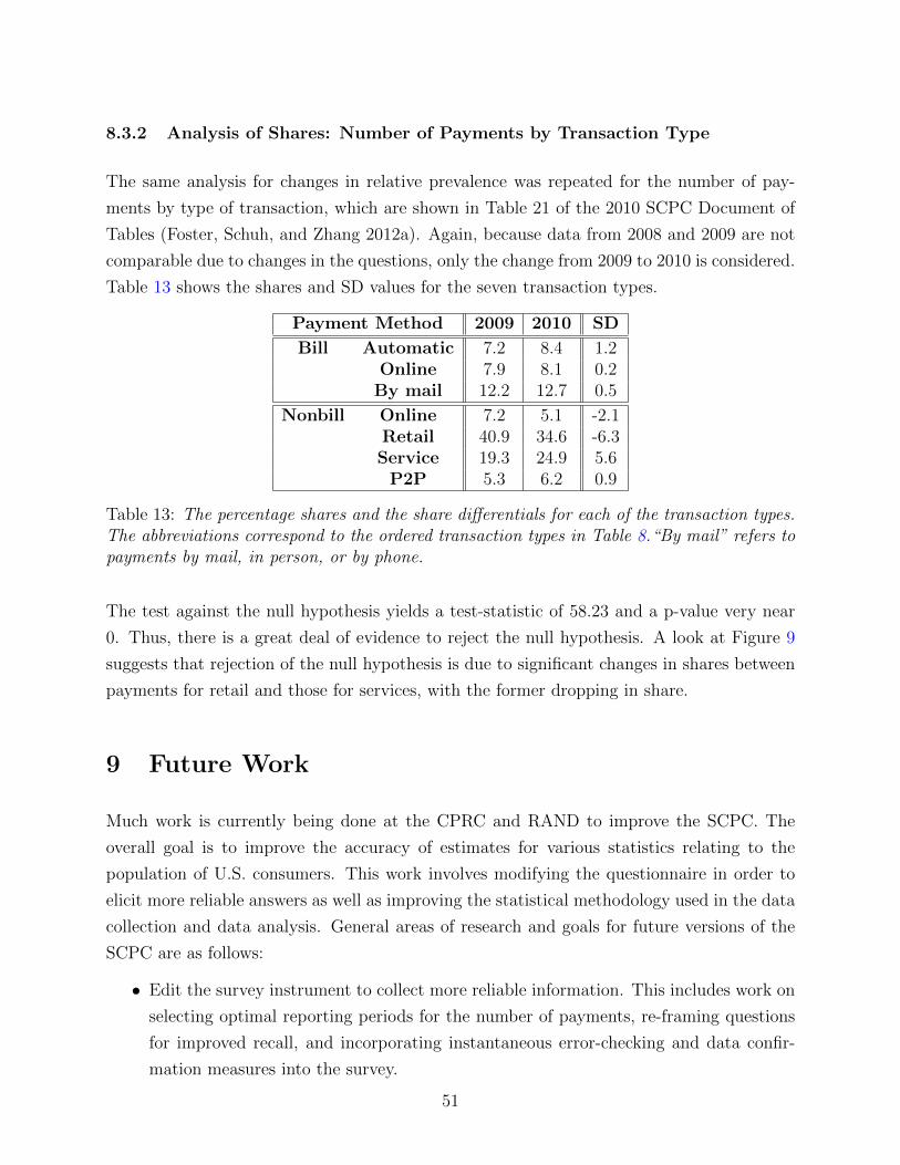
8.3.2 Analysis of Shares: Number of Payments by Transaction Type

The same analysis for changes in relative prevalence was repeated for the number of pay-

ments by type of transaction, which are shown in Table 21 of the 2010 SCPC Document of

Tables (Foster, Schuh, and Zhang 2012a). Again, because data from 2008 and 2009 are not

comparable due to changes in the questions, only the change from 2009 to 2010 is considered.

Table 13 shows the shares and SD values for the seven transaction types.

Payment Method 2009 2010 SD

Bill Automatic 7.2 8.4 1.2Online 7.9 8.1 0.2

By mail 12.2 12.7 0.5

Nonbill Online 7.2 5.1 -2.1Retail 40.9 34.6 -6.3Service 19.3 24.9 5.6

P2P 5.3 6.2 0.9

Table 13: The percentage shares and the share differentials for each of the transaction types.The abbreviations correspond to the ordered transaction types in Table 8.“By mail” refers topayments by mail, in person, or by phone.

The test against the null hypothesis yields a test-statistic of 58.23 and a p-value very near

0. Thus, there is a great deal of evidence to reject the null hypothesis. A look at Figure 9

suggests that rejection of the null hypothesis is due to significant changes in shares between

payments for retail and those for services, with the former dropping in share.

9 Future Work

Much work is currently being done at the CPRC and RAND to improve the SCPC. The

overall goal is to improve the accuracy of estimates for various statistics relating to the

population of U.S. consumers. This work involves modifying the questionnaire in order to

elicit more reliable answers as well as improving the statistical methodology used in the data

collection and data analysis. General areas of research and goals for future versions of the

SCPC are as follows:

• Edit the survey instrument to collect more reliable information. This includes work on

selecting optimal reporting periods for the number of payments, re-framing questions

for improved recall, and incorporating instantaneous error-checking and data confir-

mation measures into the survey.

51

●

●

●

●

●

●

●

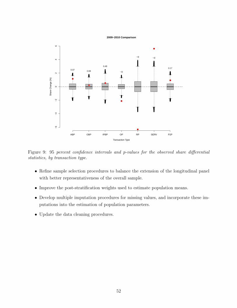
2009−2010 Comparison

Transaction Type

Sha

re C

hang

e (%

)

ABP OBP IPBP OP RP SERV P2P

−6−4

−20

24

6

●

●

●

●

●

●

●

●

●●

●●

●●●●●

●

●

●

●

●

●

●

●

●

●

●

●●

●●●

●●

●●●●

●

●●

●●

●●●●●

●

●

●

●

●

●

●

●●●●●

●●

●●

●

●

●

●

●

●

●●●

●

●

●

●

●●

●

●

●

●

●

●

●

●

●●

●●

●●

●

●

●

●

●

●

●

●

●

●

●●●

●

●

●

●●

●●●

●

●●

●●●●●

●●●●

●

●●●

●●●

●●

●

●

●●●

●

●●●●

●

●

●

●

●

●●●●

●

●

●

●●

●

●●

●

●

●

●

●

●●

●

●

●

●

●

●●●●

●

●

●●

●●

●●

●

●●

●●

●

●

●●●

●

●●

●●●●●●

●●

●

●

●●●

●

●

●●

●

●

●●

●●●●●●

●

●

●

●

●

●

●

●

●●●

●

●

●●

●●

●

●

●●●●

●●

●●

●●

●

●

●●●

●

●

●

●

●

●

●

●●●●●

●

●●

●

●

●●●●

●

●

●

●

●●●

●●●●●

●

●

●●●

●●

●

●●

●●

●

●●●●●●

●●●

●

●●●●●

●●●

●

●

●●

●

●

●

●●

●

●

●

●

●

●●●●●

●●

●

●

●●

●

●●●

●●

●●

●

●

●●●

●

●●●●

●

●

●

●

●

●

●

●●

●

●

●●

●●

●

●

●●●●

●

●●●

●●

●●

●●

●

●

●●

●●

●

●

●●

●

●●●

●

●

●

●

●

●

●

●

●

●

●

●

●●●●

●

●●

●

●●

●

●●●●●

●

●

●●

●

●

●

●

●

●

●●

●

●

●

●●

●●●

●●●●

●

●

●

●

●

●

●●

●●●●●

●

●

●

●

●

●

●

●

●

●

●

●●

●

●●●●

●

●

●

●●

●

●

●

●●●

●●

●●

●

●

●

●

●

●

●

●

●

●

●

●

●

●

●

●

●●

●●●

●

●

●

●

●

●●

●

●

●

●

●●●

●●

●

●

●

●●

●

●

●

●

●

●

●

●

●

●

●

●

●

●●●

●

●

●

●

●

●●●●●

●●

●

●

●

●

●

●

●

●●

●

●

●

●

●

●●

●

●

●

●●

●

●

●

●

●

●

●●

●

●●●●

●

●●

●

●

●

●

●●●●

●●●

●●

●●●

●●

●●●

●

●

●

●

●●●

●●

●

●

●●●●●●

●

●●●

●

●

●

●

●●

●●●

●

●

●●

●

●●

●

●

●●

●●

●

●

●

●

●

●●

●

●

●

●

●●

●●

●●

●

●

●●●

●

●

●

●

●●

●

●●●●

●●●●●●

●

●

●

●

●

●

●●●

●

●

●

●

●●●●

●

●

●

●

●

●●●●

●●

●

●

●

●

●●●●●

●

●●●●

●

●●

●

●

●

●

●

●●●

●

●●

●●●●

●

●

●●

●

●

●

●

●

●

●

●

●

●

●●

●

●

●

●

●●

●●

●

●

●

●

●

●

●

●

●●

●

●

●

●

●

●

●

●

●●

●●

●

●

●

●

●

●

●

●●●

●

●

●

●

●

●

●

●●

●

●

●

●

●●

●

●

●

●●

●

●

●

●

●

●

●

●

●

●

●●

●●

●

●

●

●

●

●

●

●

●

●

●

●

●

●●●

●

●

●

●

●●

●

●

●

●

●

●

●

●

●

●

●

●

●

●

●

●

●

●●

●

●

●

●●

●●

●

●●●

●

●

●

●

●

●

●

●

●

●

●

●

●

●

●

●

●

●●●●

●

●

●

●

●

●●

●●

●

●

●

●

●

●

●

●

●

●

●

●

●

●

●

●

●

●

●●

●●●●

●

●

●

●

●●●●

●

●

●

●

●

●●●

●

●

●

●

●●●

●

●

●●

●●

●●

●

●

●●

●●

●●

●

●

●

●

●

●●

●

●

●

●

●●

●

●

●

●

●

●

●

●●

●

●

●●●

●●

●

●

●●

●

●

●

●

●

●

●

●●

●

●

●

●

●●

●

●

●

●●

●

●

●●

●

●●

●●

●●●●

●

●

●●

●

●

●●●

●

●

●

●●

●

●

●●

●

●●

●●●

●

●

●

●

●●

●

●

●

●●

●

●

●

●●

●

●

●

●

●

●

●

●

●

●

●

●

●

●

●

●

●

●

●

●●

●

●

●

●

●

●

●

●

●

●

●●●

●

●

●

●

●●

●●

●●

●

●

●

●

●●

●

●

●●

●●●

●

●

●

●

●●

●●

●

●

●

●●

●

●●●

●

●

●●●

●

●●●

●

●

●

●●

●

●

●

●

●

●

●●●●

●

●

●

●

●

●●

●●●●

●

●●

●●

●

●

●

●●●

●●

●

●

●●●

●

●

●

●●

●

●●●

●

●

●

●

●

●

●

●

●

●

●

●

●●●●

●

●●

●

●●

●

●

●

●

●

●

●

●●●

●

●●●

●

●

●

●●

●

●

●

●

●

●

●

●●●

●

●

●

●

●

●

●

●●

●

●

●

●●

●

●

●

●

●

●

●

●

●

●

●

●

0.070.69

0.49

~0

~0 ~0

0.17

Figure 9: 95 percent confidence intervals and p-values for the observed share differentialstatistics, by transaction type.

• Refine sample selection procedures to balance the extension of the longitudinal panel

with better representativeness of the overall sample.

• Improve the post-stratification weights used to estimate population means.

• Develop multiple imputation procedures for missing values, and incorporate these im-

putations into the estimation of population parameters.

• Update the data cleaning procedures.

52

References

Angrisani, Marco, Arie Kapteyn, and Scott Schuh. 2013. “Measuring Household Spend-

ing and Payment Habits: The Role of ’Typical’ and ’Specific’ Time Frames in Survey

Questions.” .

Baltagi, Badi H. 2008. Econometric Analysis of Panel Data. Hoboken, New Jersey: John

Wiley and Sons.

Bollen, Kenneth A. and Robert W. Jackman. 1990. “Regression Diagnostics: An Expository

Treatment of Outliers and Influential Cases.” In Modern Methods of Data Analysis, edited

by John Fox and J. Scott Long. Newbury Park, CA: Sage, 257–291.

Bricker, Jesse, Arthur B. Kennickell, Kevin B. Moore, and John Sabelhaus. 2012. “Changes

in U.S. Family Finances from 2007 to 2010: Evidence from the Survey of Consumer

Finances.” Federal Reserve Bulletin 98(2).

Bureau of Labor Statistics. 2013. “Consumer Expenditures and Income.” In BLS Handbook

of Methods. BLS Publishing.

Casella, George and Roger L. Berger. 2002. Statistical Inference. California: Thomson

Learning.

CES. Various Years. “Consumer Expenditure Survey.” http://www.bls.gov/cex/home.

htm.

Chambers, Raymond L. and Ruilin Ren. 2004. “Outlier Robust Imputation of Survey Data.”

The Proceedings of the American Statistical Association .

Cook, R. Dennis. 1977. “Detection of Influential Observations in Linear Regression.” Tech-

nometrics 19(1):15–18.

Cook, R. Dennis and Sanford Weisberg. 1982. Residuals and Influence in Regression. New

York, New York: Chapman and Hall.

CPS. 2010. “Current Population Survey.” http://www.census.gov/cps/.

Daamen, Dancker D. L. and Steven E. de Bie. 1992. “Serial Context Effects in Survey

Interviews.” In Context Effects in Social and Psychological Research, edited by Norbert

Schwarz and Seymour Sudman. Springer-Verlag, 97–113.

DCPC. Various Years. “Diary of Consumper Payment Choices.”

53

De Leeuw, Edith D. 2005. “To Mix or Not to Mix Data Collection Modes in Surveys.”

Journal of Official Statistics 21 (5):233–255.

Deming, W. Edwards and Frederick F. Stephan. 1940. “On a Least Squares Adjustment of a

Sampled Frequency Table When the Expected Marginal Tables are Known.” The Annuals

of Mathematical Statistics 11:427–444.

Duncan, Greg J. and Graham Kalton. 1987. “Issues of Design and Analysis of Surveys Across

Time.” International Statistical Review 55:97–117.

Eicker, F. 1967. “Limit Theorems for Regression with Unequal and Dependent Errors.”

Proceedings of the Fifth Berkeley Symposium on Mathematical Statistics and Probability

:59–82.

Foster, Kevin. 2013. “2010 SCPC Data User’s Guide.” Tech. rep., Consumer Payment

Research Center, Federal Reserve Bank of Boston.

Foster, Kevin, Erik Meijer, Scott Schuh, and Michael A. Zabek. 2011. “The 2009 Survey of

Consumer Payment Choice.” Federal Reserve Public Policy Discussion Papers .

Foster, Kevin, Scott Schuh, and Hanbing Zhang. 2012a. “2010 SCPC Document of Tables.”

http://www.bostonfed.org/economic/cprc/SCPC.

———. 2012b. “The 2010 Survey of Consumer Payment Choice.” Federal Reserve Public

Policy Discussion Papers .

Frees, Edward W. 2004. Longitudinal and Panel Data: Analysis and Applications in the

Social Sciences. Cambridge, UK: Cambridge University Press.

Friedman, Hershey, Paul Herskovitz, and Simcha Pollack. 1994. “Biasing Effects of Scale-

Checking Style in Response to a Likert Scale.” Proceedings of the American Statistical

Association Annual Conference: Survey Research Methods :792–795.

Gelman, Andrew and Hao Lu. 2003. “Sampling Variances for Surveys with Weighting, Post-

stratification, and Raking.” Journal of Official Statistics 19(2):133–151.

Gouskova, Elena, Steven G. Heeringa, Katherine McGonagle, and Robert F. Schoeni. 2008.

“Panel Study of Income Dynamics: Revised Longitudinal Weights 1993-2005.” Tech. rep.,

Survey Research Center, Institute for Social Research, University of Michigan.

Hitczenko, Marcin. 2013a. “Modeling Anchoring Effects in Sequential Likert Scale Ques-

tions.” Tech. rep., Consumer Payment Research Center, Federal Reserve Bank of Boston.

Forthcoming.

54

———. 2013b. “Optimal Recall Period Length in Consumer Payment Surveys.” Tech. rep.,

Consumer Payment Research Center, Federal Reserve Bank of Boston. Forthcoming.

Huber, Peter J. 1967. “The Behavior of Maximum Likelihood Estimates Under Nonstandard

Conditions.” Proceedings of the Fifth Berkeley Symposium on Mathematical Statistics and

Probability :221–233.

Little, Roderick J. A. and Donald B. Rubin. 2002. Statistical Analysis with Missing Data.

New York, New York: Wiley.

Lohr, Sharon L. 1999. Sampling: Design and Analysis. California: Brooks/Cole Publishing.

Lynn, Peter. 2009. Methodology of Longitudinal Surveys. Hoboken, New Jersey: John Wiley

and Sons.

Press, William H., Saul A. Teukolsky, William T. Vetterlin, and Brian P. Flannery. 2007.

Numerical Recipes: The Art of Scientific Computing. New York, New York: Cambridge

Univeristy Press, 3 ed.

SAS Institute Inc. 1999. SAS/STAT User’s Guide, Version 8. SAS Institue Inc., Cary, NC.

SCF. Various Years. “Survey of Consumer Finances.” http://www.federalreserve.gov/

econresdata/scf/scfindex.htm.

White, Halbert. 1980. “A Heteroskedasticity-Consistent Covariance Matrix Estimator and

a Direct Test for Heteroskedasticity.” Econometrica 48(4):817–838.

55