The ArcGIS Coastal Sediment Analyst: A Prototype Decision Support Tool for Regional Sediment Management

John P. Wilson Daniel W. Goldberg Christine S. Lam University of Southern California GIS Research Laboratory Technical Report No. 3 Prepared for: U.S. Army Corps of Engineers

Los Angeles District 915 Wilshire Boulevard Los Angeles, CA 90017

Cover Photo: Carpinteria State Beach, September 2003 (Y. Poon) Preferred Citation: Wilson J. P, Goldberg D. W., and Lam C. S. 2004. The ArcGIS Coastal Sediment Analyst: A Prototype Decision Support Tool for Regional Sediment Management. Los Angeles, Califor-nia: University of Southern California GIS Research Laboratory Technical Report No. 3

Table of Contents Executive Summary......................................................................................................................1

Background....................................................................................................................................3

Study Authority ....................................................................................................................3

Scope and Purpose................................................................................................................3

Study Participation and Coordination...............................................................................4

Model Overview and Data Inputs..............................................................................................4

Model Calculations and User Interface .....................................................................................9

Step 1 – Start CSA Application and Load Geospatial Data ............................................9

Step 2 – Select Harbor and Number of Scenarios...........................................................10

Step 3 – Select Candidate Beaches for Placement of Dredged Sediment....................11

Step 4 – Select Transportation and Disposal Methods ..................................................13

Step 5 – Configure Transportation Options ....................................................................16

Step 6 – Review Transportation Cost Estimates .............................................................23

Step 7 – Select Method Used to Calculate Economic Benefits ......................................24

Step 8 – Review Economic Impact Results ......................................................................27

Steps 9 & 10 – Calculate and Display Final Cost-Benefit Ratios ..................................28

Results, Limitations, and Shortcomings ..................................................................................31

Conclusions..................................................................................................................................37

Literature Cited ...........................................................................................................................39

Appendix A – Coastal and Economic Analyses .....................................................................41

This page left blank intentionally

1

Executive Summary This report describes a prototype GIS-based model that is able to describe the complex, spatially dependent relationships between the cost of sediment transportation and asso-ciated (locally specific) benefits that relocation will generate in a semi-quantitative manner. The development of the Coastal Sediment Analyst prototype required the preparation of a series of custom Visual Basic programs that were integrated with the ArcGISTM geographic information system software (Environmental Research Systems Institute, Inc., Redlands, California) to create an end-user interface that allows users to pick candidate dredge and disposal sites. The user is also able to specify their preferred dredging method, conveyance system, disposal strategy, etc. The tools utilize a series of specially developed response functions by integrating them with the geospatial datasets and user-specific inputs to calculate the costs and benefits of different dredging and disposal options. Ventura Harbor and several nearby beaches in California were used to develop and test this new model. The current version of the Coastal Sediment Analyst (CSA) prototype incorporates a single user interface, an elaborate series of on-line help documents, and various error catching routines. This new tool produced similar results to those reported by Everest International Consultants (EIC) – there were small differences because the new tool cal-culated the transportation distances from the underlying geospatial datasets and these lengths were slightly different than those used by EIC, because of different assumptions that were used to estimate project mobilization/demobilization costs when two or more candidate beach sites were considered, and because different assumptions were used to estimate the recreational benefits of adding additional beach width at Oxnard Shores. There are, however, four sets of limitations and shortcomings with the current proto-type that would need to addressed in order to use this type of tool to analyze conditions at other California harbors and beaches. First, the geospatial datasets describing the harbors, beaches, rail and road network would need to be expanded to cover the entire California coast. Second, some additional data and/or functions describing the histori-cal dredging patterns at other harbors and the sediment budgets at specific beaches would need to be compiled and accessed by the CSA tool. Third, the unit costs for the final two additional dredging and conveyance methods included in the current CSA tool would need to be fleshed out. Fourth, some additional data and/or functions de-scribing the current number of beach visitors and their spending behavior and how these attributes could be expected to change with changes in beach width over time at specific beaches would need to be compiled and accessed by the CSA tool.

The current Coastal Sediment Analyst prototype will be presented to focus workgroups to seek input from local, State, and Federal agencies on the potential uses and ways to improve the model in the immediate future.

2

This page left blank intentionally

3

Background The National Regional Sediment Management (RSM) Program aims to develop meth-odologies and protocols to address and abate site-specific shoreline erosion problems at regional scales. The U.S. Army Corps of Engineers, Los Angeles District is responsible for implementing the California component of the national program. This report pre-sents a study conducted in support of the California component to build a prototype or pilot GIS-based model to perform cost-benefit analysis for different dredging and mate-rial placement options related to maintenance dredging. Study Authority This particular study was conducted in accordance with the National Shoreline Erosion Control Development and Demonstration Program (Section 227) of the Water Resource and Development Act of 1996. Scope and Purpose One of the ultimate goals of the RSM is to develop a GIS-based management support tool for decision makers to evaluate future dredging and disposal options along the California coast. As a first step to achieve this goal, the present study aimed to develop a prototype or pilot GIS model to demonstrate the concept of using GIS as a decision making tool. Through the development of this pilot study, the model architecture, data structures, data requirements, and model interface were specified and tested. This pro-totype model will be presented to focus workgroups to seek input from local, State, and Federal agencies on the potential uses of the model and ways to improve the model. The prototype GIS model presented in this report utilizes the Ventura Harbor dredging and disposal operation along with the placement of beach fill at three beach locations other than McGrath Beach or South Beach (the normal disposal areas) as examples to illustrate the potential strengths and weaknesses of building these types of GIS applica-tions. The following tasks were performed to accomplish the goals of this study:

A series of cost functions for dredge material disposal was created. The benefits associated with placing the dredged material from Ventura Harbor

on three alternative beach fill sites were calculated. The differential costs versus regional benefits for the three selected beach fill sites

were estimated.

4

The results of the differential cost-benefit analysis were incorporated into a proto-type GIS-based model that can be used to perform this same type of analysis.

It has to be noted that the placement scenarios presented in the report were for illustra-tion only, and are not intended to be "real-world" projects that could implemented as specified in this report. In addition, the cost functions and benefit analyses were done at a crude level with broad assumptions to cover a wide range of possible transportation and disposal scenarios to test the prototype GIS-based model; hence, the examples in-corporated in this report should not be viewed as sufficient analyses for the specifica-tion of one or more "real-world" site-specific scenarios. Study Participation and Coordination This study is part of the California Coastal Sediment Management Master Plan, which is a collaborative effort between federal, state, local agencies and non-governmental or-ganizations. Everest International Consultants Inc., (EIC) based in Long Beach, Califor-nia, supported the work performed by the University of Southern California (USC) GIS Research Laboratory. Dr. Philip King, Department of Economics, San Francisco State University, also participated in this project. EIC performed coastal engineering evaluation for the three beach sites and prepared the cost functions from published literature and interviews. Dr. King provided the analysis of the recreational benefits associated with placing sediment at the proposed sites. His analysis relied on numerous visits to the three sites as well as the results of several visi-tor surveys that were conducted specifically for this project. Dr. King also incorporated results from other studies of California beaches and applied the U.S. Army Corps of Engineers methodology for estimating recreational value. The three authors of this report then used the results laid out in Appendix A – Coastal and Economic Analyses prepared by EIC to develop the prototype or pilot GIS-based model that could, with some additional modifications, be used to evaluate future dredging and disposal options along the California Coast.

5

Model Overview and Data Inputs The USC GIS Research Laboratory was contracted to build a prototype ArcGIS model (referred to hereafter as the "CSA" or "Coastal Sediment Analyst") that is able to de-scribe the complex, spatially dependent relationships between the cost of sediment transportation and the associated (locally specific) benefits that relocation will generate in a qualitative or semi-quantitative manner. These capabilities meant, in turn, that at least two environments were to be characterized in the GIS – one for the nearshore envi-ronment and the second for the local beaches with attributes to support the response functions described below. Ventura Harbor and several nearby beaches in California were used to develop and test this new model, which was expected to take local littoral processes, beach conditions specific to Ventura Harbor in relation to dredged sediment volume, dredge equipment and current operation costs into account, and to be able to automatically update the calculated benefit values in a near real time manner. Various model constraints posed by significant physical, economic, geomorphic, and spatio-temporal variables considered relevant for the methodology developed were to be iden-tified and specified in this final report. The completion of this prototype required the preparation of a series of custom Visual Basic programs (called scripts) that can be integrated with ArcGISTM (Environmental Research Systems Institute, Inc., Redlands, California) to create an end-user interface that allow users to pick candidate dredge and disposal sites. The user interface was de-signed in such a way that the user is able to specify their preferred dredging method, conveyance system, disposal strategy, etc. The tools utilize the response functions by integrating them with the geospatial datasets and user-specific inputs to calculate the costs and benefits of different dredging and disposal options. Two sets of response functions were extracted from Appendix A and used to construct the prototype tools described in this report as follows:

A series of response functions that described the costs of different dredging and disposal operations at Ventura Harbor. These response functions were to be specified in such a way that they could compute the differential cost of transport-ing and disposing of Ventura Harbor dredge material from the traditional dis-posal sites used by the Engineers Operations and Maintenance Division of the Los Angeles District Army Corps versus the cost of disposing of these materials at three alternative sites identified as erosional hot spots by the Los Angeles Dis-trict Corps of Engineers in conjunction with the State of California Department of Boating and Waterways for this pilot project.

A series of response functions that described the site-specific and regional bene-fits of several different sediment deposition strategies. These response functions were to be specified in such a way that they reflect site-specific benefits due to conditions such as beach width and rate of beach accretion-regression. This new benefit curve function was to consider the benefits derived from recreation,

6

storm damage reduction, protection of public facilities and infrastructure, tax revenue, creation of jobs, environmental enhancement, and other factors that were found to be relevant during the literature review and/or development of the methodology itself.

The various forms incorporated in the user interface are user friendly and capable of providing non-GIS users with clearly defined data entry options, analysis tools, and relevant reference information (i.e. an online Help system). The analysis tools facilitate the comparison of the various dredging and conveyance options for Ventura Harbor in a systematic and reproducible manner, incorporating near real-time sediment data. The ultimate goal is to develop a suite of tools that are applicable to other localities with similar environmental characteristics. Thus, when completed, the final system should be able to be used in similar locations in coastal California under the jurisdiction of the Los Angeles District of the U.S. Army Corps of Engineers and places further afar. This final report gives some indication as to the further GIS work and/or data required to support the application of this prototype model in these other locations. The following scenarios and inputs were used for the initial development of the tools and beta demonstration provided for Los Angeles District Corps of Engineers staff at the USC GIS Research Laboratory on 7 April 2004. The names listed below in square brackets correspond to the tabs used for the Coastal Sediment Analyst user interface (see Figures 1 through 17 for actual examples): [Harbor] User is required to specify following inputs:

Name of harbor – Ventura

Number of scenarios – 4

[Beaches] User is required to specify following inputs:

Scenarios – #1 – 450,000 cubic yards of sediment to Carpinteria #2 – 275,000 cubic yards of sediment to Oil Piers – 175,000 cubic yards of sediment to Carpinteria #3 – 450,000 cubic yards of sediment to Oxnard Shores #4 – 150,000 cubic yards of sediment to Carpinteria, Oil Piers, and Oxnard Shores

Current beach width – 150 feet (Carpinteria) 50 feet (Oil Piers)

7

250 feet (Oxnard Shores)

Increase in beach width (one year from date when new beach fill is first applied) – 119 feet (Carpinteria; 450,000 cubic yards of sediment added) 46 feet (Carpinteria; 175,000 cubic yards of sediment added) 40 feet (Carpinteria; 150,000 cubic yards of sediment added) 65 feet (Oil Piers; 275,000 cubic yards of sediment added) 35 feet (Oil Piers; 150,000 cubic yards of sediment added) 80 feet (Oxnard Shores; 450,000 cubic yards of sediment added) 27 feet (Oxnard Shores; 150,000 cubic yards of sediment added) [Trans Opts] User is required to specify following inputs:

Transportation and disposal methods – Railroad Scow and tow Truck [Trans Config] Defaults provided with Coastal Sediment Analyst used for railroad option.

User is required to specify number and types (sizes) of scow and tow units that will be used when this option is chosen – we specified 2 large scow units and 1 large and 2 small tow units (to match the scenarios used by EIC in Appendix A).

Defaults provided with Coastal Sediment Analyst used for truck option. [Trans Cost] No user-specified inputs required. [Econ Config] User is required to specify following inputs:

No. of visitors – 1,900,000 (Carpinteria)

23,100 (Oil Piers) 80,850 (Oxnard Shores)

Total recreation value – $26,572,000 (Carpinteria) $ 184,400 (Oil Piers) $ 727,650 (Oxnard Shores)

Percent Day trippers – 34% (Carpinteria)

100% (Oil Piers) 80% (Oxnard Shores)

8

Overnight visitor spending – $43.54 (all beaches)

Day tripper spending – $13.73 (all beaches)

[Econ Results] [Final Results] [Scenario Comparison]

No user-specified inputs required

9

Model Calculations and User Interface The user starts the program by opening ArcMap and clicking on the Coastal Sediment Analyst (CSA) button on the top row of buttons in ArcMap (Figure 1). From there, the user must complete a series of tasks in a specific sequence (or series of steps) to calculate the benefits and costs associated with various user-specified dredging and material placement options. Step 1 – Start CSA Application and Load Geospatial Data The user clicks on the CSA tool and loads several specially prepared sample data files by clicking on the item with this name in the dropdown list provided with the CSA tool. The completion of this task should result in the display of a map of Southern California with harbors indicated by name (Figure 1).

Figure 1: Geospatial data layers loaded when Coastal Sediment Analyst tool is invoked.

Once these data are loaded, the user can click on Begin Demo in the CSA dropdown list to start the application that ultimately calculates the benefits and costs associated with two or more user-specified dredging and material placement options.

10

Step 2 – Select Harbor and Number of Scenarios The user now chooses a harbor for dredging by clicking on the appropriate harbor name on the map or by clicking on this name in a dropdown list of candidate harbor names in a popup window (Figure 2). Note that the design is such that the user can only select a single harbor at this step. The user must specify the number of scenarios that they wish to evaluate at this step as well. Alternatively, the user can open an existing model by clicking on File>Open Model from this tab. These models specify one or more existing (i.e. preset) scenarios. The choice of candidate beaches and transportation methods should not be modified if the user chooses this option. However, the user can select one or more methods to calculate the economic benefits and modify the beach input data (Step #6 below) when they choose this option. The user can save a model at any time by clicking on File>Save Model to File. This op-tion can be invoked to distribute the various work tasks described below over multiple sessions and/or to review past work.

Figure 2: Map display and popup window used to select harbor for dredging.

11

The completion of these tasks will produce a new map centered on the selected harbor with a new annotation layer indicating the names and approximate locations of candi-date beaches displayed. The beach names in this new map are distinguished from the harbor names using a different font size and color (see Figure 3 for details). Step 3 – Select Candidate Beaches for Placement of Dredged Sediment The user next chooses one or more candidate beaches for the placement of the dredged sediment by clicking on the appropriate beach names on the map or by clicking on these names in a dropdown list of candidate beach names (Figure 3). The user must also specify the annual volume of sediment to be dredged in cubic yards for the previously selected harbor and numerous details about each of the candidate beaches at this step. The Help tool provided at the bottom right of this popup window (see Figure 4 for details) can be used to review information on historical maintenance dredging and costs for the selected harbor (i.e. Ventura Harbor in this example) if this information is available.

Figure 3: Map display and popup window used to select candidate beaches.

12

Figure 4: Popup window used to specify sediment volumes and beach widths.

The user next chooses the volumes of sediment to be placed at each of the candidate beaches under each scenario (Figure 4). The volumes entered at this step are checked by the program for logical consistency at two levels. The first level is focused on individual beaches since there is an upper limit as to the volume of sediment that can be placed at some sites. Two of the beaches (Carpinteria and Oxnard Shores) had no upper limit, but the third (Oil Piers) could only handle volumes of ≤ 275,000 cubic yards in the applica-tion used to build and test the Coastal Sediment Analyst tool for example. The second level focused on the total volume of sediment allocated to the candidate beaches under each scenario since these totals cannot exceed the total volume to be dredged at the se-lected harbor. The user must also specify or estimate the current beach width and (possibly) the change in beach width anticipated for different volumes of beach fill at this step. The change in beach width will be calculated for them if the appropriate information is stored in a file – otherwise a warning is issued and the user is expected to specify an appropriate value in this box as well. The Help tool provided at the top right of this popup window (see Figure 4 for details) can be used to review beach information (if available). The file that is chosen and opened here will match the beach highlighted in the dropdown list of beach names on the left side of this popup window. The user has to hit Store Values for each of the beaches or the values will not be stored and used at subsequent steps. The beach widths are important and will be used later along with the current recreational value of beaches, discount rate, and information on beach width losses due to erosion to calculate the additional beach widths present at specified inter-vals over a 20-year period.

13

The completion of the tasks for step #3 will take more time than most steps because unique values will often need to be specified by the user for both the volume of sedi-ment and increase in beach width for each of the beaches in each of the scenarios to be evaluated with the CSA tool. Step 4 – Select Transportation and Disposal Methods The user must complete two sets of tasks at this step. The first is to select one or more transportation and disposal methods from the drop-down list (Figure 5). The Help button in this popup window provides additional infor-mation about the five transport and disposal methods in the dropdown list (i.e. hopper dredge and pump out, hydraulic pipeline, railroad, scow and tow, and truck) although the current version of the CSA tool can only calculate the costs of using the final three methods in this list.

Figure 5: Popup window used to select transport and disposal methods.

The second task will depend on the currently selected transport and disposal method since this will determine what the user must do next to identify the transportation routes that will be used in all subsequent calculations.

14

For the railroad option, the user is prompted to select the origin (near Ventura Harbor) for the transport of the sediment on the existing railroad network and one of the candi-date beach fill destinations (Figure 6). This task must be repeated for each of the origin-destination pairs. The CSA tool will then calculate the distances of the shortest paths along the network for each unique origin-destination pair and store this result in a table because these distances will be utilized later to calculate the cost of using trains to transport and dispose of the dredged sediment at each of the candidate beaches.

Figure 6: Railway network used to specify harbor (i.e. origin) and beach fill destinations.

For the scow and tow option, the user is prompted to select an origin (some location inside the harbor selected earlier) and then draw routes across the ocean from this ori-gin to each of the previously specified destinations (i.e. the midpoints of the candidate beaches selected earlier). The CSA tool then displays these lines on the map (Figure 7), calculates the length of each of these paths, and stores the results in a table since these distances will be used later to calculate the cost of using the scow and tow option to transport and dispose of the sediment at each of the candidate beaches. For the truck option, the user is prompted to select an origin (near Ventura Harbor) and one of the beach fill destinations for the transport and disposal of this sediment using the road network (Figure 8). This task must be repeated for each of the origin-destination pairs. The CSA tool will then calculate the shortest paths along the network for each unique origin-destination pair and store this result in a table because these dis-tances will be used later to calculate the cost of using trucks to transport and dispose of dredged sediment at each of the candidate beaches.

15

Figure 7: Scow and tow route drawn between harbor to be dredged and candidate beach.

Figure 8: Road network used to specify harbor (i.e. origin) and beach fill destinations.

16

Step 5 – Configure Transportation Options The user must specify certain costs at this step for the CSA tool to calculate the trans-port and disposal costs that would be incurred under each of the scenarios specified earlier. The default values shown in Figures 9, 10 and 11 were compiled from the results summarized in Appendix A. The user can review some additional information on the available options in a separate popup window by clicking on the Help button in Figures 9, 10 and/or 11 as well. Separate solutions are required for each transport and disposal option investigated and the text that follows summarizes the various input data needed for each of the three transport and disposal options incorporated in the current CSA tool. The values entered for each transport and disposal option are global – which means they apply to all of the beaches that utilize a particular transport and disposal method in a particular scenario. For the railroad option, the basic approach involves separating fixed and variable costs, calculating each component separately, and then summing these components for each destination in each of the scenarios. Sample assumptions and calculations are shown in italics and square brackets at the end of each task below to help illustrate the calcula-tions that are performed.

Determine cost of mobilization and demobilization (for transport and disposal only) per cubic yard of sediment to be placed at one or more destinations (i.e. beach fill sites). The user is given the option of specifying the project mobiliza-tion and demobilization costs, although $100,000 per dredging project is speci-fied as the default (Figure 9). This cost is allocated to multiple destinations on a proportional basis for those scenarios that anticipate transport and disposal of dredged sediment at two or more destinations.

[Assume cost of $100K per project and that there is 150,000 cubic yards of sediment to place at two or more candidate beaches – mobilization and demobilization cost is $0.67 per cubic yard]

Determine volume of sediment that can be moved in a single day. The user is given the option of specifying the size of the train to be used, although trains with 40 cars, 4 containers per car, and 20 ton containers are specified as the de-fault (Figure 9). Three trains are needed to implement this option – one train is loaded at the origin (i.e. dredge site) each day, the second train is in motion moving the dredged sediment from the origin to the destination, and the third train is being unloaded at the destination (i.e. beach fill site).

[Assume a train with 40 cars, 4 containers per car, 20 ton loads per container, and that 1 cubic yard of sediment weighs 1.4 tons – volume of sediment that can be moved in a single day is 2,286 cubic yards]

17

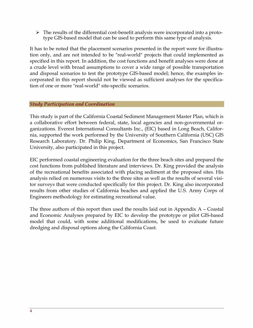
Figure 9: Popup windows used to specify railroad cost information.

Determine loader and dozer costs per cubic yard of sediment to be placed at one or more candidate beach fill sites. The user is given the option of specifying these costs, although loader and dozer costs of $1,400 per unit per day are speci-fied as default values (Figure 9). The user must hit Store for each of the trans-port methods at this moment or the values that they just entered will be not be stored for later use.

[Assume loader costs of $1,400 per day and dozer costs of $1,400 per day – loader/dozer cost is $1.22 per cubic yard]

Determine number of days required to move total volume of sediment from the origin (i.e. harbor to be dredged) to each of the destinations (i.e. candidate beach fill sites) envisaged in each of the scenarios. Add one to this answer and then truncate it (this is same as taking original estimate and rounding it up to next highest integer).

[Assume that 150,000 cubic yards of sediment is to be moved – 150,000 / 2,286 = 65.62 so answer here is 66 days]

Sum the fixed costs calculated for this option.

[The fixed costs are $0.67 + $1.22 = $1.89 per cubic yard of sediment moved given the assumptions used in this example]

18

Determine variable costs of transporting sediment for this option. This calcula-

tion could have been accomplished in a variety of ways – the method outlined below relies on a series of IF THEN statements that are used with the distance the sediment needs to be moved (these distances were determined in the previ-ous step and the statements below rely on variables labeled DST and VCT to represent the distance sediment must be transported and the variable costs, re-spectively).

IF (DST ≤ 50) THEN VCT = 36.00 IF (DST > 50 AND DST ≤ 100) THEN VCT = 36.00 + 0.04 * (DST – 50) IF (DST > 100 AND DST ≤ 150) THEN VCT = 36.00 + 0.02 * (DST – 50) IF (DST > 150) THEN VCT = 36.00 + 0.0133 * (DST – 50)

[Assume 75 mile trip – the CSA tool will use the second of the aforementioned IF THEN statements and estimate variable costs of $37.00 per cubic yard in this example]

Determine total cost of using this option by summing the fixed and variable costs calculated in the two previous steps.

[Total cost of transporting and disposing of 150,000 cubic yards of sediment at a beach 75 miles from the dredge site is $1.89 + $37.00 = $38.89 per cubic yard]

For the scow and tow option, the basic approach once again involves separating fixed and variable costs, calculating each component separately, and then summing these components for each destination in each of the scenarios. Sample assumptions and calculations are shown in italics and square brackets at the end of each task be-low to help illustrate the calculations that are performed.

Determine cost of mobilization and demobilization (for transport and disposal only) per cubic yard of sediment to be placed at one or more candidate beach fill sites and add onshore handling fees. The user is given the option of specifying their own estimates for the project specific mobilization/demobilization and on-shore handling costs, although $300,000 per dredging project and $0.15 per cubic yard are specified as the mobilization/ demobilization and onshore handling default costs, respectively (see Figure 10 for details). The first component of these costs is allocated to multiple destinations on a proportional basis for those scenarios that anticipate transport and disposal of dredged sediment at two or more destinations.

[Assume mobilization/demobilization costs of $300K per project and that there is 150,000 cubic yards of sediment to place at beach fill sites – answer here is $2.00 + $0.15 = $2.15 per cubic yard]

19

Figure 10: Popup windows used to specify scow and tow cost information.

Specify number of hours equipment is used each day and determine volume of sediment that can be moved in a single day. The user is given the option of specifying the number and size of the scows to be used under this option. How-ever, 2 large scows capable of carrying 3.5 tons (2,500 cubic yards) per trip at an average speed of 6 knots (approximately 7 mph; 1 knot = 1.15 mph) and 2 small scows capable of carrying 2,100 tons (1,500 cubic yards) per trip at an average speed of 6 knots (7 mph) are recommended for most California applications.

[Example 1: Assume 2 large scows, 8.5 hours of operation per day, a 3.5 ton load per trip, 1.0 hour to load and 0.5 hour to unload per trip, travel between the origin and des-tination at an average speed of 7 mph and a trip length of 2 miles – volume is 20,530 cu-bic yards per day]

[Example 2: Assume 2 large scows, 8.5 hours of operation per day, a 3.5 ton load per trip, 1.0 hour to load and 0.5 hour to unload per trip, travel between the origin and des-tination at an average speed of 7mph and a trip length of 75 miles – volume is 1,983 cu-bic yards per day. This example is used for the remainder of the calculations for this op-tion below]

Determine variable scow and tow equipment costs per cubic yard of sediment to be placed at one or more candidate beach fill sites – this is a function of the

20

number of days the equipment is required (determined at previous step) and the cost assumptions that are used. The scow and tow costs listed below were speci-fied as defaults for the large scow and large tow defaults and costs of $800 and $3,000 per day were specified as the defaults for the small scow and tow units, respectively (Figure 10). The user will need to hit the Set buttons in Figure 10 when they modify the default values that are displayed with each scow and tow option.

[Assume large scow costs of $2,000 per scow per day and large tow costs of $6,000 per tow per day – answer here is $8.10 per cubic yard for trips of 75 miles; the equivalent cost for trips of 2 miles by way of comparison is only $0.78 per cubic yard]

Determine number of days required to move total volume of sediment from the harbor to be dredged to each of the candidate beach fill sites envisaged in each of the scenarios. Add one to this answer and then truncate it (this is same as tak-ing original estimate and rounding it up to next highest integer).

[Assume that 150,000 cubic yards of sediment is to be moved – 150,000 / 1,983 = 75.64 so answer here is 76 days]

Determine the total cost of using this option. This is simply the sum of the fixed and variable costs calculated in prior steps.

[Total cost of transporting and disposing of 150,000 cubic yards of sediment at a beach 75 miles from the dredge site is $2.15 + $8.10 = $10.25 per cubic yard]

For the truck option, the basic approach is similar to the railroad option and in-volves separating fixed and variable costs, calculating each component separately, and then summing these components for each destination in each of the scenarios. Sample assumptions and calculations are shown in italics and square brackets at the end of each task below to help illustrate the calculations that are performed.

Determine cost of mobilization and demobilization for transport and disposal only per cubic yard of sediment to be placed at one or more candidate beach fill sites. The user is given the option of specifying their own project mobilization and demobilization cost estimates, although $100,000 per dredging project is specified as the default (see Figure 11 for details). This cost is allocated to multi-ple destinations on a proportional basis for those scenarios that anticipate trans-port and disposal of dredge sediment at two or more destinations.

[Assume cost of $100K per project and that there is 150,000 cubic yards of sediment to place at beaches – answer here is $0.67 per cubic yard]

21

Figure 11: Popup windows used to specify truck cost information.

Specify volume of sediment that can be moved in a single day and determine number of trucks that will be needed to move this volume of sediment. This ap-proach assumes that the designated number of trucks is available to move the sediment – for example, 11 trucks capable of carrying 20 tons will be required to move 2,143 cubic yards of sediment for trips of 2 miles or less; 14 trucks will be required for trips of 2-5 miles, 18 trucks will be required for trips of 5-10 miles, 22 trucks will be required for trips of 10-15 miles; 26 trucks will be required for trips of 15-20 miles; 30 trucks will be required for trips of 20-25 miles; 34 trucks will be required for trips of 25-30 miles; 38 trucks will be required for trips of 30-35 miles; and ≥ 54 trucks will be required for trips exceeding 35 miles in length.

[Assume 2,143 cubic yards are moved each day, 8 hours of operation per day, a 20 ton load per trip, 0.5 hour to load and unload per trip, a trip length of 2 miles, and travel be-tween the origin and destination at an average speed of 48 mph – this will require 11 trucks to move this volume of material from the harbor to the beach fill site each day]

Determine loader and dozer costs per cubic yard of sediment. The calculations below assume that 0.25 hour is needed to load and spread each truckload of sediment – hence each loader and dozer can handle 32 trucks per 8 hour day and the CSA tool needs information about the number of trucks to be deployed

22

and average length of each trip to calculate the loader and dozer costs per cubic yard of sediment.

[Example 1: Assume 11 trucks (as above) each making 13.7 trips per day, loader costs of $1,400 per day, dozer costs of $1,400 per day, and a trip length of 2 miles – daily loader and dozer costs are 4.70 x $2,800 = $13,160 giving loader /dozer costs of $6.05 per cubic yard of sediment]

[Example 2: Assume 15 trucks each making 2.2 trips per day, loader costs of $1,400 per day, dozer costs of $1,400 per day, and a trip length of 75 miles – daily loader and dozer costs are 1.03 x $2,800 = $2,890 giving loader /dozer costs of $6.13 per cubic yard of sediment]

Determine truck costs per cubic yard of sediment. The calculations below as-sume that trucks cost $600 per day.

[Example 1: Assume 11 trucks (as above) and that each truck costs $600 per day – daily truck costs are 11 x $600 = $6,600 giving truck costs of $3.08 per cubic yard of sedi-ment]

[Example 2: Assume 15 trucks (as above) and that each truck costs $600 per day – daily truck costs are 15 x $600 = $9,000 giving truck costs of $19.07 per cubic yard of sedi-ment]

Determine number of days required to move total volume of sediment from the harbor to be dredged to each of the candidate beach fill sites envisaged under each of the scenarios. Add one to this answer and then truncate it (this is same as taking original estimate and rounding it up to next highest integer).

[Assume that 150,000 cubic yards of sediment is to be moved and that 2,143 cubic yards is moved each day – 150,000 / 2,143 = 70.00 so answer here is 70 days]

Sum the fixed costs calculated for this option.

[The fixed costs are $0.67 + $6.13 + $19.07 = $25.87 per cubic yard of sediment moved given the assumptions used in example #2]

Determine variable costs of transporting sediment under this option. This calcu-lation could have been accomplished in a variety of ways – the method outlined below relies on two IF THEN statements that are used with the distance the sediment needs to be moved (these distances were determined in the previous step and the statements below rely on variables labeled DST and VCT to repre-sent the distance sediment has to be transported and the variable costs, respec-tively).

IF (DST ≤ 2) THEN VCT = 4.37 IF (DST > 2) THEN VCT = 4.37 + 0.22 * (DST – 2)

23

[Assume 75 mile trip – the CSA tool will use the second of the abovementioned IF THEN statements and estimate variable costs of $20.43 per cubic yard]

Determine total cost of using this option. This is simply the sum of the fixed and variable costs calculated in the two previous steps.

[Total cost of transporting and disposing of 150,000 cubic yards of sediment at a beach 75 miles from the dredge site is $25.87 + $20.43 = $46.30 per cubic yard]

Step 6 – Review Transportation Cost Estimates The costs estimated for the transport and placement of sediment at each of the candi-date beach fill sites (as shown in Figure 12) can be reviewed by the user at this step. The user can review the calculations used to determine the transportation costs by clicking on the appropriate cell in the table displayed in this popup window (Figure 12). The user can also recalculate these costs by modifying the assumptions and/or repeating some or all of the calculations performed at the previous step.

Figure 12: Popup window used to display transportation costs calculated for different candidate

beach fill sites under each scenario.

24

Step 7 – Select Method Used to Calculate Economic Benefits The Coastal Sediment Analyst tool will calculate the benefits that can be attributed to additional beach fill for each of the beaches included in each of the scenarios once the user selects one or both of the methods provided for calculating these benefits and they specify the necessary beach input data at this step. The user starts by selecting one or both of the available methods for calculating the eco-nomic benefits of additional beach fill from the dropdown list at the bottom left corner of the appropriate popup window (see Figure 13 for details). The user can view some background information on the two methods provided for calculating the economic benefits of additional beach fill in a separate popup window by clicking on the Help button located to the right of this dropdown list. In addition, the user is afforded the option of specifying the discount rate that will be used to calculate the economic benefits of additional beach width at this step (Figure 13), although 6% is specified as the default and is recommended for most applications. The user is also shown lists of beaches under each of the scenarios designated earlier (i.e. step #3) and asked to specify the annual number of beach visitors (day-trippers and overnight visitors combined), current recreational value of each beach, percentage of total visits by day-trippers, overnight spending per visitor, and the total spent by day-trippers at this step (see Figure 13 for details). This information can be extracted from the beach descriptions (if available) that can be accessed by clicking on the Help button on the top right-hand side of this popup window (Figure 13). The Coastal Sediment Analyst tool will then calculate the total spending associated with each beach when the user clicks on the Calculate button in the bottom right-hand corner of this same win-dow (Figure 13). The user has to click on Store Values for each of the beaches or the values will not be saved when they finish these tasks. The CSA tool calculates the economic benefits over a 20 year period for each of the sce-narios at the conclusion of this step (see Figure 14 for sample display). The outputs dis-played and calculations that are performed depend on the methods that are chosen for a particular model run. We can assume (for the purposes of this report) that both meth-ods were chosen, and some additional information about the calculations performed by the CSA tool using each of these methods is provided below.

25

Figure 13: Popup window used to select method chosen for calculating economic benefits

and to specify beach use characteristics.

Figure 14: Popup window used to display economic benefits of different dredging and beach

fill placement options with both travel cost and tax impact methods.

26

For the travel cost method, the CSA tool takes the initial increase in beach width for a prescribed volume of beach fill that was provided by the user at an earlier step (#3) to-gether with the beach width retention data saved as a part of the tool to calculate the additional beach width that survives after 1 year, 2 years, 3 years, etc. The percentages listed in the third column of the table (Figure 14) are simply the width from column 2 divided by the initial beach width (i.e. before the beach fill was added) that was speci-fied by the user in step #3. This variable is labeled PC below and is used along with the number of visitors (VISIT) and the recreational value of the specified beach (RVAL) (both of these variables are calculated at this step) to estimate the gain in recreational value (GRV) for each time increment as follows:

NV = PC * (0.2 * VISIT) * ((RVAL/VISIT) + (PC * 0.18 * RVAL/VISIT)) (1)

NS = PC * VISIT * RVAL/VISIT * 0.18 (2)

GRV = NV + NS (3)

The two components shown in the aforementioned equations represent the gain in rec-reational value associated with increased numbers of visitors (NV) and increased spending per visitor per day (NS). The result generated with Equation (3) is displayed in column 4 in the table reproduced in the popup window shown in Figure 14. The pre-sent-day values in the fifth column of this table were then calculated using the user-specified discount rate (RATE) and number of years elapsed (YRS) with the estimated recreational gains (column #4) and the following equation:

PV = GRV / (1 + (RATE / 100))YRS (4)

For the tax impact method, the values in the first three columns of the table in the popup window reproduced in Figure 14 are used along with the number of visitors and total spending to estimate the increase in total spending over the next 20 years. The number of visitors was specified in the current popup window (see Figure 13 for de-tails) and the total spending was calculated from the estimated spending per day-trip visitor, estimated overnight spending per visitor, and percentage of total visits by day-trippers at each beach by the CSA tool. The Coastal Sediment Analyst tool calculates the anticipated increase in total spending (INCR) displayed in column #6 of the aforemen-tioned table in Figure 14 as follows:

INCR = O.2 * WIDTH * SPEND (5)

where WIDTH is the increase in beach width expressed as a percentage of the initial beach width (i.e. before the beach fill was added) and SPEND is the total recreational spending calculated with the CSA tool in the popup window reproduced in Figure 13. This approach provides the user with the best estimates of the increase in total spending anticipated in year 1, year 2, year 3, etc. (see Figure 14 for details). The present value of this increase in total spending (PVINCR) is then calculated using the user-specified dis-

27

count rate (RATE) and number of years elapsed (YRS) and estimated increase in total spending (column #6) as follows:

PVINCR = INCR / (1 + (RATE / 100))YRS (6)

The values in the eighth and final column of the table reproduced in Figure 14 showing the present value of the state tax impact of the additional beach fill are calculated as-suming a state sales tax of 8%. Step 8 – Review Economic Impact Results The benefits estimated for each of the candidate beach fill sites with the travel cost and/or tax impact methods (as shown in Figure 14) can be reviewed by the user at this step. The user can review the calculations used to determine these impacts by clicking on the appropriate cell in the table displayed in this popup window (Figure 14). The user can also recalculate these benefits by modifying the assumptions and/or repeating some or all of the calculations performed at the previous step. The user can also export the results displayed with the [Econ Results], [Final Results], and [Scenario Comparison] tabs to ExcelTM (Microsoft, Seattle, Washington) to facilitate further analysis and/or display. Clicking on this option will cause an error if Excel is open and you try to save the CSA results. The user must choose an Excel file that is not already open and in use to successfully complete this particular task. Steps 9 & 10 – Calculate and Display Final Cost-Benefit Ratios for Each Scenario The Coastal Sediment Analyst tool produces one summary table for each scenario (step 9; see Figure 15 for details) and one table combining all of the scenarios that were con-sidered in the preceding analysis (step 10; see Figure 16 for details). The final layout of these tables and additional work required to produce each of these tables is described below. The first row in the first table lists the beach fill sites included in each scenario. The sec-ond row lists the least cost for transporting and disposing of the designated volume of dredged sediment at each of these beach fill sites. The third row reports the present value of the additional recreational benefits calculated with the travel cost method (step #7) summed over 20 years (this approach means that the estimated value for year 0 was not used for the cost-benefit calculations). The ratio of recreational benefits and costs is then calculated and written in the fourth row in each of these tables. Ratios > 1 indicate situations where the benefits exceed the costs. Ratios < 1 indicate situations where the

28

costs of transporting and placing sediments at these beach fill sites exceeds the benefits calculated with the travel cost method.

The fifth row in both tables reports the present value of the increase in total spending calculated with the tax impact method (step #7) summed over 20 years (so that the es-timated value for year 0 was not used for these cost-benefit calculations as noted ear-lier). The ratio of increased spending and cost is then calculated and written in the sixth row of both tables. These values will probably exceed 1 for every beach fill option con-sidered because they measure the ratio of increased spending attributed to wider beaches and the cost of transporting and placing sediment at each of the candidate beach fill sites. The seventh row in both tables reports the present value of the increase in state tax revenues calculated with the tax impact method (step #7) summed over 20 years (so that the estimated value for year 0 was not used for these cost-benefit calculations ei-ther). The ratio of increased state tax revenues and cost is then calculated and written in the eighth and final row of this pair of tables. Ratios > 1 indicate situations where the increase in state tax revenues exceeds the costs. Ratios < 1 indicate situations where the costs of transporting and placing sediments at these beach fill sites exceeds the increase in state tax revenues calculated with the travel cost method. The final table in the popup window reproduced in Figure 16 shows the same informa-tion summed by scenario. The two rows that show the recreational benefit/cost and state tax revenue increase/cost ratios (rows #4 and #8, respectively) will attract the most attention and can be used to compare the financial consequences of the different scenarios specified by the user when they first invoked the Coastal Sediment Analyst tool.

29

Figure 15: Popup window showing various cost-benefit ratios for different beach fill options.

Figure 16: Popup window showing various cost-benefit ratios for different scenarios.

30

This page intentionally left blank

31

Results, Limitations, and Shortcomings Tables 1 through 4 show the various benefits and costs generated with the new Coastal Sediment Analyst tool and the equivalent estimates from the original report authored by EIC (Appendix A). The overall results are similar if you focus on the rankings, gross trends, etc. Hence, the two sets of results both indicate that the largest benefits would be obtained from placing the additional beach fill at Carpinteria Beach and that the scow and tow option provides the cheapest method of moving sediment from Ventura Har-bor to each of the three beaches (Carpinteria, Oil Piers, and Oxnard Shores) included in the scenarios used to develop and test the new GIS-based tools. However, this level of analysis hides some persistent differences that are discussed in more detail below. There are two sets of differences between the cost estimates generated with the new tools and those reported by EIC in Appendix A. The first set – the small variations in cost estimates evident in the various tables – can be attributed to variations in inputs. The Coastal Sediment Analyst tool calculates distances between origins and destina-tions from user inputs and/or geospatial datasets, and the differences between these distances and those used by EIC produced small variations in the scow and tow cost estimates reported in these tables. The total cost calculated with the CSA tool was 12% lower in the case of Carpinteria (Table 1) but 1% higher in the case of Oxnard Shores (Table 3) for example. In addition, the scow and tow transport costs calculated with the CSA tool will vary slightly from one model run to the next because the user is required to draw the route that is used with the scow and tow option to move the dredged sedi-ment from Ventura Harbor to each of the candidate beach fill sites. The second set of differences in cost estimates – the much larger variations evident in Scenarios #2and #4 (Tables 2 and 4) – occurred because of the different assumptions used for the CSA tool and EIC to estimate mobilization/demobilization costs. The new tool assumes that these costs are allocated on a project-by-project basis and that they did not change when two or more potential beach fill sites are included in a specific scenario. This approach assumes that these costs are linked to the dredging operation (e.g. the decision to dredge 600,000 cubic yards from Ventura Harbor and consider the placement of 450,000 cubic yards at one or more candidate beach fill sites with erosion problems). The EIC calculations, on the other hand, assumed that these costs were linked to the candidate beach sites and their cost estimates therefore envisaged that these costs increase when two or more beaches are included in a scenario. This variation in approach produced large differences in the cost estimates – the total costs of moving sediment to the two candidate beach sites calculated with the CSA tool were 19-33% lower than those reported by EIC for Scenario #2 (Table 2) and 36-41% lower for the three candidate beach fill sites envisaged in scenario #4 (Table 4). The cumulative costs generated with the CSA tool for scenarios #2 and #4 were 26-38% lower than those es-timated by EIC and these discrepancies should increase slightly (as happened in this pair of cases) as additional candidate beach fill sites are considered.

32

Table 1: Comparison of benefits and costs estimated for Scenario #1 with new Coastal Sediment Analyst tool and by EIC.

Variable CSA Tool EIC (Appendix A) Least transportation cost $1,566,000 $1,777,500 Recreational benefit (PV) $30,327,494 $32,546,789 Recreational benefit/cost ratio 19.4 18.3 State economic impact (PV) $36,790,062 $36,810,864 Economic impact/cost ratio 23.5 20.7 State tax revenues (PV) $2,943,205 $2,944,869 State tax revenue/cost ratio 1.9 1.7

Table 2: Comparison of benefits and costs estimated for Scenario #2 with new Coastal Sediment Analyst and by EIC.

A. CSA Tool

Variable Carpinteria Oil Piers Totals Least transportation cost $605,500 $783,750 $1,389,250 Recreational benefit (PV) $11,465,901 $386,322 $11,852,223 Recreational benefit/cost ratio 18.9 0.49 8.5 State economic impact (PV) $14,214,735 $329,662 $14,544,397 Economic impact/cost ratio 23.5 0.42 10.5 State tax revenues (PV) $1,137,179 $26,373 $1,163,552 State tax revenue/cost ratio 1.9 0.034 0.8

B. EIC (Appendix A)

Variable Carpinteria Oil Piers Totals Least transportation cost $910,000 $973,500 $1,883,500 Recreational benefit (PV) $12,581,112 $395,750 $12,976,862 Recreational benefit/cost ratio 13.8 0.41 6.9 State economic impact (PV) $14,229,409 $321,874 $14,551,283 Economic impact/cost ratio 15.6 0.33 7.7 State tax revenues (PV) $1,138,353 $25,750 $1,164,103 State tax revenue/cost ratio 1.3 0.026 0.6

Table 3: Comparison of benefits and costs estimated for Scenario #3 with new Coastal Sediment Analyst and by EIC.

Variable CSA Tool EIC (Appendix A) Least transportation cost $927,000 $918,000 Recreational benefit (PV) $424,903 $234,000 Recreational benefit/cost ratio 0.46 0.25 State economic impact (PV) $481,636 $240,898 Economic impact/cost ratio 0.52 0.26 State tax revenues (PV) $38,531 $19,272 State tax revenue/cost ratio 0.04 0.02

33

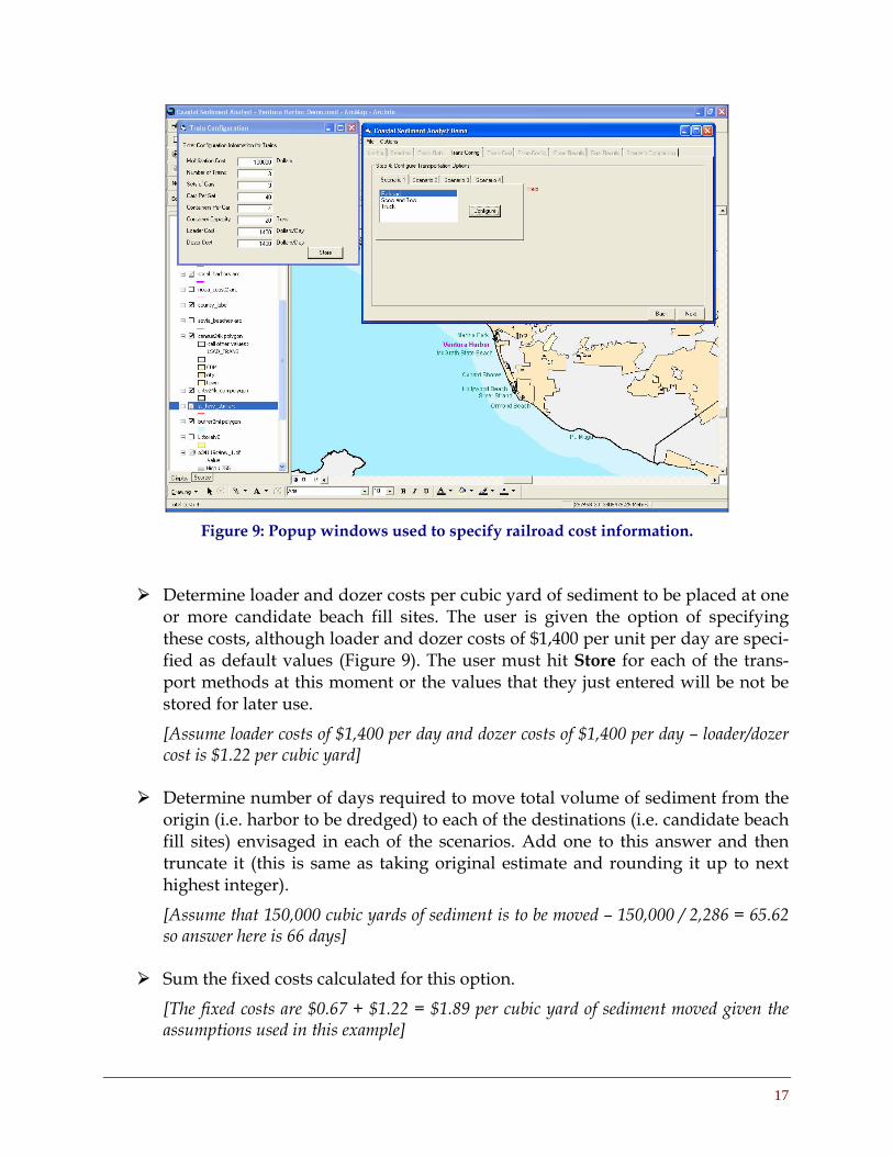
Table 4: Comparison of benefits and costs estimated for Scenario #4 with new Coastal Sedi-ment Analyst and by EIC.

A. CSA Tool

B. EIC (Appendix A)

The benefits of adding additional beach fill to Carpinteria and Oil Piers estimated with the Coastal Sediment Analyst tool were very similar to those reported by EIC (see Ap-pendix A for additional details) for all four scenarios and both the travel cost and tax impact methods. Hence, the three values estimated for Carpinteria Beach in Scenario #1 were within ± 6.8% of those reported by EIC (see Table 1 for additional details) and similar results (differences in the ± 5% range) were produced for the other two scenarios in which this particular beach was included. The benefits calculated for Oxnard Shores with the CSA tool, on the other hand, were 80% (travel cost method) to 100% (tax impact method) higher than those estimated by EIC (see Tables 3 and 4 for details). This discrepancy occurred because of changes made to the estimated number of new visitors and the additional expenditures per visitor pro-jected for this particular beach with a doubling of beach width towards the end of the project. The CSA tool assumes that a doubling of beach width will generate a 20% in-crease in the number of visitors and an 18% increase in the total expenditures per visitor at all of the beaches included in at least one of the scenarios – hence, these rates were applied to every beach in all four scenarios, whereas EIC used these rates for Carpinte-ria and Oil Piers but not Oxnard Shores. The EIC estimates assumed that a doubling of beach width at Oxnard Shores would produce 10% increases in both the number of visi-tors and the total expenditures per visitor. The discrepancies between the two sets of estimates highlight some of the subtleties involved in building these types of tools and

Variable Carpinteria Oil Piers Oxnard Shores Totals Least transportation cost $522,000 $426,000 $313,500 $1,261,500 Recreational benefit (PV) $9,953,077 $202,523 $141,816 $30,582,842 Recreational benefit/cost ratio 19.1 0.5 0.45 24.9 State economic impact (PV) $12,361,540 $177,518 $162,439 $37,101,799 Economic impact/cost ratio 23.7 0.4 0.52 30.2 State tax revenues (PV) $988,923 $14,201 $12,995 $2,968,144 State tax revenue/cost ratio 1.9 0.03 0.04 2.4

Variable Carpinteria Oil Piers Oxnard Shores Totals Least transportation cost $819,000 $690,000 $532,500 $2,041,500 Recreational benefit (PV) $10,940,097 $218,153 $78,975 $11,237,225 Recreational benefit/cost ratio 13.4 0.3 0.1 5.5 State economic impact (PV) $12,373,400 $177,489 $81,303 $12,632,191 Economic impact/cost ratio 15.1 0.3 0.2 6.2 State tax revenues (PV) $989,872 $14,199 $6,504 $1,010,575 State tax revenue/cost ratio 1.2 0.02 0.01 0.5

34

how small changes in parameters can impact the final estimates produced with these types of tools. That said, the Oxnard Shores results did not change the overall results in this particular study because the benefits of adding additional beach fill at Carpinteria far exceeded the benefits of adding beach fill at the other two beach fill sites that were considered. Looking beyond the four scenarios used to develop and test these new tools, there are four sets of limitations and shortcomings that will need to be addressed to facilitate the use of these new tools for analyzing additional harbors and beach fill sites along the California coast and further afar. First, the geospatial datasets displayed in Figures 1 (harbors), 3 (beaches), 6 (railroad network), and 8 (road network) would have to be expanded to cover the entire length of the California coast. Most of these datasets can be compiled from existing public do-main data sources, although some additional work may be required to fix three types of problems. The first task is to check each file for accuracy, completeness, etc. The second is to clip the files to show just the coastal areas because the two transportation files are large and their use for tracing shortest paths on the road and rail networks may cause consider-able delays on networks with large numbers of nodes and/or links. The final task is to add missing information – one node is required for each beach on the railroad network to facilitate the unloading and placement of new sediment at this beach fill site for ex-ample). The drawing tools used in the current version of the Coastal Sediment Analyst to calculate the scow and tow transportation costs could be utilized to draw additional road and railway lines closer to the candidate beaches with some additional program-ming in subsequent versions as well. Second, some additional data and/or functions describing the historical dredging pat-terns at other harbors and the sediment budgets at specific beaches would need to be compiled and (preferably) accessed by the Coastal Sediment Analyst tool from one or more database files. These data would include estimates of current beach width and some knowledge about how beach width might be expected to change over time with and without the placement of varying volumes of new sediment (i.e. beach fill). The best solution here might involve the development of various functions and/or graphs for estimating one or more of these variables from readily available and/or easily ob-tained data inputs. It might be possible to utilize the aerial photographic survey of the California Coast that is updated on a periodic basis as a part of the California Coastal Records Project to help with the development and maintenance of these types of data inputs for example (see Adelman (2004) for additional details). The third set of changes is the least arduous and involves the specification of unit costs for the two additional dredging and conveyance methods – hydraulic pipeline and

35

hopper dredge and pumpout – included in the current prototype. These default values should be included in the CSA toolbox (similar to what happens now for the three op-tions included in the current prototype). The fourth and final set of limitations and shortcomings concerns the recreational use of the various beaches. Ideally, the final tools would work best if some additional data and/or functions describing the current numbers of beach visitors and their spending behavior and how these attributes could be expected to change with changes in beach width over time at specific beaches were compiled and accessed by the CSA tool from one or more database files. The specification of this information for the three candidate beach fill sites used for the current application involved considerable work. These vari-ables may be the most difficult to compile and use at the desired level of granularity for the type of application that was envisaged when this project was started.

36

This page intentionally left blank

37

Conclusions The Coastal Sediment Analyst tool described in the previous sections was written in Visual Basic and applied to the same harbor and beach fill sites used by EIC to prepare Appendix A. The current prototype incorporates a single user interface, an elaborate series of on-line help documents, and various error catching routines. This new tool produced similar cost results to those generated by EIC – there were small differences because the new tool calculated the railroad, scow and tow, and truck distances from the underlying geospatial datasets and these lengths were slightly different than those used by EIC in Appendix A and/or because of different assumptions used to estimate project mobilization/demobilization costs when two or more candidate beach sites were considered. Similar benefits were also calculated with the new CSA tool for two of the three beaches considered. The higher benefits estimated for Oxnard Shores occurred because EIC used lower estimates than the CSA tool for the increases in the number of visitors and total expenditures per visitor that would accompany the doubling of beach width at this particular beach site. Given the aforementioned results and characteristics, the new prototype satisfies the design and performance criteria that were specified at the start of the project. However, there are at least four sets of limitations and shortcomings with the current prototype that would need to addressed in order to use this type of tool to analyze conditions at other California harbors and/or beaches:

The geospatial datasets describing the harbors, beaches, railroad network, and road network would need to be expanded to cover the entire California coast.

Some additional data and/or functions describing the historical dredging pat-terns at other harbors and the sediment budgets at specific beaches would need to be compiled and accessed by the Coastal Sediment Analyst tool from a data-base.

The unit costs for the final two additional dredging and conveyance methods in-cluded in the current Coastal Sediment Analyst toolbox would need to be fleshed out and included in the CSA toolbox as defaults as is done now for the other op-tions.

Some additional data and/or functions describing the current numbers of beach visitors and their spending behavior and how these attributes could be expected to change with changes in beach width over time at specific beaches would need to be compiled and accessed by the Coastal Sediment Analyst tool from a data-base.

These limitations and shortcomings would need to be addressed and/or the Coastal Sediment Analyst tools themselves would need to be modified to support the deploy-ment of these new tools and data to address sediment management issues along other parts of the California coast.

38

This page left intentionally blank

39

Literature Cited Adelman, Kenneth. 2004. California Coastal Records Project. WWW document,

http://www.californiacoastline.org/ (last accessed 28 April 2004)

40

This page left intentionally blank