Embed Size (px)
Citation preview
THE BEST AND WORST OF ALL POSSIBLE WORLDS: SOME CRUDE EVALUATIONS
By
Martin Shubik and Michael R. Powers
June 2017
COWLES FOUNDATION DISCUSSION PAPER NO. 2093
COWLES FOUNDATION FOR RESEARCH IN ECONOMICS YALE UNIVERSITY
Box 208281 New Haven, Connecticut 06520-8281
http://cowles.yale.edu/
THE BEST AND WORST OF ALLPOSSIBLE WORLDS:
SOME CRUDE EVALUATONS
Martin Shubik and Michael R. Powers
June 29, 2017
Contents
1 The 2× 2 Matrix Games with Cardinal Payoffs . . . . . . . . . . . . . . . 22 Outcome Sets . . . . . . . . . . . . . . . . . . . . . . . . . . . . . . . . . . 22.1 Fairness and effi ciency . . . . . . . . . . . . . . . . . . . . . . . . . . 2
3 Behavior and Structure . . . . . . . . . . . . . . . . . . . . . . . . . . . . . 33.1 Effi ciency and behavior . . . . . . . . . . . . . . . . . . . . . . . . . . 4
3.1.1 Inference and pure believers . . . . . . . . . . . . . . . . . . . 43.1.2 Some lessons on structure and behavior . . . . . . . . . . . . . 73.1.3 A note on viability and environment . . . . . . . . . . . . . . 8
3.2 Effi ciency Measures in All 2× 2 games . . . . . . . . . . . . . . . . . 93.2.1 Games of coordination: n = 8 . . . . . . . . . . . . . . . . . . 93.2.2 Mixed motive games 1: n = 7 . . . . . . . . . . . . . . . . . . 93.2.3 Mixed motive games 2: n = 6 . . . . . . . . . . . . . . . . . . 103.2.4 Games of pure opposition: n = 5 . . . . . . . . . . . . . . . . 103.2.5 All mixed motive games: Index2 . . . . . . . . . . . . . . . . . 103.2.6 Fools matter . . . . . . . . . . . . . . . . . . . . . . . . . . . . 113.2.7 Being Nice matters in context . . . . . . . . . . . . . . . . . . 11
4 Costs, Coordination and Cooperation . . . . . . . . . . . . . . . . . . . . 115 References . . . . . . . . . . . . . . . . . . . . . . . . . . . . . . . . . . . . 126 Appendix 1 Indices . . . . . . . . . . . . . . . . . . . . . . . . . . . . . . . 137 Appendix 2: 144 games . . . . . . . . . . . . . . . . . . . . . . . . . . . . . . . . . . . . . . . . . 17
Abstract
The 2 × 2 matrix game plays a central role in the teaching and expositionof game theory. It is also the source of much experimentation and researchin political science, social psychology, biology and other disciplines. This briefpaper is addressed to answering one intuitively simple question without going
1
into the many subtle qualifications that are there. How effi cient is the non-cooperative equilibrium? This is part of a series of several papers that addressmany of the qualifications concerning the uses of the 2 X 2 matrix games.JEL Classifications: C63, C72, D61Keywords: 2×2 matrix games, index,
1 The 2× 2 Matrix Games with Cardinal PayoffsIn the folklore and elementary education of game theory the 2× 2 matrix game hasplayed a special role. Several of these games bear special names such as The Prisoner’sDilemma, The Stag Hunt, and the Battle of the Sexes. There are only 144 strategicallydifferent 2 × 2 games with strictly ordinal preferences. We are often interested inconsidering related games with cardinal preferences and a moment’s considerationshows that there is an indefinite number of these games. Many applications makeit desirable to examine a large but finite set of 2× 2 games with specific numbers ofhighly different sizes. In a different paper we suggest how to do this [4]. This paperutilizes all the 144 games listed in Appendix 2 as they serve to give a suffi cientlyexhaustive coverage of all 2 × 2 games to be able to get a feeling for the effi ciencyof noncooperative and some other behaviors without delving into a more refinedapparatus as we do in [11].
2 Outcome Sets
The 2× 2 matrix game with strictly ordinal payoffs may be cardinalized by 4 > 3 >2 > 1 . We may study the strictly ordinal set of games utilizing just the symbols1, 2, 3, 4 1.Two of the top desirable properties of a good society are effi ciency and fairness,
they can only be defined after the assumptions concerning preferences have beenmade.
2.1 Fairness and effi ciency
Fairness cannot be defined before the initial conditions are spelled out. The fullspecification of initial conditions requires the assumptions made about innate prop-erty rights of individuals. Symmetry involves the consideration of intrinsic propertyrights. These are discussed elsewhere[3], [6],[1],[5],. Here we concentrate only oneffi ciency,which amounts to considering how close actual outcomes are to a jointlymaximal payoff.
1or a, b, c, d or any other icons.
2
3 Behavior and Structure
We consider and contrast several other behaviors beyond noncooperative behavior.Metaphorically we consider four player types described as: The individualist; thepessimist; the optimist or idealist; and the know-nothing, zero-intelligence or fool orentropic player.The Entropic Player : The Entropic player is the player that always acts or
chooses a strategy uniformly at random2.MaxMax(P1+P2): The MaxMax Player is the player who always chooses the
strategy for which the maximum social welfare is achieved. Call her MaxMax orthe Utopian Player. she acts as if she will do the right thing and knows the otherwill do so3. The player makes one simple inference about what the the other playerwill do.MaxsMins̄P1: is defensive he assumes the other side is out to damage him. We
may call the playersMaxMin or pessimistic.A Noncooperative Equilibrium player or NEP assumes that she faces a
player motivated like herself. This behavior can be described by two parallel maxi-mizing equations 4.We consider a pair of noncooperative players playing each other and also contrast
their performance with three other pairs of player types playing four specially namedgames, We then consider all 144 games in aggregate and broken into four structuralcategories now noted.We know that in the initial resource distribution we may break all 144 games into
four natural categories
Joint maximum Frequency8 367 606 425 6Table 1
Frequency of maximal wealth
The 36 games with a joint wealth of 8 each can be called ‘Games of coordination’.There is a single cell with value (4, 4) that is a natural point of attraction.The 6 games with joint maximum equal to 5 are games of pure opposition. There
is no potential opportunity for individual gain from collaboration. The games witha joint maximum of 6 or 7 are mixed motive games where gains can be made by
2He is a syntactic agent whose distinguishes structure but is unable to interpret content or thesemantics.
3If there is more than one joint maximum a selection rule is needed.4As is noted in [4] there are several tehnical details that must be considered concerning how to
handle multiple equilibria. We need to obtain higher and lower bounds on eficiency,
3
coordination and collaboration. We note that the modal wealth of the four types is7.
3.1 Effi ciency and behavior
The work presented here on all possible worlds is made under a considerable heapof assumptions with no comment on the trade-offs between effi ciency and symmetry.This problem is considered elsewhere. Furthermore we consider only ‘pure popula-tions’where agents are matched only against agents of the same type. Except forone illustrative example, players of different types being matched against each otherare considered elsewhere [?], [12]. The mixed, more complex approach is congenialwith evolutionary game theory[2].5
3.1.1 Inference and pure believers
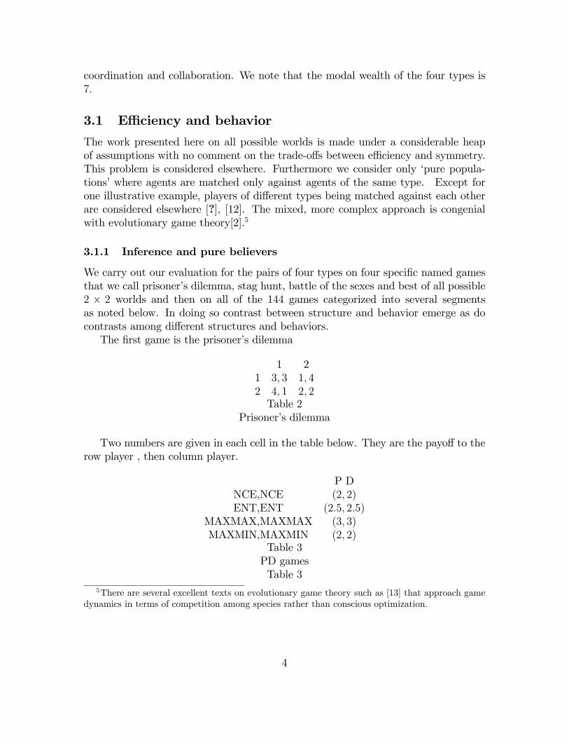
We carry out our evaluation for the pairs of four types on four specific named gamesthat we call prisoner’s dilemma, stag hunt, battle of the sexes and best of all possible2 × 2 worlds and then on all of the 144 games categorized into several segmentsas noted below. In doing so contrast between structure and behavior emerge as docontrasts among different structures and behaviors.The first game is the prisoner’s dilemma
1 21 3, 3 1, 42 4, 1 2, 2Table 2
Prisoner’s dilemma
Two numbers are given in each cell in the table below. They are the payoff to therow player , then column player.
P DNCE,NCE (2, 2)ENT,ENT (2.5, 2.5)
MAXMAX,MAXMAX (3, 3)MAXMIN,MAXMIN (2, 2)
Table 3PD gamesTable 3
5There are several excellent texts on evolutionary game theory such as [13] that approach gamedynamics in terms of competition among species rather than conscious optimization.
4
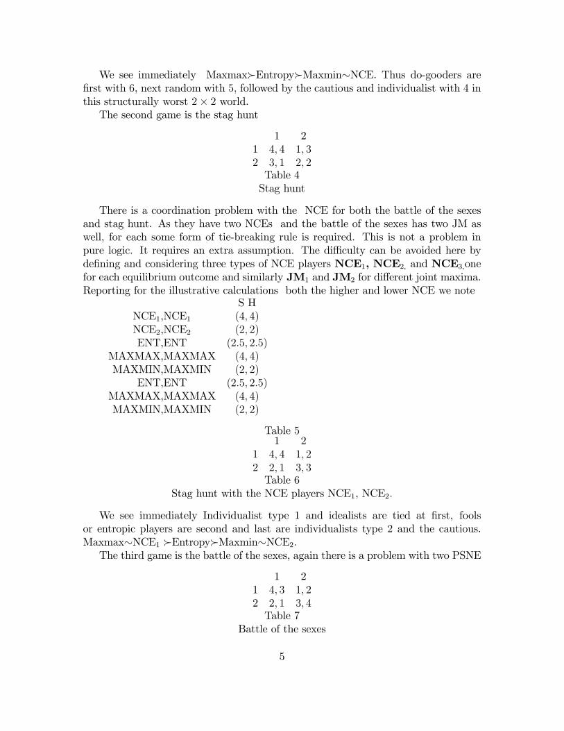
We see immediately Maxmax�Entropy�Maxmin∼NCE. Thus do-gooders arefirst with 6, next random with 5, followed by the cautious and individualist with 4 inthis structurally worst 2× 2 world.The second game is the stag hunt
1 21 4, 4 1, 32 3, 1 2, 2Table 4Stag hunt
There is a coordination problem with the NCE for both the battle of the sexesand stag hunt. As they have two NCEs and the battle of the sexes has two JM aswell, for each some form of tie-breaking rule is required. This is not a problem inpure logic. It requires an extra assumption. The diffi culty can be avoided here bydefining and considering three types of NCE players NCE1, NCE2, and NCE3,onefor each equilibrium outcome and similarly JM1 and JM2 for different joint maxima.Reporting for the illustrative calculations both the higher and lower NCE we note
S HNCE1,NCE1 (4, 4)NCE2,NCE2 (2, 2)ENT,ENT (2.5, 2.5)
MAXMAX,MAXMAX (4, 4)MAXMIN,MAXMIN (2, 2)
ENT,ENT (2.5, 2.5)MAXMAX,MAXMAX (4, 4)MAXMIN,MAXMIN (2, 2)
Table 51 2
1 4, 4 1, 22 2, 1 3, 3Table 6
Stag hunt with the NCE players NCE1, NCE2.
We see immediately Individualist type 1 and idealists are tied at first, foolsor entropic players are second and last are individualists type 2 and the cautious.Maxmax∼NCE1 �Entropy�Maxmin∼NCE2.The third game is the battle of the sexes, again there is a problem with two PSNE
1 21 4, 3 1, 22 2, 1 3, 4Table 7
Battle of the sexes
5
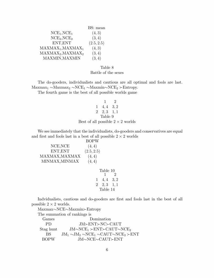
BS: meanNCE1,NCE1 (4, 3)NCE2,NCE2 (3, 4)ENT,ENT (2.5, 2.5)
MAXMAX1,MAXMAX1 (4, 3)MAXMAX2,MAXMAX2 (3, 4)MAXMIN,MAXMIN (3, 4)
Table 8Battle of the sexes
The do-gooders, individualists and cautious are all optimal and fools are last.Maxmax1 ∼Maxmax2 ∼NCE1 ∼Maxmin∼NCE2 �Entropy.The fourth game is the best of all possible worlds game
1 21 4, 4 3, 22 2, 3 1, 1Table 9
Best of all possible 2× 2 worlds
We see immediately that the individualists, do-gooders and conservatives are equaland first and fools last in a best of all possible 2× 2 worlds
BOPWNCE,NCE (4, 4)ENT,ENT (2.5, 2.5)
MAXMAX,MAXMAX (4, 4)MINMAX,MINMAX (4, 4)
Table 101 2
1 4, 4 3, 22 2, 3 1, 1Table 14
Indvidualists, cautious and do-gooders are first and fools last in the best of allpossible 2× 2 worlds.Maxmax∼NCE∼Maxmin�EntropyThe summation of rankings isGames DominationPD JM�ENT�NC�CAUT
Stag hunt JM∼NCE1 �ENT�CAUT∼NCE2
BS JM1 ∼JM2 ∼NCE1 ∼CAUT∼NCE2 �ENTBOPW JM∼NCE∼CAUT�ENT
6
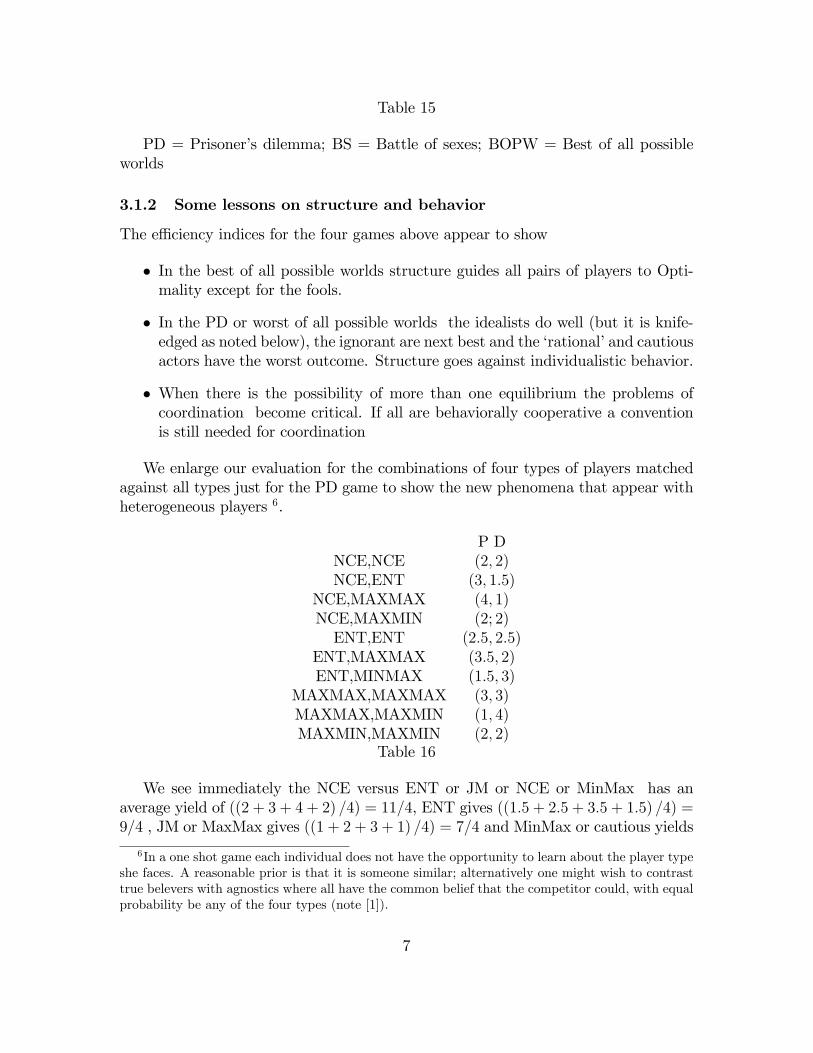
Table 15
PD = Prisoner’s dilemma; BS = Battle of sexes; BOPW = Best of all possibleworlds
3.1.2 Some lessons on structure and behavior
The effi ciency indices for the four games above appear to show
• In the best of all possible worlds structure guides all pairs of players to Opti-mality except for the fools.
• In the PD or worst of all possible worlds the idealists do well (but it is knife-edged as noted below), the ignorant are next best and the ‘rational’and cautiousactors have the worst outcome. Structure goes against individualistic behavior.
• When there is the possibility of more than one equilibrium the problems ofcoordination become critical. If all are behaviorally cooperative a conventionis still needed for coordination
We enlarge our evaluation for the combinations of four types of players matchedagainst all types just for the PD game to show the new phenomena that appear withheterogeneous players 6.
P DNCE,NCE (2, 2)NCE,ENT (3, 1.5)
NCE,MAXMAX (4, 1)NCE,MAXMIN (2; 2)ENT,ENT (2.5, 2.5)
ENT,MAXMAX (3.5, 2)ENT,MINMAX (1.5, 3)
MAXMAX,MAXMAX (3, 3)MAXMAX,MAXMIN (1, 4)MAXMIN,MAXMIN (2, 2)
Table 16
We see immediately the NCE versus ENT or JM or NCE or MinMax has anaverage yield of ((2 + 3 + 4 + 2) /4) = 11/4, ENT gives ((1.5 + 2.5 + 3.5 + 1.5) /4) =9/4 , JM or MaxMax gives ((1 + 2 + 3 + 1) /4) = 7/4 and MinMax or cautious yields
6In a one shot game each individual does not have the opportunity to learn about the player typeshe faces. A reasonable prior is that it is someone similar; alternatively one might wish to contrasttrue belevers with agnostics where all have the common belief that the competitor could, with equalprobability be any of the four types (note [1]).
7
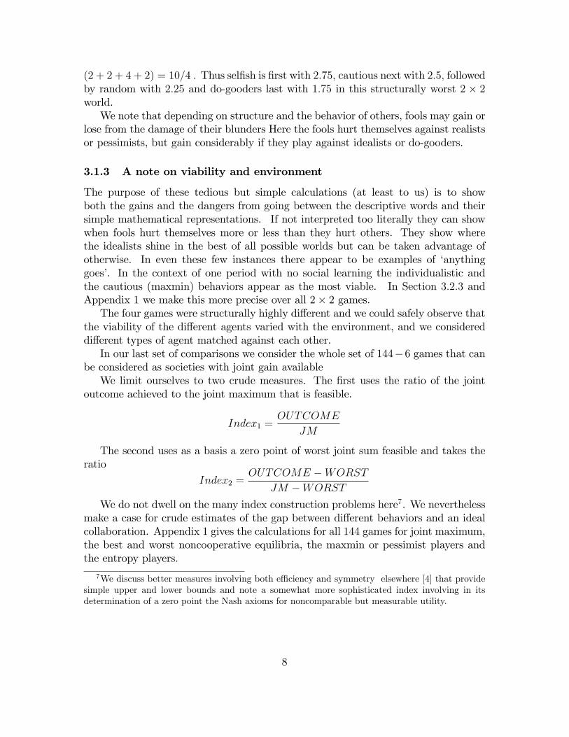
(2 + 2 + 4 + 2) = 10/4 . Thus selfish is first with 2.75, cautious next with 2.5, followedby random with 2.25 and do-gooders last with 1.75 in this structurally worst 2 × 2world.We note that depending on structure and the behavior of others, fools may gain or
lose from the damage of their blunders Here the fools hurt themselves against realistsor pessimists, but gain considerably if they play against idealists or do-gooders.
3.1.3 A note on viability and environment
The purpose of these tedious but simple calculations (at least to us) is to showboth the gains and the dangers from going between the descriptive words and theirsimple mathematical representations. If not interpreted too literally they can showwhen fools hurt themselves more or less than they hurt others. They show wherethe idealists shine in the best of all possible worlds but can be taken advantage ofotherwise. In even these few instances there appear to be examples of ‘anythinggoes’. In the context of one period with no social learning the individualistic andthe cautious (maxmin) behaviors appear as the most viable. In Section 3.2.3 andAppendix 1 we make this more precise over all 2× 2 games.The four games were structurally highly different and we could safely observe that
the viability of the different agents varied with the environment, and we considereddifferent types of agent matched against each other.In our last set of comparisons we consider the whole set of 144−6 games that can
be considered as societies with joint gain availableWe limit ourselves to two crude measures. The first uses the ratio of the joint
outcome achieved to the joint maximum that is feasible.
Index1 =OUTCOME
JM
The second uses as a basis a zero point of worst joint sum feasible and takes theratio
Index2 =OUTCOME −WORST
JM −WORSTWe do not dwell on the many index construction problems here7. We nevertheless
make a case for crude estimates of the gap between different behaviors and an idealcollaboration. Appendix 1 gives the calculations for all 144 games for joint maximum,the best and worst noncooperative equilibria, the maxmin or pessimist players andthe entropy players.
7We discuss better measures involving both effi ciency and symmetry elsewhere [4] that providesimple upper and lower bounds and note a somewhat more sophisticated index involving in itsdetermination of a zero point the Nash axioms for noncomparable but measurable utility.
8
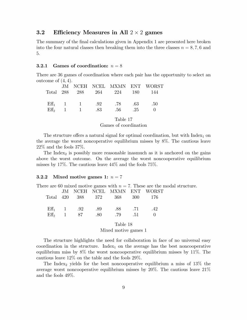
3.2 Effi ciency Measures in All 2× 2 gamesThe summary of the final calculations given in Appendix 1 are presented here brokeninto the four natural classes then breaking them into the three classes n = 8, 7, 6 and5.
3.2.1 Games of coordination: n = 8
There are 36 games of coordination where each pair has the opportunity to select anoutcome of (4, 4).
JM NCEH NCEL MXMN ENT WORSTTotal 288 288 264 224 180 144
Eff1 1 1 .92 .78 .63 .50Eff2 1 1 .83 .56 .25 0
Table 17Games of coordination
The structure offers a natural signal for optimal coordination, but with Index1 onthe average the worst noncoperative equilibrium misses by 8%. The cautious leave22% and the fools 37%.The Index2 is possibly more reasonable inasmuch as it is anchored on the gains
above the worst outcome. On the average the worst noncooperative equilibriummisses by 17%. The cautious leave 44% and the fools 75%.
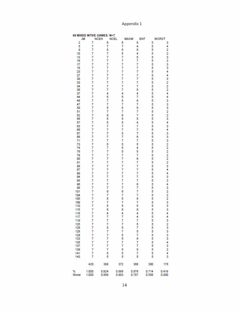
3.2.2 Mixed motive games 1: n = 7
There are 60 mixed motive games with n = 7. These are the modal structure.JM NCEH NCEL MXMN ENT WORST
Total 420 388 372 368 300 176
Eff1 1 .92 .89 .88 .71 .42Eff2 1 87 .80 .79 .51 0
Table 18Mixed motive games 1
The structure highlights the need for collaboration in face of no universal easycoordination in the structure. Index1 on the average has the best noncooperativeequilibrium miss by 8% the worst noncooperative equilibrium misses by 11%. Thecautious leave 12% on the table and the fools 29%.The Index2 yields for the best noncooperative equilibrium a miss of 13% the
average worst noncooperative equilibrium misses by 20%. The cautious leave 21%and the fools 49%.
9

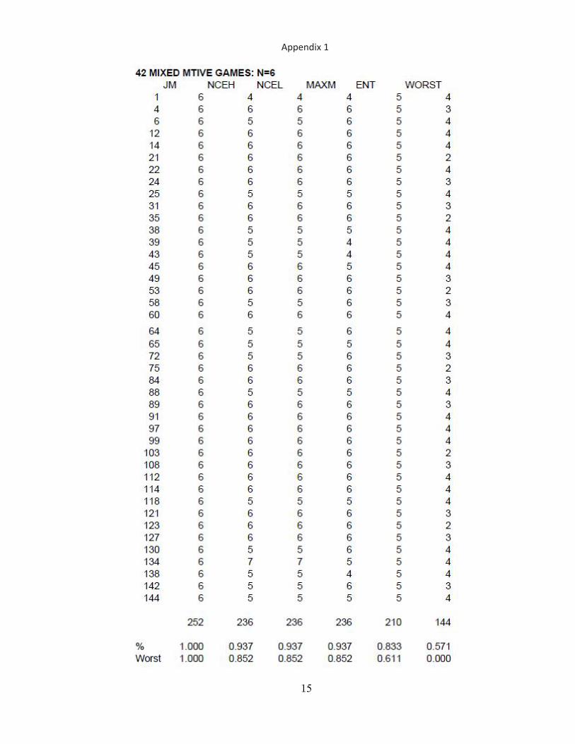
3.2.3 Mixed motive games 2: n = 6
There are 42 mixed motive games with n = 6. They have less fat to fight over thanthose previously noted.
JM NCEH NCEL MXMN ENT WORSTTotal 252 236 236 236 210 144
Eff1 1 .94 .94 .94 .83 .57Eff2 1 .85 .85 .85 .61 0
Table 19Mixed motive games 2
Index1 on the average has the best noncooperative equilibrium, the worst non-cooperative equilibrium and the cautious all leave 7% on the table and the fools17%.The Index2 yields the same for best noncooperative equilibrium worst nonco-operative equilibrium and the cautious all leave 15% and the fools 39%
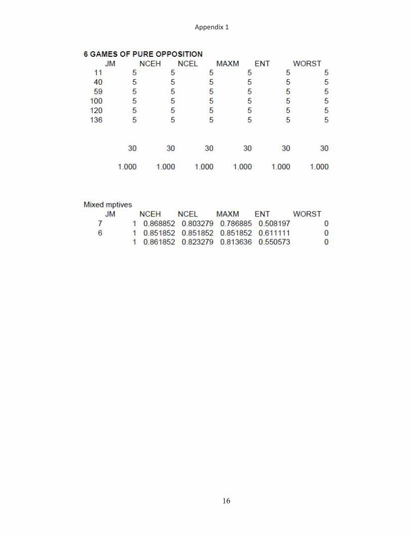
3.2.4 Games of pure opposition: n = 5
There are only 6 mixed motive games with n = 5. They have a pure opposition ofinterests as is noted in Table 20
JM NCEH NCEL MXMN ENT WORSTTotal 30 30 30 30 30 30
Eff1 1 1 1 1 1 1Eff2 1 1 1 1 1 1
Table 20
Paradoxically the handful of constant sum games with a joint maximum of 5 haveevery outcome as Pareto optimal thus to include them in a measure primarily aimedat considering joint gains in a society is misleading. The intent operators NCE,MaxMax, Maxmin all collapse to yielding the same behavior in a two personHobbsian constant sum world.
3.2.5 All mixed motive games: Index2
Table 21 displays the values of the second index over all games with mixed motivesJM NCEH NCEL MXMN ENT WORST
n=7 1 .87 .8 .79 .51 0n=6 1 .85 .85 .85 .61 0
1 .86 .82 .81 .55 0
Table 21
10
The bounds on the average effi ciency of purely individualistic behavior appear tobe between at least 14% and at most 18% with purely defensive behavior coming inclose at 19%
3.2.6 Fools matter
Looking over the various games and solutions damage done by the ignorant varies.We may regard all non learning purely syntactic players as being societally tone deaf.The other players may or may not be concerned with how much the ignorant
damage themselves, but it is easy to produce games where the fools damage othersas well as themselves. The clever game theorist, can easily cook up examples whereit pays the cunning to play the fool, but often fools are fools.
3.2.7 Being Nice matters in context
In various outcomes here always being intrinsically cooperative does not pay. Whenthe structure is as the best of all possible worlds joint maximality is coaxed out of allsyntactic,non-malicious player types modeled here.In philosophical writings we have the realism and skepticism of Hobbes and
Voltaire contrasting with the fuzzy-headedness mythology of the original perfectprimitive world of the trendy salon speaker Rousseau. The more realistic view ap-pears to be that of Hume where the social individual is cooperative but no fool. Inorder to start to do justice to such a player we would need at least two plays wherelearning can begin. It is here where a tit-for-tat player can be considered. The oneply does not permit flexibility but the two ply opens up a manageable set of minimallearning possibilities
4 Costs, Coordination and Cooperation
• Civilization, culture, society and law move on broader and slower time scalesthan everyday life and almost all of the individual consumer and worker eco-nomic and political activities.
• Effi ciency and symmetry are critical features of everyday life.
• The construction of indices are critical for the measurements of deviations fromeffi ciency and symmetric treatment of individuals
• Threats play a key role in considering what the zero point should be on anyindex understanding the implications of comparable utility is merited first.
We do not live in the utopian best of all possible worlds and do not live in purelydystopian structures. We have rich or not so rich mixed motive structures. The
11
models of the noncooperative and cautious or pessimistic agents are metaphors fordecentralized behavior. But the behavior is within the structure of the rules of thegame. The departure from Optimality appears to range from a low of around 15to 20% that can be considered as the potential gain available from coordination andcooperation.
5 References
References
[1] Harsanyi, J. C. 1963. A simplified bargaining model for the n-person cooperativegame. International Economic Review 4:194—220.
[2] Maynard Smith, J. 1982 Evolution and the Theory of Games Cambridge: Cam-bridge University Press.
[3] Nash, J. F. 1953. Two-person cooperative games. Econometrica 21 (1):128—140.
[4] Powers, M. and M. Shubik. The value of government. Manuscript in preparation.
[5] J.A. Rawls 1971Theory of Justice Belknap, Cambridge
[6] Shapley, L. S. A value for n-person games in: H. Kuhn, A.W. Tucker (Eds.), Con-tributions to the Theory of Games, vol. 2, Princeton University Press, Princeton,NJ (1953), pp. 307—317
[7] Shubik, M. 2008.A note on fairness, power, property and behind the veil. Eco-nomics Letters 98, 1: 29—30
[8] Shubik,M. “A Web Gaming Facility for Research and Teaching” (May 2012)CFDP 1860 and “What Is a Solution to a Matrix Game” (July 2012) CFDP1866.
[9] Shubik, M., J. Faber, D. Li. The many worlds of the 2 × 2 games with heterogeneous
[10] Shubik, M and E. Smith 2016 The Guidance of a Enterprise Economy (with DEric Smith) Cambridge, MA; UK: MIT Press,
[11] Shubik M, G. .Powers and Wen
[12] Shubik M, G. .Powers
[13] Weibull J. 1995 Evolutionary Game Theory Cambridge, MA: M.I.T. Press: ISBN0-262-23181-6; Paper: ISBN 0-262-73121-5
12
agents. Manuscript in preparation.
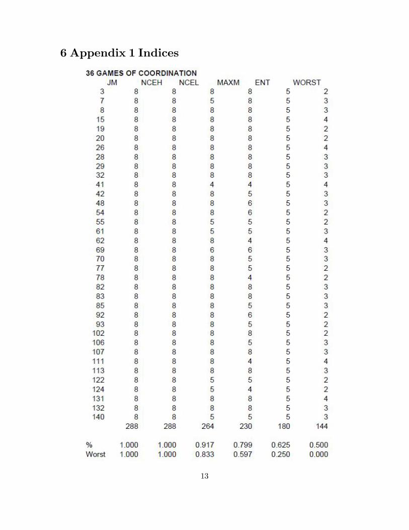
6 Appendix 1 Indices
13
14
Appendix 1
15
Appendix 1
16
Appendix 1
Row Col.(1,4) (3,3)
(2,2) (4,1)
(1,2) (3,1)
(2,4) (4,3)
(1,1) (3,2)
(2,3) (4,4)
(1,4) (3,3)
(4,2) (2,1)
(1,3) (3,4)
(4,1) (2,2)
(1,3) (3,2)
(4,1) (2,4)
(1,2) (3,3) 4 4
(4,4) (2,1) 3 3
(1,2) (3,1)
(4,4) (2,3)
(1,1) (3,2)
(4,3) (2,4)
(1,1) (3,4) 3 4
(4,3) (2,2) 4 3
(1,4) (2,3)
(3,2) (4,1)
(1,4) (2,2)
(3,3) (4,1)
(1,4) (2,1)
(3,2) (4,3)
(1,3) (2,4)
(3,1) (4,2)
(1,3) (2,2)
(3,1) (4,4)
(1,2) (2,3)
(3,4) (4,1)
(1,2) (2,4)
(3,1) (4,3)
(1,2) (2,1)
(3,4) (4,3)
(1,1) (2,3)
(3,2) (4,4)
(1,1) (2,2)
(3,3) (4,4)
(1,1) (2,4)
(3,3) (4,2)
(1,4) (2,3)
(4,2) (3,1)
Game # Symmetric
Sym
Sym
Sym
Sym
Sym
Sym
137
86
109
NA
102
123
114
Transpose
22 NA
115
NA
108
117
134
NA
113
105
NA
120
NA
128
112
131
Shape
20
16
18
7
9
5
2
24
22
19
17
15
10
11
8
3
1
Dom.ParetoOptima
1 6 1
JointMax
PSNEsNash PayoffPayoff
Matrix
2 13 8 1 4 4
2 2 2 3
2 711
3
3 3 2 312 6 1
7 8 2
0 210 7 2
2.5 2.5 0 36 6 0
0 1
16 7 1 3 4 1
4 2 2
15 8
4 1 25 7 1 3
1 2 4 2 2
1 3
1 4
1 4 4 1 18 8
21 6
20 8 1 4 4 2
4 1 1
2
18 7
1 3 3 1 36
23
4 6
2 1 29 7 1 3
1 4 2 1 3
17 7 1 4 3
11 5 1 3 2 2
14 6 1 4
1 4 3 1 2
4
13 7
2
22 6
2
2 2 2
1
1 4 2 2 3
1 4 4 2 119 8
17
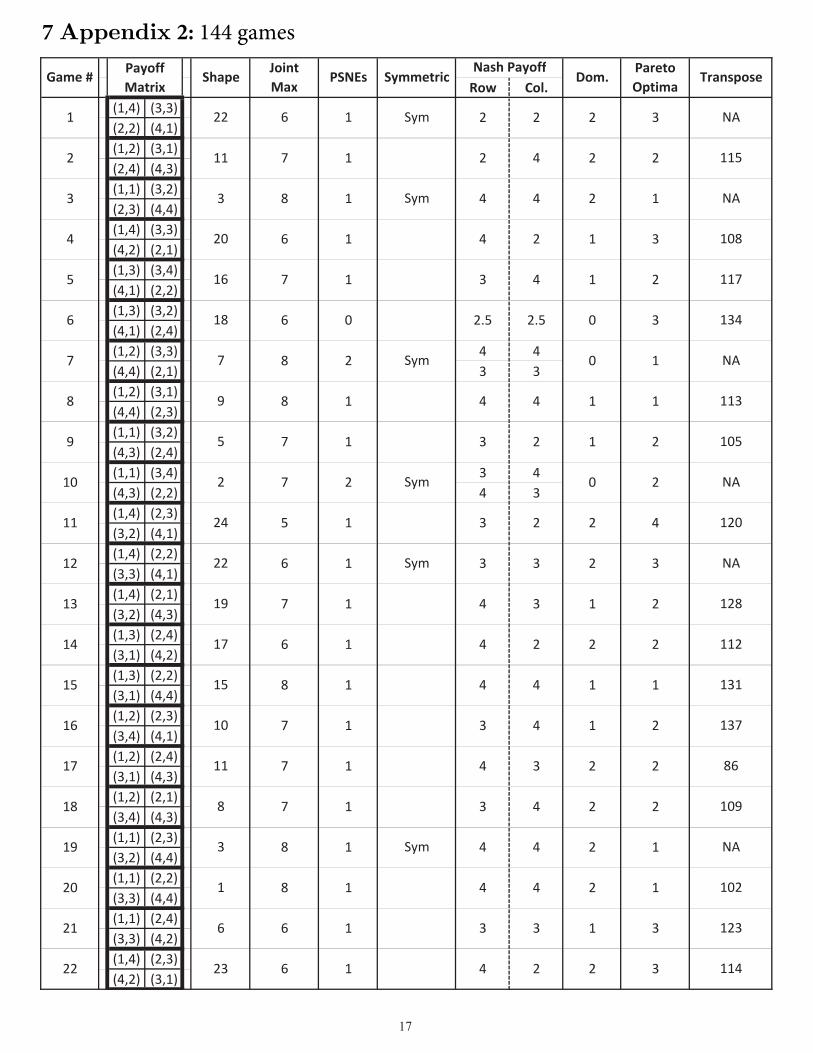
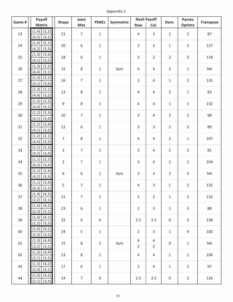
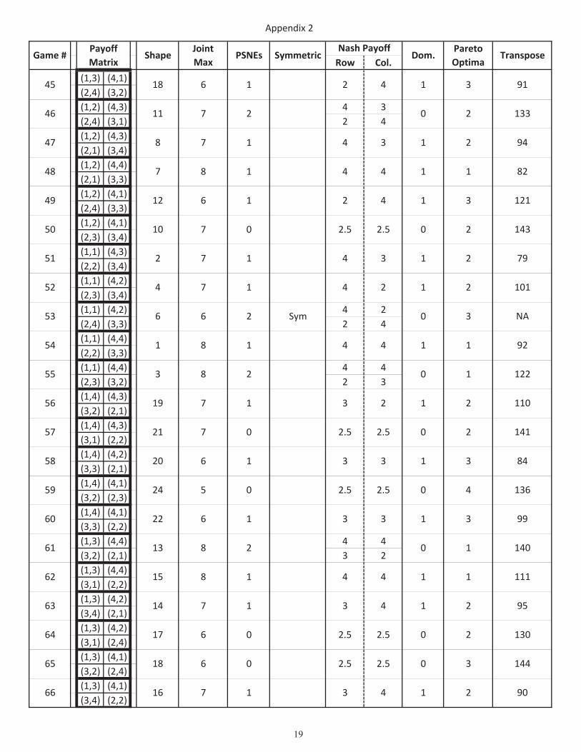
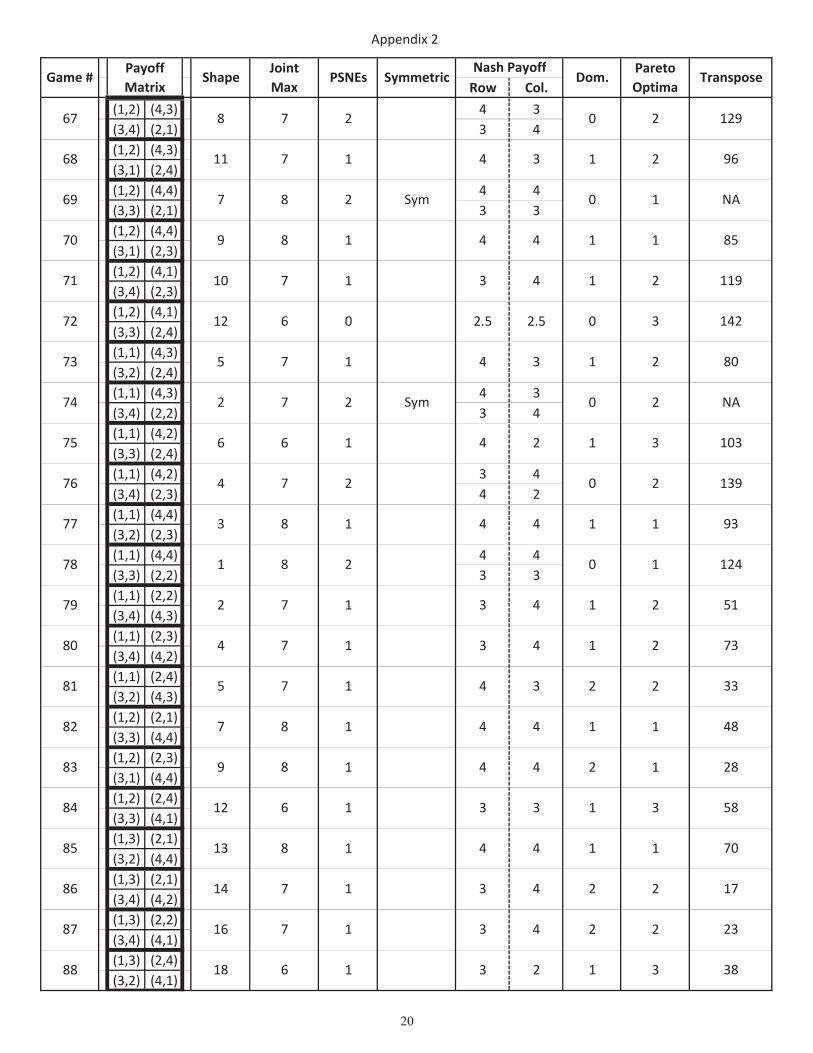
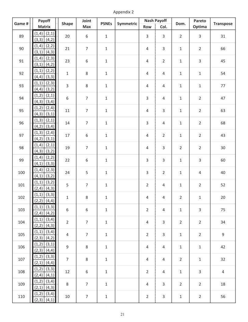
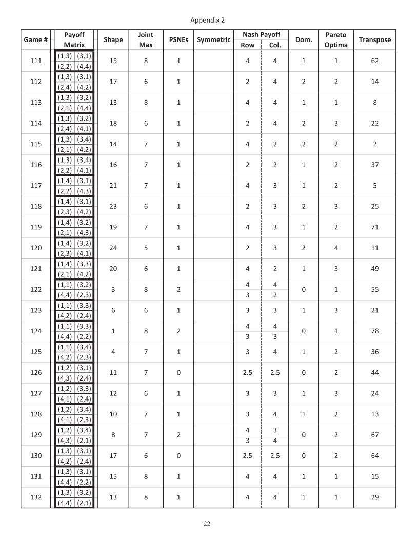
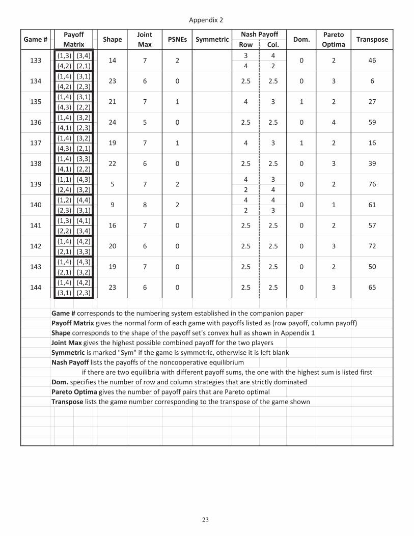
7 Appendix 2: 144 games
Appendix 2
Row Col.Game # Symmetric TransposeShape Dom.
ParetoOptima
JointMax
PSNEsNash PayoffPayoff
Matrix
(1,4) (2,2)
(4,3) (3,1)
(1,4) (2,1)
(4,2) (3,3)
(1,3) (2,4)
(4,1) (3,2)
(1,3) (2,2)
(4,4) (3,1)
(1,3) (2,2)
(4,1) (3,4)
(1,3) (2,1)
(4,4) (3,2)
(1,2) (2,3)
(4,4) (3,1)
(1,2) (2,3)
(4,1) (3,4)
(1,2) (2,4)
(4,1) (3,3)
(1,2) (2,1)
(4,4) (3,3)
(1,1) (2,3)
(4,2) (3,4)
(1,1) (2,2)
(4,3) (3,4)
(1,1) (2,4)
(4,2) (3,3)
(1,1) (2,4)
(4,3) (3,2)
(1,4) (4,3)
(2,2) (3,1)
(1,4) (4,2)
(2,3) (3,1)
(1,4) (4,1)
(2,2) (3,3)
(1,4) (4,1)
(2,3) (3,2)
(1,3) (4,4) 4 4
(2,2) (3,1) 2 2
(1,3) (4,4)
(2,1) (3,2)
(1,3) (4,2)
(2,4) (3,1)
(1,3) (4,2)
(2,1) (3,4)
Sym
Sym
81
104
NA
125
116
88
138
100
NA
106
97
126
87
127
118
NA
135
83
132
98
89
107
24
15
13
17
14
21
20
18
15
16
13
9
10
12
7
3
2
6
5
21
23
22
Sym
0 141 8 2
43 6 1 2
0 339 6 0 2.5 2.5
2 3
2.5 2.5 0 244 7 0
7
1 2 2
3
30 7 1 3 4 2
4 1 227 7 1 3
1 2
1
4 2 234 7 1 3
1 3 4 2 233 7
1 2
1 4 3 1 236
28 8 1 4 4 2
1 324 6 1 3
31 6 1 3
1 4 4 1 1
1
29 8
2
2 126 8 1 4
3 2 3
4 1 142 8 1 4
1 2 3 1 4
3
40 5
38
1
37 7
32 8 1 4 4 2
6 1
4
25 6 1 3 2 2
3 2 223 7 1 4
3
3
35 6 1 3 3 2
4
18
Appendix 2
Row Col.Game # Symmetric TransposeShape Dom.
ParetoOptima
JointMax
PSNEsNash PayoffPayoff
Matrix
(1,3) (4,1)
(2,4) (3,2)
(1,2) (4,3) 4 3
(2,4) (3,1) 2 4
(1,2) (4,3)
(2,1) (3,4)
(1,2) (4,4)
(2,1) (3,3)
(1,2) (4,1)
(2,4) (3,3)
(1,2) (4,1)
(2,3) (3,4)
(1,1) (4,3)
(2,2) (3,4)
(1,1) (4,2)
(2,3) (3,4)
(1,1) (4,2) 4 2
(2,4) (3,3) 2 4
(1,1) (4,4)
(2,2) (3,3)
(1,1) (4,4) 4 4
(2,3) (3,2) 2 3
(1,4) (4,3)
(3,2) (2,1)
(1,4) (4,3)
(3,1) (2,2)
(1,4) (4,2)
(3,3) (2,1)
(1,4) (4,1)
(3,2) (2,3)
(1,4) (4,1)
(3,3) (2,2)
(1,3) (4,4) 4 4
(3,2) (2,1) 3 2
(1,3) (4,4)
(3,1) (2,2)
(1,3) (4,2)
(3,4) (2,1)
(1,3) (4,2)
(3,1) (2,4)
(1,3) (4,1)
(3,2) (2,4)
(1,3) (4,1)
(3,4) (2,2)
143
79
101
NA
92
122
110
141
84
136
99
140
111
95
130
144
90
91
133
94
82
121
18
11
8
7
12
10
2
4
6
1
3
19
0 161 8 2
0 264 6 0
66 7 1
13
15
14
17
18
16 3 4
8 2
0 246 7 2
21
20
24
22
Sym
0
0 250 7 0 2.5 2.5
0 3
2
52 7
51 7 1 4 3 1
53 6 2
0 155
0 459 5 0 2.5 2.5
2.5 2.5 0 257
65 6
7
3 1 2
1
2
4 1 263 7 1 3
0 30 2.5
1
54 8
48 8 1 4 4 1
1
47 7 1 4
6 1 3
1 4 4 1 1
4 1 3
3
49 6
45 6 1 2 4 1
2.5
2.5 2.5
60 6 1 3 3 1
3 1 358
1 4 4 1 1
3
62 8
2
2 1 256 7 1 3
1 4 2 1 2
19
Appendix 2
Row Col.Game # Symmetric TransposeShape Dom.
ParetoOptima
JointMax
PSNEsNash PayoffPayoff
Matrix
(1,2) (4,3) 4 3
(3,4) (2,1) 3 4
(1,2) (4,3)
(3,1) (2,4)
(1,2) (4,4) 4 4
(3,3) (2,1) 3 3
(1,2) (4,4)
(3,1) (2,3)
(1,2) (4,1)
(3,4) (2,3)
(1,2) (4,1)
(3,3) (2,4)
(1,1) (4,3)
(3,2) (2,4)
(1,1) (4,3) 4 3
(3,4) (2,2) 3 4
(1,1) (4,2)
(3,3) (2,4)
(1,1) (4,2) 3 4
(3,4) (2,3) 4 2
(1,1) (4,4)
(3,2) (2,3)
(1,1) (4,4) 4 4
(3,3) (2,2) 3 3
(1,1) (2,2)
(3,4) (4,3)
(1,1) (2,3)
(3,4) (4,2)
(1,1) (2,4)
(3,2) (4,3)
(1,2) (2,1)
(3,3) (4,4)
(1,2) (2,3)
(3,1) (4,4)
(1,2) (2,4)
(3,3) (4,1)
(1,3) (2,1)
(3,2) (4,4)
(1,3) (2,1)
(3,4) (4,2)
(1,3) (2,2)
(3,4) (4,1)
(1,3) (2,4)
(3,2) (4,1)
Sym
Sym
58
70
17
23
38
129
96
NA
85
119
142
80
NA
103
139
93
124
51
73
33
48
28
16
7 2
0 178 8 2
87 7 1 3
1 3 4 2 2
18
0 267 7 2
71 7
8
11
7
9
0 169 8 2
2.5 2.5 0 372 6 0
0 2
80 7 1 3 4 1
4 1 279 7 1 3
1 3 4 1 2
2
1
10
12
5
2
6
4
3
1
2
4
5
7
9
12
13
1486 7
4 2 2
8 4
3
85 8
68 7 1 4 3 1 2
77 8 1 4 4 1
4 1 170
3 2 281 7 1 4
1 4 3 1 273 7
1
83 8 1 4
1 4 4 1 182 8
76
0 274 7 2
388 6 1 3 2 1
1 4 4 1 1
84 6 1 3 3 1
4 2 1
375 6 1 4 2 1
20
Appendix 2
Row Col.Game # Symmetric TransposeShape Dom.
ParetoOptima
JointMax
PSNEsNash PayoffPayoff
Matrix
(1,4) (2,1)
(3,3) (4,2)
(1,4) (2,2)
(3,1) (4,3)
(1,4) (2,3)
(3,1) (4,2)
(1,1) (2,2)
(4,4) (3,3)
(1,1) (2,3)
(4,4) (3,2)
(1,2) (2,1)
(4,3) (3,4)
(1,2) (2,4)
(4,3) (3,1)
(1,3) (2,1)
(4,2) (3,4)
(1,3) (2,4)
(4,2) (3,1)
(1,4) (2,1)
(4,3) (3,2)
(1,4) (2,2)
(4,1) (3,3)
(1,4) (2,3)
(4,1) (3,2)
(1,1) (3,2)
(2,4) (4,3)
(1,1) (3,3)
(2,2) (4,4)
(1,1) (3,3)
(2,4) (4,2)
(1,1) (3,4)
(2,2) (4,3)
(1,1) (3,4)
(2,3) (4,2)
(1,2) (3,1)
(2,3) (4,4)
(1,2) (3,3)
(2,1) (4,4)
(1,2) (3,3)
(2,4) (4,1)
(1,2) (3,4)
(2,1) (4,3)
(1,2) (3,4)
(2,3) (4,1)
52
20
75
34
9
42
32
4
18
56
31
66
45
54
77
47
63
68
43
30
60
40
7
23
1
3
6
11
14
17
19
22
24
5
1
6
2
4
9
4 1 2101 7 1 2
1 3 4 1 2
1 2
1 2 3 1 2
3
105 7
103 6 1
104 7
12
96 7
94 7 1 3 4 1
2 4 1
4 3 1 290 7
1 2
2
97 6
95 7 1 4 3 1
2 1 3
2
1 4
20
21
4
3 2 2109 7 1 4
99 6 1 3
110 7 1 2 3 1
4 1108 6
3
91 6 1 4
1
4 1
100 5 1 3 2 1
3 2 298
92 8 1 4 4 1
3 2 389 6 1
1
1
93 8
1 4 2
106 8
102 8 1 4 4 2
3 1 3
1 4 3 2 2
4
1 4 4 1 1
1
7 1
1
3
2
8
10
107 24418
21
Appendix 2
Row Col.Game # Symmetric TransposeShape Dom.
ParetoOptima
JointMax
PSNEsNash PayoffPayoff
Matrix
(1,3) (3,1)
(2,2) (4,4)
(1,3) (3,1)
(2,4) (4,2)
(1,3) (3,2)
(2,1) (4,4)
(1,3) (3,2)
(2,4) (4,1)
(1,3) (3,4)
(2,1) (4,2)
(1,3) (3,4)
(2,2) (4,1)
(1,4) (3,1)
(2,2) (4,3)
(1,4) (3,1)
(2,3) (4,2)
(1,4) (3,2)
(2,1) (4,3)
(1,4) (3,2)
(2,3) (4,1)
(1,4) (3,3)
(2,1) (4,2)
(1,1) (3,2) 4 4
(4,4) (2,3) 3 2
(1,1) (3,3)
(4,2) (2,4)
(1,1) (3,3) 4 4
(4,4) (2,2) 3 3
(1,1) (3,4)
(4,2) (2,3)
(1,2) (3,1)
(4,3) (2,4)
(1,2) (3,3)
(4,1) (2,4)
(1,2) (3,4)
(4,1) (2,3)
(1,2) (3,4) 4 3
(4,3) (2,1) 3 4
(1,3) (3,1)
(4,2) (2,4)
(1,3) (3,1)
(4,4) (2,2)
(1,3) (3,2)
(4,4) (2,1)
25
71
11
49
55
21
78
36
44
24
13
67
64
15
29
62
14
8
22
2
37
5
8
17
15
13
13
18
14
16
21
23
19
24
20
3
6
1
4
11
12
10
124 8
0 2129 7 2
0 1122 8 2
0 2126 7 0 2.5 2.5
2.5 2.5 0 2130 6 0
2
4 2 3
4 1 2125 7 1 3
1 2 3 2 4120 5
0 1
121 6 1 4 2 1
3
114 6 1 2
2
2128 7
117 7
115 7 1 4 2 2
112 6
3
2
8 1
116 7 1 2 2
4 1 1113 8 1 4
4 4 1 1111
1 2 4 2 2
15
17
3
131 8 1 4
3 3 1 3127 6 1
1 4 3 1 2
1 2119 7 1 4
1 3 4 1
118 6 1 2 3
1 1132 8 1 4 4
4 1 1
3123 6 1 3 3 1
1 2
22
Appendix 2
Row Col.Game # Symmetric TransposeShape Dom.
ParetoOptima
JointMax
PSNEsNash PayoffPayoff
Matrix
(1,3) (3,4) 3 4
(4,2) (2,1) 4 2
(1,4) (3,1)
(4,2) (2,3)
(1,4) (3,1)
(4,3) (2,2)
(1,4) (3,2)
(4,1) (2,3)
(1,4) (3,2)
(4,3) (2,1)
(1,4) (3,3)
(4,1) (2,2)
(1,1) (4,3) 4 3
(2,4) (3,2) 2 4
(1,2) (4,4) 4 4
(2,3) (3,1) 2 3
(1,3) (4,1)
(2,2) (3,4)
(1,4) (4,2)
(2,1) (3,3)
(1,4) (4,3)
(2,1) (3,2)
(1,4) (4,2)
(3,1) (2,3)
Game # corresponds to the numbering system established in the companion paper
Payoff Matrix gives the normal form of each game with payoffs listed as (row payoff, column payoff)
Shape corresponds to the shape of the payoff set's convex hull as shown in Appendix 1Joint Max gives the highest possible combined payoff for the two players
Symmetric is marked "Sym" if the game is symmetric, otherwise it is left blank
Nash Payoff lists the payoffs of the noncooperative equilibriumif there are two equilibria with different payoff sums, the one with the highest sum is listed first
Dom. specifies the number of row and column strategies that are strictly dominated
Pareto Optima gives the number of payoff pairs that are Pareto optimal
Transpose lists the game number corresponding to the transpose of the game shown
27
59
16
39
76
61
57
72
50
65
46
6
14
23
21
24
19
22
5
9
16
20
19
23
0 1140 8 2
133 7 2
0 2139 7 2
7
0 3144 6 0 2.5 2.5
2.5 2.5 0 2143 7 0
0 3
0 3134 6 0 2.5 2.5
0 3138 6 0 2.5 2.5
2.5 2.5
142 6 0 2.5 2.5
2.5 2.5 0 2141 7 0
0 2
0 4136 5 0
135
3 1 2137 7 1 4
1 4 3 1 2
23