The worst of both worlds:Fiscal policy and fixed exchange rates∗

Benjamin Born, Francesco D’Ascanio,Gernot J. Müller, Johannes Pfeifer

October 2019

Abstract

Under fixed exchange rates, fiscal policy is an effective tool. According to classical viewsbecause it impacts the real exchange rate, according to Keynesian views because it impactsoutput. Both views have merit because the effects of government spending are asymmetric.A spending cut lowers output but does not alter the real exchange rate. A spending increaseappreciates the exchange rate but does not alter output unless there is economic slack. Weestablish these results in a small open economy model with downward nominal wage rigidityand provide empirical evidence on the basis of quarterly time-series data for 38 countries.

Keywords: downward nominal wage rigidity, government spending shocks, exchange rate peg,real exchange rate, output, non-linear effects, asymmetric adjustment

JEL Classification: E62, F41, F44

∗Born: Frankfurt School of Finance & Management and CEPR, b.born@fs.de, D’Ascanio: University of Tübingen,francesco.dascanio@uni-tuebingen.de, Müller: University of Tübingen and CEPR, gernot.mueller@uni-tuebingen.de,Pfeifer: University of Cologne, jpfeifer@uni-koeln.de. An earlier draft of this paper was circulated under the title:“Government Spending, Downward Nominal Wage Rigidity, and Exchange Rate Dynamics”. We thank Michael Evers,Stephanie Schmitt-Grohé, Martin Wolf, as well as our discussants Roberto Billi, Celine Poilly, Lucas Radke, SebastianSchmidt, and participants at various conferences and seminars for very useful comments. Financial support by theGerman Science Foundation (DFG) is gratefully acknowledged. The usual disclaimer applies.

1 Introduction

In theory, fiscal policy is a powerful stabilization tool in open economies when the exchange rate isfixed. Keynesian theories in the tradition of the Mundell-Fleming model emphasize that changesof government spending impact output strongly because prices and wages, and eventually the realexchange rate, are slow to adjust (Corsetti et al., 2013b; Farhi and Werning, 2016; Nakamura andSteinsson, 2014). Raising public spending stimulates output, while reducing it is detrimental toeconomic activity. In contrast, in classical theories the adjustment of the real exchange rate takescenter stage (Corsetti and Müller, 2006). Raising spending does not stimulate output much becausethe exchange rate appreciates, while reducing it restores competitiveness (Sinn, 2014).

Both views seem to have some merit in light of the facts. Figure 1 shows data for individualcountries in the euro area, distinguishing between two periods. In the left panel we measure, forthe period from the introduction of the euro up until the end of 2007, the cumulative change ingovernment spending on the horizontal axis. By and large it was a period of fiscal expansion. Thevertical axis measures the change in the real effective exchange rate during that period. A decreaseof the exchange rate corresponds to an appreciation. We observe that higher spending is associatedwith a sizable exchange rate appreciation—consistent with the classical view. In the right panel,we zoom in on the austerity period 2010–2015. While most countries experienced sizable spendingcuts, exchange rates hardly moved—in line with the Keynesian view.

Can both views be correct? Recently, Schmitt-Grohé and Uribe (2016) have put forward anew paradigm for thinking about macroeconomic adjustment in open economies. Its key featureis downward nominal wage rigidity (DNWR).1 A direct implication is that economies with anexchange-rate peg adjust asymmetrically to shocks. Expansionary shocks are largely absorbedby rising wages. The exchange rate appreciates. Contractionary shocks, instead, are absorbedby falling output. The exchange rate adjusts only sluggishly. In the first part of this paper, weformalize this idea for government spending, which we introduce in the original model of Schmitt-Grohé and Uribe (2016). In the second part of the paper, we provide supporting evidence basedon a large panel data set. It includes quarterly observations for 38 countries since the early 1990s,both within and outside of the euro area.

The main result of our analysis—both in terms of theory and evidence—is that the effects ofgovernment spending shocks are indeed asymmetric under an exchange-rate peg. In response to anegative government spending shock, the real exchange rate does not adjust in the short run. Inline with the Keynesian view, downward nominal wage rigidity prevents the adjustment. At thesame time, output and employment fall sharply. In response to a positive government spendingshock, instead, the exchange rate appreciates. In line with the classical view, higher demand pushesup wages and prices. Private expenditure is crowded out such that output and employment remainunchanged. In sum, the world appears to be neither purely Keynesian nor purely classical. Rather,as far as fiscal stabilization is concerned, we live in the worst of both worlds.

1For recent discussions on the empirical prevalence of downward nominal wage rigidity see Jo (2018) and Elsbyand Solon (2019) and references therein.

1

Fiscal expansion 2001Q1–2007Q4 Austerity 2010Q1–2015Q4Reale

xcha

ngerate

(%-cha

nge)

Austria

Belgium

Finland

FranceGermany

Greece

Ireland

ItalyNetherlands

Portugal

Spain

=-0.687

Austria

BelgiumFinland

FranceGreece

Ireland

Italy

NetherlandsPortugal SlovakiaSlovenia

Spain

=-0.206Germany

Government consumption (%-change) Government consumption (%-change)

Figure 1: Government spending and real exchange rates: horizontal axis measures change of gov-ernment consumption, vertical axis measures change of real effective exchange rate (positive changecorresponds to depreciation); observations are for individual euro area countries, see Section 5 for de-tails. Left panel shows changes for 2001Q1–2007Q4, right panel shows change for 2010Q1–2015Q4.Note that the correlation coefficient is significant only for the left panel at the 5% significance level.

Our model-based analysis builds on Schmitt-Grohé and Uribe (2016). We extend the originaltwo-sector model as we allow explicitly for government spending. Specifically, we assume that thegovernment consumes an exogenously determined amount of nontraded goods. In order to financethese purchases, the government levies lump-sum taxes so that its budget is balanced at all times.Our first contribution is to flesh out the fiscal transmission mechanism in the model. For thispurpose, we contrast the case of an exchange-rate peg and the case of flexible exchange rates. As anatural benchmark, we consider a float where the exchange rate adjusts in such a way as to offsetthe effect of DNWR altogether. In this case, output is always stabilized at the efficient level.

Under a float, the real exchange rate responds symmetrically to government spending shocks.A positive shock, that is, a spending increase, appreciates the real exchange rate because it raisesthe relative price of nontraded goods. This, in turn, crowds out private demand for nontradedgoods. A cut to government spending, instead, lowers the relative price of nontraded goods, whichstimulates private spending up to the point where economic activity is completely stabilized. Theexchange rate depreciates. Under a peg, the adjustment is asymmetric. The response to a spendingincrease is the same as under a float. Yet, in response to a cut the real exchange rate does not adjustbecause of downward nominal wage rigidity. Output of nontraded goods as well as employment fall.We stress an important qualification of this result: it obtains only if the economy operates nearfull capacity to begin with. If, instead, there is slack, the effects of government spending shocksare symmetric under a peg, but still distinct from the float because the adjustment operates viaoutput and not through the prices, irrespective of whether government spending is cut or raised.

We establish these results in closed form for a simplified version of our model. In this case,

2

we restrict wages to be completely downwardly rigid and show that the effective supply curveof nontraded goods is kinked: it turns vertical at the point where the economy operates at fullemployment, but is horizontal if production falls short of that level. As a result, the adjustmentto government spending shocks is asymmetric if the economy operates near full employment. Inconceptually closely related work, Benigno and Ricci (2011) show that the Phillips curve is nonlinearin the presence of DNWR, while Dupraz et al. (2019) account for asymmetric labor market dynamicsover the business cycle in a search model of the labor market which also features DNWR.

We then show the quantitative importance of the asymmetry characterizing the adjustmentprocess in a fully stochastic model of the Greek economy. An increase of government spendingappreciates the real exchange rate by six percent on impact. A cut of government spending ofthe same size, instead, induces a depreciation of less than one percent. The impact multiplier onnontraded output is about one after a spending cut and zero after a spending increase. It takesabout 1.5 years for the adjustment dynamics to become roughly symmetric.

In the empirical part of the paper, we provide evidence for asymmetric effects of governmentspending shocks. For this purpose, we extend and update a fairly rich data set, originally assembledby Born et al. (2019). It contains quarterly time series data for government spending shocks fora panel of 38 countries, including both advanced and emerging market economies. The data runsfrom the early 1990s to the end of 2018. Importantly, the database includes two distinct measures offiscal shocks. First, as in Ramey (2011b), we identify government spending shocks as the differencebetween actual government spending and the forecast of professional forecasters. Second, as inBlanchard and Perotti (2002), government spending shocks are obtained as forecast errors withina vector autoregression (VAR) model.

We estimate the response of government spending, the real exchange rate, and output to bothshock series in isolation. For this purpose, we rely on local projections à la Jordà (2005). Thisapproach is particularly suitable for the purpose at hand, since it allows us to estimate responsesfor positive and negative shocks separately. Once we estimate the model on the full sample and donot distinguish between fixed and floating exchange rates, we find that the responses to spendingshocks are fairly symmetric. Importantly, we find very similar results for both shock measures eventhough samples do not fully overlap for reasons of data availability. Specifically, negative spendingshocks reduce output and depreciate the real exchange rate moderately. Positive spending shocks,instead, raise output and appreciate the exchange rate.

Our model predicts that the adjustment to spending shocks is asymmetric under an exchange-rate peg. To confront this prediction with the data, we estimate our empirical model on observa-tions for the individual countries of the euro area because—from the perspective of the model—membership in the euro area boils down to an exchange-rate peg as far as the adjustment togovernment spending shocks is concerned. In our sample, approximately one third of our obser-vations of the VAR-based shock measure (some 900 of a total of 2800 observations) pertain tocountries in the euro area. For the shock measure based on professional forecasters, the euro sam-ple is considerably smaller and the shocks turn out to be a poor predictor for actual government

3

spending. Hence, as we zoom in on the euro sample we exclusively rely on the VAR-based shockmeasure.

For this sample, we establish evidence that is fully in line with the predictions of the model.A government spending cut reduces output but does not alter the real exchange rate. A spendingincrease appreciates the real exchange rate but does not alter output. Because DNWR should beless of a constraint in times of high inflation, we further condition our estimates on periods of highinflation. Indeed, we find that the economy responds much more symmetrically to governmentspending shocks if inflation is high. What changes is the adjustment to spending cuts: if inflationis high, the exchange rate depreciates and the output response is muted—the mirror image of whathappens after a positive spending shock. Lastly, we condition on periods of economic slack andfind that the adjustment to positive spending shocks changes in this case: the response of outputbecomes stronger and the response of the exchange rate weaker—just like the model predicts.

During the last decade, countless studies have investigated the effect of government spendingon output, as a recent survey by Ramey (2019) illustrates. But there are also numerous studies ofhow government spending impacts the real exchange rate, with partly conflicting results (amongothers, Bénétrix and Lane, 2013; Enders et al., 2011; Ilzetzki et al., 2013; Kim and Roubini, 2008;Miyamoto et al., 2019; Monacelli and Perotti, 2010).2 However, these studies do not allow foran asymmetric response of the exchange rate to government spending shocks. At the same time,several authors have explored nonlinearities in the fiscal transmission mechanism. This includes therole of the business cycle and the zero lower bound on interest rates (Auerbach and Gorodnichenko,2012; Christiano et al., 2011; Ramey and Zubairy, 2018), sovereign risk (Born et al., 2019; Corsettiet al., 2013a), and the sign and size of fiscal adjustments (Giavazzi et al., 2000). Shen and Yang(2018) analyze the role of DNWR in the transmission of fiscal shocks, just like we do. However,they perform a purely model-based analysis and, unlike us, do not consider the open economydimension. Burgert et al. (2019) study the implications of downward nominal wage rigidity forthe effects of various fiscal instruments in a medium-scale DSGE model. Lastly, we refer to workwhich has highlighted features of particular relevance for the fiscal transmission mechanism in openeconomies, such as the role of the exchange rate regime (Born et al., 2013; Corsetti et al., 2013b,2012b; Erceg and Lindé, 2012; Ilzetzki et al., 2013) or sudden stops (Liu, 2018). Bianchi et al.(2019), in turn, study optimal fiscal policy under a currency peg in the presence of sovereign riskand DNWR.

The remainder of the paper is organized as follows. Section 2 introduces the baseline model. InSection 3, we make a number of simplifying assumptions and derive closed-form results. Next, wesolve the full model numerically and present quantitative results in Section 4. Section 5 introducesboth our empirical strategy and our data set and establishes the empirical results in support of thetheory. Section 6 concludes.

2Standard models predict that positive (negative) government spending shocks appreciate (depreciate) the realexchange rate. A number of mechanisms have been put forward to rationalize exchange rate depreciation in responseto (positive) shocks (Betts and Devereux, 2000; Corsetti et al., 2012a; Kollmann, 2010; Monacelli and Perotti, 2010;Ravn et al., 2012).

4

2 Model

Our model is an extension of Schmitt-Grohé and Uribe (2016). It features a small open economywith two types of goods. One good is not traded internationally, but produced by a representativefirm with labor as the only production factor. Nominal wages are downwardly rigid. The othergood is traded internationally by a representative household. In each period the household receivesan endowment of traded goods and may borrow or lend internationally via non-contingent debt.

Our innovation relative to the original model by Schmitt-Grohé and Uribe (2016) is that weallow for government consumption. We assume that it fluctuates exogenously, is financed throughlump-sum taxes, and falls exclusively on nontraded goods. We maintain the last assumption toenhance the tractability of the model and note that in practice governments tend to consume someimports. Yet, their weight in overall government spending is much smaller than for private spending(see e.g. Corsetti and Müller, 2006).

2.1 Household

There is a representative household endowed with h hours of time, which are inelastically suppliedto the market. The household’s preferences over private and public consumption are given by

E0

∞∑t=0

βt[c1−σt − 11− σ + ψg

(gNt )1−ς − 11− ς

], (1)

where Et is the mathematical expectations operator conditional on information available at timet, ct denotes private consumption in period t, gNt denotes government consumption of nontradedgoods, β ∈ (0, 1) is the discount factor, and σ, ς, and ψg are positive constants with 1/σ being theintertemporal elasticity of substitution.Consumption, in turn, is an aggregate of traded goods, cT , and nontraded goods, cN :

ct =[ω(cTt

) ξ−1ξ + (1− ω)

(cNt

) ξ−1ξ

] ξξ−1

, (2)

where ξ is the (intratemporal) elasticity of substitution and ω ∈ (0, 1) is a parameter governing theweight of traded goods in aggregate consumption. The corresponding consumer price index (CPI)is given by:

Pt =[ωξ(P Tt

)1−ξ+ (1− ω)ξ

(PNt

)1−ξ] 1

1−ξ, (3)

where P Tt and PNt denote the domestic-currency price of traded and nontraded goods, respectively.The household receives labor income and firm profits as well as an endowment of traded goods.

In addition, the household may borrow (or save) via a discount bond that pays one unit of thetraded goods with a foreign-currency price P T∗t . The household pays taxes and spends its incomeon traded and nontraded goods. Formally, the period budget constraint in domestic currency reads

5

as follows:EtP T∗t dt + P Tt c

Tt + PNt c

Nt = EtP T∗t

dt+11 + rt

+ P Tt yTt +Wtht + φt − τt , (4)

where Et is the nominal exchange rate defined as the domestic currency price of one unit of foreigncurrency. dt denotes the level of foreign debt assumed in period t − 1, which is due in period t.Wt is the nominal wage, ht denotes hours worked, φt denotes firm profits, defined below, and τt

denotes lump-sum taxes levied by the government. The world interest rate rt and the endowmentof traded output yTt are assumed to be exogenous and stochastic.

We assume that the law of one price holds for traded goods, that is, P Tt = EtP T∗t , and normalizethe foreign-currency price of traded goods to unity: P T∗t = 1. As a result, the price of traded goodsis equal to the exchange rate, P Tt = Et. In addition, we assume P ∗t /P T∗t = 1, that is, we normalizethe foreign relative price of consumption to unity. This exogeneity assumption is reasonable in thecontext of our analysis, for we study a small open economy.

Through its choice of cTt , cNt , and dt+1, the representative household maximizes (1) subject to(4), and a no-Ponzi scheme constraint:

dt+1 ≤ d , (5)

where d is a positive constant. Defining the relative price of nontraded goods, pNt ≡PNtPTt

, theoptimality conditions of the household are the budget constraint and

cNt : pNt = 1− ωω

(cTtcNt

) 1ξ

(6)

cTt : λt = ω

[ω(cTt

) ξ−1ξ + (1− ω)

(cNt

) ξ−1ξ

] ξξ−1 ( 1

ξ−σ) (

cTt

)− 1σ (7)

dt+1 : λt1 + rt

= βEtλt+1 + µt (8)

µt ≥ 0 ∧ dt+1 ≤ d with 0 = µt(dt+1 − d) (9)

as well as a suitable transversality condition for bonds. Here, λt/P Tt and µt, in turn, are theLagrange multipliers associated with (4) and (5), and (9) is the complementary slackness condition.

2.2 Firm

Nontraded output yNt is produced by a representative competitive firm. It operates a productiontechnology with labor only:

yNt = hαt , (10)

where α ∈ (0, 1]. The firm chooses the amount of labor input to maximize profits φt, taking wagesas given:

φt ≡ PNt yNt −Wtht . (11)

6

Optimality requires the following condition to hold:

pNt = Wt/EtαyNt /ht

. (12)

This condition that price equals marginal costs operates at the heart of the model. To maintain fullemployment, a drop in the demand for nontraded goods requires their relative price to fall. This,in turn, requires a decline in the firm’s marginal costs in order to shift the supply curve outwardand thus to stabilize the demand for labor. Such a decrease in costs will be passed on into theprice of nontraded goods, counteracting the initial drop in demand. As equation (12) shows, animportant factor in firm’s real marginal costs consists of the wage in terms of traded goods. Thus,a decrease in real marginal costs can be brought about either by a decrease in the nominal wage,Wt, or by an exchange rate devaluation, that is, an increase in Et.

2.3 Labor market

The household faces no disutility from working and will therefore supply labor in order to meetlabor demand to the extent that it does not exceed the total endowment of labor:3

ht ≤ h . (13)

Hours worked are determined in equilibrium by the firm’s labor demand. Even though the la-bor market is competitive, it will generally not clear because of downward nominal wage rigidity.Specifically, as in Schmitt-Grohé and Uribe (2016), we assume that in any given period nominalwages cannot fall to a level smaller than γ > 0 times the wage in the previous period. Formally,the economy is subject to downward nominal wage rigidity of the form

Wt ≥ γWt−1 . (14)

As a result, there may be involuntary unemployment. This is captured by the following com-plementary slackness condition that must hold in equilibrium for all dates and states:

(h− ht)(Wt − γWt−1) = 0 . (15)

It implies that in periods of unemployment, that is, whenever ht < h, the downward nominalwage rigidity constraint is binding. When the wage constraint is not binding, that is, wheneverWt > γWt−1, the economy will be at full employment.

In what follows, we usewt ≡Wt/Et (16)

to denote the real wage in terms of traded goods and εt ≡ EtEt−1

to denote the gross rate of devaluation3We abstract from the non-negativity constraint that wages and hours worked must be weakly positive.

7

of the domestic currency. Equation (14) can then be rewritten as

wt ≥ γwt−1εt

. (17)

This expression illustrates that downward nominal wage rigidity operates via effectively constrainingreal wages. At the same time, it shows how a currency devaluation, i.e. an increase in εt, may relaxthe tightness of the constraint.

2.4 Real exchange rate

We define the real exchange rate as the price of foreign consumption (expressed in domestic cur-rency) relative to the price of domestic consumption:

RERt ≡EtP ∗tPt

, (18)

where P ∗t denotes the price of foreign consumption expressed in foreign currency. Note that underthe assumptions made above, we can rewrite the numerator as EtP ∗t = P Tt . Using the definitionof the CPI, given by equation (3), we find that the real exchange rate is inversely related to therelative price of nontraded goods in the following way:

RERt =[ωξ + (1− ω)ξ(pNt )1−ξ

]− 11−ξ . (19)

2.5 Government spending

The government only consumes nontraded goods gNt and finances its expenditure through a lump-sum tax:

PNt gNt = τt . (20)

Government spending gNt is assumed to follow an exogenous process.

2.6 Market clearing

Market clearing in the nontraded-goods sector requires

yNt = cNt + gNt , (21)

while the market clearing condition for the traded-goods sector is given by:

cTt = yTt − dt + dt+11 + rt

. (22)

Labor market equilibrium is characterized by equations (13)-(15). Appendix A lists the full set ofequilibrium conditions and provides a definition of the equilibrium for a given exchange rate policyεt∞t=0, to be specified next.

8

2.7 Exchange rate policy

In order to specify the exchange rate policy, we define the full-employment real wage:

wft ≡1− ωω

(cTt

hα − gNt

) 1ξ

αhα−1 . (23)

This expression is obtained by combining the demand and supply schedules of nontraded goods,(6) and (12), respectively, the definition of the real wage (16), the production technology (10), andthe market clearing condition (21) when the labor market is operating at full employment, that is,ht = h. This is also the unique real wage associated with the first-best allocation.

Whether the actual real wage equals its full-employment counterpart depends on the nominalexchange rate, as expression (17) above shows. This gives a role to monetary policy, which canstabilize economic activity by setting the nominal exchange rate. But there are infinitely manycombinations of nominal wage and nominal exchange rate which imply the same real wage—seeequation (16) above—and therefore the same real exchange rate. Hence, any exchange rate policysatisfying

εt ≥ γwt−1

wft(24)

will make the wage constraint slack and ensure full employment. In what follows, we pick from thisclass of full-employment exchange rate policies the one that minimizes movements in the nominalexchange rate. It is given by

εt = maxγwt−1

wft, 1. (25)

Intuitively, if the full-employment wage is above the lower bound γwt−1, the nominal exchange ratewill not be adjusted at all. Otherwise, it will increase by just enough to alleviate the constraint.

In our analysis below, we study, in addition to such a scenario of “fully” flexible exchange rates,the behavior of the economy under fixed exchange rates, as well as intermediate cases. Formally,we specify the following exchange rate rule (as in Liu, 2018) to capture alternative exchange ratearrangements:

εt = maxγwt−1

wft, 1φε

, (26)

with φε ∈ [0, 1]. The case φε = 0 implements a peg, whereas φε = 1 corresponds to a full-employment stabilizing float (“float”). In general, the smaller φε, the less flexible the exchangerate.

3 Analytical results

In this section, we establish a number of closed-form results and illustrate the mechanism thatoperates at the heart of the model. For this purpose we make a number of simplifying assumptionsand limit our analysis to a perfect foresight scenario. There is a fully unanticipated government

9

spending shock in the initial period and everybody understands that no further shocks will evermaterialize. After describing our simplifying assumptions, we first show that, starting from a full-employment equilibrium, the real exchange rate and nontraded output respond asymmetricallyto negative and positive government spending shocks unless the exchange rate is flexible. Next,we show that—under a peg—the adjustment of the economy to a government spending shock isstate-dependent, that is, the response differs depending on whether the shock happens when theeconomy is operating at full capacity or in a state of slack.

3.1 Simplifying assumptions

We simplify the model along a number of dimensions. First, following Schmitt-Grohé and Uribe(2016), we assume that U(ct) = ln(ct) and ct = cTt c

Nt . In this case the intertemporal consumption

choice is decoupled from the intratemporal choice such that we may solve for the equilibrium inthe market for nontraded goods while taking as given the level of traded-goods consumption.4

Regarding the production function, we assume that α = 1, so that the marginal product of laboris constant. We also assume that the endowment of traded goods, yT , and the world interestrate, r, are constant over time. Without loss of generality, we set yT = 1. The steady-state level ofgovernment consumption is denoted by g < 1. We also assume that wages are perfectly downwardlyrigid, that is, we set γ = 1. In this case, any contractionary shock is sufficient to induce the wageconstraint to become binding. Furthermore, we set h = 1 and β(1 + r) = 1 and abstract from theborrowing constraint (5), but keep on ruling out Ponzi schemes. Lastly, we assume that initiallythere is no outstanding debt, d0 = 0, and that the economy is in steady state.

We list the full set of equilibrium conditions of the simplified model in Appendix B.1. In whatfollows, we focus on the optimality conditions that characterize the market for nontraded goods:

pNt = cTtyNt − gNt

(27)

pNt = wt . (28)

Recall that pNt is the (relative) price of nontraded goods. Given our preference structure, it isinversely linked to the real exchange rate: RERt = 1/pNt . Whenever the exchange rate increases,that is, whenever it depreciates, pNt declines and vice versa.

The first equation, (27), represents the demand for nontraded goods. It is “downward sloping”in nontraded output: yNt = cNt +gNt . The second equation, (28), represents the supply of nontradedgoods. It is “horizontal”, that is, independent of nontraded output, because in the simplified modelmarginal costs are constant. Combining both equations results in the equilibrium condition

wt = cTtyNt − gNt

. (29)

4To see this formally, note that λ = 1/cTt replaces condition (7): marginal utility of traded consumption goodsdoes not depend on cNt . Note that this preference structure enhances the tractability of the model, but is not linearhomogenous and therefore not nested by the specification in Section 2.

10

In the following, we state a number of propositions to present our main results. All propositionsrefer to the simplified model. To ease the exposition, we do not provide formal expressions andrelegate the proofs to Appendix B. To make our points as transparent as possible, we also focus onpermanent shocks in this section. Given our assumptions, the simplified model features degeneratedynamics: in response to the permanent government spending shock, the economy immediatelyjumps to the new equilibrium and there are no further adjustment dynamics. In Section 4 below,we solve the full model numerically and study richer adjustment dynamics in response to non-permanent shocks.

3.2 Asymmetric effects of spending shocks

We consider, in turn, the effect of a negative and a positive government spending shock, both foran exchange-rate peg and for floating exchange rates. Importantly, in this subsection, we maintainthe assumption that, prior to the shock, the economy resides in the full-employment steady state.We relax this assumption in the next subsection.

Consider first a permanent negative government spending shock taking place at time 0. Specif-ically, assume the following process for government spending:

gNt =

g if t < 0

0 < g < g if t ≥ 0 .(30)

For this scenario we obtain our first result.

Proposition 1. Under a float, a negative government spending shock brings about real exchangerate depreciation, the level of nontraded output is fully stabilized, and full employment is maintained.In contrast, under a peg, the real exchange rate does not depreciate, nontraded output declines, andemployment falls below its efficient level.

Intuitively, because nominal wages cannot fall to restore full employment, it is the nominalexchange rate that adjusts under a float and brings about a decline of real wages. This, in turn,decreases real marginal costs and therefore the relative price of nontraded goods. As a consequence,the demand for labor and nontraded output are stabilized. In contrast, under a peg real wages andtherefore the relative price of nontraded goods cannot adjust. Nontraded output falls one-for-onewith the decrease of government spending.

We compare this outcome to what happens in response to a positive spending shock. Specifically,we now assume:

gNt =

g if t < 0

g < g < 1 if t ≥ 0.(31)

For this scenario, we obtain our second result.

Proposition 2. Regardless of the exchange rate regime, a positive government spending shock doesnot alter the level of nontraded output and employment. It appreciates the real exchange rate.

11

Intuitively, as we assume full employment to begin with, raising government spending cannotinduce a further increase of employment and output of nontraded goods. Instead, the real exchangeadjusts to absorb the shock. Private expenditure is completely crowded out. The exchange rateregime is irrelevant for this adjustment, because nominal wages are perfectly flexible to adjust up-wards. As they increase, they bring about the same extent of real appreciation under the peg andthe float.

Comparing Proposition 1 and Proposition 2, we see directly that under a peg the responses ofthe real exchange rate and nontraded output to a government spending shock are asymmetric. Theexchange rate appreciates in response to a positive shock, but does not depreciate in response toa negative shock. Output, instead, does not respond to a positive shock, but declines in responseto a negative shock. For the case of a float, the output response is zero and therefore symmetric.With respect to the exchange rate response, we can formally establish an additional result.

Proposition 3. Under a float, the response of the real exchange rate to positive and negativegovernment spending shocks of the same size is perfectly symmetric.

Figure 2 illustrates our results graphically. Both panels focus on the market for nontradedgoods. In the left panel, we show the effect of a negative government spending shock; in the rightpanel, the effect of a positive shock. The level of production of nontraded goods is measured alongthe horizontal axis. The vertical axis measures the price of nontraded goods in terms of tradedgoods. Recall that an increase in the price of nontraded goods corresponds to an appreciation (adecline) of the real exchange rate. In both panels, the initial equilibrium is given by point A, theintersection of the supply curve (28) and the downward-sloping demand curve (27). Note that theeffective supply of nontraded goods, which takes into account the capacity constraint, is kinked.This feature of the model drives our results. Once the economy operates at full capacity, output ofnontraded goods cannot be raised any further. It may decline, though, and this, in turn, dependson how the price of nontraded goods (or, equivalently, the real exchange rate) responds to theshock.

Consider a negative government spending shock (left panel). For a given price of nontradedgoods, the demand for nontraded goods declines: this is visualized by the shift from curve D(solid line) to D′ (dashed line). Under a peg with downward nominal wage rigidity, the real wagecannot fall. As a consequence, the supply curve S stays put and the relative price cannot fall.The new equilibrium, indicated by “peg”, is characterized by a lower level of nontraded outputand the presence of involuntary unemployment. In contrast, under a float, the nominal exchangerate depreciates. This reduces the real wage and shifts the supply curve S (solid) downward toS′ (dashed). The extent of depreciation is determined by the need to maintain full employment.Hence, the level of output in the nontraded-goods sector remains unaffected by the shock.

Note that the simplified model features degenerate dynamics: in response to a surprise perma-nent change in government spending, the economy immediately jumps to the new equilibrium andstays there. In case of a peg, the new equilibrium after a negative spending shock is characterized

12

Negative government spending shock Positive government spending shockpN

0 yN

S

ApN−1 = pN

0,peg

pN0,float

S′

float

peg

yN0,peg

h = 1

yN−1 = yN

0,float

D

D′

pN

0 yN

S

S′

peg = floatpN

0

D′

ApN−1

h = 1

yN−1 = yN

0

D

Figure 2: The effect of permanent government spending shocks starting from full employment. Thehorizontal axis measures the level of production of nontraded output. The vertical axis measuresthe price of nontraded goods (the inverse of the real exchange rate). The downward-sloping curvesrepresent the demand for nontraded goods prior to the shock (D) and after the shock (D′). Thekinked lines represent the effective supply of nontraded goods prior to the shock (S) and after theshock (S′).

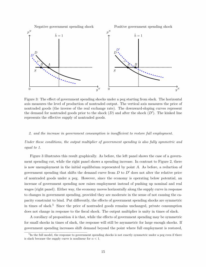
by permanently lower production and the presence of involuntary unemployment, with no tendencyto return to full employment. The economy never recovers in this version of the model, becausewages are downwardly perfectly rigid (γ = 1). Under a peg, this implies that the price of non-traded goods (or, equivalently, the real exchange rate) cannot adjust over time. In case of a float,the new equilibrium after a permanent negative shock is characterized by full employment and apermanently depreciated real exchange rate, driven by the depreciated nominal exchange rate.

Consider now the positive government spending shock, displayed in the right panel of Figure2. It shifts the demand schedule to the right, starting again from the full-employment equilibriumA. Since the economy already operates at full capacity, the additional demand is fully absorbed byan increase in the price of nontraded goods. This happens independently of whether the exchangerate is pegged or floating. In fact, given our assumptions regarding the exchange rate policy above,the increase in the price of nontraded goods is purely due to an increase in nominal wages, bothunder peg and float. For both exchange rate regimes, private consumption of nontraded goods iscompletely crowded out. The new equilibrium features unchanged levels of production of nontradedgoods and employment, while the relative price of nontraded goods is higher (real appreciation).Put differently, the fiscal multiplier on nontraded output and employment is zero.

Comparing the adjustment across the both panels of Figure 2 we stress that adjustment underthe float is symmetric, but asymmetric under the peg. We also compute impulse response functionsfor the simple model in order to illustrate the adjustment dynamics. Figure B.1 in the appendixshows the results.

13

Last, we briefly refer to Figure 2 in order to highlight a specific feature of the model in theadjustment to positive government spending shocks that are non-permanent. Consider once morethe right panel of the figure. In response to such a shock the economy first settles at point “peg”, justlike in the case of a permanent shock. Importantly, in this point nominal wages are higher than inthe initial equilibrium A. Now assume that after a while the demand curve shifts back to S becausethe level of government spending is reduced to its initial level. In this case, because nominal wagescannot fall, the supply curve cannot shift back under the peg and, hence, the economy settles at anew equilibrium with permanent unemployment. Of course, if wages are permitted to decline overtime, that is, if γ < 1, the economy will gradually converge back to point A. Still, the economy willundergo a recession once the initial fiscal stimulus is turned off. We discuss the case of temporaryshocks in more detail in Appendix B.7.

3.3 Symmetric effects under a peg in times of slack

The previous results on the asymmetric effects of government spending shocks under a peg hingeon an important assumption: that the economy is at full employment when the shock takes place.In what follows, we relax this assumption and obtain a new result for the case of an exchange ratepeg, namely that the effects of spending shocks are symmetric, provided there is sufficient slackin the economy. For this purpose, in order to induce some slack, we first introduce an additionalsurprise contractionary shock. Specifically, we assume that there is now a permanent drop in theendowment of traded goods, yTt , in period 0. The path of yTt is perfectly known at time 0 andassumed to follow the process

yTt =

1 if t < 0

yT0 < 1 if t ≥ 0 .(32)

This allows us to establish the following intermediate result.

Lemma. A drop in the endowment reduces consumption demand for traded and nontraded goods.If the exchange rate is pegged, the downward nominal wage constraint binds and both the productionof nontraded goods and employment decline. The economy operates below potential.

Intuitively, in response to the negative income shock the household lowers demand for tradedand nontraded consumption. The drop in the traded goods endowment therefore spills over intothe market for nontraded goods. To maintain full employment, the reduced demand for nontradedgoods would require the relative price of nontraded goods to fall. As this is not possible underthe peg if γ = 1, the endowment shock induces a drop in nontraded output and employment.Eventually, we are interested in how a government spending shock plays out in such situation (asopposed to full employment). The next proposition establishes our result formally.

Proposition 4. Consider an exchange-rate peg. The response of the real exchange rate to positiveand negative government spending shocks of the same size is zero and therefore symmetric, provided

1. there is slack in the economy to begin with

14

Negative government spending shock Positive government spending shockpN

0 yN

S

h = 1

DD′

AB

pN

0 yN

S

h = 1

D

A

D′

B

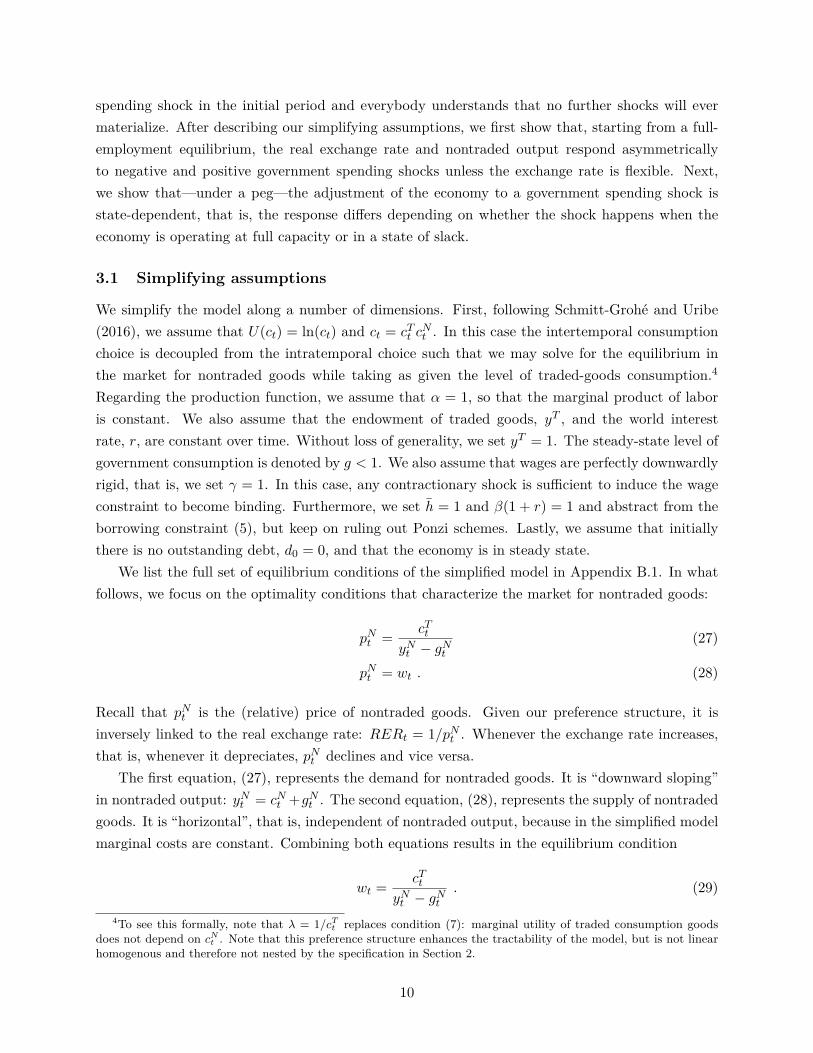
Figure 3: The effect of government spending shocks under a peg starting from slack. The horizontalaxis measures the level of production of nontraded output. The vertical axis measures the price ofnontraded goods (the inverse of the real exchange rate). The downward-sloping curves representthe demand for nontraded goods prior to the shock (D) and after the shock (D′). The kinked linerepresents the effective supply of nontraded goods.

2. and the increase in government consumption is insufficient to restore full employment.

Under these conditions, the output multiplier of government spending is also fully symmetric andequal to 1.

Figure 3 illustrates this result graphically. As before, the left panel shows the case of a govern-ment spending cut, while the right panel shows a spending increase. In contrast to Figure 2, thereis now unemployment in the initial equilibrium represented by point A. As before, a reduction ofgovernment spending that shifts the demand curve from D to D′ does not alter the relative priceof nontraded goods under a peg. However, since the economy is operating below potential, anincrease of government spending now raises employment instead of pushing up nominal and realwages (right panel). Either way, the economy moves horizontally along the supply curve in responseto changes in government spending, provided they are moderate in the sense of not causing the ca-pacity constraint to bind. Put differently, the effects of government spending shocks are symmetricin times of slack.5 Since the price of nontraded goods remains unchanged, private consumptiondoes not change in response to the fiscal shock. The output multiplier is unity in times of slack.

A corollary of proposition 4 is that, while the effects of government spending may be symmetricfor small shocks in times of slack, the response will still be asymmetric for large enough shocks. Ifgovernment spending increases shift demand beyond the point where full employment is restored,

5In the full model, the response to government spending shocks is not exactly symmetric under a peg even if thereis slack because the supply curve is nonlinear for α < 1.

15

the additional adjustment will work via prices rather than quantities, that is, the exchange ratewill appreciate. In contrast, the adjustment to spending cuts will always be through output andemployment and not via prices. We also compute the impulse responses to government spendingshocks in times of slack and show the results in Figure B.2 in the appendix.

4 Quantitative analysis

We now solve the full model, as outlined in Section 2 above. Once we relax the simplifying as-sumptions made in Section 3, the model features richer adjustment dynamics. The downside isthat we are no longer able to solve the model in closed form. Instead, we resort to numerical simu-lations which allow us to assess to what extent the asymmetry established in the previous sectionis quantitatively relevant.

We calibrate the model to capture key features of the Greek economy. This is for two reasons.First, Greece is a small open economy that operates within the euro area. From the perspectiveof the model this corresponds to an exchange-rate peg as far as the transmission of governmentspending shocks is concerned. Second, while Schmitt-Grohé and Uribe (2016) calibrate their modelto Argentina, they also consider an alternative calibration to Greece. We largely follow theircalibration—except in those instances where we explicitly account for government spending (sincethey do not).

4.1 Model calibration and solution

Table 1 summarizes the parameters of the model together with the values that we assign to themin our numerical analysis. A period in the model corresponds to one quarter. In the model, weabstract from both foreign inflation and long-run technology growth. Both factors mitigate theeffect of downward nominal wage rigidity. Following Schmitt-Grohé and Uribe (2016), we adjustthe value of γ for Greece provided in their paper by the average quarterly inflation rate in Germany(0.3% per quarter) and the average growth rate of per capita GDP in the euro periphery (0.3%).We set γ to 0.9982/(1.003 × 1.003) = 0.9922. This implies that nominal wages can fall at mostby 3.1 percent per year. We set the intra- and intertemporal elasticities of substitution betweentraded and nontraded goods, ξ and σ, to 0.44 and 5, respectively, following again Schmitt-Grohéand Uribe (2016) and Reinhart and Végh (1995). In line with the estimate of Uribe (1997), wefix the labor share in the traded goods sector at α = 0.75. We set d = 16.5418, i.e. for numericalreasons we set the upper limit 1% below the natural debt limit. We normalize the endowment ofhours h to unity. The subjective discount factor β is set to 0.9375, in line with Schmitt-Grohé andUribe (2016), to obtain a plausible foreign debt-to-GDP ratio.

We specify a VAR(1) process for the exogenous states [yTt , rt]′ on the basis of the estimatesby Schmitt-Grohé and Uribe (2016) for Greece. The steady-state endowment of traded goods isnormalized to 1, while the mean quarterly interest rate is r = 0.011. We estimate a separate AR(1)process for the exogenous state gNt , using Greek time-series data for the period 1995:Q1-2018:Q4.

16

Table 1: Parameter values used in model simulation

Parameter Value Source/Target

Wage rigidity γ = 0.9922 SGU (2016)Elasticity of substitution ξ = 0.44 SGU (2016)Risk aversion, private consumption σ=5 Standard valueLabor exponent production function α = 0.75 Uribe (1997)Debt limit d = 16.5418 99 % of natural debt limitEndowment of hours worked h = 1 NormalizationSteady state interest rate r = 0.011 Average interest rateSteady state traded goods endowment yT = 1 NormalizationSteady state government consumption gN = 0.2548 Greek government spending shareDiscount factor β = 0.9375 SGU (2016)Weight on traded goods in CES ω = 0.37 traded goods share of 0.26

To remove the growth trend, we regress the logged value on a quadratic trend. The driving processis assumed to be orthogonal to that governing [yTt , rt]′. Our empirical measure of governmentspending gNt is real public consumption provided by Eurostat (“Final consumption expenditure ofgeneral government”, P3_S13).

The resulting VAR process is given by

ln yTt

ln 1+rt1+r

ln gNtgN

=

0.88 −0.42 0−0.05 0.59 0

0 0 0.924

ln yTt−1ln 1+rt−1

1+r

ln gNt−1gN

+ εt,

εtiid∼ N

0,

5.36e− 4 −1.0e− 5 0−1.0e− 5 6.0e− 5 0

0 0 0.02282

.Finally, we pin down two further parameters as we match two key moments of the data. The

average value of government spending, gN = 0.2548, is set to match the empirical share of govern-ment consumption in GDP, pNgN/(yT +pNyN ) = 0.2123. The weight of traded goods in aggregateconsumption is determined by ω. We set it to 0.37. This implies an average share of traded goodsin total output of 26 percent, in line with the calibration target by Schmitt-Grohé and Uribe (2016).

In order to solve the model, we largely follow Schmitt-Grohé and Uribe (2016). In case of afloat, φε = 1, the lagged real wage is not a state variable and the resulting program coincides withthe central planner’s solution. This simplifies the analysis considerably and we solve the modelnumerically by value function iteration over a discretized state space. In case of a less than fullyflexible exchange rate regime, that is, if φε < 1, the lagged real wage is a state variable, as isthe external debt position. To solve the model in this case, we resort to Euler equation iteration.

17

Appendix C.1 provides details on the discretization of the state space while Appendix C.2 reportsthe unconditional moments of the model.

4.2 Model impulse responses

Figure 4 displays the model impulse responses to a government spending shock. Here we showgeneralized impulse response functions (GIRFs) in order to account for nonlinear adjustment dy-namics in the model: for a given initial point in the state space, we compare how variables evolveover time in response to a shock relative to what happens in a baseline scenario where the shockdoes not occur. We then average over one million replications to integrate out the effect of futureshocks. We consider both positive and negative shocks equal to ±2.2 percentage points of steadystate nontraded output. This corresponds to a one-standard-deviation shock. In the figure, thesolid lines represent the dynamics due to a spending increase, while the dashed lines correspond toa spending cut. We report the responses for the first 8 quarters after a shock.

In the left column, we show results assuming flexible exchange rates. Recall that in this casethe exchange rate is used to stabilize output at the full-employment level. In the middle column,we show results for an economy that features an exchange-rate peg and initially operates at fullcapacity. In the right-most column, instead, we consider an exchange rate peg with economic slack,captured by simulations with an average unemployment rate of 14%.6 We also compute impulseresponses for an intermediate exchange rate regime and find, perhaps unsurprisingly, that they arein between those obtained for the peg and the pure float (see Figure C.5 in the appendix).

The panels in the top row of Figure 4 show the dynamics of government spending. Sincegovernment spending is determined exogenously, the dynamics are the same across all columns.The second and third row show the adjustment of nontraded output, yN , and the real exchangerate, RER, respectively.7 Notice that, as before, a decline of RER represents a real appreciation.

Overall, we find that the qualitative results established in Section 3 above turn out to bequantitatively important. A number of points are particularly noteworthy. First, as establishedin Proposition 1, a cut of government spending (dashed lines) depreciates the real exchange rateunder a float (left column), and nontraded output is fully stabilized. In contrast, under a peg(middle and right column), the real exchange rate response is much weaker. Now, and in contrastto Section 3, because we no longer restrict wages to be completely downwardly rigid, the exchangerate does adjust over time. However, its response is still very much muted compared to the float.As a consequence, nontraded output declines strongly and persistently in response to the spending

6Using different initial conditions for the scenarios allows us to capture the role of economic slack. In addition,we also allow for small variations in the initial debt level in order to minimize nonlinear interaction effects of theinitial debt level and the government spending shock. We assume values in the range of 98-99% of the ergodic mean.Under the peg with full employment we set d0 = 13.2276 and w−1 = 1.7637, for the float we set d0 = 14.1672. Theexogenous states are set to their steady-state values. For the peg with slack we draw from the ergodic distributionby first simulating the model for a burn-in period of 300 quarters.

7The exchange rate is measured in percent of the ergodic mean. Government spending and nontraded outputare measured in percent of nontraded output under full employment. The latter normalization is used for bettercomparability. If we were to use the ergodic mean for nontraded output, the scaling of the IRFs would be affectedby the different unemployment rates in the ergodic distribution across exchange rate regimes.

18

Float Peg (full employment) Peg (slack)gN

(%ofyN)

yN

(%ofyN)

gov. spending increasegov. spending cut

RER

(%of

erg.

mean)

quarter quarter quarter

Figure 4: Generalized impulse responses to one-standard-deviation government spending shocks.Solid line: spending increase, dashed line: spending cut. Left column: flexible exchange rate.Middle: exchange rate peg and full employment, right: peg and economic slack. Top panels:government spending, middle: nontraded output, bottom: real exchange rate. Horizontal axismeasures time in quarters, vertical axis measures effect of shock in percent of full employmentnontraded output yN and of the ergodic mean of the RER, respectively.

cut.Second, turning to positive spending shocks (solid lines), we obtain dynamics in line with

Proposition 2. On impact, the adjustment is independent of the exchange rate regime providedthere is full employment. Output does not fall, and the exchange rate depreciates for reasonsdiscussed in Section 3 above. However, as we simulate the full model, we now observe richeradjustment dynamics. While initially unaffected, output declines somewhat over time under thepeg because the shock process is mean-reverting rather than permanent. As government spendinggradually returns to its pre-shock level, real wages and the real exchange rate are required todecline in order to maintain full employment. This is what happens under the float (left column).Yet it happens more slowly under the peg (middle panel) because of the downward nominal wage

19

rigidity.8 Hence, we find that under a peg (with full employment) the impact multiplier of positivegovernment spending shocks on output is zero. It is negative in the short run.

Third, we find that the real exchange rate response is symmetric under a float, as establishedin Proposition 3. It is asymmetric under a peg with full employment. Positive shocks appreciatethe real exchange rate, whereas negative spending shocks do induce some depreciation in the fullmodel, because wages are not fully downwardly rigid and the supply curve is upward sloping. Yet,the exchange rate response to spending cuts is one order of magnitude weaker than that to spendingincreases. Just like for the response of the real exchange rate, the asymmetry is quite strong fornontraded output, too.

Fourth, we find that the adjustment under a peg is symmetric if there is slack, consistent withProposition 4 above. This holds both for the exchange rate and for output. In contrast to what weestablished for the simplified model, we now observe that the real exchange rate actually moves,because the supply curve is not perfectly horizontal (α < 1) and nominal wages are allowed to fallsomewhat (γ < 1). But the exchange rate response is considerably weaker compared to the case offull employment.

5 Empirical evidence

In this section, we provide new evidence on how government spending impacts the real exchangerate. A number of earlier studies have explored the issue and reported different, partly conflictingresults regarding the sign of the response (e.g. Corsetti et al., 2012a; Ilzetzki et al., 2013; Kim andRoubini, 2008; Monacelli and Perotti, 2010; Ravn et al., 2012). In what follows we take a freshlook: informed by the model-based analysis above, we ask whether spending increases and cutsimpact the real exchange rate symmetrically or not.

Our analysis builds on Born et al. (2019), both in terms of data and in terms of identification.Our sample covers observations for 38 emerging and advanced economies. We consider two identi-fication schemes going back to Blanchard and Perotti (2002) and Ramey (2011b), respectively (seealso Ramey and Zubairy (2018) for a recent discussion). In both instances, the idea is to measurethe surprise component of government spending, in the first case on the basis of an estimated vectorautoregressive (VAR) model, in the second case on the basis of professional forecasts. In terms ofidentification, we assume that both fiscal surprise measures do not reflect an endogenous responseof fiscal policy to other innovations in the economy. As a result, we may interpret them as shocks.We establish their effect on government spending, output, and the real exchange rate by means oflocal projections à la Jordà (2005).

5.1 Empirical specification

We briefly outline our empirical specification. It establishes the effect of government spending onthe exchange rate on the basis of fiscal shocks, εgi,t, computed in a first step. Here, indices i and t

8See also Figure B.3 in the appendix.

20

refer to country i and period t, respectively. We provide more details below.In a second step, we estimate local projections, which are particularly suited to account for

potentially asymmetric effects of positive and negative shocks. Specifically, we sort fiscal shocksaccording to their sign and define εg+i,t = εgi,t if ε

gi,t ≥ 0 and 0 otherwise, and analogously for negative

shocks, εg−i,t (see Kilian and Vigfusson, 2011, for this approach). Letting xi,t+h denote the variableof interest in period t+ h, we estimate how it responds to fiscal shocks in period t on the basis ofthe following specification:

xi,t+h = αi,h + ηt,h + ψ+h ε

g+i,t + ψ−h ε

g−i,t + γZi,t + ui,t+h . (33)

Here, the coefficients ψ+h and ψ−h provide a direct estimate of the impulse response at horizon h

to a positive and negative shock, respectively. Zi,t is a vector of control variables. The error termui,t+h is assumed to have zero mean and strictly positive variance. αi,h and ηt,h denote country andtime fixed effects. We compute standard errors that are robust with respect to heteroskedasticityas well as serial and cross-sectional correlation (Driscoll and Kraay, 1998).

5.2 Identification

Our identification strategy is explained in Born et al. (2019) in some detail. Here we summarize theessential aspects. Importantly, we pursue two alternative strategies to construct fiscal innovations.One strategy has been introduced by Ramey (2011b). The idea is simply to purge actual governmentspending growth of what professional forecasters project spending growth to be. Formally, we have

εgi,t = ∆gi,t − Et−1∆gi,t ,

where ∆gi,t is the realization of government consumption growth and Et−1∆gi,t is the previousperiod’s forecast.

The second strategy employs a panel VAR model to compute spending surprises. LetXi,t denotea vector of endogenous variables, which includes government spending and output. We estimatethe following model:

Xi,t = αi + ηt +A(L)Xi,t−1 + νi,t,

where A(L) is a lag polynomial and νi,t is a vector of reduced-form disturbances with covariancematrix E(νi,tν ′i,t) = Ω. In our analysis below we allow for four lags since the model is estimatedon quarterly data. Assuming i) a lower Cholesky factorization L of Ω, and ii) that governmentconsumption growth is ordered on top in the vector Xi,t, the structural shock εgi,t equals the (scaled)first element of the reduced-form disturbance vector νi,t, i.e. εgi,t = L−1νi,t.9

Our identifying assumption, dating back to Blanchard and Perotti (2002), is that the forecasterror of government spending growth is not caused by contemporaneous innovations, so that it

9The estimated shocks εgi,t in this specification are generated regressors in the second stage. However, as shownin Pagan (1984), the standard errors on the generated regressors are asymptotically valid under the null hypothesisthat the coefficient is zero; see also Coibion and Gorodnichenko (2015), footnote 18, on this point.

21

represents a genuine fiscal shock. We make the same assumption with regard to both measures offiscal surprises, those obtained in the VAR setting and those obtained on the basis of professionalforecasts. It is also implicit in Ramey (2011b), as she considers a measure of fiscal shocks based onprofessional forecasts. For identification to go through, her (implicit) assumption is that surpriseinnovations do not represent an endogenous response to other shocks. As discussed by Blanchardand Perotti (2002), the rationale for this assumption is that government spending can be adjustedonly subject to decision lags. Also, there is no automatic response, since government consumptiondoes not include transfers or other cyclical items.

5.3 Data

Our data set covers 38 countries and contains quarterly observations starting in the early 1990s andending in 2018. See Table D.2 in the appendix for specific information on the country coverage andBorn et al. (2019) for more details on the data set. Our measure of the real exchange rate is thebroad real effective exchange rate index compiled by the BIS, complemented by data for Ecuador,El Salvador, and Uruguay based on the data for 38 trading partners compiled by Darvas (2012).Our quarterly measure is the logarithm of the average of the monthly index values. An increase inthe index indicates a depreciation of the economy’s currency against a broad basket of currencies.We proxy nontraded output by real GDP. Our measures of real GDP and government consumptionare based on national accounts data. The vector of controls in the local projection (33) featuresfour lags of log real government consumption, log real output, log real effective exchange rate, andthe sovereign default premium to control for fiscal stress. The sovereign default premium measuresthe spread between foreign currency debt and the risk-free rate and is the end-of-quarter value. Weallow for country-specific linear time trends in output and government spending. When conditioningon inflation and labor market slack, we use year-on-year GDP deflator inflation and unemploymentas a percentage of the active population from the EU-LFS main indicators, respectively.

Professional forecasts are due to Oxford Economics and available for a subset of countries only.Instead, we are able to compute the VAR-based forecast error for all 38 countries. Table 2 providesa number of basic summary statistics regarding the forecast errors. Over the full sample, theaverage forecast errors are close to zero, by construction in the case of the VAR-based measure. Onan individual country basis, Oxford Economics produces forecasts with a relatively low root meansquared error (RMSE). The VAR forecasts exhibit a somewhat larger RMSE, but note that in thiscase the sample is more challenging.

In the last row of Table 2, we report a measure of the predictive power of the shocks for actualgovernment spending growth in the form of an F-statistic along the lines of the tests conducted inRamey (2011b) and Ramey and Zubairy (2018).10 We find that the shock measure based on the

10Technically, given our panel structure with potentially non i.i.d. errors, we follow the suggestion in Baum etal. (2007) and check the predictive power of our identified shocks using the Kleibergen and Paap (2006) rk WaldF -statistic. It is computed in a “first-stage” panel fixed effects regression of the government consumption growthvariable on the respective shock measure. Computing “naive” F -statistics in our pooled sample yields very similarvalues.

22

Table 2: Forecast errors of government consumption growth: descriptive statistics

Prof. Forecasts VAR

Countries 23 38Observations 1696 2944Mean -0.016 0.000RMSE 0.616 1.954Wald F -statistic 4.9 849.2

Notes: Forecast errors measured in percentage points. Kleibergen and Paap (2006) rk-Wald F -statistic computed using Stata’s xtivreg2 in a first-stage regression of government consumptiongrowth on the respective forecast error. Robust covariance estimator clustered at country andquarter level. Professional forecasts are based on Oxford Economics.

forecasts of Oxford Economics do not pass the rule-of-thumb threshold of 10 proposed by Staigerand Stock (1997), while the VAR-based measure does with flying colors.11

5.4 Results

We now report our results for both shock measures. Consider Figure 5 first. It shows the resultsbased on the VAR forecast error. The left column displays the impulse responses to a negativegovernment spending shock, the right column displays the responses to a positive shock. Through-out, solid lines represent the point estimate, while the dark (and light) shaded areas indicate 68(and 90) percent confidence intervals. We measure the time after impact along the horizontal axisin quarters and the effect of the shock along the vertical axis in percentage deviation from thepre-shock level. The response of government spending, shown in the top row, is fairly persistent inboth cases, albeit more so in case of a hike (right column). We show the response of output in themiddle row and observe that it is fairly symmetric. Not only is the initial response comparable inabsolute value, the ensuing adjustment pattern is also quite similar. The strongest output effectobtains between 1 and 1.5 years after impact. Afterwards, output starts to converge back to itspre-shock level. From a quantitative point of view, the output response suggests a multiplier effectwhich is in line with earlier studies as surveyed, for instance, by Ramey (2011a). Assuming thatgovernment consumption accounts for about 15 percent of GDP on average, our finding that achange in government spending by one percent changes output by about 0.1 percent on impact,and by about 0.2 after approximately 1 to 2 years, implies a multiplier effect of about 0.67 and1.33, respectively.12

11The Montiel Olea and Pflueger (2013)-threshold for the 5 percent critical value for testing the null hypothesisthat the 2SLS bias exceeds 10 percent of the OLS bias in our context is 23.1. The results for the measure basedon professional forecasts are more favorable once we assess its predictive power for government spending as reportedby Oxford Economics in real time, which is the relevant measure for the financial markets’ assessment of currentconditions, see Born et al. (2019). In the present paper, we focus on actual government spending as reported in theNIPA, in line with the model analysis performed above.

12Note that this ex-post conversion is meant as a rule-of-thumb conversion. See Ramey and Zubairy (2018) on theintricacies of computing output multipliers.

23

Negative shock Positive shock

Gov

spen

ding

Outpu

tEx

chan

gerate

quarter quarter

Figure 5: Adjustment to government spending shock. Identification based on VAR forecast error.Solid lines represent point estimates, light (dark) shaded areas represent 90 (68) percent confidenceintervals. Horizontal axis measures time in quarters. Vertical axis measures deviation from pre-shock level in percent.

Last, we turn to the response of the real exchange rate, shown in the bottom row of Figure 5.We find that a cut of government spending depreciates the real exchange rate—i.e. the price offoreign consumption in terms of domestic consumption goes up. In contrast, a spending increaseappreciates it—i.e. the price of foreign consumption declines. The adjustment pattern is not fullysymmetric. In particular, the exchange rate responds more strongly in the short run if spending is

24

Negative shock Positive shock

Gov

spen

ding

Outpu

tEx

chan

gerate

quarter quarter

Figure 6: Adjustment to government spending shock. Identification based on forecast error ofprofessional forecasters. Solid lines represent point estimates, light (dark) shaded areas represent90 (68) percent confidence intervals. Horizontal axis measures time in quarters. Vertical axismeasures deviation from pre-shock level in percent.

cut and more strongly in the medium run if government spending is raised. By and large, however,we fail to detect a strong asymmetry in the exchange rate response, and even less so for output.This result conforms well with the predictions of the model to the extent that there are manycountries in our sample operating a flexible exchange rate regime—see Section 3 above.

Our result is also robust across shock measures. This becomes clear as we turn to Figure 6,

25

which shows results for fiscal shocks computed on the basis of forecast errors of professional (ratherthan VAR) forecasts. Note that in this case our sample is quite a bit smaller because we lackprofessional forecasts for a number of countries—see again Table D.2. And yet, even though thesample differs considerably, we find that the results shown in Figure 6 are comparable to thoseshown in Figure 5 above.

We again report the response of actual government spending in the top row, both to negativespending shocks (left column) and to positive spending shocks (right column). A noteworthydifference vis-à-vis the results shown in Figure 5 is that the response of government spendingis quite a bit weaker—in general and on impact in particular. This reflects the fact that here wecompute forecast errors on the basis of real-time forecasts and hence their effect on actually realizedgovernment spending is limited. This is also reflected in the F-statistic reported in the last row ofTable 2 above.

And yet, the responses of output and the real exchange rate shown in Figure 6 are fairly similarto those shown in Figure 5 above. In particular, in Figure 6 we again observe a fairly symmetricoutput response and a pattern of the exchange rate adjustment that resembles the one shown inFigure 5 rather closely. We note, however, that the depreciation of the exchange rate in response tothe spending cut is no longer significant—as our model-based analysis predicts for countries witha fixed exchange rate regime.

The central prediction of the model put forward in Section 3 above is that whether or notgovernment spending shocks impact the real exchange rate asymmetrically depends on the exchangerate regime. There should be no asymmetric effects in case the exchange rate floats freely, butsignificant asymmetries under an exchange-rate peg. To explore this aspect further, we focus onthe countries in the euro area.13 Here the nominal exchange rate is permanently fixed and may notbring about the necessary adjustment of the real exchange rate in response to government spendingshocks. Note that we rely only on the VAR-based forecast errors as we turn to the countries in theeuro area because for this subsample we find that the forecast errors based on professional forecastshardly impact actual government spending at all (the Wald F -statistic is 0.528 in this case). As aresult, we are unable to obtain reliable estimates for this subsample once we use the shock measurecomputed on the basis of professional forecasts. The VAR-based shocks remain strong predictorsof actual government spending (the Wald F -statistic is 376.14 in this case).

We report the results for the panel composed of the individual countries of the euro area inFigure 7. The figure is organized just like Figures 5 and 6 above. The fiscal shocks are computedon the basis of an estimated VAR model, as in Figure 5. The only difference is the underlyingsample, since Figure 7 shows the results for euro area countries only. This has a strong bearing onthe results.

The response of government spending (shown again in the top row) is fairly symmetric forspending cuts and spending hikes as before. However, we now find the model predictions fully

13Here we restrict our sample to observations for euro area countries after their exchange rates vis-à-vis the eurohave been “irrevocably” fixed—see Table D.2 for the detailed sample coverage.

26

Negative shock Positive shock

Gov

spen

ding

Outpu

tEx

chan

gerate

quarter quarter

Figure 7: Adjustment to government spending shock in individual countries of the euro area.Identification based on VAR forecast error. Solid lines represent point estimates, light (dark)shaded areas represent 90 (68) percent confidence intervals. Horizontal axis measures time inquarters. Vertical axis measures deviation from pre-shock level in percent.

borne out by the evidence: output drops in response to a spending cut, but is virtually unchangedif government spending is raised. Instead, the exchange rate does not respond to a spending cut, butappreciates in response to a spending increase. We stress once more that the asymmetry obtainsonly once we restrict our sample to countries that operate under fixed exchange rate—just like themodel in Section 3 above predicts.

27

Negative shock Positive shock

Gov

spen

ding

Outpu

tEx

chan

gerate

quarter quarter

Figure 8: Adjustment to government spending shock in individual countries of the euro area wheninflation is above 3 percent (dashed lines) and in the baseline euro-area sample (solid lines). Solidand dashed lines represent point estimates, shaded areas represent 90 percent confidence intervals.Horizontal axis measures time in quarters. Vertical axis measures deviation from pre-shock level inpercent.

In the model, the asymmetric response to government spending shocks under a peg is caused bydownward nominal wage rigidity. It prevents real wages to decline in response to a spending cut,but does not prevent them from rising in response to spending increase. Yet, if inflation is highto begin with, downward nominal wage rigidity should have less of a bearing on the adjustment

28

because in this case wages are adjusting in real terms, even if they are nominally rigid. To assessthis implication of the model empirically, we estimate our empirical specification once more on theindividual countries of the euro area but focus on high-inflation periods. Specifically, we specifya threshold for year-on-year inflation of 3 percent. In our sample, 25 percent of the observationsqualify as high-inflation episodes on the basis of this definition.14 We repeat our second-stageestimation on the high-inflation observations.

Figure 8 shows the results. The organization of the figure mimics again those of the figuresabove. However, we now show distinct impulse responses for high-inflation episodes (dashed lines)and contrast them with the baseline case for the euro area (solid lines). Here shaded areas indicate90 percent confidence intervals. Overall we find that the adjustment dynamics are quite similar.However, there are also some differences and they align well with theory. In particular, we find that,in response to a spending cut, the exchange rate tends to depreciate when inflation is high. Putdifferently, the response of the exchange rate to government spending shocks is again symmetricprovided that inflation is high—even if countries operate under a fixed exchange rate regime.Moreover, as the exchange rate depreciates in response to a spending cut, output tends to declineless during high-inflation periods compared to the baseline. Whether inflation is high or not, instead,turns out to be largely inconsequential for the adjustment to spending hikes. Once more, thesefindings lend support to the model predictions derived in Section 3 above. For the model predictsthat, in response to a positive spending shock, downward nominal wage rigidity is inconsequential.It is only in response to a spending cut that it matters—provided that inflation is sufficiently low.

In a last experiment, we condition the effects of government spending shocks on the extent ofeconomic slack. In earlier empirical work Auerbach and Gorodnichenko (2012, 2013) find that theeffects of fiscal policy are stronger in a recession than they are in a boom. Ramey and Zubairy(2018) instead find that multipliers generally do not depend on the extent of slack in the economy.Our model with DNWR provides a refinement for fixed exchange rate regimes. It predicts thateconomic slack alters the effects of government spending shocks, but only those of positive shocks.Raising government spending in times of slack should impact output rather than the exchange rate,as opposed to when the economy is operating at full capacity. Put differently, the model predictsthat, in times of slack, government spending shocks impact the economy symmetrically, even ifthere is an exchange rate peg.

We now take up this issue empirically and estimate the model for episodes of economic slack,again only within the euro-area sample. For this purpose we include only observations in our samplefor which unemployment is above a country’s median unemployment value, as in Barro and Redlick(2011). Figure 9 shows the results. Consider first the left column: as predicted by the model, slack(red line) does not alter the response to a spending cut relative to the baseline (blue line). Outputcontracts and the real exchange rate does not adjust. However, slack does alter the response toa spending hike. Just like the model predicts, output rises in response to a spending increase intimes of slack, while the exchange rate response is muted and basically insignificant.

14This threshold is high enough for Germany to never experience a high-inflation episode.

29

Negative shock Positive shock

Gov

spen

ding

Outpu

tEx

chan

gerate

quarter quarter

Figure 9: Adjustment to government spending shock in individual countries of the euro area intimes of slack (dashed lines) and in the baseline euro-area sample (solid lines). Solid and dashedlines represent point estimates, shaded areas represent 90 percent confidence intervals. Horizontalaxis measures time in quarters. Vertical axis measures deviation from pre-shock level in percent.

In sum, we find that the empirical evidence on the effects of government spending shocks alignswell with the predictions of the model. This holds for our main result, namely that economies withfixed exchange rates respond asymmetrically to positive and negative shocks. But it also holds forthe predictions regarding the specific role of DNWR and economic slack.

30

6 Conclusion

We show that the adjustment to government spending shocks is asymmetric under fixed exchangerates. Assuming full employment, an increase of government spending appreciates the real exchangerate and does not impact output and employment. A reduction of government spending, instead,lowers output and employment and does not impact the exchange rate very much. We derive theseresults in a stylized model of a small open economy which features downwardly rigid nominal wagesas in Schmitt-Grohé and Uribe (2016). We establish new evidence based on a large panel data setand show that the predictions of the model are borne out in the data along several dimensions: theexchange rate regime, the state of the business cycle, and the level of inflation.

Our result has the potential to reconcile Keynesian and classical views on the role of fiscal sta-bilization policy in open economies. The Keynesian view holds that fiscal policy impacts economicactivity strongly if the nominal exchange rate is fixed. According to the classical view, fiscal policyimpacts mostly prices. In light of our analysis, both views appear to be (somewhat) correct—itis just a matter of the sign of the fiscal impulse. In a sense, this is bad news because raisinggovernment spending is likely to only appreciate the exchange rate, while austerity is likely to beparticularly detrimental to economic activity.

Yet, our analysis also provides a rigorous argument for a strongly countercyclical conduct offiscal policy under fixed exchange rates. After all, our results suggest that cutting governmentspending during booms is highly effective in reducing inflationary pressures, while raising spendingin deep recessions boosts output and employment considerably. However, in conclusion, we alsonote that our analysis is purely positive and any policy conclusion is therefore tentative. We leavea rigorous analysis of optimal fiscal policy in this framework for future work.

31

References

Auerbach, Alan J. and Yuriy Gorodnichenko (2012). “Measuring the output responses to fiscalpolicy”. American Economic Journal: Economic Policy 4 (2), 1–27.

(2013). “Fiscal multipliers in recession and expansion”. Fiscal policy after the financialcrisis. Ed. by Alberto Alesina and Francesco Giavazzi. Chicago: University of Chicago Press,63–98.

Barro, Robert J. and Charles J. Redlick (2011). “Macroeconomic effects from government purchasesand taxes”. Quarterly Journal of Economics 126 (1), 51–102.

Baum, Christopher F., Mark E. Schaffer, and Steven Stillman (2007). “Enhanced routines forinstrumental variables/generalized method of moments estimation and testing”. Stata Journal7 (4), 465–506.

Bénétrix, Agustín S. and Philip R. Lane (2013). “Fiscal shocks and the real exchange rate”. Inter-national Journal of Central Banking 9 (3), 6–37.

Benigno, Pierpaolo and Luca Antonio Ricci (2011). “The inflation-output trade-off with downwardwage rigidities”. American Economic Review 101 (4), 1436–1466.

Betts, Caroline and Michael B. Devereux (2000). “Exchange rate dynamics in a model of pricing-to-market”. Journal of International Economics 50 (1), 215–244.

Bianchi, Javier, Pablo Ottonello, and Ignacio Presno (2019). “Fiscal stimulus under sovereign risk”.Mimeo.

Blanchard, Olivier J. and Roberto Perotti (2002). “An empirical characterization of the dynamiceffects of changes in government spending and taxes on output”. Quarterly Journal of Economics117 (4), 1329–1368.

Born, Benjamin, Falko Juessen, and Gernot J. Müller (2013). “Exchange rate regimes and fiscalmultipliers”. Journal of Economic Dynamics and Control 37 (2), 446–465.

Born, Benjamin, Gernot J. Müller, and Johannes Pfeifer (2019). “Does austerity pay off?” Reviewof Economics and Statistics.

Burgert, Matthias, Philipp Pfeiffer, and Werner Roeger (2019). “Fiscal policy in EMU with down-ward nominal wage rigidity”. Mimeo.

Christiano, Lawrence J., Martin Eichenbaum, and Sergio Rebelo (2011). “When is the governmentspending multiplier large?” Journal of Political Economy 119 (1), 78–121.

Coibion, Olivier and Yuriy Gorodnichenko (2015). “Information rigidity and the expectations for-mation process: a simple framework and new facts”. American Economic Review 105 (8), 2644–2678.

Corsetti, Giancarlo, Keith Kuester, André Meier, and Gernot J. Müller (2013a). “Sovereign risk,fiscal policy, and macroeconomic stability”. Economic Journal 123 (566), F99–F132.

Corsetti, Giancarlo, Keith Kuester, and Gernot J. Müller (2013b). “Floats, pegs, and the transmis-sion of fiscal policy”. Fiscal policy and macroeconomic performance. Ed. by Jordi Galí and LuisCespedes. Vol. 17. Central Banking, Analysis, and Economic Policies. Central Bank of Chile.Chap. 7, 253–287.

32

Corsetti, Giancarlo, André Meier, and Gernot J. Müller (2012a). “Fiscal stimulus with spendingreversals”. Review of Economics and Statistics 94 (4), 878–895.

(2012b). “What determines government spending multipliers?” Economic Policy (72), 521–565.

Corsetti, Giancarlo and Gernot J. Müller (2006). “Twin deficits: squaring theory, evidence andcommon sense”. Economic Policy 48 (48), 598–638.

Darvas, Zsolt (2012). “Real effective exchange rates for 178 countries: a new database”. WorkingPaper 2012/06. Bruegel.

Driscoll, John C. and Aart C. Kraay (1998). “Consistent covariance matrix estimation with spatiallydependent panel data”. The Review of Economics and Statistics 80 (4), 549–560.

Dupraz, Stéphane, Emi Nakamura, and Jón Steinsson (2019). “A plucking model of business cycles”.Mimeo.

Elsby, Michael W. L. and Gary Solon (2019). “How prevalent is downward rigidity in nominal wages?international evidence from payroll records and pay slips”. Journal of Economic Perspectives33 (3), 185–201.

Enders, Zeno, Gernot J. Müller, and Almuth Scholl (2011). “How do fiscal and technology shocksaffect real exchange rates?” Journal of International Economics 83 (1), 53–69.

Erceg, Christopher J. and Jesper Lindé (2012). “Fiscal consolidation in an open economy”. Amer-ican Economic Review 102 (3), 186–91.

Farhi, Emmanuel and Ivan Werning (2016). “Fiscal multipliers”. Handbook of macroeconomics. Ed.by John B. Taylor and Harald Uhlig. Vol. 2. Elsevier. Chap. 31, 2417–2492.

Giavazzi, Francesco, Tullio Jappelli, and Marco Pagano (2000). “Searching for non-linear effects offiscal policy: evidence from industrial and developing countries”. European Economic Review44 (7), 1259–1289.

Ilzetzki, Ethan, Enrique G. Mendoza, and Carlos A. Végh (2013). “How big (small?) are fiscalmultipliers?” Journal of Monetary Economics 60 (2), 239–254.

Jo, Yoon J. (2018). “Downward nominal wage rigidity in the United States”. Mimeo. ColumbiaUniversity.

Jordà, Òscar (2005). “Estimation and inference of impulse responses by local projections”. AmericanEconomic Review 95 (1), 161–182.

Kilian, Lutz and Robert J. Vigfusson (2011). “Are the responses of the U.S. economy asymmetricin energy price increases and decreases?” Quantitative Economics 2 (3), 419–453.

Kim, Soyoung and Nouriel Roubini (2008). “Twin deficit or twin divergence? Fiscal policy, currentaccount, and real exchange rate in the U.S.” Journal of International Economics 74 (2), 362–383.

Kleibergen, Frank and Richard Paap (2006). “Generalized reduced rank tests using the singularvalue decomposition”. Journal of Econometrics 133 (1), 97–126.

Kollmann, Robert (2010). “Government purchases and the real exchange rate”. Open EconomiesReview 21 (1), 49–64.

33

Liu, Siming (2018). “Government spending during sudden stop crises”. Mimeo.Miyamoto, Wataru, Thuy Lan Nguyen, and Viacheslav Sheremirov (2019). “The effects of govern-

ment spending on real exchange rates: evidence from military spending panel data”. Journal ofInternational Economics 116, 144–157.

Monacelli, Tommaso and Roberto Perotti (2010). “Fiscal policy, the real exchange rate and tradedgoods”. Economic Journal 120 (544), 437–461.

Montiel Olea, José Luis and Carolin Pflueger (2013). “A robust test for weak instruments”. Journalof Business & Economic Statistics 31 (3), 358–369.

Nakamura, Emi and Jón Steinsson (2014). “Fiscal stimulus in a monetary union: evidence from USregions”. American Economic Review 104 (3), 753–92.

Pagan, Adrian (1984). “Econometric issues in the analysis of regressions with generated regressors”.International Economic Review 25 (1), 221.

Ramey, Valerie A. (2011a). “Can government purchases stimulate the economy?” Journal of Eco-nomic Literature 49 (3), 673–685.

(2011b). “Identifying government spending shocks: it’s all in the timing”. Quarterly Journalof Economics 126 (1), 1–50.

(2019). “Ten years after the financial crisis: what have we learned from the renaissance infiscal research?” Journal of Economic Perspectives 33 (2), 89–114.

Ramey, Valerie A. and Sarah Zubairy (2018). “Government spending multipliers in good times andin bad: evidence from US historical data”. Journal of Political Economy 126 (2), 850–901.

Ravn, Morten O., Stephanie Schmitt-Grohé, and Martín Uribe (2012). “Consumption, governmentspending, and the real exchange rate”. Journal of Monetary Economics 59, 215–234.

Reinhart, Carmen M. and Carlos A. Végh (1995). “Nominal interest rates, consumption booms,and lack of credibility: a quantitative examination”. Journal of Development Economics 46 (2),357–378.

Schmitt-Grohé, Stephanie and Martín Uribe (2014). “Finite-state approximation of VAR processes:a simulation approach”. Mimeo.

(2016). “Downward nominal wage rigidity, currency pegs, and involuntary unemployment”.Journal of Political Economy 124 (5), 1466–1514.

Shen, Wenyi and Shu-Chun S. Yang (2018). “Downward nominal wage rigidity and state-dependentgovernment spending multipliers”. Journal of Monetary Economics 98, 11–26.

Sinn, Hans-Werner (2014). “Austerity, growth and inflation: remarks on the eurozone’s unresolvedcompetitiveness problem”. The World Economy 37 (1), 1–31.

Staiger, Douglas and James H. Stock (1997). “Instrumental variables regression with weak instru-ments”. Econometrica 65 (3), 557–586.

Tauchen, George and Robert Hussey (1991). “Quadrature-based methods for obtaining approximatesolutions to nonlinear asset pricing models”. Econometrica 59 (2), 371.

Uribe, Martín (1997). “Exchange-rate-based inflation stabilization: the initial real effects of credibleplans”. Journal of Monetary Economics 39 (2), 197–221.

34

Appendix

A Full set of equilibrium conditions (baseline model)

Definition 1. An equilibrium is defined as a set of stochastic processes cTt , ht, dt+1, wt, λt, µt, ∞t=0satisfying

cTt = yTt − dt + dt+11 + rt

(A.1)

λt = ω

[ω(cTt )

ξ−1ξ + (1− ω)(hαt − gNt )

ξ−1ξ

] ξξ−1 ( 1

ξ−σ)

(cTt )−1σ (A.2)

λt1 + rt

= βEtλt+1 + µt (A.3)

µt ≥ 0 ∧ dt+1 ≤ d with 0 = µt(dt+1 − d) (A.4)

wt

αhα−1t

= 1− ωω

(cTt

hαt − gNt

) 1ξ

(A.5)

wt ≥ γwt−1εt

(A.6)

ht ≤ h (A.7)

0 = (h− ht)(wt − γ

wt−1εt

), (A.8)

as well as a suitable transversality condition, given initial conditions w−1, d0, exogenous stochasticprocesses yTt , rt, gNt ∞t=0, and an exchange rate policy εt∞t=0.

35

B Analytical model

B.1 Full set of equilibrium conditions (simplified model)

Given the preferences and the functional forms assumed in Section 3, we obtain the followingequilibrium conditions:

cTt = 1− dt + dt+11 + r

(B.1)

yNt = ht = cNt + gNt (B.2)1cTt

= 1cTt+1

(B.3)

pNt = cTtht − gNt

(B.4)

pNt = wt (B.5)

RERt = 1pNt

(B.6)

wt ≥wt−1εt∧ ht ≤ 1 with 0 = (1− ht)

(wt −

wt−1εt

)(B.7)

wft = cTt1− gNt

(B.8)

εt = maxwt−1

wft, 1φε

(B.9)

0 = limj→∞

( 11 + r

)jdt+j . (B.10)

Consequently, the initial steady state is given by d−1 = 0, cT−1 = yT = 1, cN−1 = 1 − g, where gdenotes the steady state value of government consumption, pN−1 = w−1 = 1

1−g , and RER−1 = 1−g.

B.2 Proof Proposition 1

The Euler equation (B.3) implies that traded consumption is constant at its new value, i.e.,cTt = cTt+1 for all t ≥ 0. The resource constraint (B.1) then implies dt+1

1+r − dt = dt+21+r − dt+1

for all t ≥ 0. Thus, if there is any increase in debt in one period, debt will keep increasing. Thisis a reflection of the well-known random walk property of consumption in this type of setup. Anyincrease in additional traded consumption financed by debt persists in future periods and, givena constant endowment yT , needs to be financed by further additional debt issuance. Because thiscontinuing debt accumulation would violate the transversality condition (B.10), debt needs to beconstant at its initial value of 0, i.e., dt = 0 and cTt = yT = 1 for all t ≥ 0.15 In period 0, thenontraded goods resource constraint (B.2) implies cN0 = yN0 − g, while equations (B.4) and (B.5)

15A different way to see this is to notice that this equation is a homogenous second-order difference equation withroots (1 + r) and 1. Given d0 and the transversality condition, the unstable root can be ruled out.

36

imply that the real wage is given by w0 = 1h0−g . Thus, we need to solve for nontraded output yN0

and hours worked h0, which both depend on the exchange rate arrangement.

Peg (φε = 0): Conjecture that the economy is in a situation of unemployment with h0 < 1.In this case, the wage constraint (B.7) must be binding: w0 = w−1

ε0. Under the peg, the gross

nominal exchange rate devaluation is given by ε0 = 1. Consequently, the real wage is given byw0 = 1

h0−g = 11−g = w−1, which implies 1− g = h0− g < 1− g. This, in turn, requires g > g, which

is true by assumption (30). This proves that h0 < 1 indeed is the equilibrium employment level,which is associated with the output level yN0 = h0 = 1

w−1+ g = 1− (g − g).

Float (φε = 1): Again conjecture that the economy is in a situation of unemployment with

h0 < 1. The gross nominal exchange rate devaluation follows from (B.9) as ε0 = max

1−g1−g , 1

=

1−g1−g . This implies h0 − g = 1− g. The assumption that h0 < 1 therefore leads to a contradiction:1 − g = h0 − g < 1 − g. Consequently, it must be that yN0 = h0 = 1 and the economy is at itsfull-employment equilibrium.

From (B.4) then follows that pN0,peg = 1h0−g = 1

1−g >1

1−g = pN0,f loat. Hence, a negative govern-ment spending shock causes a fall in pN and a corresponding increase in RER—i.e., real exchangerate depreciation— under a float, but not under a peg.

B.3 Proof Proposition 2

Conjecture that the shock does not cause unemployment, that is, h0 = 1. Then it must be thatthe wage constraint is not binding, so that

w0 = 11− g >

1(1− g)ε0

= w−1ε0

. (B.11)

Peg (φε = 0): With a gross nominal exchange rate devaluation rate equal to ε0 = 1, equation(B.11) implies that 1− g > 1− g. This is true by assumption (31).

Float (φε = 1): Equations (B.8) and (B.9) imply a gross nominal exchange rate devaluationrate of ε0 = max

1−g1−g , 1

φε= 1. The same logic as in the peg case then requires that h0 = 1.

Thus, full employment h0 = 1 is the equilibrium, regardless of the exchange rate regime. From(B.4) then follows that the price of nontraded goods increases and therefore the real exchange rateappreciates by the same amount: pN0,peg = pN0,f loat = 1

1−g >1

1−g = pN−1.

37

B.4 Proof Proposition 3

For a negative and a positive shock of the same magnitude, we have g − g = g − g. From equation(B.6) and propositions 1 and 2 then follows that in response to a negative shock

∆RER− = 1pN0,f loat

− 1pN−1

= (1− g)− (1− g) = g − g = (g − g) , (B.12)

while for a positive shock

∆RER+ = (1− g)− (1− g) = −(g − g). (B.13)

B.5 Proof Lemma 3.3

The resource constraint in (B.1) becomes

cTt = yTt − dt + dt+11 + r

. (B.14)

We can solve the nontraded goods block by backward induction. The Euler equation (B.3) impliesthat traded consumption jumps to a new level and stays there, i.e., cTt = cTt+1 for all t ≥ 0. Theresource constraint (B.1) again implies dt+1

1+r − dt = dt+21+r − dt+1 for all t ≥ 1. Thus, if there is

any increase in the face value of debt after t = 1, debt will keep increasing and it will violate thetransversality condition (B.10). Therefore, debt needs to be constant at its value at the beginningof period one, d1. The Euler equation and the resource constraint then imply

cT0 = yT0 + d11 + r

= 1− r

1 + rd1 = cT1 . (B.15)

From this follows that the debt choice d1 is given by

d1 = 1− yT0 . (B.16)

Thus, the household will smooth traded consumption by borrowing the shortfall from abroad andpermanently foregoing the annuity out of this debt in terms of consumption:

cT0 = 1− r

1 + r(1− yT0 ). (B.17)

Given the drop in traded consumption, equation (B.4) shows that hours worked h0 must alsofall. The latter follows from the binding wage constraint, which pins down the relative price viaequation (B.5) as pN0 = w0 = w−1. As a consequence, the traded goods endowment shock causesthe economy to contract and unemployment to rise.

38

B.6 Proof Proposition 4

First, consider the case of a government spending cut from g to g. Given that the relative price ofnontraded goods cannot fall under a peg with γ = 1, equation (B.5) implies an additional one-to-onefall of hours worked and therefore nontraded output in order to keep the denominator constant. Thereal exchange rate then stays constant as well. Now consider an increase in government spendingfrom g to g. The response of the real exchange rate depends on the movement in the relative priceof nontraded goods, which is in turn a function of the relative demand. It will increase wheneverthe increase in government demand for the nontraded good is sufficient to more than compensatethe reduction in private demand caused by the traded goods endowment shock. As long as thisis not the case, the economy remains in a situation of unemployment, the wage constraint keepsbinding, and the relative price is pinned down by pN0 = w0 = w−1. In this case, the real exchangerate response is symmetric to the one observed under a negative shock, namely nil. Any increasein government spending will increase hours worked and hence output one-for-one.

Equation (B.5) allows us to compute the minimum size of g after the endowment shock thatrestores full employment, which is equivalent to the maximum allowable level of g for which theexchange rate response is zero. Given

pN0 = cT01− g =

1− r1+r

(1− yT0

)1− g = 1

1− g = pN−1, (B.18)

it follows that 1− r1+r

(1− yT0

)= 1−g

1−g . The left-hand side here represents the gross rate of changein traded consumption relative to the baseline level of 1. The right-hand side represents the grossrate of change in the private consumption of nontraded goods. Whenever these rates are equal,government consumption of nontraded goods exactly compensates the private demand shortfallcaused by the endowment shock. In this case, the relative price and therefore the real exchangerate do not change. The above equation also makes clear that any increase of government spendingabove g will cause the relative price to increase above its initial level and the real exchange rate toappreciate.

39

B.7 IRFs to permanent shocks

Spending Cut

pegfloat

Spending Increase

Figure B.1: Impulse responses in the analytical model to a permanent surprise government spendingcut (left column) and permanent government spending hike (right column), starting from a full-employment steady state.

40

cutincrease

(a) Small spending shock

(b) Large spending shock

Figure B.2: Impulse responses in the analytical model to a permanent surprise government spendingcut (solid line) and permanent government spending hike (dashed line) of the same size, startingfrom a situation of economic slack. The top panel depicts a small change in government spendinginsufficient to restore full employment, resulting in a perfectly symmetric response of traded outputand no change of the real exchange rate. The bottom panel depicts a large change in spending thatis sufficient to restore full employment, resulting in an asymmetric response of both output and thereal exchange rate.

41

B.8 IRFs to temporary shocks

A temporary surprise change in government spending can be conceptualized as a surprise perma-nent shock, followed by an anticipated offsetting permanent shock one period later. Because theintertemporal problem is decoupled from the intratemporal one, anticipation of a future decreaseof government spending has no immediate effect per se. Figure B.3 shows the results. A temporarycut in government spending causes a drop in output, followed by a return to full employment whengovernment spending recovers. In contrast, a temporary increase in government spending initiallyhas no effect on output as the real exchange rate appreciates and private activity is crowded out.But once government spending returns to its old, lower level, the real exchange rate cannot adjustand there is no crowding in. As a consequence, the economy enters a permanent state of depression.This is a consequence of our assumption that wages can never fall. It also shows that increases ingovernment spending can be harmful, even if they do not immediately affect output. By increasingthe wage, they increase the likelihood that the wage constraint becomes binding in the future,making the economy more prone to recessions when negative shocks hit.

42

Spending Cut

pegfloat

Spending Increase

Figure B.3: Impulse responses in the analytical model to a one-period surprise government spendingcut (left column) and one-period government spending hike (right column), starting from a full-employment steady state.

43

C Quantitative model

C.1 State space discretization

We discretize the state space for the past real wage, w−1 using 800 equally-spaced points on a loggrid range [w− , w]. We set w− = 1 for the peg and w− = 0.05 for the intermediate regime. The formerchoice reflects the compression of real wage outcomes in simulations under the float. We set w = 7.5for both policy arrangements. To discretize the current debt state, dt, we use 501 equally spacedpoints on the range [8, 16.5418]. To model the exogenous driving forces, we discretize the state spaceusing 7 equally spaced points for ln yTt and 5 equally spaced points for ln 1+rt

1+r over the range ±√

10σ.We obtain transition matrices on the basis of the simulation approach of Schmitt-Grohé and Uribe(2014) with T = 5,000,000 and a burn-in of 10,000 periods. We trim state pairs yTt (i), rt(i) thatoccur with probability zero during our simulations. This reduces the transition probability matrixfrom size 35× 35 to 33× 33. For the gNt -process, we use the Tauchen and Hussey (1991) approachto discretize it to 9 realizations. The full transition probability matrix of the exogenous state vector[yTt , rt, gNt ]′ is finally obtained as the Kronecker product of the two transition matrices. We optfor this two-stage approach for the following reason. While the simulation approach allows us tohandle correlated states easily, convergence of the transition probabilities is relatively slow. As aresult, transition matrices for symmetric and partially uncorrelated processes like ours tend to showslight asymmetries and correlations. As we are interested in asymmetries introduced by the model’stransmission process, such spurious asymmetries in the exogenous process would be problematicwhen computing generalized IRFs. We circumvent this issue by relying on an analytical approachfor government spending.

C.2 Unconditional moments and debt distribution

Table C.1 displays unconditional first and second moments of some macro indicators of interestobtained from a simulation of 1 million quarters. These statistics are in line with the predictions ofthe model. In particular, mean unemployment is shown to decrease from 14% to nil when movingfrom a peg to a fully stabilizing float. Analogously, mean (nontraded) consumption and nontradedoutput increase with the degree of exchange rate flexibility, whereas their respective volatilities arelower. Moreover, the real wage under a peg displays a higher mean but lower standard deviationwhen compared to the other two regimes, a reflection of the fact that the wage constraint tends tobe binding more often. The average external debt-to-GDP ratio increases from 90% per year in thepeg economy to 116% and 122% per year under the intermediate regime and the float, respectively.As shown in figure C.4, this is due to the distribution of external debt being more dispersed underthe peg, which requires a higher level of precautionary savings.

44

Table C.1: First and second moments of indicators of interest in the three policy arrangements

Mean(peg) Std(peg) Mean(int) Std(int) Mean(float) Std(float)

h− ht 0.141 0.115 0.032 0.040 0.000 0.000ct 0.697 0.142 0.753 0.100 0.767 0.092cNt 0.635 0.139 0.721 0.079 0.745 0.070yNt 0.890 0.103 0.976 0.031 1.000 0.000yTt − cTt 0.153 0.099 0.161 0.117 0.162 0.119wt 2.606 0.249 1.946 0.448 1.822 0.486yTt 1.002 0.067 1.002 0.067 1.002 0.067rannt 0.045 0.055 0.044 0.055 0.045 0.055dt 13.509 0.076 14.386 0.050 14.463 0.046dt/4(yTt + pNt c

Nt ) 0.902 0.263 1.165 0.485 1.217 0.524

G/Y 0.213 0.047 0.180 0.051 0.174 0.052

Notes: Statistics are based on a simulation length of 1 million periods and a burn-in of 1000 periods.

8 9 10 11 12 13 14 15 16

External Debt (level)

0

0.1

0.2

0.3

0.4

0.5

0.6

0.7

Den

sity

PegFloatIntermediate

Figure C.4: Distribution of external debt in the three policy arrangements. Statistics are based ona simulation length of 1 million periods and a burn-in of 1000 periods.

45

C.3 GIRFs: Intermediate case

Float (φε = 1) Intermediate (φε = 0.33) Peg (φε = 0)

gN

(%ofyN)

yN

(%ofyN)

gov. spending increasegov. spending cut

RER

(%of

erg.

mean)

quarter quarter quarter

Figure C.5: Generalized impulse responses to positive and negative government spending shocks of2.2 percentage points of nontraded output. GIRFs start from a situation of moderate debt and fullemployment at the boundary to the unemployment region (see main text for details). Solid blueline: positive shock; dashed red line: negative shock. Top panels: government spending, middle:nontraded output, bottom: real exchange rate. Horizontal axis measures time in quarters, verticalaxis measures effect of shock in percent of full employment nontraded output yN and of the ergodicmean of the RER, respectively.

46

D Empirical evidence: Sample

Table D.2: Sample ranges

VAR Oxford Economics EMU

Country Range T Range T Range T

Argentina 1994Q4-18Q4 66 1999Q3-17Q4 43 - -Australia 2004Q1-10Q3 16 2004Q1-10Q3 16 - -Austria 1994Q4-18Q4 97 1997Q1-17Q4 80 1999Q1-18Q4 80Belgium 1992Q4-18Q4 105 - - 1999Q1-18Q4 80Brazil 1997Q2-18Q4 87 - - - -Bulgaria 2008Q2-18Q4 43 - - - -Chile 2000Q2-18Q4 75 2000Q2-17Q4 69 - -Colombia 2001Q2-17Q4 67 - - - -Croatia 2005Q1-18Q4 56 - - - -Czech Republic 2005Q1-18Q4 56 2005Q1-17Q4 52 - -Denmark 1992Q2-18Q4 94 1997Q1-17Q4 68 - -Ecuador 1996Q1-18Q4 76 - - - -El Salvador 2003Q2-17Q3 58 - - - -Finland 1993Q2-18Q4 103 1999Q2-17Q4 73 1999Q1-18Q4 80France 2000Q1-18Q4 76 2000Q1-17Q4 70 2000Q1-18Q4 76Germany 2005Q1-18Q4 56 2005Q1-17Q4 52 2005Q1-18Q4 56Greece 1996Q2-18Q4 83 2001Q4-17Q4 55 2000Q3-18Q4 66Hungary 2000Q1-18Q4 76 2000Q1-17Q4 70 - -Ireland 1996Q2-18Q4 91 2004Q1-17Q4 56 1999Q1-18Q4 80Italy 1992Q2-18Q4 107 1997Q1-17Q4 80 1999Q1-18Q4 80Latvia 2007Q1-18Q4 48 - - 2013Q3-18Q4 22Lithuania 2006Q2-18Q4 51 - - 2014Q3-18Q4 18Malaysia 2001Q2-17Q4 67 2001Q1-17Q4 66 - -Mexico 1994Q4-18Q4 97 - - - -Netherlands 2000Q1-18Q4 76 2000Q1-17Q4 70 2000Q1-18Q4 76Peru 1998Q1-18Q4 79 - - - -Poland 1996Q2-18Q4 91 - - - -Portugal 1996Q2-17Q4 87 1998Q4-17Q4 75 1999Q1-17Q4 76Slovakia 2005Q1-18Q4 56 2005Q2-17Q4 51 2008Q3-18Q4 42Slovenia 2004Q1-18Q4 60 - - 2006Q3-18Q4 50South Africa 1995Q4-17Q4 89 - - - -Spain 1996Q2-18Q4 91 1997Q1-17Q4 80 1999Q1-18Q4 80Sweden 1994Q2-18Q4 82 1998Q3-17Q4 60 - -Thailand 1998Q2-17Q4 79 1999Q3-17Q4 72 - -Turkey 1999Q2-17Q4 75 2000Q1-17Q4 70 - -United Kingdom 1996Q2-18Q4 91 1997Q1-17Q4 80 - -United States 2008Q4-17Q3 36 2008Q4-17Q3 36 - -Uruguay 2002Q2-17Q4 58 - - - -Total 2801 1444 962

Notes: Range refers to the first and last observation available. Note that the VAR-approach requires 5 observationsto construct 4 lags of growth rates. T refers to the number of observations used for the particular country afteraccounting for missing values and lag construction in the unconditional model.

47