ResearchReport

The Best Linear Predictor for True Score From a Direct Estimate and Several Derived Estimates

Shelby J. Haberman

Jiahe Qian

August 2004 RR-04-35

Research & Development

The Best Linear Predictor for True Score

From a Direct Estimate and Several Derived Estimates

Shelby J. Haberman and Jiahe Qian

ETS, Princeton, NJ

August 2004

ETS Research Reports provide preliminary and limiteddissemination of ETS research prior to publication. Toobtain a PDF or a print copy of a report, please visit:

www.ets.org/research/contact.html

Abstract

Statistical prediction problems often involve both a direct estimate of a true score and

covariates of this true score. Given the criterion of mean squared error, this study

determines the best linear predictor of the true score given the direct estimate and the

covariates. Results yield an extension of Kelley’s formula for estimation of the true score to

cases in which covariates are present. The best linear predictor is a weighted average of the

direct estimate and of the linear regression of the direct estimate onto the covariates. The

weights depends on the reliability of the direct estimate and on the multiple correlation

of the true score with the covariates. One application of the best linear predictor is to

approximate the human true score from the observed holistic score of an essay and from

essay features derived from a computer analysis.

Key words: Covariates, direct estimation, essay assessment, Kelley’s formula, statistical

prediction, holistic scoring

i

Acknowledgements

The authors thank John Mazzeo and Ida Lawrence for their support and suggestions.

ii

Introduction

Statistical prediction problems may involve both direct estimation of a true score and

covariates related to the true score. For example, in the Graduate Management Admission

Test r©(GMATTM), a final essay score is based on a human holistic score, the direct estimate,

and essay features such as number of words in the essay, error rates per word in grammar

or usage, and numerical measures of word diversity. The essay features, the covariates,

are determined by use of a computer analysis of the essay (Attali & Burstein, 2004). The

current procedure in GMAT for essays that can be evaluated employs an holistic score that

is an integer in the range 1 to 6 and an e-rater r© score, an integer from 1 to 6, generated

from the computer analysis. Normally, the reported score is the average of the human

holistic score and of the e-rater score; however, an additional reader is employed if the

human and e-rater scores differ by more than 1.

The approach used in GMAT is not necessarily an optimal approach to assignment of

a final score to an essay. This remark applies even if the true essay score is regarded as

the average holistic score an essay would receive if rated by an arbitrarily large number of

human raters (Lord & Novick, 1968, p. 2).

In this study, a continuation of work presented earlier (Qian & Haberman, 2003), the

criterion of mean squared error is used to determine the best linear predictor of a true score

based on a direct estimate and on covariates. In Section 1, this predictor is considered

under the assumption that all relevant population parameters are known. In this ideal

case, the best linear predictor is shown to be a weighted average of two components. The

first component is the direct estimate. The second component is the regression of the

direct estimate onto the covariates. The weights assigned to the components depend on the

reliability of the direct estimate and on the multiple correlation between the direct estimate

and the covariates. The mean squared error of the optimal linear predictor is shown to

depend on the variance of the direct estimate, on the reliability of the direct estimate, and

on the multiple correlation of the true score and the covariates. Results of this section can

be regarded as a generalization of Kelley’s formula to the case of covariates (Kelley, 1947,

p. 409). Required arguments are familiar from treatments of linear prediction in classical

test theory (Holland & Hoskens, 2003; Lord & Novick, 1968).

1

In Section 2, estimation of the best linear predictor and of the mean squared error are

considered. Estimation is described for a simple random sample of essays from a large

population. Because reliability must be estimated, it is assumed that m > 1 independently

obtained holistic scores are available in the sample for each essay and that all covariates

are observed for each essay. Given these data, estimation of parameters is relatively

straightforward, at least for large samples. Standard treatments of classical test theory

provide basic background (Lord & Novick, 1968, chap. 8), as do classical treatments of

statistical inference (Rao, 1973, chap. 4).

In Section 3, the methods developed in Sections 1 and 2 are applied to essays from

GMAT and from the Test of English as a Foreign LanguageTM

(TOEFL r©). A notable

feature of the analysis is the relatively low weight assigned to the human holistic score.

This result reflects some limitations in the reliability of holistic scores and a relatively high

multiple correlation of human holistic scores and computer-derived essay features.

As discussed in Section 4, results in this report suggest that scoring procedures such as

those used in GMAT should be given considerably higher weight to computer-generated

essay features than is currently the case. Policy issues may arise that involve public

perceptions concerning the reduced weight given to the human rater, and there is some

question concerning the effect on examinee performance if they are aware that a very large

fraction of the grade on their essay is determined by a computer program.

1 The Best Linear Predictor of the True Score

To obtain the best linear predictor of the true score from a direct estimate and from the

available covariates, some elementary notation and a basic probability model are required.

Let θ, the true score, be a random variable with expectation E(θ) and positive variance

V (θ), let h, the direct estimate, be a random variable such that the error e = h − θ in

estimation of θ has expectation 0 and positive variance V (e) (Lord & Novick, 1968, p. 31).

Thus the observed score h has mean E(h) = E(θ) and variance

V (h) = V (θ) + V (e). (1)

2

The reliability coefficient is

τ 2 = V (θ)/V (h) = V (θ)/[V (θ) + V (e)] (2)

(Lord & Novick, 1968, p. 208). Under the assumptions made concerning the variances of

the true score θ and the error e, 0 < τ 2 < 1.

Let d be a q-dimensional vector of covariates dj, 1 ≤ j ≤ q, with mean E(d) and positive

definite covariance matrix C(d). Assume that the estimation error e is uncorrelated with

the covariates dj, 1 ≤ j ≤ q. Let C(d, e) denote the vector of covariances of the error e and

the covariates dj, 1 ≤ j ≤ q. This information suffices to specify the best linear predictor of

the true score θ based on the observed score h and the vector d of covariates.

To describe the best linear predictor of the true score, first consider the standard formula

for the best linear predictor of the direct estimate h based on the covariate vector d. For

q-dimensional vectors x and y with respective coordinates xi and yi, let

x′y =

q∑i=1

xiyi.

Then the best linear predictor of h from d is

f = E(h) + γ ′[d− E(d)], (3)

where

γ = [C(d)]−1C(d, h). (4)

Note that C(d, h) is the vector of covariances of dj and h for 1 ≤ j ≤ q (Lord & Novick,

1968, p. 267).

The best linear predictor of the direct estimate h from the covariate vector d is the same

as the best linear predictor of the true score θ from the covariate vector d. This claim is

easily verified. Because the error e is assumed to have expectation 0 and to be uncorrelated

with the covariate vector d, the covariance vector C(d, θ) for the covariates dj and the true

score θ is the same as the covariance vector C(d, h) for the covariates dj and the direct

estimate h (Holland & Hoskens, 2003). As already noted, the direct estimate h and the

true score θ satisfy E(h) = E(θ). Thus

f = E(θ) + γ ′[d− E(d)]

3

and

γ = [C(d)]−1C(d, θ).

It follows that f is also the best linear predictor of the true score θ from the covariate

vector d.

The residual for prediction of the direct estimate h by the covariate vector d is

r = h− f.

The corresponding residual for prediction of the true score θ by the covariate vector d is

u = θ − f,

so that r = u + e.

The mean squared error for linear prediction of the direct estimate h by the covariate

vector d is then

V (r) = V (h)− V (f), (5)

where

V (f) = γ ′C(d)γ (6)

(Rao, 1973, p. 266). If ρ(h,d) is the multiple correlation coefficient of the direct estimate h

and ρ2(h,d) is the square of ρ(h,d), then

ρ2(h,d) = V (f)/V (h), (7)

so that

V (r) = V (h)[1− ρ2(h,d)]. (8)

In like manner, the mean squared error for linear prediction of the true score θ by the

covariate vector d is

V (u) = V (θ)− V (f). (9)

It is assumed in this paper that the residual variance V (u) is positive, so that the true score

is not determined by an affine function of the covariate vector d. By (1),

V (r) = V (u) + V (e). (10)

4

Thus the multiple correlation ρ(θ,d) of the true score θ and the covariate vector d satisfies

ρ2(θ,d) = V (f)/V (θ), (11)

V (u) = V (θ)[1− ρ2(θ,d)], (12)

and

ρ2(θ,d) = ρ2(h,d)/τ 2. (13)

By (12), (13), and the assumption that the residual variance V (u) is positive, it follows

that the multiple correlation coefficient ρ(θ,d) is less than 1, so that

ρ2(h,d) < τ 2. (14)

Given these basic results, it is then relatively easily shown that the best linear predictor

of the true score θ based on the direct estimate h and on the covariate vector d is

t = αh + (1− α)f, (15)

where

α = V (u)/V (r). (16)

By (10), the weight α assigned to the direct estimate is always between 0 and 1. A similar

comment applies to the weight 1 − α assigned to the best linear predictor f of the direct

estimate based on the covariate vector d. The weight α assigned to the direct estimate can

be expressed in terms of the reliability τ 2 and the multiple correlation coefficient r(θ,d) of

the true score θ and the covariate vector d, for (2), (8), and (13) imply that

α =τ 2[1− ρ2(θ,d)]

1− τ 2ρ2(θ,d).

The weight α increases with an increase in the reliability τ 2 and decreases with an increase

in the multiple correlation ρ(θ,d) of the true score θ and the covariate vector d. If ρ(θ,d)

is 0, then the weight is the same as in Kelley’s formula.

To verify that the best linear predictor t of the true score satisfies (15), consider the

mean squared error

L(a, c,b) = E([θ − a− ch− b′d]2) (17)

5

from prediction of the true score θ by a function a + ch + b′d, where a and c are real

constants and b is a constant q-dimensional vector. The mean squared error L(a, c,b) is

minimized if

a = E(θ)− cE(h)− b′E(d) = (1− c)E(θ)− b′E(d), (18)

cV (h) + b′C(d, θ) = C(h, θ), (19)

and

cC(d, h) + C(d)b = C(d, θ) (20)

(Rao, 1973, p. 266). Recall that the covariance vector C(d, h) is the same as the covariance

vector C(d, θ), so that (20) implies that

b = (1− c)γ. (21)

By (18),

a + ch + b′d = ch + (1− c)f. (22)

In addition, the covariance C(h, θ) of the direct estimate h and the true score θ is the

variance V (θ) of θ (Lord & Novick, 1968, p. 57). By (5), (6), (16), and (20), the optimal c

is α, so that the optimal predictor is t.

The residual from prediction of θ by t is

v = θ − t = (1− α)u− αe. (23)

Because u and e have 0 expectations, v also has 0 expectation. Because u, a linear function

of θ and d, is uncorrelated with the error e, it follows from (10) that the mean squared

error of prediction of the true score θ by the direct estimate h and the covariate vector d is

the variance V (v) of v, and

V (v) = (1− α)2V (u) + α2V (e) = V (e)V (u)/V (r) =

(1

V (e)+

1

V (u)

)−1

. (24)

Note that V (v) is less than either the variance V (e) of the error of the direct estimate or

the variance V (u) of the error from use of the predictor f as an estimate of the true score

θ. If the multiple correlation ρ(θ,d) is 0, then the variance V (v) is the variance of Kelley’s

estimate.

6

2 Estimation of the Best Linear Predictor

To estimate the best linear predictor t, consider a random sample of size n > q + 1 from

the population used to define t. Assume that the underlying population is either infinite or

so large that finite sampling corrections can be ignored. For each observation i, 1 ≤ i ≤ n,

let mi ≥ 1 direct estimates hij, 1 ≤ j ≤ mi, 1 ≤ i ≤ n, be available, and assume that at

least one mi exceeds 1 and that the mi are selected without regard to any characteristics

of the essays under study. The requirement of some multiple direct estimates is essential

in order to determine the variance V (e). In use of e-rater, essays used to construct the

regression analysis are assessed by more than one rater, so that the requirement imposed

here is consistent with current practice with e-rater. In the analysis of essays in Section 4,

each mi will be 2; however, little is lost by consideration of the more general case.

Let the true score for observation i be θi, so that the error for replication j and

observation i is eij = hij − θi. Let the vector of covariates for observation i be di. For each

observation i and replication j, it is assumed that the joint distribution of hij, θi, and di

is the same as the joint distribution of h, θ, and d. The added assumptions are imposed

that the errors eij for the direct estimates are all uncorrelated. To assist in some formulas,

a variable e will be introduced that is uncorrelated with d and θ, has mean 0, and has

variance V (e)/m, where

m =1

n−1∑n

i=1 m−1i

is the harmonic mean of the mi. If m is an integer and mi is at least m, then e has the

same mean and variance as does the average ei of the eij, 1 ≤ j ≤ m.

Given these conditions, estimation of the best linear predictor t is straightforward. For

each observation i, let hi be the average of the hij, 1 ≤ j ≤ m, so that the average error

ei = hi − θ for observation i has mean 0 and variance V (e)/mi and is uncorrelated with di.

One may then estimate the expectation E(h) = E(θ) by the grand mean

h = n−1

n∑i=1

hi. (25)

The expectation E(d) is then estimated by the sample mean

d = n−1

n∑i=1

di. (26)

7

The covariance matrix C(d) is estimated by the sample covariance

C(d) = (n− 1)−1

n∑i=1

(di − d)(di − d)′, (27)

where xy′ is the q by q matrix with elements xjyk for 1 ≤ j ≤ q and 1 ≤ k ≤ q if x and

y are vectors of dimension q with respective coordinates xj and yj for 1 ≤ j ≤ q. The

covariance vector C(d, θ) = C(d, h) is then estimated by

C(d, h) = (n− 1)−1

n∑i=1

(hi − h)(di − d). (28)

Thus the vector γ of regression coefficients may be estimated by

g = [C(d)]−1C(d, h). (29)

The approximation to f is then

f = h + g′(d− d). (30)

For observation i, h is

hi = h + g′(di − d). (31)

To complete estimation, it is necessary to approximate α. To do so, V (e) and V (u) must

be estimated. Estimation of V (e) is a straightforward manner given customary results for

one-way analysis of variance. An unbiased estimate of V (e) is

V (e) =

∑ni=1

∑mi

j=1(hij − hi)2∑n

i=1(mi − 1)(32)

(Lord & Novick, 1968, p. 158).

The case of V (u) is a bit more complex. Let

ri = hi − fi (33)

be the residual from regression of the hi on the di for 1 ≤ i ≤ n. Then the residual mean

square error

V (r) = (n− q − 1)−1

n∑i=1

r2i (34)

is a consistent estimate of the variance

V (e + u) = V (u) + V (e)/m.

8

If d has a continuous distribution, if each mi is m, and if the residual u is independent of

d, then V (r) is unbiased (Rao, 1973, p. 227). It follows that V (u) has the estimate

V (u) = V (r)−m−1V (e). (35)

At this point, the natural estimate of α is

α = V (u)/[V (e) + V (u)]. (36)

The only complication is that V (e) and V (u) need not be positive. One may adopt the

convention that α is 0 if V (u) ≤ 0 (Bock & Petersen, 1975).

Given α, h, and f , t may be estimated by

t = αh + (1− α)f . (37)

The mean square error V (v) may then be approximated by

V (v) = V (e)V (u)/[V (e) + V (u)]. (38)

3 Data Sources and Empirical Results

The results of Sections 1 and 2 are readily applied to essay assessment. In this section,

data and variables used in the analysis are described, and results of the analysis are

presented.

Data Sources and Prompts Used in Essay Assessment

The data used in the study are essays generated by four essay prompts, with the first

two prompts from GMAT and the other two from TOEFL. For each prompt, about 5,000

essays are available. Essays are only used if assigned scores from 1 to 6 by both initial

raters and if they contain at least 25 words (Haberman, 2004). These restrictions remove

responses that do not satisfy minimal criteria for essays responsive to the prompt. For each

essay, the initial m = 2 holistic scores obtained from readers are used in the analysis.

Covariates in the Analysis

Several choices of covariates vectors were considered in the analysis. These vectors are

based on the following essay features (Attali & Burstein, 2004; Burstein, Chodorow, &

Leacock, in press; Haberman, 2004).

9

Number of Words

The number W of words in the essay.

Number of Characters

The number C of alphanumeric characters in the essay.

Average Word Length

The ratio A = C/W is the average number of characters per word.

Error Rates

For a given essay, let NG be the number of grammatical errors detected by e-rater

Version 2.0, let NU be the number of usage errors detected, let NM be the number

of detected errors in mechanics, and let NS be the number of detected errors in style.

The corresponding rates per word are RG = NG/W , RU = NU/W , RM = NM/W , and

RS = NS/W . A summary total is RT = RG + RU + RM + RS. A special case of mechanical

errors, spelling errors, is also of interest. Here NP is the number of detected spelling errors,

and RP = NP /W is the rate per word.

Number of Arguments

Let D be the number of discourse elements in the essay, and let D8 be the minimum of

D and 8. (In a standard five-paragraph essay, there are 8 discourse elements.)

Average Argument Length

The ratio L = W/D is the average number of words in a discourse element.

Standard Frequency Index

The Breland Standard Frequency Index (SFI) (Breland, 1996; Breland, Jones, &

Jenkins, 1994) is a measure of word frequency. The measure is on a logarithmic scale, and

lower numbers indicate less frequent words. In Version 2.0 of e-rater, the fifth lowest SFI

value (B5) is used for essay words in the list of 179,195 words with an SFI. The median B of

the SFI for essay words in the list is also considered in the regression analysis in this report.

10

Measures of Word Diversity

Simpson’s index S (Gini, 1912; Simpson, 1949) measures the probability that two

distinct randomly selected words from an essay are the same. The ratio T is the ratio D/M

in an essay of the number D of distinct content words to the total number M of content

words. Here content words are words that are normally used in search engines and indexes.

Thus words such as “the” and “and” are excluded.

Selection of Specific Words

Let Zj be the jth most frequently used content word among all essays available for a

particular prompt, and let Fj be the number of times Zj appears in an essay. The variable

Uj is (Fj/M)1/2. Two other variables, τ and e6, used in the regression analysis are obtained

from the content vector analysis of e-rater (Attali & Burstein, 2004; Burstein et al., in press;

Haberman, 2004). The variable τ is the score group with the highest similarity measure

to the observed essay in terms of the observed ratios Fj/M , and e6 is a cosine measure of

similarity of the Fj/M to the observed Fj/M in the highest score group of essays. The

variables τ and e6 are not entirely satisfactory for use in the analysis considered in this

paper, for their calculation is affected by essays other than the essay under study. They

are considered in this report to provide some indication of the behavior of the regression

used in e-rater; however, any results involving τ and e6 should be approached with great

caution. The definition of Uj is also affected by the specific essays found in the sample, but

the effect is rather small in large samples (Haberman, 2004).

Sources of Variables

Variables W , C, A, NG, NU , NM , NS, RG, RU , RM , RS, RT , D, D8, L, B5, B, T , τ , and

e6 are computed by e-rater software. The variables S and Uj were obtained by one of the

authors (Haberman, 2004).

Covariate Vectors Used

In all, seven covariate vectors were considered. In Vector 1, the elements were W , W 2,

L, D8, RG, RU , RM , RS, A, T , τ , e6, and B5. This vector is used in e-rater version 2.0.

11

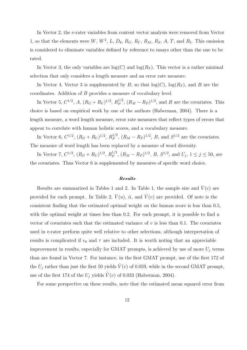
In Vector 2, the e-rater variables from content vector analysis were removed from Vector

1, so that the elements were W , W 2, L, D8, RG, RU , RM , RS, A, T , and B5. This omission

is considered to eliminate variables defined by reference to essays other than the one to be

rated.

In Vector 3, the only variables are log(C) and log(RT ). This vector is a rather minimal

selection that only considers a length measure and an error rate measure.

In Vector 4, Vector 3 is supplemented by B, so that log(C), log(RT ), and B are the

coordinates. Addition of B provides a measure of vocabulary level.

In Vector 5, C1/2, A, (RG + RU)1/2, R1/2P , (RM −RP )1/2, and B are the covariates. This

choice is based on empirical work by one of the authors (Haberman, 2004). There is a

length measure, a word length measure, error rate measures that reflect types of errors that

appear to correlate with human holistic scores, and a vocabulary measure.

In Vector 6, C1/2, (RG + RU)1/2, R1/2P , (RM − RP )1/2, B, and S1/2 are the covariates.

The measure of word length has been replaced by a measure of word diversity.

In Vector 7, C1/2, (RG + RU)1/2, R1/2P , (RM − RP )1/2, B, S1/2, and Uj, 1 ≤ j ≤ 50, are

the covariates. Thus Vector 6 is supplemented by measures of specific word choice.

Results

Results are summarized in Tables 1 and 2. In Table 1, the sample size and V (e) are

provided for each prompt. In Table 2, V (u), α, and V (v) are provided. Of note is the

consistent finding that the estimated optimal weight on the human score is less than 0.5,

with the optimal weight at times less than 0.2. For each prompt, it is possible to find a

vector of covariates such that the estimated variance of v is less than 0.1. The covariates

used in e-rater perform quite well relative to other selections, although interpretation of

results is complicated if e6 and τ are included. It is worth noting that an appreciable

improvement in results, especially for GMAT prompts, is achieved by use of more Uj terms

than are found in Vector 7. For instance, in the first GMAT prompt, use of the first 172 of

the Uj rather than just the first 50 yields V (v) of 0.059, while in the second GMAT prompt,

use of the first 174 of the Uj yields V (v) of 0.033 (Haberman, 2004).

For some perspective on these results, note that the estimated mean squared error from

12

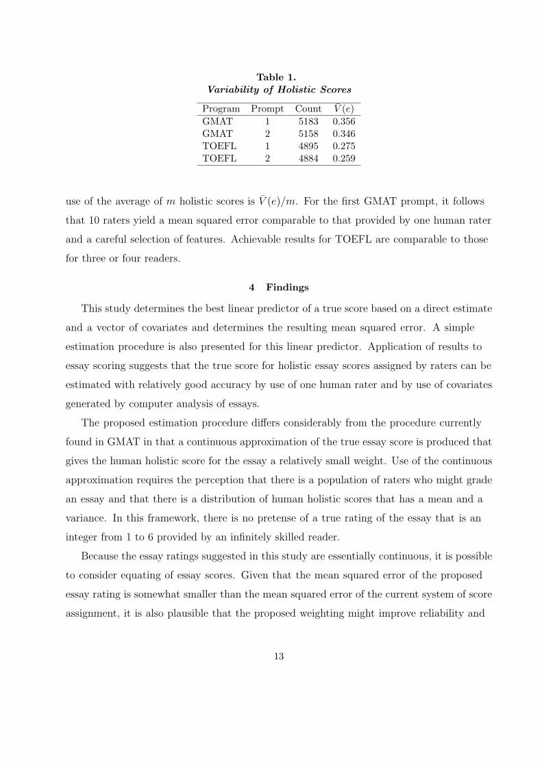
Table 1.Variability of Holistic Scores

Program Prompt Count V (e)GMAT 1 5183 0.356GMAT 2 5158 0.346TOEFL 1 4895 0.275TOEFL 2 4884 0.259

use of the average of m holistic scores is V (e)/m. For the first GMAT prompt, it follows

that 10 raters yield a mean squared error comparable to that provided by one human rater

and a careful selection of features. Achievable results for TOEFL are comparable to those

for three or four readers.

4 Findings

This study determines the best linear predictor of a true score based on a direct estimate

and a vector of covariates and determines the resulting mean squared error. A simple

estimation procedure is also presented for this linear predictor. Application of results to

essay scoring suggests that the true score for holistic essay scores assigned by raters can be

estimated with relatively good accuracy by use of one human rater and by use of covariates

generated by computer analysis of essays.

The proposed estimation procedure differs considerably from the procedure currently

found in GMAT in that a continuous approximation of the true essay score is produced that

gives the human holistic score for the essay a relatively small weight. Use of the continuous

approximation requires the perception that there is a population of raters who might grade

an essay and that there is a distribution of human holistic scores that has a mean and a

variance. In this framework, there is no pretense of a true rating of the essay that is an

integer from 1 to 6 provided by an infinitely skilled reader.

Because the essay ratings suggested in this study are essentially continuous, it is possible

to consider equating of essay scores. Given that the mean squared error of the proposed

essay rating is somewhat smaller than the mean squared error of the current system of score

assignment, it is also plausible that the proposed weighting might improve reliability and

13

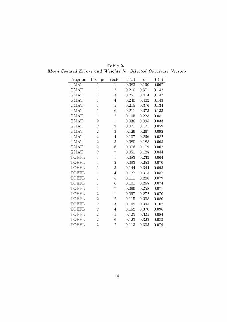
Table 2.Mean Squared Errors and Weights for Selected Covariate Vectors

Program Prompt Vector V (u) α V (v)GMAT 1 1 0.083 0.190 0.067GMAT 1 2 0.210 0.371 0.132GMAT 1 3 0.251 0.414 0.147GMAT 1 4 0.240 0.402 0.143GMAT 1 5 0.215 0.376 0.134GMAT 1 6 0.211 0.373 0.133GMAT 1 7 0.105 0.228 0.081GMAT 2 1 0.036 0.095 0.033GMAT 2 2 0.071 0.171 0.059GMAT 2 3 0.126 0.267 0.092GMAT 2 4 0.107 0.236 0.082GMAT 2 5 0.080 0.188 0.065GMAT 2 6 0.076 0.179 0.062GMAT 2 7 0.051 0.128 0.044TOEFL 1 1 0.083 0.232 0.064TOEFL 1 2 0.093 0.253 0.070TOEFL 1 3 0.144 0.344 0.095TOEFL 1 4 0.127 0.315 0.087TOEFL 1 5 0.111 0.288 0.079TOEFL 1 6 0.101 0.268 0.074TOEFL 1 7 0.096 0.258 0.071TOEFL 2 1 0.097 0.272 0.070TOEFL 2 2 0.115 0.308 0.080TOEFL 2 3 0.169 0.395 0.102TOEFL 2 4 0.152 0.370 0.096TOEFL 2 5 0.125 0.325 0.084TOEFL 2 6 0.123 0.322 0.083TOEFL 2 7 0.113 0.305 0.079

14

validity of essay scores; however, this possibility can only be verified with further research.

The proposed method of essay scoring has potential problems. It is not clear whether

the public can be persuaded that a reduced weight to human holistic scores is desirable, no

matter what statistical arguments may be made. Perhaps this potential concern can be

reduced by emphasizing that the essay features used by the computer analysis do provide

measures of writing quality that are strongly related to human holistic scores and that the

collection of human holistic scores of essay responses has been employed to determine the

final predictor of the essay score.

A further potential difficulty is that behavior of essay writers might change if they

are aware of the scoring procedure used to evaluate the essay. Exploiting this knowledge

might be difficult in practice, and, in any event, research concerning the relationship of

essay features to human holistic scores is publicly available, at least to a substantial extent

(Haberman, 2004).

In conclusion, it appears that the proposed regression-based method of essay assessment

should be seriously considered in those cases in which essays are available in

computer-readable form and in which human holistic scoring is employed.

15

References

Attali, Y., & Burstein, J. (2004). Automated essay scoring with e-rater v.2.0. Paper

presented at the Annual Conference of the International Association for Educational

Assessment (IAEA), Philadelphia, PA.

Bock, R. D., & Petersen, A. C. (1975). A multivariate correction for attenuation.

Biometrika, 62, 673–678.

Breland, H. M. (1996). Word frequency and word difficulty: A comparison of counts in

four corpora. Psychological science, 7, 96–99.

Breland, H. M., Jones, R. J., & Jenkins, L. (1994). The College Board vocabulary study

(College Board Rep. no. 94-4). Princeton, NJ: ETS.

Burstein, J., Chodorow, M., & Leacock, C. (in press). Automated essay evaluation: The

Criterion Online Service. AI Magazine, 25.

Gini, C. (1912). Variabilita e mutabilita: Contributo allo studio delle distribuzioni e delle

relazioni statische. Bologna, Italy: Cuppini.

Haberman, S. J. (2004). Statistical and measurement properties of features used in essay

assessment. Manuscript in preparation.

Holland, P. W., & Hoskens, M. (2003). Classical test theory as a first-order item response

theory: Application to true-score prediction from a possibly non-parallel test.

Psychometrika, 68.

Kelley, T. L. (1947). Fundamentals of statistics. Cambridge, MA: Harvard University

Press.

Lord, F. M., & Novick, M. R. (1968). Statistical theories of mental test scores. Reading,

MA: Addison-Wesley.

Qian, J., & Haberman, S. J. (2003). The best linear predictor for true score from a direct

estimate and a derived estimate. Paper presented at the annual Joint Statistical

Meetings of the American Statistical Association, San Francisco, CA.

Rao, C. R. (1973). Linear statistical inference and its applications. New York: John Wiley.

Simpson, E. H. (1949). The measurement of diversity. Nature, 163, 688.

16

I.N. 725881