Embed Size (px)
Citation preview

The Binomial Probability Distribution and Related Topics
Chapter 5
Understandable Statistics Ninth EditionBy Brase and Brase Prepared by Yixun ShiBloomsburg University of PennsylvaniaEdited by José Neville DíazUniversity of Puerto Rico at Aguadilla

Copyright © Houghton Mifflin Harcourt Publishing Company. All rights reserved. 5 | 2
Copyright © Houghton Mifflin Harcourt Publishing Company. All rights reserved. 5 | 3
Statistical Experiments and Random Variables
Statistical Experiments – any process by which measurements are obtained.
A quantitative variable, x, is a random variable if its value is determined by the outcome of a random experiment.
Random variables can be discrete or continuous

Copyright © Houghton Mifflin Harcourt Publishing Company. All rights reserved. 5 | 4
Random Variable
• In probability and statistics, a random variable is a variable whose value results from a measurement on some type of random process. Formally, it is a function.
Copyright © Houghton Mifflin Harcourt Publishing Company. All rights reserved. 5 | 5
• A Random Experiment is an experiment or observation that can be repeated numerous times under the same conditions.
• The outcome of an individual random experiment must be independent and identically distributed. It must in no way be affected by any previous outcome and cannot be predicted with certainty.
Copyright © Houghton Mifflin Harcourt Publishing Company. All rights reserved. 5 | 6
Independent and identically distributed (i.i.d.) Each random variable has the same probability distribution as the others and all are mutually independent.
Copyright © Houghton Mifflin Harcourt Publishing Company. All rights reserved. 5 | 7
Random Variables and Their Probability Distributions
• Discrete random variables – can take on only a countable or finite number of values.
• Continuous random variables – can take on countless values in an interval on the real line
• Probability distributions of random variables – An assignment of probabilities to the specific values or a range of values for a random variable.
Copyright © Houghton Mifflin Harcourt Publishing Company. All rights reserved. 5 | 8
• In probability theory and statistics, a probability distribution identifies either the probability of each value of a random variable (when the variable is discrete), or the probability of the value falling within a particular interval (when the variable is continuous).
• The probability distribution describes the range of
possible values that a random variable can attain and the probability that the value of the random variable is within any (measurable) subset of that range.
Copyright © Houghton Mifflin Harcourt Publishing Company. All rights reserved. 5 | 9
A random variable is a number that is derived from a random process. For example, suppose that we measure the rainfall in July in different cities. One city might have 1.5 inches, another city might have 0.8 inches, and so on. The amount of rainfall is a random variable.
The number of hits Pedro Martinez allows when he pitches in a game
The number of students in a class with birthdays in January
The score that you get when you take the SAT test.
Give some other examples of random variables. Think of some examples that are discrete and some examples that are continuous.
Copyright © Houghton Mifflin Harcourt Publishing Company. All rights reserved. 5 | 10
For continuous random variables, we talk about the probability distribution function. The probability distribution function pertains to intervals of a continuous random variable.
Copyright © Houghton Mifflin Harcourt Publishing Company. All rights reserved. 5 | 11
One example of important distribution function is the uniform distribution function. A random variable is uniformly distributed means that the probability of landing in a particular interval is equal to the size of that interval divided by the size of the entire distribution.
For example, consider a random variable that is uniformly distributed between 0 and 100. The entire distribution has a width of 100. The probability of landing between 0 and 10 is 10/100, or 0.1
Copyright © Houghton Mifflin Harcourt Publishing Company. All rights reserved. 5 | 12
Discrete Probability Distributions
• Each value of the random variable has an assigned probability.
• The sum of all the assigned probabilities must equal 1.
Copyright © Houghton Mifflin Harcourt Publishing Company. All rights reserved. 5 | 13
Probability Distribution Features
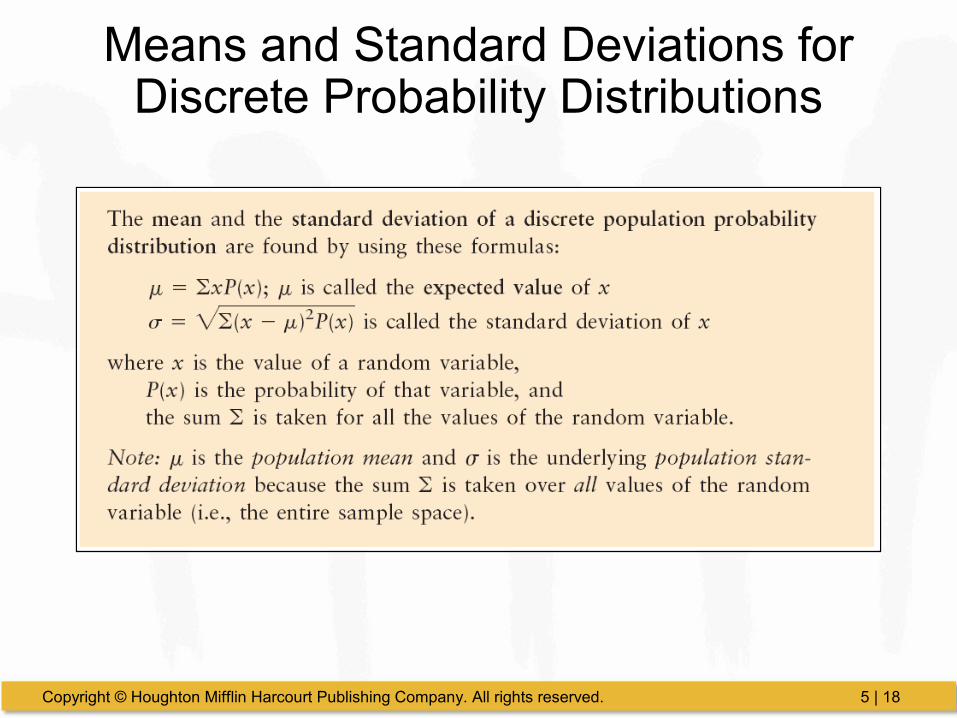
• Since a probability distribution can be thought of as a relative-frequency distribution for a very large n, we can find the mean and the standard deviation.
• When viewing the distribution in terms of the population, use µ for the mean and σ for the standard deviation.
Copyright © Houghton Mifflin Harcourt Publishing Company. All rights reserved. 5 | 14
Copyright © Houghton Mifflin Harcourt Publishing Company. All rights reserved. 5 | 15
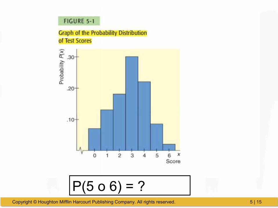
P(5 o 6) = ?
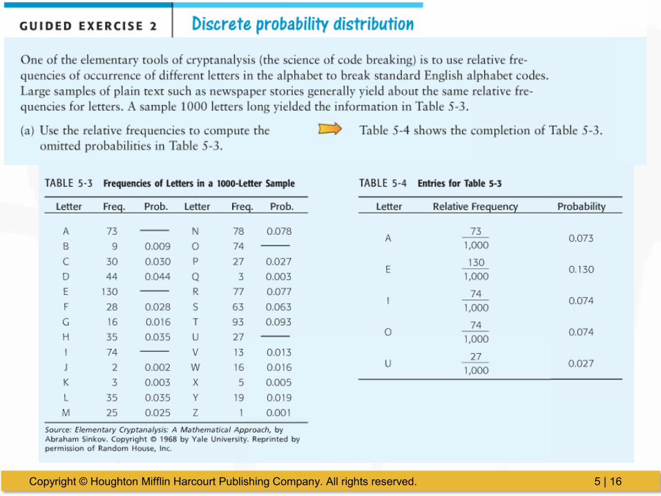
Copyright © Houghton Mifflin Harcourt Publishing Company. All rights reserved. 5 | 16
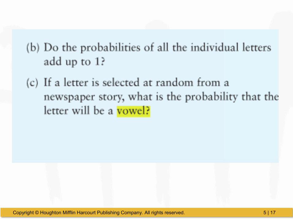
Copyright © Houghton Mifflin Harcourt Publishing Company. All rights reserved. 5 | 17
Copyright © Houghton Mifflin Harcourt Publishing Company. All rights reserved. 5 | 18
Means and Standard Deviations for Discrete Probability Distributions

Copyright © Houghton Mifflin Harcourt Publishing Company. All rights reserved. 5 | 19
Copyright © Houghton Mifflin Harcourt Publishing Company. All rights reserved. 5 | 20
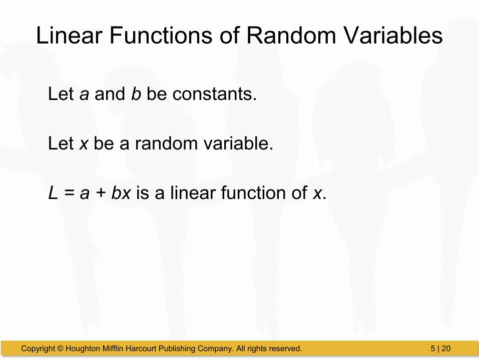
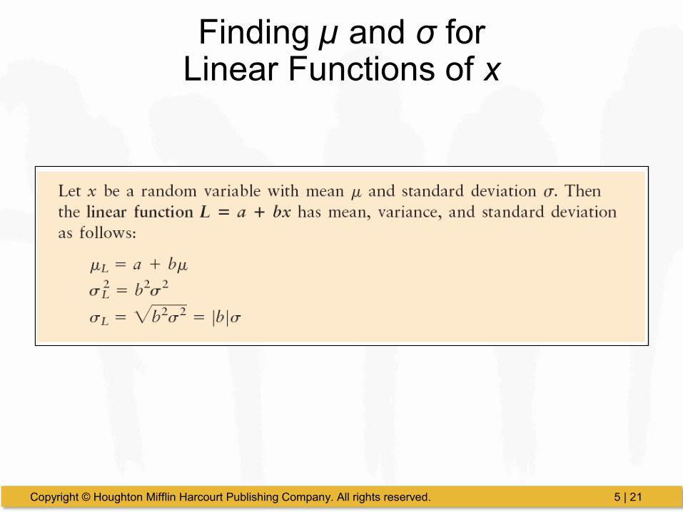
Linear Functions of Random Variables
Let a and b be constants.
Let x be a random variable.
L = a + bx is a linear function of x.
Copyright © Houghton Mifflin Harcourt Publishing Company. All rights reserved. 5 | 21
Finding µ and σ forLinear Functions of x
Copyright © Houghton Mifflin Harcourt Publishing Company. All rights reserved. 5 | 22
Independent Random Variables
Let x1 and x2 be random variables.Then the random variables are independent if any event of x1 is independent of any event of x2.
Copyright © Houghton Mifflin Harcourt Publishing Company. All rights reserved. 5 | 23
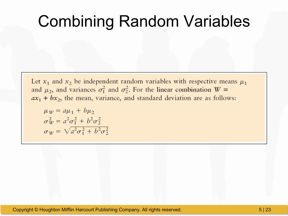
Combining Random Variables
Copyright © Houghton Mifflin Harcourt Publishing Company. All rights reserved. 5 | 24
Copyright © Houghton Mifflin Harcourt Publishing Company. All rights reserved. 5 | 25
Binomial Experiments
There are a fixed number of trials. This is denoted by n. The n trials are independent and repeated under identical conditions. Each trial has two outcomes:
S = success F = failure

Copyright © Houghton Mifflin Harcourt Publishing Company. All rights reserved. 5 | 26
Binomial Experiments
• For each trial, the probability of success, p, remains the same. Thus, the probability of failure is 1 – p = q.
• The central problem is to determine the probability of r successes out of n trials.
Copyright © Houghton Mifflin Harcourt Publishing Company. All rights reserved. 5 | 27
Determining Binomial Probabilities
• Use the Binomial Probability Formula.
• Use Table 3 of Appendix II.
• Use technology.
Copyright © Houghton Mifflin Harcourt Publishing Company. All rights reserved. 5 | 28
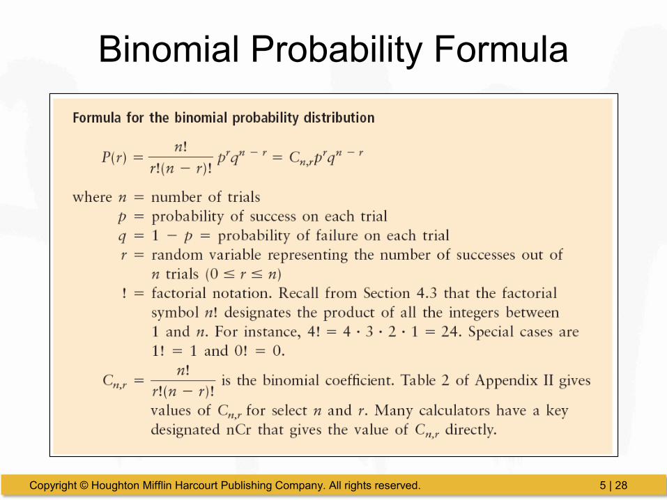
Binomial Probability Formula
Copyright © Houghton Mifflin Harcourt Publishing Company. All rights reserved. 5 | 29
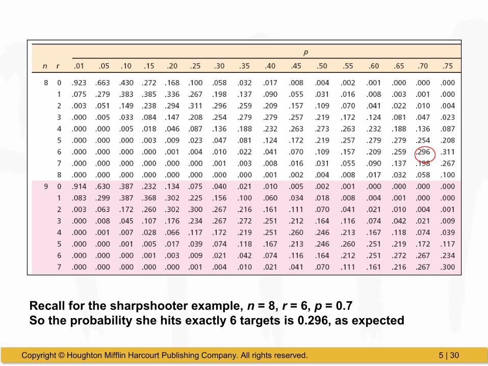
Using the Binomial Table
Locate the number of trials, n.
Locate the number of successes, r.
Follow that row to the right to the corresponding p column.
Copyright © Houghton Mifflin Harcourt Publishing Company. All rights reserved. 5 | 30
Recall for the sharpshooter example, n = 8, r = 6, p = 0.7So the probability she hits exactly 6 targets is 0.296, as expected
Copyright © Houghton Mifflin Harcourt Publishing Company. All rights reserved. 5 | 31
Binomial Probabilities
• At times, we will need to calculate other probabilities:– P(r < k)– P(r ≤ k)– P(r > k)– P(r ≥ k)
Where k is a specified value less than or equal to the number of trials, n.
Copyright © Houghton Mifflin Harcourt Publishing Company. All rights reserved. 5 | 32
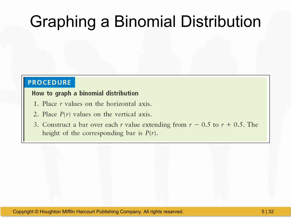
Graphing a Binomial Distribution
Copyright © Houghton Mifflin Harcourt Publishing Company. All rights reserved. 5 | 33
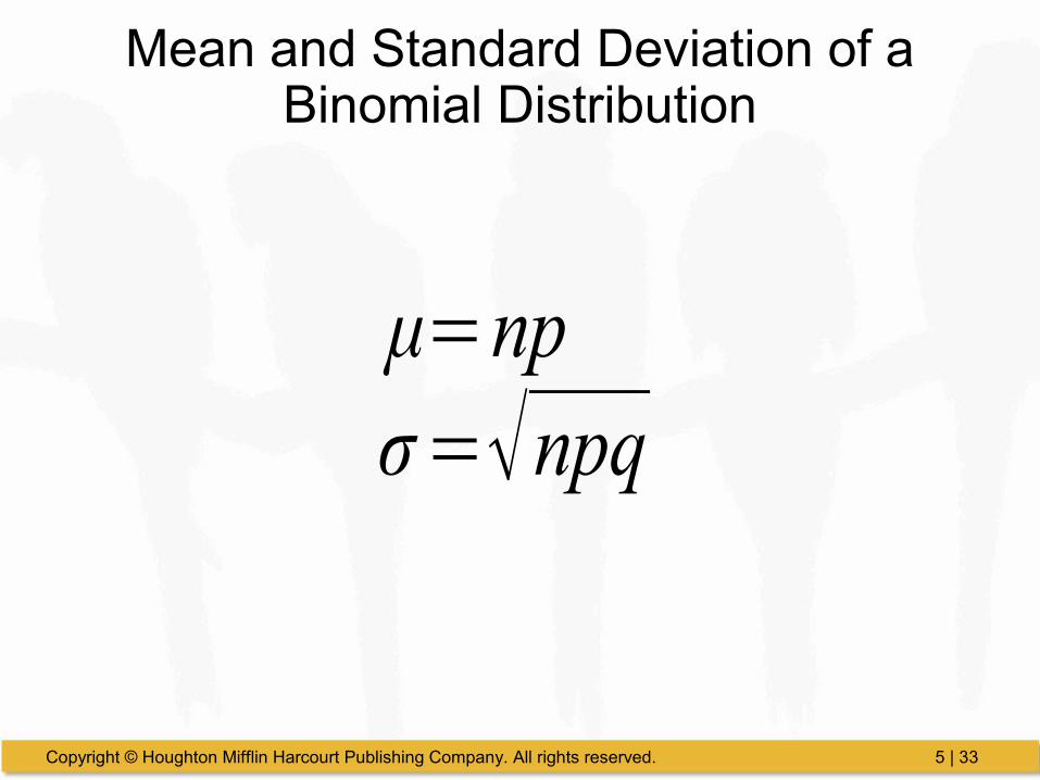
Mean and Standard Deviation of a Binomial Distribution
μ=npσ=√npq
Copyright © Houghton Mifflin Harcourt Publishing Company. All rights reserved. 5 | 34
Critical Thinking
• Unusual values – For a binomial distribution, it is unusual for the number of successes r to be more than 2.5 standard deviations from the mean.
– This can be used as an indicator to determine whether a specified number of r out of n trials in a binomial experiment is unusual.
Copyright © Houghton Mifflin Harcourt Publishing Company. All rights reserved. 5 | 35
Quota Problems
We can use the binomial distribution table “backwards” to solve for a minimum number of trials.In these cases, we know r and p
We use the table to find an n that satisfies our required probability
Copyright © Houghton Mifflin Harcourt Publishing Company. All rights reserved. 5 | 36
The Geometric Distribution
• Suppose that rather than repeat a fixed number of trials, we repeat the experiment until the first success.
• Examples:– Flip a coin until we observe the first head– Roll a die until we observe the first 5– Randomly select DVDs off a production line
until we find the first defective disk
Copyright © Houghton Mifflin Harcourt Publishing Company. All rights reserved. 5 | 37
Copyright © Houghton Mifflin Harcourt Publishing Company. All rights reserved. 5 | 38
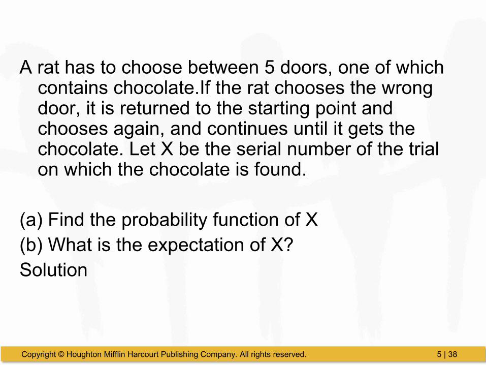
A rat has to choose between 5 doors, one of which contains chocolate.If the rat chooses the wrong door, it is returned to the starting point and chooses again, and continues until it gets the chocolate. Let X be the serial number of the trial on which the chocolate is found.
(a) Find the probability function of X(b) What is the expectation of X?Solution
Copyright © Houghton Mifflin Harcourt Publishing Company. All rights reserved. 5 | 39
The Poisson Distribution
This distribution is used to model the number of “rare” events that occur in a time interval, volume, area, length, etc…
Examples:Number of auto accidents during a monthNumber of diseased trees in an acreNumber of customers arriving at a bank
Copyright © Houghton Mifflin Harcourt Publishing Company. All rights reserved. 5 | 40
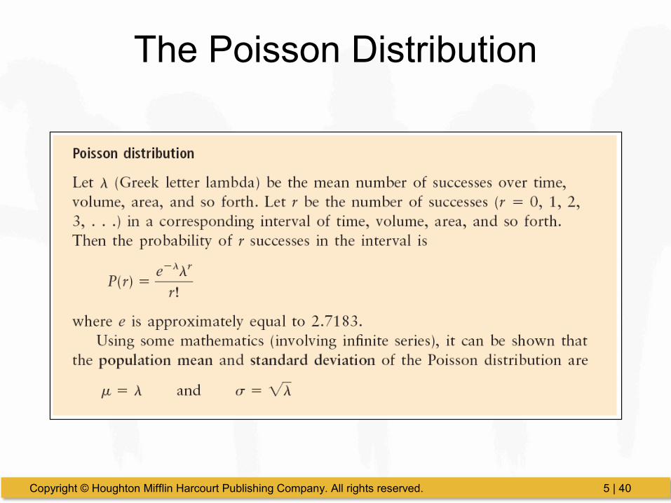
The Poisson Distribution
Copyright © Houghton Mifflin Harcourt Publishing Company. All rights reserved. 5 | 41
Finding Poisson ProbabilitiesUsing the Table
We can use Table 4 of Appendix II instead of the formula.
1) Find λ at the top of the table.2) Find r along the left margin of the table.
Copyright © Houghton Mifflin Harcourt Publishing Company. All rights reserved. 5 | 42
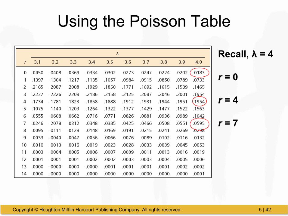
Using the Poisson Table
Recall, λ = 4
r = 0
r = 4
r = 7
Copyright © Houghton Mifflin Harcourt Publishing Company. All rights reserved. 5 | 43
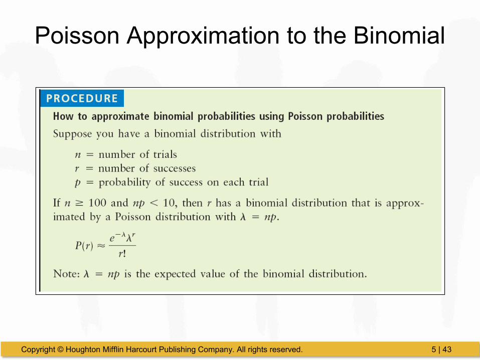
Poisson Approximation to the Binomial

Copyright © Houghton Mifflin Harcourt Publishing Company. All rights reserved. 5 | 44
Suppose the average number of lions seen on a 1-day safari is 5. What is the probability that tourists will see fewer
than four lions on the next 1-day safari? Solution: This is a Poisson experiment in which we know the
following:
Copyright © Houghton Mifflin Harcourt Publishing Company. All rights reserved. 5 | 45
Vehicles pass through a junction on a busy road at an average rate of 300 per hour.Find the probability that none passes in a given minute.What is the expected number passing in two minutes?Find the probability that this expected number actually pass
through in a given two-minute period.

Copyright © Houghton Mifflin Harcourt Publishing Company. All rights reserved. 5 | 46
Solution: Lamda =300/1hr Nuevo lamda=300/60=5 1mina) P(0)=.0067b) 5x2=10c) P(10)=.125
Copyright © Houghton Mifflin Harcourt Publishing Company. All rights reserved. 5 | 47
Binomial Approximation by PoissonA manufacturer of Christmas tree bulbs knows that
2% of its bulbs are defective. Approximate the probability that a box of 100 of these bulbs contains at most three defective bulbs. Assuming independence, we have binomial distribution with parameters p=0.02 and n=100.
The Poisson distribution with gives using the binomial distribution, we obtain, after some tedious calculations, Hence, in this case, the Poisson approximation is extremely close to the true value, but much easier to find.
Copyright © Houghton Mifflin Harcourt Publishing Company. All rights reserved. 5 | 48
A company makes electric motors. The probability an electric motor is defective is 0.01. What is the probability that a sample of 300 electric motors will contain exactly 5 defective motors?