The Brewer-Dobsoncirculation in CMIP6

The Brewer-Dobson circulation in CMIP6Marta Abalos1, Natalia Calvo1, Samuel Benito-Barca1, Hella Garny2, Steven C. Hardiman3, Pu Lin4,5,Martin B. Andrews6, Neal Butchart6, Rolando Garcia7, Clara Orbe8, David Saint-Martin9,Shingo Watanabe10, and Kohei Yoshida11

1Universidad Complutense de Madrid, Madrid, Spain2Deutsches Zentrum für Luft- und Raumfahrt (DLR), Oberpfaffenhofen, Germany3Met Office, Exeter, United Kingdom4NOAA/Geophysical Fluid Dynamics Laboratory, Princeton, NJ, USA5Program in Atmospheric and Oceanic Sciences, Princeton University, Princeton, NJ, USA6Met Office Hadley Centre, Exeter, UK7National Center for Atmospheric Research, Boulder, CO, USA8NASA Goddard Institute for Space Studies, New York, NY, USA9Centre National de Recherches Météorologiques, Toulouse, France10Japan Agency for Marine-Earth Science and Technology (JAMSTEC), Yokohama, Japan11Meteorological Research Institute, Tsukuba, Japan

Correspondence: Marta Abalos ([email protected])

Abstract. The Brewer-Dobson circulation (BDC) is a key feature of the stratosphere that models need to accurately represent in

order to improve the representation of surface climate variability. For the first time, the Climate Model Intercomparison Project

includes in its phase 6 (CMIP6) a set of diagnostics that allow for careful evaluation of the BDC. Here, the BDC is evaluated

against observations and reanalyses using historical simulations. CMIP6 results confirm the well-known inconsistency in BDC

trends between observations and models in the middle and upper stratosphere. The increasing CO2 simulations feature a robust5

acceleration of the BDC but also reveal large uncertainties in the deep branch trends. The very close connection between the

shallow branch and surface temperature is highlighted, which is absent in the deep branch. The trends in mean age of air

are shown to be more robust throughout the stratosphere than those in the residual circulation. The paper reflects the current

knowledge and main uncertainties regarding the BDC.

1 Introduction

The Brewer-Dobson circulation (BDC) describes the net transport of heat and tracers in the stratosphere, and therefore plays

a primary role in its chemical composition and radiative transfer properties (Butchart, 2014). In particular, the strength of the

BDC controls key features such as the rate of stratospheric ozone recovery (WMO, 2018), the stratosphere-to-troposphere

exchange of ozone (e.g. Albers et al., 2018), and the amount of water vapor entering the stratosphere (Randel and Park, 2019).15

The BDC is also fundamentally connected with the thermal structure of the stratosphere and in particular the static stability

1

10

https://doi.org/10.5194/acp-2021-206Preprint. Discussion started: 29 March 2021c© Author(s) 2021. CC BY 4.0 License.

around the tropopause (Birner, 2010), a key radiative forcing region that also influences deep convection (e.g. Emanuel et al.,

2013). Therefore, realistically representing the BDC strength and its variability is a key target for climate models.

The BDC is commonly separated into two components: the residual circulation, which is the mean meridional mass circu-

lation approximating the zonal-mean lagrangian transport, and two-way mixing, which accounts for zonal asymmetries and20

irreversible tracer transport caused by stirring of air masses following wave dissipation (Plumb, 2002). The residual circu-

lation in turn is typically divided into the shallow and the deep branch, with the former approximately limited to latitudes

below 50◦N/S and levels below 50 hPa and overturning timescales under 1 year (Birner and Bönisch, 2011). In the literature,

the term BDC sometimes refers to the residual circulation alone, and previous multi-model assessments of the BDC focused

on this component (i.e. Butchart et al., 2010; Hardiman et al., 2014). However, there is growing evidence over the last years25

of the important role of mixing for the net tracer stratospheric transport strength (Garny et al., 2014; Dietmüller et al., 2017;

Eichinger et al., 2018; Ploeger et al., 2015). The mean age of air (AoA) is a transport diagnostic that informs on the elapsed

time since an air parcel entered the stratosphere, and it can be estimated from observations of long-lived tracers such as SF6

or CO2 (e.g. Engel et al., 2017). Therefore, it integrates the effect of both residual circulation and mixing. While there are no

direct measurements of the BDC strength, model results can be evaluated against observational estimates of the AoA.30

In this study we assess the climatology and trends in the BDC in CMIP6 models, with a focus on current open questions.

A key open question is the disagreement between observations and models regarding the past BDC trends. While models

consistently predict a reduction in AoA mainly due to an acceleration of the residual circulation (Li et al., 2018), the longest

observational estimates produce non-significant slightly positive trends (Engel et al., 2017). Various studies over the last years

suggest that an acceleration of the BDC might actually be observed in the lower stratosphere (see WMO (2018) and references35

therein). Moreover, it has been argued that the formation of the ozone hole has had a significant impact on the past BDC

acceleration until the end of the 20th century (Oman et al., 2009; Li et al., 2018; Polvani et al., 2018; Abalos et al., 2019).

However, the observation-model discrepancy remains at higher altitudes. Indeed, the trends in the deep branch and its drivers

remain more uncertain (WMO, 2018), given the limitations of model top and the importance of parameterized gravity waves in

the upper stratosphere and mesosphere. On the other hand, recent work has highlighted that the observational AoA estimates40

are likely biased high (Fritsch et al., 2020).

CMIP6 is the first CMIP activity providing Transformed Eulerian Mean (TEM) data as model output (Gerber and Manzini,

2016). This allows for a more detailed analysis based on a consistent set of diagnostics as compared to previous assessments

(e.g. Manzini et al., 2014; Hardiman et al., 2014). Here, we use this TEM output to evaluate the past climatology and trends

in the BDC against reanalyses and observations using historical simulations, and to assess the BDC response to a 1%/year45

CO2 increase. In Section 2 we describe the CMIP6 models and simulations used, as well as other datasets employed. Section 3

analyzes the BDC in historical simulations, Section 4 examines the BDC changes associated with increases in CO2 and Section

5 explores the connections between BDC and surface warming. The main conclusions are summarized in the last Section.

2


Table 1. List of CMIP6 models with TEM and/or AoA diagnostics used in this study. AoA is only provided in the historical runs for MRI.

Model Model and data references Levels Model top TEM AoA

CNRM-ESM2-1 Séférian et al. (2019); Seferian (2018a, b) 91 78.4 km (∼ 0.01 hPa) ✗ XCESM2-WACCM Gettelman et al. (2019); Danabasoglu (2019a, b) 70 0.0000045 hPa X ✗

MIROC6 Tatebe et al. (2019); Tatebe and Watanabe (2018a, b) 81 0.004 hPa X ✗

GFDL-ESM4 Dunne et al. (2020); Krasting et al. (2018a, b) 49 0.01 hPa X XGISS-E2-2-G Rind et al. (2020); Orbe et al. (2020); NASA/GISS (2019) 102 0.002 hPa X XUKESM-1-0-LL Sellar et al. (2019); Tang et al. (2019a, b) 85 85 km (∼ 0.005 hPa) X XHadGEM3-GC31-LL Williams et al. (2018); Ridley et al. (2019a, b) 85 85 km (∼ 0.005 hPa) X ✗

MRI-ESM2-0 Yukimoto et al. (2019a, b, c) 80 0.01 hPa X X(historical)

2 Data and Methods

CMIP6 models providing the necessary TEM output, as described in Gerber and Manzini (2016), have been used. We refer50

to that paper for the specific diagnostic description. In addition to the TEM diagnostics, some models additionally provided

mean age of air (AoA). Table 1 shows the models used, their number of levels, the model top and the corresponding available

variables. While each model has a different horizontal resolution (not shown), they are all in the range between 1 and 2 degrees

in longitude and latitude. Note that two more models output TEM variables, CESM2 and Can-ESM5, but we did not include

them in the analyses because they have low model tops (2.25 hPa and 1 hPa, respectively), and did not represent the residual55

circulation structure adequately (not shown).

Model results have been compared to reanalysis over the historical period. Because there is a large spread in the BDC values

obtained from reanalyses (Abalos et al., 2015), we used three reanalyses: ERA-Interim (Interim European Centre for Medium-

Range Weather forecasts Reanalysis, Dee et al. (2011)), JRA-55 (Japanese 55 year Reanalysis, Kobayashi et al. (2015)), and60

MERRA (Modern-Era Retrospective Analysis for Research and Applications, Rienecker et al. (2011)). We have used the resid-

ual circulation for these three reanalyses from Abalos et al. (2015), which covers the period 1979-2012. In order to com-

pare AoA with observational estimates, we used AoA derived from the Michelson Interferometer MIPAS (Stiller et al., 2012;

Haenel et al., 2015). Here, we use a new version of AoA derived from an updated retrieval of SF6 (Stiller et al., 2020). Fur-

thermore, AoA derived from GOZCARDS N2O data is used (Linz et al., 2016), as well as AoA data derived from in-situ65

measurements of CO2 and SF6 by Engel et al. (2017) and Andrews et al. (2001).

The model simulations used are historical and 1pctCO2. We consider one member of each simulation, except for Figures 5

and 6, where all available members from the historical simulations are used (5 for CRNM-ESM2-1, 3 for CESM2-WACCM, 1

for GFDL-ESM4, 4 for GISS-E2-2-G, 4 for HadGEM3-GC31-LL, 1 for MIROC6, 5 for MRI-ESM2-0-LL, 18 for UKESM1-0-

LL). The fully-coupled (DECK) historical simulations cover the period 1850 to 2014, with observed emissions of greenhouse70

3


gases and other external forcings, and will be used to examine past climatology and trends and compare to observations or

reanalysis when possible. For comparison purposes we have focused on the period 1975-2014. Note that this period encom-

passess the reanalysis period considered (1979-2012), but it is slightly longer. This is done to enhance statistical significance

trend calculations for model output. The small difference in the period considered is assumed to have a negligible impact on the

climatological BDC. The 1pctCO2 simulations are initialized from preindustrial (1850) conditions and are 150 years long, with75

CO2 concentrations increasing gradually at a 1%/year rate (Eyring et al., 2016). In order to establish statistical significance

we have used a two-tailed Student t test at the 95% confidence level. We consider there is intermodel agreement if 66% of the

models are consistent.

3 Representation of the BDC in CMIP6 historical simulations

This section aims to assess the degree of agreement in the BDC climatology and trends between CMIP6 historical simulations80

and observations or reanalysis data.

3.1 Climatology and seasonality

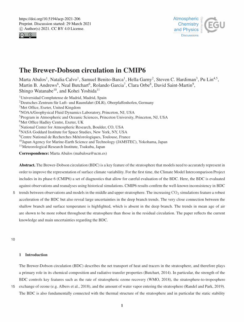
Figure 1 shows the climatological structure of the residual circulation in the CMIP6 multimodel mean (MMM, panel b) com-

pared with the multi-reanalysis mean (panel a). The climatological structure and magnitude are overall very similar in both

datasets. Both models and reanalyses highlight a minimum in tropical upwelling at ∼ 50 hPa of about 0.2 mm · s−1, and a85

maximum at ∼ 1.5–2 hPa of about 1.2 mm · s−1. The annual mean residual circulation structure in Fig. 1 is consistent with

previous model intercomparison studies such as CMIP5 (Hardiman et al., 2014).

In order to examine the quantitative differences in more detail, the tropical upwelling mass flux is examined. This is computed

as the net upwelling between the annual mean turnaround latitudes (i.e., the latitudes separating the upwelling and downwelling

regions). The calculation is based on the streamfunction, which in turn is computed from the meridional component of the90

residual circulation provided as model output, v̄∗. The streamfunction is obtained as

Ψ̄∗(φ,p) =−cosφ

g

0∫

p

v̄∗dp′ (1)

where p is pressure, φ is latitude, g the gravitational constant on Earth, and it is assumed that v̄∗ tends to zero as p→ 0. The

upwelling mass flux is then computed at each level as

M(p) = 2πa(Ψ̄∗

max(p)− Ψ̄∗min(p)

)(2)95

where Ψ̄∗max and Ψ̄∗

min are the maximum and minimum values of the residual streamfunction at each pressure level, which

correspond to the northern and southern turnaround latitudes, respectively (Rosenlof, 1995).

4


0.1

0.1

0.5

0.5

0.5

1

1

11

5

5

5

5

10

10

10

50

-50

-10

-10

-10

-5

-5

-5

-5

-1

-1

-1-1

-0.5

-0.5

-0.5

-0.5

-0.1

-0.1

-0.1

-60 -30 0 30 60

Latitude

100

101

102

Pre

ssure

(hP

a)

0.1

0.5

0.5

1

1

1

5

5

5

10

10

50

-50

-10-1

0

-5

-5

-5

-1-1

-0.5

-0.5

-0.1

(a) (b)

-60 -30 0 30 60

Latitude

100

101

102

Pre

ssure

(hP

a)

-3 -2.4 -1.8 -1.2 -0.6 0 0.6 1.2 1.8 2.4 3

mm s-1

MRM 1979-2012 MMM 1975-2014

Figure 1. Annual mean climatology for the multi reanalysis mean (a) and multi model mean for the historical simulations (b) of the vertical

component of the residual circulation (w̄∗, in mm ·s−1, shading) and residual streamfunction (Ψ∗, in kg ·m−1 ·s−1, contours). Black thick

contours indicate the location of the turnaround latitudes. The red contour in the right panel shows the turnaround latitudes for reanalyses.

Black dots represent regions where there is disagreement in the sign of w̄∗ for more than 66% (2/3) of the individual reanalyses or models

(which happens only around turnaround latitudes).

Figure 2 shows the seasonality in the tropical upwelling mass flux for the lower (70 hPa) and upper (1.5 hPa) stratosphere,

representative of the shallow and deep branches, respectively. Note that, while the level of 70 hPa is commonly used to represent

the shallow branch, 1.5 hPa is higher than usually considered for the deep branch. We argue that this level is optimal for the100

characterization of the deep branch, since tropical upwelling maximizes at this level in the upper stratosphere (Fig. 1). All

models show a generally consistent seasonality, with an annual cycle peaking in November-December in the shallow branch,

and an amplitude of about 50% of the climatological mean, and a semi-annual cycle peaking in June and December for the

deep branch, with an amplitude of about 80%. The seasonality is consistent with that of reanalyses, and the intermodel spread

is of similar magnitude to the reanalysis spread. In particular, the intermodel spread is over 40% of the climatological mean105

for the lower stratosphere and over 30% for the upper stratosphere. The annual cycle in the lower stratosphere has been

linked to seasonality of wave forcing in the extratropics, subtropics and tropics (e.g. Randel et al., 2008; Ueyama et al., 2013;

Ortland and Alexander, 2014; Kim et al., 2016). The semi-annual cycle in the upper stratosphere has been less studied, and

is probably linked to the combined annual cycles of the downwelling in each hemisphere and to the secondary circulation

associated with the Semi-Annual Oscillation (e.g. Garcia et al., 1997; Young et al., 2011).110

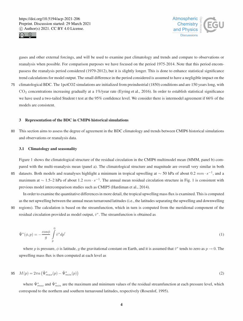
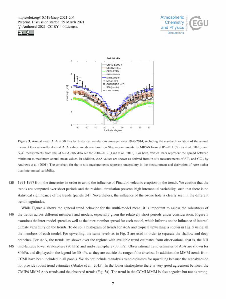
As mentioned in the Introduction, the mean age of air provides an estimate of the net transport circulation strength that can be

compared to observational estimates. Figure 3 shows the AoA climatology at 50 hPa for the models that provide this quantity

(see Table 1), together with the observational estimates described in Section 2. The simulated AoA values show considerable

spread across models, as previously shown for Chemistry-Climate Model Intercomparison project (CCMI) simulations (e.g.,

Dietmüller et al., 2017). The global mean age values vary by a factor of 2, between 2.5 and 5 years approximately. Nevertheless,115

5


JanFeb

Mar

AprM

ayJun

JulAug

SepOct

Nov

Dec

Month

2

3

4

5

6

7

8

9

10

10

9kg/s

(a)

JanFeb

Mar

AprM

ayJun

JulAug

SepOct

Nov

Dec

Month

0.2

0.4

0.6

0.8

1

1.2

1.4

10

9kg/s

(b)

GFDL-ESM4 CESM2-WACCM MIROC6 GISS-E2-2-G UKESM1-0-LL

HadGEM3-GC31-LL MRI-ESM2-0 JRA55 MERRA

Upwelling mass flux 70 hPa Upwelling mass flux 1.5 hPa

ERA-I

Figure 2. Seasonal cycle of tropical upwelling mass flux in the lower stratosphere (70 hPa, a) and in the upper stratosphere (1.5 hPa, b). Solid

color lines show models and dashed black lines show reanalyses.

the spread is within the large observational uncertainty. Note that the relationship between AoA and residual circulation strength

is not straightforward. For example, the GFDL model features a weak upwelling, but the AoA is relatively young. In contrast,

MRI has strong upwelling, but the AoA is the oldest. This lack of correspondence emphasizes the important role of mixing,

including subgrid effects, in determining the net transport strength (Garny et al., 2014; Dietmüller et al., 2017). The tropical

leaky pipe model relates the net upwelling through an isentrope with the mass flux-weighted tropics/extratropics gradient in120

AoA (e.g. Linz et al., 2016).

3.2 Past trends

In this section we examine the BDC trends over the historical period, in particular over the last four decades. Figure 4 shows the

multi-model mean trends in AoA (panel a) and upwelling (panel d) over the period 1975-2014. The AoA trends are negative

everywhere with values around -0.1 years/decade, with trends in the lower stratosphere larger in the Southern Hemisphere125

(SH) than in the Northern Hemisphere (NH). Consistently, the residual circulation accelerates throughout the stratosphere,

with enhanced tropical upwelling and polar downwelling, strongest in the SH. Note that there is also reduced downwelling

in midlatitudes in both hemispheres. The larger BDC polar downwelling trends in the SH are consistent with recent results

using CCMI models, and reflect the contribution of ozone depletion in the Antarctic lower stratosphere to the BDC trends

(Polvani et al., 2018, 2019; Abalos et al., 2019). In order to better capture this signal, the trends are shown separately for the130

end of the 20th century, a period of severe ozone depletion (panels b and e), and the beginning of the 21st century, when

ozone depletion stops and its recovery starts (panels c and f). It is clear that the BDC trends are stronger during the ozone hole

formation, particularly in the SH. The AoA trends for 1975-1990 are significantly different from those for 1998-2014 in the SH

lower stratosphere and in the NH above 30 hPa and north of about 40◦N (not shown). Note that we have excluded the period

6


-80 -60 -40 -20 0 20 40 60 800

2

4

6

8

10

Latitude (degree)

meanage [

yrs

]

AoA 50 hPa

CNRM-ESM2-1

UKESM1-0-LL

GFDL-ESM4

GISS-E2-2-G

MRI-ESM2-0

MIPAS SF6

GOZCARDS N2O

SF6 (in-situ)

CO2 (in-situ)

Figure 3. Annual mean AoA at 50 hPa for historical simulations averaged over 1990-2014, including the standard deviation of the annual

means. Observationally derived AoA values are shown based on SF6 measurements by MIPAS from 2005-2011 (Stiller et al., 2020), and

N2O measurments from the GOZCARDS data set for 2004-2012 (Linz et al., 2016). For both, vertical bars represent the spread between

minimum to maximum annual mean values. In addition, AoA values are shown as derived from in-situ measurements of SF6 and CO2 by

Andrews et al. (2001). The errorbars for the in-situ measurements represent uncertainty in the measurement and derivation of AoA rather

than interannual variability.

1991-1997 from the timeseries in order to avoid the influence of Pinatubo volcanic eruption on the trends. We caution that the135

trends are computed over short periods and the residual circulation presents high interannual variability, such that there is no

statistical significance of the trends (panels d-f). Nevertheless, the influence of the ozone hole is clearly seen in the different

trend magnitudes.

While Figure 4 shows the general trend behavior for the multi-model mean, it is important to assess the robustness of

the trends across different members and models, especially given the relatively short periods under consideration. Figure 5140

examines the inter-model spread as well as the inter-member spread for each model, which informs on the influence of internal

climate variability on the trends. To do so, a histogram of trends for AoA and tropical upwelling is shown in Fig. 5 using all

the members of each model. For upwelling, the same levels as in Fig. 2 are used in order to separate the shallow and deep

branches. For AoA, the trends are shown over the regions with available trend estimates from observations, that is, the NH

mid-latitude lower stratosphere (80 hPa) and mid-stratosphere (30 hPa). Observational trend estimates of AoA are shown for145

80 hPa, and displayed in the legend for 30 hPa, as they are outside the range of the abscissa. In addition, the MMM trends from

CCMI have been included in all panels. We do not include reanalysis trend estimates for upwelling because the reanalyses do

not provide robust trend estimates (Abalos et al., 2015). In the lower stratosphere there is very good agreement between the

CMIP6 MMM AoA trends and the observed trends (Fig. 5a). The trend in the CCMI MMM is also negative but not as strong.

7


80 60 40 20 0 20 40 60 80

Latitude

100

101

102

Pre

ssure

[hPa]

Trend in meanage (yrs/decade), MMM, historical years 1998-2014

80 60 40 20 0 20 40 60 80

Latitude

100

101

102

Pre

ssure

[hPa]

Trend in meanage (yrs/decade), MMM, historical years 1975-1990

0.24 0.18 0.12 0.06 0.00 0.06 0.12 0.18 0.24

yrs/dec

80 60 40 20 0 20 40 60 80

Latitude

100

101

102

Pre

ssure

[hPa]

Trend in meanage (yrs/decade), MMM, historical years 1975-2014(a) (b) (c)

(d) (e) (f)

Figure 4. Multimodel mean linear trend in AoA (top panels, years/decade) and w̄∗ (bottom panels, in mm · s−1 ·decade−1) from historical

simulations in shading over years 1975-2014 (a and d) 1975-1990 (b and e) and 1998-2014 (c and f). In top panels the contours show the

climatological AoA (years, contour interval 1 year). In the bottom panels the red contours show the turnaround latitudes averaged over each

corresponding period. Stippling in the top panels indicates statistically insignificant trends obtained with a Student’s t test at 95% confidence

level for more than 66% of the models. The trends for w̄∗ in the bottom panels are statistically insignificant everywhere for the three periods.

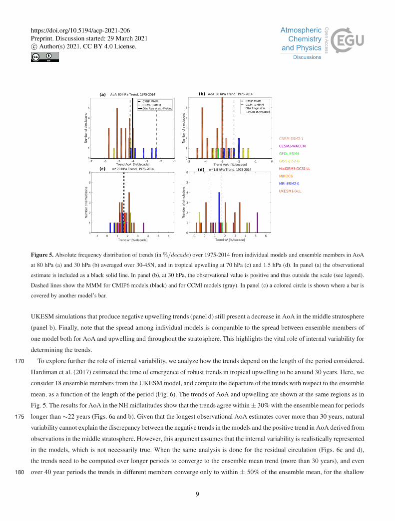
Note, however, the reduced number of models with AoA output in CMIP6. In the middle stratosphere (Fig. 5b) the MMM of150

both intercomparison projects produce a negative mean age trend between -2 and -3 %/decade, stronger for CMIP6. These

values disagree strongly with the observed estimate of +3 %/decade, even when taking the large uncertainty into account.

Even if one considers the updated estimate of AoA trends by Fritsch et al. (2020) of +1.5 ±3%/decade, the range of model

estimates barely overlaps with the observational uncertainty range. The residual circulation trends in the shallow branch (Fig.

5c) range from 0.5 to 3.5 %/decade, with a maximum in the distribution slightly below 2 %/decade, consistent with previous155

climate model simulations. The CMIP6 MMM trend is in excellent agreement with that from the CCMI MMM (Fig. 5c). In the

middle stratosphere, the value of the CMIP6 MMM trend is similar to that in the shallow branch (slightly below 2%/decade),

while the trend in the CCMI MMM is weaker (Fig. 5d).

When looking at individual simulations, the AoA trends show a similar spread in the trends across simulations of less than

3 %/decade at the two levels. In contrast, the residual circulation trends show a larger spread in the deep branch than in the160

shallow branch. In fact, some members feature slightly negative trends (ranging from -0.5 to over 5 %/decade) in the deep

branch upwelling. Therefore, a deceleration of the deep branch over 1975-2014 is compatible with the internal variability

in some of the CMIP6 models (although in the tail of the distribution), which could be consistent with observational AoA

estimates. Nevertheless, we note that negative upwelling trends do not necessarily imply positive AoA trends, because the

latter is an integrated quantity, affected non-locally by both advection and mixing (e.g. Garny et al., 2014). Indeed, the GISS and165

8


-5 -4 -3 -2 -1 00

1

2

3

4

5

Trend AoA [%/decade]

Num

ber

of sim

ula

tions

AoA 30 hPa Trend, 1975-2014

CMIP MMM

CCMI-1 MMM

Obs Engel et al:

+3% [0.15 yrs/dec]

CNRM-ESM2-1

CESM2-WACCM

GFDL-ESM4

GISS-E2-2-G

HadGEM3-GC31-LL

MIROC6

MRI-ESM2-0

UKESM1-0-LL

(a) (b)

(d)(c)

-7 -6 -5 -4 -3 -2 -10

1

2

3

4

5

Trend AoA [%/decade]

Num

ber

of sim

ula

tions

AoA 80 hPa Trend, 1975-2014

CMIP MMM

CCMI-1 MMM

Obs Ray et al: -4%/dec

-1 0 1 2 3 4 5 6

Trend w* [%/decade]

0

1

2

3

4

5

6

Num

ber of sim

ula

tions

w* 1.5 hPa Trend, 1975-2014w* 70 hPa Trend, 1975-2014

-1 0 1 2 3 4 5 6

Trend w* [%/decade]

0

1

2

3

4

5

6

Num

ber

of sim

ula

tions

Figure 5. Absolute frequency distribution of trends (in %/decade) over 1975-2014 from individual models and ensemble members in AoA

at 80 hPa (a) and 30 hPa (b) averaged over 30-45N, and in tropical upwelling at 70 hPa (c) and 1.5 hPa (d). In panel (a) the observational

estimate is included as a black solid line. In panel (b), at 30 hPa, the observational value is positive and thus outside the scale (see legend).

Dashed lines show the MMM for CMIP6 models (black) and for CCMI models (gray). In panel (c) a colored circle is shown where a bar is

covered by another model’s bar.

UKESM simulations that produce negative upwelling trends (panel d) still present a decrease in AoA in the middle stratosphere

(panel b). Finally, note that the spread among individual models is comparable to the spread between ensemble members of

one model both for AoA and upwelling and throughout the stratosphere. This highlights the vital role of internal variability for

determining the trends.

To explore further the role of internal variability, we analyze how the trends depend on the length of the period considered.170

Hardiman et al. (2017) estimated the time of emergence of robust trends in tropical upwelling to be around 30 years. Here, we

consider 18 ensemble members from the UKESM model, and compute the departure of the trends with respect to the ensemble

mean, as a function of the length of the period (Fig. 6). The trends of AoA and upwelling are shown at the same regions as in

Fig. 5. The results for AoA in the NH midlatitudes show that the trends agree within± 30% with the ensemble mean for periods

longer than ∼22 years (Figs. 6a and b). Given that the longest observational AoA estimates cover more than 30 years, natural175

variability cannot explain the discrepancy between the negative trends in the models and the positive trend in AoA derived from

observations in the middle stratosphere. However, this argument assumes that the internal variability is realistically represented

in the models, which is not necessarily true. When the same analysis is done for the residual circulation (Figs. 6c and d),

the trends need to be computed over longer periods to converge to the ensemble mean trend (more than 30 years), and even

over 40 year periods the trends in different members converge only to within ± 50% of the ensemble mean, for the shallow180

9


10 15 20 25 30 35 40-1.5

-1.2

-0.9

-0.6

-0.3

0

0.3

0.6

0.9

1.2

1.5

Number of years

Rela

tive d

evia

tion

AoA 30 hPa Trend

10 15 20 25 30 35 40-1.5

-1.2

-0.9

-0.6

-0.3

0

0.3

0.6

0.9

1.2

1.5

Number of years

Rela

tive d

evia

tion

AoA 80 hPa Trend(a) (b)

10 15 20 25 30 35 40

Number of years

-10

-8

-6

-4

-2

0

2

4

6

8

10

Re

lative

de

via

tio

n

w* 1.5 hPa Trend

10 15 20 25 30 35 40

Number of years

-2.5

-2

-1.5

-1

-0.5

0

0.5

1

1.5

2

2.5

Re

lative

de

via

tio

n

w* 70 hPa Trend(c) (d)

Figure 6. Trends from 18 ensemble members of UKESM1-0-LL for periods of increasing length (x-axis), ranging from 11 years (1975-1985)

to 40 years (1975-2014). Trends of individual ensemble members (crosses) are displayed as relative deviations from the ensemble mean trend.

(a) and (b) show trends in AoA and (c) and (d) show trends in upwelling, both variables at the same regions as in Fig. 5. Horizontal dashed

lines mark fixed values to ease comparison across panels.

branch (panel c), and to within ± 200% in the deep branch (panel d). At 10 hPa the 40-year trends show a± 150% spread (not

shown). These results highlight the substantially larger internal variability in the deep branch than the shallow branch of the

residual circulation, and show that trends in AoA converge more rapidly to the MMM than those in upwelling. This is due to

the memory of AoA, being an integrated quantity.

4 BDC response to CO2 increase185

In this section we examine the BDC trends and wave forcing in the 1pctCO2 simulations.

4.1 BDC trends

Figure 7 shows the trend in w̄∗ for the 1pctCO2 simulations in the different models and for the MMM. This figure clearly

demonstrates the increasing strength of the residual circulation due to CO2 increase, in both the deep and shallow branches.

The trend is particularly strong in the lower stratosphere and near the stratopause, mirroring the climatological structure (Fig. 1).190

Changes in the turnaround latitudes indicate that the upwelling region narrows in the lower stratosphere in almost all models.

These features are consistent with previous results (Palmeiro et al., 2014; Hardiman et al., 2014). In the upper stratosphere,

10


Hardiman et al. (2014) found a widening of the turnaround latitudes for CMIP5 MMM. They suggested that this change was

associated with a strengthening of the polar vortex in both hemispheres, which leads to reduced equatorward refraction of

planetary waves. A similar but more modest behavior is found in the CMIP6 MMM, especially in the NH, perhaps linked to195

a strengthening of the polar vortex (not shown). Nevertheless, we note that the trends in the polar vortex are highly model

dependent. On the other hand, more detailed comparisons cannot be made since the forcings are different (RCP8.5 scenario in

Hardiman et al. (2014) versus 1pctCO2 here). Despite the overall consistent structure of the trends, there is a notable spread

in w̄∗ trends, especially in the upper stratosphere (above 10 hPa), as will be quantified below. This is consistent with the large

spread in the deep branch trends in the historical period discussed above. All models show stronger deep branch downwelling200

trends in the NH than the SH, and most models even feature slightly positive trends in the SH polar lower stratosphere. Such

asymmetry is not seen in the downwelling of the shallow branch over midlatitudes. A weakening of the polar downwelling in

the SH was also seen in CCMI full-forcing simulations, linked to ozone hole recovery, which is however not present in the

1pctCO2 runs. Indeed, this weakening was not observed in CCMI sensitivity simulations in which ozone depleting sustances

did not change (Polvani et al., 2018, 2019). On the other hand, a weakened downwelling in response to increasing CO2 is205

consistent with an intensification of the SH polar vortex in response to greenhouse gas increase (McLandress et al., 2010;

Ceppi and Shepherd, 2019).

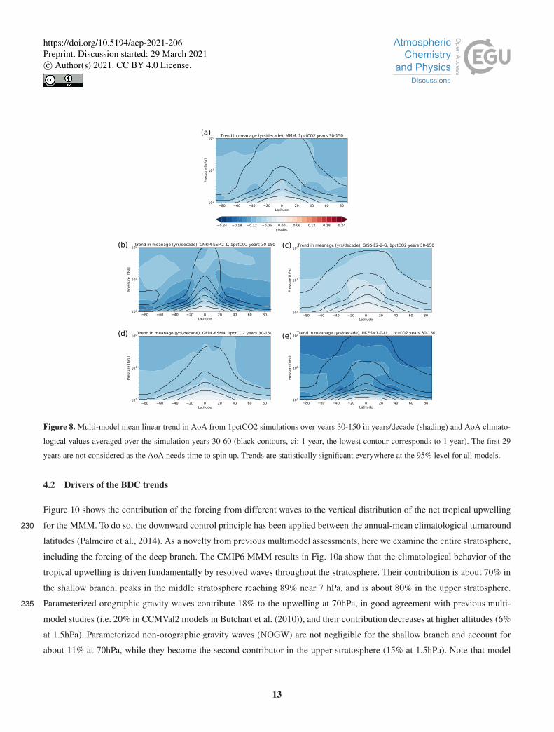
Similar to Fig. 7, Figure 8 shows the AoA trends in the different models and the MMM. The results show a consistent

decrease in mean age throughout the stratosphere. In general there are weaker trends in the lower stratosphere in the SH than

in the NH, consistent with weaker (and even opposite-sign) downwelling trends in this hemisphere seen in Fig. 7. There is210

substantial inter-model spread in the structure and magnitude of the trends. Common features include weaker trends in the

tropical pipe than at high latitudes, and particularly strong trends in the subtropical-midlatitude lower stratosphere.

Figure 9 explores the time dependence of AoA and upwelling trends in the 1pctCO2 runs. This is achieved by plotting trends

for moving 30-year periods for each simulation to find out if trends are approximately constant or if they depend on the period

under consideration. Note that, because there is no comparison with observations, we consider here the same regions for AoA215

and upwelling, representing the shallow and deep branches of the BDC. For individual simulations, the trends vary strongly

for different periods. These variations are the largest for tropical upwelling in the deep branch, with several near-zero and even

negative trend periods (Fig. 9d). These large oscillations in the deep branch upwelling trends are reflected in the MMM, which

shows a quasi-periodicity of about 30 years. In contrast, the upwelling trend in the shallow branch is more consistently positive

throughout the period, and shows an increase in the trend magnitude over time, from 2 to 4 %/decade in the MMM (Fig. 9c).220

The AoA trends are more similar at the two levels, with consistent negative values throughout the period, despite the large

oscillations (Figs. 9a and b).

Figures 5, 6 and 9 demonstrate the high sensitivity of trends in the deep branch residual circulation to the internal variability,

as shown by the large inter-member spread and by the strong dependence on the length and starting year of the trend period.

This contrasts with more stable and less uncertain trends in the shallow branch. They also reveal that AoA is a less noisy225

variable, featuring consistently negative trends in the deep branch across models and members, in contrast to the residual

circulation.

11


Figure 7. Trend in w̄∗ (mm · s−1 · decade−1), computed using 150 year time series from 1pctCO2 experiments. The top left panel shows

multi-model mean (MMM). All other panels show individual models. Turn around latitudes show region of upwelling in first 20 years (solid

red lines) and last 20 years (dashed red lines) of these 150 year simulations. Stippling in top left panel denotes regions where it is not the

case that the trend is significant in at least 66% of models. Stippling in all other panels denotes regions where the trend in that model is not

significant.

12


80 60 40 20 0 20 40 60 80

Latitude

100

101

102

Pre

ssure

[hPa]

Trend in meanage (yrs/decade), UKESM1-0-LL, 1pctCO2 years 30-150

80 60 40 20 0 20 40 60 80

Latitude

100

101

102

Pre

ssure

[hPa]

Trend in meanage (yrs/decade), GISS-E2-2-G, 1pctCO2 years 30-150

80 60 40 20 0 20 40 60 80

Latitude

100

101

102

Pre

ssure

[hPa]

Trend in meanage (yrs/decade), GFDL-ESM4, 1pctCO2 years 30-150

80 60 40 20 0 20 40 60 80

Latitude

100

101

102

Pre

ssure

[hPa]

Trend in meanage (yrs/decade), CNRM-ESM2-1, 1pctCO2 years 30-150

80 60 40 20 0 20 40 60 80

Latitude

100

101

102

Pre

ssure

[hPa]

Trend in meanage (yrs/decade), MMM, 1pctCO2 years 30-150

0.24 0.18 0.12 0.06 0.00 0.06 0.12 0.18 0.24

yrs/dec

(b)

(a)

(c)

(e)(d)

Figure 8. Multi-model mean linear trend in AoA from 1pctCO2 simulations over years 30-150 in years/decade (shading) and AoA climato-

logical values averaged over the simulation years 30-60 (black contours, ci: 1 year, the lowest contour corresponds to 1 year). The first 29

years are not considered as the AoA needs time to spin up. Trends are statistically significant everywhere at the 95% level for all models.

4.2 Drivers of the BDC trends

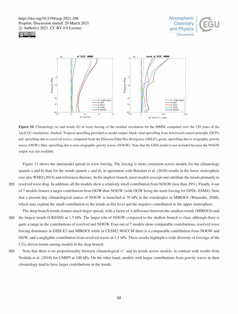
Figure 10 shows the contribution of the forcing from different waves to the vertical distribution of the net tropical upwelling

for the MMM. To do so, the downward control principle has been applied between the annual-mean climatological turnaround230

latitudes (Palmeiro et al., 2014). As a novelty from previous multimodel assessments, here we examine the entire stratosphere,

including the forcing of the deep branch. The CMIP6 MMM results in Fig. 10a show that the climatological behavior of the

tropical upwelling is driven fundamentally by resolved waves throughout the stratosphere. Their contribution is about 70% in

the shallow branch, peaks in the middle stratosphere reaching 89% near 7 hPa, and is about 80% in the upper stratosphere.

Parameterized orographic gravity waves contribute 18% to the upwelling at 70hPa, in good agreement with previous multi-235

model studies (i.e. 20% in CCMVal2 models in Butchart et al. (2010)), and their contribution decreases at higher altitudes (6%

at 1.5hPa). Parameterized non-orographic gravity waves (NOGW) are not negligible for the shallow branch and account for

about 11% at 70hPa, while they become the second contributor in the upper stratosphere (15% at 1.5hPa). Note that model

13


0 20 40 60 80 100 120

Start year

-4

-2

0

2

4

6

8

10

12

w*

trend (

%/d

ecade)

(c) w* trends 70 hPa

0 20 40 60 80 100 120

Start year

-4

-2

0

2

4

6

8

10

12

w*

trend (

%/d

ecade)

(d) w* trends 1.5 hPa

0 20 40 60 80 100 120

Start year

-6

-5

-4

-3

-2

-1

0

1

AoA

tre

nd (

%/d

ecade)

(a) AoA trends 70 hPa

0 20 40 60 80 100 120

Start year

-6

-5

-4

-3

-2

-1

0

1

AoA

tre

nd (

%/d

ecade)

(b) AoA trends 1.5 hPa

CNRM-ESM2-1

CESM2-WACCM

GFDL-ESM4

GISS-E2-2-G

HadGEM3-GC31-LL

MIROC6

MRI-ESM2-0

UKESM1-0-LL

MMM

Figure 9. Trends in AoA (a and b) and upwelling (c and d) at 70 hPa (a and c) and 1.5 hPa (b and d) calculated from 30-years slices of

the 1pctCO2 simulations with start year indicated at x-axis, for each individual simulation (dots, see legend for colors) and the MMM trend

(black). AoA is averaged over 45◦S-45◦N and tropical upwelling is averaged between turnaround latitudes. Note that for upwelling only one

member is included, but for AoA all available members are included (only 9 members for UKESM), in order to have a comparable total

number of simulations for both magnitudes.

output for NOGW drag was available only for a small number of models in previous multi-model assessments, hampering a

direct comparison.240

As noted above, the vertical structure of the trends in upwelling (Fig. 10b) approximately mirrors that of the climatol-

ogy (Fig. 10a). As shown in previous assessments (Butchart et al., 2010; WMO, 2014), resolved waves play the primary role

in driving trends in the shallow branch. This is due to the intensification and upward displacement of the subtropical jets

(not shown) and the upward displacement of the critical lines as discussed in other studies (i.e. Garcia and Randel, 2008;

McLandress and Shepherd, 2009; Shepherd and McLandress, 2011; Hardiman et al., 2014). In particular, at 70hPa, the con-245

tribution to the total trend is 63% resolved waves, 25% OGWs and 11% NOGWs. In the upper stratosphere (above 10 hPa),

resolved waves and NOGW are equally important to the MMM trends, while the contribution from orographic gravity waves

is much smaller. This is in agreement with the results of Palmeiro et al. (2014) for the previous version of WACCM, who ex-

plained the key role of NOGW due to changes in the filtering associated with changes in the background winds with increasing

greenhouse gases. The resolved waves contribution peaks approximately at 7 hPa with a 59% for the MMM. At that level,250

NOGW contribute a 32% and OGW a 9%. At 1.5 hPa the percentages are 48%, 41% and 11%, respectively.

14


-0.5 0 0.5 1.0 1.5

w* (mm/s)

1

5

10

30

50

100

Pre

ssure

(hP

a)

w* DCP, MMM

w*, model output

w* DCP

w* DELF

w* OGW

w* NOGW

-0.01 0 0.02 0.04

w* (mm*s-1 / dec)

1

5

10

30

50

100

Pre

ssure

(hP

a)

trend w* DCP, MMM(a) (b)

w*, model output

w* DCP

w* DELF

w* OGW

w* NOGW

Figure 10. Climatology (a) and trends (b) of wave forcing of the residual circulation for the MMM, computed over the 150 years of the

1pctCO2 simulations. Dashed: Tropical upwelling provided as model output; black: total upwelling from downward control principle (DCP);

red: upwelling due to resolved waves, computed from the Eliassen-Palm flux divergence (DELF); green: upwelling due to orographic gravity

waves (OGW); blue: upwelling due to non-orographic gravity waves (NOGW). Note that the GISS model is not included because the NOGW

output was not available.

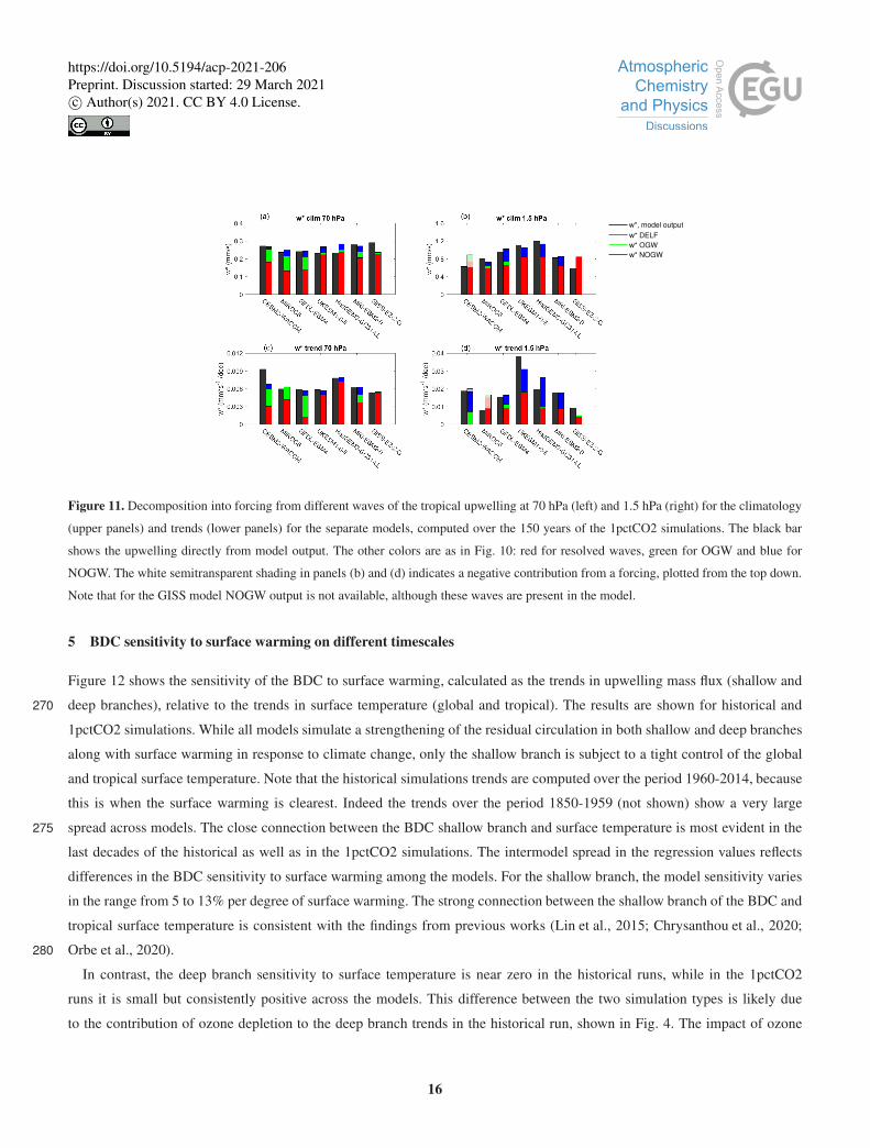
Figure 11 shows the intermodel spread in wave forcing. The forcing is more consistent across models for the climatology

(panels a and b) than for the trends (panels c and d), in agreement with Butchart et al. (2010) results in the lower stratosphere

(see also WMO (2014) and references therein). In the shallow branch, most models (except one) attribute the trends primarily to

resolved wave drag. In addition, all the models show a relatively small contribution from NOGW (less than 20%). Finally, 4 out255

of 7 models feature a larger contribution from OGW than NOGW (with OGW being the main forcing for GFDL-ESM4). Note

that a present-day climatological source of NOGW is launched at 70 hPa in the extratropics in MIROC6 (Watanabe, 2008),

which may explain the small contribution to the trends at this level and the negative contribution in the upper stratosphere.

The deep branch trends feature much larger spread, with a factor of 4 difference between the smallest trends (MIROC6) and

the largest trends (UKESM) at 1.5 hPa. The larger role of NOGW compared to the shallow branch is clear, although there is260

quite a range in the contributions of resolved and NOGW. Four out of 7 models show comparable contributions, resolved wave

forcing dominates in GISS-E2 and MIROC6 while in CESM2-WACCM there is a comparable contribution from NOGW and

OGW, and a negligible contribution from resolved waves at 1.5 hPa. These results highlight a wide diversity of forcings of the

CO2-driven trends among models in the deep branch.

Note that there is no proportionality between climatological w̄∗ and its trends across models, in contrast with results from265

Yoshida et al. (2018) for CMIP5 at 100 hPa. On the other hand, models with larger contributions from gravity waves in their

climatology tend to have larger contributions in the trends.

15


w* DELF

w* OGW

w* NOGW

w*, model output

Figure 11. Decomposition into forcing from different waves of the tropical upwelling at 70 hPa (left) and 1.5 hPa (right) for the climatology

(upper panels) and trends (lower panels) for the separate models, computed over the 150 years of the 1pctCO2 simulations. The black bar

shows the upwelling directly from model output. The other colors are as in Fig. 10: red for resolved waves, green for OGW and blue for

NOGW. The white semitransparent shading in panels (b) and (d) indicates a negative contribution from a forcing, plotted from the top down.

Note that for the GISS model NOGW output is not available, although these waves are present in the model.

5 BDC sensitivity to surface warming on different timescales

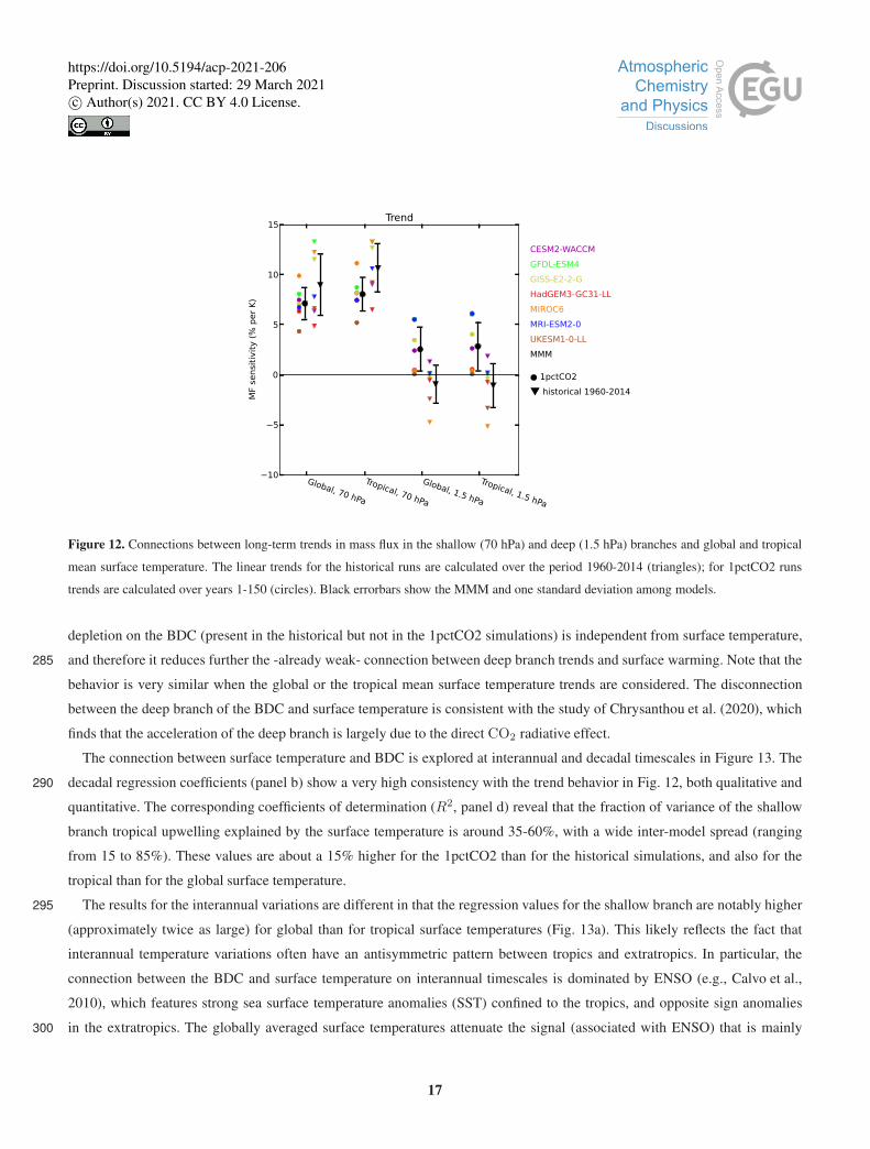
Figure 12 shows the sensitivity of the BDC to surface warming, calculated as the trends in upwelling mass flux (shallow and

deep branches), relative to the trends in surface temperature (global and tropical). The results are shown for historical and270

1pctCO2 simulations. While all models simulate a strengthening of the residual circulation in both shallow and deep branches

along with surface warming in response to climate change, only the shallow branch is subject to a tight control of the global

and tropical surface temperature. Note that the historical simulations trends are computed over the period 1960-2014, because

this is when the surface warming is clearest. Indeed the trends over the period 1850-1959 (not shown) show a very large

spread across models. The close connection between the BDC shallow branch and surface temperature is most evident in the275

last decades of the historical as well as in the 1pctCO2 simulations. The intermodel spread in the regression values reflects

differences in the BDC sensitivity to surface warming among the models. For the shallow branch, the model sensitivity varies

in the range from 5 to 13% per degree of surface warming. The strong connection between the shallow branch of the BDC and

tropical surface temperature is consistent with the findings from previous works (Lin et al., 2015; Chrysanthou et al., 2020;

Orbe et al., 2020).280

In contrast, the deep branch sensitivity to surface temperature is near zero in the historical runs, while in the 1pctCO2

runs it is small but consistently positive across the models. This difference between the two simulation types is likely due

to the contribution of ozone depletion to the deep branch trends in the historical run, shown in Fig. 4. The impact of ozone

16


Global, 70 hPa

Tropical, 70 hPa

Global, 1.5 hPa

Tropical, 1.5 hPa

−10

−5

0

5

10

15

MF sensiti0it1 (% per K)

CESM2-WACCM

GFDL-ESM4

GISS-E2-2-G

HadGEM3-GC31-LL

MIROC6

MRI-ESM2-0

UKESM1-0-LL

MMM

● 1pctCO2▼ historical 1960-2014

Trend

Figure 12. Connections between long-term trends in mass flux in the shallow (70 hPa) and deep (1.5 hPa) branches and global and tropical

mean surface temperature. The linear trends for the historical runs are calculated over the period 1960-2014 (triangles); for 1pctCO2 runs

trends are calculated over years 1-150 (circles). Black errorbars show the MMM and one standard deviation among models.

depletion on the BDC (present in the historical but not in the 1pctCO2 simulations) is independent from surface temperature,

and therefore it reduces further the -already weak- connection between deep branch trends and surface warming. Note that the285

behavior is very similar when the global or the tropical mean surface temperature trends are considered. The disconnection

between the deep branch of the BDC and surface temperature is consistent with the study of Chrysanthou et al. (2020), which

finds that the acceleration of the deep branch is largely due to the direct CO2 radiative effect.

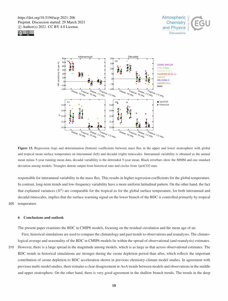
The connection between surface temperature and BDC is explored at interannual and decadal timescales in Figure 13. The

decadal regression coefficients (panel b) show a very high consistency with the trend behavior in Fig. 12, both qualitative and290

quantitative. The corresponding coefficients of determination (R2, panel d) reveal that the fraction of variance of the shallow

branch tropical upwelling explained by the surface temperature is around 35-60%, with a wide inter-model spread (ranging

from 15 to 85%). These values are about a 15% higher for the 1pctCO2 than for the historical simulations, and also for the

tropical than for the global surface temperature.

The results for the interannual variations are different in that the regression values for the shallow branch are notably higher295

(approximately twice as large) for global than for tropical surface temperatures (Fig. 13a). This likely reflects the fact that

interannual temperature variations often have an antisymmetric pattern between tropics and extratropics. In particular, the

connection between the BDC and surface temperature on interannual timescales is dominated by ENSO (e.g., Calvo et al.,

2010), which features strong sea surface temperature anomalies (SST) confined to the tropics, and opposite sign anomalies

in the extratropics. The globally averaged surface temperatures attenuate the signal (associated with ENSO) that is mainly300

17


Global, 70 hPa

Tropical, 70 hPa

Global, 1.5 hPa

Tropical, 1.5 hPa

20

10

0

10

20

30

40

50

60M

F se

nsi

tivit

y (

% p

er

K)

Interannual

(a)

Global, 70 hPa

Tropical, 70 hPa

Global, 1.5 hPa

Tropical, 1.5 hPa

10

5

0

5

10

15

20Decadal

(b)

Global, 70 hPa

Tropical, 70 hPa

Global, 1.5 hPa

Tropical, 1.5 hPa

0.0

0.2

0.4

0.6

0.8

R2

(c)

Global, 70 hPa

Tropical, 70 hPa

Global, 1.5 hPa

Tropical, 1.5 hPa

0.0

0.2

0.4

0.6

0.8

CESM2-WACCM

GFDL-ESM4

GISS-E2-2-G

HadGEM3-GC31-LL

MIROC6

MRI-ESM2-0

UKESM1-0-LL

MMM

1pctCO2 historical

(d)

Figure 13. Regression (top) and determination (bottom) coefficients between mass flux in the upper and lower stratosphere with global

and tropical mean surface temperature on interannual (left) and decadal (right) timescales. Interannual variability is obtained as the annual

mean minus 5-year running mean data, decadal variability is the detrended 5-year mean. Black errorbars show the MMM and one standard

deviation among models. Triangles denote output from historical runs and circles from 1pctCO2 runs.

responsible for interannual variability in the mass flux. This results in higher regression coefficients for the global temperature.

In contrast, long-term trends and low-frequency variability have a more uniform latitudinal pattern. On the other hand, the fact

that explained variances (R2) are comparable for the tropical as for the global surface temperature, for both interannual and

decadal timescales, implies that the surface warming signal on the lower branch of the BDC is controlled primarily by tropical

temperature.305

6 Conclusions and outlook

The present paper examines the BDC in CMIP6 models, focusing on the residual circulation and the mean age of air.

First, historical simulations are used to compare the climatology and past trends to observations and reanalyses. The climato-

logical average and seasonality of the BDC in CMIP6 models lie within the spread of observational (and reanalysis) estimates.

However, there is a large spread in the magnitude among models, which is as large as that across observational estimates. The310

BDC trends in historical simulations are stronger during the ozone depletion period than after, which reflects the important

contribution of ozone depletion to BDC acceleration shown in previous chemistry-climate model studies. In agreement with

previous multi-model studies, there remains a clear disagreement in AoA trends between models and observations in the middle

and upper stratosphere. On the other hand, there is very good agreement in the shallow branch trends. The trends in the deep

18


branch of the residual circulation reveal a large spread among models and across different members of the same model (Figs.315

5, 6). In particular, the inter-member spread in deep branch trends is about ±200% of the ensemble mean trends, even when

considering long (40 year) periods. In contrast, for the shallow branch the spread is 4 times smaller. This reveals a notably

stronger influence of internal variability on the deep branch than the shallow branch trends. In addition, the trends are more

robust for AoA than for upwelling, with inter-member spread in the trends below ±30% for periods slightly longer than 20

years, both in the lower and middle stratosphere.320

The sensitivity of the BDC to CO2 increase is examined, and the robustness of the trends and their wave forcing are explored.

In contrast with previous BDC analyses based on multi-model assessments with CCMI and CCMVal, we focus here on the

response to CO2 alone, using the 1pctCO2 simulations. All models produce stronger BDC acceleration in the NH than in

the SH, and the BDC actually decelerates in the SH polar lower stratosphere, possibly due to the CO2 effects on the polar

vortex discussed in recent works (e.g. Ceppi and Shepherd, 2019). An analysis of the wave forcing of the residual circulation325

shows that shallow branch forcing of climatology and trends is mainly due to resolved waves with a contribution from OGW,

consistent with previous studies. For the deep branch, the main drivers of climatology and trends are resolved waves and

NOGW, but there is a wide spread across models, especially for the trends. There is a very large uncertainty in deep branch

trends (factor of 4 inter-model spread), which could be linked to the spread in forcing. In contrast, the spread in the shallow

branch trends is less than 30%. The uncertainty in deep branch residual circulation trends is emphasized in the large multi-330

decadal fluctuations found over the 150 simulation years. On the other hand, the shallow branch trends are found to increase

over time with CO2 increase, by approximately a factor of 2 for the MMM. In contrast, the AoA trends are more robust over

time, consistent with the results for the historical simulations.

Finally, the connection between surface temperature and the BDC is investigated. We find a strong connection between the

shallow branch and the tropical and global surface temperature. Long-term trends in lower stratospheric upwelling feature a335

sensitivity of 7-10% per degree of surface warming in the models (Fig. 12). On interannual and decadal timescales, surface

temperature explains 35-60% of the shallow branch variance on average (Fig. 13). Note that the strong connection of shallow

branch acceleration with surface warming is consistent with the correlation with the upward shift of the tropopause pointed out

by (Oberländer-Hayn et al., 2016). In contrast, the deep branch variability is not correlated with surface temperature on any

timescale.340

One of the key results of the present paper is the difference between shallow and deep branches of the residual circulation.

The CMIP6 models confirm that, while trends in the shallow branch can now be reconciled with observations (Fu et al., 2015;

WMO, 2018), a clear inconsistency remains for the trends in the deep branch. Our analyses reveal much larger uncertainties in

the deep than in the shallow branch trends, associated with larger internal variability as seen by the inter-member spread. We

note that, while a robust mechanism for the acceleration for the shallow branch has been described (Shepherd and McLandress,345

2011), the drivers of deep branch acceleration remain largely unexplored. Previous studies point to the effects of stratospheric

zonal wind trends on the filtering of NOGW. The CMIP6 model results in the present paper confirm the important role of

NOGW for the deep branch trends. The zonal mean wind trends show acceleration of the polar jet in both hemispheres for the

MMM, but there is a large spread in the trends in the NH, with some models featuring deceleration (not shown). This is con-

19


sistent with large differences in resolved versus NOGW forcing contributions to the deep branch among models. However, the350

compensation mechanism (Cohen et al., 2013; Sigmond and Shepherd, 2014) implies that the different relative contributions

from resolved versus parameterized gravity waves does not necessarily lead to differences in the net BDC trends. Overall, open

questions remain regarding the deep branch trends and their forcing mechanisms. Reducing uncertainties in deep branch trends

is particularly relevant to better constrain the future distribution of ozone in the polar stratosphere, affected not only by direct

transport but also by the descent of ozone-depleting chemical compounds from the mesosphere (Maliniemi et al., 2020).355

The results show that AoA is a much less noisy variable than w̄∗, implying that robust trends could be extracted from rela-

tively short periods (20 years). The advective circulation can be approximated from AoA using the leaky pipe model, in order to

compare with observations, as done in Linz et al. (2016). Unfortunately, the global AoA observational estimates available are

not long enough to evaluate trends. In addition, it is crucial to account for the large uncertainties in deriving AoA trends from

realistic tracers (Fritsch et al., 2020). We note that, for the few models providing both AoA and w̄∗ (3 models for 1pctCO2360

and 4 for historical simulations), it is not possible to extract robust conclusions on the relationship between the strength of

the climatological values or the trends of the two variables. Establishing relations between these two magnitudes would help

evaluate the spread in the magnitude and variability of mixing across models (e.g., Dietmüller et al., 2017; Eichinger et al.,

2018). Based on the results of the present study that highlight the robustness of AoA trends, we suggest that AoA should be a

first-priority consistently defined diagnostic for the next CMIP project (Gerber and Manzini, 2016).365

Data availability. CMIP6 output is available online at various sites listed at https://pcmdi.llnl.gov/CMIP6/.

Author contributions. MA wrote the manuscript with input from all coauthors. MA, NC, SB-B, HG, SCH and PL designed the article and/or

produced figures. MBA, NB, RG, CO, DS-M, SW and KY contributed to the manuscript and provided model expertise.

Competing interests. No competing interests are present.

Acknowledgements. We are thankful to Gabi Stiller for providing the latest version of MIPAS data. MA acknowledges funding from grant370

CGL2017-83198-R (STEADY) and from the Program Atracción de Talento de la Comunidad de Madrid (2016-T2/AMB-1405). HG acknowl-

edges funding from MACClim. PL acknowledges award NA18OAR4320123 from the National Oceanic and Atmospheric Administration,

U.S. Department of Commerce. SW was supported by the Integrated Research Program for Advancing Climate Models (TOUGOU) Grant

Number JPMXD0717935457 and JPMXD0717935715 from the Ministry of Education, Culture, Sports, Science and Technology (MEXT),

Japan. The Earth Simulator at the Japan Agency for Marine-Earth Science and Technology (JAMSTEC) was used for the MIROC6 simula-375

tions.

20


References

Abalos, M., Legras, B., Ploeger, F., and Randel, W. J.: Evaluating the advective Brewer-Dobson circulation in three reanalyses for the period

1979–2012, Journal of Geophysical Research: Atmospheres, 120, 7534–7554, 2015.

Abalos, M., Polvani, L., Calvo, N., Kinnison, D., Ploeger, F., Randel, W., and Solomon, S.: New Insights on the Impact of380

Ozone-Depleting Substances on the Brewer-Dobson Circulation, Journal of Geophysical Research: Atmospheres, 124, 2435–2451,

https://doi.org/10.1029/2018JD029301, http://doi.wiley.com/10.1029/2018JD029301, 2019.

Albers, J. R., Perlwitz, J., Butler, A. H., Birner, T., Kiladis, G. N., Lawrence, Z. D., Manney, G. L., Langford, A. O., and Dias, J.: Mechanisms

Governing Interannual Variability of Stratosphere-to-Troposphere Ozone Transport, Journal of Geophysical Research: Atmospheres, 123,

234–260, https://doi.org/10.1002/2017JD026890, 2018.385

Andrews, A. E., Boering, K. A., Daube, B. C., Wofsy, S. C., Loewenstein, M., Jost, H., Podolske, J. R., Webster, C. R., Herman, R. L., Scott,

D. C., Flesch, G. J., Moyer, E. J., Elkins, J. W., Dutton, G. S., Hurst, D. F., Moore, F. L., Ray, E. A., Romashkin, P. A., and Strahan, S. E.:

Mean ages of stratospheric air derived from in situ observations of CO2, CH4, and N2O, Journal of Geophysical Research Atmospheres,

106, 32 295–32 314, https://doi.org/10.1029/2001JD000465, 2001.

Birner, T.: Residual Circulation and Tropopause Structure, Journal of the Atmospheric Sciences, 67, 2582–2600,390

https://doi.org/10.1175/2010JAS3287.1, http://journals.ametsoc.org/doi/abs/10.1175/2010JAS3287.1, 2010.

Birner, T. and Bönisch, H.: Residual circulation trajectories and transit times into the extratropical lowermost stratosphere, Atmospheric

Chemistry and Physics, 11, 817–827, https://doi.org/10.5194/acp-11-817-2011, 2011.

Butchart, N.: Reviews of Geophysics The Brewer-Dobson circulation, Rev. Geophys, 52, 157–184, https://doi.org/10.1002/2013RG000448,

2014.395

Butchart, N., Cionni, I., Eyring, V., Shepherd, T. G., Waugh, D. W., Akiyoshi, H., Austin, J., Brühl, C., Chipperfield, M. P., Cordero, E.,

Dameris, M., Deckert, R., Dhomse, S., Frith, S. M., Garcia, R. R., Gettelman, A., Giorgetta, M. A., Kinnison, D. E., Li, F., Mancini,

E., Mclandress, C., Pawson, S., Pitari, G., Plummer, D. A., Rozanov, E., Sassi, F., Scinocca, J. F., Shibata, K., Steil, B., and Tian, W.:

Chemistry-climate model simulations of twenty-first century stratospheric climate and circulation changes, Journal of Climate, 23, 5349–

5374, https://doi.org/10.1175/2010JCLI3404.1, 2010.400

Calvo, N., Garcia, R. R., Randel, W. J., and Marsh, D. R.: Dynamical Mechanism for the Increase in Tropical Upwelling

in the Lowermost Tropical Stratosphere during Warm ENSO Events, Journal of the Atmospheric Sciences, 67, 2331–2340,

https://doi.org/10.1175/2010JAS3433.1, 2010.

Ceppi, P. and Shepherd, T. G.: The Role of the Stratospheric Polar Vortex for the Austral Jet Response to Greenhouse Gas Forcing, Geophys-

ical Research Letters, 46, 6972–6979, https://doi.org/10.1029/2019GL082883, 2019.405

Chrysanthou, A., Maycock, A. C., and Chipperfield, M. P.: Decomposing the response of the stratospheric Brewer–Dobson circulation to an

abrupt quadrupling in CO<sub>2</sub>, Weather and Climate Dynamics, 1, 155–174, https://doi.org/10.5194/wcd-1-155-2020, 2020.

Cohen, N. Y., Gerber, E. P., and Bühler, O.: Compensation between Resolved and Unresolved Wave Driving in the Stratosphere: Im-

plications for Downward Control, Journal of the Atmospheric Sciences, 70, 3780–3798, https://doi.org/10.1175/JAS-D-12-0346.1,

http://journals.ametsoc.org/doi/abs/10.1175/JAS-D-12-0346.1, 2013.410

Danabasoglu, G.: NCAR CESM2-WACCM model output prepared for CMIP6 CMIP historical,

https://doi.org/10.22033/ESGF/CMIP6.10071, https://doi.org/10.22033/ESGF/CMIP6.10071, 2019a.

21


Danabasoglu, G.: NCAR CESM2-WACCM model output prepared for CMIP6 CMIP 1pctCO2,

https://doi.org/10.22033/ESGF/CMIP6.10028, https://doi.org/10.22033/ESGF/CMIP6.10028, 2019b.

Dee, D. P., Uppala, S. M., Simmons, A. J., Berrisford, P., Poli, P., Kobayashi, S., Andrae, U., Balmaseda, M. A., Balsamo, G., Bauer,415

P., Bechtold, P., Beljaars, A. C. M., van de Berg, L., Bidlot, J., Bormann, N., Delsol, C., Dragani, R., Fuentes, M., Geer, A. J., Haim-

berger, L., Healy, S. B., Hersbach, H., H??lm, E. V., Isaksen, L., K??llberg, P., K??hler, M., Matricardi, M., Mcnally, A. P., Monge-Sanz,

B. M., Morcrette, J. J., Park, B. K., Peubey, C., de Rosnay, P., Tavolato, C., Th??paut, J. N., and Vitart, F.: The ERA-Interim reanalysis:

Configuration and performance of the data assimilation system, Quarterly Journal of the Royal Meteorological Society, 137, 553–597,

https://doi.org/10.1002/qj.828, 2011.420

Dietmüller, S., Garny, H., Plöger, F., Jöckel, P., and Cai, D.: Effects of mixing on resolved and unresolved scales on stratospheric age of air,

Atmospheric Chemistry and Physics, 17, 7703–7719, https://doi.org/10.5194/acp-17-7703-2017, 2017.

Dunne, J. P., Horowitz, L. W., Adcroft, A. J., Ginoux, P., Held, I. M., John, J. G., Krasting, J. P., Malyshev, S., Naik, V., Paulot, F., Shevli-

akova, E., Stock, C. A., Zadeh, N., Balaji, V., Blanton, C., Dunne, K. A., Dupuis, C., Durachta, J., Dussin, R., Gauthier, P. P., Griffies,

S. M., Guo, H., Hallberg, R. W., Harrison, M., He, J., Hurlin, W., McHugh, C., Menzel, R., Milly, P. C., Nikonov, S., Paynter, D. J.,425

Ploshay, J., Radhakrishnan, A., Rand, K., Reichl, B. G., Robinson, T., Schwarzkopf, D. M., Sentman, L. T., Underwood, S., Vahlenkamp,

H., Winton, M., Wittenberg, A. T., Wyman, B., Zeng, Y., and Zhao, M.: The GFDL Earth System Model Version 4.1 (GFDL-ESM

4.1): Overall Coupled Model Description and Simulation Characteristics, Journal of Advances in Modeling Earth Systems, 12, 1–56,

https://doi.org/10.1029/2019MS002015, 2020.

Eichinger, R., Dietmüller, S., Garny, H., Sacha, P., Birner, T., Böhnisch, H., Pitari, G., Visioni, D., Stenke, A., Rozanov, E., Revell, L.,430

Plummer, D. A., Jöckel, P., Oman, L., Deushi, M., Kinnison, D. E., Garcia, R., Morgenstern, O., Zeng, G., Stone, K. A., and Schofield,

R.: The influence of mixing on stratospheric circulation changes in the 21st century, Atmospheric Chemistry and Physics Discussions, pp.

1–31, https://doi.org/10.5194/acp-2018-1110, 2018.

Emanuel, K., Solomon, S., Folini, D., Davis, S., and Cagnazzo, C.: Influence of tropical tropopause layer cooling on atlantic hurricane

activity, Journal of Climate, 26, 2288–2301, https://doi.org/10.1175/JCLI-D-12-00242.1, 2013.435

Engel, A., Bönisch, H., Ullrich, M., Sitals, R., Membrive, O., Danis, F., and Crevoisier, C.: Mean age of stratospheric air derived from

AirCore observations, Atmospheric Chemistry and Physics, 17, 6825–6838, https://doi.org/10.5194/acp-17-6825-2017, 2017.

Eyring, V., Bony, S., Meehl, G. A., Senior, C. A., Stevens, B., Stouffer, R. J., and Taylor, K. E.: Overview of the Coupled Model

Intercomparison Project Phase 6 (CMIP6) experimental design and organization, Geoscientific Model Development, 9, 1937–1958,

https://doi.org/10.5194/gmd-9-1937-2016, 2016.440

Fritsch, F., Garny, H., Engel, A., Bönisch, H., and Eichinger, R.: Sensitivity of age of air trends to the derivation

method for non-linear increasing inert SF 6, Atmos. Chem. Phys, 20, 8709–8725, https://doi.org/10.5194/acp-20-8709-2020,

https://doi.org/10.5194/acp-20-8709-2020, 2020.

Fu, Q., Lin, P., Solomon, S., and Hartmann, D. L.: Observational evidence of strengthening of the Brewer-Dobson circulation since 1980,

Journal of Geophysical Research : Atmospheres, 120, 10,214–10,228, https://doi.org/10.1002/2015JD023657, 2015.445

Garcia, R. R. and Randel, W. J.: Acceleration of the Brewer–Dobson Circulation due to Increases in Greenhouse Gases, Journal of the

Atmospheric Sciences, 65, 2731–2739, https://doi.org/10.1175/2008JAS2712.1, 2008.

Garcia, R. R., Dunkerton, T. J., Lieberman, R. S., and Vincent, R. A.: Climatology of the semiannual oscillation of the tropical middle

atmosphere, Journal of Geophysical Research Atmospheres, 102, 19–26, https://doi.org/10.1029/97jd00207, 1997.

22


Garny, H., Birner, T., Bönisch, H., and Bunzel, F.: The effects of mixing on age of air, Journal of Geophysical Research: Atmospheres, 119,450

7015–7034, https://doi.org/10.1002/2013JD021417, http://doi.wiley.com/10.1002/2013JD021417, 2014.

Gerber, E. P. and Manzini, E.: The Dynamics and Variability Model Intercomparison Project (DynVarMIP) for CMIP6: Assessing the

stratosphere-troposphere system, Geoscientific Model Development, 9, 3413–3425, https://doi.org/10.5194/gmd-9-3413-2016, 2016.

Gettelman, A., Mills, M. J., Kinnison, D. E., Garcia, R. R., Smith, A. K., Marsh, D. R., Tilmes, S., Vitt, F., Bardeen, C. G., McInerny, J., Liu,

H.-L., Solomon, S. C., Polvani, L. M., Emmons, L. K., Lamarque, J.-F., Richter, J. H., Glanville, A. S., Bacmeister, J. T., Phillips, A. S.,455

Neale, R. B., Simpson, I. R., DuVivier, A. K., Hodzic, A., and Randel, W. J.: The Whole Atmosphere Community Climate Model Version 6

(WACCM6), Journal of Geophysical Research: Atmospheres, 124, 12 380–12 403, https://doi.org/https://doi.org/10.1029/2019JD030943,

https://agupubs.onlinelibrary.wiley.com/doi/abs/10.1029/2019JD030943, 2019.

Haenel, F. J., Stiller, G. P., Von Clarmann, T., Funke, B., Eckert, E., Glatthor, N., Grabowski, U., Kellmann, S., Kiefer, M., Linden, A.,

and Reddmann, T.: Reassessment of MIPAS age of air trends and variability, Atmospheric Chemistry and Physics, 15, 13 161–13 176,460

https://doi.org/10.5194/acp-15-13161-2015, 2015.

Hardiman, S. C., Butchart, N., and Calvo, N.: The morphology of the Brewer-Dobson circulation and its response to climate change in

CMIP5 simulations, Quarterly Journal of the Royal Meteorological Society, 140, 1958–1965, https://doi.org/10.1002/qj.2258, 2014.

Hardiman, S. C., Lin, P., Scaife, A. A., Dunstone, N. J., and Ren, H. L.: The influence of dynamical variability on the observed Brewer-

Dobson circulation trend, Geophysical Research Letters, 44, 2885–2892, https://doi.org/10.1002/2017GL072706, 2017.465

Kim, J., Randel, W., Birner, T., and Abalos, M.: Spectrum of wave forcing associated with the annual cycle of upwelling at the tropical

tropopause, Journal of the Atmospheric Sciences, 73, https://doi.org/10.1175/JAS-D-15-0096.1, 2016.

Kobayashi, S., Ota, Y., Harada, Y., Ebita, A., Moriya, M., Onoda, H., Onogui, K., Kamahori, H., Kobayashi, C., Endo, H., Miyaoka, K., and

Takahashi, K.: The JRA-55 Reanalysis: General Specifications and Basic Characteristics, Journal of the Meteorological Society of Japan.

Ser. II, 93, 5–48, https://doi.org/10.2151/jmsj.2015-001, https://www.jstage.jst.go.jp/article/jmsj/93/1/93{_}2015-001/{_}article, 2015.470

Krasting, J. P., John, J. G., Blanton, C., McHugh, C., Nikonov, S., Radhakrishnan, A., Rand, K., Zadeh, N. T., Balaji, V., Durachta, J., Dupuis,

C., Menzel, R., Robinson, T., Underwood, S., Vahlenkamp, H., Dunne, K. A., Gauthier, P. P., Ginoux, P., Griffies, S. M., Hallberg, R.,

Harrison, M., Hurlin, W., Malyshev, S., Naik, V., Paulot, F., Paynter, D. J., Ploshay, J., Schwarzkopf, D. M., Seman, C. J., Silvers, L.,

Wyman, B., Zeng, Y., Adcroft, A., Dunne, J. P., Dussin, R., Guo, H., He, J., Held, I. M., Horowitz, L. W., Lin, P., Milly, P., Shevliakova,

E., Stock, C., Winton, M., Xie, Y., and Zhao, M.: NOAA-GFDL GFDL-ESM4 model output prepared for CMIP6 CMIP historical,475


Krasting, J. P., John, J. G., Blanton, C., McHugh, C., Nikonov, S., Radhakrishnan, A., Rand, K., Zadeh, N. T., Balaji, V., Durachta, J.,

Dupuis, C., Menzel, R., Robinson, T., Underwood, S., Vahlenkamp, H., Dunne, K. A., Gauthier, P. P., Ginoux, P., Griffies, S. M., Hallberg,

R., Harrison, M., Hurlin, W., Malyshev, S., Naik, V., Paulot, F., Paynter, D. J., Ploshay, J., Schwarzkopf, D. M., Seman, C. J., Silvers,

L., Wyman, B., Zeng, Y., Adcroft, A., Dunne, J. P., Dussin, R., Guo, H., He, J., Held, I. M., Horowitz, L. W., Lin, P., Milly, P., Shevli-480

akova, E., Stock, C., Winton, M., Xie, Y., and Zhao, M.: NOAA-GFDL GFDL-ESM4 model output prepared for CMIP6 CMIP 1pctCO2,


Li, F., Newman, P., Pawson, S., and Perlwitz, J.: Effects of Greenhouse Gas Increase and Stratospheric Ozone Depletion on Strato-

spheric Mean Age of Air in 1960-2010, Journal of Geophysical Research: Atmospheres, pp. 1–13, https://doi.org/10.1002/2017JD027562,

http://doi.wiley.com/10.1002/2017JD027562, 2018.485

Lin, P., Ming, Y., and Ramaswamy, V.: Tropical climate change control of the lower stratospheric circulation, Geophysical Research Letters,

42, 941–948, https://doi.org/10.1002/2014GL062823, 2015.

23


Linz, M., Plumb, R. A., Gerber, E. P., and Sheshadri, A.: The Relationship between Age of Air and the Diabatic Cir-

culation of the Stratosphere, Journal of the Atmospheric Sciences, 73, 4507–4518, https://doi.org/10.1175/JAS-D-16-0125.1,

http://journals.ametsoc.org/doi/10.1175/JAS-D-16-0125.1, 2016.490

Maliniemi, V., Marsh, Daniel, R., Tyssøy, H. N., and Smith-Johnsen, C.: Will Climate Change Impact Polar NOx Produced by Energetic

Particle Precipitation?, Geophysical Research Letters, 47, 1–10, https://doi.org/10.1029/2020GL087041, 2020.

Manzini, E., Karpechko, A. Y., Anstey, J., Baldwin, M. P., Black, R. X., Cagnazzo, C., Calvo, N., Charlton-Perez, A., Christiansen,

B., Davini, P., Gerber, E., Giorgetta, M., Gray, L., Hardiman, S. C., Lee, Y.-Y., Marsh, D. R., McDaniel, B. A., Purich, A.,

Scaife, A. A., Shindell, D., Son, S.-W., Watanabe, S., and Zappa, G.: Northern winter climate change: Assessment of uncertainty495

in CMIP5 projections related to stratosphere-troposphere coupling, Journal of Geophysical Research: Atmospheres, 119, 7979–7998,

https://doi.org/10.1002/2013JD021403, http://doi.wiley.com/10.1002/2013JD021403, 2014.

McLandress, C. and Shepherd, T. G.: Simulated anthropogenic changes in the Brewer-Dobson circulation, including its extension to high

latitudes, Journal of Climate, 22, 1516–1540, https://doi.org/10.1175/2008JCLI2679.1, 2009.

McLandress, C., Jonsson, A. I., Plummer, D. A., Reader, M. C., Scinocca, J. F., and Shepherd, T. G.: Separating the dynami-500

cal effects of climate change and ozone depletion. Part I: Southern hemisphere stratosphere, Journal of Climate, 23, 5002–5020,

https://doi.org/10.1175/2010JCLI3586.1, 2010.

NASA/GISS, N. G. I. f. S. S.: NASA-GISS GISS-E2-2-G model output prepared for CMIP6 CMIP,

https://doi.org/10.22033/ESGF/CMIP6.2081, https://doi.org/10.22033/ESGF/CMIP6.2081, 2019.

Oberländer-Hayn, S., Gerber, E. P., Abalichin, J., Akiyoshi, H., Kerschbaumer, A., Kubin, A., Kunze, M., Langematz, U., Meul, S., Michou,505

M., Morgenstern, O., and Oman, L. D.: Is the Brewer-Dobson circulation increasing or moving upward?, Geophysical Research Letters,

43, 1772–1779, https://doi.org/10.1002/2015GL067545, 2016.

Oman, L., Waugh, D. W., Pawson, S., Stolarski, R. S., and Newman, P. A.: On the influence of anthropogenic forcings on changes in the

stratospheric mean age, Journal of Geophysical Research Atmospheres, 114, 1–15, https://doi.org/10.1029/2008JD010378, 2009.

Orbe, C., Rind, D., Jonas, J., Nazarenko, L., Faluvegi, G., Murray, L. T., Shindell, D. T., Tsigaridis, K., Zhou, T., Kelley, M., and Schmidt,510

G. A.: GISS Model E2.2: A Climate Model Optimized for the Middle Atmosphere—2. Validation of Large-Scale Transport and Evaluation

of Climate Response, Journal of Geophysical Research: Atmospheres, 125, https://doi.org/10.1029/2020JD033151, 2020.

Ortland, D. A. and Alexander, M. J.: The residual-mean circulation in the tropical tropopause layer driven by tropical waves, Journal of the

Atmospheric Sciences, 71, 1305–1322, https://doi.org/10.1175/JAS-D-13-0100.1, 2014.

Palmeiro, F. M., Calvo, N., and Garcia, R. R.: Future Changes in the Brewer–Dobson Circulation under Different Greenhouse515

Gas Concentrations in WACCM4, Journal of the Atmospheric Sciences, 71, 2962–2975, https://doi.org/10.1175/JAS-D-13-0289.1,

http://journals.ametsoc.org/doi/abs/10.1175/JAS-D-13-0289.1, 2014.

Ploeger, F., Abalos, M., Birner, T., Konopka, P., Legras, B., Müller, R., and Riese, M.: Quantifying the effects of mixing and residual

circulation on trends of stratospheric mean age of air, Geophysical Research Letters, 42, https://doi.org/10.1002/2014GL062927, 2015.

Plumb, R. A.: Stratospheric Transport., Journal of the Meteorological Society of Japan, 80, 793–809, https://doi.org/10.2151/jmsj.80.793,520

http://joi.jlc.jst.go.jp/JST.JSTAGE/jmsj/80.793?from=CrossRef, 2002.

Polvani, L. M., Abalos, M., Garcia, R., Kinnison, D., and Randel, W. J.: Significant Weakening of Brewer-Dobson Circula-

tion Trends Over the 21st Century as a Consequence of the Montreal Protocol, Geophysical Research Letters, 45, 401–409,

https://doi.org/10.1002/2017GL075345, http://doi.wiley.com/10.1002/2017GL075345, 2018.

24


Polvani, L. M., Wang, L., Abalos, M., Butchart, N., Chipperfield, M. P., Dameris, M., Deushi, M., Dhomse, S. S., Jöckel, P., Kinnison,525

D., Michou, M., Morgenstern, O., Oman, L. D., Plummer, D. A., and Stone, K. A.: Large Impacts, Past and Future, of Ozone-Depleting

Substances on Brewer-Dobson Circulation Trends: A Multimodel Assessment, Journal of Geophysical Research: Atmospheres, 124,

6669–6680, https://doi.org/10.1029/2018JD029516, 2019.

Randel, W. and Park, M.: Diagnosing Observed Stratospheric Water Vapor Relationships to the Cold Point Tropical Tropopause, Journal of

Geophysical Research: Atmospheres, 124, 7018–7033, https://doi.org/10.1029/2019JD030648, 2019.530

Randel, W. J., Garcia, R. R., and Wu, F.: Dynamical balances and tropical stratospheric upwelling, Journal of the Atmospheric Sciences, 65,

3584–3595, https://doi.org/10.1175/2008JAS2756.1, 2008.

Ridley, J., Menary, M., Kuhlbrodt, T., Andrews, M., and Andrews, T.: MOHC HadGEM3-GC31-LL model output prepared for CMIP6 CMIP

historical, https://doi.org/10.22033/ESGF/CMIP6.6109, https://doi.org/10.22033/ESGF/CMIP6.6109, 2019a.

Ridley, J., Menary, M., Kuhlbrodt, T., Andrews, M., and Andrews, T.: MOHC HadGEM3-GC31-LL model output prepared for CMIP6 CMIP535

1pctCO2, https://doi.org/10.22033/ESGF/CMIP6.5788, 2019b.

Rienecker, M. M., Suarez, M. J., Gelaro, R., Todling, R., Bacmeister, J., Liu, E., Bosilovich, M. G., Schubert, S. D., Takacs, L., Kim, G. K.,

Bloom, S., Chen, J., Collins, D., Conaty, A., Da Silva, A., Gu, W., Joiner, J., Koster, R. D., Lucchesi, R., Molod, A., Owens, T., Pawson,

S., Pegion, P., Redder, C. R., Reichle, R., Robertson, F. R., Ruddick, A. G., Sienkiewicz, M., and Woollen, J.: MERRA: NASA’s modern-

era retrospective analysis for research and applications, Journal of Climate, 24, 3624–3648, https://doi.org/10.1175/JCLI-D-11-00015.1,540

2011.

Rind, D., Orbe, C., Jonas, J., Nazarenko, L., Zhou, T., Kelley, M., Lacis, A., Shindell, D., Faluvegi, G., Russell, G., Bauer, M., Schmidt, G.,

Romanou, A., and Tausnev, N.: GISS Model E2.2: A climate model optimized for the middle atmosphere — Model structure, climatology,

variability and climate sensitivity, J. Geophys. Res. Atmos., 125, e2019JD032 204, https://doi.org/10.1029/2019JD032204, 2020.

Rosenlof, K. H.: Seasonal cycle of the residual mean meridional circulation in the stratosphere, Journal of Geophysical Research, 100,545

5173–5191, https://doi.org/10.1029/94JD03122, 1995.

Seferian, R.: CNRM-CERFACS CNRM-ESM2-1 model output prepared for CMIP6 CMIP historical,


Seferian, R.: CNRM-CERFACS CNRM-ESM2-1 model output prepared for CMIP6 CMIP for experiment 1pctCO2,

https://doi.org/10.22033/ESGF/CMIP6.3714, https://doi.org/10.22033/ESGF/CMIP6.3714, 2018b.550

Sellar, A. A., Jones, C. G., Mulcahy, J. P., Tang, Y., Yool, A., Wiltshire, A., O’Connor, F. M., Stringer, M., Hill, R., Palmieri, J., Woodward,

S., de Mora, L., Kuhlbrodt, T., Rumbold, S. T., Kelley, D. I., Ellis, R., Johnson, C. E., Walton, J., Abraham, N. L., Andrews, M. B.,

Andrews, T., Archibald, A. T., Berthou, S., Burke, E., Blockley, E., Carslaw, K., Dalvi, M., Edwards, J., Folberth, G. A., Gedney, N.,

Griffiths, P. T., Harper, A. B., Hendry, M. A., Hewitt, A. J., Johnson, B., Jones, A., Jones, C. D., Keeble, J., Liddicoat, S., Morgenstern,

O., Parker, R. J., Predoi, V., Robertson, E., Siahaan, A., Smith, R. S., Swaminathan, R., Woodhouse, M. T., Zeng, G., and Zerroukat, M.:555

UKESM1: Description and Evaluation of the U.K. Earth System Model, Journal of Advances in Modeling Earth Systems, 11, 4513–4558,

https://doi.org/https://doi.org/10.1029/2019MS001739, https://agupubs.onlinelibrary.wiley.com/doi/abs/10.1029/2019MS001739, 2019.

Shepherd, T. G. and McLandress, C.: A robust mechanism for strengthening of the Brewer–Dobson circulation in response

to climate change: critical-layer control of subtropical wave breaking, Journal of the Atmospheric Sciences, 68, 784–797,

https://doi.org/10.1175/2010JAS3608.1, 2011.560

25


Sigmond, M. and Shepherd, T. G.: Compensation between resolved wave driving and parameterized orographic gravity

wave driving of the Brewer-Dobson circulation and its response to climate change, Journal of Climate, 27, 5601–5610,

https://doi.org/10.1175/JCLI-D-13-00644.1, 2014.

Stiller, G. P., Von Clarmann, T., Haenel, F., Funke, B., Glatthor, N., Grabowski, U., Kellmann, S., Kiefer, M., Linden, A., Lossow, S.,

and López-Puertas, M.: Observed temporal evolution of global mean age of stratospheric air for the 2002 to 2010 period, Atmospheric565

Chemistry and Physics, 12, 3311–3331, https://doi.org/10.5194/acp-12-3311-2012, 2012.

Stiller, G. P., Harrison, J. J., Haenel, F. J., Glatthor, N., Kellmann, S., and von Clarmann, T.: Improved global distributions of SF6

and mean age of stratospheric air by use of new spectroscopic data, in: EGU2020-2660, edited by EGU General Assembly 2020,

https://doi.org/https://doi.org/10.5194/egusphere-egu2020-2660, https://doi.org/10.5194/egusphere-egu2020-2660, 2020.

Séférian, R., Nabat, P., Michou, M., Saint-Martin, D., Voldoire, A., Colin, J., Decharme, B., Delire, C., Berthet, S., Chevallier, M., Sénési,570

S., Franchisteguy, L., Vial, J., Mallet, M., Joetzjer, E., Geoffroy, O., Guérémy, J.-F., Moine, M.-P., Msadek, R., Ribes, A., Rocher,

M., Roehrig, R., Salas-y Mélia, D., Sanchez, E., Terray, L., Valcke, S., Waldman, R., Aumont, O., Bopp, L., Deshayes, J., Éthé, C.,

and Madec, G.: Evaluation of CNRM Earth System Model, CNRM-ESM2-1: Role of Earth System Processes in Present-Day and Fu-

ture Climate, Journal of Advances in Modeling Earth Systems, 11, 4182–4227, https://doi.org/https://doi.org/10.1029/2019MS001791,

https://agupubs.onlinelibrary.wiley.com/doi/abs/10.1029/2019MS001791, 2019.575

Tang, Y., Rumbold, S., Ellis, R., Kelley, D., Mulcahy, J., Sellar, A., Walton, J., and Jones, C.: MOHC UKESM1.0-LL model output prepared

for CMIP6 CMIP historical, https://doi.org/10.22033/ESGF/CMIP6.6113, https://doi.org/10.22033/ESGF/CMIP6.6113, 2019a.

Tang, Y., Rumbold, S., Ellis, R., Kelley, D., Mulcahy, J., Sellar, A., Walton, J., and Jones, C.: MOHC UKESM1.0-LL model output prepared

for CMIP6 CMIP 1pctCO2, https://doi.org/10.22033/ESGF/CMIP6.5792, https://doi.org/10.22033/ESGF/CMIP6.5792, 2019b.

Tatebe, H. and Watanabe, M.: MIROC MIROC6 model output prepared for CMIP6 CMIP historical,580


Tatebe, H. and Watanabe, M.: MIROC MIROC6 model output prepared for CMIP6 CMIP 1pctCO2,


Tatebe, H., Ogura, T., Nitta, T., Komuro, Y., Ogochi, K., Takemura, T., Sudo, K., Sekiguchi, M., Abe, M., Saito, F., Chikira, M., Watanabe, S.,

Mori, M., Hirota, N., Kawatani, Y., Mochizuki, T., Yoshimura, K., Takata, K., O’ishi, R., Yamazaki, D., Suzuki, T., Kurogi, M., Kataoka,585

T., Watanabe, M., , and Kimoto, M.: Description and basic evaluation of simulated mean state, internal variability, and climate sensitivity

in MIROC6, Geoscientific Model Development, 12, 2727–2765, https://doi.org/https://doi.org/10.5194/gmd-12-2727-2019, 2019.

Ueyama, R., Gerber, E. P., Wallace, J. M., and Frierson, D. M. W.: The Role of High-Latitude Waves in the Intraseasonal to Sea-

sonal Variability of Tropical Upwelling in the Brewer–Dobson Circulation, Journal of the Atmospheric Sciences, 70, 1631–1648,

https://doi.org/10.1175/JAS-D-12-0174.1, http://journals.ametsoc.org/doi/abs/10.1175/JAS-D-12-0174.1, 2013.590

Watanabe, S.: Constraints on a non-orographic gravity wave drag parameterization using a gravity wave resolving general circulation model,

Scientific Online Letters on the Atmosphere, 4, 61–64, https://doi.org/10.2151/sola.2008-016, 2008.

Williams, K. D., Copsey, D., Blockley, E. W., Bodas-Salcedo, A., Calvert, D., Comer, R., Davis, P., Graham, T., Hewitt, H. T., Hill, R., Hyder,

P., Ineson, S., Johns, T. C., Keen, A. B., Lee, R. W., Megann, A., Milton, S. F., Rae, J. G. L., Roberts, M. J., Scaife, A. A., Schiemann,

R., Storkey, D., Thorpe, L., Watterson, I. G., Walters, D. N., West, A., Wood, R. A., Woollings, T., and Xavier, P. K.: The Met Office595

Global Coupled Model 3.0 and 3.1 (GC3.0 and GC3.1) Configurations, Journal of Advances in Modeling Earth Systems, 10, 357–380,

https://doi.org/https://doi.org/10.1002/2017MS001115, https://agupubs.onlinelibrary.wiley.com/doi/abs/10.1002/2017MS001115, 2018.

26


WMO: WMO (World Meteorological Organization), Scientific Assessment of Ozone Depletion: 2014 Global Ozone Research and Monitor-

ing Project-Report, World Meteorological Organization, Geneva, Switzerland, 2014.

WMO: Scientific Assessment of Ozone Depletion: 2018, World Meteorological Organisation Global Ozone Research and Monitoring600

Project-Report No. 58, 58, http://ozone.unep.org/science/assessment/sap, 2018.

Yoshida, K., Mizuta, R., and Arakawa, O.: Intermodel Differences in Upwelling in the Tropical Tropopause Layer Among CMIP5 Models,

Journal of Geophysical Research: Atmospheres, 123, 13,658–13,675, https://doi.org/10.1029/2018JD029044, 2018.

Young, P. J., Thompson, D. W., Rosenlof, K. H., Solomon, S., and Lamarque, J. F.: The seasonal cycle and interannual variability in strato-

spheric temperatures and links to the Brewer-Dobson circulation: An analysis of MSU and SSU data, Journal of Climate, 24, 6243–6258,605

https://doi.org/10.1175/JCLI-D-10-05028.1, 2011.

Yukimoto, S., Kawai, H., Koshiro, T., Oshima, N., Yoshida, K., Urakawa, S., Tsujino, H., Deushi, M., Tanaka, T., Hosaka, M., Yabu, S.,

Yoshimura, H., Shindo, E., Mizuta, R., Obata, A., Adachi, Y., and Ishii, M.: The Meteorological Research Institute Earth System Model

Version 2.0, MRI-ESM2.0: Description and Basic Evaluation of the Physical Component, Journal of the Meteorological Society of Japan.

Ser. II, 97, 931–965, https://doi.org/10.2151/jmsj.2019-051, 2019a.610

Yukimoto, S., Koshiro, T., Kawai, H., Oshima, N., Yoshida, K., Urakawa, S., Tsujino, H., Deushi, M., Tanaka, T., Hosaka, M., Yoshimura,

H., Shindo, E., Mizuta, R., Ishii, M., Obata, A., and Adachi, Y.: MRI MRI-ESM2.0 model output prepared for CMIP6 CMIP historical,


Yukimoto, S., Koshiro, T., Kawai, H., Oshima, N., Yoshida, K., Urakawa, S., Tsujino, H., Deushi, M., Tanaka, T., Hosaka, M., Yoshimura,

H., Shindo, E., Mizuta, R., Ishii, M., Obata, A., and Adachi, Y.: MRI MRI-ESM2.0 model output prepared for CMIP6 CMIP 1pctCO2,615

https://doi.org/10.22033/ESGF/CMIP6.5356, https://doi.org/10.22033/ESGF/CMIP6.5356, 2019c.

27


Documents

The Brewer-Dobsoncirculation in CMIP6