The Causal Effect of Trade on Migration:

Evidence from Countries of the

Euro-Mediterranean Partnership

Nadia Campaniello∗

March 28, 2014

Abstract

In the attempt to reduce migration pressure, since 1995, the EuropeanUnion has been planning to establish a free trade area with developing coun-tries bordering the Mediterranean Sea. The process is still ongoing. Ourpaper tests whether it is likely to be an effective policy. We estimate a gravi-tational model of bilateral migrations on bilateral exports from the Mediter-ranean Third Countries (South) to the European Union (North) over theperiod 1970-2000, using different specifications. We find, in line with most ofthe literature, a significantly positive correlation (called “complementarity”)between exports and migrations from the South to the North. Then we go onestep further, trying to solve the potential endogeneity problem using averagetrade tariffs and bilateral exchange rate volatility as instruments for trade.Based on the OLS as well as the 2SLS results, liberalizing trade in the area ofthe Euro-Mediterranean partnership does not seem to be an effective policyto mitigate the migration flows, at least in the short run.

Keywords: International trade, Migration, Causality, Gravity Model, Euro-Mediterranean partnership, Exchange Rate VolatilityJEL classification codes: F15, F16, F22

Acknowledgements: A special thank to Francesc Ortega, Giovanni Mastrobuoni,Tommaso Frattini, Greg Wright, Tim Hatton, Abhishek Chakravarty, Stefano Bo-latto, Gianluigi Vernasca, Joshua R. Goldstein and Guy Stecklov for their usefulsuggestions. Finally we thank all the participants to the 2013 Alpine PopulationConference, to the 25th Annual Conference of the European Association of LabourEconomists and to the Essex FRESH Meeting for their useful comments.

∗University of Essex, UK, ncampa@essex.ac.uk

1 Introduction

The relationship between international trade and migration has been long debated,

especially for its policy implications.

The use of trade policy to deal with the migration problem has been consid-

ered by both the European Union and the United States policy-makers. Their view

is that opening their markets to exports from countries in the South reduces the

pressure to migrate. In particular, Presidents Carlos Salinas and George H. W.

Bush argued that the North American Free Trade Agreement (NAFTA) would have

helped Mexico to export more goods and less people, while EU countries hope, more

or less explicitly, that migration flows from the South Mediterranean shore to the

North will decrease as a consequence of the beneficial impact of trade liberalisation

on employment and living standards in the sending countries (Garson, 1998). These

statements are based on the view that trade liberalization would have increased the

level of exports from the Southern countries increasing labour demand and wages in

the same countries, therefore decreasing migration from these countries.

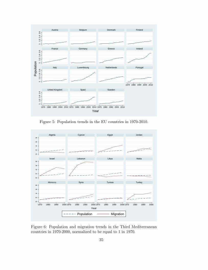
Zimmermann (1995) suggests that stagnating and aging populations like those of

the European Union tend to attract migrants, while young and large populations,

like those of North Africa, tend to be more prone to move. In Figure 5 (in the

appendix) we plot the population trends in each of the European country that we

consider in our analysis. The population growth has been very low, on average 14%,

between 1970 and 2010. Since we use official data on migration and do not have

information on the illegal migrants, such numbers represent lower bounds. All the

Third Mediterranean Countries (TMCs) show larger increasing trends in population

6 (in the appendix). With a few exceptions, migration flows are also trending up-

2

wards. 1

This evidence suggests that migrations to Europe will keep on being a major concern

in the next few decades. For this reason the EU has shown an increasing interest

in the Mediterranean region and has tried to create an interregional framework of

cooperation that could contribute to prevent the Mediterranean to be a conflicting

frontier. In 1995 the European Union signed the Barcelona Declaration that is the

founding act of a partnership between the European Union and twelve countries

in the Southern Mediterranean (now re-launched with the Union for the Mediter-

ranean) to help the economic development of the Third Mediterranean Countries,

especially through trade liberalization, in an attempt to reduce migratory flows

from such areas. This paper is going to test whether this policy is likely to be

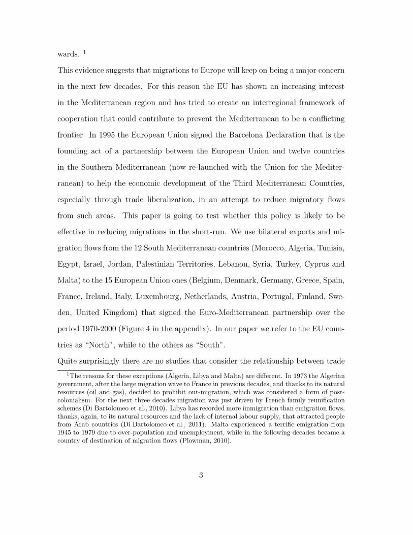
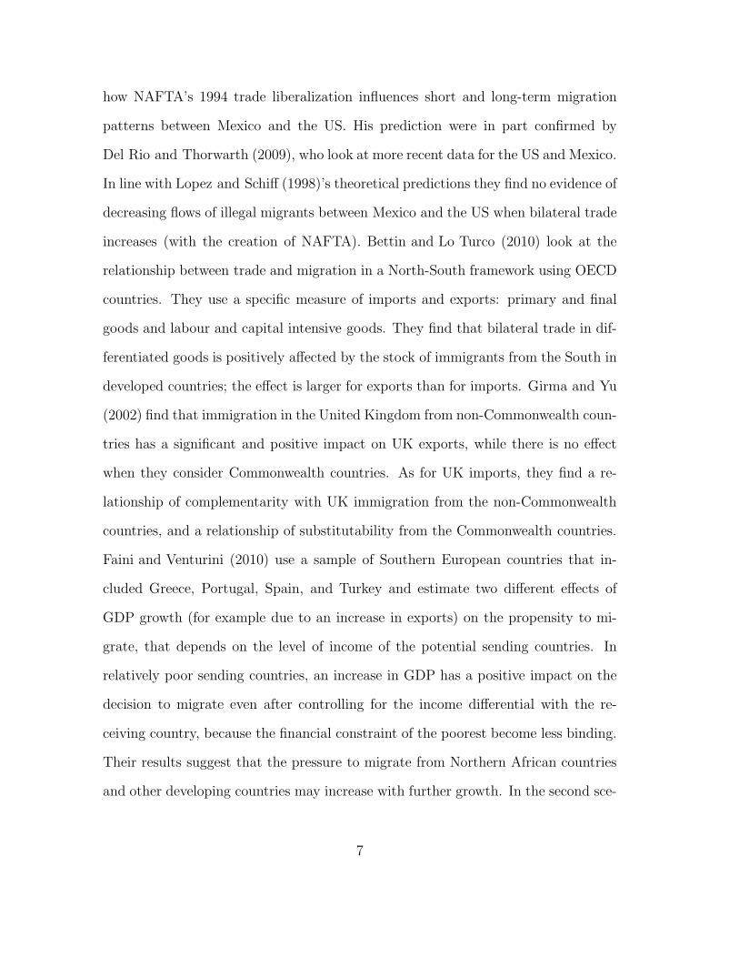
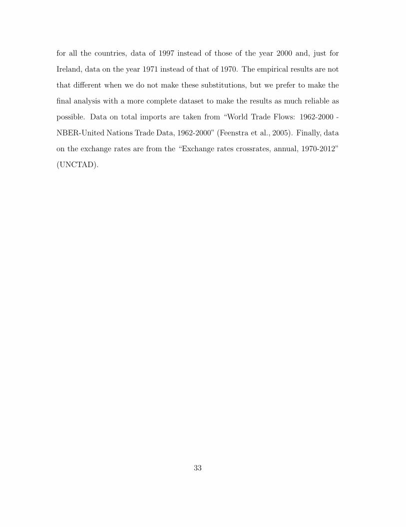
effective in reducing migrations in the short-run. We use bilateral exports and mi-

gration flows from the 12 South Mediterranean countries (Morocco, Algeria, Tunisia,

Egypt, Israel, Jordan, Palestinian Territories, Lebanon, Syria, Turkey, Cyprus and

Malta) to the 15 European Union ones (Belgium, Denmark, Germany, Greece, Spain,

France, Ireland, Italy, Luxembourg, Netherlands, Austria, Portugal, Finland, Swe-

den, United Kingdom) that signed the Euro-Mediterranean partnership over the

period 1970-2000 (Figure 4 in the appendix). In our paper we refer to the EU coun-

tries as “North”, while to the others as “South”.

Quite surprisingly there are no studies that consider the relationship between trade

1The reasons for these exceptions (Algeria, Libya and Malta) are different. In 1973 the Algeriangovernment, after the large migration wave to France in previous decades, and thanks to its naturalresources (oil and gas), decided to prohibit out-migration, which was considered a form of post-colonialism. For the next three decades migration was just driven by French family reunificationschemes (Di Bartolomeo et al., 2010). Libya has recorded more immigration than emigration flows,thanks, again, to its natural resources and the lack of internal labour supply, that attracted peoplefrom Arab countries (Di Bartolomeo et al., 2011). Malta experienced a terrific emigration from1945 to 1979 due to over-population and unemployment, while in the following decades became acountry of destination of migration flows (Plowman, 2010).

3

and migration looking at all the countries of the Euro-Mediterranean partnership,

which represents the EU’s first comprehensive policy for the region and one of its

most ambitious and innovative foreign policy initiatives.

Furthermore, the empirical studies on this topic, that we are going to mention later

in the literature review, disregard the potential reverse causality between trade and

migrations. We go further trying to identify the causal effect of trade on migration.

To this aim we use an instrumental variable approach exploiting information on fac-

tors that are likely to influence the relationship between Southern exporting firms

and Northern importing firms without directly influencing migration. These factors

are the trade tariffs in the destination countries and the exchange rate volatility

between pairs of exporting and importing countries.

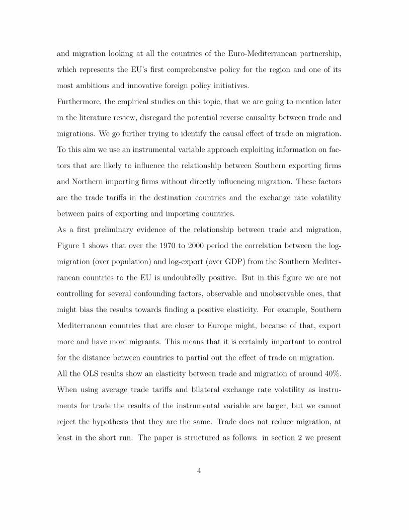
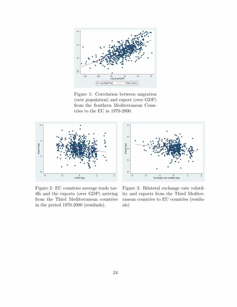
As a first preliminary evidence of the relationship between trade and migration,

Figure 1 shows that over the 1970 to 2000 period the correlation between the log-

migration (over population) and log-export (over GDP) from the Southern Mediter-

ranean countries to the EU is undoubtedly positive. But in this figure we are not

controlling for several confounding factors, observable and unobservable ones, that

might bias the results towards finding a positive elasticity. For example, Southern

Mediterranean countries that are closer to Europe might, because of that, export

more and have more migrants. This means that it is certainly important to control

for the distance between countries to partial out the effect of trade on migration.

All the OLS results show an elasticity between trade and migration of around 40%.

When using average trade tariffs and bilateral exchange rate volatility as instru-

ments for trade the results of the instrumental variable are larger, but we cannot

reject the hypothesis that they are the same. Trade does not reduce migration, at

least in the short run. The paper is structured as follows: in section 2 we present

4

the literature review, in section 3 the empirical strategy, while we show and discuss

the results in section 4. In section 5 we identify the causality using an instrumental

variable approach to cope with the potential endogeneity problem and to measure

the effect of trade on migration. Section 6 is devoted to some robustness checks.

Finally section 7 presents the conclusions and the policy implications.

2 Literature Review

Most of the research on trade and migration focuses on investigating the relationship

of complementarity or substitutability between trade and factor movements (capital

and labour). This relationship has been widely studied at a theoretical level, while

the empirical evidence is rather scarce.

Traditional theory suggests that both should be substitutes. Mundell (1957)

used the Heckscher-Ohlin model to demonstrate that trade and factor movement are

substitutes: countries can either export labour-intensive goods or have their labour

migrate to produce them in the destination country. Similarly, Layard (1992) claims

that the substantial migration pressure from the East and South can be reduced by

exporting capital, and liberalizing trade.

Modern trade theory and extensions of traditional models show that the relation-

ship can also be of complementarity. Several theoretical papers (Markusen, 1983,

Wong, 1983) perturb some of the assumptions underlying the Heckscher-Ohlin model

(e.g. different technologies or scale effects in production), and trade and migration

become complements. The idea is that with migration labour can move where it is

most productive and increase output and exports.

Lopez and Schiff (1998) demonstrates that complementarity is more likely the

higher the migration costs, the tighter the credit constraints of migrants, and the

5

lower the skills and income of potential migrants. It means that opening markets

in the North is more likely to slow down migration from Eastern Europe to the EU

than from Africa to the EU, or from Latin America to the U.S. Furthermore, free

trade may worsen the skill composition of migration from Africa to the EU and from

Latin America to the U.S.

The empirical papers on this subject are quite recent and mainly based on studies

which consider trade and migration flows between a single country and the rest of

the world. Bruder (2004) focuses on “North to North” trade and labour migration

between Germany and some other European country. The findings indicate that

there is a relationship of substitution between trade and foreign labour force. In

particular they find that there isn’t a significant impact of labour migration on

trade, while there is a significantly negative effect of trade on labour migration.

Akkoyunlu and Siliverstovs (2009) investigate whether migration and trade are

complements or substitutes using 1963-2004 data on Turkish migration to Germany.

Cointegration analysis shows that migration and trade are complements for these

two countries. But many other countries signed the Mediterranean agreements. We

are going to use data on all of them.

Collins et al. (1997) try to use a more flexible approach to highlight for which

economies of the “Atlantic community” (plus Australia) between 1870 and 1940

factor mobility and international trade have been complements or substitutes. They

find that they were rarely substitutes and often complements.

Acevedo and Espenshade (1992) and Martin (1993) show that in the short-

to-medium period NAFTA is likely to increase migrations from Mexico to the

United States, but that narrowing the wide economic differentials between the two

countries could substantially reduce the migratory flow. Martin (1993) predicts

6

how NAFTA’s 1994 trade liberalization influences short and long-term migration

patterns between Mexico and the US. His prediction were in part confirmed by

Del Rio and Thorwarth (2009), who look at more recent data for the US and Mexico.

In line with Lopez and Schiff (1998)’s theoretical predictions they find no evidence of

decreasing flows of illegal migrants between Mexico and the US when bilateral trade

increases (with the creation of NAFTA). Bettin and Lo Turco (2010) look at the

relationship between trade and migration in a North-South framework using OECD

countries. They use a specific measure of imports and exports: primary and final

goods and labour and capital intensive goods. They find that bilateral trade in dif-

ferentiated goods is positively affected by the stock of immigrants from the South in

developed countries; the effect is larger for exports than for imports. Girma and Yu

(2002) find that immigration in the United Kingdom from non-Commonwealth coun-

tries has a significant and positive impact on UK exports, while there is no effect

when they consider Commonwealth countries. As for UK imports, they find a re-

lationship of complementarity with UK immigration from the non-Commonwealth

countries, and a relationship of substitutability from the Commonwealth countries.

Faini and Venturini (2010) use a sample of Southern European countries that in-

cluded Greece, Portugal, Spain, and Turkey and estimate two different effects of

GDP growth (for example due to an increase in exports) on the propensity to mi-

grate, that depends on the level of income of the potential sending countries. In

relatively poor sending countries, an increase in GDP has a positive impact on the

decision to migrate even after controlling for the income differential with the re-

ceiving country, because the financial constraint of the poorest become less binding.

Their results suggest that the pressure to migrate from Northern African countries

and other developing countries may increase with further growth. In the second sce-

7

nario, when the sending country is relatively better off (they estimate $4,300 in 1985

prices as a threshold), an increase in income may decrease the migratory pressure.

Overall most studies on “South-North” migration and trade find these to be com-

plements. The problem of all these papers is that they look at simple correlations

and not at causal effects. As mentioned by Gen et al. (2011), just a few papers try

to tackle the problem of endogeneity, focussing on the effect of migration on trade,

rather than on the effect of trade on migration. Furthermore the identification strat-

egy of these papers is not very convincing, as they use the lags of migration as a

instrument for migration under the assumption that past migrant flows are based

on historical networks and ‘well-trodden paths’ rather than current economic con-

ditions. This instrument would not be valid if current trade depends also on past

migrations, violating the assumption of orthogonality between the instrument and

the error term. To the best of our knowledge there are no papers that try to identify

the causal effect of trade on migration. This is exactly the aim of our study.

3 The empirical strategy

3.1 The gravity model

In our paper we adopt the most popular model used to explain international migra-

tion patterns: the gravity model, first introduced by Tinbergen (1962) and Poyhonen

(1963) for bilateral trade2

The theory has been long recognized for its empirical success in explaining dif-

ferent types of flows in economics, such as migration, commuting, shopping trips,

2This model has been borrowed by physics, in particular by the Newton’s law of universalgravitation, which states that the gravitational attraction exerted on an object by a body, decreaseswith the squared distance between the objects attracted and is proportional to the masses of thebodies.

8

tourism, and trade. Furthermore the gravity model has a rather high explanatory

power, which makes it an attractive specification to test the marginal influence of

additional explanatory variables, such as language similarity, colonial ties, exchange

rates, contiguity and trade agreements (Gen et al., 2011). The amount of migra-

tion between two countries is likely to increase in the economic size of the countries

(measured by their GDP) and decreasing in the cost of transportation between them

(measured by geographical distance).

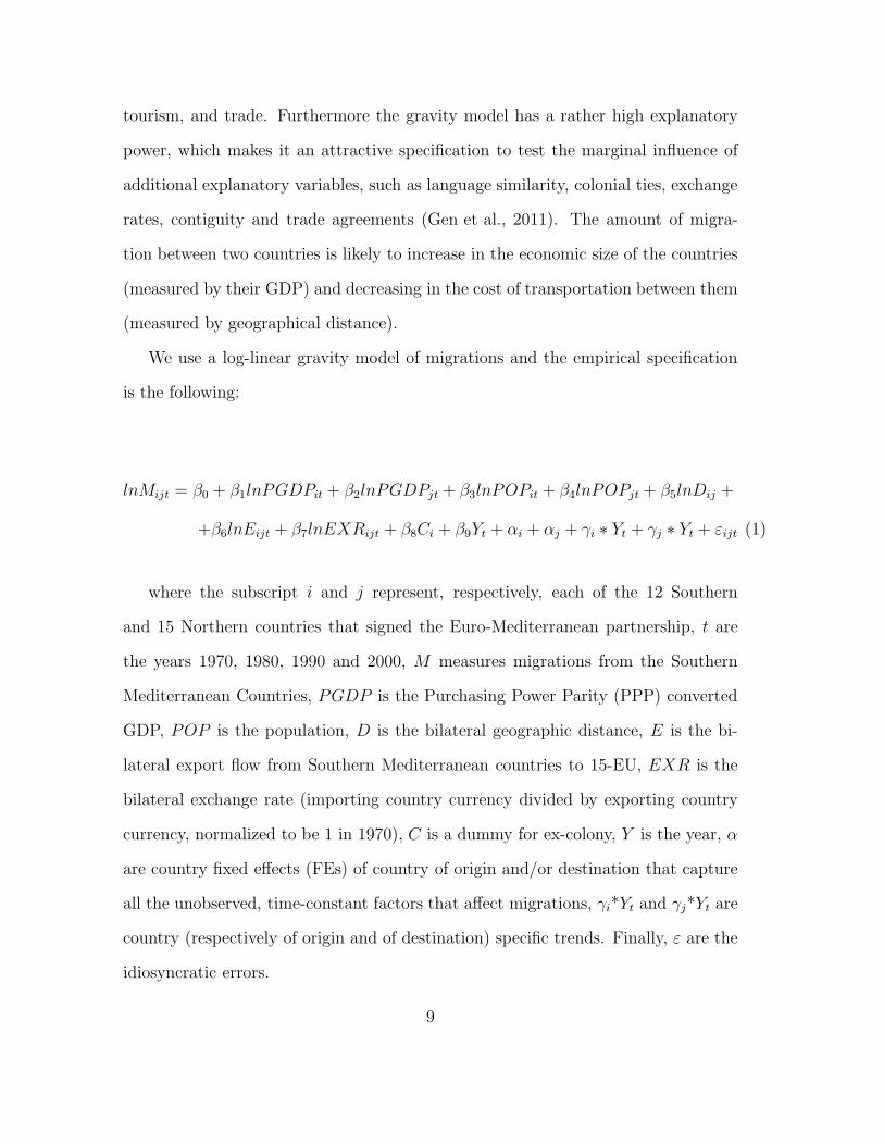
We use a log-linear gravity model of migrations and the empirical specification

is the following:

lnMijt = β0 + β1lnPGDPit + β2lnPGDPjt + β3lnPOPit + β4lnPOPjt + β5lnDij +

+β6lnEijt + β7lnEXRijt + β8Ci + β9Yt + αi + αj + γi ∗ Yt + γj ∗ Yt + εijt (1)

where the subscript i and j represent, respectively, each of the 12 Southern

and 15 Northern countries that signed the Euro-Mediterranean partnership, t are

the years 1970, 1980, 1990 and 2000, M measures migrations from the Southern

Mediterranean Countries, PGDP is the Purchasing Power Parity (PPP) converted

GDP, POP is the population, D is the bilateral geographic distance, E is the bi-

lateral export flow from Southern Mediterranean countries to 15-EU, EXR is the

bilateral exchange rate (importing country currency divided by exporting country

currency, normalized to be 1 in 1970), C is a dummy for ex-colony, Y is the year, α

are country fixed effects (FEs) of country of origin and/or destination that capture

all the unobserved, time-constant factors that affect migrations, γi*Yt and γj*Yt are

country (respectively of origin and of destination) specific trends. Finally, ε are the

idiosyncratic errors.

9

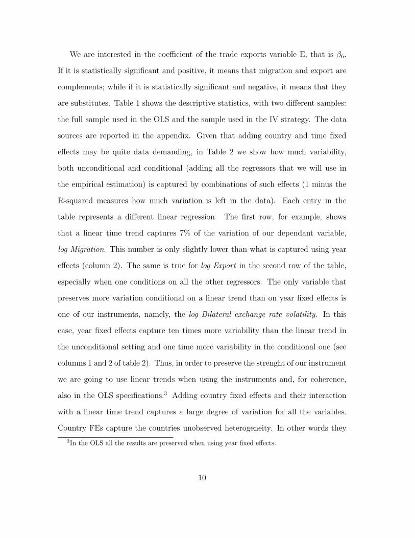
We are interested in the coefficient of the trade exports variable E, that is β6.

If it is statistically significant and positive, it means that migration and export are

complements; while if it is statistically significant and negative, it means that they

are substitutes. Table 1 shows the descriptive statistics, with two different samples:

the full sample used in the OLS and the sample used in the IV strategy. The data

sources are reported in the appendix. Given that adding country and time fixed

effects may be quite data demanding, in Table 2 we show how much variability,

both unconditional and conditional (adding all the regressors that we will use in

the empirical estimation) is captured by combinations of such effects (1 minus the

R-squared measures how much variation is left in the data). Each entry in the

table represents a different linear regression. The first row, for example, shows

that a linear time trend captures 7% of the variation of our dependant variable,

log Migration. This number is only slightly lower than what is captured using year

effects (column 2). The same is true for log Export in the second row of the table,

especially when one conditions on all the other regressors. The only variable that

preserves more variation conditional on a linear trend than on year fixed effects is

one of our instruments, namely, the log Bilateral exchange rate volatility. In this

case, year fixed effects capture ten times more variability than the linear trend in

the unconditional setting and one time more variability in the conditional one (see

columns 1 and 2 of table 2). Thus, in order to preserve the strenght of our instrument

we are going to use linear trends when using the instruments and, for coherence,

also in the OLS specifications.3 Adding country fixed effects and their interaction

with a linear time trend captures a large degree of variation for all the variables.

Country FEs capture the countries unobserved heterogeneity. In other words they

3In the OLS all the results are preserved when using year fixed effects.

10

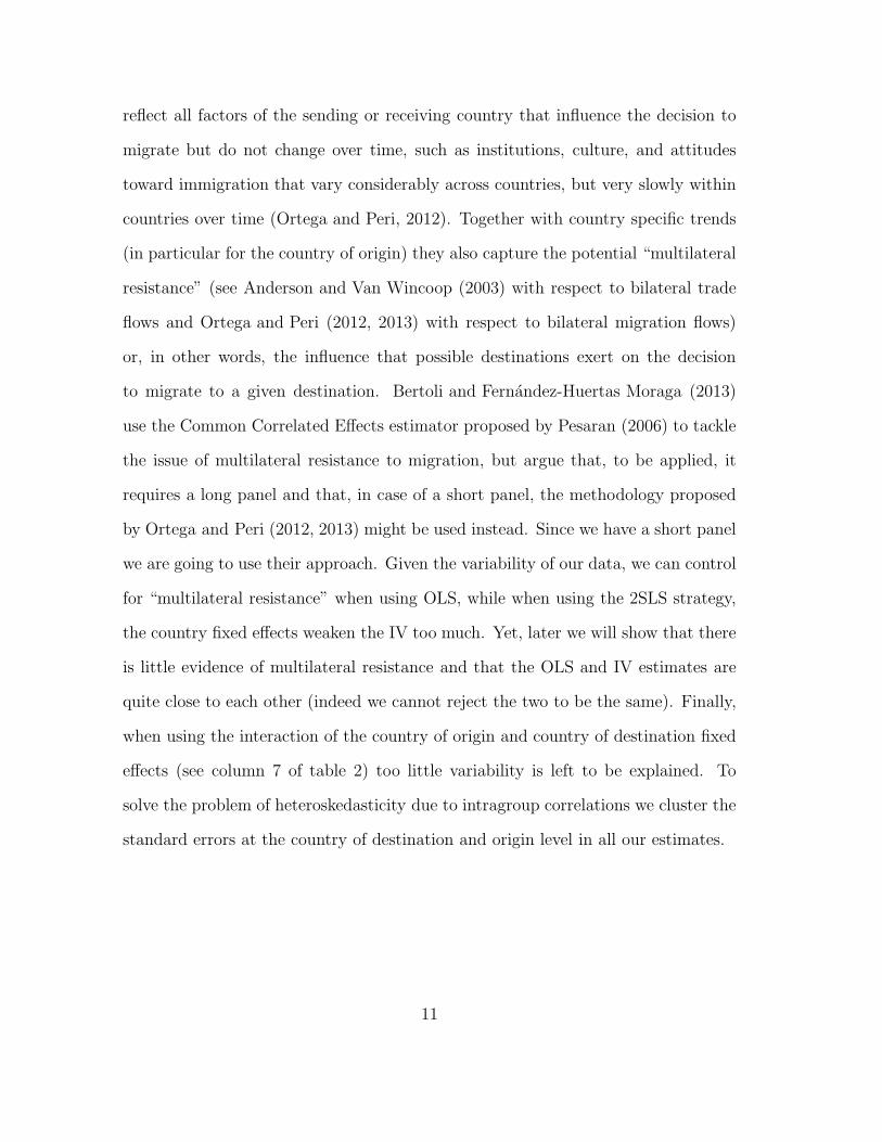
reflect all factors of the sending or receiving country that influence the decision to

migrate but do not change over time, such as institutions, culture, and attitudes

toward immigration that vary considerably across countries, but very slowly within

countries over time (Ortega and Peri, 2012). Together with country specific trends

(in particular for the country of origin) they also capture the potential “multilateral

resistance” (see Anderson and Van Wincoop (2003) with respect to bilateral trade

flows and Ortega and Peri (2012, 2013) with respect to bilateral migration flows)

or, in other words, the influence that possible destinations exert on the decision

to migrate to a given destination. Bertoli and Fernandez-Huertas Moraga (2013)

use the Common Correlated Effects estimator proposed by Pesaran (2006) to tackle

the issue of multilateral resistance to migration, but argue that, to be applied, it

requires a long panel and that, in case of a short panel, the methodology proposed

by Ortega and Peri (2012, 2013) might be used instead. Since we have a short panel

we are going to use their approach. Given the variability of our data, we can control

for “multilateral resistance” when using OLS, while when using the 2SLS strategy,

the country fixed effects weaken the IV too much. Yet, later we will show that there

is little evidence of multilateral resistance and that the OLS and IV estimates are

quite close to each other (indeed we cannot reject the two to be the same). Finally,

when using the interaction of the country of origin and country of destination fixed

effects (see column 7 of table 2) too little variability is left to be explained. To

solve the problem of heteroskedasticity due to intragroup correlations we cluster the

standard errors at the country of destination and origin level in all our estimates.

11

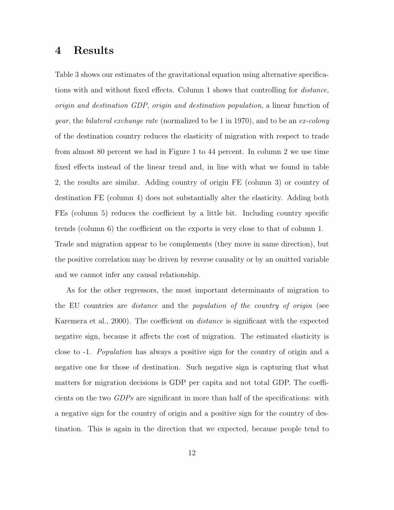
4 Results

Table 3 shows our estimates of the gravitational equation using alternative specifica-

tions with and without fixed effects. Column 1 shows that controlling for distance,

origin and destination GDP, origin and destination population, a linear function of

year, the bilateral exchange rate (normalized to be 1 in 1970), and to be an ex-colony

of the destination country reduces the elasticity of migration with respect to trade

from almost 80 percent we had in Figure 1 to 44 percent. In column 2 we use time

fixed effects instead of the linear trend and, in line with what we found in table

2, the results are similar. Adding country of origin FE (column 3) or country of

destination FE (column 4) does not substantially alter the elasticity. Adding both

FEs (column 5) reduces the coefficient by a little bit. Including country specific

trends (column 6) the coefficient on the exports is very close to that of column 1.

Trade and migration appear to be complements (they move in same direction), but

the positive correlation may be driven by reverse causality or by an omitted variable

and we cannot infer any causal relationship.

As for the other regressors, the most important determinants of migration to

the EU countries are distance and the population of the country of origin (see

Karemera et al., 2000). The coefficient on distance is significant with the expected

negative sign, because it affects the cost of migration. The estimated elasticity is

close to -1. Population has always a positive sign for the country of origin and a

negative one for those of destination. Such negative sign is capturing that what

matters for migration decisions is GDP per capita and not total GDP. The coeffi-

cients on the two GDPs are significant in more than half of the specifications: with

a negative sign for the country of origin and a positive sign for the country of des-

tination. This is again in the direction that we expected, because people tend to

12

migrate from poorer (South Mediterranean shore) to richer countries (EU), where

income opportunities are higher (see Mayda, 2010). The bilateral exchange rates

(normalized to 1970) are negative in all the specifications, but significant in 3 of

them. The reason might be that people decide to migrate to countries where the

exchange rate with their country of origin is low, because the remittance receipts

are larger and, in case of temporary migrations, they can accumulate savings (Yang,

2008). Time is significant (and negative) just for the baseline gravity equation.

Past colonial relationship positively affects the migration flows in all the specifica-

tions we use. South-North migration is positively correlated to South-North exports.

5 Causality

Fixed effect specifications may not be able to capture time varying unobserved het-

erogeneity, and thus be unable to identify the causal mechanism between trade and

migration. As we mentioned before the correlation between the two variables might

due to an omitted variable we do not control for or to reverse causality: migrations

may increase trade. To address the endogeneity problem we adopt a Two Stage

Least Square (2SLS) approach, that uses two different instruments for trade flows,

which are plausibly exogenous with respect to migration: average trade tariffs and

bilateral exchange rate volatility.

Trade tariffs are all levies collected on goods that are entering the country or services

delivered by nonresidents to residents. They include levies imposed for revenue or

protection purposes and determined on a specific or ad valorem basis as long as they

are restricted to imported goods or services. In other words these taxes increase the

13

cost of imported goods, giving an advantage to the domestic producers. We first

collected data on tax revenues on customs and other import duties over GDP and

then data on total imports at country level for all the 15-EU countries. In this

way we calculate the percentage of taxation applied to imports for each country

(from now on we will refer to it as to tariff or trade tariff ). We are going to show

that tariffs predict trade flows, but are they also a valid instrument, meaning that

migration does not depend on tariff other than trough trade? The way tariffs are

measured in this paper make them not only depend on bilateral trade agreements

and international agreements but also on the cost of custom operations. The iden-

tification assumption of this paper is that such an aggregate measure of tariffs does

not depend on migratory flows. In other words, we assume that governments set

overall trade tariffs to influence trade and not migration flows. Suppose EU coun-

tries set bilateral tariffs to influence trade but also migration. In such case one

would like to use the part of tariffs that is set to influence overall trade and not

migration from a specific country as an instrument. A potential measure for such

part would be the tariffs versus all the non-Third Mediterranean countries. Unfor-

tunately data bilateral tariffs are not available back in time, but since we are using

an imports-weighted aggregate measure of tariffs, such aggregate is going to be very

similar to the measure that excludes these countries as long as imports from Third

Mediterranean Countries are small with respect to all the other imports. Indeed,

their exports to EU countries represent between 0.04 percent (Portugal) and 0.23

percent (Italy) of total imports to these countries. Table 4 shows the trade tariffs

of the EU countries in the years 1970, 1980, 1990 and 1997. We use 1997 because

it’s the first year going back from the 2000 with a complete and coherent measure-

ment for the countries we look at. Note that there is a decreasing trend for tariffs

14

from 1970 to 1997 for all the EU countries. The most dramatic variation is from

1970 to 1980 (on average -72%). This is not surprising because during the oil and

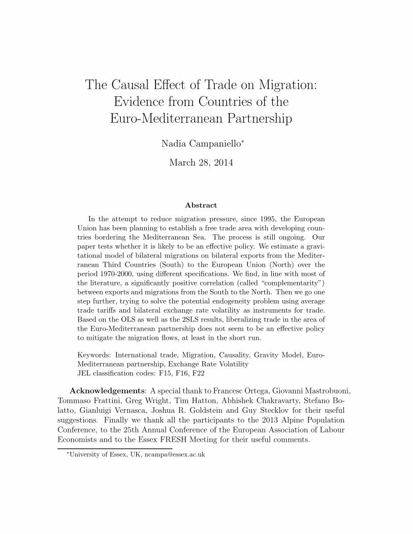
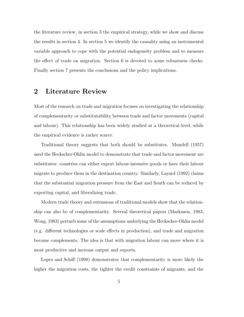
financial crises of the 1970s protectionism was widespread in world trade. In Figure

2 we plot tariffs of European countries (the instrument) against their imports from

Third Mediterranean partners (the instrumented variable) after conditioning on all

the regressors used later in the main specification (Column 1 of Table 3). There is

clearly a negative correlation between the two variables. The coefficient in a simple

bivariate regression is equal to 0.48.

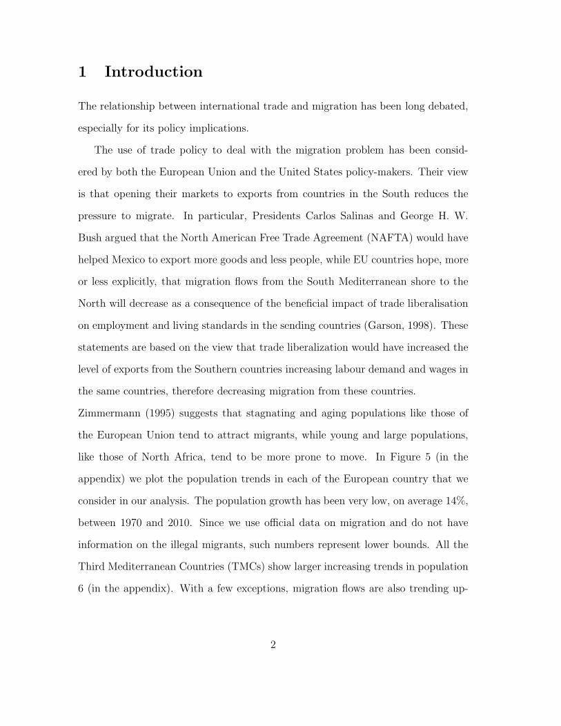
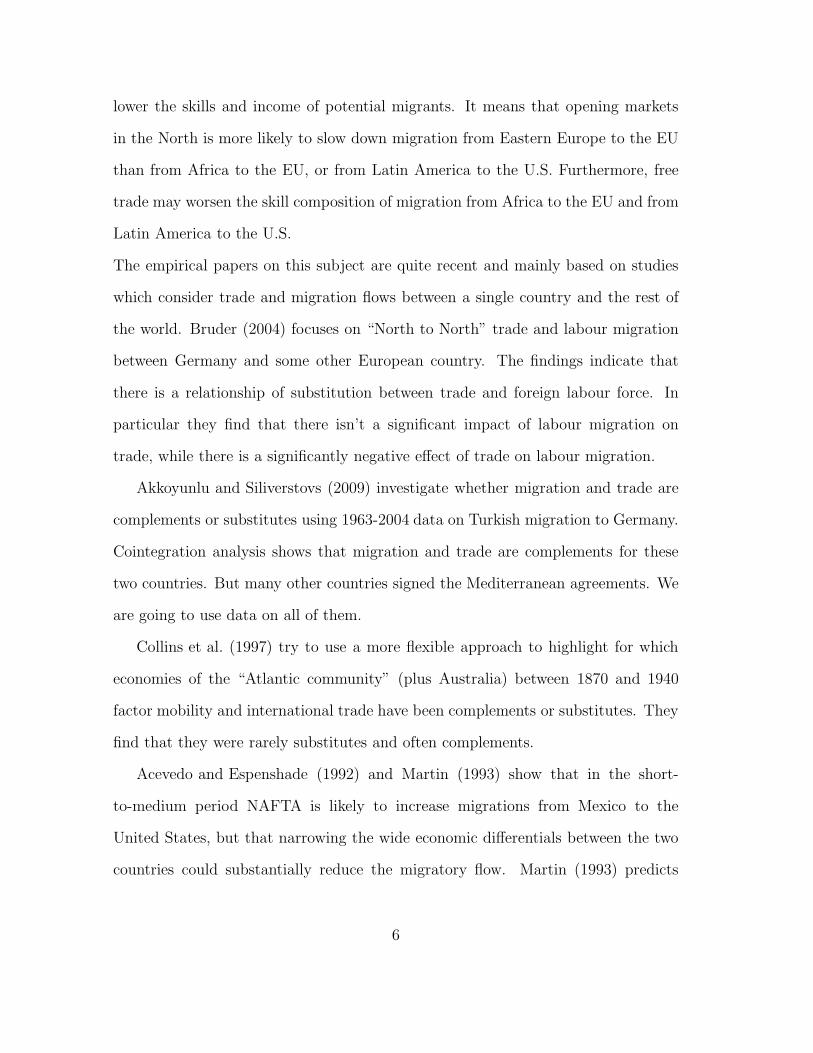
As a second instrumental variable we use the bilateral exchange rate volatility. There

is consistent evidence in the literature that exchange rate volatility negatively af-

fects bilateral trade (Byrne et al., 2008, Chowdhury, 1993, Dell’Ariccia, 1998, Pozo,

1992). The argument is that by increasing uncertainty and risk, if hedging is im-

possible or costly, risk-averse agents are discouraged to engage in trade, especially

since trade relations between exporting and importing firms are bound to persist

over time. Expectations of future volatility are based on past trends and for this

reason we consider a period of 10 years. We normalize the annual bilateral exchange

rates over a 10-year period to the exchange rate of the first year of each decennial

period (1970, 1980, 1990, 2000) and then calculate the variance. In figure 3 we plot

exports against exchange rate volatility after conditioning on all the other regres-

sors used later in the main specification (Column 1 of Table 3). There is a clear

negative correlation between the two variables. While there is no empirical evidence

that tariffs are set in order to control migration and that the second moment of

exchange rates determines migratory flows (for example none of the papers that

we are aware of control for the second moment of exchange rate when explaining

migratory flows), having two instruments allows us to perform an overidentification

15

test. Even if nobody has ever made this point before, one might argue that immi-

grants might choose the country of destination taking the variability of the exchange

rate into consideration in order to smooth potential future remittances and that the

average trade tariffs are set taking bilateral migratory flows into account. If this

was the case, the fact that we cannot reject the overidentification test means that

the biases introduced by the two instruments would have to be the same, which is

arguably unlikely. The results from the first stage are shown in Table 5. Table 6

shows the results of the IV (2SLS) estimation using both the bilateral exchange rate

volatility and average trade tariffs as instruments. The first stage F-statistic is equal

to 19.251, which is above the rule of thumb value of 10 indicated by the literature

on weak instruments (Bound et al., 1995, Stock and Yogo, 2002). Then we use the

J-statistic to test the exogeneity and we find a p-value equal to 0.674.

Finally, we use the Hausman t statistic to compare OLS and 2SLS estimates of the

coefficient on exports finding no evidence of endogeneity (the p-value is equal to

0.43). The results that we find with the 2SLS are in line with those of the OLS.

In particular the coefficient of interest, that on exports, is significant and positive.

Note that in the IV there is no variation left after controlling for the FEs (see table

2), but adding those FEs change the OLS estimates very little, suggesting that the

bias is small and is likely to be small for the IV as well. Moreover, as already pointed

out, the estimate based on the IV specification is not statistically different from the

model that assumes that trade is exogenous to migration. To conclude, exports,

at least in the short run, do not seem to mitigate the migration pressure, but to

encourage it.

16

6 Robustness checks

In this section we perform different robustness checks to be sure that our results

are not biased by the particular specification we used. First of all we run the

regressions using a Poisson estimator, as suggested by Silva and Tenreyro (2006):

under heteroskedasticity, the parameters of log-linearized models estimated by OLS

lead to biased estimates of the true elasticities. We find a positive and significant

semi-elasticity of 1.297 on the coefficient export. As a second robustness check,

we introduce as a regressor in the OLS the sum of all exports from a given Third

Mediterranean Country i to all European Union countries excluding country j, al-

lowing for an indirect effect on migrations towards the European country j. We find

a higher coefficient compared to that of the baseline specification of the OLS, equal

to 0.526 on the variable export.

One could argue that since we are controlling for GDP of the country of origin, the

elasticity is bound to be positive. Migration flows might decrease when countries

export more and become richer, but controlling for country of origin GDP we are

shutting off such a channel. This is the reason why in the third robustness we sub-

tract exports from GDP. In this way an increase in export determines a one to one

increase in GDP. Doing so barely changes the results. An alternative way to com-

pletely get rid of GDP is not to control for country of origin GDP. The coefficient

on the variable export is the same as in the main specification.

Another objection could be related to the inclusion of Israel and Malta among the

Southern countries. Indeed their economic conditions are very similar to those of the

EU countries. For this reason we run the regressions without Malta and Israel and

we find very similar results. As shown in table 7 in all of these robustness checks we

find a positive and significant relationship between trade and migration. All these

17

results are in line with those of the main analysis.

7 Conclusions

In 1995 European Union policymakers decided to establish a free trade area in the

region of the Euro-Mediterranean partnership hoping that such policy would in-

crease trade (in particular exports from the TMCs) and that, in turn, trade would

lead to a reduction in migration. The process is still ongoing. Policy makers as-

sumed that trade has a negative effect on migrations. In our paper we find, looking

at the period 1970-2000, that the effect is the opposite: exports increase migration.

Such a conclusion is reached not just looking at simple correlations between trade

and migration, but trying to solve the potential endogeneity problem using an in-

strumental variable approach. In particular we adopt a 2SLS approach that use

average trade tariffs and bilateral exchange rate volatility as instruments for trade

flows. We find that increasing trade is likely to increase the number of migrants from

Southern Mediterranean to the European Union. These results might be driven by

the creation of links between the countries involved in trade: migrants need these

links to enter the receiving country. For example Italy sets immigration quotas that

can only be filled by migrants with a job offer in Italy. We just conclude saying

that EU policymakers should not consider free trade as a valid policy to decrease

migrations from the Third Mediterranean countries to Europe, at least in the short

run. Due to data limitations it is impossible to analyze whether such patterns can

be reversed in the long-run, when Southern countries will have converged to the

economic development of Northern ones (see Faini and Venturini, 2010).

18

References

D. Acevedo and T.J. Espenshade. Implications of a North American Free Trade

Agreement for Mexican migration into the United States. The Population and

Development Review, pages 729–744, 1992.

S. Akkoyunlu and B. Siliverstovs. Migration and Trade: Complements or Substi-

tutes? Evidence from Turkish Migration to Germany. Emerging Markets Finance

and Trade, 45(5):47–61, 2009.

James E Anderson and Eric Van Wincoop. Gravity with gravitas: A solution to the

border puzzle. The American Economic Review, 93(1):170–192, 2003.

Simone Bertoli and Jesus Fernandez-Huertas Moraga. Multilateral resistance to

migration. Journal of Development Economics, 102:79–100, 2013.

G. Bettin and A. Lo Turco. A Cross Country View on South-North Migration and

Trade. Dissecting the Channels. Working Paper Universita della Calabria, 10(15):

35, 2010.

J. Bound, D.A. Jaeger, and R.M. Baker. Problems with instrumental variables

estimation when the correlation between the instruments and the endogeneous

explanatory variable is weak. Journal of the American Statistical Association,

pages 443–450, 1995.

J. Bruder. Are trade and migration substitutes or complements? The case of Ger-

many, 1970-1998. European Trade Study Group, pages 9–11, 2004.

Joseph P Byrne, Julia Darby, and Ronald MacDonald. Us trade and exchange rate

19

volatility: A real sectoral bilateral analysis. Journal of macroeconomics, 30(1):

238–259, 2008.

Abdur Chowdhury. Does exchange rate variability depress trade flows? evidence

from error correction models. Review of Economics and Statistics, 1993.

W.J. Collins, K.H. O’Rourke, and J. Williamson. Were trade and factor mobility

substitutes in history? Technical report, National Bureau of Economic Research,

1997.

A.M. Del Rio and S. Thorwarth. Tomatoes or tomato pickers? Free trade and

migration between Mexico and the United States. Journal of Applied Economics,

12(1):109–134, 2009.

Giovanni Dell’Ariccia. Exchange Rate Fluctuations and Trade Flows-Evidence from

the European Union. International Monetary Fund, 1998.

A. Di Bartolomeo, T. Jaulin, and D. Perrin. Algeria. The Demographic-Economic

Framework of Migration. The Legal Framework of Migration. The Socio-Political

Framework of Migration. Technical report, Robert Schuman Centre for Advanced

Studies, December 2010.

A. Di Bartolomeo, T. Jaulin, and D. Perrin. Libya. The Demographic-Economic

Framework of Migration. The Legal Framework of Migration. The Socio-Political

Framework of Migration. Technical report, Robert Schuman Centre for Advanced

Studies, June 2011.

R. Faini and A. Venturini. Development and migration: Lessons from southern

europe. In Frontiers of Economics and Globalization, volume 8, chapter 5. Emerald

Group Publishing Limited, 2010.

20

R. C. Feenstra, R. E. Lipsey, H. Deng, A. C. Ma, and H. Mo. World trade flows:

1962-2000. NBER Working Paper, 2005.

J.P. Garson. Opening Mediterranean Trade and Migration. OECD OBSERVER,

pages 21–24, 1998.

M. Gen, M. Gheasi, P. Nijkamp, and J. Poot. The impact of immigration on inter-

national trade: a meta-analysis. Norface Discussion Paper Series, 2011.

S. Girma and Z. Yu. The link between immigration and trade: Evidence from the

United Kingdom. Review of World Economics, 138(1):115–130, 2002.

D. Karemera, V.I. Oguledo, and B. Davis. A gravity model analysis of international

migration to North America. Applied Economics, 32(13):1745–1755, 2000.

P.R.G. Layard. East-West migration: the alternatives. The MIT Press, 1992.

Ramon Lopez and Maurice Schiff. Migration and the skill composition of the labor

force: The impact of trade liberalization in ldcs. Canadian Journal of Economics,

31:318–336, May 1998.

J.R. Markusen. Factor movements and commodity trade as complements. Journal

of International Economics, 14(3-4):341–356, 1983.

P.L. Martin. Trade and migration: Nafta and agriculture. Technical report, Policy

Analysis in International Economics, Washington D.C., 1993.

A.M. Mayda. International migration: A panel data analysis of the determinants of

bilateral flows. Journal of Population Economics, 23(4):1249–1274, 2010.

R.A. Mundell. International trade and factor mobility. The American Economic

Review, 47(3):321–335, 1957.

21

Francesc Ortega and Giovanni Peri. The effect of trade and migration on income.

Technical report, National Bureau of Economic Research, 2012.

Francesc Ortega and Giovanni Peri. The effect of income and immigration policies

on international migration. Migration Studies, 1(1):47–74, 2013.

M Hashem Pesaran. Estimation and inference in large heterogeneous panels with a

multifactor error structure. Econometrica, 74(4):967–1012, 2006.

D. H. Plowman. A Fragment of the Maltese Exodus: Child Migration to Australia

1953-1965. Journal of Maltese History, 2(1), 2010.

P. Poyhonen. A tentative model for the volume of trade between countries.

Weltwirtschaftliches Archiv., 90(1):93–99, 1963.

Susan Pozo. Conditional exchange-rate volatility and the volume of international

trade: evidence from the early 1900s. The Review of Economics and Statistics,

74(2):325–29, 1992.

JMC Santos Silva and Silvana Tenreyro. The log of gravity. The Review of Eco-

nomics and Statistics, 88(4):641–658, 2006.

J.H. Stock and M. Yogo. Testing for weak instruments in linear IV regression.

Technical report, National Bureau of Economic Research, 2002.

J. Tinbergen. Shaping the world economy. suggestions for an international economic

policy. Technical report, Twentieth Century Fund, New York, 1962.

K.Y. Wong. On choosing among trade in goods and international capital and labor

mobility: A theoretical analysis. Journal of International Economics, 14:223–250,

1983.

22

Dean Yang. International migration, remittances and household investment: Ev-

idence from philippine migrants’ exchange rate shocks. The Economic Journal,

118(528):591–630, 2008.

K.F. Zimmermann. Tackling the european migration problem. The Journal of

Economic Perspectives, 9(2):45–62, 1995.

23

−10

−5

05

−12 −10 −8 −6 −4 −2Log (Exp/GDP)

Log (Migr/Pop) Fitted values

Figure 1: Correlation between migration(over population) and export (over GDP)from the Southern Mediterranean Coun-tries to the EU in 1970-2000.

−3

−1

13

Exp

ort (

log)

−2 −1 0 1 2Tariffs (log)

Figure 2: EU countries average trade tar-iffs and the exports (over GDP) arrivingfrom the Third Mediterranean countriesin the period 1970-2000 (residuals).

−4

−2

02

4E

xpor

t (lo

g)

−3 −2 −1 0 1 2Exchange rate volatility (log)

Figure 3: Bilateral exchange rate volatil-ity and exports from the Third Mediter-ranean countries to EU countries (residu-als)

24

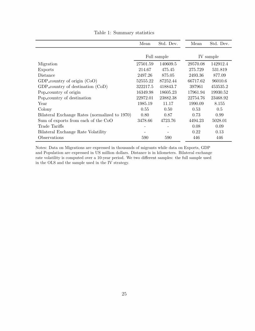
Table 1: Summary statistics

Mean Std. Dev. Mean Std. Dev.

Full sample IV sample

Migration 27501.59 140609.5 29570.08 142912.4Exports 214.67 475.45 275.729 531.819Distance 2497.26 875.05 2493.36 877.09GDP country of origin (CoO) 52555.22 87252.44 66717.62 96010.6GDP country of destination (CoD) 322217.5 418843.7 397961 453535.2Pop country of origin 16349.98 18605.23 17961.94 19930.52Pop country of destination 22972.01 23882.38 22754.76 23468.92Year 1985.19 11.17 1990.09 8.155Colony 0.55 0.50 0.53 0.5Bilateral Exchange Rates (normalized to 1970) 0.80 0.87 0.73 0.99Sum of exports from each of the CoO 3478.66 4723.76 4494.23 5028.01Trade Tariffs - - 0.08 0.09Bilateral Exchange Rate Volatility - - 0.22 0.13Observations 590 590 446 446

Notes: Data on Migrations are expressed in thousands of migrants while data on Exports, GDPand Population are expressed in US million dollars. Distance is in kilometers. Bilateral exchangerate volatility is computed over a 10-year period. We two different samples: the full sample usedin the OLS and the sample used in the IV strategy.

25

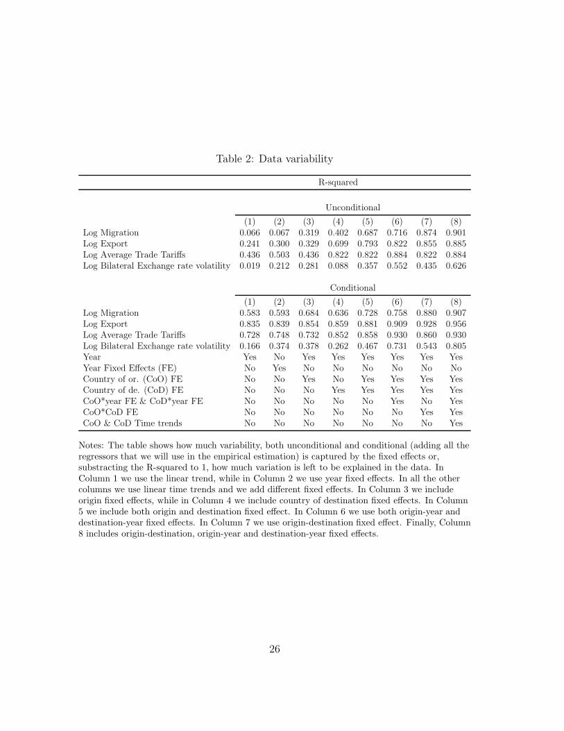
Table 2: Data variability

R-squared

Unconditional

(1) (2) (3) (4) (5) (6) (7) (8)Log Migration 0.066 0.067 0.319 0.402 0.687 0.716 0.874 0.901Log Export 0.241 0.300 0.329 0.699 0.793 0.822 0.855 0.885Log Average Trade Tariffs 0.436 0.503 0.436 0.822 0.822 0.884 0.822 0.884Log Bilateral Exchange rate volatility 0.019 0.212 0.281 0.088 0.357 0.552 0.435 0.626

Conditional

(1) (2) (3) (4) (5) (6) (7) (8)Log Migration 0.583 0.593 0.684 0.636 0.728 0.758 0.880 0.907Log Export 0.835 0.839 0.854 0.859 0.881 0.909 0.928 0.956Log Average Trade Tariffs 0.728 0.748 0.732 0.852 0.858 0.930 0.860 0.930Log Bilateral Exchange rate volatility 0.166 0.374 0.378 0.262 0.467 0.731 0.543 0.805Year Yes No Yes Yes Yes Yes Yes YesYear Fixed Effects (FE) No Yes No No No No No NoCountry of or. (CoO) FE No No Yes No Yes Yes Yes YesCountry of de. (CoD) FE No No No Yes Yes Yes Yes YesCoO*year FE & CoD*year FE No No No No No Yes No YesCoO*CoD FE No No No No No No Yes YesCoO & CoD Time trends No No No No No No No Yes

Notes: The table shows how much variability, both unconditional and conditional (adding all theregressors that we will use in the empirical estimation) is captured by the fixed effects or,substracting the R-squared to 1, how much variation is left to be explained in the data. InColumn 1 we use the linear trend, while in Column 2 we use year fixed effects. In all the othercolumns we use linear time trends and we add different fixed effects. In Column 3 we includeorigin fixed effects, while in Column 4 we include country of destination fixed effects. In Column5 we include both origin and destination fixed effect. In Column 6 we use both origin-year anddestination-year fixed effects. In Column 7 we use origin-destination fixed effect. Finally, Column8 includes origin-destination, origin-year and destination-year fixed effects.

26

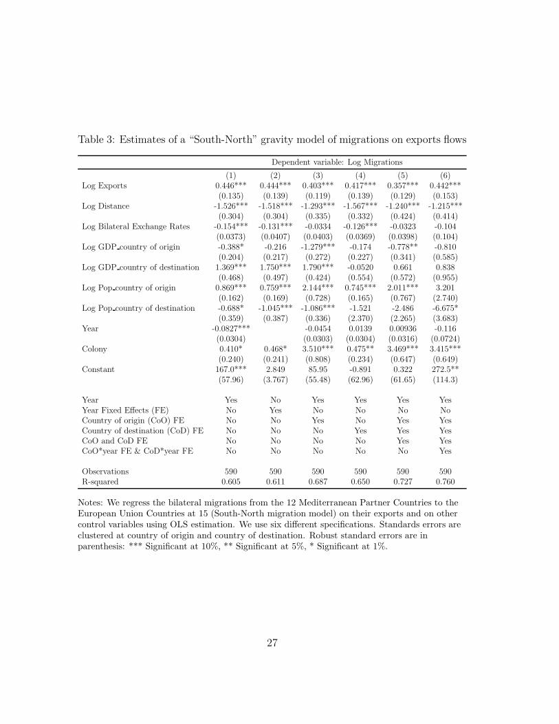
Table 3: Estimates of a “South-North” gravity model of migrations on exports flows

Dependent variable: Log Migrations

(1) (2) (3) (4) (5) (6)Log Exports 0.446*** 0.444*** 0.403*** 0.417*** 0.357*** 0.442***

(0.135) (0.139) (0.119) (0.139) (0.129) (0.153)Log Distance -1.526*** -1.518*** -1.293*** -1.567*** -1.240*** -1.215***

(0.304) (0.304) (0.335) (0.332) (0.424) (0.414)Log Bilateral Exchange Rates -0.154*** -0.131*** -0.0334 -0.126*** -0.0323 -0.104

(0.0373) (0.0407) (0.0403) (0.0369) (0.0398) (0.104)Log GDP country of origin -0.388* -0.216 -1.279*** -0.174 -0.778** -0.810

(0.204) (0.217) (0.272) (0.227) (0.341) (0.585)Log GDP country of destination 1.369*** 1.750*** 1.790*** -0.0520 0.661 0.838

(0.468) (0.497) (0.424) (0.554) (0.572) (0.955)Log Pop country of origin 0.869*** 0.759*** 2.144*** 0.745*** 2.011*** 3.201

(0.162) (0.169) (0.728) (0.165) (0.767) (2.740)Log Pop country of destination -0.688* -1.045*** -1.086*** -1.521 -2.486 -6.675*

(0.359) (0.387) (0.336) (2.370) (2.265) (3.683)Year -0.0827*** -0.0454 0.0139 0.00936 -0.116

(0.0304) (0.0303) (0.0304) (0.0316) (0.0724)Colony 0.410* 0.468* 3.510*** 0.475** 3.469*** 3.415***

(0.240) (0.241) (0.808) (0.234) (0.647) (0.649)Constant 167.0*** 2.849 85.95 -0.891 0.322 272.5**

(57.96) (3.767) (55.48) (62.96) (61.65) (114.3)

Year Yes No Yes Yes Yes YesYear Fixed Effects (FE) No Yes No No No NoCountry of origin (CoO) FE No No Yes No Yes YesCountry of destination (CoD) FE No No No Yes Yes YesCoO and CoD FE No No No No Yes YesCoO*year FE & CoD*year FE No No No No No Yes

Observations 590 590 590 590 590 590R-squared 0.605 0.611 0.687 0.650 0.727 0.760

Notes: We regress the bilateral migrations from the 12 Mediterranean Partner Countries to theEuropean Union Countries at 15 (South-North migration model) on their exports and on othercontrol variables using OLS estimation. We use six different specifications. Standards errors areclustered at country of origin and country of destination. Robust standard errors are inparenthesis: *** Significant at 10%, ** Significant at 5%, * Significant at 1%.

27

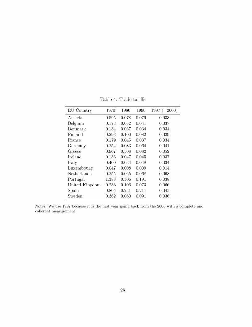
Table 4: Trade tariffs

EU Country 1970 1980 1990 1997 (=2000)

Austria 0.595 0.078 0.079 0.033Belgium 0.178 0.052 0.041 0.037Denmark 0.134 0.037 0.034 0.034Finland 0.293 0.100 0.082 0.029France 0.179 0.045 0.037 0.034Germany 0.254 0.083 0.064 0.041Greece 0.967 0.508 0.082 0.052Ireland 0.136 0.047 0.045 0.037Italy 0.400 0.034 0.048 0.034Luxembourg 0.047 0.008 0.009 0.014Netherlands 0.255 0.065 0.068 0.068Portugal 1.388 0.306 0.191 0.038United Kingdom 0.233 0.106 0.073 0.066Spain 0.805 0.231 0.211 0.045Sweden 0.362 0.060 0.091 0.036

Notes: We use 1997 because it is the first year going back from the 2000 with a complete andcoherent measurement

28

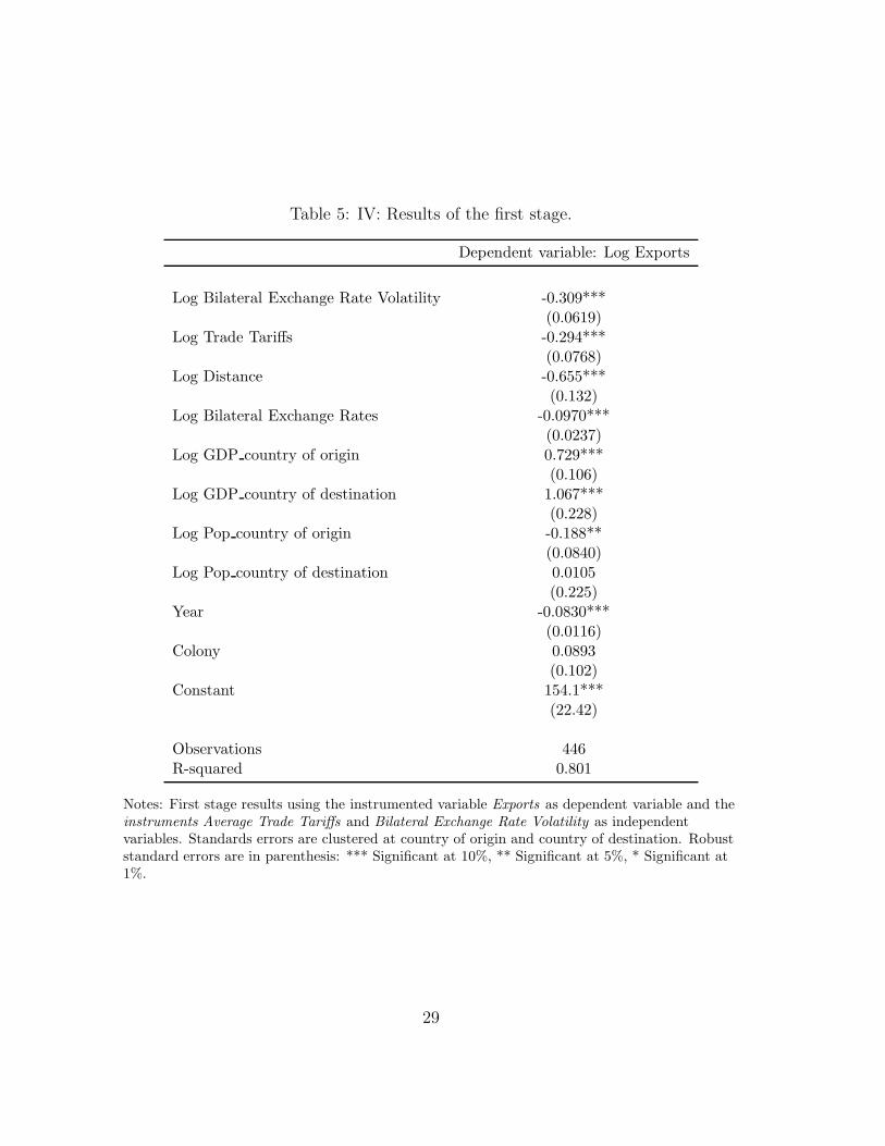
Table 5: IV: Results of the first stage.

Dependent variable: Log Exports

Log Bilateral Exchange Rate Volatility -0.309***(0.0619)

Log Trade Tariffs -0.294***(0.0768)

Log Distance -0.655***(0.132)

Log Bilateral Exchange Rates -0.0970***(0.0237)

Log GDP country of origin 0.729***(0.106)

Log GDP country of destination 1.067***(0.228)

Log Pop country of origin -0.188**(0.0840)

Log Pop country of destination 0.0105(0.225)

Year -0.0830***(0.0116)

Colony 0.0893(0.102)

Constant 154.1***(22.42)

Observations 446R-squared 0.801

Notes: First stage results using the instrumented variable Exports as dependent variable and theinstruments Average Trade Tariffs and Bilateral Exchange Rate Volatility as independentvariables. Standards errors are clustered at country of origin and country of destination. Robuststandard errors are in parenthesis: *** Significant at 10%, ** Significant at 5%, * Significant at1%.

29

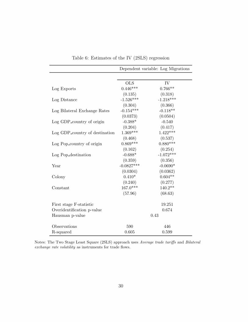
Table 6: Estimates of the IV (2SLS) regression

Dependent variable: Log Migrations

OLS IVLog Exports 0.446*** 0.766**

(0.135) (0.318)Log Distance -1.526*** -1.218***

(0.304) (0.366)Log Bilateral Exchange Rates -0.154*** -0.118**

(0.0373) (0.0504)Log GDP country of origin -0.388* -0.540

(0.204) (0.417)Log GDP country of destination 1.369*** 1.422***

(0.468) (0.537)Log Pop country of origin 0.869*** 0.880***

(0.162) (0.254)Log Pop destination -0.688* -1.072***

(0.359) (0.356)Year -0.0827*** -0.0690*

(0.0304) (0.0362)Colony 0.410* 0.604**

(0.240) (0.277)Constant 167.0*** 140.2**

(57.96) (68.63)

First stage F-statistic 19.251Overidentification p-value 0.674Hausman p-value 0.43

Observations 590 446R-squared 0.605 0.599

Notes: The Two Stage Least Square (2SLS) approach uses Average trade tariffs and Bilateral

exchange rate volatility as instruments for trade flows.

30

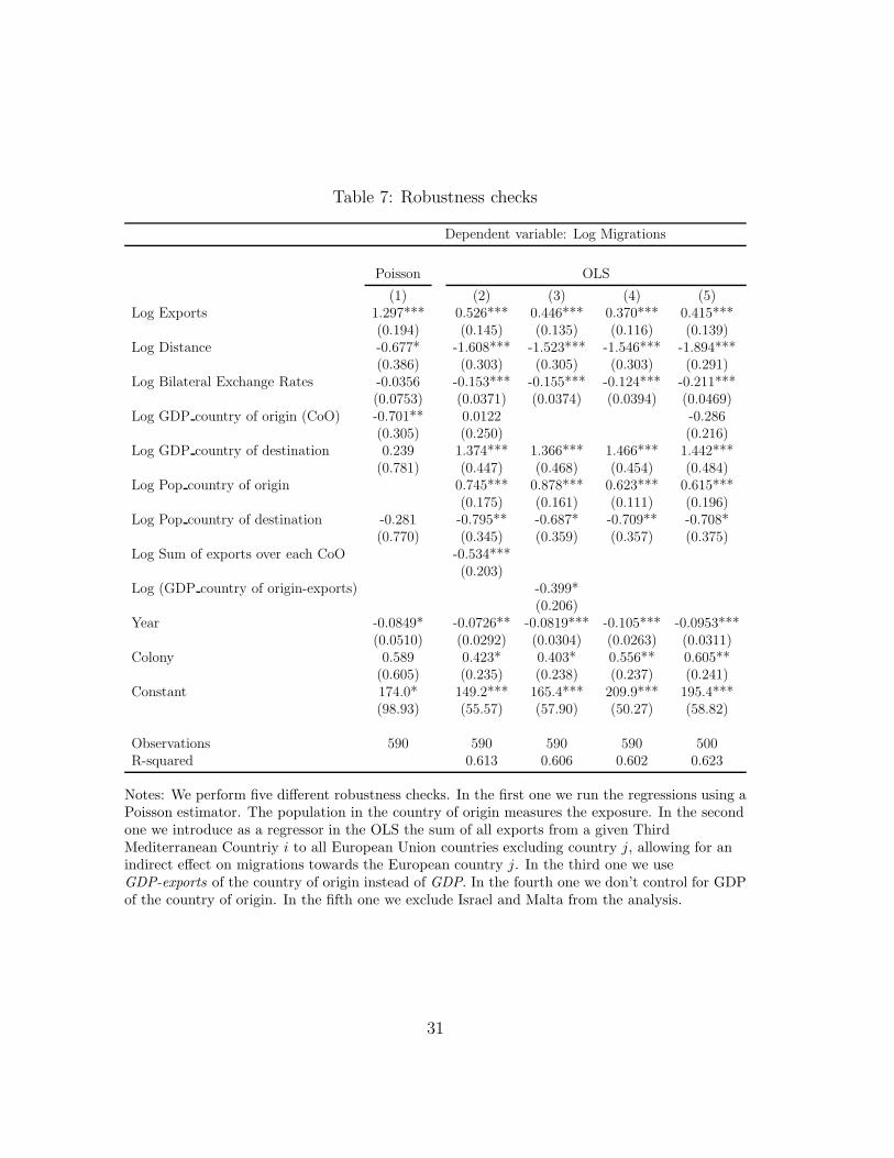
Table 7: Robustness checks

Dependent variable: Log Migrations

Poisson OLS

(1) (2) (3) (4) (5)Log Exports 1.297*** 0.526*** 0.446*** 0.370*** 0.415***

(0.194) (0.145) (0.135) (0.116) (0.139)Log Distance -0.677* -1.608*** -1.523*** -1.546*** -1.894***

(0.386) (0.303) (0.305) (0.303) (0.291)Log Bilateral Exchange Rates -0.0356 -0.153*** -0.155*** -0.124*** -0.211***

(0.0753) (0.0371) (0.0374) (0.0394) (0.0469)Log GDP country of origin (CoO) -0.701** 0.0122 -0.286

(0.305) (0.250) (0.216)Log GDP country of destination 0.239 1.374*** 1.366*** 1.466*** 1.442***

(0.781) (0.447) (0.468) (0.454) (0.484)Log Pop country of origin 0.745*** 0.878*** 0.623*** 0.615***

(0.175) (0.161) (0.111) (0.196)Log Pop country of destination -0.281 -0.795** -0.687* -0.709** -0.708*

(0.770) (0.345) (0.359) (0.357) (0.375)Log Sum of exports over each CoO -0.534***

(0.203)Log (GDP country of origin-exports) -0.399*

(0.206)Year -0.0849* -0.0726** -0.0819*** -0.105*** -0.0953***

(0.0510) (0.0292) (0.0304) (0.0263) (0.0311)Colony 0.589 0.423* 0.403* 0.556** 0.605**

(0.605) (0.235) (0.238) (0.237) (0.241)Constant 174.0* 149.2*** 165.4*** 209.9*** 195.4***

(98.93) (55.57) (57.90) (50.27) (58.82)

Observations 590 590 590 590 500R-squared 0.613 0.606 0.602 0.623

Notes: We perform five different robustness checks. In the first one we run the regressions using aPoisson estimator. The population in the country of origin measures the exposure. In the secondone we introduce as a regressor in the OLS the sum of all exports from a given ThirdMediterranean Countriy i to all European Union countries excluding country j, allowing for anindirect effect on migrations towards the European country j. In the third one we useGDP-exports of the country of origin instead of GDP. In the fourth one we don’t control for GDPof the country of origin. In the fifth one we exclude Israel and Malta from the analysis.

31

A Data sources

In our research we focus on those countries that took part to the Barcelona process

with just a couple of exceptions: the Palestinian Authority and Libya. Although the

former jointed the partnership, it has not been included in the analysis because the

International Monetary Fund (IMF), that collects data on national bilateral trade in

the “Direction of Trade Statistics” (DOTS), has no statistics on this country; as for

the latter it is included in our research both for its dramatic economic and political

importance in the region and because it belongs to the Union for the Mediterranean,

which is the institutional evolution of the Euro-Mediterranean Partnership. Because

of data limitations we use decennial data: 1970, 1980, 1990 and 2000. Data on

national bilateral trade are expressed in US million dollars using the “Dyadic trade

data” (the Inter-University Consortium for the Political and Social Research).

Data on migrations, available every 10 years, are from “Global Bilateral Migra-

tion Database” (The World Bank) and are expressed in thousands of migrants.

Data on the bilateral distance, contiguity and language come from the “Geodist”

database (Centre d’etudes prospectives et d’informations inter-nationales) and are

in kilometers.

Data on Purchasing Power Parity converted GDP and on population are taken

from the “Penn World Table Version 7.0” (Center for International Comparisons of

Production, Income and Prices at the University of Pennsylvania) and are expressed

in million dollars.

Data on trade tariffs, measured as tax revenue on customs and import duties

as percentage of GDP, are taken from the “Revenue Statistics - Comparative Series

dataset” (OECD). Since the database has many missing data for most of EU coun-

tries we take data from the closest (in time) available year. In particular we use,

32

for all the countries, data of 1997 instead of those of the year 2000 and, just for

Ireland, data on the year 1971 instead of that of 1970. The empirical results are not

that different when we do not make these substitutions, but we prefer to make the

final analysis with a more complete dataset to make the results as much reliable as

possible. Data on total imports are taken from “World Trade Flows: 1962-2000 -

NBER-United Nations Trade Data, 1962-2000” (Feenstra et al., 2005). Finally, data

on the exchange rates are from the “Exchange rates crossrates, annual, 1970-2012”

(UNCTAD).

33

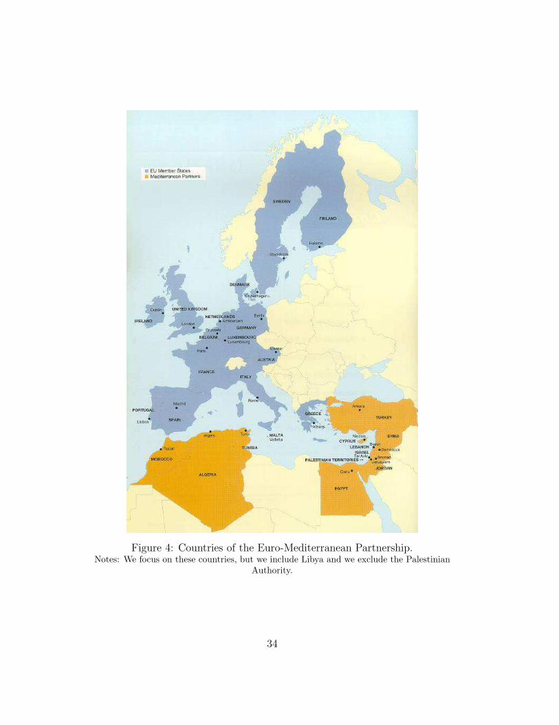
Figure 4: Countries of the Euro-Mediterranean Partnership.Notes: We focus on these countries, but we include Libya and we exclude the Palestinian

Authority.

34

11.

21.

41.

61

1.2

1.4

1.6

11.

21.

41.

61

1.2

1.4

1.6

1970 1980 1990 2000 2010

1970 1980 1990 2000 2010 1970 1980 1990 2000 2010 1970 1980 1990 2000 2010

Austria Belgium Denmark Finland

France Germany Greece Ireland

Italy Luxembourg Netherlands Portugal

United Kingdom Spain Sweden

Pop

ulat

ion

Year

Figure 5: Population trends in the EU countries in 1970-2010.

02

46

80

24

68

02

46

8

1970 1980 1990 2000 1970 1980 1990 2000 1970 1980 1990 2000 1970 1980 1990 2000

Algeria Cyprus Egypt Jordan

Israel Lebanon Libya Malta

Morocco Syria Tunisia Turkey

Population Migration

Year

Figure 6: Population and migration trends in the Third Mediterraneancountries in 1970-2000, normalized to be equal to 1 in 1970.

35