THE CONCEPTUAL BASIS OF

QUANTUM FIELD THEORY

Gerard ’t Hooft

Institute for Theoretical PhysicsUtrecht University, Leuvenlaan 4

3584 CC Utrecht, the Netherlands

and

Spinoza InstitutePostbox 80.195

3508 TD Utrecht, the Netherlands

e-mail: g.thooft@phys.uu.nlinternet: http://www.phys.uu.nl/~thooft/

Published in Handbook of the Philosophy of Science, Elsevier.

December 23, 2004Version 08/06/16

1

Abstract

Relativistic Quantum Field Theory is a mathematical scheme to describethe sub-atomic particles and forces. The basic starting point is that the axiomsof Special Relativity on the one hand and those of Quantum Mechanics on theother, should be combined into one theory. The fundamental ingredients forthis construction are reviewed. A remarkable feature is that the constructionis not perfect; it will not allow us to compute all amplitudes with unlimitedprecision. Yet in practice this theory is more than accurate enough to coverthe entire domain between the atomic scale and the Planck scale, some 20orders of magnitude.

Keywords:

Scalar fields, Spinors, Yang-Mills fields, Gauge transformations, Feynman rules, Brout-Englert-Higgs mechanism, The Standard Model, Renormalization, Asymptotic freedom,Vortices, Magnetic monopoles, Instantons, Confinement.

This version (08/06/16) has some minor typos corrected, and a sign corrected in Eq. (4.8).

Contents

1 Introduction to the notion of quantized fields 3

2 Scalar fields 5

2.1 Classical Theory. Feynman rules . . . . . . . . . . . . . . . . . . . . . . . . 5

2.2 Spontaneous symmetry breaking. Goldstone modes . . . . . . . . . . . . . 9

2.3 Quantization of a classical theory . . . . . . . . . . . . . . . . . . . . . . . 11

2.4 The Feynman path integral . . . . . . . . . . . . . . . . . . . . . . . . . . 13

2.5 Feynman rules for the quantized theory . . . . . . . . . . . . . . . . . . . . 16

3 Spinor fields 20

3.1 The Dirac equation . . . . . . . . . . . . . . . . . . . . . . . . . . . . . . . 20

3.2 Fermi-Dirac statistics . . . . . . . . . . . . . . . . . . . . . . . . . . . . . . 21

3.3 The path integral for anticommuting fields . . . . . . . . . . . . . . . . . . 22

3.4 The Feynman rules for Dirac fields . . . . . . . . . . . . . . . . . . . . . . 24

1

4 Gauge fields 25

4.1 The Yang-Mills equations [3] . . . . . . . . . . . . . . . . . . . . . . . . . . 27

4.2 The need for local gauge-invariance . . . . . . . . . . . . . . . . . . . . . . 29

4.3 Gauge fixing . . . . . . . . . . . . . . . . . . . . . . . . . . . . . . . . . . . 30

4.4 Feynman rules . . . . . . . . . . . . . . . . . . . . . . . . . . . . . . . . . . 33

4.5 BRST symmetry . . . . . . . . . . . . . . . . . . . . . . . . . . . . . . . . 34

5 The Brout-Englert-Higgs mechanism 35

5.1 The SO(3) case . . . . . . . . . . . . . . . . . . . . . . . . . . . . . . . . . 36

5.2 Fixing the gauge . . . . . . . . . . . . . . . . . . . . . . . . . . . . . . . . 37

5.3 Coupling to other fields . . . . . . . . . . . . . . . . . . . . . . . . . . . . . 38

5.4 The Standard Model . . . . . . . . . . . . . . . . . . . . . . . . . . . . . . 39

6 Unitarity 40

6.1 The largest time equation . . . . . . . . . . . . . . . . . . . . . . . . . . . 41

6.2 Dressed propagators . . . . . . . . . . . . . . . . . . . . . . . . . . . . . . 43

6.3 Wave functions for in- and out-going particles . . . . . . . . . . . . . . . . 45

6.4 Dispersion relations . . . . . . . . . . . . . . . . . . . . . . . . . . . . . . . 47

7 Renormalization 47

7.1 Regularization schemes . . . . . . . . . . . . . . . . . . . . . . . . . . . . . 50

7.1.1 Pauli-Villars regularization . . . . . . . . . . . . . . . . . . . . . . . 50

7.1.2 Dimensional regularization . . . . . . . . . . . . . . . . . . . . . . . 51

7.1.3 Equivalence of regularization schemes . . . . . . . . . . . . . . . . . 52

7.2 Renormalization of gauge theories . . . . . . . . . . . . . . . . . . . . . . . 53

8 Anomalies 53

9 Asymptotic freedom 56

9.1 The Renormalization Group . . . . . . . . . . . . . . . . . . . . . . . . . . 56

9.2 An algebra for the beta functions . . . . . . . . . . . . . . . . . . . . . . . 58

10 Topological Twists 59

2

10.1 Vortices . . . . . . . . . . . . . . . . . . . . . . . . . . . . . . . . . . . . . 60

10.2 Magnetic Monopoles . . . . . . . . . . . . . . . . . . . . . . . . . . . . . . 60

10.3 Instantons . . . . . . . . . . . . . . . . . . . . . . . . . . . . . . . . . . . . 61

11 Confinement 63

11.1 The maximally Abelian gauge . . . . . . . . . . . . . . . . . . . . . . . . . 64

12 Outlook 65

12.1 Naturalness . . . . . . . . . . . . . . . . . . . . . . . . . . . . . . . . . . . 65

12.2 Supersymmetry . . . . . . . . . . . . . . . . . . . . . . . . . . . . . . . . . 66

12.3 Resummation of the Perturbation Expansion . . . . . . . . . . . . . . . . . 66

12.4 General Relativity and Superstring Theory . . . . . . . . . . . . . . . . . . 67

1. Introduction to the notion of quantized fields

Quantum Field Theory is one of those cherished scientific achievements that have becomeconsiderably more successful than they should have, if one takes into consideration theapparently shaky logic on which it is based. With awesome accuracy, all known subatomicparticles appear to obey the rules of one example of a quantum field theory that goes underthe uninspiring name of “The Standard Model”. The creators of this model had hardlyanticipated such a success, and one can rightfully ask to what it can be attributed.

We have long been aware of the fact that, in spite of its successes, the Standard Modelcannot be exactly right. Most quantum field theories are not asymptotically free, whichmeans that they cannot be extended to arbitrarily small distance scales. We could easilycure the Standard Model, but this would not improve our understanding at all, becausewe know that, at those extremely tiny distance scales where the problems would becomerelevant, a force appears that we cannot yet describe unambiguously: the gravitationalforce. It would have to be understood first.

Perhaps this is the real strength of Quantum Field Theory: we know where its limitsare, and these limits are far away. The gravitational force acting between two subatomicparticles is tremendously weak. As long as we disregard that, the theory is perfect. And,as I will explain, its internal logic is not shaky at all.

Subatomic particles all live in the domain of physics where spins and actions arecomparable to Planck’s constant h . One obviously needs Quantum Mechanics to describethem. Since the energies available in sub-atomic interactions are comparable to, and oftenlarger than, the rest mass energy mc2 of these particles, they often travel with velocities

3

close to that of light, c , and so relativistic effects will also be important. Thus, in thefirst half of the twentieth century, the question was asked:

“How should one reconcile Quantum Mechanics with Einstein’s theory of Special Rel-ativity?”

As we shall explain, Quantum Field Theory is the answer to this question.

Our first intuitions would be, and indeed were, quite different[1]. One would set upabstract Hilbert spaces of states, each containing fixed or variable numbers of particles.Subsequently, one would postulate a consistent scheme of interactions. What would ‘con-sistent’ mean? In Quantum Mechanics, we have learned how to describe a process wherewe start with a certain number of particles that are all far apart but moving towards oneanother. This is the ‘in’ state |ψ〉in . After the interaction has taken place, we end up withparticles all moving away from one another, a state |ψ′〉out . The probability that a certainin-state evolves into a given out-state is described by a quantum mechanical transitionamplitude, out〈ψ′|ψ〉in . The set of all such amplitudes in the vector spaces formed byall in- and out-states is called the scattering matrix. One can ask how to construct thescattering matrix in such a way that (i) it is invariant under Lorentz transformations,and (ii) obeys the strict laws of quantum causality. By ‘quantum causality’ we mean thatunder no circumstance a measurable effect may proceed with a velocity faster than thatof light. In practice, this means that one must demand that any set of local operatorsOi(x, t) obeys commutation rules such that the commutators [Oi(x, t), Oj(x′, t′)] vanishas soon as the vector (x− x′, t − t′) is space-like. One can show that this implies thatthe scattering matrix must obey dispersion relations.

This is indeed how physicists started to think about their problem. But how shouldone construct such a scattering matrix? Does any systematic procedure exist?

A quantized field may seem to be something altogether different, yet it does appearto allow for the construction of an interacting medium that does obey the laws of Lorentzinvariance and causality. The local operators can be constructed from the fields. All wethen have to do is to set up schemes of relativistically covariant field equations, such asMaxwell’s laws. Even the introduction of non-linear terms in these equations appearsto be straightforward, and if we were to subject such systems to a mathematically well-defined procedure called “quantization”, we would have candidates for a solution to theaforementioned problem.

Realizing that the energy in a quantized field comes in quantized energy packages,which in all respects behave like elementary particles, and, conversely, realizing thatoperators in the form of fields could be defined also when one starts up with Hilbertspaces consisting of elementary particles, it was discovered that quantized fields do indeeddescribe subatomic particles. Subsequently, it was discovered that, in a quantized field,the number of ways in which interactions can be introduced (basically by adding non-linear

4

terms in the field equations), is quite limited. Quantization requires that all interactionscan be given in the form of a Lagrange function L ; relativity requires this L to be Lorentz-invariant, and, most strikingly, self-consistency of Quantum Field Theory then providesfurther restrictions, which leads to the possibility of writing down a complete list of allpossible interactions. The Standard Model is just one element of this list.

The scope of this concise treatise on Quantum Field Theory is too limited to ad-mit detailed descriptions of all technical details. Instead, special emphasis is put on theconceptual issues that arise when addressing the numerous questions and problems asso-ciated with this doctrine. One could use this text to learn Quantum Field Theory, butfor many technical details, more literature must be consulted.[2] We also limited ourselvesto applications of Quantum Field Theory in elementary particle physics. There are manyexamples in low-temperature physics where these and similar techniques are useful, butthey will not be addressed here.

2. Scalar fields

2.1. Classical Theory. Feynman rules

A field is here taken to mean a physical variable that is a function of space-time coordinatesx = (x, t). In order for our theories to be in accordance with special relativity, we willhave to specify how a field transforms under a homogeneous Lorentz transformation,

x′ = Lx . (2.1)

If a field φ transforms as

φ′(x) = φ(x′) , (2.2)

then φ is called a scalar field. The improper Lorentz transformations, such as parityreflection P and time reversal T , are of lesser importance since we know that Nature isnot exactly invariant under those.

Let us first restrict ourselves to real scalar fields; generalization to the case where fieldsare denoted by complex numbers will be straightforward. Upon quantization, scalar fieldswill come in energy packets that behave as spinless Bose-Einstein particles, such as π0, π±

and η0 . Conceptually, the scalar field is the easiest to work with, but in section 9 we shallfind reasons why other kinds of fields can actually improve the internal consistency of ourtheories.

5

Lorentz-invariant field equations typically take the form1

(∂2µ −m2

(i))φi = Fi(φ) ; ∂2µ ≡ ~∂ 2

x − ∂2t . (2.3)

Here, the index i labels different possible species of scalar fields, and Fi(φ) could beany function of the field(s) φj(x). Usually, however, we assume that there is a potentialfunction V int(φ), such that Fi(φ) is the gradient of V int , and furthermore we assumethat V int is a polynomial whose degree is at most four:

V int(φ) = 16gijkφiφjφk + 1

24λijk` φiφjφkφ` ;

Fi(φ) =∂V int(φ)

∂φi= 1

2gijkφjφk + 1

6λijk` φjφkφ` , (2.4)

where g and λ must be totally symmetric under all permutations of their indices.1 Thisis actually a limitation on the forms that Fi(φ) can take. Without this limitation, wewould not have a conserved energy, and quantization of the theory would not be possible.Later, we will see why higher terms in the polynomial are not permitted (section 7).

In order to understand the general structure of the classical solutions to this set ofequations, we temporarily add a function −Ji(x) to Fi(φ) in Eq. (2.3). Multiplying Jitemporarily with a small parameter ε (later to be replaced by 1), we subsequently expandthe solution in powers of ε :

(m2(i) − ∂2

µ)φi(x) = εJi(x)− ∂

∂φiV int(φ(x)) ;

φi(x) = εφ(1)i (x) + ε2φ

(2)i (x) + ε3φ

(3)i (x) + · · ·

=∫

d4y Gij(x− y)(εJj(y)− Fj

(εφ(1)(y) + ε2φ(2)(y) + ε3φ(3)(y) + · · ·

)). (2.5)

The function Gij(x− y) is a solution to the equation

(m2i − ∂2

µ)Gij(x− y) = δijδ(x− y) . (2.6)

Assembling terms of equal order in ε we find a recursive procedure to solve the fieldequations (2.5). At the end of our calculation, we might set ε equal to 1 and Ji(x) equalto zero, or better, have J non-vanishing only in the far-away region where the particlesoriginated, so that the J interaction is a simplified model for the machine that producedthe particles in the far past. Indeed, in the quantum theory it will also turn out to beconvenient to use J as a model for the particle detector at the end of the experiment.

1We use summation convention: repeated indices that are not put between brackets are automaticallysummed over. Greek indices µ are Lorentz indices taking 4 values, Latin indices i, j, · · · run from 1 to 3.Our metric convention is gµν =diag(−1, 1, 1, 1).

6

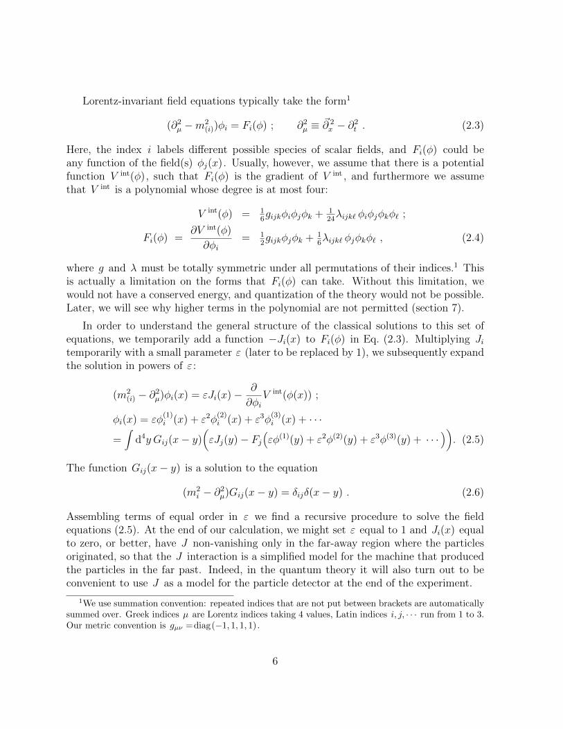
We see that the solution to Eq. (2.5) can be written as the sum of a large number ofterms. Each of these terms can be written in the form of a diagram, called a Feynmandiagram. In these diagrams, we represent a space-time point as a dot, and the functionGij(x− y) as a line connecting x with y . The index i may be indicated at each line. Adot may either be associated with a term Ji(y), or it is a three-point vertex associatedwith a coefficient gijk or a four-point vertex, going with a coefficient λijk` . A typicalFeynman diagram is sketched in Fig. 1.

φ1(x) g

123

λ2456

x′

J4(x′′)

J5(x′′′)

J6(x′ν)

J3(xν)

G33

(x′−xν)

6

5

4

21

Figure 1: Example of a Feynman diagram for classical scalar fields

Observe the general structure of these diagrams. There are factors 12, 1

6, etc., which

can easily be read off from the symmetries of the diagram. By construction, there areno closed loops: the diagram is simply connected. This will be different in the quantizedtheory.

There is one important issue to be addressed: the Green function Gij(x − y) is notcompletely determined by the equation (2.6): one may add arbitrary combinations of thesolutions of the homogeneous equation (m2

i − ∂2µ)Gij(x − y) = 0. In Fourier space, this

ambiguity is reflected in the fact that one has some freedom in choosing the integrationcurve C in the solution2

Gij(x− y) = (2π)−4∫C

d4k eik·(x−y) δijk2 +m2

i

. (2.7)

Our choice can be indicated by shifting the pole by an infinitesimal imaginary number,after which we choose the contour C to be along the real axis of all integrands. Areasonable choice is

G+ij(x− y) = (2π)−4

∫d4k eik·(x−y) δij

k2 − (k0 + iε)2 +m2(i)

, (2.8)

where ε is an infinitesimal, positive number. With this choice, the integration contour inthe complex k0 plane can be shifted such that the imaginary part of k0 can be given an

2An inner product k · x stands for ~k · ~x− k0x0 .

7

arbitrarily large positive value, and from this one deduces that the Green function willvanish as soon as the time difference, x0 − y0 , is negative. This Green function, calledthe forward Green function, gives our expressions the desired causality structure: Thereare obviously no effects that propagate backwards in time, or indeed faster than light.

The converse choice, G−(x−y), gives us the backward solution. However, in the quan-tized theory, we will often be interested in yet another choice, the Feynman propagator,defined as

GFij(x− y) = (2π)−4

∫d4k eik·(x−y) δij

k2 − k02 +m2i − iε

, (2.9)

where, again, the infinitesimal number ε > 0.

The rules to obtain the complete expansion of the solution can now be summarized asfollows:

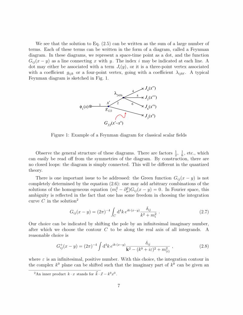
1) Each term can be depicted as a diagram consisting of points (vertices) connected bylines (called propagators). One end-point, , corresponds to a point x wherewe want to know the field φ ; the other end points, , refer to factors J(y(i))for the corresponding points y(i) , see Fig. 1.

2) There are no “closed loops”. i.e. the diagrams must be simply connected (this willbe different in the quantum theory).

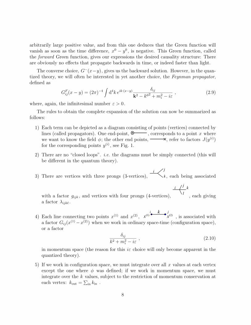
3) There are vertices with three prongs (3-vertices), k

ji

, each being associated

with a factor gijk , and vertices with four prongs (4-vertices),

k

l

ji

, each givinga factor λijk` .

4) Each line connecting two points x(1) and x(2) , x(1) x(2)k ji

, is associated witha factor Gij(x

(1)−x(2)) when we work in ordinary space-time (configuration space),or a factor

δijk2 +m2

i − iε, (2.10)

in momentum space (the reason for this iε choice will only become apparent in thequantized theory).

5) If we work in configuration space, we must integrate over all x values at each vertexexcept the one where φ was defined; if we work in momentum space, we mustintegrate over the k values, subject to the restriction of momentum conservation ateach vertex: kout =

∑in kin .

8

6) A ‘combinatorial factor’. For the classical theories it is 1/N , where N is the numberof permutations of the source vertices that leave the diagram unaltered.

It is not difficult to generalize the rules for the case of higher polynomials in the interac-tions, but this will not be needed for the time being.

2.2. Spontaneous symmetry breaking. Goldstone modes

In the classical theory, the Hamilton density is

H(x, t) = 12φ2i + 1

2(~∂φi)

2 + V (φ) ; V (φ) = 12m2iφ

2i + V int(φ) . (2.11)

The theory is invariant under the group of transformations

φ′i(x) = Aijφj(x) , (2.12)

if A is orthogonal and the potential function V (φ) is invariant under that group. Thesimplest example is the transformation φ↔ −φ :

A = ±1 ; V = V (φ2) = 12a φ2 +

λ

24φ4 . (2.13)

There are two cases to consider:

i) a > 0. In this case, φ = 0 is the absolute minimum of V . We write

a = m2 , (2.14)

and find that m indeed describes the mass of the particle. All Feynman diagramshave an even number of external lines. Since, in the quantum theory, these lines willbe associated with particles, we find that states with an odd number of particlescan never evolve into states with an even number of particles, and vice versa. If wedefine the quantum number PC = (−1)N , where N is the number of φ particles,then we find that PC is conserved during interactions.

ii) a < 0. In this case, we see that:

— trying to identify the mass of the particle using Eq. (2.14) yields the strangeresult that the mass would be purely imaginary. Such objects (“tachyons”)are not known to exist and probably difficult to reconcile with causality, andfurthermore:

— the configuration φ = 0 does not correspond to the lowest energy configura-tion of the system. The lowest energy is achieved when

φ = ±F ; F 2 = −6a/λ . (2.15)

9

It is now convenient to rewrite the potential V as

V =λ

24(φ2 − F 2)2 − C , (2.16)

where we did not bother to write down the value of the constant C , since it doesnot occur in the evolution equations (2.5). There are now two equivalent vacuumstates, the minima of V . Choosing one of them, we introduce a new field variableφ to write

φ ≡ F + φ ;

V =λ

24φ2(2F + φ)2 =

λF 2

6φ2 +

λF

6φ3 +

λ

24φ4 , (2.17)

and we see that

a) for the new field φ , the mass-squared m2 = λF 2/3 is positive, and

b) a three-prong vertex appeared, with associated factor λF . The quantum num-ber PC is no longer apparently conserved.

This phenomenon is called ‘spontaneous symmetry breaking’, and it plays an importantrole in Quantum Field Theory.

Next, let us consider the case of a continuous symmetry. The prototype example is theU(1) symmetry of a complex field. The symmetry group consists of the transformationsA(θ), where θ is an angle:

Φ ≡ 1√2(φ1 + iφ2) ; Φ′ = A(θ)Φ = eiθΦ , (2.18)

Again, the most general potential3 invariant under these transformations is

V (Φ,Φ∗) = aΦ∗Φ + 12λ(Φ∗Φ)2 − C , (2.19)

In the case where the U(1) symmetry is apparent, one can rewrite the Feynman rulesto apply directly to the complex field Φ, noticing that one can write the potential V asa real function of the two independent variables Φ and Φ∗ . With

∂2µΦ =

∂V (Φ,Φ∗)

∂Φ∗, (2.20)

one notices that the Feynman propagators can be written with an arrow in them: anarrow points towards a point x where the function Φ(x) is called for, and away from a

3Observe how we adjusted the combinatorial factors. The choices made here are the most naturalones to keep these coefficients as predictable as possible in future calculations.

10

point x′ where a factor Φ∗(x′) is extracted from the potential V . At every vertex, asmany arrows enter as they leave, and so, during an interaction, the total number of linespointing forward in time minus the number of lines pointing backward is conserved. Thisis an additively conserved quantum number, to be interpreted as a ‘charge’ Q . Accordingto Noether’s theorem, every symmetry is associated to such a conservation law.

However, if a < 0, this U(1) symmetry is spontaneously broken. Then we write

V = 12λ(Φ∗Φ− F 2)2 − C , F 2 ≡ −a/λ . (2.21)

This time, the stable vacuum states form a closed circle in the complex plane of Φ values.Let us write

Φ ≡ F + Φ ; Φ ≡ 1√2(φ1 + iφ2) ;

V = 12λ(F (Φ + Φ∗) + Φ∗Φ

)2

= λF φ21 +

λF√2φ1(φ2

1 + φ22) +

λ

8(φ2

1 + φ22)2 . (2.22)

The striking thing about this potential is that the mass term for the field φ2 is missing.The mass squared for the φ1 field is m2

1 = 2λF . The fact that one of the effective fields ismassless is a fundamental consequence of the fact that we have spontaneous breakdown ofa continuous symmetry. Quite generally, there is a theorem, called the Goldstone theorem:

If a continuous symmetry whose symmetry group has N independent generators, isbroken down spontaneously into a (residual) symmetry whose group has N1 independentgenerators, then N −N1 massless effective fields emerge.

The propagators for massless fields obey Eq. (2.6) without the m2 term, which givesthese expressions an ‘infinite range’: such a Green’s function drops off only slowly for largespatial or timelike separations. These massless oscillating modes are called ‘Goldstonemodes’.

2.3. Quantization of a classical theory

How does one “quantize” a field theory? In the old days of Quantum Mechanics, it wastaught that “you take the Poisson brackets of the classical system, and replace these bycommutators.” Here and there, one had to readjust the order in which classical expressionsemerge, when they are replaced by operators, but the rules appeared to leave no essentialambiguities. Indeed, if such a procedure is possible, one may get a quantum theorywhich reproduces the original classical system in the limit of vanishing h . Also, thegroup of symmetry transformations under which the classical system was invariant, oftenre-emerges in the quantum system.

11

A field theory, however, has a strictly infinite set of physical degrees of freedom (thefield values at every point in 3-space, or, the complete set of Fourier modes). More oftenthan not, upon “quantization”, this leads to infinities that render the theory ill-defined.One has to formulate the notion of “quantization” much more carefully, going throughseveral intermediate steps. Since, today, the answers to our questions are so well known,it is often forgotten how these answers can be derived rigorously and why they take theform they have. What is the strictly logical sequence of arguments?

First of all, it is unreasonable to expect that every classical field theory should havea quantum mechanical counterpart. What we wish to do, is construct some quantumsystem, its Hilbert space and its Hamiltonian, such that in one or more special limits, itreproduces a known classical theory. We demand certain properties of the theory, such asLorentz invariance and causality, but most of all we demand that it be internally logicallyimpeccable, allowing us to calculate how in such a system particles interact, under allimaginable circumstances. We will, however, continue to use the phrase ‘quantization’,meaning that we attempt to construct a quantum theory with a given classical field theoryas its h→ 0 limit.

Often, authors forget to mention the first, very important, step in this logical proce-dure: replace the classical field theory one wishes to quantize by a strictly finite theory.Assuming that physical structures smaller than a certain size will not be important forour considerations, we replace the continuum of three-dimensional space by a discrete butdense lattice of points. In the differential equations, we replace all derivatives ∂/∂xi byfinite ratios of differences: ∆/∆xi , where ∆φ stands for φ(x + ∆x) − φ(x) . In Fourier

space, this means that wave numbers ~k are limited to a finite range (the Brillouin zone),

so that integrations over ~k can never diverge.

If this lattice is sufficiently dense, the solutions we are interested in will hardly dependon the details of this lattice, and so, the classical system will resume Lorentz invarianceand the speed of light will be the practical limit for the velocity of perturbances. Ifnecessary, we can also impose periodic boundary conditions in 3-space, and in that caseour system is completely finite. Finite systems of this sort allow for ‘quantization’ in theold-fashioned sense: replace the Poisson brackets by commutators. Note that we did not(yet) discretize time, so the Hamiltonian of our theory has the form

H = T + V =∑xa

3∏a=1

(∆xa)(

12

∑i

(∂φi/∂t)2 + 1

2

∑i,a

(∆φi∆xa

)2+ V (φ)

). (2.23)

The canonical momenta associated to the fields φi(x) are

pi(x) = (∂φi/∂t)3∏

a=1

(∆xa) , (2.24)

12

and so, we will assume these to be operators obeying:

[φi(x), φj(x′)] = 0 ; [pi(x), pj(x′)] = 0 ; [φi(x), pj(x′)] = iδji δx, x′ . (2.25)

Now, we have to wait and see what happens in the limit of an infinitely dense space-lattice. Will, like the classical theory, our quantum concoction turn out to be Lorentz-invariant? How do we perform Lorentz transformations on physical states? This questionturns out to be far from trivial to answer, but the answer is known. We first need someuseful technical tools.

2.4. The Feynman path integral

The Feynman path integral is often introduced as an “infinite dimensional” integral.Again, we insist on at first keeping everything finite. Label the generalized coordinates(here the φi fields) as qi . The momenta are pi . The Hamiltonian (2.23) is of the conven-tional type (the volume elements

∏ 3a=1(∆xa) act as masses). For future use, we need a

slightly more general one, a Hamiltonian that also contains pieces linear in the momentapi :

H = T + V ; T =∑i

(pi − Ai(q)

)2

2m(i)

; V = V (q) . (2.26)

In principle, we keep the number n of coordinates and momenta finite, in which casethere is no doubt that the differential equations in question have unique, finite solutions(assuming the functions Ai and V to be sufficiently smooth; indeed we will mostly workwith polynomials). Consider the configuration states |q〉 and the momentum states |p〉 .We have

〈q|q′〉 = δn(q− q′) , 〈p|p′〉 = δn(p− p′) ; 〈q|p〉 = (2π)−n/2eipiqi . (2.27)

Taking the order of the operators into account, we write for the kinetic energy

T =∑i

p2i − 2Aipi + A2

i

2m(i)

+ iW (q) ;

W (q) =∑i

[Ai(q), pi]

2im(i)

=∑i

∂iAi(q)

2m(i)

. (2.28)

This enables us to compute swiftly the matrix elements

〈q|H|p〉 = 〈q|p〉(h(q,p) + iW (q)) ; (2.29)

〈p|H|q〉 = 〈p|q〉(h(q,p)− iW (q)) , (2.30)

13

where h(q,p) is the classical Hamiltonian as a function of the two sets of variables q andp .

The evolution operator U(t, δt) for a short time interval δt is

U(t, δt) = e−iH(t)δt = I− iH δt+O(δt)2 . (2.31)

Its matrix elements between states 〈p| and |q〉 are easy to derive now:

〈p|U(t, δt)|q〉 = 〈p|q〉 − iδt〈p|H|q〉+O(δt)2

= (2π)−n/2e−ipiqi(

1− iδth(q,p)− iW (q)+O(δt)2)

= (2π)−n/2 exp(− ip · q− iδth(q,p)− iW (q)+O(δt)2

). (2.32)

What makes this expression very useful is the fact that it does not become singular in thelimit δt ↓ 0. The momentum-momentum and the coordinate-coordinate matrix elementsdo become singular in that limit.

Next, let us consider a finite time interval T . The evolution operator over that timeinterval can formally be viewed as a sequence of many evolution operators over short timeintervals δt , with T = N δt . Using closure, both in p space and in q space, at all timeintervals,

I =∫

dnq |q〉〈q| =∫

dnp |p〉〈p| , (2.33)

we can write

|ψ(qN , T )〉 = 〈qN |U(0, T )|ψ(0)〉 =∫

dnq0

∫dnp0 · · ·

∫dnqN−1

∫dnpN−1

〈qN |pN−1〉 〈pN−1|U(tN−1, δt)|qN−1〉 〈qN−1|pN−2〉〈pN−2|U(tN−2, δt)|qN−2〉 · · · 〈p0|U(0, δt)|q0〉 〈q0|ψ(0)〉 . (2.34)

Plugging in Eq. (2.32), we see that

|ψ(qN , T )〉 =(N−1∏τ=0

∫dnqτ

∫dnpτ

e−W (qτ )δt

(2π)n

)×

exp iN−1∑τ=0

δt(pτ

qτ+1 − qτδt

− h(qτ ,pτ , tτ ))〈q0|ψ(0)〉 . (2.35)

Define

qτ ≡qτ+1 − qτ

δt, (2.36)

14

and

L(p, q, q, t) = p · q− h(q, p, t) , (2.37)

and the measure

N−1∏τ=0

∫dnqτ

∫dnpτ

e−W (qτ )δt

(2π)n≡∫DqDp , (2.38)

then we obtain an expression that seems to be easy to extend to infinitely fine grids inthe time variable:

〈qN |ψ(T )〉 =∫DqDp

(exp i

N−1∑τ=0

δt L(p, q, q, t))〈q0|ψ(0)〉 . (2.39)

In these expressions, we actually allowed the parameters in the Hamiltonian H and theLagrangian L to depend explicitly on time t , so as to expose the physical structure ofthese expressions. Note that

L(p, q, q, t) = −∑i

(pi − Ai −m(i)qi)2

2m(i)

− V (q) +∑i

(Aiqi + 12m(i)q

2i ) , (2.40)

and the integrals over all momentum variables are easy to perform, giving some constantthat only depends on the masses m(i) :

〈qN |ψ(T )〉 =∫Dq exp

(iM−1∑τ=0

δt L(q, q, t))〈q0|ψ(0)〉 , (2.41)

with

L(q, q, t) = T − V ; T =∑i

(12m(i)q

2i + Aiqi) ;

Dq = e−∑

τW (qτ ) δt

N−1∏τ=0

(dnqτ

∏i

( m(i)

2π δt

) 12

). (2.42)

Actually, L(q, q, t) is obtained from L(p,q, q, t) by extremizing the latter with respectto p :

∂

∂piL(p,q, q, t) = 0 ; qi =

∂h(q,p, t)

∂pi. (2.43)

This is exactly the standard relation between Lagrangian and Hamiltonian of the classicaltheory. So, L is indeed the Lagrangian.

15

If the continuum limit exists, the exponent in Eq. (2.41) is exactly i times the classicalaction,

S =∫

dtL(q, q, t) . (2.44)

It is tempting to assume that the O(δt)2 terms in Eq. (2.31) disappear in the limit; afterall, they are only multiplied by factors N ≈ C/δt . In that case, the evolution operator inEq. (2.41) clearly takes the form of an integral over all paths going from q0 to qN . Thisis Feynman’s path integral. In the case of a field theory, one considers the field definedon a lattice in space, and since the path integral starts with a lattice in the time variable,we end up dealing with a lattice in space and time. In conclusion:

The evolution operator in a field theory is described by first rephrasing thetheory on a dense lattice in space-time. Replacing partial derivatives by thecorresponding finite difference ratios, one writes an expression for the actionS of the theory. Normally, it can be written as an integral over a Lagrangedensity, L(φ, ∂µφ). The evolution operator of the theory is obtained by in-tegrating eiS over all field configurations φ(x, t) in a given space-time patch.The integration measure is defined from Eq. (2.42).

The Ai terms, linear in the time derivatives, do not play a role in scalar field theories butthey do in vector theories, and the fact that they occur in the measure (2.42) is usuallyignored. Indeed, in most cases, W (q) vanishes, but we must be aware that it might causeproblems in some special cases. We ignore the W term for the time being.

2.5. Feynman rules for the quantized theory

The Feynman rules for quantized field theories were first derived by careful analysis ofperturbation theory. Writing the quantum Hamiltonian H as H = H0 + H int , oneassembles all terms bilinear in the fields and their derivatives in H0 and performs theperturbation expansion for small values of H int . This leads to a set of calculation rulesvery similar to the rules derived for a classical theory, see subsection 2.1. Most of theserules (but not everything) can now most elegantly be derived from the path integral.

Let us first derive these rules for computing a finite dimensional integral of the type(2.41). Although often our action will not contain terms linear in the variables qi(t), wedo need such terms now, so, if necessary, we add them by hand, only to remove them atthe end of the calculations. There is no need to indicate the time variable t explicitly; weabsorb it in the indices i . the action is then

S(q) =∑x,t

L(x, t) = Jiqi − 12Mijqiqj − 1

6Aijkqiqjqk − 1

24Bijk`qiqjqkq` . (2.45)

16

To calculate∫

dNq eiS(q) , we keep only the bilinear part (the term with the coefficientsMij ) inside the exponent, and expand the exponent of all other terms:

out〈0|0〉in = C∫

dNq(

exp(− 1

2iMijqiqj

)) ∞∑k=0

∞∑`=0

∞∑m=0

1

k!`!m!×

(iJi1qi1) · · · (iJikqik) (− i6Ai1j1k1 qi1qj1qk1) · · · (− i

6Ai j`k` qi qj`qk`)

(− i24Bi1j1k1`1

qi1qj1qk1q`1) · · · (− i24Bimjmkm`m

qimqjmqkmq`m) . (2.46)

(C is a constant not depending on the coefficients, but only on their dimensionality).

We can calculate all of these integrals if we know how to do the J terms. Thesehowever can be done to all orders since we know exactly how to do the Gaussian integral∫

dNq exp i(−12Mijqiqj + Jiqi) =

(2π)N2

(det(M))12

exp(

12iJiM

−1ij Jj

)=

C∞∑k=0

1

k!

(12iJi1M

−1i1j1

Jj1

)· · ·

(12iJikM

−1ikjk

Jjk

). (2.47)

This expression tells us how to do the integrals in Eq. (2.46) by collecting terms that gowith given powers of Ji . The outcome of this calculation can be summarized in a conciseway:

1) Each term can be depicted as a diagram consisting of points (vertices) connected bylines (propagators). The lines may end at points i , , which refer to factorsJi .

2) There are vertices with three prongs (3-vertices), k

ji

, each being associated

with a factor Aijk , and vertices with four prongs (4-vertices),

k

l

ji

, each givinga factor Bijk` .

3) Each line connecting two points i and j , is associated with a factor M−1ij .

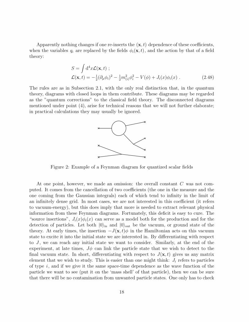
4) In contrast with the classical theory, however, the diagrams may contain discon-nected pieces, or multiply connected parts: closed loops. See Fig. 2.

5) There are combinatorial factors arising from the coefficients such as k! in Eq. (2.46).One can gain experience in deriving these factors; they follow directly from thesymmetry structure of a diagram. This technical detail will not be further addressedhere.

17

Apparently nothing changes if one re-inserts the (x, t) dependence of these coefficients,when the variables qi are replaced by the fields φi(x, t), and the action by that of a fieldtheory:

S =∫

d4xL(x, t) ;

L(x, t) = −12(∂µφi)

2 − 12m2

(i)φ2i − V (φ) + Ji(x)φi(x) . (2.48)

The rules are as in Subsection 2.1, with the only real distinction that, in the quantumtheory, diagrams with closed loops in them contribute. These diagrams may be regardedas the ”quantum corrections” to the classical field theory. The disconnected diagramsmentioned under point (4), arise for technical reasons that we will not further elaborate;in practical calculations they may usually be ignored.

Figure 2: Example of a Feynman diagram for quantized scalar fields

At one point, however, we made an omission: the overall constant C was not com-puted. It comes from the cancellation of two coefficients (the one in the measure and theone coming from the Gaussian integrals) each of which tend to infinity in the limit ofan infinitely dense grid. In most cases, we are not interested in this coefficient (it refersto vacuum-energy), but this does imply that more is needed to extract relevant physicalinformation from these Feynman diagrams. Fortunately, this deficit is easy to cure. The“source insertions”, Ji(x)φi(x) can serve as a model both for the production and for thedetection of particles. Let both |0〉in and |0〉out be the vacuum, or ground state of thetheory. At early times, the insertion −J(x, t)φ in the Hamiltonian acts on this vacuumstate to excite it into the initial state we are interested in. By differentiating with respectto J , we can reach any initial state we want to consider. Similarly, at the end of theexperiment, at late times, Jφ can link the particle state that we wish to detect to thefinal vacuum state. In short, differentiating with respect to J(x, t) gives us any matrixelement that we wish to study. This is easier than one might think: Ji refers to particlesof type i , and if we give it the same space-time dependence as the wave function of theparticle we want to see (put it on the ‘mass shell’ of that particle), then we can be surethat there will be no contamination from unwanted particle states. One only has to check

18

the normalization, but also that is not hard: we adjust the 1-particle to 1-particle ampli-tude to be one; a single particle cannot scatter (it could be unstable, but that is anothermatter). The constant C always drops out of these calculations.

An important point is the ambiguity of the inverse matrix M−1 . As in the classicalcase, there are homogeneous solutions, so, if we work in momentum space, there will bethe question how to integrate around the poles of the propagator. The iε prescriptionmentioned in subsection 2.1 is now imperative. This is explained as follows. Consider thepropagator in position space, and choose its poles situated as follows:∫

d4keik·x−ik

0t

m2 + k2 − k02 − iε; ε ↓ 0 . (2.49)

The poles are at k0 = ±(√m2 + k2 − iε). Now consider this propagator at time t =

−T + iβ with both T and β large. Since β is large, the choice of the contour at negativek0 is immaterial, since the exponential there is very small. At positive k0 , we choose thecontour to go above the pole, so the imaginary part of k0 is chosen positive. We see thatthen the exponential vanishes rapidly at negative time. In short, our propagator tends tozero if the time t tends to −T + iβ when both T and β are large and positive. The sameholds for t→ +T − iβ . Indeed, we want our evolution operator to be dominated by theempty diagram in these two limits. Write:

〈ψ|U(0, +T − iβ)|ψ′〉 =∑E

〈ψ|E〉 exp(−iET − βE) 〈E|ψ′〉 , (2.50)

where |E〉 are the energy eigenstates. At large β , the vacuum state should dominate.Conversely, if we consider evolution backwards in time, the other iε prescription is needed.One then works with the Feynman rules for the inverse, or the complex conjugate, of thescattering matrix.

Now, we are in a position to add the prescription how to identify the external lines(the lines sticking out of the diagram) with in- and out-going particles. For an ingoingparticle, we use a source function J(x) whose Fourier components emit a positive amountof energy k0 . For an out-going particle the source emits a negative k0 . According tothe rules formulated above, these sources would be connected to the rest of the diagramby propagators, in Fourier space (k2

µ +m2 − iε)−1 . Since the in- and out-going particleshave k2

µ +m2 = 0 , we must take the residue of the pole. In practice, this means that wehave to remove the external propagators, a procedure called ‘amputation’. One then stillhas to establish a normalization factor. This factor is most easily obtained by checkingunitarity of the scattering matrix, using the optical theorem. At first sight, this seemsto be just a simple numerical coefficient, but there is a slight complication at higherorders, when self-energy corrections affect the propagator. These corrections also removeunstable particles from the physical scattering matrix. We return to this in Section 6.The complete Feynman rules are listed in subsection 4.4

19

3. Spinor fields

3.1. The Dirac equation

The fields introduced in the previous section can only be used to describe particles withspin 0. In a quantum theory, particles can come in any representation of the little group,which is the subgroup of the inhomogeneous Lorentz group that leaves the 4-momentumof a particle unaffected. For massive particles in ordinary space, this is the group ofrotations of a three-vector, SO(3). Its representations are labelled by either an integer≥ 0, or an integer +1

2, representing the total spin of a particle. So, next in line are

the particles with spin 12. The wave function for such a particle has two components,

one for spin up and one for spin down. Therefore, to describe a relativistic theory withsuch particles, we should use a two-component field obeying a relativistically covariantfield equation. Paul Dirac was the first to find an appropriate relativistically covariantequation for a free particle with spin 1

2:

(m+∑µ

γµ∂µ)ψ(x) = 0 , (3.1)

but the field ψ(x, t) has four complex components. Here, γµ, µ = 0, 1, 2, 3, are four 4×4matrices, obeying

γµ, γν = γµγν + γνγµ = 2gµν ; ㆵ = gµνγν . (3.2)

In contrast to the scalar case, the Dirac equation is first order in the space- and time-derivatives, and furthermore, one could impose a ‘reality condition’ (Majorana condition)on the fields, of the form

ψ(x) = Cψ∗(x) , γµC = C(γµ)∗ , µ = 0, 1, 2, 3. (3.3)

These two features combined give the Dirac field the same multiplicity as two scalar fields.Usually, we do not impose the Majorana condition, so that the Dirac field is truly complex,having a conserved U(1) charge much like a complex scalar field.

We briefly recapitulate the most salient features of the Dirac equation. The 4 × 4Dirac matrices can conveniently be expressed in terms of two commuting sets of Paulimatrices, σa and τa . Define

σ1 =(

0 11 0

), σ2 =

(0 −ii 0

), σ3 =

(1 00 −1

), (3.4)

and similarly for the τ matrices, except that they act in different spaces: a Dirac index isthen viewed as a pair (iα) of indices i and α , such that the matrices σa act on the firstindex i , and the matrices τA act on the indices α . We have:

σaσb = δab + iεabcσc , τAτB = δAB + iεABCτC , [σa, τB] = 0 . (3.5)

20

Define (with the convention gµν =diag(−1, 1, 1, 1))

γ1 = σ1τ1 , γ2 = σ2τ1 , γ3 = σ3τ1 , γ0 = −iτ3 . (3.6)

The matrix C in Eq. (3.3) is then:

C = γ2γ4 . (3.7)

In the non-relativistic limit, the Dirac equation reads

(m+ iγµkµ)ψ ≈ (m− iγ0k0)ψ ≈ m(1− τ3)ψ = 0 , (3.8)

so that only two of the four field components survive (the ones with τ3|ψ〉 = |ψ〉 ).

3.2. Fermi-Dirac statistics

At this point, we could now attempt to pursue our fundamental quantization program:produce the Poisson brackets of the system, replace these by commutators, rewrite theHamiltonian of the system in operator form, and solve the resulting Schrodinger equation.

Unfortunately, if one uses ordinary (commuting) numbers, this does not work. TheLagrangian associated to the Dirac equation will read

L =∫

d3~xL(x) ; L(x) = −ψ(x)(m+4∑

µ=0

γµ∂µ)ψ(x) , (3.9)

and the canonical procedure would give as momentum fields:

pψ(~x) =∂L

∂(∂0ψ(~x))= ψ(~x)γ0 , pψ(~x) = 0 . (3.10)

From this, one finds the Hamiltonian:

H =∫

d3~xH(~x) ; H(~x) = pψ ψ − L(~x) = ψ(x)(m+3∑i=1

γi∂i)ψ(x) , (3.11)

Here, the index i is a spatial one, runnunig from 1 to 3. This, however, is not boundedfrom below! Such a quantum theory would not possess a vacuum state, and hence beunsuitable as a model for Nature.

For a better understanding of the situation, we strip the Dirac equation to its barebones. After diagonalizing it, we find that the Lagrangian consists of elementary units ofthe form

L = ψ(i∂tψ −Mψ) ; pψ = iψ ; H = ψMψ . (3.12)

21

If we were using ordinary numbers, the only way to obtain a lower bound on H wouldbe by identifying ψ with ψ . Then, however, the kinetic part of the Lagrangian wouldbecome a time-derivative:

ψ∂tψ → 12∂t(ψ ψ) , (3.13)

so that it could not contribute to the action. One concludes that, only in the space ofanticommuting numbers, can the Lagrangian (3.12) make sense. Thus, one replaces thePoisson brackets for ψ and ψ by anticommutators:

ψ, ψ ≡ ψ ψ + ψ ψ = 1 ; ψ, ψ = 0 ; ψ, ψ = 0 . (3.14)

The elementary representation of this algebra is in a ‘Hilbert space’ consisting of just twostates (the empty state and the one-particle state), in which the operators ψ and ψ actas annihilators and creators:

ψ =(

0 10 0

); ψ =

(0 01 0

); H =

(0 00 M

). (3.15)

Returning to the non-diagonalized case, we can keep the Lagrangian (3.9) and Hamiltonian(3.11) when the anticommutation rules (3.14) are replaced by

ψi(x), ψj(x′) = δij δ(x− x′) ;

ψi(x), ψj(x′) = 0 ; ψi(x), ψ

j(x′) = 0 . (3.16)

The anticommutation rules (3.16) turn Dirac particles into fermions. It appears to be acondition for any Lorentz-invariant quantum theory to be consistent, that integer spinparticles must be bosons and particles whose spin is an integer +1

2must be fermions.

3.3. The path integral for anticommuting fields

Let us now extend the notion of path integrals to include Dirac fields. This means wehave to integrate over anticommuting numbers, to be called θi , where i is some index(possibly including x). They are numbers, not operators, so all anticommutators vanish.Consider the Taylor expansion of a function of a variable θ . Since θ2 = 0, this expansionhas only two coefficients:

f(θ) = f(0) + f ′(0)θ . (3.17)

So, this is the most general function of θ that one can have. It is generally agreed thatone should define integrals for anticommuting numbers θ by postulating∫

dθ 1 ≡ 0 ;∫

dθ θ ≡ 1 . (3.18)

22

The reason for this definition is that one can manipulate these expressions in the sameway as integrals over ordinary numbers:∫

dθ f(θ + α) =∫

dθ f(θ) ;∫

dθ∂f(θ)

∂θ= 0 , (3.19)

etc.

Now, consider the Hamiltonian for just one fermionic degree of freedom, (3.15), whichwe write as

H = M b†b ; b, b† = 1 ; b2 = (b†)2 = 0 , (3.20)

and a wave function ψ =(ψ0

ψ1

). Define the following function of θ :

ψ(θ) ≡ ψ0θ + ψ1 , (3.21)

This now serves as our wave function. It is not hard to derive how the annihilationoperator b and the creation operator b† act on these wave functions:

if φ = b ψ then φ(θ) = θ ψ(θ) , (3.22)

or:

b = θ ; b† =∂

∂θ. (3.23)

We now wish to express the evolution of a fermionic wave function in terms of a pathintegral, just as in subsection 2.4. Consider a short time interval δt . Then, ignoring allterms of order (δt)2 , one derives

e−iδtHψ(θ1) = ψ0 θ1 + (1− iM δt)ψ1

=∫

dθ0(−θ1 + θ0 − iMδtθ0)(ψ0θ0 + ψ1)

=∫

dθ0

∫dθ(1 + θ(−θ1 + θ0 − iMδtθ0)

)ψ(θ0)

=∫

dθ0

∫dθ eθ(−θ1+θ0−iMδtθ0)ψ(θ0) . (3.24)

Repeating this procedure over many infinitesimal time intervals, with T = N δt , onearrives at the formal expression

ψ(θT ) =∫

dθT−1dθT−1 · · · dθ0dθ0 expN−1∑τ=0

δt(θτ (−θτ+1 + θτ

δt− iMθτ )

)ψ(θ0) . (3.25)

23

The exponential tends to

i∫

dt L(t) . (3.26)

Thus, as in the bosonic case, the evolution operator is formally the path integral of eiS

over all (anticommuting) fields ψi(x, t), where the action S is the time integral4. of theLagrangian L , and indeed the space-time integral of the Lagrange density L(x, t).

3.4. The Feynman rules for Dirac fields

Let Mij be any matrix that can be diagonalized. Using Eqs. (3.18), we find the integral

∏i

∫dθi

∫dθi e

θiMijθj = detij

(M) , (3.27)

which can be easily checked by diagonalizing M , and writing∫dθ∫

dθ eθMθ =∫

dθ∫

dθ (1 + θMθ) = M . (3.28)

Thus, a Gaussian integral over anticommuting numbers gives a result very similar to thatover commuting numbers, except that we get det(M) rather than C/ det(M). Writing

M = M0 + δM ;

det(M) = eTr(logM)) = 1 + Tr (logM) + 12(Tr logM)2 + · · · , (3.29)

we see that this can be obtained from det(M−1) by switching the signs of all odd termsin this expansion. Since the N th term corresponds to a Feynman diagram with N closedfermionic loops, one derives that the Feynman rules can be read off from the ones forordinary commuting fields, by switching a sign whenever a closed fermionic loop is en-countered.

We have

−Tr logM = −Tr logM0 +∞∑n=1

(−1)n

nTr (M−1

0 δM)n . (3.30)

Here, as in the bosonic case, −M0 is the propagator of the theory, and δM representsthe contribution from any perturbation. Thus, if our Lagrangian, including possibleinteraction terms, is

L = −ψi(m(i) + γµ∂µ)ψi + ψigij(φ)ψj , (3.31)

4In some applications, careful considerations of the boundary conditions for Dirac’s equation, requirean extra boundary term to be added to the action (3.25)

24

then the propagator, in Fourier space, is

(m(i) + iγµkµ)−1 =m(i) − iγµkµm2

(i) + k2 − iε, (3.32)

while gij(φ) generates the interaction vertices of a Feynman diagram. The iε term ischosen as in bosonic theories, for the same reason as there: the vacuum state must be thestate with lowest energy.

The poles in the propagator can be used to define in- and out-going particles, byadding source terms to the Lagrangian:

δL = η(x)ψ + ψη(x) , (3.33)

where η(x) and η(x) are kept fixed, as anticommuting numbers. We could proceed toderive the precise rules for in- and out-going particles with spin up or down, but it ismore convenient to postpone this until we discuss the unitarity property of the S -matrix,where these rules are required explicitly, and where we find the precise prescription forthe normalization of these states (section 6).

Note that our Lagrangian is always kept to be bilinear in the anticommuting fields.This is because we insist that L itself must be a commuting number and, furthermore,terms that are quartic in the fermionic fields have too high a dimension. We will see insection 7 why such terms have to be avoided.

4. Gauge fields

We continue to search for elementary fields, whose Lorentz covariant field equations can besubject to our quantization program. In principle, such fields could come as any arbitraryrepresentation of the Poincare algebra, that is, we might consider any kind of tensor field,Aµνλ···(x, t). It turns out, however, that tensors with more than one Lorentz index cannotbe used. This is because we wish the energy density of a field to be bounded from below,and in addition, we wish the dimensionality of the interactions to be sufficiently low, suchthat all coupling strengths have mass dimension zero or positive.

A theory is called “renormalizable” if all of its interaction parameters λi (that is,all parameters with respect to which we need to make a perturbation expansion) have amass-dimensionality that is positive or zero. In practice, the dimensionality of couplingcoefficients is easy to establish: in n space-time dimensions, all terms in the LagrangianL have dimensionality [mass]n . The mass-dimensionality of all fields and parameters canthen be read off: dim(λ) = [m]4−n , dim(λ3) = [m]3−n/2 , etc.

Coupling strengths with mass dimension less than zero give rise to unacceptably diver-gent expressions for the contributions of the interactions at short scales. A prime example

25

of a field one would like to include is the gravitational field described by the metric gµν(x),but its only possible interaction is the gravitational one, whose coupling strength, New-ton’s constant GN , has the wrong dimension. The non-renormalizable theories one thenobtains are the subject of intense investigations but fall outside the scope of this paper(see C. Rovelli’s contribution in this book).

So, only spin-one fields Aaµ(x) are left for consideration. Here, µ is a Lorentz index,while the number of field types is counted by the index a = 1, · · · , NV . These fields shoulddescribe the creation and annihilation of spin-one particles. When at rest, such a particlewill be in one of three possible spin states. Yet, to be Lorentz-invariant, a vector field Aµshould have four components. One of these, at least, should be unphysical, although onemight think of accepting an extra, spinless particle to be associated to the vector particles.More important therefore is the consideration that, in the corresponding classical theory,the energy should be bounded from below.

This then rules out the treatment of a four-vector field as if we had four scalar fields,because the Lorentz-invariant product has an indefinite metric. Can we construct a La-grangian for a vector field that gives a Hamiltonian that is bounded from below?

Let us look at the high-momentum limit for one of these vector fields. The only twoterms in a Lagrangian that can survive there are:

L = −12α (∂µAν)

2 + 12β ∂µAµ ∂νAν , (4.1)

since other terms of this dimensionality can be reduced to these ones by partial integrationof the action, while mass terms (terms without partial derivatives) become insignificant.We have for the canonical momentum fields

Ei =∂L∂∂0Ai

= α ∂0Ai (i = 1, 2, 3);

E0 =∂L

∂∂0A0

= (β − α) ∂0A0 − β ∂iAi . (4.2)

Now, consider the Hamiltonian density H = Eµ ∂0Aµ − L . It must be bounded frombelow for all field configurations Aµ(x, t). Let us first consider the case when the spacelikecomponents Ai and all spacelike derivatives ∂i are negligible compared to ∂0A0 :

H → 12(β − α)(∂0A0)2 , (4.3)

then, when A0 and all time-derivatives are negligible:

H → 12α(∂iAj)

2 − 12β(∂iAi)

2 . (4.4)

These must all be bounded from below. Eq. (4.3) dictates that β ≥ α , while Eq. (4.4)dictates that α ≥ β . We conclude that α = β , which we can both normalize to one.

26

Since total derivatives in the Lagrangian do not count, we can then rewrite the originalLagrangian (4.1) as

L → −14F aµνF

aµν , F a

µν = ∂µAaν − ∂νAaµ . (4.5)

Realizing that this is the Lagrangian for ordinary QED, we know that its energy-densityis properly bounded from below. We conclude that every vector field theory must have aLagrangian that approaches Eq. (4.5) at high energies and momenta.

We do note, that with the choice α = β , both (4.3) and (4.4) tend to zero. Indeed,any field Aaµ that can be written as a space-time gradient, Aaµ = ∂µΛa(x, t), has F a

µν = 0,and hence contributes neither to the Lagrangian nor to the Hamiltonian. Such fields couldbe arbitrarily strong, yet carry zero energy. They would represent particles and forceswithout energy. This is unacceptable in a decent Quantum Field Theory. How do weprotect our theory against such features?

There is exactly one way to do this. We must make sure that field replacements ofthe type

Aaµ → Aaµ + ∂µΛa(x) + · · · , (4.6)

do not affect at all the physical state that we are describing. This is what we call alocal gauge transformation. We must insist that our theory is invariant under local gaugetransformations. The ellipses in Eq. (4.6) indicate that we allow extra terms that do notcontribute to the bilinear part of the Lagrangian (4.5). Thus, we arrive at Yang-Millsfield theory.

4.1. The Yang-Mills equations [3]

Our conclusion from the above is that every vector field is associated to a local gaugesymmetry. The dimensionality of the local gauge group must be equal to NV , the numberof vector fields present. Besides the vector fields, the local symmetry transformations mayalso affect the scalar and spinor fields. In short, the vector fields must be Yang-Mills fields.We here give a brief summary of Yang-Mills theory.

We have a local Lie group with elements Ω(x) at the point x . Let the matricesT a, a = 1, · · · , NV be its infinitesimal generators:

Ω(x) = I + i∑a

Λa(x)T a ; T a = (T a)† . (4.7)

Characteristic for the group are its structure constants fabc :

[T a, T b] = −ifabcT c . (4.8)

27

As is well-known in group theory, one can choose the normalization of T a in such a waythat the fabc are totally antisymmetric:

fabc = −fbac = fbca . (4.9)

Usually, the spinor fields ψ(x) and scalar fields φ(x) are introduced in such a way thatthey transform as (sets of irreducible) representations of the gauge group. A local gaugetransformation is then:

ψ′(x) = Ω(x)ψ(x) ; φ′(x) = Ω(x)φ(x) , (4.10)

and in infinitesimal form:

ψ′(x) = ψ(x) + iΛa(x)T aψ(x) +O(Λ)2 , (4.11)

and similarly for φ(x). The dimension of the irreducible representation can be differentfor different field types. So, scalar and spinor fields usually form gauge-vectors of variousdimensionalities. In these, and in the subsequent expressions, the indices labelling thevarious components of the fields ψ , Ω and T a have been suppressed.

Our vector fields Aaµ(x) are most conveniently introduced by demanding the possibilityof constructing gauge-covariant gradients of these fields:

Dµψ(x) ≡ (∂µ + igAaµ(x)T a)ψ(x) , (4.12)

where g is a freely adjustable coupling parameter. The repeated indices a , denoting thedifferent species of vector fields, are to be summed over. By demanding the transformationrule

(Dµψ(x))′ = Ω(x)Dµψ(x) = Dµψ(x) + iΛa(x)T aDµψ(x) +O(Λ)2 , (4.13)

one easily derives the transformation rule for the vector fields Aaµ(x):

igAaµ′(x)T a = Ω(x)

(∂µ + igAaµ(x)T a

)Ω−1(x)

= igAaµ(x)T a − i∂µΛa(x)T a + g[T a, T b]Λa(x)Abµ(x) (4.14)

(omitting the O(Λ)2 terms). With Eq. (4.8), this becomes

Aaµ′(x) = Aaµ(x)− 1

g∂µΛa(x) + fabcΛ

b(x)Acµ(x) . (4.15)

If we ensure that all gradients used are covariant gradients, we can directly constructthe general expressions for Lagrangians for scalar and spinor fields that are locally gauge-invariant:

Linvscalar(x) = −1

2(Dµφ)2 − V (φ2) ; (4.16)

LinvDirac(x) = −ψ(γµDµ +m)ψ , (4.17)

28

and in addition other possible invariant local interaction terms without derivatives.

The commutator of two covariant derivatives is

[Dµ, Dν ]ψ(x) = igF aµν(x)T aψ(x) ;

F aµν(x) = ∂µA

aν − ∂νAaµ + gfabcA

bµA

cν . (4.18)

Unlike Aaµ(x) or the direct gradients of Aaµ(x), this Yang-Mills field F aµν transforms as a

true adjoint representation of the local gauge group:

F aµν′(x) = F a

µν(x) + fabcΛb(x)F c

µν(x) . (4.19)

This allows us to construct a locally gauge invariant Lagrangian for the vector field:

LinvYM(x) = −1

4F aµν(x)F a

µν(x) . (4.20)

The structure constants fabc in the definition 4.18 of the field F µν implies the presenceof interaction terms in the Yang-Mills Lagrangian 4.20. If fabc is non-vanishing, we talkof a non-Abelian gauge theory.

There is one important complication in the case of fermions: the Dirac matrix γ5 ≡γ1γ2γ3γ4 can be used to project out the chiral sectors :

ψ ≡ ψL + ψR ; ψL = 12(1 + γ5)ψ ; ψR = 1

2(1− γ5)ψ . (4.21)

Since the kinetic part of a Dirac Lagrangian can be split according to

LDirac = −ψL(γD)ψL − ψR(γD)ψR , (4.22)

we may choose the left-handed fields ψL to be in representations different from the right-handed ones, ψR . However, since a mass term joins left to right:

−mψψ = −mψLψR −mψRψL , (4.23)

such terms would then be forbidden, hence such chiral fields must be massless. Secondly,not all combinations of chiral fermions are allowed. An important restriction is discussedin section 8. The fields ψL turn out to describe spin- 1

2massless particles with only the left-

rotating helicity, while their antiparticles, described by ψL , have only the right-rotatinghelicity.

4.2. The need for local gauge-invariance

In the early days of Gauge Theory, it was thought that local gauge-invariance could bean ‘approximate’ symmetry. Perhaps one could add mass terms for the vector field that

29

violate local symmetry, but make the model look more like the observed situation in par-ticle physics. We now know, however, that such models suffer from a serious defect: theyare non-renormalizable. The reason is that renormalizability requires our theory to beconsistent up to the very tiniest distance scales. A mass term would, at least in principle,turn the field configurations described by the Λ(x) contributions in Eq. (4.15) into physi-cally observable fields (the Lagrangian now does depend on Λ(x)). But, since the kineticterm for Λ(x) is lacking, violently oscillating Λ fields carry no sizeable amount of energy,so they would not be properly suppressed by energy conservation. Uncontrolled shortdistance oscillations are the real, physical cause for a theory being non-renormalizable.

It is similar uncontrolled short-distance fluctuations of the space-time metric that causethe quantized version of General Relativity (“Quantum Gravity”) to be non-renormal-izable. Drastic measures (String Theory?) are needed to repair such a theory.

Since renormalizability provides the required coherence of our theories, local gaugesymmetry, described by Eqs. (4.10) and (4.15), must be an exact, not an approximatesymmetry of any Quantum Field Theory.5 Obviously, the fact that most vector particlesin the sub-atomic world do carry mass must be explained in some other way. It is herethat the Brout-Englert-Higgs mechanism comes to the rescue, see Section 5.

4.3. Gauge fixing

The longitudinal parts of the vector fields do not occur directly in the Yang-Mills La-grangian (4.20), exactly because of its invariance under transformations of the form (4.15).Yet if we wish to describe solutions, we need to choose a longitudinal component. Thisis why we wish to impose some additional constraint, the so-called gauge condition, onour description of the solutions, both in the classical and in the quantized theory. Inelectrodynamics, we usually impose a constraint such as ∂µAµ(x) = 0 or A0 = 0. In aYang-Mills theory, such a constraint is needed for each value of the index a . A gaugefixing term is indicated by a field Ca(x) which is put equal to zero:

Ca(x) = 0 ; a = 1, · · · , NV ; where (4.24)

either Ca(x) = ∂µAaµ(x) (Feynman gauge), (4.25)

or Ca(x) = Aa0(x) (timelike gauge), (4.26)

or other possible gauge choices. It is always possible to find a Λa(x) that obeys such acondition. For instance, to obtain the Feynman gauge (4.25), all one has to do is extremizean integral under variations of the gauge group:

δ∫

d4x(Aaµ(x)

)2=∫

d4x 2AµDµΛ = 0 → DµAµ(x) = ∂µAaµ(x) = 0 . (4.27)

5One apparent exception could be the case where the longitudinal component decouples completely,which happens in massive QED. But even in that case, it is better to view the longitudinal photon as aHiggs field, see section 5.

30

For the classical theory, the most elegant way to impose such a gauge condition is byadding a Lagrange multiplier term to the Lagrangian:

L(x) = Linv(x) + λa(x)Ca(x) , (4.28)

where Ca(x) is any of the possible gauge fixing terms and λa(x) a free kinematical vari-able. Here, Linv stands for the collection of all gauge-invariant terms in the Lagrangian.The Euler-Lagrange equations of the theory then automatically yield the Yang-Mills fieldequations plus the constraint, apart from a minor detail: the boundary condition. Varyingthe gauge transformations, one finds, since Linv does not vary, Dµλ

a(x) = 0. We need toimpose the stricter equation λa(x) = 0, which is obtained by imposing λa(x) = 0 at theboundaries of our system.

Alternatively, one can replace the invariant Lagrangian by

L(x) = Linv(x)− 12

(Ca(x)

)2, (4.29)

which has the advantage that, after partial integration, the bilinear part becomes verysimple: L = −1

4FµνFµν − 1

2(∂µA

µ)2 → −12(∂µAν)

2 , so that the vector field can be treatedas if it were just 4 scalars. Again, varying the gauge transformation Λa(x), one findsDµC

a(x) = 0, which must be replaced by the more stringent condition Ca(x) = 0 byadding the appropriate boundary condition.

Note that the Lagrange-Hamilton formalism could give the wrong sign to the energy ofsome field components; we should continue to use the energy deduced before imposing thegauge constraint. If we use the timelike gauge (4.26), the energy is correct, but the theoryappears to lack Lorentz invariance. Lorentz transformations must now be accompaniedby gauge transformations.

How is the gauge constraint to be handled in the quantized theory? This problem wassolved by B.S. DeWitt[4],[5] and by Faddeev and Popov[6]. The gauge constraint is to beimposed in the integrand of the functional integral:

Z =∫DA(x)

∫Dφ(x) · · · ei

∫d4xLinv(x)

∏a,x

δ(Ca(x))∆A, φ . (4.30)

Thus, we integrate only over those field configurations that obey the gauge condition.∆A, φ is a Jacobian factor, which we will discuss in a moment. The formal deltafunction can be replaced by a Lagrange multiplier:∫

Dλa(x)ei∫

d4xλa(x)Ca(x) , (4.31)

and indeed, if λa(x) is simply added to the list of dynamical field variables of the theory,the Feynman rules can be derived unambiguously as they were for the scalar and thespinor case.

31

There is, however, a problem. It appears to be difficult to prove gauge-invariance.More precisely: we need to ascertain that, if we make the transition to a different gaugefixing function Ca(x), the physical contents of the theory, in particular the scatteringmatrix, remains the same. The difficulty has to do with the measure of the integral. Itis not gauge-invariant, unless we add the extra term ∆A, φ in Eq. (4.30). This term isassociated to the volume of an infinitesimal gauge transformation. Suppose that the fieldcombination Ca(x) transforms under a gauge transformation as

Ca′(x) = Ca(x) +∂Ca(x)

∂Λb(x′)Λb(x′) , (4.32)

then the required volume term is the Jacobian

∆A, φ = det(∂Ca(x)

∂Λb(x′)

). (4.33)

The determinant is computed elegantly by using the observation in subsection 3.4 thatthat integral over anticommuting variables gives a determinant (Eq. (3.27)). So, weintroduce anticommuting scalar fields η and η , and then write

(4.33) =∫Dηa(x)

∫Dηa(x) exp

(ηa(x)

∂Ca(x)

∂Λb(x′)ηb(x′)

). (4.34)

This is called the Faddeev-Popov term in the action. Taking everything together, wearrive at the following action for a Yang-Mills theory:

L(x) = Linv(x) + λa(x)Ca(x) + ηa(x)∂Ca(x)

∂Λb(x′)ηb(x′) . (4.35)

It is also possible to find the quantum analogue for the classical Lagrangian (4.29).First, replace Ca(x) by Ca(x)−F a(x), where F a(x) is a fixed but x-dependent quantityin the functional integral (4.35). Physical effects should be completely independent ofF a(x). Therefore, we can functionally integrate over F a(x), using any weight factor we

like. Choose the weight factor e−12

∫d4x(Fa(x))2 . The Lagrange multiplier λa(x) now simply

forces Ca(x) to be equal to F a(x). We end up with the effective Lagrangian6

L(x) = Linv(x)− 12

(Ca(x)

)2+ ηa(x)

∂Ca(x)

∂Λb(x′)ηb(x′) . (4.36)

This is the most frequently used Lagrangian for gauge theories. In contrast to the La-grangians for scalar and spinor fields, not all fields here represent physical particles. Thelongitudunal part of the vector fields, and the fermionic yet scalar fields η and η are“ghosts”. These are the only fields to which no particles are associated.

6One usually absorbs the factor 1/g of Eq. (4.15) into the definition of the η field.

32

4.4. Feynman rules

The Feynman rules, needed for the computation of the scattering matrix elements usingperturbation theory, can be read off directly from the gauge-fixed Lagrangian (4.35) or(4.36). In both cases, we first split off the bilinear parts7, writing the Lagrangian as

L = −Aα(x)MαβAβ(x)− ψα(x)Dαβψβ(x) + Lint , (4.37)

where Lint contains all trilinear and quadrilinear terms. Here, Aα(x) is short for allbosonic (scalar and vector) fields, and ψ and ψ for both the Dirac fermions and theFaddeev-Popov fermions. The coefficients Mαβ, Dαβ and the trilinear coefficients maycontain the gradient operator ∂/∂xµ . After Fourier expansion, this will turn into a factorikµ .

— The propagators Pαβ and P fermαβ will be the inverse of the coefficients M − iε and

D − iε , so, for instance

if Mαβ = (m(α) − ∂2µ)δαβ then Pαβ =

δαβm2

(α) + k2 − iε;

if Dαβ = (m(α) + γµ∂µ)δαβ then P fermαβ =

(m(α) − iγµkµ)δαβm2

(α) + k2 − iε. (4.38)

— The vertices are generated by the trilinear and quadrilinear terms of Lint , justas in subsection 2.5. If we have source terms such as Ja(x)φa(x), ηi(x)ψi(x) or

ψi(x)ηi(x), then these correspond to propagators ending into points, where the

momentum k has to match a given Fourier component of the source. All this canbe read off neatly from formal expansions of the functional integral such as (2.46).

— There is an overall minus sign for every fermionic closed loop.

— Every diagram comes with canonical coefficients such as 1/k! and (2π)−4N where k!is the dimension of the diagram’s internal symmetry group, and N counts the num-ber of loop integrations. These coefficients can be obtained by comparing functionalintegrals with ordinary integrals.

— There is a normalization coefficient for every external line, depending on the wavefunction chosen for the in- and out-going particles. We return to this in section 6.

Note that any terms in the Lagrangian that can be written as a gradient of some (locallydefined) field configuration can be replaced by zero. This is because (under sufficientlycarefully chosen boundary conditions) such terms do not contribute to the total actionS =

∫d4xL(x).

7One may decide to leave small corrections to the bilinear parts of the Lagrangian to be treatedtogether with the higher order terms as if they were ‘two-point vertices’.

33

4.5. BRST symmetry

As the reader may have noted, we departed from our original intention, to keep space andtime on a lattice and only turn to the continuum limit at the very end of a calculation. Wehave not even started doing calculations, and already the Feynman rules were formulatedas if the fields lived on a space-time continuum. Indeed, we should have kept space andtime discrete, so that the functional integral is nothing but an ordinary integral in aspace with very many, but still a finite number of, dimensions. In practice, however, thecontinuum is a lot easier to handle, so, often we do not explicitly mention the finite sizemeshes of space and time.

Our first attempt to formulate the continuum limit will be in section 7. We will thensee that the coefficients in the Lagrangian (4.36) have to be renormalized. The followingquestion then comes up:

If we see a Lagrangian that looks like (4.36), how can we check that its coefficients arethose of a genuine gauge theory?

The answer to this question is that the gauge-fixed Lagrangians (4.35) and (4.36) possess asymmetry. The first attempts to identify the symmetry in question gave negative results,because the ghost field is fermionic while the gauge fixing terms are bosonic. In the earlydays we thought that the required relation between the gauge fixing terms and the ghostterms had to be checked by inspection.[15] But the complete answer was discovered byBecchi, Rouet and Stora[7], and independently by Tyutin[8]. The symmetry, called BRSTsymmetry, is a supersymmetry. For the Lagrangian (4.36), which is slightly more generalthan (4.35), the transformation rules are

A′α(x) = Aα(x) + ε ∂Aα(x)∂Λb(x′)

ηb(x′) ; (a)

ηa′(x) = ηa(x) + 12ε fabcη

b(x)ηc(x) ; (b)

η a′(x) = η a(x) + εCa(x) , (c)

(4.39)

where the anticommuting number ε is the infinitesimal generator of this (global) super-symmetry transformation.

The invariance of the Lagrangian (4.36) under this supersymmetry transformation iseasy to check, except perhaps the cancellation of the variation of the last term againstthe contribution of (4.39 b):

η a∂Ca

∂Λb12ε fbcdη

cηd + η a∂

∂Λc

∂Ca

∂Λdηcηd = · · · . (4.40)

Substituting some practical examples for the gauge constraint function Ca , one discoversthat these terms always cancel out. The reason for (4.40) to vanish is the fact that gauge

34

transformations form a group, implying the Jacobi identity:

fasbfscd + fascfsdb + fasdfsbc = 0 . (4.41)

The converse is more difficult to prove: If a theory is invariant under a transformationof the form (4.39) (BRST invariance), then it is a gauge-fixed local gauge theory. Whatis really needed in practice, is to show that the ghost particles do not contribute to theS -matrix. This indeed follows from BRST invariance, via the so-called Slavnov-Tayloridentities[16][17], relations between amplitudes that follow from this symmetry.

5. The Brout-Englert-Higgs mechanism

The way it is described above, Yang-Mills gauge theory does not appear to be suitable todescribe massive particles with spin one. However, in our approach we concentrated onlyon the high-energy, high-momentum limit of theories for vector particles, by assuming theLagrangian to take the form (4.1) there. Mass terms dominate in the infra-red, or lowenergy domain. Here, one may note that we have not yet exploited all possibilities.

We need to impose exact local gauge-invariance, as explained in subsection 4.2. So ourtheory must be constructed along the lines expounded in subsection 4.1. All scalar andspinor fields must come as representations of the gauge group. So, what did we overlook?

In our description of the most general, locally gauge-invariant Lagrangian, it wastacitly assumed that the minimum of the scalar potential function V (φ) occurs at φ = 0,so that, as one may have in global symmetries, the symmetry is evident in the particlespectrum: physical particles come as representations of the full local symmetry group.But, as we have seen in the case of a global symmetry, in subsection 2.2, the minimumof the potential may occur at other values of φ . If these values are not invariant underthe gauge group, then they form a non-trivial representation of the group, invariant onlyunder a subgroup of the gauge group. It is the invariant subgroup, if at all non-trivial,of which the physical particles will form representations, but the rest of the symmetryis hidden. Indeed, if we switch off the coupling to the vector fields, we obtain again thesituation described in subsection 2.2. As was emphasized there, the particle spectrum thencontains massless particles, the Goldstone bosons. These Goldstone bosons represent thefield excitations associated to a global symmetry transformation, which does not affectthe energy: hence the absence of mass.

But, Global gauge Goldstone bosons do carry a kinetic term. Therefore, they do carryaway energy when moving with the speed of light. This is because a global symmetryonly dictates the Goldstone field to carry no energy if the field is space-time independent.

In contrast, local gauge symmetries demand that Goldstone fields also carry no energywhen they do depend on space and time. In the case of a local symmetry, therefore,

35

Goldstone modes are entirely in the ghost sector of the theory; Goldstone particles thenare unphysical. Let us see how this happens in an example.

5.1. The SO(3) case

As a prototype, we take the group SO(3) as our local gauge group, and for simplicitywe ignore the contributions of loop diagrams, which represent the higher order quantumcorrections to the field equations. Let the scalar field φa be in the 3-representation. Theinvariant part of the Lagrangian is then:

Linv = −14(F a

µν)2 − 1

2(Dµφa)

2 − V (φ) ; V (φ) = 18λ((φa)

2 − F 2)2. (5.1)

Here, Dµ stands for the covariant derivative: Dµφa = ∂µφa + gεabcAbµφc . As in section

2.2, Eq. (2.17), we define shifted fields φa by

φa ≡ φa +

00F

; V (φ) = 12λF 2φ2

3 + 12λF φ2φ3 + 1

8λ(φ2)2 . (5.2)

The shift must also be carried out in the kinetic term for φ :

Dµφa = Dµφa + gF

A2µ

−A1µ

0

; −12(Dµφa)

2 =

−12(Dµφa)

2 − gF(A2µDµφ1 − A1

µDµφ2

)− 1

2g2F 2

(A1µ

2+ A2

µ2). (5.3)

Defining the complex fields

Φ = 1√2(φ1 + iφ2) ; Aµ = 1√

2(A1

µ + iA2µ) ;

DµΦ = (∂µ + iA3µ)Φ− iAµφ3 , (5.4)

we see that the Lagrangian (5.1) becomes

Linv = −14(F a

µν)2 − 1

2(Dµφ3)2 −DµΦ∗DµΦ

−12M2

H φ23 −M2

VA∗µAµ +MV=(A∗µDµΦ)− V int(φ) ,

where MH =√λF ; MV = gF , (5.5)

and V int is the remainder of the potential term. = stands for imaginary part.

Thus, the ‘neutral’ component of the scalar field, the Higgs particle, gets a mass MH

(see Eq. 5.2) and the ‘charged’ components of the vector field receive a mass term withmass MV . The mechanism that removes (some of) the Goldstone bosons and generatesmass for the vector particles, is called the Brout-Englert-Higgs (BEH) mechanism.[10][11]In every respect, the neutral, massless component of the vector field behaves like anelectromagnetic vector potential, and the complex vector particle is electrically charged.

36

5.2. Fixing the gauge

If one would try to use the rules of Subsection 4.4 to derive the Feynman rules directly fromLinv , one would find that the matrix M describing the bilinear part of the Lagrangianhas no inverse. This is because the gauge must first be fixed. Choosing ∂µA

aµ(x) = 0 has

the advantage that the somewhat awkward term =(A∗µ∂µΦ) can be put equal to zero bypartial integration. The vector propagator (in momentum space) is then easily computedto be

P abµν(k) =

δµν − kµkν/(k2 − iε)k2 +m2

(a) − iεδab , (5.6)

where m(a) = MV for the charged vector field and 0 for the neutral one.

This indeed appears to describe a vector particle with mass m(a) and an additionaltransversality constraint. One can do something smarter, though. If, in the gauge-fixedlagrangian (4.36), we choose

C3 = ∂µA3µ ; C1 = ∂µA

1µ −MV φ2 ; C2 = ∂µA

2µ +MV φ1 , (5.7)

then we find that the scalar-vector mixing terms cancel out, but now also the (∂µAµ)2 termcancels out, so that the vector propagator looses its kµkν term. The vector propagator isthen

P abµν(k) =

δµνδabk2 +m2

(a) − iε, (5.8)

and the charged scalar ghost gets a mass MV . The physical field φ3 is unaffected.

It is instructive to compute the Faddeev-Popov ghost Lagrangian in this gauge. Oneeasily finds it to be

Lghost = ηa∂2ηa −M2V (η1η1 + η2η2) + interaction terms . (5.9)

As will be confirmed by more explicit calculations, the theory has physical, chargedvector particles with masses MV , a neutral (massless) photon and a neutral scalar particlewith mass MH . The latter is called the Higgs particle of this theory. All other fieldsin the Lagrangian describe ghost fields. Apparently, in the gauge described above, all‘unphysical’ charged particles, the ghosts, the timelike components of the vector fields, aswell as the Goldstone bosons, have the same mass MV . The unphysical neutral particlesall have mass zero.

One concludes that the symmetry pattern of this example is as follows: the local gaugegroup, SO(3), is broken by the Brout-Englert-Higgs mechanism into its subgroup SO(2)

37

(the rotations about a fixed axis, formed by the vacuum value of φa ), or equivalently,U(1). Therefore two of the three vector bosons obtain a mass, while one massless U(1)photon remains. At the same time, two of the three scalars turn into ghosts, the thirdinto a Higgs particle.

The Brout-Englert-Higgs mechanism does not alter the total number of independentphysical states in the particle spectrum. In our example, two of the three scalar particlesdisappeared, but the two massive spin-1 particles now each have three spin helicities,whereas the massless photons only had two.

5.3. Coupling to other fields

The shift (5.2) in the definition of the fields, gives all interactions an asymmetric ap-pearance. This is why, in the literature, one talks of “spontaneous breaking of the localsymmetry”. Actually, this is something of a misnomer. In the case of a global symme-try, spontaneous breakdown means that the vacuum state is degenerate. After a globalsymmetry transformation, the vacuum state is transformed into a physically inequivalentvacuum state, which is not realized in the system. The existence of a massless Goldstoneboson testifies to that. In the case of a local symmetry, nothing of the sort happens.There is only one vacuum state, and it is invariant under the local symmetry, always.This is why the Goldstone boson became unphysical. In fact, all physical states are for-mally invariant under local gauge transformations. Apparent exceptions to this rule are,of course, the charged particles in QED, but this is because we usually wish to ignore theirinteractions with the vector potential at infinity. In reality a full discussion of chargedparticles is obscured by their long-range interactions.

In view of all of this, it is better not to say that a local symmetry is spontaneouslybroken, but, rather, to talk of the Brout-Englert-Higgs mechanism [10][11], which is thephenomenon that the spectrum of physical particles do not form a representation of thelocal symmetry group. The local symmetry can only be recognized by shifting the scalarfields back to their symmetric notation, the original fields φ . Local symmetry must notbe regarded as a property of the physical states, but rather as a property of our way ofdescribing the physical states.

If, however, we perform a perturbation expansion for small values of the gauge fieldcoupling, we find that at vanishing gauge coupling a local symmetry is spontaneouslybroken. Therefore, it is still quite useful to characterize our perturbative description bylisting the gauge groups and the subgroups into which they are broken.

Now, let us assume that there are other fields present, such as the Dirac fermions, ψi .In the symmetric notation, they must form a representation of the local gauge group. So,

38

we have

LDirac = −ψ i(γµDµ +m(i))ψi − ψ

igY t

aijφaψj , (5.10)

where Dµ is the appropriate covariant derivative, containing those matrices T a that areappropriate for the given representation (see 4.11 and 4.12), and gY stands for one ormore Yukawa coupling parameters. The mass terms m(i) and coupling coefficients taijare invariant tensors of the gauge group (masses are only allowed if the fermions are notchiral, see the discussion following Eq. (4.22)).

LDirac = −ψ i(γµDµ +m(i))ψi − ψ

igY t

aijφaψj , (5.11)

Here, again, we started with the more transparent symmetric fields φa , but the physicalfields φ are obtained by the shift φa = Fa + φa . Thus, the lowest order bilinear part ofthe Dirac Lagrangian becomes

LDirac → −ψi((γµ∂µ +m(i))δij + gY t

aijFa

)ψj , (5.12)

In particular, if the symmetry acts distinctly on the chiral parts of the fermion fields, themass term m(i) is forbidden, but the less symmetric second term may generate massesand in any case mass differences for the fermions. Thus, not only do the vector and scalarparticles no longer form representations of the original local gauge group, but neither dothe fermions.

5.4. The Standard Model

What is presently called the ‘Standard Model’ is just an example of a Higgs theory. Thegauge group is SU(3)×SU(2)×U(1). This means that the set of vector fields falls apartinto three groups: 8 associated to SU(3), then 3 for SU(2), and finally one for U(1).The scalar fields φi form one two-dimensional, complex representation of two of the threegroups: it is a doublet under SU(2) and rotates as a particle with charge 1

2under U(1).

Representing the Higgs scalar in terms of four real field components, the Brout-Englert-Higgs mechanism is found to remove three of them, leaving only one neutral, physicalHiggs particle. SU(2)×U(1) is broken into a diagonal subgroup U(1). Three of the fourgauge fields gain a mass. The one surviving photon field is obtained after re-diagonalizingthe vector fields; it is a linear composition of the original U(1) field and one of the threecomponents of the SU(2) gauge fields.

The SU(3) group is not affected by the Brout-Englert-Higgs mechanism, so one wouldexpect all ‘physical’ particles to come in representations of SU(3). What happens instead

39

is further explained in section 11: only gauge-invariant combinations of fields are observ-able as particles in our detectors.

The fermions in the Standard Model form three ‘families’. In each family, we seethe same pattern. The left handed fields, ψL , all form doublets under SU(2), and acombination of a triplet (‘quarks’) and singlets (‘leptons’) under SU(3). The right handedcomponents, ψR , form the same representations under SU(3), but form a pair of twosinglets under SU(2); so they do not couple to the SU(2) vector fields. The U(1) chargesof the left-handed SU(2) doublets are −1

2for the leptons and 1

6for the quarks; the U(1)

charges of the right-handed singlets are −1 and 0 (for the leptons) or −13

and 23

(for thequarks).

The Standard model owes its structure to the various possible Yukawa interactionterms with the Higgs scalars. They are all of the form ψ φψ , and invariant under theentire gauge group, but since there are three families of fermions, each having left andright handed chiral components, there are still a fairly large number of such terms, eachof which describes an interaction strength whose value is not dictated by the principlesof our theory.[12]

6. Unitarity

As we saw in subsection 4.4, the Feynman rules unambiguously follow from the expressionone has for the Lagrangian of the theory. More precisely, what was derived there was theset of rules for the vacuum-to-vacuum amplitude in the presence of possible source inser-tions Ji(x), including anticommuting sources ηi, ηi . The overall multiplicative constantC in our Gaussian integrals such as (2.46) is completely fixed by the demand that, in theabsence of sources, the vacuum-to-vacuum amplitude should be 1. By construction then,the resulting scattering matrix should turn out to be unitary.

In practice, however, things are not quite that simple. In actual calculations, one oftenencounters divergent, hence meaningless expressions. This happens when one makes thetransition to the continuum limit too soon — remember that we insisted that space andtime are first kept discrete. Unitarity of the S -matrix turns out to be a sensitive criterionto check whether we are performing the continuum limit correctly. It was one of ourprimary demands when we initiated the program of constructing workable models forrelativistic, quantized particles. Another demand, the validity of dispersion relations, canbe handled the same way as unitarity; these two concepts will be shown to be closelyrelated. The formalism described below is based on work by Cutkosky and others, butwas greatly simplified by Veltman.[13]

Parts of this section are fairly technical and could be skipped at first reading.

40

6.1. The largest time equation

Let us start with the elementary Feynman propagator, (k2 +m2 − iε)−1 , and its Fouriertransform back to configuration space (omitting for simplicity a factor (2π)4 ):

∆F (x) = −i∫

d4keikx

k2 +m2 − iε, x = x(1) − x(2) . (6.1)

In addition, we define the on-shell propagators

∆±(x) = 2π∫

d4k eikxδ(k2 +m2)θ(±k0) ; k x = ~k · ~x− k0x0 , (6.2)

and θ is the Heaviside step function, θ(x) = 1 for x ≥ 0 and = 0 otherwise. The integrals

are over Minkowski variables ~k, k0 . These operators propagate particles on mass shellwith the given sign of the energy from x(2) to x(1) , or back with the opposite sign. Wehave

∆+(x) = (∆−(x))∗ ; ∆+(x) = ∆−(−x) . (6.3)

Our starting point is the decomposition of the propagator into forward and backwardparts:

∆F (x) = θ(x0)∆+(x) + θ(−x0)∆−(x) . (6.4)

Obviously:

∆F ∗(x) = θ(x0)∆−(x) + θ(−x0)∆+(x) . (6.5)

One easily proves this by deforming the contour integration in the complex k0 plane.

Consider now a Feynman diagram with n vertices, where lines are attached with agiven topological structure, which will be kept fixed. The external lines are assumed to be‘amputated’: there are no propagators attached to them. The Feynman rules are appliedas described in Subsections 2.5 and 4.4. The diagram is then part of our calculation ofan S -matrix element. We consider the diagram in momentum representation and in thecoordinate representation. The expression we get in coordinate representation is calledF (x(1), x(2), · · · , x(n)).

Next, we introduce an expression associated to the same diagram, but where some ofthe vertices are underlined: F (x(1), x(2), · · · , x(i), · · · , x(j), · · · , x(n)), where x(i) refer to thecoordinates that must be integrated over when one elaborates the Feynman rules. Therules for computing this new amplitude are as follows:

i) A propagator ∆F (x(i) − x(j)) is used if neither x(i) nor x(j) are underlined.

41

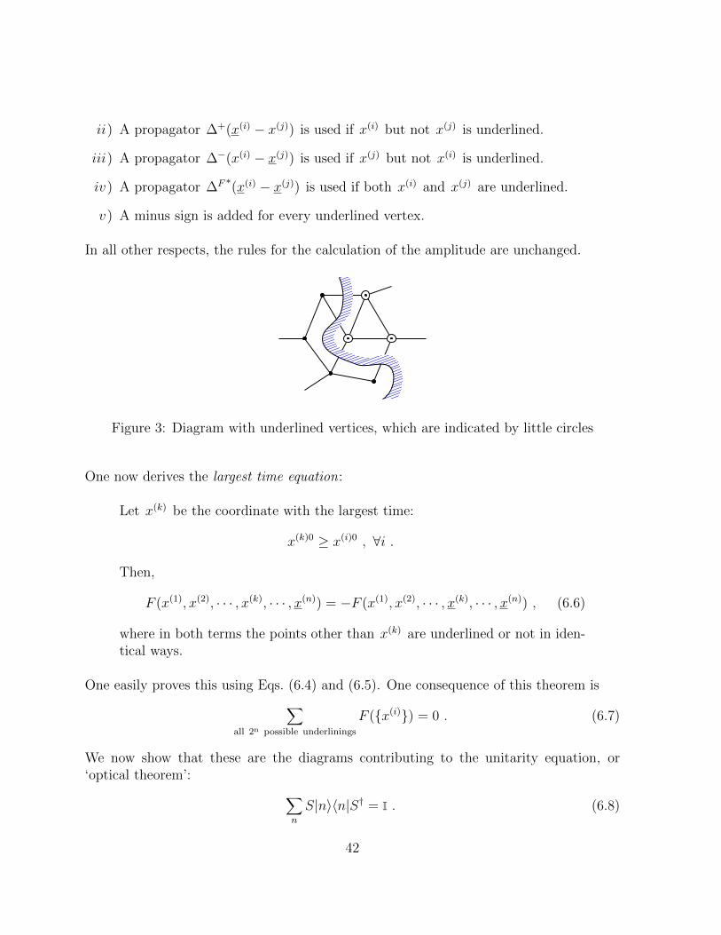
ii) A propagator ∆+(x(i) − x(j)) is used if x(i) but not x(j) is underlined.

iii) A propagator ∆−(x(i) − x(j)) is used if x(j) but not x(i) is underlined.

iv ) A propagator ∆F ∗(x(i) − x(j)) is used if both x(i) and x(j) are underlined.

v ) A minus sign is added for every underlined vertex.

In all other respects, the rules for the calculation of the amplitude are unchanged.

Figure 3: Diagram with underlined vertices, which are indicated by little circles

One now derives the largest time equation:

Let x(k) be the coordinate with the largest time:

x(k)0 ≥ x(i)0 , ∀i .

Then,

F (x(1), x(2), · · · , x(k), · · · , x(n)) = −F (x(1), x(2), · · · , x(k), · · · , x(n)) , (6.6)

where in both terms the points other than x(k) are underlined or not in iden-tical ways.

One easily proves this using Eqs. (6.4) and (6.5). One consequence of this theorem is∑all 2n possible underlinings

F (x(i)) = 0 . (6.7)

We now show that these are the diagrams contributing to the unitarity equation, or‘optical theorem’: ∑

n

S|n〉〈n|S† = I . (6.8)

42

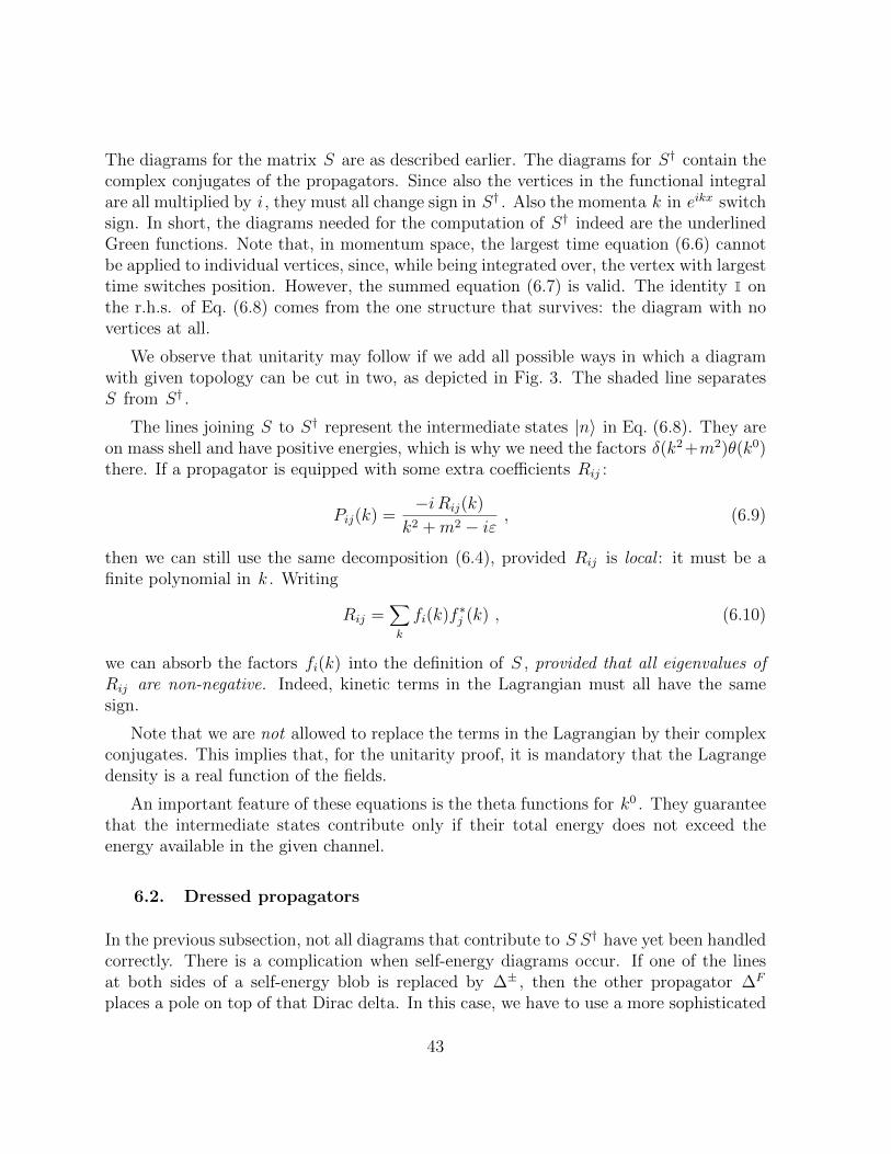
The diagrams for the matrix S are as described earlier. The diagrams for S† contain thecomplex conjugates of the propagators. Since also the vertices in the functional integralare all multiplied by i , they must all change sign in S† . Also the momenta k in eikx switchsign. In short, the diagrams needed for the computation of S† indeed are the underlinedGreen functions. Note that, in momentum space, the largest time equation (6.6) cannotbe applied to individual vertices, since, while being integrated over, the vertex with largesttime switches position. However, the summed equation (6.7) is valid. The identity I onthe r.h.s. of Eq. (6.8) comes from the one structure that survives: the diagram with novertices at all.

We observe that unitarity may follow if we add all possible ways in which a diagramwith given topology can be cut in two, as depicted in Fig. 3. The shaded line separatesS from S† .

The lines joining S to S† represent the intermediate states |n〉 in Eq. (6.8). They areon mass shell and have positive energies, which is why we need the factors δ(k2 +m2)θ(k0)there. If a propagator is equipped with some extra coefficients Rij :

Pij(k) =−i Rij(k)

k2 +m2 − iε, (6.9)

then we can still use the same decomposition (6.4), provided Rij is local : it must be afinite polynomial in k . Writing

Rij =∑k

fi(k)f ∗j (k) , (6.10)

we can absorb the factors fi(k) into the definition of S , provided that all eigenvalues ofRij are non-negative. Indeed, kinetic terms in the Lagrangian must all have the samesign.

Note that we are not allowed to replace the terms in the Lagrangian by their complexconjugates. This implies that, for the unitarity proof, it is mandatory that the Lagrangedensity is a real function of the fields.

An important feature of these equations is the theta functions for k0 . They guaranteethat the intermediate states contribute only if their total energy does not exceed theenergy available in the given channel.

6.2. Dressed propagators

In the previous subsection, not all diagrams that contribute to S S† have yet been handledcorrectly. There is a complication when self-energy diagrams occur. If one of the linesat both sides of a self-energy blob is replaced by ∆± , then the other propagator ∆F

places a pole on top of that Dirac delta. In this case, we have to use a more sophisticated

43

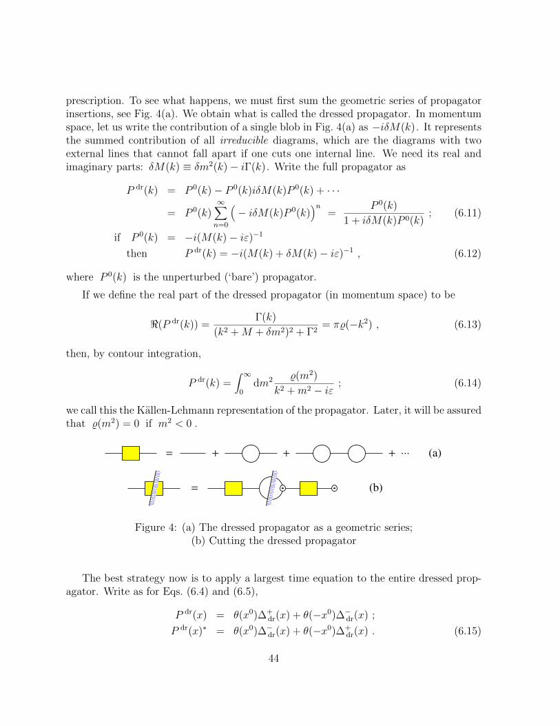
prescription. To see what happens, we must first sum the geometric series of propagatorinsertions, see Fig. 4(a). We obtain what is called the dressed propagator. In momentumspace, let us write the contribution of a single blob in Fig. 4(a) as −iδM(k). It representsthe summed contribution of all irreducible diagrams, which are the diagrams with twoexternal lines that cannot fall apart if one cuts one internal line. We need its real andimaginary parts: δM(k) ≡ δm2(k)− iΓ(k). Write the full propagator as

P dr(k) = P 0(k)− P 0(k)iδM(k)P 0(k) + · · ·

= P 0(k)∞∑n=0

(− iδM(k)P 0(k)

)n=

P 0(k)

1 + iδM(k)P 0(k); (6.11)

if P 0(k) = −i(M(k)− iε)−1

then P dr(k) = −i(M(k) + δM(k)− iε)−1 , (6.12)

where P 0(k) is the unperturbed (‘bare’) propagator.

If we define the real part of the dressed propagator (in momentum space) to be

<(P dr(k)) =Γ(k)

(k2 +M + δm2)2 + Γ2= π%(−k2) , (6.13)

then, by contour integration,

P dr(k) =∫ ∞

0dm2 %(m2)

k2 +m2 − iε; (6.14)

we call this the Kallen-Lehmann representation of the propagator. Later, it will be assuredthat %(m2) = 0 if m2 < 0 .

= + + + ⋅⋅⋅ (a)

= (b)

Figure 4: (a) The dressed propagator as a geometric series;(b) Cutting the dressed propagator

The best strategy now is to apply a largest time equation to the entire dressed prop-agator. Write as for Eqs. (6.4) and (6.5),

P dr(x) = θ(x0)∆+dr(x) + θ(−x0)∆−dr(x) ;

P dr(x)∗ = θ(x0)∆−dr(x) + θ(−x0)∆+dr(x) . (6.15)

44

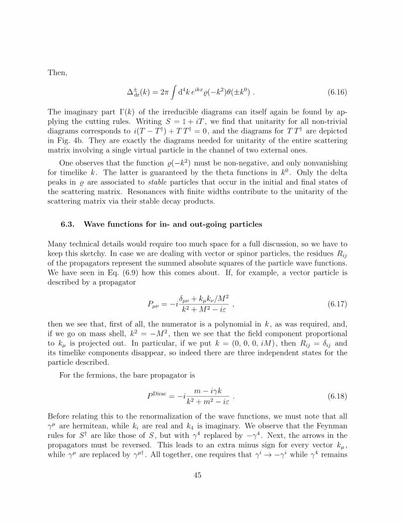
Then,

∆±dr(k) = 2π∫

d4k eikx%(−k2)θ(±k0) . (6.16)

The imaginary part Γ(k) of the irreducible diagrams can itself again be found by ap-plying the cutting rules. Writing S = I + iT , we find that unitarity for all non-trivialdiagrams corresponds to i(T − T †) + T T † = 0, and the diagrams for T T † are depictedin Fig. 4b. They are exactly the diagrams needed for unitarity of the entire scatteringmatrix involving a single virtual particle in the channel of two external ones.

One observes that the function %(−k2) must be non-negative, and only nonvanishingfor timelike k . The latter is guaranteed by the theta functions in k0 . Only the deltapeaks in % are associated to stable particles that occur in the initial and final states ofthe scattering matrix. Resonances with finite widths contribute to the unitarity of thescattering matrix via their stable decay products.

6.3. Wave functions for in- and out-going particles

Many technical details would require too much space for a full discussion, so we have tokeep this sketchy. In case we are dealing with vector or spinor particles, the residues Rij

of the propagators represent the summed absolute squares of the particle wave functions.We have seen in Eq. (6.9) how this comes about. If, for example, a vector particle isdescribed by a propagator

Pµν = −iδµν + kµkν/M2

k2 +M2 − iε, (6.17)

then we see that, first of all, the numerator is a polynomial in k , as was required, and,if we go on mass shell, k2 = −M2 , then we see that the field component proportionalto kµ is projected out. In particular, if we put k = (0, 0, 0, iM), then Rij = δij andits timelike components disappear, so indeed there are three independent states for theparticle described.

For the fermions, the bare propagator is

PDirac = −i m− iγkk2 +m2 − iε

. (6.18)

Before relating this to the renormalization of the wave functions, we must note that allγµ are hermitean, while ki are real and k4 is imaginary. We observe that the Feynmanrules for S† are like those of S , but with γ4 replaced by −γ4 . Next, the arrows in thepropagators must be reversed. This leads to an extra minus sign for every vector kµ ,while γµ are replaced by 㵆 . All together, one requires that γi → −γi while γ4 remains

45

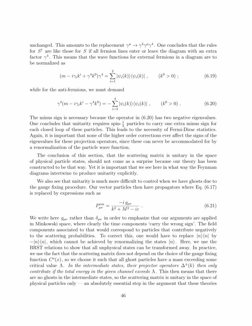
unchanged. This amounts to the replacement γµ → γ4γµγ4 . One concludes that the rulesfor S† are like those for S if all fermion lines enter or leave the diagram with an extrafactor γ4 . This means that the wave functions for external fermions in a diagram are tobe normalized as

(m− iγiki + γ4k0)γ4 =2∑i=1

|ψi(k)〉〈ψi(k)| , (k0 > 0) ; (6.19)

while for the anti-fermions, we must demand

γ4(m− iγiki − γ4k0) = −4∑i=3

|ψi(k)〉〈ψi(k)| , (k0 > 0) . (6.20)

The minus sign is necessary because the operator in (6.20) has two negative eigenvalues.One concludes that unitarity requires spin- 1

2particles to carry one extra minus sign for

each closed loop of these particles. This leads to the necessity of Fermi-Dirac statistics.Again, it is important that none of the higher order corrections ever affect the signs of theeigenvalues for these projection operators, since these can never be accommodated for bya renormalization of the particle wave function.

The conclusion of this section, that the scattering matrix is unitary in the spaceof physical particle states, should not come as a surprise because our theory has beenconstructed to be that way. Yet it is important that we see here in what way the Feynmandiagrams intertwine to produce unitarity explicitly.

We also see that unitarity is much more difficult to control when we have ghosts due tothe gauge fixing procedure. Our vector particles then have propagators where Eq. (6.17)is replaced by expressions such as

P renµν =

−i gµνk2 +M2 − iε

. (6.21)

We write here gµν rather than δµν in order to emphasize that our arguments are appliedin Minkowski space, where clearly the time components ‘carry the wrong sign’. The fieldcomponents associated to that would correspond to particles that contribute negativelyto the scattering probabilities. To correct this, one would have to replace |n〉〈n| by−|n〉〈n| , which cannot be achieved by renormalizing the states |n〉 . Here, we use theBRST relations to show that all unphysical states can be transformed away. In practice,we use the fact that the scattering matrix does not depend on the choice of the gauge fixingfunction Ca(x), so we choose it such that all ghost particles have a mass exceeding somecritical value Λ. In the intermediate states, their projector operators ∆±(k) then onlycontribute if the total energy in the given channel exceeds Λ. This then means that thereare no ghosts in the intermediate states, so the scattering matrix is unitary in the space ofphysical particles only — an absolutely essential step in the argument that these theories

46

are internally consistent. The required gauge fixing functions Ca(x) are not difficult toconstruct, but their existence is only needed to complete this formal argument. They arerather cumbersome to use in practical calculations.

6.4. Dispersion relations

The largest time equation can also be employed to derive very important dispersion rela-tions for the diagrams. These imply that any diagram D can be regarded as a combinationof two sets of diagrams Di and D†i :

D =∑i

∫ ∞0

dk0

−k0 − iεDi(k

0)D†i (k0) . (6.22)

Here, Di(k0) and D†i (k

0) stand for amplitudes depending on various external momentak , where one of the timelike components, k0 , is integrated over. This, one derives bysingling out two points, x(1) and x(2) in a diagram, and time-ordering them. The detailsof the derivation go beyond the scope of this paper (although they are not more difficultthan the previous derivations in this section). Eq. (6.22) can be used to express diagramswith closed loops in terms of diagrams with fewer closed loops, and discuss the subtractionprocedures needed for renormalization.

7. Renormalization

For a proper discussion of the renormalization concept, we must emphasize what ourstarting point was: first, replace the continuum of space by a dense lattice of points, andonly at the very end of all calculations do we make an attempt to take the continuum limit.The path integral procedure, illuminated in subsection 2.4, implies that time, also, canbe replaced by a lattice. In Fourier space, the space-time lattice leads to finite domainsfor the values of energies and momenta (the Brillouin zones), so that all ultra-violetdivergences disappear. If we also wish to ensure the absence of infra-red divergences, wemust replace the infinite volume of space and time by a finite box. This is often requiredif complications arise due to divergent contributions of soft virtual particles, typicallyphotons. Nasty infra-red divergences occur in theories with confinement, to be discussedin section 11.

The instruments that we shall use for the ultra-violet divergences of a theory are asfollows. We assume that all freely adjustable physical constants of the theory, referredto as the ‘bare’ parameters, such as the ’bare’ mass and charge of a particle, should becarefully tuned to agree with observation, but the tuning process may depend criticallyon the mesh size a of the space-time lattice. Thus, while we vary a , we allow all bare

47

parameters, λ say, in the theories to depend on a , often tending either to infinity or tozero as a→ 0. If this procedure is combined with a perturbation expansion, say in termsof a small coupling g , we expect to find that observable features depend minimally on aprovided that the bare couplings g(a) remain small in the limit a ↓ 0.

This will be an important condition for our theories to make sense at all. How do weknow whether g(a) tends to zero or not? The simplest thing to look at, is the dimension-ality of g . All parameters of a field theory have a dimension of a length to some power.These dimensions usually depend on the dimensionality n of space-time. The rules tocompute them are easy to obtain:

- An action S =∫

dnxL(x) is dimensionless;

- The dimension of a Lagrange density L is therefore (length)−n = mn , where m isa mass.

- The dimension of the fields can be read off from the kinetic terms in the Lagrangian,because they contain no further parameters. A scalar field φ has dimension m(n−2)/2 ,a fermionic field ψ has dimension m(n−1)/2 .

- A gauge coupling constant g has dimension m(4−n)/2 and the coupling parameter λin an interaction term of the form λφk has dimension mn+k−nk/2 ,

and so on.

A theory is called power-counting renormalizable, if all expansion parametershave mass-dimension positive or zero.

This is why, in 4 space-time dimensions, we cannot accept higher than quartic interac-tions among scalars. In practice, in 4 space-time dimensions, most expansion parametershave dimension zero. In Section 9, we will see that dimensionless coupling parametersnevertheless depend on the size of a , but only logarithmically:

λ(a) ≈ λ0 + Cλ20 log(a) + higher orders. (7.1)

Regardless of whether this tends to zero or to infinity in the continuum limit, one findsthat, in the continuum theory, the perturbative corrections to the bare parameters λdiverge. This is nothing to be alarmed about. However, if λ itself is also a small parameterin terms of which we wish to perform a perturbation expansion, then clearly trouble isto be expected if its bare value tends to infinity. Indeed, we shall argue that, in general,such theories are inconsistent.

There are two very important remarks to be made:

48

— Theories can be constructed where all couplings really tend to zero in the continuumlimit. These theories are called asymptotically free (Section 9), and they allow foraccurate approximations in the ultra-violet. It is generally believed that such theo-ries can be defined in a completely unambiguous fashion through their perturbationexpansions in the ultra-violet; in any case, they allow for very accurate calculationof all their physical properties. QCD is the prime example.

— If a theory is not asymptotically free, but has only small coupling parameters, theperturbation expansion formally diverges, and the continuum limit formally does notexist. But the first N terms of perturbation expansion do make sense, where N =O(1/g). This means that uncontrollable margins of error are exponentially small, oforder e−C/g or e−C/g

2, which in practice is much smaller than other uncertainties in

the theory, so they are of hardly any practical consequence. Thus, in such a case, ourtheory does have intrinsic inaccuracies, but these are exponentially suppressed. Inpractice, such theories are still highly valuable. The Standard Model is an example.

A useful approach is to substitute all numbers in a theory by formal series expansions,where the expansion parameter, a factor common to all coupling parameters of the theory,is formally kept infinitesimal. In that case, all perturbation coefficients are uniquelydefined, though one has little direct knowledge concerning the convergence or divergenceof the expansions.

In both the cases mentioned above, our theories are defined from their perturba-tion expansion; clearly, the perturbation expansion is not only a convenient device forcalculations, it is an essential ingredient in our theories. Let us therefore study howrenormalization works, order-by-order in perturbation theory.

In a connected diagram, let the number of external lines be E , the number of propa-gators be P , and let Vn be the number of vertices with n prongs. By drawing two dotson each propagator and one on each external line, one finds that the number of dots is

2P + E =∑n

nVn = 3V3 + 4V4. (7.2)

For tree diagrams (simply connected diagrams), one finds by induction, with V the num-ber of vertices, V =

∑n Vn ,

V = P + 1 . (7.3)

A diagram with L closed loops (an L-fold connected diagram) turns into a tree by cuttingaway L propagators. Therefore, one has

P = V − 1 + L . (7.4)

49

Combining Eqs. (7.2) and (7.4), one has

E + 2L− 2 =∑n

(n− 2)Vn = V3 + 2V4 . (7.5)

Consequently, if every 3-vertex comes with a factor g and every 4-vertex with a factor λ ,and if a diagram with a given number E of external lines, behaves as g2nλk , it must haveL = n + k + 1 − 1

2E closed loops. Perturbation expansion is therefore often regarded as

an expansion in terms of the number of closed loops.

7.1. Regularization schemes

In a tree diagram, in momentum space, no integrations are needed to be done — themomentum flowing through every propagator is fixed by the momenta of the in- andout-going particles. But if there are L loops, one has to perform 4L integrations inmomentum space. It is these integrations that often tend to diverge at large momenta.

Of course, these divergences are stopped if momentum space is cut off, as is the casein a finite lattice. However, since our lattice is not Lorentz-invariant and may lack othersymmetries such as gauge-invariance, it is useful to find other ways to modify our theoryso that UV divergences disappear. This is called ‘regularization’. We give two examples.

7.1.1. Pauli-Villars regularization

Assume that a propagator of the form shown is replaced as follows:

A(k)

k2 +m2 − iε→

∑i

eiA(k)

k2 + Λ2i − iε

;∑i

ei = 0 ,∑i

eiΛ2i = 0 . (7.6)

If we take e1 = 1, Λ1 = m , while all other Λi tend to +∞ , we get back the originalpropagator. With finite Λi , however, we can make all momentum integrations converge atinfinity. Our theory is then finite. This is (a somewhat simplified version of) Pauli-Villarsregularization.

However, the new propagators cannot describe ordinary particles. The ones withei < 0 contribute to the unitarity relation with the wrong sign! On the other hand, theiε prescription is as usual, so that these particles do carry positive energy. In any channelwhere the total energy is less than Λi , the ‘Pauli-Villars ghosts’ do not contribute tothe unitarity relation at all. So, in a theory where we put a limit to the total energyconsidered, Pauli-Villars regularization is physically acceptable. In practice, we will tryto send all ghost masses Λi to infinity.

50

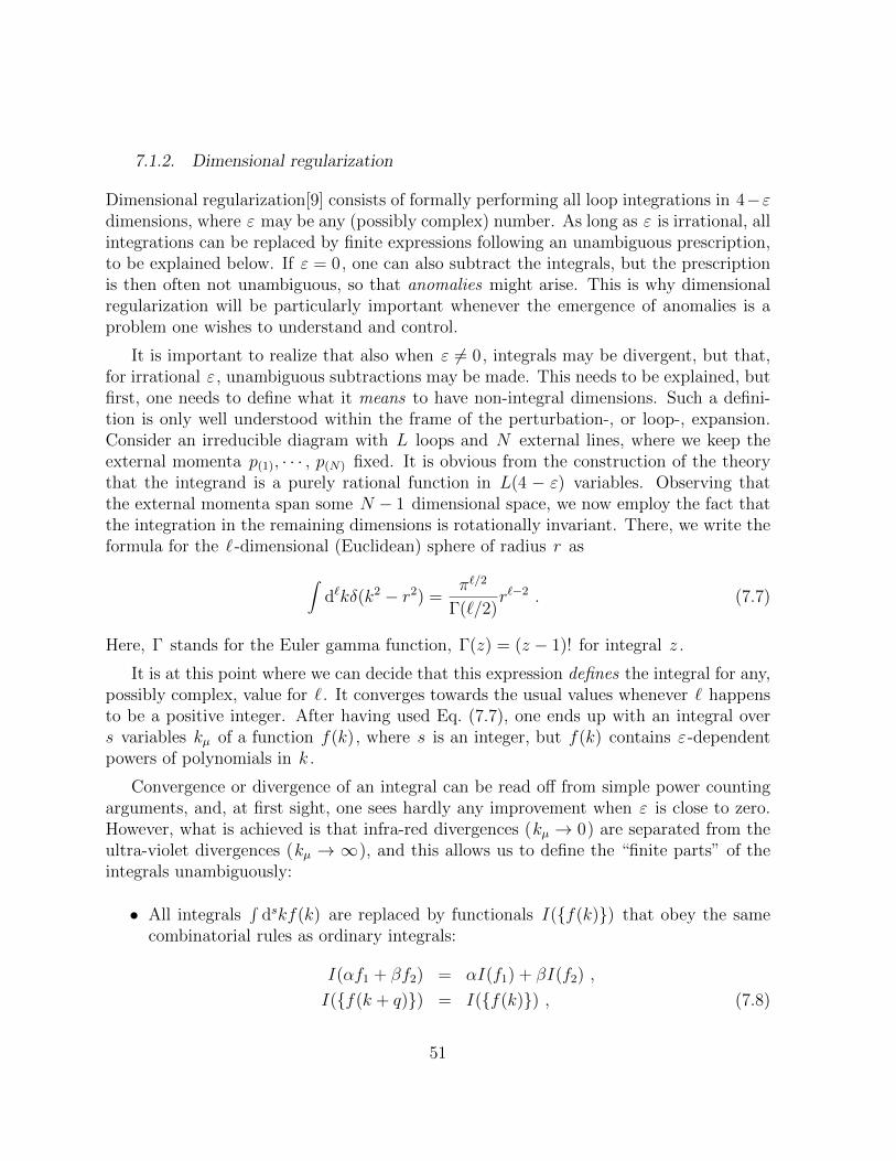
7.1.2. Dimensional regularization

Dimensional regularization[9] consists of formally performing all loop integrations in 4−εdimensions, where ε may be any (possibly complex) number. As long as ε is irrational, allintegrations can be replaced by finite expressions following an unambiguous prescription,to be explained below. If ε = 0, one can also subtract the integrals, but the prescriptionis then often not unambiguous, so that anomalies might arise. This is why dimensionalregularization will be particularly important whenever the emergence of anomalies is aproblem one wishes to understand and control.

It is important to realize that also when ε 6= 0, integrals may be divergent, but that,for irrational ε , unambiguous subtractions may be made. This needs to be explained, butfirst, one needs to define what it means to have non-integral dimensions. Such a defini-tion is only well understood within the frame of the perturbation-, or loop-, expansion.Consider an irreducible diagram with L loops and N external lines, where we keep theexternal momenta p(1), · · · , p(N) fixed. It is obvious from the construction of the theorythat the integrand is a purely rational function in L(4 − ε) variables. Observing thatthe external momenta span some N − 1 dimensional space, we now employ the fact thatthe integration in the remaining dimensions is rotationally invariant. There, we write theformula for the `-dimensional (Euclidean) sphere of radius r as

∫d`kδ(k2 − r2) =

π`/2

Γ(`/2)r`−2 . (7.7)

Here, Γ stands for the Euler gamma function, Γ(z) = (z − 1)! for integral z .

It is at this point where we can decide that this expression defines the integral for any,possibly complex, value for ` . It converges towards the usual values whenever ` happensto be a positive integer. After having used Eq. (7.7), one ends up with an integral overs variables kµ of a function f(k), where s is an integer, but f(k) contains ε-dependentpowers of polynomials in k .

Convergence or divergence of an integral can be read off from simple power countingarguments, and, at first sight, one sees hardly any improvement when ε is close to zero.However, what is achieved is that infra-red divergences (kµ → 0) are separated from theultra-violet divergences (kµ → ∞), and this allows us to define the “finite parts” of theintegrals unambiguously:

• All integrals∫

dskf(k) are replaced by functionals I(f(k)) that obey the samecombinatorial rules as ordinary integrals:

I(αf1 + βf2) = αI(f1) + βI(f2) ,

I(f(k + q)) = I(f(k)) , (7.8)

51

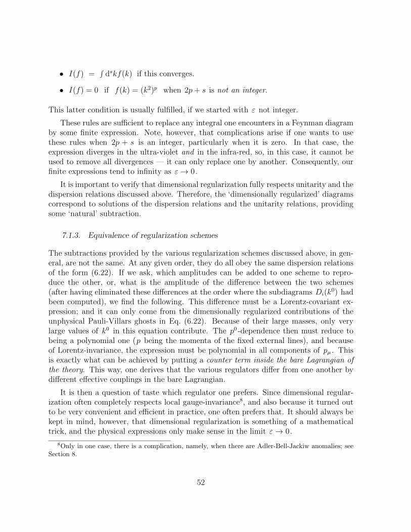
• I(f) =∫

dskf(k) if this converges.

• I(f) = 0 if f(k) = (k2)p when 2p+ s is not an integer.

This latter condition is usually fulfilled, if we started with ε not integer.

These rules are sufficient to replace any integral one encounters in a Feynman diagramby some finite expression. Note, however, that complications arise if one wants to usethese rules when 2p + s is an integer, particularly when it is zero. In that case, theexpression diverges in the ultra-violet and in the infra-red, so, in this case, it cannot beused to remove all divergences — it can only replace one by another. Consequently, ourfinite expressions tend to infinity as ε→ 0.

It is important to verify that dimensional regularization fully respects unitarity and thedispersion relations discussed above. Therefore, the ‘dimensionally regularized’ diagramscorrespond to solutions of the dispersion relations and the unitarity relations, providingsome ‘natural’ subtraction.

7.1.3. Equivalence of regularization schemes

The subtractions provided by the various regularization schemes discussed above, in gen-eral, are not the same. At any given order, they do all obey the same dispersion relationsof the form (6.22). If we ask, which amplitudes can be added to one scheme to repro-duce the other, or, what is the amplitude of the difference between the two schemes(after having eliminated these differences at the order where the subdiagrams Di(k

0) hadbeen computed), we find the following. This difference must be a Lorentz-covariant ex-pression; and it can only come from the dimensionally regularized contributions of theunphysical Pauli-Villars ghosts in Eq. (6.22). Because of their large masses, only verylarge values of k0 in this equation contribute. The p0 -dependence then must reduce tobeing a polynomial one (p being the momenta of the fixed external lines), and becauseof Lorentz-invariance, the expression must be polynomial in all components of pµ . Thisis exactly what can be achieved by putting a counter term inside the bare Lagrangian ofthe theory. This way, one derives that the various regulators differ from one another bydifferent effective couplings in the bare Lagrangian.

It is then a question of taste which regulator one prefers. Since dimensional regular-ization often completely respects local gauge-invariance8, and also because it turned outto be very convenient and efficient in practice, one often prefers that. It should always bekept in mind, however, that dimensional regularization is something of a mathematicaltrick, and the physical expressions only make sense in the limit ε→ 0.

8Only in one case, there is a complication, namely, when there are Adler-Bell-Jackiw anomalies; seeSection 8.

52

7.2. Renormalization of gauge theories

Using the results from the previous Sections, we decide to treat quantum field theoriesin general, and gauge theories in particular, as follows: first, we regularize the theory,by using a ‘lattice cut-off’, or a Pauli-Villars cut-off, or by turning towards n = 4 − εdimensions. All these procedures are characterized by a small parameter, such as ε , suchthat the physical theory is formally obtained in the limit ε → 0. These procedures areall equivalent, in the sense that by adding local interaction terms to the Lagrangian, onecan map the results of one scheme onto those of another. Subsequently, we renormalizethe theory. This means that all parameters in the Lagrangian are modified by finitecorrections, which however may diverge in the limit ε → 0. If these counter terms havebeen chosen well, the theory may stay finite and well defined in this limit. In particular,we should have a unitary, causal theory.

Unitarity is only guaranteed if the theory is gauge-invariant. Therefore, one prefersregulator schemes that preserve gauge-invariance throughout. This is what dimensionalregularization often does. In that case, the renormalization procedure respects BRST-invariance, see Subsect. 4.5.

8. Anomalies

The Sections that follow will (again) be too brief to form a complete text for learningQuantum Field Theory. Our aim is here to give a summary of the features that are allextremely important to understand the general structure of relativistic Quantum FieldTheories.

If, for a given theory, no obviously gauge-invariant regularization procedure appearsto exist, this might be for a reason: such a theory might not be renormalizable at all. Inprinciple, this could be checked, as follows. One may always decide to use a regularizationprocedure that does not respect the symmetries one wants, provided that the symmetrycan be restored in the limit where the physically observable effects of the regulator goaway, such as ε → 0, or Λi → ∞, i > 0. If a gauge-invariant regulator does exist,but it hasn’t yet been explicitly constructed, then we know that it differs from any otherregulator by a bunch of finite counter terms. To find such counter terms is not hard, inpractice; just add all terms needed to restore BRST invariance of the amplitudes.

But, in case that regulator is not known, how can we then be sure that such termsexist at all? BRST invariance requires the validity of the Slavnov-Taylor identities, butthey appear to overdetermine the subtraction terms. This is the way we originally phrasedthe problem in Ref. [14]. In fact, indeed there may be a clash. If this happens, it is calledan anomaly.[20]

53

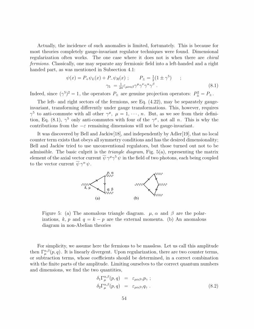
Actually, the incidence of such anomalies is limited, fortunately. This is because formost theories completely gauge-invariant regulator techniques were found. Dimensionalregularization often works. The one case where it does not is when there are chiralfermions. Classically, one may separate any fermionic field into a left-handed and a righthanded part, as was mentioned in Subsection 4.1:

ψ(x) = P+ψL(x) + P−ψR(x) ; P± = 12(1± γ5) ;

γ5 = 124εµναβγ

µγνγαγβ . (8.1)

Indeed, since (γ5)2 = 1, the operators P± are genuine projection operators: P 2± = P± .

The left- and right sectors of the fermions, see Eq. (4.22), may be separately gauge-invariant, transforming differently under gauge transformations. This, however, requiresγ5 to anti-commute with all other γµ, µ = 1, · · · , n . But, as we see from their defini-tion, Eq. (8.1), γ5 only anti-commutes with four of the γµ , not all n . This is why thecontributions from the −ε remaining dimensions will not be gauge-invariant.

It was discovered by Bell and Jackiw[18], and independently by Adler[19], that no localcounter term exists that obeys all symmetry conditions and has the desired dimensionality;Bell and Jackiw tried to use unconventional regulators, but those turned out not to beadmissible. The basic culprit is the triangle diagram, Fig. 5(a), representing the matrixelement of the axial vector current ψ γµγ5 ψ in the field of two photons, each being coupledto the vector current ψ γα ψ .

(b)(a)

k, µ

p, α

q, β

Figure 5: (a) The anomalous triangle diagram. µ, α and β are the polar-izations, k, p and q = k − p are the external momenta. (b) An anomalousdiagram in non-Abelian theories

For simplicity, we assume here the fermions to be massless. Let us call this amplitudethen Γα,βµ (p, q). It is linearly divergent. Upon regularization, there are two counter terms,or subtraction terms, whose coefficients should be determined, in a correct combinationwith the finite parts of the amplitude. Limiting ourselves to the correct quantum numbersand dimensions, we find the two quantities,

δ1Γα,βµ (p, q) = εµαβγpγ ;

δ2Γα,βµ (p, q) = εµαβγqγ . (8.2)

54

We can determine their coefficients by applying the condition that the total amplitude beinvariant under gauge transformations of the photon field. This implies that the expressionmust vanish when any of the two photons are longitudinal: Aµ = ∂µΛ, which means

pαΓα,βµ (p, q) = 0 ; qβΓα,βµ (p, q) = 0 . (8.3)

Since

pαδ1Γα,βµ (p, q) = 0 ; qβδ1Γα,βµ (p, q) = Aµ,α ;

pαδ2Γα,βµ (p, q) = Aµ,β ; qβδ2Γα,βµ (p, q) = 0 ; (8.4)

Aµ,α = εµαβγpγqβ ,

this fixes the coefficients in front of δ1Γ and δ2Γ.

When now we investigate whether this amplitude is also transversal with respect to theaxial vector current, we are struck by a surprise. The counter terms, fixed by condition(8.4), also contribute here:

kµδ1Γα,βµ (p, q) = −kµδ2Γα,βµ (p, q) = Aα,β , (8.5)

but they do not cancel against the contribution of the finite part. After imposing gauge-invariance with respect to the two vector insertions, one finds (in the case of a single chiralfermion)

kµΓα,βµ (p, q) = (4π2)−1εµαβγpµqγ , (8.6)

and this can be rewritten as an effective divergence property of a vector current:

∂µJ5µ = −iLe

2

8π2FµνFµν , (8.7)

where Fµν = 12εµναβFαβ , and it was assumed that the photons couple with charges e .

What is surprising about this is, that the triangle diagram itself, Fig. 5a, appears to betotally symmetric under all permutations, since γ5 can be permuted to any of the otherend-points. Imposing gauge-invariance at two of its three end-points implies breaking ofthe invariance at the third.

This result is very important. It implies an induced violation of a conservation law,apparently to be attributed to the regularization procedure. It also means that it is notpossible to couple three gauge bosons to such a triangle graph, because this cannot bedone in a gauge-invariant way. In most theories, however, we have couplings both toleft-handed and to right-handed fermions. Their contributions are of opposite sign, whichmeans that they can cancel out. Therefore, one derives an important constraint on gaugetheories with chiral fermions: The triangle anomalies must cancel out.

55

Let the left handed chiral fermions be in representations of the total set of gaugegroups that transform as

ψiL → ψiL + iΛaT aLijψ

jL (8.8)

where Λ is infinitesimal, and T aL are the gauge generators for the left-handed fermions.Similarly for the right-handed ψiR . Define

dabcL = Tr(T aLTbLT

cL + T bLT

aLT

cL) , (8.9)

and similarly dabcR . The anomaly constraint is then∑dabcL =

∑dabcR , (8.10)

where the sum is over all fermion species in the theory. In the Standard Model, theonly contributions could come if either one or all three indices of dabc refer to the U(1)group. One quickly verifies that indeed the U(1) charges of the quarks and leptons aredistributed in such a way that (8.10) is completely verified, but only if the number of quarkgenerations and lepton generations are equal. In Chapter 10.3, we will see the physicalsignificance of this observation.

Note, that in the non-Abelian case, there are also anomalies in diagrams with 4 externallegs, see Fig. 5(b). They arise from the trilinear terms in FµνFµν (the quadrilinear termscancel). These are the only cases where the regularization procedure may violate gaugeinvariance. In diagrams with more loops, or sub diagrams with more external lines,regularization procedures could be found that preserve gauge invariance.

9. Asymptotic freedom

9.1. The Renormalization Group

It was observed by Stueckelberg and Peterman[21] in 1953, that, although the perturbativeexpansion of a theory depends on how one splits up the bare parameters in the Lagrangianinto lowest order parameters, and counter terms required for the renormalization, theentire theory should not depend on this. This they interpreted as an invariance, and theaction of replacing parameters from lowest order to higher order corrections as a groupoperation. One obtains the ‘Renormalization Group’.

There is only one instance where such transformtions really matter, and that is whenone compares a theory at one mass- or distance-scale to the same theory at a different scale.A scale transformation must be associated with a replacement of counter terms. Thus,physicists began to identify the notion of a scale transformation as a ‘renormalizationgroup transformation’.

56

Gell-Mann and Low[22] observed that this procedure can be used to derive the small-distance behavior of QED. One finds that the effective fine-structure constant depends onthe scale µ , described by the equation

µ2d

dµ2α(µ) = β(α) =

α2N

3π+O(α3) , (9.1)

where N is the number of charged fermion types. As long as α(µ) stays small, so thatthe O(α3) terms can be neglected, we see that its µ-dependence is

α(µ) =α0

1− (α0N/3π) log(µ2/µ20), if α(µ0) = α0 . (9.2)

Things run out of control when µ reaches values comparable to exp(3π/2Nα0), but, atleast in the case of QED, where α0 ≈ 1/137, this mass scale is so large that in practice noproblems are expected. The pole in Eq. (9.2) is called the Landau pole; Landau concludedthat quantum field theories such as QED have no true continuum limit because of thispole. Gell-Mann and Low suspected, however, that β(α) might have a zero at some largevalue of α , so that, at high values of µ , α approaches this value, but does not exceedthis stationary point.

What exactly happens at or near the Landau pole, cannot be established using per-turbation expansion alone, since this will depend on all higher order terms in Eq. (9.1); infact, it is not even known whether Quantum Field Theory can be reformulated accuratelyenough to decide. The question, however, might be not as important as it seems, sincethe Landau pole will be way beyond the Planck mass, where we know that gravitationalterms will take over; it will be more important to solve Quantum Gravity first.

An entirely different situation emerges in theories where the function β(λ) is negative.It was long thought that this situation can never arise, unless the coupling strength λitself is given the wrong sign (the sign that would render the energy density of the classicaltheory unbounded from below), but this turns out only to be the case in theories thatonly contain scalar and spinor fields. If there is a non-Abelian Yang-Mills component inthe theory, negative β functions do occur. In the simplest case, an SU(2) gauge theorywith Nf fermions in the elementary doublet representation, the beta function is

µ2d

dµ2g2(µ) = β(g2) =

Nf − 11

24π2g4(µ) +O(g6) , (9.3)

so, as long as Nf < 11 we have that the coupling strength g(µ) tends to zero, logarithmi-cally, as µ→∞ . This feature is called asymptotic freedom. In an SU(Nc) gauge theory,the β function is proportional to Nf − 11

2Nc , so, with the present number of Nf = 6

quark flavors, QCD (Nc = 3) is asymptotically free. In line with a notation often used,the subscript c here stands for ”colour”; in QCD, the number of colours is Nc = 3.

57

9.2. An algebra for the beta functions

In theories with gauge fields, fermions, and scalars, the situation is more complex. Ageneral algorithm for the beta functions has been worked out. The most compact notationfor the general result can be given by writing how the entire Lagrange density L scalesunder a scale transformation. Let the Lagrangian L be

L = −14GaµνG

aµν − 1

2(Dµφi)

2 − V (φ)− ψiγµDµψi

−ψi(Sij(φ) + iγ5Pij(φ)

)ψj , (9.4)

where the covariant derivatives are defined as follows:9

Dµφi ≡ ∂µφi + iT aijAaµφj ; Dµψi = ∂µψi + iUa

ijAaµψj , (9.5)

and the structure constants fabc are defined by

[T a, T b] = −ifabcTc , (9.6)

so that

Gaµν = ∂µA

aν − ∂νAaµ + fabcAbµA

cν . (9.7)

We split the fermions into right- and left-handed representations, so that

Ua = UaLPL + Ua

RPR ; PL =1 + γ5

2, PR =

1− γ5

2. (9.8)

The functions S(φ) and P (φ) are at most linear in φ and V (φ) is at most quartic. TheLagrangian (9.4) is the gauge-invariant part; we do not write the gauge-fixing part or theghost; the final result will not depend on those details.

The result of an algebraical calculation is that

16π2µ2dLdµ2

=

GaµνG

bµν [−

11

12Cab

1 +1

24Cab

2 +1

6Cab

3 ]−∆V − ψ(∆S + iγ5∆P )ψ , (9.9)

in which

Cab1 = fapqf bpq , (9.10)

Cab2 = Tr (T aT b) , (9.11)

Cab3 = Tr (Ua

LUbL + Ua

RUbR) , (9.12)

∆V = 14V 2ij − 3

2Vi(T

2φ)i + 34(φT aT bφ)2

+φiVjTr (S,iS,j + P,iP,j)− Tr (S2 + P 2)2 + Tr [S, P ]2 , (9.13)

9T and U are hermitean, but since φ is real, the elements of T must be imaginary.

58

where

Vi ≡∂V (φ)

∂φi; S,i ≡

∂S

∂φi, etc., (9.14)

and writing S + iP = W , one finds ∆S and ∆P from

∆W = 14WiW

∗i W + 1

4WW ∗

i Wi +WiW∗Wi

−32(U2

RW )− 32W (UL)2 +WiφjTr (SiSj + PiPj) . (9.15)

This expression does not include information on how fields φi and ψi transform underscaling. The fields are not directly observable.

This algebraic expression can be used to find how, in general, coupling strengths rununder rescalings of the momenta. It is an interesting exercise to work out what theconditions are for asymptotic freedom, that is, for all coupling strengths to run to zero atinfinite momentum. In general, one finds that scalar fields can only exist if there are alsogauge fields and fermions present; the latter must be in sufficiently high representationsof the gauge group.

10. Topological Twists

The Lagrangian (9.4) is the most general one allowed if we wish to limit ourselves tocoupling strengths that run logarithmically under rescalings of the momenta, see for in-stance Eq. (9.2). Such theories have a domain of validity that ranges over exponentiallylarge values of the momenta (in principle over all momenta if the theory is asymptoticallyfree). The most striking feature of this general Lagrangian is that it is topologically highlynon-trivial. Locally stable field configurations may exist that have some topological twistin them. In particular, this can be made explicit in the case of a Brout-Englert-Higgsmechanism. Here, these twists can already be seen at the classical level (i.e., ignoringquantum effects).

If we say that a scalar field φi has a vacuum expectation value, then this meansthat we perform our perturbation expansion starting with a field value of the form φi =(F, 0, · · ·) in the vacuum, after which field fluctuations δφ around this value are assumedto be small. One assumes that the potential V (φ) has its minimum there. This mayappear to violate gauge-invariance, if φi transform into each other under local gaugetransformations, but strictly speaking the phrase “spontaneous breakdown of local gaugesymmetry” is inappropriate, because it may also simply mean that we choose a gaugecondition. It is however a fact that the spectrum of physical particles comes out to bealtogether different if we perturb around φi = 0, so this ‘Higgs mode’ is an importantnotion in any case.

59

10.1. Vortices

If the Higgs field has only two real components (such as when U(1) is broken into theidentity group), one may consider a configuration where this field makes a full twist over360 when following a closed curve. Inside the curve there must be a zero. The zeros mustform a curve themselves, and they cost energy. This is the Abrikosov vortex. Away fromits center, one may transform φi back to a constant value, but this generates a vectorpotential Aµ(x), obeying ∮

Aµdxµ =2π

e, (10.1)

which means that this vortex carries an amount of magnetic flux, of magnitude ex-actly 2π/e . Apparently, in this model, magnetic field lines condense into locally stablevortices.[23] This is also what happens to magnetic fields inside a superconductor.

10.2. Magnetic Monopoles

Something similar may happen if the Higgs field has three real components. In that case,one can map the S2 sphere of minima of V (φ), onto a sphere in 3-space. There will beisolated zeros inside this sphere. These objects behave as locally stable particles. If onetries to transform the field locally to a constant value, one finds that a vector potentialagain may emerge.

If, for example, in an SU(2) theory, a Higgs in the adjoint representation (whichhas 3 real components) breaks the gauge group down to U(1), then one finds the vectorpotential of an isolated magnetic source inside the sphere. This means that the sourceis a magnetic monopole with magnetic charge gm = 4π

e, where e is the original coupling

strength of the SU(2) theory. Indeed, Dirac[24] has derived, back in 1931, that magneticcharges gm and electric charges q must obey the Dirac quantization condition

q gm = 2πn . (10.2)

Apparently, for the monopole in this model, n = 2. However, it is easy to introduceparticles in the elementary representation, which have q = 1

2e ; these then saturate the

Dirac condition (10.2).

Dirac could not say much about the mass of his magnetic monopoles. In the presenttheories, however, the mass is calculable. In general, the magnetic monopole mass turnsout to be the mass of an ordinary particle divided by a number of the order of the gaugecoupling strength squared.

Careful analysis of the existing Lie groups and the way they may be broken sponta-neously into one or more subgroups U(1), reveals a general feature: Only if the underlying

60

gauge group is compact, and has a compact covering group, must electric charges in theU(1) gauge groups be quantized (otherwise, it would not be forbidden to add arbitraryreal numbers to the U(1) charges), and whenever the covering group of the underlyinggauge group is compact, magnetic monopole solutions can be constructed. Apparently,whenever the gauge group structure provides for a compelling reason for electric chargesto be quantized, the existence of magnetic monopole solutions is guaranteed. Thus, as-suming that Nature has compelling reasons for the charge units of electrons and protonsto be equal, and quantized into multiples of e , we must assume that magnetic monopolesolutions must exist. However, in most ‘Grand Unification Schemes’, the relevant massscale is many orders of magnitude higher than the mass scale of particles studied today,so the monopoles, whose mass is that divided by a coupling strength squared, are evenheavier.

From the structure of the Higgs field of a monopole, one derives that the system isinvariant under rotations provided that rotations are associated with gauge rotations. Aconsequence of this is, that elementary particles with half-odd isospin, when bound toa monopole, produce bound states with half-odd integer orbital angular momentum[25].What is strange about this, is that such particles should develop Dirac statistics. Indeed,one can derive that both the spin and the statistics of bound states of electric and magneticcharges, flip from Bose-Einstein to Fermi-Dirac or back[26] if they form odd values of theDirac quantum n (Eq. 10.2).

10.3. Instantons

A Higgs field with two real components gives rise to vortices, a Higgs with three compo-nents gives magnetic monopoles, so what do we get if a Higgs field has four real compo-nents? This is the case if, for instance, SU(2) is broken spontaneously into the identityby a Higgs in the fundamental representation (two complex = 4 real components). Thetopologically stable objects one finds are stable points in four-dimensional space-time.They represent events, and, referring to their particle-like appearance, the resulting solu-tions (in Euclidean space) were called ‘instantons’. Because this Higgs field, in the caseof SU(2), breaks the gauge symmetry completely, one can argue that this solution is alsotopologically stable in pure gauge theories, without a Higgs mechanism at all. Far fromthe origin, the vector potential field is described as a local gauge rotation of the valueAaµ(x) = 0. The gauge rotation in question, Ω(x), is described by noting that the SU(2)matrices form an S3 space, i.e., the three dimensional surface of a sphere in four dimen-sions. Mapping this S3 one-to-one onto the boundary of some large region in (Euclidean)space-time, gives the field configuration of an instanton.

It was noted by Belavin, Polyakov, Schwarz and Tyupkin[27] (who also were the first

61

to write down this solution) that this solution has a non-vanishing value of∫d4xF a

µνFaµν =

32π2

g2. (10.3)

The integrand is the divergence of a current:

F aµνF

aµν = ∂µKµ ; Kµ = 2εµναβA

aν(∂αA

aβ + 1

3gfabcAbαA

cβ) , (10.4)

the so-called Chern-Simons current. This current, however, is not gauge-invariant, whichis why it does not vanish at infinity. It does vanish after the gauge transformation Ω(x)that replaces Aaµ at infinity by 0. Eq. (10.3) is most easily derived by using this Chern-Simons current. It so happens that the instanton is also a solution of the equation

Fµν = Fµν , (10.5)

so that we also find the action to be given by −8π2/g2 .

In a pure gauge theory (one without fermions), instantons can be interpreted as rep-resenting tunneling transitions. In ordinary Quantum Mechanics, tunneling is an expo-nentially suppressed transition. The exponential suppression is turned into an oscillatingexpression if we replace time t by an imaginary quantity iτ . The oscillating exponent isthe action of a classical transition in imaginary time. One may also say that a tunnelingtransition can be described by a classical mechanical transition if the potential V (~q) isreplaced by 2E − V (~q), where E is the energy. The classical action then represents thequantity in the exponent of the (exponentially suppressed) tunneling transition.

The above substitution is exactly what one gets by replacing time t by iτ . In rel-ativistic Quantum Field Theory, this is also exactly the Wick rotation from Minkowskispace-time into Euclidean space-time. In short, instantons represent tunneling that isassociated with the suppression factor e−8π2/g2 .

The transition can be further understood by formulating a gauge theory in the tem-poral gauge, A0 = 0. In this gauge, there is a residual invariance under gauge trans-formations Λ(x) that are time-independent. All ‘physical states’, therefore, come asrepresentations of this local gauge group. Normally, however, we restrict ourselves to the

trivial representation, Ω|ψ〉 = |ψ〉 , where Ω = ei∫

Λ(x)d3x , because this configuration isconserved in time, and because any other choice would violate Lorentz invariance. How-ever, closer analysis shows that one only has to impose this constraint for those gaugetransformations that can be continuously reached from the identity transformation. Thisis not the case for transformations obtained by mapping the S3 space of the SU(2) trans-formations non-trivially onto three-space R3 . These transformations form a discrete set,characterized by the integers k = 0, ±1, ±2, . . . . Writing

Ωk(x) = Ω1(x)k , Ωk|ψ〉 = eiθk|ψ〉 , (10.6)

62

we find that the tunneling transitions described by instantons cause an exponentiallysuppressed θ dependence of physical phenomena in the theory. Since, under parity trans-formations P , the angle θ turns into −θ , a non-vanishing θ also implies an explicit parity(eventually, PC ) violation of the strong interactions.

In the presence of fermions, the situation is altogether different. Due to the chiralanomaly, we have for the current of chiral fermions J5

µ(x), the equation (8.7). The totalnumber of chiral fermions, Q5 =

∫d3xJ5

0 (x) changes by one unit due to an instanton:∆Q5 = ±1. This can be understood by noting that the Dirac equation for massless,chiral fermions has one localized solution in the Euclidean space of an instanton. InMinkowski space-time, this solution turns into a state that describes a chiral fermioneither disappearing into the Dirac sea, or emerging from it, so that, indeed, the numberof particles minus anti-particles changes by one unit for every chiral fermion species. Ifleft- and right handed fermions are coupled the same way to the gauge field, as in QCD,the instanton removes a left-handed fermion and creates a right-handed one, or, in otherwords, it flips the chirality. This ∆Q5 = ±2 event has exactly the quantum numbers of amass term for the Goldstone boson that would be associated to the conservation of chiralcharge, the η particle. This explains why the η particle is considerably heavier than thepions, which have lost most of their mass due to chiral symmetry of the quarks.[28]

What one concludes from the study of instantons is that QCD, the theory for the stronginteractions, neatly explains the observed symmetry structure of the hadron spectrum,including the violation of chiral charge conservation that accounts for the η mass.

In the electro-weak sector, one also has instantons. We now see that the cancellationof the anomalies in the quark and the lepton sector implies an important property of theelectro-weak theory: since the anomalies do not respect gauge-invariance of the quarksector alone, quarks can be shown not to be exactly conserved. One finds that instantonsinduce baryon number violating events: three baryons (nine different quarks all together)may transmute into three anti-leptons, or vice versa.

11. Confinement

An important element in the Standard Model is the gauge theory for the strong in-teractions, based on the gauge group SU(3). Quarks are fermions in the elementaryrepresentation of SU(3). The observed hadronic particles all are bound states of quarksand/or anti-quarks, in combinations that are gauge-invariant under SU(3). An impor-tant question is: what is the nature of the forces that binds these quarks together? Wehave seen that vortex solutions can be written down that would cause an interesting forcepattern among magnetic monopoles: in a Higgs theory with magnetic monopoles, thesemonopoles could be bound together with Abrikosov vortices.

63

Indeed, this would be a confining force: every magnetic monopole must be the endpoint of a vortex, whose other end point is a monopole of opposite magnetic charge.Indeed, the confinement would be absolute: isolated monopoles cannot exist. It wasonce thought that, therefore, quarks must be magnetic monopoles. This, however, wouldbe incompatible with the finding that quarks only interact weakly at small distances,magnetic charges being always quite strong. A more elegant idea is that the binding forceforms electric rather than magnetic vortices. An electric vortex can be understood asthe dual transformation of a magnetic vortex. It comes about when the Brout-Englert-Higgs mechanism affects freely moving magnetically charged particles. Further analyticarguments, as well as numerical investigations, have revealed that indeed such objects arepresent in QCD, and that the Higgs mechanism may occur in this sector. Let us brieflyexplain the situation in words.

11.1. The maximally Abelian gauge

A feature that distinguishes non-Abelian gauge theories from Abelian ones, is that a refer-ence frame for the gauge choice, the gauge condition, can partly be fixed locally in termsof the pure gauge fields alone; noticing that the covariant field strengths Gµν transform asthe adjoint representation, one may choose the gauge such that one of these components,say G12 , is diagonal. This then removes the non-Abelian part of the gauge group, butthe diagonal part, called the Cartan subgroup, remains. In this way, a non-Abelian gaugetheory turns into an Abelian one. A slightly smarter, but non-local gauge that does thesame is the condition that

∑i 6=j(A

iµ j)

2 is minimized. It is called the maximally Abeliangauge.

However, such a gauge choice does produce singularities. These typically occur whentwo eigenvalues of G12 coincide. It is not difficult to convince oneself that these singular-ities behave as particles, and that these particles carry magnetic charges with respect tothe Cartan subgroup. Absolute confinement occurs as soon as these magnetically chargedparticles undergo a Brout-Englert-Higgs mechanism.

Although this still is the preferred picture explaining the absolute nature of the quarkconfining force, it may be noted that the magnetically charged particles do not have to bedirectly involved with the confinement mechanism. Rather, they are indicators. This, wededuce from the fact that confinement also occurs in theories with a very large number Nc

of colors; in the limit Nc → ∞ , magnetically charged particles appear to be suppressedin the perturbative regime, but the electric vortices are nevertheless stable. The strengthof a vortex is determined by its finite width, and this width is controlled by the lightestgluonic state, the ‘glueball’. At distance scales large compared to the inverse mass of thelightest glueball, an electric vortex cannot break.

Confinement is a condensation phase that is a logical alternative of the Brout-Englert-

64

Higgs phase. In some cases, however, these two phases may coexist. An example of sucha coexistence is the SU(2) sector of the Standard Model. Conventionally, this sector isviewed as a prototype of the Higgs mechanism, but it so happens that the SU(2) sectorof the Standard Model can be treated exactly like the colour SU(3) sector: as if thereis confinement. To see this, one must observe that the Higgs doublet field can be usedto fix the SU(2) sector of the gauge group unambiguously. This means that all physicalparticles can be connected to gauge-invariant sources by viewing them as gauge-invariantbound states of the Higgs particle with the other elementary doublets of the model. Forinstance, writing the Higgs doublet as φa =

(F0

)+ φa , and the lepton doublet as ψa , the

electron is seen to be associated to the ‘baryonic’ field εabφaψb , the neutrino is φ∗aψa , theZ0 boson is φ∗aDµφa , and so on.

Theories in which the confinement phase is truly distinct from the Higgs phase arethose where the Higgs field is not a one-to-one representation of the gauge group, such asthe adjoint representation of SU(2).

12. Outlook

Quantum Field Theory has reached a respectable status as an accurate and well-studieddescription of sub-atomic particles. From a purely mathematical point of view, there aresome inherent limitations to the accuracy by which it defines the desired amplitudes, butin nearly all conceivable circumstances, its intrinsic accuracy is much higher than whatcan be reached in experiments. This does not mean that we can reach such accuracy inreal calculations, which more often than not suffer from technical limitations, particularlywhere the interactions are strong, as in QCD. In this domain, there is still a need forconsiderable technical advances.

12.1. Naturalness

When the Standard Model, as known today, is extrapolated to energy domains beyondapproximately 1 TeV, a difficulty is encountered that is not of a mathematical nature, butrather a physical one: it becomes difficult to believe that it represents the real world. Thebare Lagrangian, when considered on a very fine lattice, is required to have parametersthat must be tuned very precisely in order to produce particles such as the Higgs particleand the weak vector bosons, whose masses are much less than 1 TeV. This fine-tuningis considered to be unnatural. In a respectable physical theory, such a coincidence is notexpected. With some certainty, one can state that the fundamental laws of Nature mustallow for a more elegant description at high energies than a lattice with such fine-tuning.What is generally expected is either a new symmetry principle or possibly a new regimewith an altogether different set of physical fields.

65

A candidate for a radically different regime is the so-called technicolour theory, arepetition of QCD but with a typical energy scale of a TeV rather than a GeV. Thequarks, leptons and Higgs particles of the Standard Model would then all turn out to bethe hadrons of this technicolour theory. Different gauge groups could replace SU(3) here.However, according to this scheme, a new strong interaction regime would be reached,where perturbation expansions used in the weak sector of the Standard Model wouldhave to break down. As precision measurements and calculations continue to confirm thereliability of these perturbation expansions, the technicolour scenario is considered to beunlikely.

12.2. Supersymmetry

A preferred scenario is a simple but beautiful enhancement of the symmetries of theStandard Model: supersymmetry. This symmetry, which puts fermions and bosons intosingle multiplets, does not really modify the fundamental aspects of the theory. Butit does bring about considerable simplifications in the expressions for the amplitudes,not only in the perturbative sector, but also, in many cases, it allows us to look deeperinto the non-perturbative domains of the theories. There is a vast amount of literatureon supersymmetry, but some aspects of it are still somewhat obscure. We would liketo know more about the physical origin and meaning of supersymmetry, as well as themechanism(s) causing it to be broken — and made almost invisible — at the domain ofthe Standard Model that is today accessible to experimental observation.

12.3. Resummation of the Perturbation Expansion

The perturbation expansion in Quantum Field Theory is almost certain to be divergentfor any value of the coupling parameter(s). A simple argument for its divergence has beenput forward by Dyson[29]: imagine that in the theory of QED there were a bound ε suchthat, whenever |α| < ε , where α is the fine-structure constant, perturbation expansionswould converge. Then it would converge for some negative real value of α . However,one can easily ascertain that for any negative value of α , the vacuum would be unstable:vacuum fluctuations would allow large numbers of electrons to be pair-created, and sincelike charges attract, highly charged clouds of electrons could have negative energies.

Theories with asymptotic freedom may allow for a natural way to re-sum the per-turbation series, by first solving the theory at high energy with extreme precision, afterwhich one has to integrate the Schrodinger equation to obtain the physical amplitudesat lower energy. Such a program has not yet been carried out, because integrating theseSchrodinger equations is beyond our present capabilities, but one may suspect that, as amatter of principle, it should be possible. Theories that are not asymptotically free may

66

perhaps allow for more precise treatments if an ultra-violet fixed point can be established.

The extent of the divergence of the perturbation expansion can be studied or predicted.This one does using the Borel resummation technique. An amplitude

Γ(λ) =∞∑n=1

anλn , (12.1)

can be rewritten as

Γ(λ) =∫ ∞

0B(z)e−z/λdz ,

B(z) =∞∑k=0

ak+1zk/k! . (12.2)

The series for B(z) is generally expected to have a finite radius of convergence. If B(z)can be analytically extended to the domain 0 ≤ z < ∞ , then that (re-)defines ouramplitude. In general, however, one can derive that B(z) must have singularities on thereal axis, for instance where z corresponds to the action of instantons or instanton pairs.In addition, singularities associated to the infrared and/or ultraviolet divergences of thetheory are expected. Sometimes, these different singularities interfere.

12.4. General Relativity and Superstring Theory

It is dubious, however, whether the issue of convergence or divergence of the perturbationexpansion is of physical relevance. We know that Quantum Field Theory cannot containthe entire truth concerning the sub-atomic world; the gravitational force is guaranteednot to be renormalizable, so at those scales where this force becomes comparable to theother forces, the so-called Planck scale, a radically new theory is called for. SuperstringTheory is presently holding the best promise to evolve into such a theory. With thistheory, physicists are opening a new chapter, where we leave conventional Quantum FieldTheory, as described in this paper, behind. In its present form, superstring theory appearsto have turned into a collection of wild ideas called M -theory, whose foundations are stillextremely shaky. Some of the best minds of the world are competing to turn this theoryinto something that can be used to provide for reliable predictions and that can be taughtin a text book, but this has not yet been achieved.

Acknowledgement

Te author thanks Xingyang Yu for informing him of some typos and a sign error inEq. (4.8) that may have caused confusion.

67

References

[1] A. Pais. Inward bound: of matter and forces in the physical world, Oxford UniversityPress 1986. See also: R.P.Crease and C.C. Mann, The Second Creation: makers ofthe revolution in twentieth-century physics, New York, Macmillan, 1986.

[2] B. de Wit and J. Smith, Field Theory in Particle Physics, North Holland, Amsterdam1986, ISBN 0444 86 999 9; I.J.R. Aitchison and A.J.G. Hey, Gauge Theories inParticle Physics, Adam Hilger, 1989, ISBN 0-85274-328-9; L.H. Ryder, QuantumField Theory, 2nd edition, Cambridge Univ. Press, 1985, 1996, ISBN 0521 47242 3hb 0521 47814 6 pb; C. Itzykson and J.-B. Zuber, Quantum Field Theory, McGrawHill, New York, 1980; T.-P. Cheng and L.-F. Li, Gauge theory of elementary particlephysics, Clarendon Press, Oxford, 1984, ISBN 0 19 851961 3 (Pbk).

[3] C.N. Yang and R.L. Mills, Physical Review 95 (1954) 631.

[4] B.S. DeWitt, Physical Review Letters 12 (1964) 742.

[5] B.S. DeWitt, Physical Review 160 (1967) 1113; ibid. 162 (1967) 1195, 1239.

[6] L.D. Faddeev and V.N. Popov, Physics Letters 25B (1967) 29; L.D. Faddeev, Theo-retical and Mathematical Physics 1 (1969) 3 (in Russian) L.D. Faddeev, Theoreticaland Mathematical Physics 1 (1969) 1 (Engl. transl) L. Faddeev, L. Takhtajan, SovietJournal of Mathematics 24 (1984) 241.

[7] C. Becchi, A. Rouet and R. Stora, Communications in Mathematical Physics 42(1975) 127; id., Annals of Physics (N.Y.) 98 (1976) 287.

[8] I.V. Tyutin, Lebedev Prepr. FIAN 39 (1975), unpubl.

[9] G. ’t Hooft and M. Veltman, Nuclear Physics B44 (1972) 189.

[10] F. Englert and R. Brout, Physical Review Letters 13 (1964) 321.

[11] P.W. Higgs, Physics Letters 12 (1964) 132; Physical Review Letters 13 (1964) 508;Physical Review 145 (1966) 1156.

[12] L. Hoddeson et al, The Rise of the Standard Model, Particle Physics in the 1960s and1970s, Cambridge Univ. Press, 1997, ISBN 0-521-57816-7.

[13] G. ’t Hooft and M. Veltman, DIAGRAMMAR, CERN Report 73/9 (1973), reprintedin Particle Interactions at Very High Energies, Nato Adv. Study Inst. Series, Sect.B, vol. 4b, p. 177; reprinted in G. ’t Hooft, Under the Spell of the Gauge Principle,Adv Series in Math. Physics Vol 19, World Scientific, Singapore, 1994, p. 28.

68

[14] G. ’t Hooft, Nuclear Physics B33 (1971) 173.

[15] G. ’t Hooft and M. Veltman, Nuclear Physics B50 (1972) 318.

[16] A. Slavnov, Theoretical and Mathematical Physics 10 (1972) 153 (in Russian), The-oretical and Mathematical Physics 10 (1972) 99 (Engl. Transl.)

[17] J.C. Taylor, Nuclear Physics B33 (1971) 436.

[18] J.S. Bell and R. Jackiw, Il Nuovo Cimento 60A (1969) 47.

[19] S.L. Adler, Physical Review 177 (1969) 2426; S.L. Adler and W.A. Bardeen, PhysicalReview 182 (1969) 1517; W.A. Bardeen, Physical Review 184 (1969) 1848.

[20] R. Jackiw, Diverse topics in Theoretical and Mathematical Physics, World Scientific1995, Chapter 1.

[21] E,C,G. Stueckelberg and A. Peterman, Helvetica Physica Acta 26 (1953) 499;N.N. Bogoliubov and D.V. Shirkov, Introduction to the theory of quantized fields(Interscience, New Yark, 1959).

[22] M. Gell-Mann and F. Low, Physical Review 95 (1954) 1300.

[23] H.B. Nielsen and P. Olesen, Nuclear Physics B61 (1973) 45.

[24] P.A.M. Dirac, Proceedings of the Royal Society A133 (1931) 60; Physical Review 74(1948) 817. 9.

[25] P. Hasenfratz and G. ’t Hooft , Physical Review Letters 36 (1976) 1119.

[26] A.S. Goldhaber, Physical Review Letters 36 (1976) 1122.

[27] A.A. Belavin, A.M. Polyakov, A.S. Schwartz and Y.S. Tyupkin, Physics Letters 59B (1975) 85.

[28] G. ’t Hooft, Physics Reports 142 (1986) 357.

[29] F. Dyson, Physical Review 85 (1952) 631.

69