Embed Size (px)
Citation preview
1
1© Wallace J. Hopp, Mark L. Spearman, 1996, 2000 http://factory-physics.com
The Corrupting Influence of Variability
When luck is on your side, you can do without brains.
– Giordano Bruno,burnedat the stake in 1600
The more you know the luckier you get.
– “J.R. Ewing” of Dallas
2© Wallace J. Hopp, Mark L. Spearman, 1996, 2000 http://factory-physics.com
Performance of a Serial Line
Measures:• Throughput
• Inventory (RMI, WIP, FGI)
• Cycle Time
• Lead Time
• Customer Service
• Quality
Evaluation:• Comparison to “perfect” values
• Relative weights consistent withbusiness strategy?
Links to Business Strategy:• Would inventory reduction
result in significant costsavings?
• Would CT (or LT) reductionresult in significantcompetitive advantage?
• Would TH increase helpgenerate significantly morerevenue?
• Would improved customerservice generate business overthe long run?
2
3© Wallace J. Hopp, Mark L. Spearman, 1996, 2000 http://factory-physics.com
Influence of Variability
Variability Law: Increasing variability always degrades theperformance of a production system.
Examples:• process time variability pushes best case toward worst case
• higher demand variability requires more safety stock for samelevel of customer service
• higher cycle time variability requires longer lead time quotes toattain same level of on-time delivery
4© Wallace J. Hopp, Mark L. Spearman, 1996, 2000 http://factory-physics.com
Variability Buffering
Buffering Law: Systems with variability must be buffered by somecombination of:
1. inventory
2. capacity
3. time.
Interpretation: If you cannot pay to reduce variability, you will pay in termsof high WIP, under-utilized capacity, or reduced customer service (i.e., lost sales,long lead times, and/or late deliveries).
3
5© Wallace J. Hopp, Mark L. Spearman, 1996, 2000 http://factory-physics.com
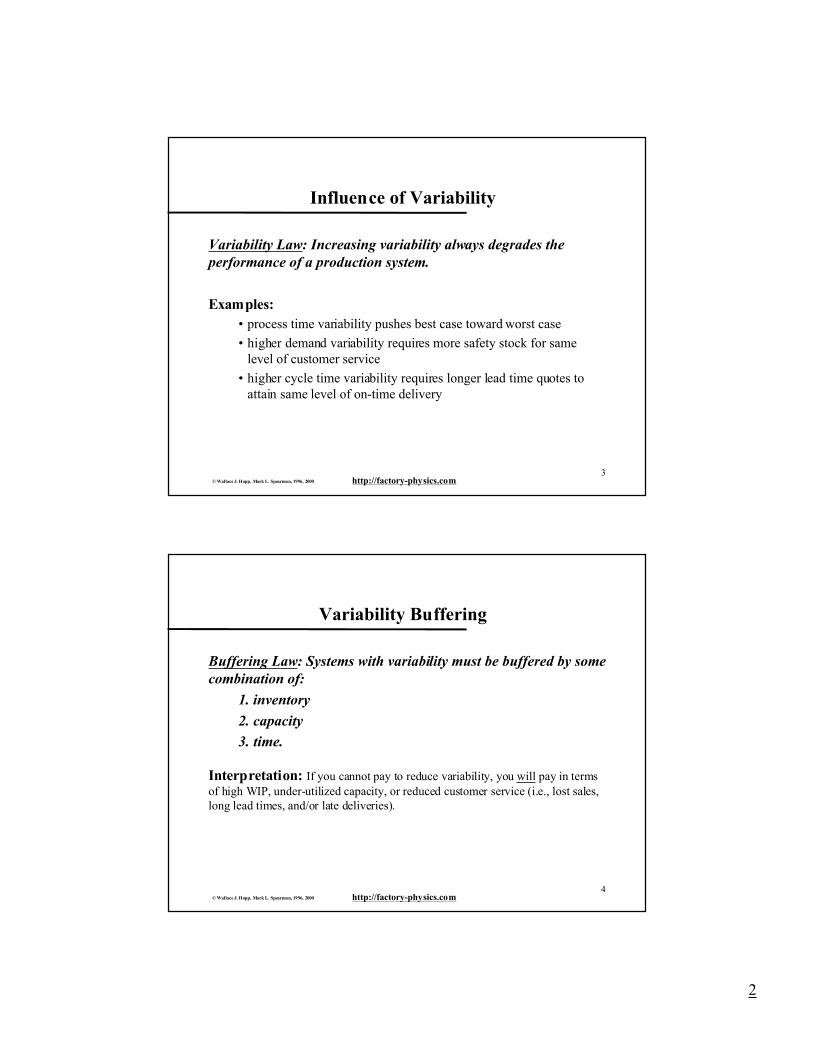
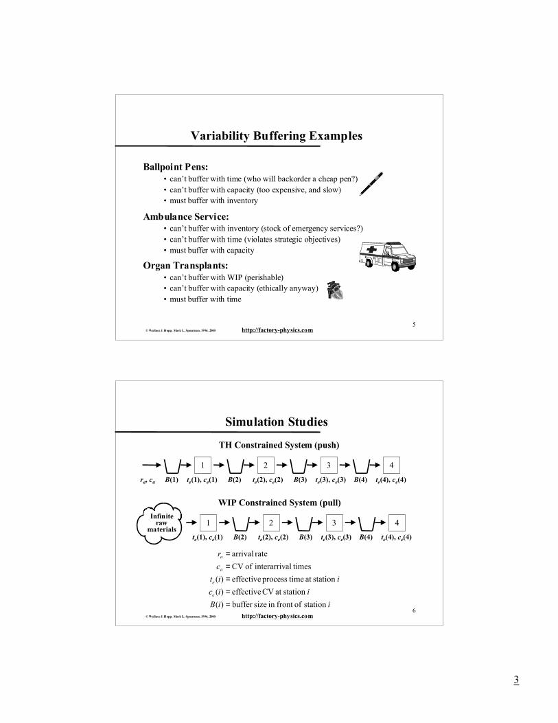
Variability Buffering Examples
Ballpoint Pens:• can’t buffer with time (who will backorder a cheap pen?)• can’t buffer with capacity (too expensive, and slow)• must buffer with inventory
Ambulance Service:• can’t buffer with inventory (stock of emergency services?)• can’t buffer with time (violates strategic objectives)• must buffer with capacity
Organ Transplants:• can’t buffer with WIP (perishable)• can’t buffer with capacity (ethically anyway)• must buffer with time
6© Wallace J. Hopp, Mark L. Spearman, 1996, 2000 http://factory-physics.com
Simulation Studies
1
te(1), ce(1)B(1) te(2), ce(2) te(3), ce(3) te(4), ce(4)B(2) B(4)B(3)ra, ca
2 3 4
TH Constrained System (push)
1
te(1), ce(1) te(2), ce(2) te(3), ce(3) te(4), ce(4)B(2) B(4)B(3)
2 3 4
WIP Constrained System (pull)Infinite
rawmaterials
iiB
iic
iit
c
r
e
e
a
a
station offront in sizebuffer )(
station at CV effective)(
station at timeprocess effective)(
timesalinterarriv of CV
rate arrival
=====
4
7© Wallace J. Hopp, Mark L. Spearman, 1996, 2000 http://factory-physics.com
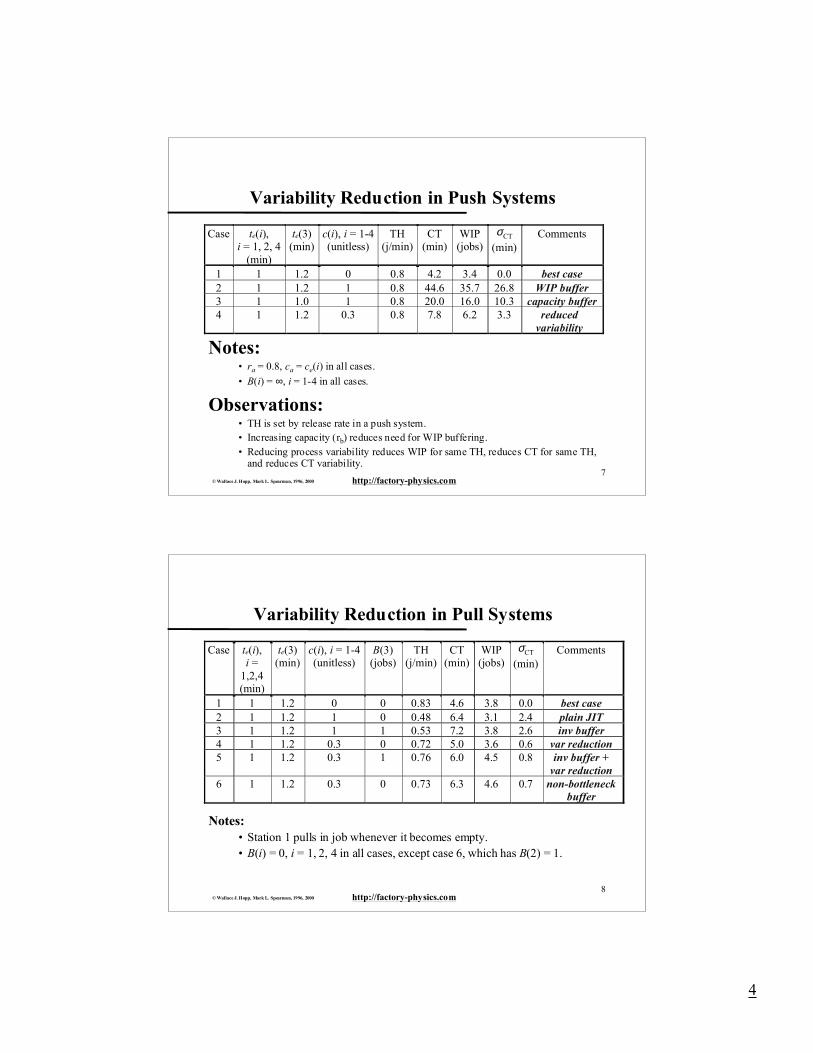
Variability Reduction in Push Systems
Notes:• ra = 0.8, ca = ce(i) in all cases.
• B(i) = ∞, i = 1-4 in all cases.
Observations:• TH is set by release rate in a push system.• Increasing capacity (rb) reduces need for WIP buffering.• Reducing process variability reduces WIP for same TH, reduces CT for same TH,
and reduces CT variability.
Case te(i), i = 1, 2, 4
(min)
te(3) (min)
c(i), i = 1-4 (unitless)
TH (j/min)
CT (min)
WIP (jobs)
σCT (min)
Comments
1 1 1.2 0 0.8 4.2 3.4 0.0 best case 2 1 1.2 1 0.8 44.6 35.7 26.8 WIP buffer 3 1 1.0 1 0.8 20.0 16.0 10.3 capacity buffer 4 1 1.2 0.3 0.8 7.8 6.2 3.3 reduced
variability
8© Wallace J. Hopp, Mark L. Spearman, 1996, 2000 http://factory-physics.com
Variability Reduction in Pull Systems
Notes:• Station 1 pulls in job whenever it becomes empty.• B(i) = 0, i = 1, 2, 4 in all cases, except case 6, which has B(2) = 1.
Case te(i), i =
1,2,4 (min)
te(3) (min)
c(i), i = 1-4 (unitless)
B(3) (jobs)
TH (j/min)
CT (min)
WIP (jobs)
σCT (min)
Comments
1 1 1.2 0 0 0.83 4.6 3.8 0.0 best case 2 1 1.2 1 0 0.48 6.4 3.1 2.4 plain JIT 3 1 1.2 1 1 0.53 7.2 3.8 2.6 inv buffer 4 1 1.2 0.3 0 0.72 5.0 3.6 0.6 var reduction 5 1 1.2 0.3 1 0.76 6.0 4.5 0.8 inv buffer +
var reduction 6 1 1.2 0.3 0 0.73 6.3 4.6 0.7 non-bottleneck
buffer
5
9© Wallace J. Hopp, Mark L. Spearman, 1996, 2000 http://factory-physics.com
Variability Reduction in Pull Systems (cont.)
Observations:• Capping WIP without reducing variability reduces TH.
• WIP cap limits effect of process variability on WIP/CT.
• Reducing process variability increases TH, given same buffers.
• Adding buffer space at bottleneck increases TH.
• Magnitude of impact of adding buffers depends on variability.
• Buffering less helpful at non-bottlenecks.
• Reducing process variability reduces CT variability.
Conclusion: if you can’t pay to reduce variability now, you willpay later with lost throughput, wasted capacity, inflated cycletimes, excess inventory, long lead times,or poor customerservice!
10© Wallace J. Hopp, Mark L. Spearman, 1996, 2000 http://factory-physics.com
Variability from Batching
VUT Equation:• CT depends on process variability and flow variability
Batching:• affects flow variability
• affects waiting inventory
Conclusion: batching is an important determinant of performance
6
11© Wallace J. Hopp, Mark L. Spearman, 1996, 2000 http://factory-physics.com
Process Batch Versus Move Batch
Dedicated Assembly Line: What should the batch size be?
Process Batch:• Related to length of setup.
• The longer the setup the larger the lot size required for the same capacity.
Move (transfer) Batch: Why should it equal process batch?
• The smaller the move batch, the shorter the cycle time.
• The smaller the move batch, the more material handling.
Lot Splitting: Move batch can be different from process batch.
1. Establish smallest economical move batch.2. Group move batches of like families together at bottleneck to avoid setups.3. Implement using a “backlog”.
12© Wallace J. Hopp, Mark L. Spearman, 1996, 2000 http://factory-physics.com
Process Batching Effects
Types of Process Batching:1. Serial Batching:
• processes with sequence-dependent setups
• “batch size” is number of jobs between setups
• batching used to reduce loss of capacity from setups
2. Parallel Batching:
• true “batch” operations (e.g., heat treat)
• “batch size” is number of jobs run together
• batching used to increase effective rate of process
7
13© Wallace J. Hopp, Mark L. Spearman, 1996, 2000 http://factory-physics.com
Process Batching
Process Batching Law: In stations with batch operations orsignificant changeover times:
• The minimum process batch size that yields a stablesystem may be greater than one.
• As process batch size becomes large, cycle time growsproportionally with batch size.
• Cycle time at the station will be minimized for someprocess batch size, which may be greater than one.
Basic Batching Tradeoff: WIP versus capacity
14© Wallace J. Hopp, Mark L. Spearman, 1996, 2000 http://factory-physics.com
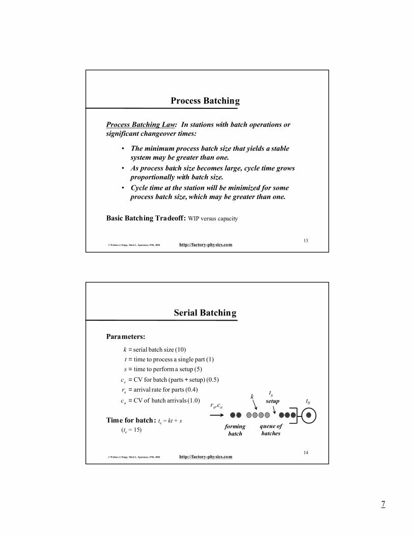
Serial Batching
Parameters:
Time for batch: te = kt + s
(te = 15)
(1.0) arrivalsbatch of CV
(0.4) partsfor rate arrival
(0.5) setup) (partsbatch for CV
(5) setup a perform totime
(1)part single a process totime
(10) sizebatch serial
=
=+=
===
a
a
e
c
r
c
s
t
k
t0
ts
ra,ca
formingbatch
queue ofbatches
setupk
8
15© Wallace J. Hopp, Mark L. Spearman, 1996, 2000 http://factory-physics.com
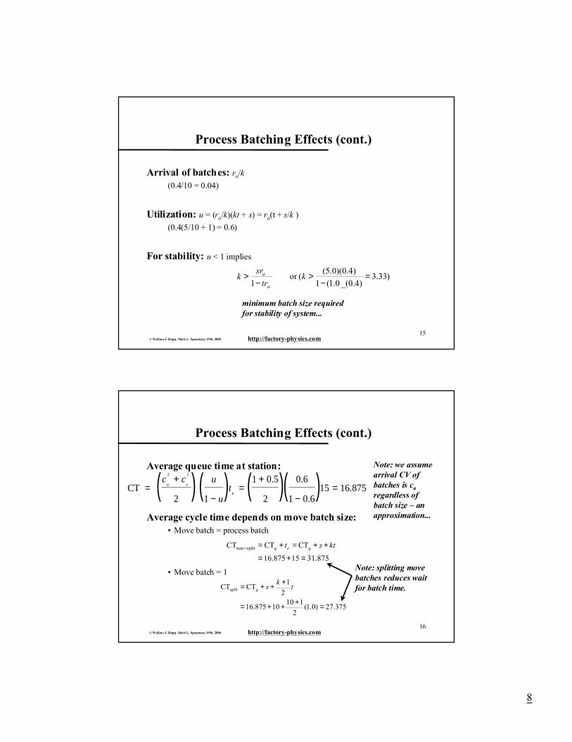
Process Batching Effects (cont.)
Arrival of batches: ra/k
(0.4/10 = 0.04)
Utilization: u = (ra/k)(kt + s) = ra(t + s/k )
(0.4(5/10 + 1) = 0.6)
For stability: u < 1 implies
)33.3)4.0_(0.1(1
)4.0)(0.5((or
1=
−>
−> k
tr
srk
a
a
minimum batch size requiredfor stability of system...
16© Wallace J. Hopp, Mark L. Spearman, 1996, 2000 http://factory-physics.com
Process Batching Effects (cont.)
Average queue time at station:
Average cycle time depends on move batch size:• Move batch = process batch
• Move batch = 1
CT q
c c u
uta e
e=
+
−=
+
−=( ) ( ) ( )( )2 2
2 1
1 0 5
2
0 6
1 0 615 16 875
. .
..
875.3115875.16
CTCTCT splitnon
=+=
++=+=− ktst qeq
375.27)0.1(2
11010875.16
2
1CTCTsplit
=+++=
+++= tk
sq
Note: splitting movebatches reduces waitfor batch time.
Note: we assumearrival CV of batches is ca regardless of batch size – anapproximation...
9
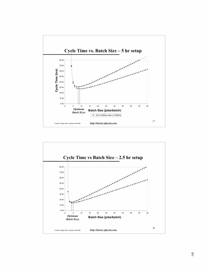
17© Wallace J. Hopp, Mark L. Spearman, 1996, 2000 http://factory-physics.com
Cycle Time vs. Batch Size – 5 hr setup
0.00
10.00
20.00
30.00
40.00
50.00
60.00
70.00
80.00
0 5 10 15 20 25 30 35 40 45 50
Batch Size (jobs/batch)
Cyc
le T
ime
(hrs
)
No Lot Splitting Lot Splitting
OptimumBatch Sizes
18© Wallace J. Hopp, Mark L. Spearman, 1996, 2000 http://factory-physics.com
Cycle Time vs Batch Size – 2.5 hr setup
0.00
10.00
20.00
30.00
40.00
50.00
60.00
70.00
80.00
0 5 10 15 20 25 30 35 40 45 50
Batch Size (jobs/batch)OptimumBatch Sizes
10
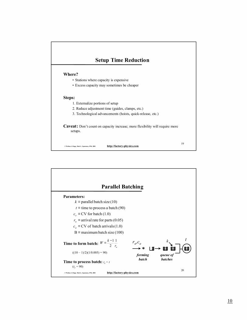
19© Wallace J. Hopp, Mark L. Spearman, 1996, 2000 http://factory-physics.com
Setup Time Reduction
Where?• Stations where capacity is expensive
• Excess capacity may sometimes be cheaper
Steps:1. Externalize portions of setup
2. Reduce adjustment time (guides, clamps, etc.)
3. Technological advancements (hoists, quick-release, etc.)
Caveat: Don’t count on capacity increase; more flexibility will require moresetups.
20© Wallace J. Hopp, Mark L. Spearman, 1996, 2000 http://factory-physics.com
Parallel Batching
Parameters:
Time to form batch:
((10 – 1)/2)(1/0.005) = 90)
Time to process batch: te = t(te = 90)
(100) sizebatch maximumB
(1.0) arrivalsbatch of CV
(0.05) partsfor rate arrival
(1.0)batch for CV
(90)batch a process totime
(10) sizebatch parallel
======
a
a
e
c
r
c
t
k
ar
kW
1
2
1−=tra,ca
formingbatch
queue ofbatches
k
11
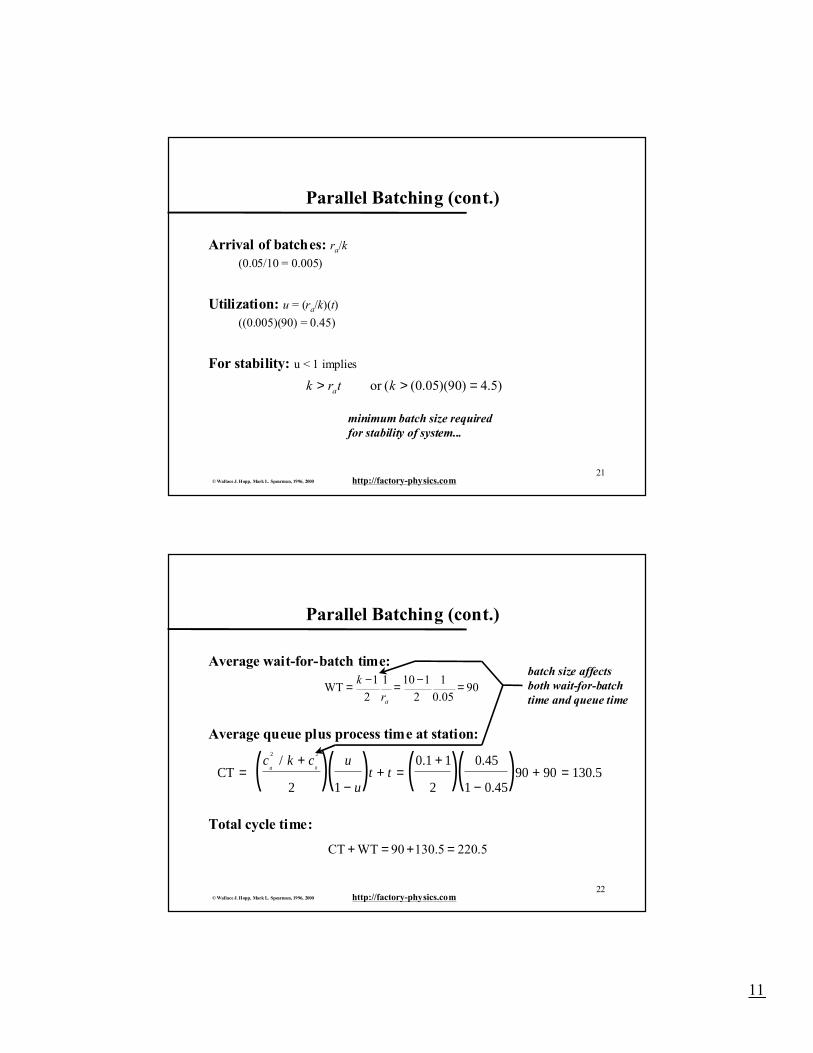
21© Wallace J. Hopp, Mark L. Spearman, 1996, 2000 http://factory-physics.com
Parallel Batching (cont.)
Arrival of batches: ra/k
(0.05/10 = 0.005)
Utilization: u = (ra/k)(t)
((0.005)(90) = 0.45)
For stability: u < 1 implies
)5.4)90)(05.0((or =>> ktrk a
minimum batch size requiredfor stability of system...
22© Wallace J. Hopp, Mark L. Spearman, 1996, 2000 http://factory-physics.com
Parallel Batching (cont.)
Average wait-for-batch time:
Average queue plus process time at station:
Total cycle time:
CT =+
−+ =
+
−+ =( )( ) ( )( )c k c u
ut ta
2
0
2
2 1
0 1 1
2
0 45
1 0 4590 90 130 5
/ . .
..
5.2205.13090WTCT =+=+
9005.0
1
2
1101
2
1WT =−=−=
ar
kbatch size affects both wait-for-batch time and queue time
12
23© Wallace J. Hopp, Mark L. Spearman, 1996, 2000 http://factory-physics.com
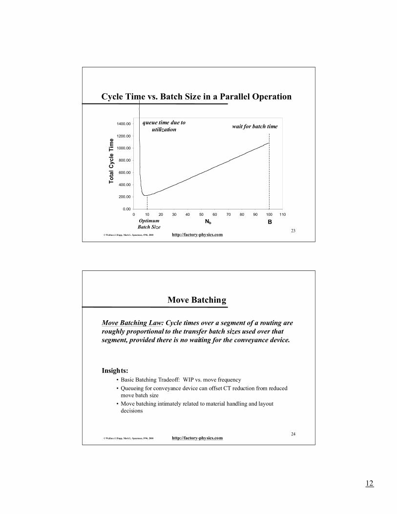
Cycle Time vs. Batch Size in a Parallel Operation
0.00
200.00
400.00
600.00
800.00
1000.00
1200.00
1400.00
0 10 20 30 40 50 60 70 80 90 100 110
Nb
To
tal
Cyc
le T
ime
queue time due toutilization wait for batch time
BOptimumBatch Size
24© Wallace J. Hopp, Mark L. Spearman, 1996, 2000 http://factory-physics.com
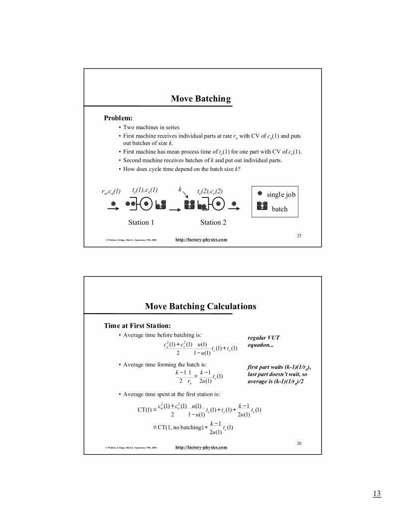
Move Batching
Move Batching Law: Cycle times over a segment of a routing areroughly proportional to the transfer batch sizes used over thatsegment, provided there is no waiting for the conveyance device.
Insights:• Basic Batching Tradeoff: WIP vs. move frequency
• Queueing for conveyance device can offset CT reduction from reducedmove batch size
• Move batching intimately related to material handling and layoutdecisions
13
25© Wallace J. Hopp, Mark L. Spearman, 1996, 2000 http://factory-physics.com
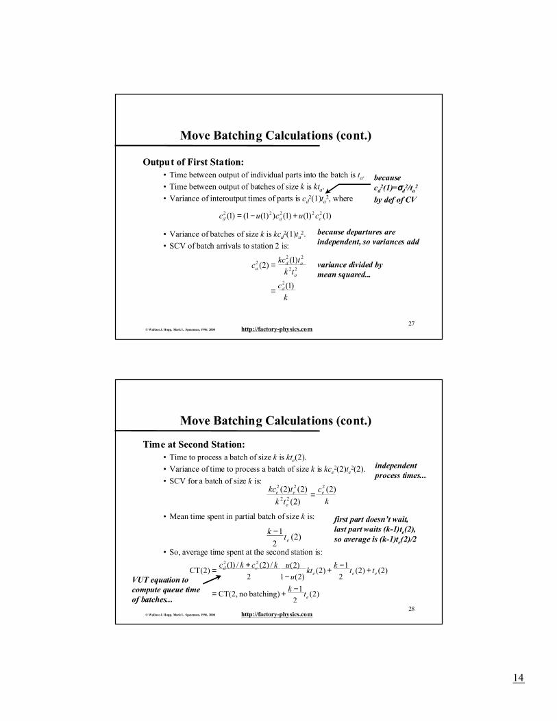
Move Batching
Problem:• Two machines in series
• First machine receives individual parts at rate ra with CV of ca(1) and putsout batches of size k.
• First machine has mean process time of te(1) for one part with CV of ce(1).
• Second machine receives batches of k and put out individual parts.
• How does cycle time depend on the batch size k?
batch
single job
Station 1 Station 2
kra,ca(1) te(1),ce(1) te(2),ce(2)
26© Wallace J. Hopp, Mark L. Spearman, 1996, 2000 http://factory-physics.com
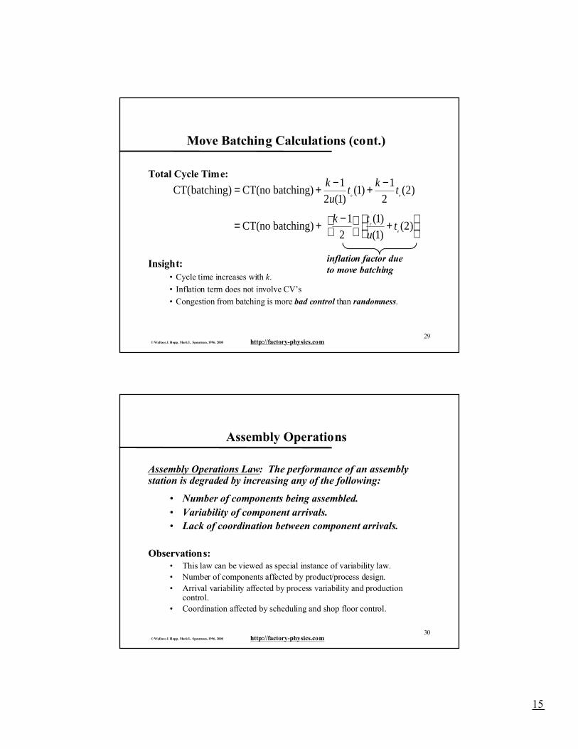
Move Batching Calculations
Time at First Station:• Average time before batching is:
• Average time forming the batch is:
• Average time spent at the first station is:
)1()1()1(1
)1(
2
)1()1( 22
eeea tt
u
ucc +−
+
)1()1(2
112
1e
a
tu
kr
k −=−
)1()1(2
1)batching no CT(1,
)1()1(2
1)1()1(
)1(1
)1(
2
)1()1()1(CT
22
e
eeeea
tu
k
tu
ktt
u
ucc
−+=
−++−
+=
regular VUTequation...
first part waits (k-1)(1/ra),last part doesn’t wait, so average is (k-1)(1/ra)/2
14
27© Wallace J. Hopp, Mark L. Spearman, 1996, 2000 http://factory-physics.com
Move Batching Calculations (cont.)
Output of First Station:• Time between output of individual parts into the batch is ta.
• Time between output of batches of size k is kta.
• Variance of interoutput times of parts is cd2(1)ta2, where
• Variance of batches of size k is kcd2(1)ta
2.
• SCV of batch arrivals to station 2 is:
)1()1()1())1(1()1( 22222ead cucuc +−=
k
c
tk
tkcc
d
a
ada
)1(
)1()2(
2
22
222
=
=
becausecd
2(1)=σσσσd2/ta2
by def of CV
because departures are independent, so variances add
variance divided by mean squared...
28© Wallace J. Hopp, Mark L. Spearman, 1996, 2000 http://factory-physics.com
Move Batching Calculations (cont.)
Time at Second Station:• Time to process a batch of size k is kte(2).
• Variance of time to process a batch of size k is kce2(2)te2(2).
• SCV for a batch of size k is:
• Mean time spent in partial batch of size k is:
• So, average time spent at the second station is:
k
c
tk
tkc e
e
ee )2(
)2(
)2()2( 2
22
22
=
)2(2
1et
k −
)2(2
1)batching no CT(2,
)2()2(2
1)2(
)2(1
)2(
2
/)2(/)1()2(CT
22
e
eeeed
tk
ttk
ktu
ukckc
−+=
+−+−
+=
independentprocess times...
first part doesn’t wait,last part waits (k-1)te(2),so average is (k-1)te(2)/2
VUT equation tocompute queue timeof batches...
15
29© Wallace J. Hopp, Mark L. Spearman, 1996, 2000 http://factory-physics.com
Move Batching Calculations (cont.)
Total Cycle Time:
Insight:• Cycle time increases with k.
• Inflation term does not involve CV’s
• Congestion from batching is more bad control than randomness.
CT batching CT(no batching)
CT(no batching
( )( )
( ) ( )
)( )( )
( )
= + − + −
= + −
+
k
ut
kt
k t
ut
e e
e
e
12 1
11
22
12
11
2
inflation factor dueto move batching
30© Wallace J. Hopp, Mark L. Spearman, 1996, 2000 http://factory-physics.com
Assembly Operations
Assembly Operations Law: The performance of an assemblystation is degraded by increasing any of the following:
• Number of components being assembled.• Variability of component arrivals.• Lack of coordination between component arrivals.
Observations:• This law can be viewed as special instance of variability law.• Number of components affected by product/process design.• Arrival variability affected by process variability and production
control.• Coordination affected by scheduling and shop floor control.
16
31© Wallace J. Hopp, Mark L. Spearman, 1996, 2000 http://factory-physics.com
Attacking Variability
Objectives• reduce cycle time
• increase throughput
• improve customer service
Levers• reduce variability directly
• buffer using inventory
• buffer using capacity
• buffer using time
32© Wallace J. Hopp, Mark L. Spearman, 1996, 2000 http://factory-physics.com
Cycle Time
Definition (Station Cycle Time): The average cycle timeat a station is made up of the following components
cycle time = move time + queue time + setup time + process time + wait-to-batch time + wait-in-batch time + wait-to-match time
Definition (Line Cycle Time): The average cycle time in a line isequal to the sum of the cycle times at the individual stations lessany time that overlaps two or more stations.
delay timestypicallymake up90% of CT
17
33© Wallace J. Hopp, Mark L. Spearman, 1996, 2000 http://factory-physics.com
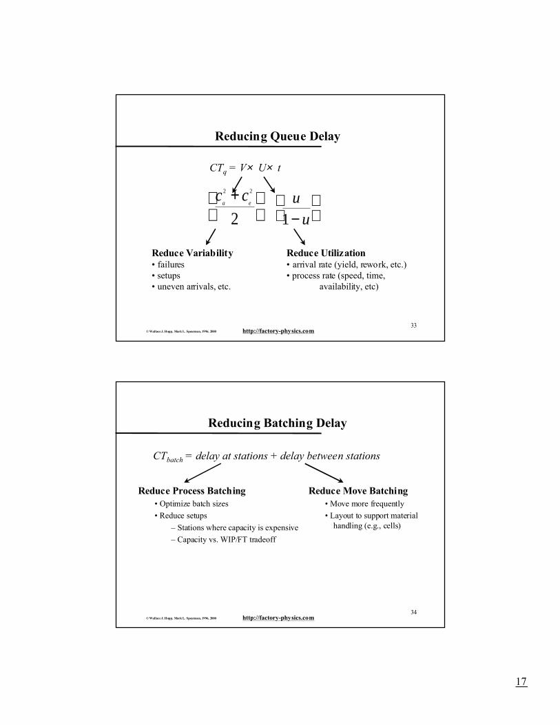
Reducing Queue Delay
CTq = V× U× t
c c
a e
2 2
2+
u
u1−
Reduce Variability • failures• setups• uneven arrivals, etc.
Reduce Utilization• arrival rate (yield, rework, etc.)• process rate (speed, time,
availability, etc)
34© Wallace J. Hopp, Mark L. Spearman, 1996, 2000 http://factory-physics.com
Reducing Batching Delay
Reduce Process Batching• Optimize batch sizes
• Reduce setups
– Stations where capacity is expensive
– Capacity vs. WIP/FT tradeoff
Reduce Move Batching• Move more frequently
• Layout to support material handling (e.g., cells)
CTbatch = delay at stations + delay between stations
18
35© Wallace J. Hopp, Mark L. Spearman, 1996, 2000 http://factory-physics.com
Reducing Matching Delay
Improve Coordination• scheduling
• pull mechanisms
• modular designs
Reduce Variability• High utilization fabrication lines
• Usual variability reduction methods
CTbatch = delay due to lack of synchronization
Reduce Number of Components
• product redesign
• kitting
36© Wallace J. Hopp, Mark L. Spearman, 1996, 2000 http://factory-physics.com
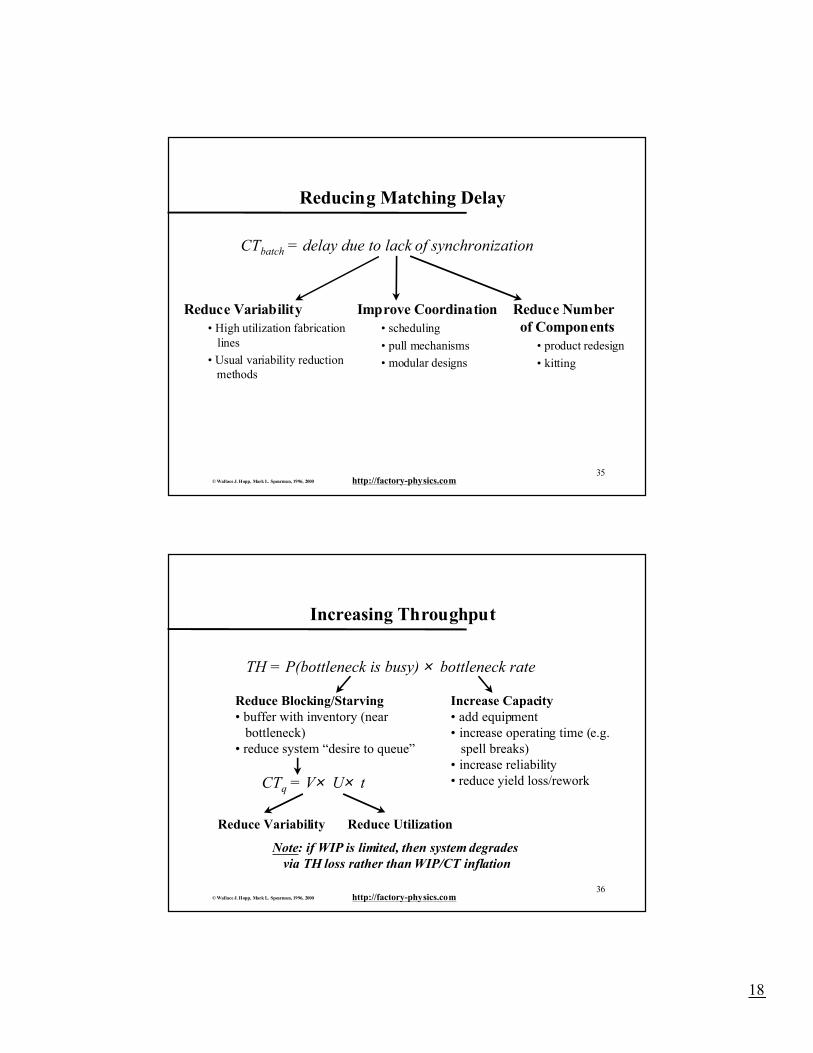
Increasing Throughput
TH = P(bottleneck is busy) × bottleneck rate
Increase Capacity• add equipment• increase operating time (e.g. spell breaks)• increase reliability• reduce yield loss/rework
Reduce Blocking/Starving• buffer with inventory (near bottleneck)• reduce system “desire to queue”
CTq = V× U× t
Reduce Variability Reduce Utilization
Note: if WIP is limited, then system degrades via TH loss rather than WIP/CT inflation
19
37© Wallace J. Hopp, Mark L. Spearman, 1996, 2000 http://factory-physics.com
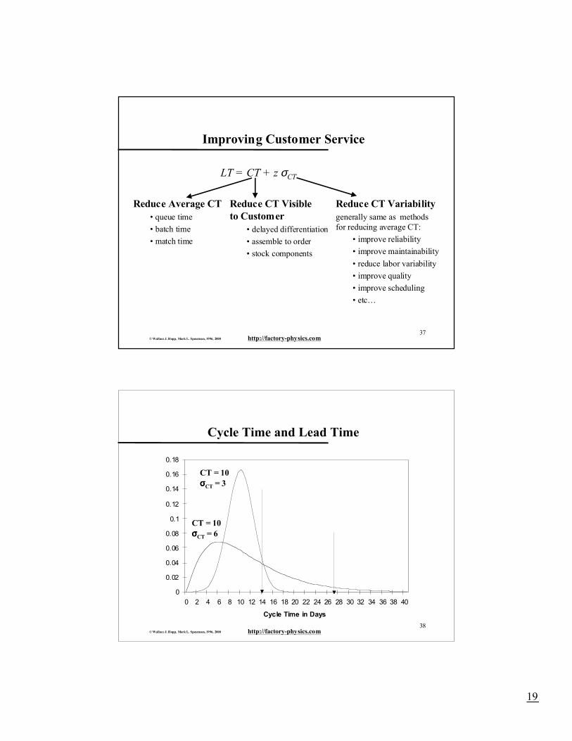
Improving Customer Service
LT = CT + z σCT
Reduce Average CT• queue time
• batch time
• match time
Reduce CT Variabilitygenerally same as methods for reducing average CT:
• improve reliability
• improve maintainability
• reduce labor variability
• improve quality
• improve scheduling
• etc…
Reduce CT Visibleto Customer
• delayed differentiation
• assemble to order
• stock components
38© Wallace J. Hopp, Mark L. Spearman, 1996, 2000 http://factory-physics.com
Cycle Time and Lead Time
0
0.02
0.04
0.06
0.08
0.1
0.12
0.14
0.16
0.18
0 2 4 6 8 10 12 14 16 18 20 22 24 26 28 30 32 34 36 38 40
Cycle Time in Days
CT = 10σσσσCT = 3
CT = 10σσσσCT = 6
20
39© Wallace J. Hopp, Mark L. Spearman, 1996, 2000 http://factory-physics.com
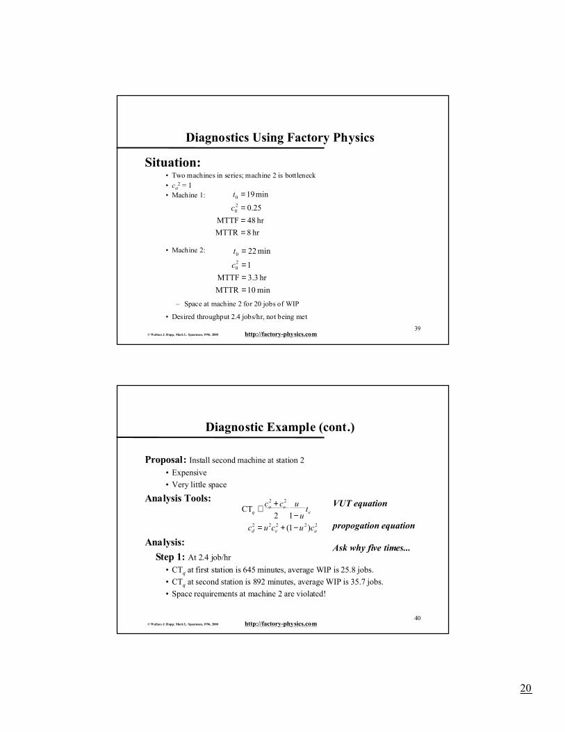
Diagnostics Using Factory Physics
Situation:• Two machines in series; machine 2 is bottleneck• ca
2 = 1• Machine 1:
• Machine 2:
– Space at machine 2 for 20 jobs of WIP
• Desired throughput 2.4 jobs/hr, not being met
hr 8MTTR
hr 48MTTF
25.0
min1920
0
===
=
c
t
min 10MTTR
hr 3.3MTTF
1
min2220
0
===
=
c
t
40© Wallace J. Hopp, Mark L. Spearman, 1996, 2000 http://factory-physics.com
Diagnostic Example (cont.)
Proposal: Install second machine at station 2
• Expensive
• Very little space
Analysis Tools:
Analysis:
Step 1: At 2.4 job/hr
• CTq at first station is 645 minutes, average WIP is 25.8 jobs.
• CTq at second station is 892 minutes, average WIP is 35.7 jobs.
• Space requirements at machine 2 are violated!
22222
22
)1(12
CT
aed
eea
q
cucuc
tu
ucc
−+=−
+∪ VUT equation
propogation equation
Ask why five times...
21
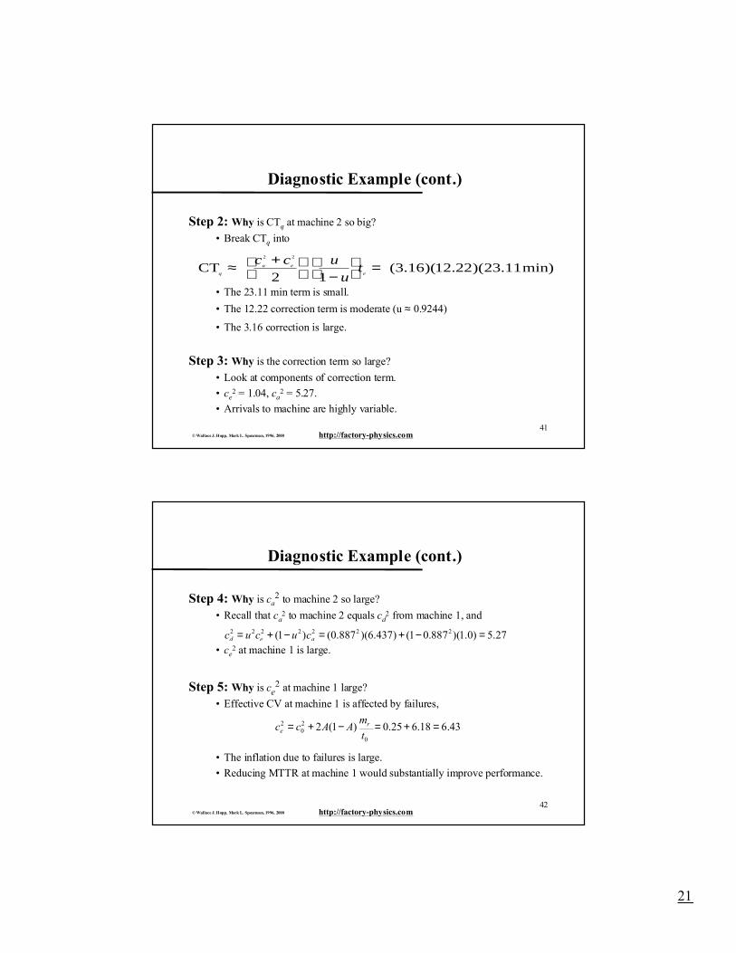
41© Wallace J. Hopp, Mark L. Spearman, 1996, 2000 http://factory-physics.com
Diagnostic Example (cont.)
Step 2: Why is CTq at machine 2 so big?
• Break CTq into
• The 23.11 min term is small.
• The 12.22 correction term is moderate (u ≈ 0.9244)
• The 3.16 correction is large.
Step 3: Why is the correction term so large?
• Look at components of correction term.
• ce2 = 1.04, ca
2 = 5.27.
• Arrivals to machine are highly variable.
CT q
a e
e
c c u
ut≈ +
−
=
2 2
2 13 16 12 22 23 11( . )( . )( . min)
42© Wallace J. Hopp, Mark L. Spearman, 1996, 2000 http://factory-physics.com
Diagnostic Example (cont.)
Step 4: Why is ca2 to machine 2 so large?
• Recall that ca2 to machine 2 equals cd
2 from machine 1, and
• ce2 at machine 1 is large.
Step 5: Why is ce2 at machine 1 large?
• Effective CV at machine 1 is affected by failures,
• The inflation due to failures is large.
• Reducing MTTR at machine 1 would substantially improve performance.
27.5)0.1)(887.01()437.6)(887.0()1( 2222222 =−+=−+= aed cucuc
43.618.625.0)1(20
20
2 =+=−+=t
mAAcc r
e
22
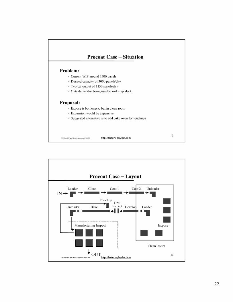
43© Wallace J. Hopp, Mark L. Spearman, 1996, 2000 http://factory-physics.com
Procoat Case – Situation
Problem:• Current WIP around 1500 panels
• Desired capacity of 3000 panels/day
• Typical output of 1150 panels/day
• Outside vendor being used to make up slack
Proposal:• Expose is bottleneck, but in clean room
• Expansion would be expensive
• Suggested alternative is to add bake oven for touchups
44© Wallace J. Hopp, Mark L. Spearman, 1996, 2000 http://factory-physics.com
Procoat Case – Layout
Loader
BakeUnloader
UnloaderCoat 1Clean
D&IInspect
Touchup
Manufacturing Inspect
Loader
Expose
Clean Room
Coat 2
Develop
IN
OUT
23
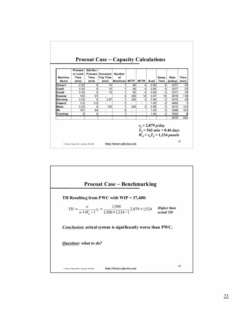
45© Wallace J. Hopp, Mark L. Spearman, 1996, 2000 http://factory-physics.com
Procoat Case – Capacity Calculations
Machine Name
Process or Load
Time (min)
Std Dev Process
Time (min)
Conveyor Trip Time
(min)
Number of
Machines MTTF MTTR AvailSetup Time
Rate (p/day)
Time (min)
Clean1 0.33 0 15 1 80 4 0.95 0 3377 37Coat1 0.33 0 15 1 80 4 0.95 0 3377 37Coat2 0.33 0 15 1 80 4 0.95 0 3377 37Expose 103 67 - 5 300 10 0.97 15 2879 118Develop 0.33 0 2.67 1 300 3 0.99 0 3510 23Inspect 0.5 0.5 - 2 - - 1.00 0 4680 1Bake 0.33 0 100 1 300 3 0.99 0 3510 121MI 161 64 - 8 - - 1.00 0 3488 161Touchup 9 0 - 1 - - 1.00 0 7800 9
2879 542
rb = 2,879 p/dayT0 = 542 min = 0.46 daysW0 = rbT0 = 1,334 panels
46© Wallace J. Hopp, Mark L. Spearman, 1996, 2000 http://factory-physics.com
Procoat Case – Benchmarking
TH Resulting from PWC with WIP = 37,400:
Conclusion: actual system is significantly worse than PWC.
524,1879,21334,1500,1
500,110
=−+
=−+
= brWww
TH Higher than actual TH
Question: what to do?
24
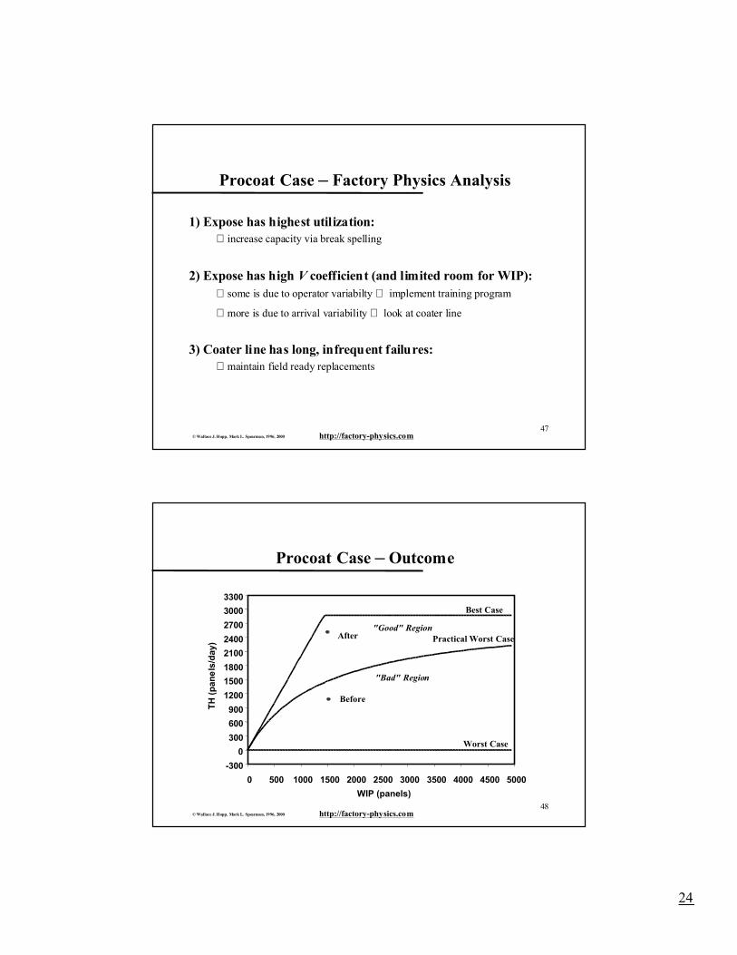
47© Wallace J. Hopp, Mark L. Spearman, 1996, 2000 http://factory-physics.com
Procoat Case – Factory Physics Analysis
1) Expose has highest utilization:⇒ increase capacity via break spelling
2) Expose has high V coefficient (and limited room for WIP):⇒ some is due to operator variabilty ⇒ implement training program
⇒ more is due to arrival variability ⇒ look at coater line
3) Coater line has long, infrequent failures:⇒ maintain field ready replacements
48© Wallace J. Hopp, Mark L. Spearman, 1996, 2000 http://factory-physics.com
Procoat Case – Outcome
-300
0
300
600
900
1200
1500
1800
2100
2400
2700
3000
3300
0 500 1000 1500 2000 2500 3000 3500 4000 4500 5000
WIP (panels)
TH
(p
ane
ls/d
ay)
Best Case
Practical Worst Case
Worst Case
Before
"Good" Region
"Bad" Region
After
25
49© Wallace J. Hopp, Mark L. Spearman, 1996, 2000 http://factory-physics.com
Corrupting Influence Takeaways
Variance Causes Congestion:• many sources of variability
• planned and unplanned
Variability and Utilization Interact:• congestion effects multiply
• utilization effects are highly nonlinear
• importance of bottleneck management
50© Wallace J. Hopp, Mark L. Spearman, 1996, 2000 http://factory-physics.com
Corrupting Influence Takeaways (cont.)
Variability Propagates:• flow variability is as disruptive as process variability
• non-bottlenecks can be major problems
Variability Must be Buffered:• inventory
• capacity
• time