Embed Size (px)
Citation preview
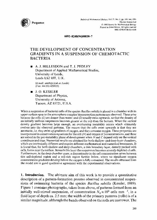
Perg,mo. Bulletin of Mathematical Biology, Vol. 57, No. 2, pp. 299 344, 1995
Elsevier Science Ltd �9 1995 Society for Mathematical Biology
Printed in Great Britain. All rights reserved 0092-8240/95 $9.50 + 0.00
0092-8240(94)00038-7
T H E D E V E L O P M E N T O F C O N C E N T R A T I O N G R A D I E N T S I N A S U S P E N S I O N O F C H E M O T A C T I C B A C T E R I A
�9 A .J . H I L L E S D O N and T. J. PEDLEY Department of Applied Mathematical Studies, University of Leeds, Leeds LS2 9JT, U.K.
(E.mail: [email protected]) (Fax: 44-532-429925)
�9 J .O . KESSLER Department of Physics, University of Arizona, Tucson, AZ 85721, U.S.A.
When a suspension of bacterial cells of the species Bacillus subtilis is placed in a chamber with its upper surface open to the atmosphere complex bioconvection patterns are observed. These arise because the cells: (1) are denser than water; and (2) usually swim upwards, so that the density of an initially uniform suspension becomes greater at the top than the bottom. When the vertical density gradient becomes large enough, an overturning instability occurs which ultimately evolves into the observed patterns. The reason that the cells swim upwards is that they are aerotactic, i.e. they swim up gradients of oxygen, and they consume oxygen. These properties are incorporated in conservation equations for the cell (N) and oxygen (C) concentrations, and these are solved in the pre-instability phase of development when N and C depend only on the vertical coordinate and time. Numerical results are obtained for both shallow- and deep-layer chambers, which are intrinsically different and require different mathematical and numerical treatments. It is found that, for both shallow and deep chambers, a thin boundary layer, densely packed with cells, forms near the surface. Beneath this layer the suspension becomes severely depleted of cells. Furthermore, in the deep chamber cases, a discontinuity in the cell concentration arises between this cell-depleted region and a cell-rich region further below, where no significant oxygen concentration gradients develop before the oxygen is fully consumed. The results obtained from the model are in good qualitative agreement with the experimental observations.
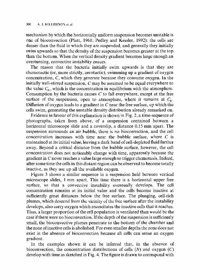
1. Introduction. The ultimate aim of this work is to provide a quantitative description of a pattern-formation process observed in concentrated suspen- sions of swimming bacteria of the species Bacillus subtilis (Kessler, 1989). Figure 1 contains photographs, taken from above, of patterns formed from an initially well-stirred suspension, of concentration No~ 10 6 cells mm -3, in a fluid layer of depth ca. 2.5 mm; the width of the primary patterns (rolls) is of a similar magnitude, although the bands observed on the rolls are narrower. The
299
300 A.J. HILLESDON et al.
mechanism by which the horizontally uniform suspension becomes unstable is one of bioconvection (Platt, 1961; Pedley and Kessler, 1992): the cells are denser than the fluid in which they are suspended, and generally they initially swim upwards so that the density of the suspension becomes greater at the top than the bottom. When the vertical density gradient becomes large enough an overturning, convective instability ensues.
The reason that the bacteria initially swim upwards is that they are chemotactic (or, more strictly, aerotactic), swimming up a gradient of oxygen concentration, C, which they generate because they consume oxygen. In the initially well-stirred suspension, C may be assumed to be equal everywhere to the value Co, which is the concentration in equilibrium with the atmosphere. Consumption by the bacteria causes C to fall everywhere, except at the free surface of the suspension, open to atmosphere, where it remains at Co. Diffusion of oxygen leads to a gradient in C near the free surface, up which the cells swim, generating the unstable density distribution already remarked on.
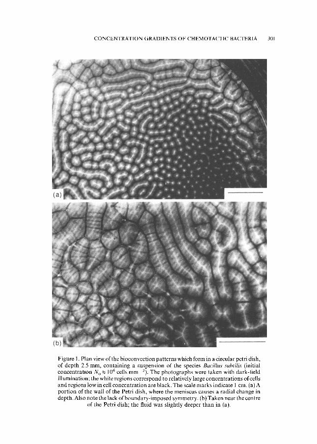
Evidence in favour of this explanation is shown in Fig. 2, a time-sequence of photographs, taken from above, of a suspension contained between a horizontal microscope slide and a coverslip, a distance 0.15 mm apart. The suspension surrounds an air bubble, there is no bioconvection, and the cell concentration increases with time near the bubble surface, where C is maintained at its initial value, leaving a dark band of cell-depleted fluid further away. Beyond a critical distance from the bubble surface, however, the cell concentration does not noticeably change with time, apparently because the gradient in C never reaches a value large enough to trigger chemotaxis. Indeed, after some time the cells in this distant region can be observed to become totally inactive, as they use up all the available oxygen.
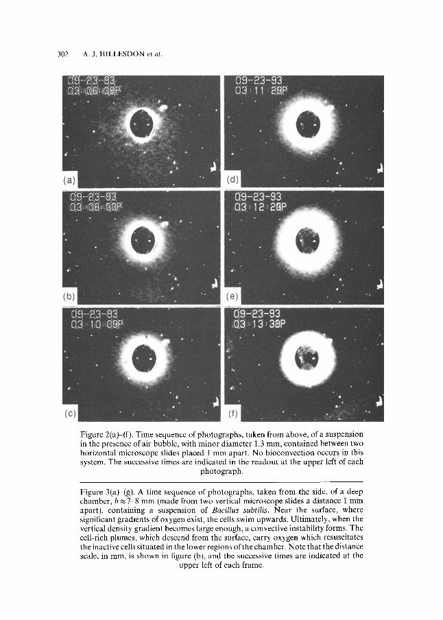
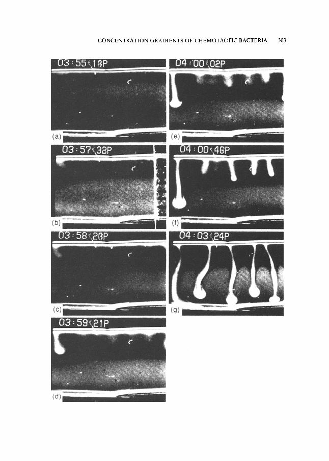
Figure 3 shows a similar sequence in a suspension held between vertical microscope slides, 1 mm apart. This time there is a horizontal upper free surface, so that a convective instability eventually develops. The cell concentration remains at its initial value and the cells become inactive at sufficiently great distances below the free surface. The plunging, cell-rich plumes, which descend from the vicinity of the free surface after the instability develops, also carry oxygen which resuscitates the inactive cells that it reaches. Thus, a larger proportion of the cell population is ventilated than would be the case if there were no bioconvection. If the depth of the suspension is sufficiently small, the bioconvective plumes penetrate to the bot tom of the chamber and the zone of inactive cells is abolished. For even smaller depths the zone does not exist in the absence of bioconvection because all cells can sense an oxygen gradient.
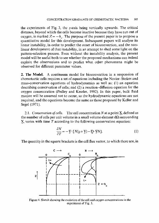
In the examples shown it can be inferred that, in the absence of bioconvection, the concentration distributions of cells (N) and oxygen (C) develop with time as sketched in Fig. 4. The figure is drawn to correspond with
CONCENTRATION GRADIENTS OF CHEMOTACTIC BACTERIA 301
Figure 1. Plan view of the bioconvection patterns which form in a circular petri dish, of depth 2.5 ram, containing a suspension of the species Bacillus subtilis (initial concentration N o ~ 10 6 cells mm 3). The photographs were taken with dark-field illumination; the white regions correspond to relatively large concentrations of cells and regions low in cell concentration are black. The scale marks indicate i cm. (a) A portion of the wall of the Petri dish, where the meniscus causes a radial change in depth. Also note the lack of boundary-imposed symmetry. (b) Taken near the centre
of the Petri dish; the fluid was slightly deeper than in (a).
302 A.J. HILLESDON et al.
Figure 2(a)-(f). Time sequence of photographs, taken from above, of a suspension in the presence of air bubble, with minor diameter 1.3 mm, contained between two horizontal microscope slides placed 1 mm apart. No bioconvection occurs in this system. The successive times are indicated in the readout at the upper left of each
photograph.
Figure 3(a)-(g). A time sequence of photographs, taken from the side, of a deep chamber, h ~ 7-8 mm (made from two vertical microscope slides a distance 1 mm apart), containing a suspension of Bacillus subtilis. Near the surface, where significant gradients of oxygen exist, the cells swim upwards. Ultimately, when the vertical density gradient becomes large enough, a convective instability forms. The cell-rich plumes, which descend from the surface, carry oxygen which resuscitates the inactive cells situated in the lower regions of the chamber. Note that the distance scale, in ram, is shown in figure (b), and the successive times are indicated at the
upper left of each frame.
CONCENTRATION GRADIENTS OF CHEMOTACTIC BACTERIA 303

CONCENTRATION GRADIENTS OF CHEMOTACTIC BACTERIA 305
the experiments of Fig. 3, the z-axis being vertically upwards. The critical distance, beyond which the cells become inactive because they have run out of oxygen, is marked Z = - h c. The purpose of the present paper is to propose a quantitative model for this development. Subsequent papers will analyse its linear instability, in order to predict the onset of bioconvection, and the non- linear development of that instability, in an attempt to shed some light on the pattern-selection process. Even without the instability analysis, the present model will be useful both to see whether the proposed mechanisms can indeed explain the observations and to predict what other phenomena might be observed for different parameter values.
2. The Model. A continuum model for bioconvection in a suspension of chemotactic cells requires a set of equations including the Navier-Stokes and mass-conservation equations of hydrodynamics as well as: (1) an equation describing conservation of cells; and (2) a reaction-diffusion equation for the oxygen concentration (Pedley and Kessler, 1992). In this paper, bulk fluid motion will be assumed not to occur, so the hydrodynamic equations are not required, and the equations become the same as those proposed by Keller and Segel (1971).
2.1. Conservation of cells. The cell concentration N at a point X, defined as the number of cells per unit volume in a small volume element df~ surrounding X, varies with time T according to the following conservation equation:
~N ~ T - -V" [N('v+ -V)- D" ~N]" (1)
The quantity in the square brackets is the cell flux vector, to which there are, in
zl
C -----9
0 C 0
N
0 N O
I ~ . r ,
I
J I I I I t+
--J- ..... Z =-h
l i i
Figure 4. Sketch showing the evolution of the cell and oxygen concentrations in the experiment of Fig. 3.
306 A.J. HILLESDON e t al.
general, three contributions. The first term, N u, represents advection by the bulk fluid velocity N which is taken to be zero here. The second term, NV, represents the flux due to directed cell swimming: V is the average swimming velocity of the cells in the volume element df~, and arises in the present example from chemotaxis. The third term in the cell flux represents diffusion of cells (D is the cell diffusivity tensor) and arises from the fact that individual cells swim actively all the time, but in random directions, as long as there is enough oxygen available; this process is termed chemokinesis (Keller et al., 1977). There could, in principle, also be a contribution to cell movement, and hence to D, from Brownian motion, and a contribution to V from sedimentation. The sedimentation speed in water of a sphere of diameter 2 #m, with density 1.1 times that of water, is ca. 0.2 #m sec-1,100 times less than the maximum cell swimming speed. Similarly, a typical Brownian diffusivity for particles of such a size is 5 x 10- 9 cm 2 sec- t, much smaller than a typical cell diffusivity tensor ( ~ l . 3 x l 0 - 6 c m Z s e c - X for a (long) run time, r, of ca. lsec). Thus, sedimentation and Brownian diffusion are negligible, except possibly in a region where the cells have become inactive, and henceforth they are neglected. Equation (1) does not contain a term representing biological growth or decay of the bacterial population because the time-scale for pattern development, of order 1 min, is much smaller than the reproductive time-scale of several hours.
A self-consistent model for the quantities V and D would include both random and deterministic aspects of cell motion in a probability density function for the cell swimming direction (Pedley and Kessler, 1990). Insufficient knowledge of cell behaviour precludes this type of approach at present. Observations show that cells swim at a speed V s of several #m sec-1, and change direction randomly on a time scale, ~, of a fraction of a second. These quantities depend on C but are otherwise presumed to be an intrinsic property of the cells.
If C is large enough, and uniform, the distribution function of cell swimming direction is isotropic, and so, therefore, is the cell diffusivity tensor D. Its magnitude, D N, will, following the standard argument from kinetic theory, be equal to �89 where 2 is the "mean free path" or average distance between direction changes (Berg, 1983). This is the same as:
DN=�89 (2)
If C is not uniform chemotaxis takes place. This is believed to be because the time v between direction changes increases if the ambient oxygen concentration is increasing with time, i.e. if the cell is swimming up a concentration gradient, and decreases if the ambient oxygen concentration is decreasing (Berg, 1975; Schnitzer et al., 1990).
The cell swimming speed V s has an approximately constant value V~0
CONCENTRATION GRADIENTS OF CHEMOTACTIC BACTERIA 307
20 #m sec- 1 if there is enough oxygen available. However, the cell becomes completely inactive if the ambient value of C falls below some small positive value Cmi . (see Appendix A). It is therefore reasonable to suppose that we can write, as a model for the cell swimming speed as a function of oxygen concentrat ion,
v =v 0w(0), (3)
where 0 is a dimensionless measure of C:
0 - C - -Cmin (4) C0--Cm,.'
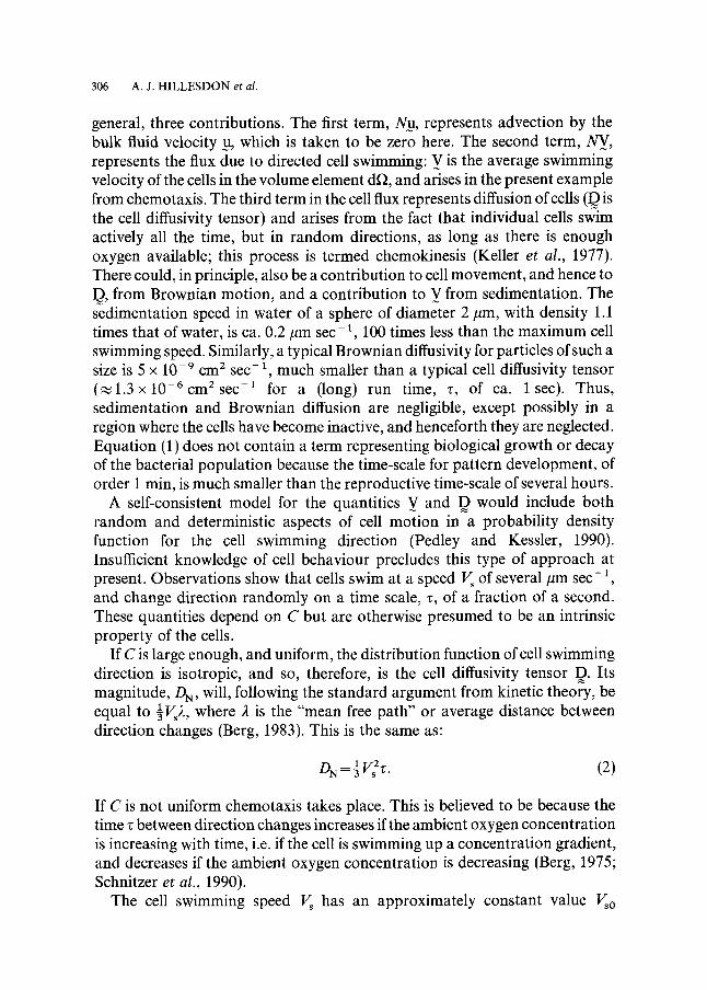
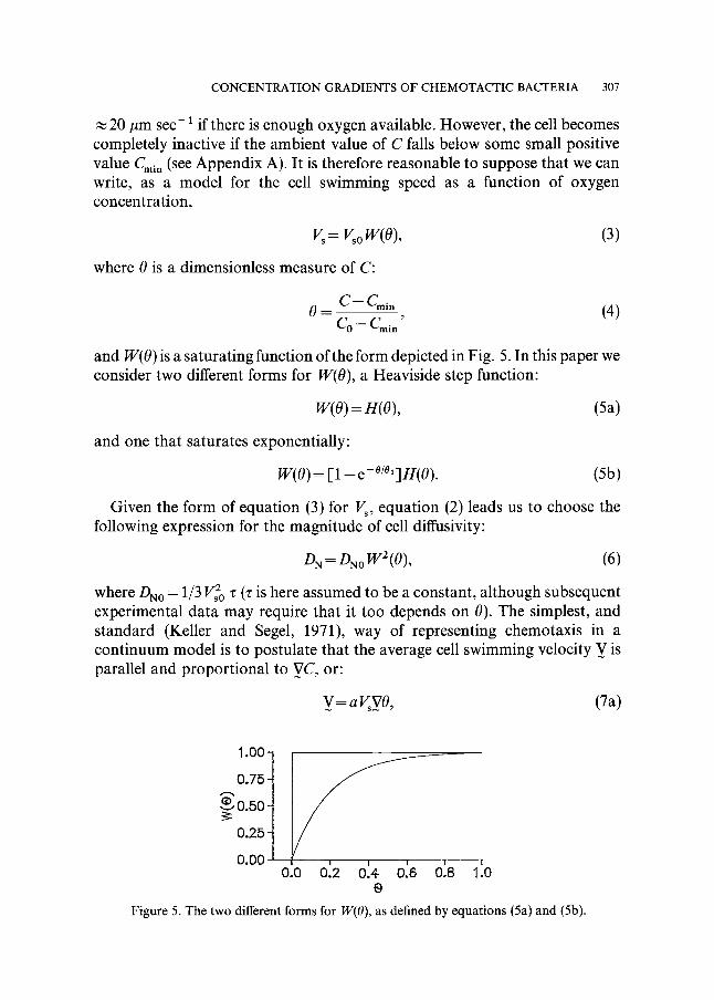
and W(O) is a saturating function of the form depicted in Fig. 5. In this paper we consider two different forms for W(O), a Heaviside step function:
W(O)=H(O), (5a)
and one that saturates exponentially:
W(O) = [1 - e-~176 (5b)
Given the form of equat ion (3) for V s, equat ion (2) leads us to choose the following expression for the magni tude of cell diffusivity:
DN=DNoW2(O), (6)
where DN0 = 1/3 V~o z ('c is here assumed to be a constant , a l though subsequent experimental data may require that it too depends on 0). The simplest, and s tandard (Keller and Segel, 1971), way of representing chemotaxis in a con t inuum model is to postulate that the average cell swimming velocity V is parallel and propor t ional to VC, or:
V = a V~V0, (7a)
1.00 -
, . 0 . 7 5 -
,0.50
0.25
0.00 I I I I I
0.0 0,2 0.4 0.6 0,8 1.0 0
Figure 5. The two different forms for W(O), as defined by equations (5a) and (5b).
308 A.J. HILLESDON e t al.
for some constant scale length, a. There may be a cut-off value of I VC[ below which chemotaxis does not occur. In order to investigate the consequence of that we also consider a case in which:
where:
y = a (Iv01- o)H(I V01- to), (7b)
yo=lv01 ,
and ae o is a small, positive, dimensionless number.
2.2. Oxygen concentration equation. The equation for oxygen concentra- tion, C, is also of the conservation type, but with an additional reaction term to represent the consumption of oxygen by the cells:
OC
~T - - - - V . ( C u - D c V C ) - K N . (8)
Here we assume that the flux of oxygen, by bulk advection and by diffusion, is not affected by the presence and motion of the cells: in principle the stirring motion generated by random cell movements would tend to increase the oxygen diffusivity, Dr, but the effect will be negligible unless/)NO is larger than D r . Since D r ~ 10- 5 cm 2 sec- 1, assuming it to be a constant is justified. The direct effect of the cells on C occurs through the consumption term KN. Here K is expected to be another saturating function of C, of the same form as that shown in Fig. 5, also switched offwhen the cells become inactive (for otherwise C could become negative). In fact, since we do not have any data on the functional dependence of K on C, we take it to be the same as for V~, i.e.:
K = K o W(O). (9)
2.3. Boundary conditions. The boundary conditions on the oxygen con- centration, C, are that it takes the given values C o (so 0 = 1) at any interface with the air, and that there is zero flux at all other boundaries. The boundary condition on the cell concentration, N, will be taken to be the obvious one of zero flux, balancing chemotaxis and cell diffusion, at all boundaries of the suspension. It should be recognized, however, that other boundary conditions are possible: for example, there is some evidence that a free surface can saturate with cells, and that as more cells arrive at the surface they stick to it, forming close-packed cell layers. The surface would act as a sink of cells, and this could be represented by a boundary condition of fixed cell concentration, say N = N s . This situation could affect the boundary condition on C, too. Such alternative boundary conditions will not be considered further here.
CONCENTRATION GRADIENTS OF CHEMOTACTIC BACTERIA 309
In this paper we seek to model the experiments shown in Fig. 3 and sketched in Fig. 4, with no bulk fluid motion. We therefore suppose that both 0 and N are functions of Z, the vertical coordinate, and T, the time, and that the boundary conditions are to be applied at the free surface, Z = 0, and the bottom of the suspension, Z = - h . The cells swim vertically upwards with speed V z given by the vertical component of equations (7a and b) with equation (3). The boundary conditions are, for all T~> 0:
80 0=1 at Z = 0 , ~ = 0 at Z = - h
0Z ON } (10)
VzN--DN ~-~ = 0 at Z = 0 , - h .
The initial, well-stirred condition, at T= 0, is that the suspension is uniform:
O(Z, 0)= 1, N(Z, 0 ) = N o. (11)
There is one further condition to be applied, that the total number of cells is conserved (since biological growth and decay are assumed negligible). Hence, for all T:
f~ N(Z, T)dZ=Noh. h
(12)
2.4. Non-dimensionalization. Equation (4) gives the dimensionless form, 0, of the oxygen concentration. We now introduce dimensionless forms of the other variables, as follows (note that the sign of Z has been reversed, for convenience):
n =N/No, z = -Z /h , t= (DNo/hZ)T. (13)
The governing equations [(1) and (8)] for the model now become:
8n_ 8 (W2(0)8/'/ (14)
o ost = (~176 - w(o).) , (15)
where W(O) is given by equation (5a or b) and the dimensionless constants are:
_ Do aVso _ / ( o N o h DN0, 7=DNo, DcAC, e=%h, (16)
310 A.J. HILLESDON et al.
with A C = C O - C m i n. Note that the square bracket in the second term on the r ight-hand side of equat ion (14) is equal to + 1 when 0 falls with distance below the free surface, as expected here (see Fig. 4).
The dimensionless boundary condit ions equat ion (10) are:
0(0, t )= 1, (17)
Oz (1, t )=O, (18)
0n + at (19)
with the initial conditions,
O(z, O) = n(z, O) = 1, (20)
and the integral constraint,
ff n d z = 1. (21)
2.5. Parameter values. Typical values of Vso, /)NO and D c were quoted above as Vso~20 #m sec -1, DNO~I.3 • 10 -4 m m 2 sec -1, Dc~10 -3 m m 2 sec -x. It is still neccessary to estimate the quantities K o, the oxygen consumption-ra te constant, a, the chemotaxis constant , and 5, the oxygen gradient cut-off. The former can be assessed from the time, T c, taken, in the experiment, for the cells below the critical depth h c to run out of oxygen. This appears to be of the order of 1-2 min, say T c ~ 100 sec. Now, scaling equat ion (8) suggests that:
AC --~KoNo, L
so, KoNo/AC~ 1/Tc~0.01 sec-1, and it follows that,
h 2 f12 _ ~ 10 h 2, (22)
OcT~
where h is measured in mm. Thus, fl is the appropriate dimensionless depth parameter; in the experiment shown in Fig. 3, fl is large ( ~ 25), while, even in the shallow layer experiment of Fig. 1, fl takes the value of ~ 8.
The chemotaxis constant, a, and hence the dimensionless constant 7, is more
CONCENTRATION GRADIENTS OF CHEMOTACTIC BACTERIA 311
difficult to estimate in the absence of detailed data on the statistics of cell trajectories. From equation (7a) the upswimming velocity is:
~0 V~aVso ;
a suitable time-scale for the concentration gradient must be AC divided by the critical depth ho, rather than the imposed suspension depth h, so V ~ a Vso/h ~ . Thus, the choice for the dimensionless a/hr is the ratio of average upswimming velocity to cell swimming speed. This can, in principle, take any value less than 1. From the definition of V we have:
a hr "
Y~hr /)No '
experiment (see Fig. 3) suggests that hc~5 mm, so ~ 8 0 0 (a/hc). If a/hr (= V/Vso ) is as small as 0.1, then ~ ~ 80, suggesting that ~ should be taken to be large when applying this model to the experiments on Bacillus subtilis. However, the above reasoning is based on a number of assumptions which need to be tested in more quantitative experiments.
The quoted values for De and/)No give 6 ~ 7. Finally, there are no data at all on the value of the "gradient cut-off" parameter e, if it exists. It is included in the calculations below to see what qualitative difference it makes to the results. A typical non-zero value will be taken to be 0.1.
3. Steady-State Solutions. In the steady state, ~n/Ot=~O/Ot=O; the cell- concentration equation [equation (14)] can then be integrated once, with the boundary condition of equation (19), to give zero cell flux for all z. The governing equations then become:
) W(O) dz = \ d z + e H dz ~ n, (23)
d20 dz 2 _ ~2 W(O)n, (24)
whenever W ( O ) ~ 0 . In section 2 two possible choices for W(O) were outlined. When W(O) is chosen to take the more complicated, yet more realistic, form of equation (5b) the task of solving equations (23) and (24) must be performed numerically. An analytical solution can be found if the step function form of equation (5a) is used, and therefore we concentrate on this form.
As observed experimentally, the evolution of the cell concentration profile
312 A.J. HILLESDON et al.
varies according to the depth of the chamber. It is correlated with the oxygen concentration. If the overall depth is sufficiently small (h < h~) 0 does not fall to zero anywhere; otherwise a zone where 0 = 0 and cells become inactive develops for z < - h~. These zones are described as the shallow- and deep-layer cases, respectively. The two cases are considered separately, with both zero and non-zero oxygen concentration cut-off gradients.
3.1. Shallow layer with e = 0. In all cases, consumption causes significant oxygen concentration gradients to form in the chamber. As a result of chemotaxis, cells gradually accumulate in the vicinity of the surface, forming a thin densely packed boundary layer. Immediately below this layer, experiment shows that there is a zone of significant cell depletion. From these observations it can be inferred that, in a shallow layer:
(1) 0 > 0 for 0~<z~<l; (2) OO/&<O for 0~<z<l ;
and that cell diffusion, cell chemotaxis and oxygen consumption are non-zero throughout. The (step-) function W(O) = - 1, and equations (23) and (24) can easily be manipulated to give the following equation for 0 only:
d30 d20 dO
dz 3 = 7 dz 2 dz" (25)
This is to be solved subject to the boundary conditions:
dO 0(0)= 1, d~ (1)=0, (26)
and, by equation (24) and the integral (21),
dO _f12. dz (0)= (27)
Wr i t i ng f ( z )=dO/ dz and integrating equation (25) twice gives:
f f m=~ - ( l - z ) , dl 7
~) f 2 + A 2
where A is an arbitrary constant. The possible solutions forfdepend on the sign of A. First, suppose A = - A 2 (A 1 >0). This gives:
f = A 1 [1-- exp( -- TA 1(1 --z))]/[1 + exp ( - 7A1(1 --z))],
but this is positive and cannot satisfy condition (27); the case A < 0 can
CONCENTRATION GRADIENTS OF CHEMOTACTIC BACTERIA 313
therefore be ruled out. The case A = 0 can also be discounted because the integral is singular at f = 0 (z= 1). Therefore, A = +A~ (A 1>0) is used. Integration gives:
f = dz -
Integrating once more, and applying the boundary condition 0(0) = 1, leads to the solution:
O(z)=l 2 COS 7-A 1 (29)
't cos0 ,) ) It also follows from equation (24) that:
The constant A 1 is determined by applying the remaining unused boundary condition (27), which leads to the following transcendental equation:
f12 tan( Ax)= 31, Clearly, for known values ofv and f12 there exists an infinite number of positive values for A 1 which satisfy this equation, and for each such value there corresponds a solution for O(z) and n(z). However, for all but the first, cos((v/2)Al(1-z)) changes sign in the range 0 < z < l , so the logarithm in equation (29) becomes singular. Therefore, the first zero, for which 0 ~<A 1 < re/V, must be chosen.
A further condition to be satisfied by the shallow layer solution is 0 1> 0, with equality only at the bottom, z = 1, if anywhere. Now, 0 is a monotonic decreasing function of z, from equation (28), so it is sufficient to require 0(1 ) >~ 0. From equation (29) this gives:
whence tan2((~/2)At) ~< 0.2, where 0 .2 = e ~ - 1. Then, from equation (31), we have:
(32)
314 A. J . H I L L E S D O N et al.
f12 ~<A1 o_ ~< 2 - tr t a n - l(tr). (33)
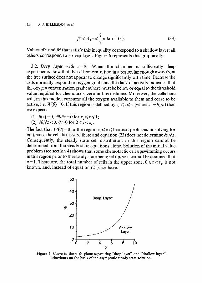
Values of 7 and f12 that satisfy this inequality correspond to a shallow layer; all others correspond to a deep layer. Figure 6 represents this graphically.
3 . 2 . Deep layer with e=O. When the chamber is sufficiently deep experiments show that the cell concentrat ion in a region far enough away from the free surface does not appear to change significantly with time. Because the cells normally respond to oxygen gradients, this lack of activity indicates that the oxygen concentrat ion gradient here must be below or equal to the threshold value required for chemotaxis, zero in this instance. Moreover , the cells here will, in this model, consume all the oxygen available to them and cease to be active, i.e. W(O) = 0. If this region is defined by z c ~< z ~< 1 (where zc = hr then we expect:
(1) O(z)=-O, O0/Oz=-O for zr (2) O0/Oz<O, 0 > 0 for O<<.z<z~.
The fact that W(O) = 0 in the region zr ~< z ~< 1 causes problems in solving for n(z), since the cell flux is zero there and equat ion (23) does not determine On~Oz. Consequently, the steady state cell distr ibution in this region cannot be determined from the steady state equations alone. Solution of the initial value problem (see section 4) shows that some chemotactic cell upswimming occurs in this region prior to the steady state being set up, so it cannot be assumed that n - 1 . Therefore, the total number of cells in the upper zone, O<<.z<zc, is not known, and, instead of equat ion (21), we have:
5 0 -
0 -
Deep 30-
20-
10 - ~ ShQIIow Layer
0 o 1'o
"7 Figure 6. Curve in the ]~__f12 plane separating "deep-layer" and "shallow-layer"
behaviours on the basis of the asymptotic steady state solution.
CONCENTRATION GRADIENTS OF CHEMOTACTIC BACTERIA 315
f~ ~ n dz = (34) ~c,
where ar is an unknown constant, defined by ~o n d z = 1 - a r and hence, presumably, lying in the range zr ~< ar < 1.
No problems are encountered in the region 0 <~ z ~< zr as both the oxygen concentration and its gradient are non-zero there. Proceeding as in section 3.1, it is found that:
and
dO_ z
/cos(Z _21nl. \2 ____ J.|, (36)
with the condition:
\2 (37)
tan A2z ~ - A2 , (38)
where A 2 is a positive constant. In the shallow layer case there was an unknown constant, A 1, determined by equation (31). In this case there are three unknown constants, A2, zr and ~r One additional equation arises from the requirement that O(zr so that:
O(z '=~ ln ( sec (2A2(zc - z ) ) ) , (36a)
and explicit expressions can be obtained for A 2 and zc in terms of ar fl and 7:
A 2 - ~ c f l 2 , ( 3 9 ) O"
_ 20" t a n - l(a). zo ~o3 ~ (4o)
316 A.J. HILLESDON et al.
As stated above, it is not possible in this analysis to calculate ~r its value must be estimated from the numerical results for the t ime-dependent case (see section 5). The steady state solutions can then be constructed analytically and compared with those calculated numerically, in order to establish the accuracy of the latter (again, see section 5).
Finally, it should be noted that the condi t ion z c ~< 1, needed for consistency of the deep layer solution, requires:
2o- 2 fiE ~>__ t a n - l(a) ~> _ a t a n - l(a),
precisely the converse of inequality (33), as expected.
3.3. Shallow layer with e r 0. In t roducing a non-zero cut-off gradient for the cell upswimming speed suggests that in the steady state there will be a region 0 ~< z < z* (say) where the cell swimming speed is non-zero and a region z* ~< z ~< 1 where it is zero. For reasons explained in the corresponding case with e = 0 (section 3.1), it is expected that 0 (z )>0 for all z e [0 , 1], so W(O)-1.
For the region z* ~< z ~< 1 the steady state equat ions (23) and (24) become:
dn - - = 0 , ( 4 1 ) dz
d 2 0 dz z =/~Zn. (42)
The solution to equat ion (41) is n = constant = na (say). Again, assuming that a small p ropor t ion of chemotactic cell upswimming occurs in this region prior to the steady state being set up, we may write:
fz l n dz = l - e*,
so that:
nl \a--z'J"
Consequently, from equat ion (42), is obtained:
(43)
(z2 ) O(z)=flZnl ~ - z +B 1, (44)
where the no-oxygen-flux condi t ion at z = 1 has been applied and B 1 is an
CONCENTRATION GRADIENTS OF CHEMOTACTIC BACTERIA 317
* is unknown constant. Additionally, the requirement that dO/dz = - e at z = z c satisfied only if:
8 nl -- f12(1-z*)" (45)
Equat ing (43) and (45) we find that:
o~* = 1 - e/fl 2, (46)
and is not arbitrary (unlike ac in section 3.2). In the region 0 ~< z < z* equations (23) and (24) can be combined to give:
d30 d20( dO ) dz3 = ? dTz 2
from which we find that:
COS -? A3(z* --z) (47)
The cell distribution obtained from equat ion (24) is:
n(z)=(-~)Z 2sec2(2Aa(z* - z ) ) , (48)
and upon application of the integral constraint it is found that:
tan(2 A3z*)--fl2~*A3 (49)
- * determines the constant B 1 Cont inui ty of the oxygen concentrat ion at z - z ~ and a further relation is obtained from continuity of the cell concentrat ion, which is required because the cell diffusivity, propor t ional to w a ( 0 ) = 1, is non-zero there. This gives:
nl= 2'
so, using equations (43) and (46), we obtain:
(50)
318 A.J. HILLESDON et al.
* in equation (49) we obtain a single implicit By substituting for A 3 and ~r equation that determines the position of the cut-off point z* for known values of e, 7 and f12. The steady state solutions for n(z) and O(z) are then known completely.
3.4. Deep layer with ~ # O. Here the features of the previous two sections are combined, and it is necessary to divide the chamber into three regions:
(1) Region 1: V#O, DN#O, O<<.z<z*, * ~ < Z < Z c (2) Region 2: V=0, DN#O, zr
(3) Region 3: V=0, DN=0, h<<.z<~l.
In terms of the dimensionless oxygen concentration, 0, we have:
(1) Region 1: 0<0~<1, t3Ofi3z<<. -e, (2) Region 2: 0~<0< 1, -e<<. ~O/~z<<. O, (3) Region 3: 0=0 , aO/Oz=O,
with continuity of both 0 and t30/~z at the interfaces z = zr and z = z*. The cell concentration n is continuous at z=z*, where t30/t~z=-e and On/tz=O. However, as in section 3.2, no condition on the continuity of n or its gradient can be imposed at z = z~ because D N = 0 for z >I zc.
Assuming that in the entire chamber the steady state and initial cell distributions are different we may write:
ndz+ ndz+ n dz=~* +ctxr 1. (51) * :c
Dividing the integral constraint in this way enables the analysis to be carried out independently in each of the regions defined above.
Region 1. In this region, as in section 3.3, equations (23) and (24) have the form:
d n ( d O ) d20 = + n , = 2n.
The cell and oxygen concentrations are again given by equation (47)-(49) for some positive c o n s t a n t A 3 .
Region 2. In equation (23) the term representing cell upswimming is zero in this region, so the steady state equations become:
dn O, d 2 0 d~= ~ = fl2n"
CONCENTRATION GRADIENTS OF CHEMOTACTIC BACTERIA 319
Proceeding as in section 3.3, we obtain:
n(z) = n 1 = (zc - z* )e/fl 2, (52)
O(z) = fl2n 1 (z 2/2 - zr + B2, (53)
where B 2 is a constant which can be determined using the continuity of 0 at z = z*, and:
~1c = (zr - z*)Ze/fl 2. (54)
Continuity of 0 and n at z = z * gives:
B 2 = l - e z ~ - In sec A3z* - - ~ z ~ t ~ - - z * ) ( z * - 2 z ~ ) , (55)
2 (56) A3z= 7
Region 3. Once again, as in the deep-layer case with e=O, the cell distribution cannot be determined in this region because both the cell flux terms in equation (23) and the oxygen consumption term in equation (24) are zero. It then follows that the constant Ctzc will be unknown and in order to find analytical steady state solutions its value must be estimated from the numerical solution of the initial value problem.
Applying the condition 0 = 0 at z = z~ we find from equation (53) that:
1 , 2 )zo.
Equating this expression with equation (55) gives an equation relating z c and zc*. Now ct c*-- 1-o~2c-(zr 2 and substituting this into equation (49) gives a second equation relating zr and z*. Solving these equations numerically for the two unknowns then gives the steady state solution.
That concludes the analysis of the steady state cell and oxygen distributions for the step function form of W(O). The results will be compared with those of the numerical solution of the initial value problem in section 5. Steady state results for the non-step function form for W(O) [equation (5b)], which require numerical solution anyway, are also given in section 5.
4. Solution of the Initial Value Problem. Here we return to the full time- dependent problem given by equations (14) and (15) with boundary, initial and integral conditions (17)-(21). This problem must be solved numerically in all
320 A.J. HILLESDON et al.
cases, even the simplest in which W(O) =- H(O) and e = 0. Only for short times is an analytical solution available, and we state its leading terms here, in the case e = 0, as a means of initializing and checking the numerical code.
4.1. Short time solutions. For short times 0 and n are expected to depart only a small amoun t from their initial values of 1. The first effect will be consumpt ion of oxygen by the cells, uniformly except near the surface where the diffusion of oxygen in from the a tmosphere generates a gradient. Then cells begin to swim up this gradient. Thus, if we write:
0 ~ 1 - 0 1 , n = l + n 1,
with 01 and n 1 small, the equations to be solved for 01 and n 1 are:
001 /'0201
subject to (57)
and
subject to
001_ 0 01(0, t ) = 0 , Oz as z ~ o o ,
On 1 02nl 0201 & - 0z 2 + y 0z ~
0nl 001 & + 7 &-z = 0 at z=O and as z ~ o o , (58)
f ~ n 1 d z = 0 . 0
The solutions of these equations are:
01 =fla &(err t /_2q2 erfc q + 2 t / e x p ( - q 2 ) / x / n ) + O ( t 2 ) , (59)
where t /= z / 2 ~ t . For 8 = 1,
n 1 =Tflzt((3t;2 + 1/2)erfc t / - 3 t / exp ( - t l z ) /x /n )+O( t2 ) , (60a)
and for 8 r 1,
27 6,8 2 t(q e x p ( - q 2 ) / g n - (,2 + 1/2)erfc t /+ x/8(x/n(1 - 8 ) - 1) nl = ( 8 - 1)
( t / e x p ( - 8q2)/x/(nS)- (tt 2 + 1/(28))ertc(x/Sq))). (60b)
CONCENTRATION GRADIENTS OF CHEMOTACTIC BACTERIA 321
These solutions are in agreement with the numerically computed results, shown in section 5, at short times.
4.2. The numerical solution for W(0)=H(0). Since the analytical steady state solution was obtained for the case in which W(O) is a step function, we concentrate on that case first in the numerical solution.
The numerical approach to this problem depends significantly upon whether we are dealing with a shallow or a deep layer, and the former case is much the simpler of the two and will be looked at first. The method will then be modified to deal with the additional difficulties (involving a moving boundary) that arise in the deep-layer case.
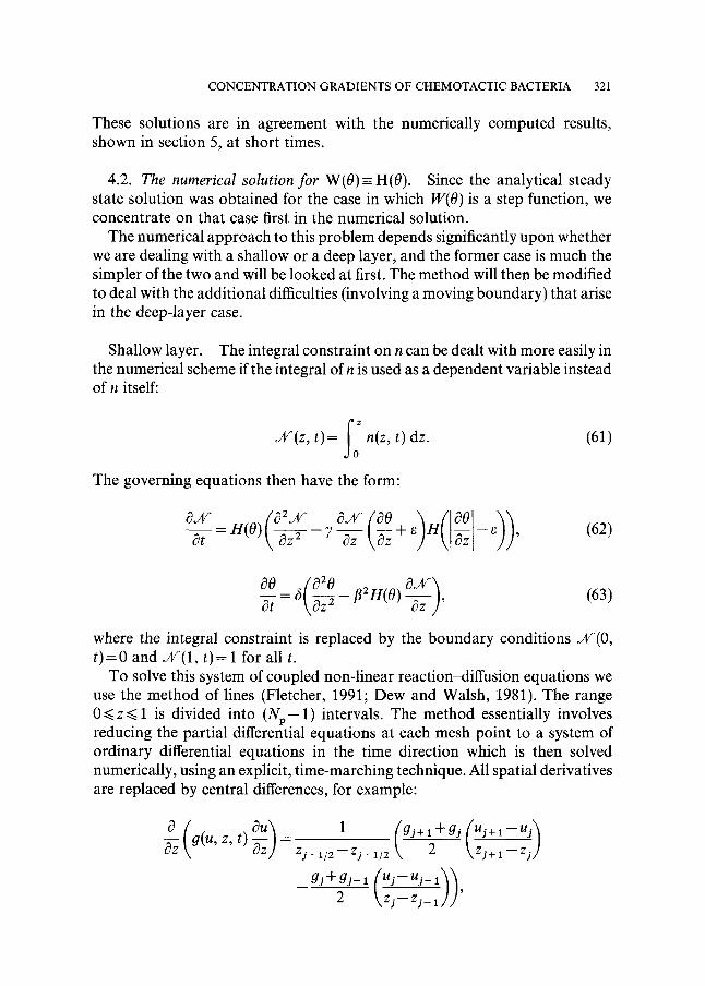
Shallow layer. The integral constraint on n can be dealt with more easily in the numerical scheme if the integral of n is used as a dependent variable instead of n itself:
Y(z , t)= ~o n(z, t) dz.
The governing equations then have the form:
(61)
/ \lOzl ' (62)
= - l 2H(O) / (63)
where the integral constraint is replaced by the boundary conditions Jff(0, t) = 0 and X(1 , t )= 1 for all t.
To solve this system of coupled non-linear reaction~liffusion equations we use the method of lines (Fletcher, 1991; Dew and Walsh, 1981). The range 0 ~<z ~< 1 is divided into (Np-1) intervals. The method essentially involves reducing the partial differential equations at each mesh point to a system of ordinary differential equations in the time direction which is then solved numerically, using an explicit, time-marching technique. All spatial derivatives are replaced by central differences, for example:
g(U, Z, t) ~Z Zj+I/2--Zj_I/2 2 \Zj+ x --Zj/
gj-Jc-gj-1 (Uj - -Uj - I~ , 2 \ z j - z j_~ / /
322 A.J. HILLESDON et al.
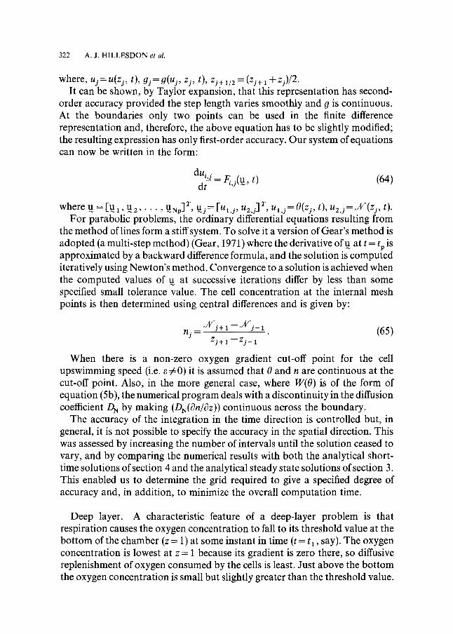
where, uj=u(zj, t), gj=g(uj, zj, t), Zj+ l/2= (Zj+ 1 + zj)/2. It can be shown, by Taylor expansion, that this representation has second-
order accuracy provided the step length varies smoothly and g is continuous. At the boundaries only two points can be used in the finite difference representation and, therefore, the above equation has to be slightly modified; the resulting expression has only first-order accuracy. Our system of equations can now be written in the form:
d u i . ~'J - F~,j(u, t) (64)
, . . . u r r , Y ( z j , t ) . where u = [u 1 u z, , -Np] , U j = [Ul, j, U2,j] Ul, j = O(Zj, t), Uz,j= For parabolic problems, the ordinary differential equations resulting from
the method of lines form a stiff system. To solve it a version of Gear's method is adopted (a multi-step method) (Gear, 1971 ) where the derivative of u at t = tp is approximated by a backward difference formula, and the solution is computed iteratively using Newton's method. Convergence to a solution is achieved when the computed values of u at successive iterations differ by less than some specified small tolerance value. The cell concentration at the internal mesh points is then determined using central differences and is given by:
J ~ j + 1 - - J ~ ' j - 1 nj = (65) Zj+ 1 - - Z j _ 1
When there is a non-zero oxygen gradient cut-off point for the cell upswimming speed (i.e. e ~ 0) it is assumed that 0 and n are continuous at the cut-off point. Also, in the more general case, where W(O) is of the form of equation (5b), the numerical program deals with a discontinuity in the diffusion coefficient Dr~ by making (DN(~n/~?z)) continuous across the boundary.
The accuracy of the integration in the time direction is controlled but, in general, it is not possible to specify the accuracy in the spatial direction. This was assessed by increasing the number of intervals until the solution ceased to vary, and by comparing the numerical results with both the analytical short- time solutions of section 4 and the analytical steady state solutions of section 3. This enabled us to determine the grid required to give a specified degree of accuracy and, in addition, to minimize the overall computation time.
Deep layer. A characteristic feature of a deep-layer problem is that respiration causes the oxygen concentration to fall to its threshold value at the bottom of the chamber (z= 1) at some instant in time (t = t 1 , say). The oxygen concentration is lowest at z = 1 because its gradient is zero there, so diffusive replenishment of oxygen consumed by the cells is least. Just above the bottom the oxygen concentration is small but slightly greater than the threshold value.
CONCENTRATION GRADIENTS OF CHEMOTACTIC BACTERIA 323
An instant later (t-=t2=t 1+At, say), consumption by the cells causes the oxygen concentration to fall to its threshold value at a slightly higher point, signifying an upward movement of the boundary at which 0 = 0. Below this boundary, at any instant, the cell diffusivity, cell upswimming speed and oxygen consumption rate are all zero and no immediate change in the cell (or oxygen) distribution will occur. As a result, from a numerical viewpoint, we need only find the n and 0 values above the moving boundary at any instant. Note that, prior to the propagation of a moving boundary, the numerical method employed in the shallow-layer case is sufficient to give solutions in the deep-layer case.
As the boundary position at any instant during its propagation is not known a priori we need to develop an algorithm that iteratively determines its position. Before explaining how the algorithm works we will show analytically that the oxygen conservation equation can be used to estimate not only when the boundary begins to propagate, but, for a limited period, its subsequent movement.
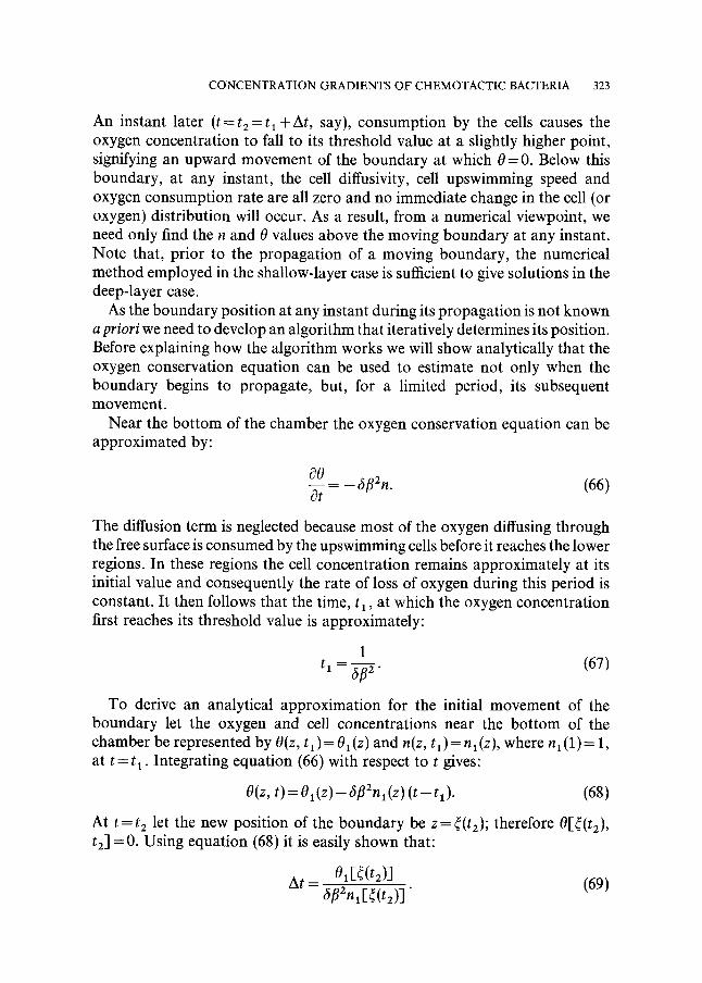
Near the bottom of the chamber the oxygen conservation equation can be approximated by:
00 Ot = -6f12n" (66)
The diffusion term is neglected because most of the oxygen diffusing through the free surface is consumed by the upswimming cells before it reaches the lower regions. In these regions the cell concentration remains approximately at its initial value and consequently the rate of loss of oxygen during this period is constant. It then follows that the time, t x , at which the oxygen concentration first reaches its threshold value is approximately:
1 tx = 6]~2" (67)
To derive an analytical approximation for the initial movement of the boundary let the oxygen and cell concentrations near the bottom of the chamber be represented by O(z, t l )= 01 (z) and n(z, t l )= n x (z), where n 1 (1)= 1, at t = t 1 . Integrating equation (66) with respect to t gives:
O(z, t) = 01 (z) - 6f12n, (z) ( t - t 1). (68)
At t = t 2 let the new position of the boundary be z= ~(t2); therefore 0[~(t2) , t2]----0. Using equation (68) it is easily shown that:
A t - - 01 [~( t2)] 6flZn,[~(t2)] . (69)
324 A.J. HILLESDON et al.
In the numerical scheme accurate tracking of the moving boundary requires that the change in boundary position over a small increment in time must be small. Therefore, equation (69) can be used to estimate the time-step needed to keep I~(ta)- ~(tl) I as small as required.
To illustrate how the algorithm works we will describe how the boundary position is found together with the solutions for Jff and 0 at t = ta, assuming that the solutions at t = t 1 are known.
Let ~(i)(t) denote the iterated value for the boundary position, where i = 1 corresponds to the initial guess. We now set up the boundary conditions at ~(i)(ta); these are:
(1) ~?O/Sz=O, (2) t2] = t l ] .
The first condition ensures continuity of oxygen concentration gradient across the boundary and the second condition assumes that, in the time interval At, cells become inactive in the region below the iterated boundary position so there is no cell flux across z=~(~ If z=~(~ does not correspond to a previously defined mesh point then at this point the current solutions ~ ( z , tl) and O(z, tl) will not be defined. To set up the initial solution for the next integration step these values are estimated by linear interpolation between the mesh points adjacent to ~(~ We then solve the problem using the method of lines (as outlined in the shallow-layer section) to obtain O(z, t:) and JV'(z, t2) in the region 0~<z~<~")(t2). For continuity of 0 across the boundary we require 0[~(~ t / I = 0 but, due to the limited machine precision, it is sufficient to specify that I 0[~(~ t:] I < Tol where Tol is a small user-defined value (typically Tol = O(10-6)). When this condition is satisfied we can proceed in a similar manner in order to find the subsequent boundary positions. Otherwise, a new guess for the boundary position must be made and the problem re-integrated from t = t~.
Note that in guessing the boundary position we are in effect trying to find the point where the increase in oxygen concentration, due to the downward flux of oxygen entering through the free surface, balances with the loss of oxygen due to consumption. Therefore, if O[~(i)(t2), tz] >Tol, the guessed boundary position is too close to the surface and must be increased, and if 0[~(~ t2] < - T o l , it is too far away and must be reduced.
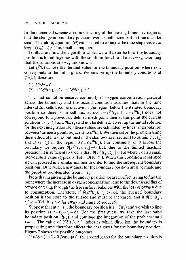
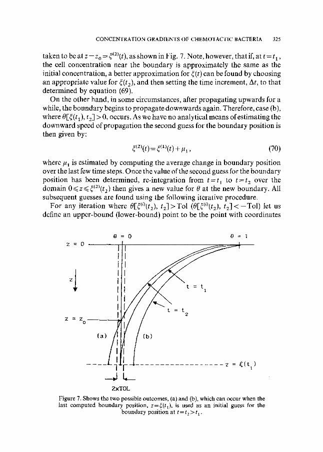
Suppose that at t = t~, the boundary position is z = ~(tt) and we wish to find its position at t=t2=t~+At. For the first guess, we take the last valid boundary position, ~(tl), and continue the integration of the problem until t = t 2. The value of 0[~(t~), t2] indicates which direction the boundary is propagating and therefore affects the next guess for the boundary position. Figure 7 shows the possible outcomes.
If 0[~(tt), t2] < 0 [case (a)], the second guess for the boundary position is
CONCENTRATION GRADIENTS OF CHEMOTACTIC BACTERIA 325
taken to be at z = z o = ~(2)(t), as shown in Fig. 7. Note, however, that if, at t = t l , the cell concentration near the boundary is approximately the same as the initial concentration, a better approximation for r can be found by choosing an appropriate value for ~(t2), and then setting the time increment, At, to that determined by equation (69).
On the other hand, in some circumstances, after propagating upwards for a while, the boundary begins to propagate downwards again. Therefore, case (b), where O[~(t 1), t2] > 0, occurs. As we have no analytical means of estimating the downward speed of propagat ion the second guess for the boundary position is then given by:
~(2)(t)=~(1)(t)+lq, (70)
where/ l I is estimated by computing the average change in boundary position over the last few time steps. Once the value of the second guess for the boundary position has been determined, re-integration from t = t 1 to t = t 2 over the domain 0 ~<z ~< ~(2)(t2) then gives a new value for 0 at the new boundary. All subsequent guesses are found using the following iterative procedure.
For any iteration where O[~(i)(t2), t2] > T o l (O[~(i)(t2), t 2 ] < - T o l ) let us define an upper-bound (lower-bound) point to be the point with coordinates
z = O
zi Z = Z
0
0 = 0
1
ca, 2xTOL
e = 1
/ t = t 2
z = ( ( t ) 1
Figure 7. Shows the two possible outcomes, (a) and (b), which can occur when the last computed boundary position, z=r is used as an initial guess for the
boundary position at t = t 2 > t 1 .
326 A. J . H I L L E S D O N e t al.
(O[~(i)(t2), t2] , ~(i)(t2) ). The next guess for the boundary position, r 1)(t2) ' is found by linear interpolation using the lowest upper-bound point and the highest lower-bound point. If no upper-bound (lower-bound) points have been found during the previous iterations, ~"+ 1~(t2) is found by linear interpolation using the lower-bound (upper-bound) points only. This process normally gives convergence to a solution in as few as five iterations.
5. Results and Discussion. In this section we look at the numerical results of the full time- and depth-dependent problem, as defined by equations (14) and (15), for particular shallow- and deep-layer cases with W(O) given by equations (5a) and (5b). In each case we are particularly interested in the following aspects:
(1) how do the cell and oxygen concentrations vary with time? (2) where applicable, what are the values of ~c, z c , . . , etc.? (3) how long does it take for the steady state to be set up? (4) how do the parameter values influence the results? (5) does imposing a non-zero cut-off gradient, e, for the cell upswimming
speed significantly alter the cell and oxygen distributions? (6) how does the choice of 141(0) affect the results?
Each case is solved using a non-uniform grid consisting of 501 points which, owing to the nature of the cell distribution, are clustered at the upper boundary in an attempt to reduce inaccuracies.
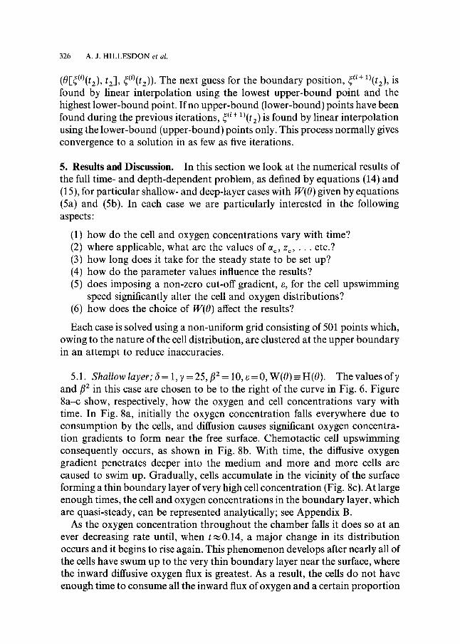
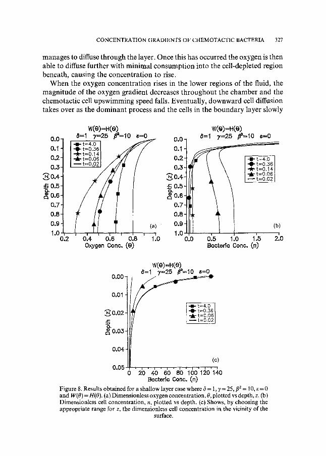
5.1. Shallow layer; ~ = 1, ~ = 25, f12 = 10, e = 0, W(0) ~ H(0). The values of~, and f12 in this case are chosen to be to the right of the curve in Fig. 6. Figure 8a-c show, respectively, how the oxygen and cell concentrations vary with time. In Fig. 8a, initially the oxygen concentration falls everywhere due to consumption by the cells, and diffusion causes significant oxygen concentra- tion gradients to form near the free surface. Chemotactic cell upswimming consequently occurs, as shown in Fig. 8b. With time, the diffusive oxygen gradient penetrates deeper into the medium and more and more cells are caused to swim up. Gradually, cells accumulate in the vicinity of the surface forming a thin boundary layer of very high cell concentration (Fig. 8c). At large enough times, the cell and oxygen concentrations in the boundary layer, which are quasi-steady, can be represented analytically; see Appendix B.
As the oxygen concentration throughout the chamber falls it does so at an ever decreasing rate until, when t ~0.14, a major change in its distribution occurs and it begins to rise again. This phenomenon develops after nearly all of the cells have swum up to the very thin boundary layer near the surface, where the inward diffusive oxygen flux is greatest. As a result, the cells do not have enough time to consume all the inward flux of oxygen and a certain proportion
C O N C E N T R A T I O N G R A D I E N T S O F C H E M O T A C T I C B A C T E R I A 327
manages to diffuse through the layer. Once this has occurred the oxygen is then able to diffuse further with minimal consumption into the cell-depleted region beneath, causing the concentration to rise.
When the oxygen concentration rises in the lower regions of the fluid, the magnitude of the oxygen gradient decreases throughout the chamber and the chemotactic cell upswimming speed falls. Eventually, downward cell diffusion takes over as the dominant process and the cells in the boundary layer slowly
0.0
0.1 0.2 0.3-
~,~ 0.4 ~0.5 | 0 . 6 r
0.7- 0.8 0 . 9
1.0 0.2
w(e)=H(e) ~=1 7=25 ,8==10 ~=0
I ' / s - 0 - t = 0 . 3 6 I �9 "~-- t = 0 . 1 4 1 -~. t=o.o6 I - - t=O.021
(a) I I
0.4 0.6 0.8 1.0 Oxygen Cone. (e)
~176 0.1 0.2 0.3
~ 0 . 4 s } & 0.6-
0.7- i 0.8 0.9-
1.0 0.0
w(e)=H(e) d=l ?,--25 #=--IO 8=0
, 4 - t = 4 . 0 \ I -e- t=0.36 I \ - ~ t=0.14 \ I ~ t=O.06 I
[ ~t=O.O2J
[
0[5 1.0 1.5 2~0 Bacteda Cone. (n)
0.00 -
0.01
~0.02
s 0.03
0.04-
0.05
w(e)=H(e) d=l ?,=25 ~=10 8=0
�9 i - t = O . 0 6 ~ t = O . 0 2
(c)
o 2'o 4:o 6'o 8'o 16o1~o14o Baeteda Cone. (n)
Figure 8. Results obtained for a shallow layer case where 6 = 1,7 = 25, f12 = 10, ~ = 0 and W(O) = H(O). (a) Dimensionless oxygen concentration, 0, plotted vs depth, z. (b) Dimensionless cell concentration, n, plotted vs depth. (c) Shows, by choosing the appropriate range for z, the dimensionless cell concentration in the vicinity of the
surface.
328 A.J. HILLESDON e t al.
disperse. As they do so, the oxygen flux that formerly entered the lower regions is again consumed and eventually a balance between diffusive oxygen replenishment and oxygen consumption develops. Simultaneously a balance between downward cell diffusion and upward cell chemotaxis arises and the steady state is reached. After t = 4 the cell and oxygen distributions change insignificantly with time and therefore provide a good approximation to the steady state.
The analytical steady state solutions, given by equations (29) and (30), where A a (=0.124666) is determined from equation (31), are graphically indis- tinguishable from the numerical solutions at t = 4.0.
5.2. Deep layer; ~ = 1, 7 = 10, f12 = 75, e = 0, W ( 0 ) - H(0). For convenience, the explanation of the results for this case is divided into three stages.
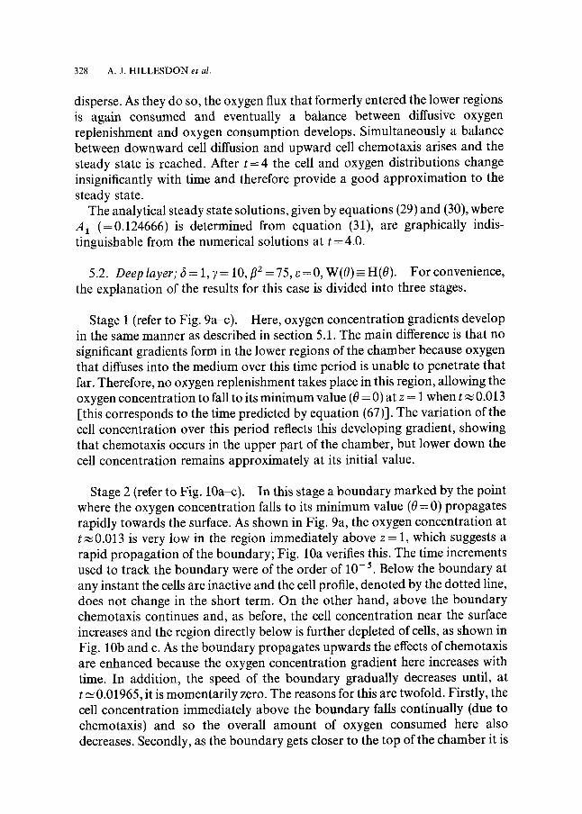
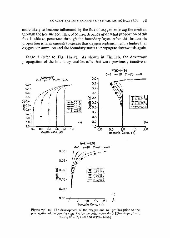
Stage I (refer to Fig. 9a-c). Here, oxygen concentration gradients develop in the same manner as described in section 5.1. The main difference is that no significant gradients form in the lower regions of the chamber because oxygen that diffuses into the medium over this time period is unable to penetrate that far. Therefore, no oxygen replenishment takes place in this region, allowing the oxygen concentration to fall to its minimum value (0 = 0) at z = i when t ~ 0.013 [this corresponds to the time predicted by equation (67)]. The variation of the cell concentration over this period reflects this developing gradient, showing that chemotaxis occurs in the upper part of the chamber, but lower down the cell concentration remains approximately at its initial value.
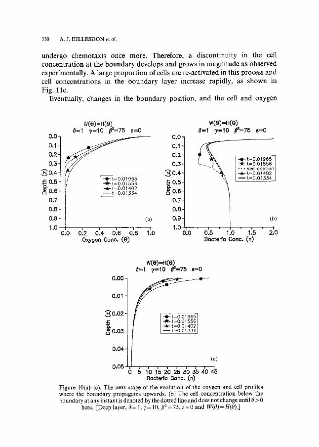
Stage 2 (refer to Fig. 10a-c). In this stage a boundary marked by the point where the oxygen concentration falls to its minimum value (0 = 0) propagates rapidly towards the surface. As shown in Fig. 9a, the oxygen concentration at t ~0.013 is very low in the region immediately above z = 1, which suggests a rapid propagation of the boundary; Fig. 10a verifies this. The time increments used to track the boundary were of the order of 10- 5. Below the boundary at any instant the cells are inactive and the cell profile, denoted by the dotted line, does not change in the short term. On the other hand, above the boundary chemotaxis continues and, as before, the cell concentration near the surface increases and the region directly below is further depleted of cells, as shown in Fig. 10b and c. As the boundary propagates upwards the effects of chemotaxis are enhanced because the oxygen concentration gradient here increases with time. In addition, the speed of the boundary gradually decreases until, at t-~ 0.01965, it is momentarily zero. The reasons for this are twofold. Firstly, the cell concentration immediately above the boundary falls continually (due to chemotaxis) and so the overall amount of oxygen consumed here also decreases. Secondly, as the boundary gets closer to the top of the chamber it is
CONCENTRATION GRADIENTS OF CHEMOTACTIC BACTERIA 329
more likely to become influenced by the flux of oxygen entering the medium through the free surface. This, of course, depends upon what proportion of this flux is able to penetrate through the boundary layer. After this instant the proport ion is large enough to ensure that oxygen replenishment is higher than oxygen consumption and the boundary starts to propagate downwards again.
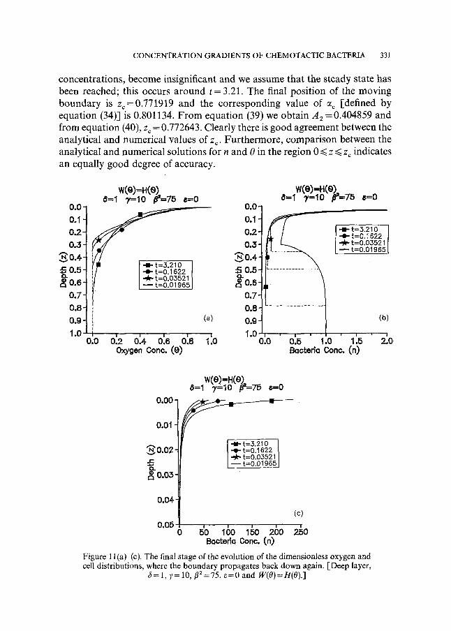
Stage 3 (refer to Fig. lla--c). As shown in Fig. l l b , the downward propagation of the boundary enables cells that were previously inactive to
w(e)=H(e)_ 6=1 "y:lO ~'=75 s=O
~176 y 0.1 0.2 0.5
v~-- 0-4 -e- t=0.013. -e- t=0.0106 ~ ~ -*- t:o.oos.
0.6 1 --e- t=o.o05~ - - t=0.0026 /
0"7 t 0.8 0.9 (a) 1.0 i
0.0 0.2 0.4 0.6 0.8 1.0 Oxygen Cone. (O)
0 . 0 -
0.1- 0.2- 0.5-
,~.,~ 0.4-- 0.5-
o _
o.e- 0.7-
0.8-
0.9-
1.0 0.0
w(e)=H(e) a=l ~=1o ~=75 ~=o
\ I I -e- t=o.o 106
"~1 --~ t=o.oo53. /] - - t=0.0026
(b) I I
0.5 1.o 1.5 ~o Bacteria (',one. (n)
w(e)=H(e) 8=1 -y=lO #==75 8=0
~176176 0.01 1
~_~0.02 1 Ill~~ ~ t=O.0106
0"05 6 <o 1'5 20 Baeteda Cone. (n)
Figure 9(a)-(c). The development of the oxygen and cell profiles prior to the propagation of the boundary marked by the point where 0 = 0. [Deep layer, ~5 = 1,
7 = 10, #2 = 75, ~ = 0 and W(O) = H(0).]
330 A.J . H I L L E S D O N et al.
undergo chemotaxis once more. Therefore, a discontinuity in the cell concentration at the boundary develops and grows in magnitude as observed experimentally. A large proport ion of cells are re-activated in this process and cell concentrations in the boundary layer increase rapidly, as shown in Fig. l l c .
Eventually, changes in the boundary position, and the cell and oxygen
0 ~
0.1
0.2
0 .3
.~,~ 0.4- 0.5-
Ct.
o.6-
0.7-
0.8-
0.9-
1.0 0.0
w(e)=H(e) 8=1 7=I0 ~=75 s=O
"-0- t=0.01965 - ~ t = O . O 1 5 5 6 - k - t = O . 0 1 4 0 2 - - t=0 .01334
' 0'.4 ' ' 0.2 0.6 0.8 Oxygen Cone. (O)
(a)
I
1.0
~176 t 0.1 0.2 0.3-
,.~0,4- s 0.5- o.. �9 0.6- ca
0.7- 0.8-
0.9-
1.0 0.0
w(e)=H(e) 8=1 7 = 1 o ~ = 7 5 s=o
:-e-t=o.o1965 -~ t=o .o1556 i . - -see caption --A-t=O,01402 - - t=0.01334
(b)
i i 1 0.5 1.0 1.5 2.0 Baeteda Cone. (n)
0.00
0.01
0.02 r
o_
0 .03
0.04-
w(e) =H(e) d=l 9,=10 ~=75 8=0
--~ t=O.O 1402 - - t=O.O 1554
(c) 0.05
o 1OlS O 53o3s Boeteda Conc. (n)
Figure 10(a)-(c). The next stage of the evolution of the oxygen and cell profiles where the boundary propagates upwards. (b) The cell concentration below the boundary at any instant is denoted by the dotted line and does not change until 0 > 0
here. [Deep layer, 6= 1, 7 = 10,/~2----75, •=0 and W(O)=H(O).]
CONCENTRATION GRADIENTS OF CHEMOTACTIC BACTERIA 331
concentrations, become insignificant and we assume that the steady state has been reached; this occurs around t = 3.21. The final position of the moving boundary is z~=0.771919 and the corresponding value of % [defined by equation (34)] is 0.801134. F rom equation (39) we obtain A 2 = 0.404859 and from equation (40), zc = 0.772643. Clearly there is good agreement between the analytical and numerical values of zr Furthermore, comparison between the analytical and numerical solutions for n and 0 in the region 0 ~< z ~< z~ indicates an equally good degree of accuracy.
0~
0.1- 0.2- 0.5-
~ 0 . 4 - ~0 .5 - = o . 6
0 .7 -
0 .8 -
0 .9 -
1.0 0.0
W(e)=H(O) ~=1 3,=10 ~ - 7 5 6--0
t=0.1622 t=0.03521 t=o.01965
i i i I
0.2 0.4 0.6 0.8 Oxygen Conc. (0)
(a)
I
1.0
w(e)=H(e) ~=1 7=10 #=--75 6=0
o oIs 0.1 0.2. -m- t=3.210 I
t=0.1622 0.5 -#P t=0.03521 I
t=O.O 1965 I ~ 0 . 4
s 0.511 ............... \ 1
o:;t . . . . . . . . . . . . . . . .
0.91 (b)
I"~ 0:5 1.o 1:5 s l~oteria Cone. (n)
0.00 -
0 .0 I
~o.o2
~0.03"
0.04"
0.05 0
w(e) =H(e). ~=1 7=10 F=75 6=0
-ii- t=3.210 -~ t=0.1622 --~ t=0.03521
t=o.01965
(c)
~o 16o I~O 260 2go Bootedo Conc. (n)
Figure 1 l(a)-(c). The final stage of the evolution of the dimensionless oxygen and cell distributions, where the boundary propagates back down again. [Deep layer,
3= 1, 7 = 10, fl2=75, s=0 and W(O)=H(O).]
332 A.J. HILLESDON et al.
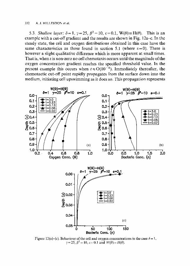
5.3. Shallow layer; 6=1 , 7=25, f12=10, e=0.1, W(0) -H(0) . This is an example with a cut-off gradient and the results are shown in Fig. 12a-c. In the steady state, the cell and oxygen distributions obtained in this case have the same characteristics as those found in section 5.1 (where e=0). There is however a slight qualitative difference which is more apparent at small times. That is, when e is non-zero no cell chemotaxis occurs until the magnitude of the oxygen concentration gradient reaches the specified threshold value. In the present example this occurs when t~O(10-4) . Immediately thereafter, the chemotactic cut-off point rapidly propagates from the surface down into the medium, initiating cell upswimming as it does so. This propagation represents
w(e)=H(e) ~-=1 ?,=25 0==10 e--0.1
0 .0 - 0 .1 - -=-t=3o -0- t=0.23 0.2- -~ t=0.13
- i - t=O.06 0.3- - - = -
v~.,0.4-
~ 0 . 5 -
0 . 8 o 1/ 0.8
1.0 , I !
0.2 0.4 0.6 0.8 1.0 Oxygen Cone. (e)
0 . 0 "
0.1- 0.2- 0.3-
~,,~ 0.4- ~ 0 . 5 -
o . e -
0.7-
0 .8 -
0 .g -
1.0 0.0
w(e)=H(e)_ ~=I 7=25 0==10 e---O,l
\ =ll- t=3.o t=0.23
-=Jr- t=0.13 -k" t=O.06 - - t=O.02
(b)
0.5 1.0 1.5 0 ~cter~a Cone. (n)
w(e) =H(e) ~=1 7=2-5 0==10 6=0.1
0.01
1 0.03
0.04]
0.05 o e o 16o
Bacteda Cone,. (n)
(c)
Figure 12(a)-(c). Behaviour of the cell and oxygen concentrations in the case 6 = 1, 7=25, f12=10, e=0.1 and W(O)=H(O).
CONCENTRATION GRADIENTS OF CHEMOTACTIC BACTERIA 333
a different sort of moving boundary, but no special numerical techniques are required to track it.
Below the boundary changes in the cell distribution are entirely attributed to cell diffusion. Comparing the cell profiles in Figs 8b and 12b at t = 0.06 reveals, as expected, that when e ~ 0 less cell upswimming in the lower regions of the chamber (and indeed everywhere) has occurred. Whilst the oxygen concentra- tion is decreasing its gradient in the upper regions increases thus ensuring the downward propagation of the chemotactic cut-off point. When t,,~0.13 this cut-off point is situated at z=0.938751 and a significant amount of cell upswimming even near the bot tom of the chamber has occurred. After this instant the oxygen concentration begins to increase (for reasons explained previously) and as a result the chemotactic cut-off point propagates upwards
* 0.726549 and the until the steady state is reached. Its final position is z c = * is 0.989999. As indicated by the results, the corresponding value of ac
behaviour of the cell and oxygen profiles during the approach to the steady state is similar in both the e = 0 and e r 0 cases.
To provide a check upon the numerical steady state solutions the steady state position of the chemotatic cut-off point, z*, can be calculated numerically by solving equations (49) and (50) where, from equation (46), a* = 0.99. We find,
* = 0.726575 which is in agreement using the Newton-Raphson method, that z~ with the estimated value above. The analytical steady state cell and oxygen distributions, given by equations (44), (45), (47) and (48) where A 3 = 0.171051, are graphically indistinguishable from the numerical steady state results and are therefore not included in the figures.
5.4. Deep layer; 6= 1, 7= 10, f12 =75, e=0.1, W(0)--H(0). Stage 1. The development of the cell and oxygen distributions in this stage
is practically identical to the corresponding case with e = 0. The only notable difference is that slightly less cell upswimming occurs in the e 4= 0 case.
Stage 2. Here the effect of less chemotactic cell upswimming is that the overall amount of oxygen consumption is high everywhere except in the boundary layer because a higher proportion of cells, compared to the e = 0 case, are situated in these regions. As a result the boundary reaches its uppermost point slightly more quickly than for e = 0 (t = 0.01952 instead of t = 0.01965).
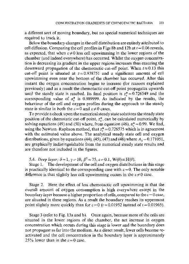
Stage 3 (refer to Fig. 13a and b). Once again, because more of the cells are situated in the lower regions of the chamber, the net increase in oxygen concentration which occurs during this stage is lower and the boundary does not propagate as far into the medium. As a direct result, fewer cells become re- activated and the cell concentration in the boundary layer is approximately 25% lower than in the e = 0 case.
334 A.J. HILLESDON et al.
The steady state position of the chemotactic cut-off point, computed numerically, is z* = 0.618980 and the corresponding value of ct* is 0.710850. In addition, it is found that the value of z c (as defined in section 3.4) is 0.703350 and the value of cqc is 0.001420.
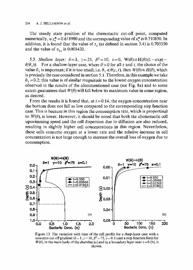
5.5. Shallow layer; 6 = 1 , 7=25 , # 2 = 1 0 , e = 0 , W(O)=H(O) (1 -exp ( - 0/01) ). For a shallow-layer case, where 0 > 0 for all z and t, the choice of the value 01 is important; if it is too small, i.e. 01 < O(z, t), then 141(0)~ H(O), which is precisely the case considered in section 5.1. Therefore, in this example we take 01 = 0.2; this value is of similar magnitude to the lowest oxygen concentration observed in the results of the aforementioned case (see Fig. 8a) and to some extent guarantees that W(O) will fall below its maximum value in some region, as desired.
F rom the results it is found that, at t = 0.14, the oxygen concentration near the bo t tom does not fall as low compared to the corresponding step function case. This is because in this region the consumption rate, which is proportinal to W(O), is lower. However, it should be noted that both the chemotactic cell upswimming speed and the cell dispersion due to diffusion are also reduced, resulting in slightly higher cell concentrations in this region. Nevertheless, these cells consume oxygen at a lower rate and the relative increase in cell concentration is not large enough to increase the overall loss of oxygen due to consumption.
o.o 1
0"I I 0 . 2
0 . 3
,~,0.+
~ 0o5 -
0 . 6 - t 0.7- -- 0 . 8 -
0 . 9 -
1 ,0 0 . 0
w(e) 8=1 ),=1o #~-75 a=o.1 0.001
14-t=9.550 , 0"01 1 -o- t=0.05966 - - t=0.01952 '~' 0"02 i
(a) 0"0+ 1 0.05
9'-o o
W(e) =H(e) 8=1 ?,=10 #=--75 s=0.1
I/ I - i- t=0.05966 / I -~" t=0.02305 ' I - - t=0.01952
! !
1.o 1.5 ~ e d a ~ n o . (n) ~cte~a ~no . (n)
(b) , s
16o 1go 260
Figure 13. The variation with time of the cell profile for a deep-layer case with a non-zero cut-off gradient (6 = 1, ? = 10, #z = 75, e = 0.1) and a step function form for W(O), in the main body of the chamber (a) and in a boundary layer near z = 0 (b), is
shown.
CONCENTRATION GRADIENTS OF CHEMOTACTIC BACTERIA 335
Near the surface of the chamber O(z, t)>> 01 , and consequently the cell and oxygen concentrations here are very similar to those observed in Fig. 8c. After t=0.14 the qualitative behaviour of the cell and oxygen distributions is the same as in the corresponding step function case and need not be explained. The quantitative differences occur purely because, during the time evolution, W(O) falls initially but then, as the steady state is approached, rises to a value close to its maximum.
5.6. Deep layer; 6=1, 7=10, fl2=75, s=0 , W(O)==-H(O)(1-exp(- 0/01). For this case the results are directly compared to those of section 5.2 in order to establish any difference that arises due to the imposition of a non-step function form for W(O).
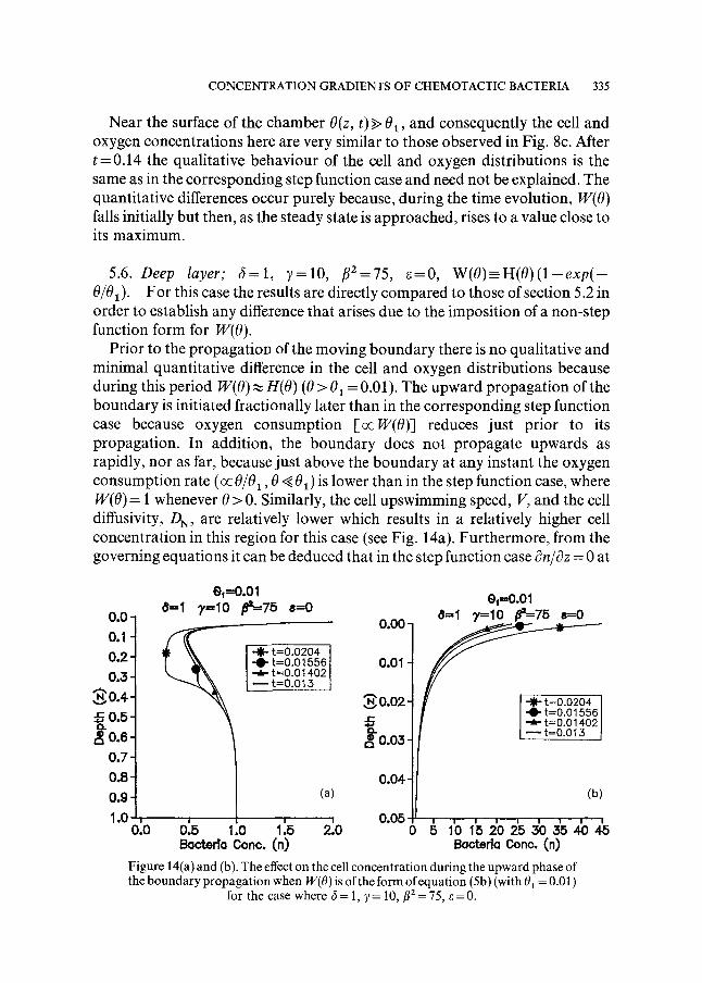
Prior to the propagation of the moving boundary there is no qualitative and minimal quantitative difference in the cell and oxygen distributions because during this period W(O)~ H(O) (0 > 01 = 0.01). The upward propagation of the boundary is initiated fractionally later than in the corresponding step function case because oxygen consumption [ocW(0)] reduces just prior to its propagation. In addition, the boundary does not propagate upwards as rapidly, nor as far, because just above the boundary at any instant the oxygen consumption rate (oc 0/01,0 ~ 01) is lower than in the step function case, where W(O) = 1 whenever 0 > 0. Similarly, the cell upswimming speed, V, and the cell diffusivity, DN, are relatively lower which results in a relatively higher cell concentration in this region for this case (see Fig. 14a). Furthermore, from the governing equations it can be deduced that in the step function case c~n/c3z = 0 at
0o0 ~
0.1-
0.2- 0.3-
v~0.4-
~ 0.5
0.6 0.7-
0.8 0.9 1.0
0.0
0,--0.01 8=I ?,=I0 #~--75 8=0
-!~ t=0.0204 -0- t=0.01556
t=O.O 1402 - - t=0.013
(a)
0.5 1.o 1:5 s l ~ c t e d a Cone. (n)
0 . 0 0 -
O.Ol -
, .~ 0 . 0 2 -
a~'O.03 -
0.04-
0,05 0 g
0,=0.01 8=1 ?,=10 ~=75 8=0
-0- t=O.01556 [ r ~ t=0.01402 I
-- t=o.o13 j
(b)
i - - i 1'0 3'0 4o Bacteda Cone. (n)
Figure 14(a) and (b). The effect on the cell concentration during the upward phase of the boundary propagation when W(O) is of the form of equation (5b) (with 01 = 0.01)
for the case where 6=1 , y=10,/~2 = 75, ~=0.
336 A.J. HILLESDON et al.
the boundary (where 0 = 0, ~O/~?z = 0) at any instant, whereas, in the current case, dn/Oz is undetermined at the boundary. Comparison of Figs 14a and 10b verifies this point.
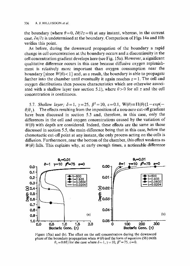
As before, during the downward propagation of the boundary a rapid change in cell concentration at the boundary occurs and a discontinuity in the cell concentration gradient develops here (see Fig. 15a). However, a significant qualitative difference occurs in this case because diffusive oxygen replenish- ment is relatively more important than oxygen consumption near the boundary [since W(O) < 1] and, as a result, the boundary is able to propagate further into the chamber until eventually it again reaches z = 1. The cell and oxygen distributions then possess characteristics which are otherwise associ- ated with a shallow layer (see section 5.1), where 0 > 0 for all z and the cell concentration is continuous.
5.7. Shallow layer; 6=1 , ;~=25, f l 2 = 1 0 , e=0.1, W(O)=-H(O)(1-exp( - 0/01)" The effects resulting from the imposition of a non-zero cut-off gradient have been discussed in section 5.3 and, therefore, in this case, only the differences in the cell and oxygen concentrations caused by the variation of W(O) with depth are considered. Indeed, these effects are the same as those discussed in section 5.5, the main difference being that in this case, below the chemotactic cut-off point at any instant, the only process acting on the cells is diffusion. Furthermore, near the bot tom of the chamber, this effect weakens as W(O) falls. This explains why, at early enough times, a noticeable difference
0.01 0.1 "1 0.21 0.3"]
I ~ 0.5- 0.6- 0.7- 0.8- 0.g- 1.0
0.0
1~I---0.01 ~=1 ?,=10 ~t=-75 6=0
0.5 1.o 1:. BQcterlo Conc. (n)
-$'t=600 "0"t=0.935 -'k-t=O.0600 ~t=0.0204
0.001
0.01 ] 30.021
0.~-
0 . 0 4 -
(a)
~0 0.05 0
e,--O.Ol
- I " t=600 -e.t=o.93s -~" t--O.0600
t=0.0204
16o 260 Bocteda Cone. (n)
(b)
Figure 15(a) and (b). The effect on the cell concentration during the downward phase of the boundary propagation when W(O) isof the form of equation (5b) (with
01 =0.01) for the case where 6= 1, 7= 10, f12 =75, e=0.
CONCENTRATION GRADIENTS OF CHEMOTACTIC BACTERIA 337
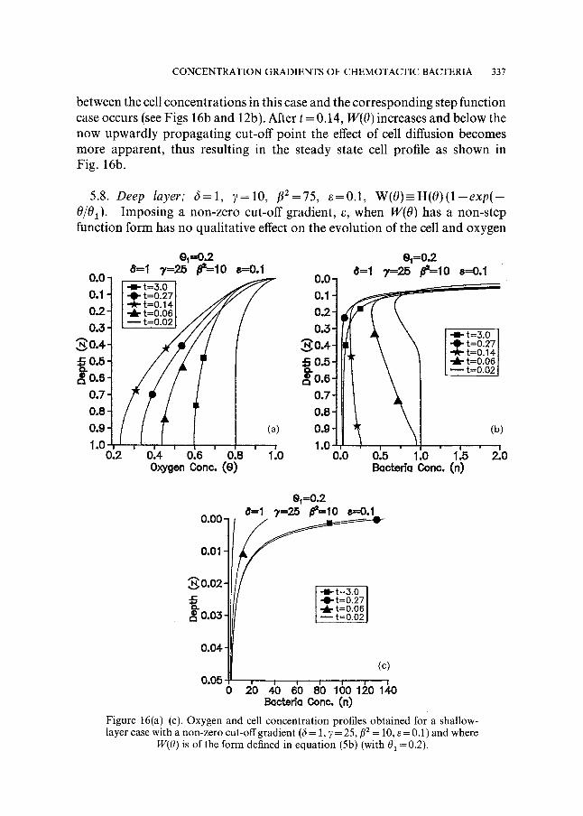
between the cell concentrat ions in this case and the corresponding step function case occurs (see Figs 16b and 12b). After t = 0.14, W(O) increases and below the now upwardly propagat ing cut-off point the effect of cell diffusion becomes more apparent , thus resulting in the steady state cell profile as shown in Fig. 16b.
5.8. Deep layer; 6 = 1 , 7=10 , f l2=75, e=O.1, W(O)-H(O)(1--exp(- 0/01). Imposing a non-zero cut-off gradient, e, when W(O) has a non-step function form has no qualitative effect on the evolution of the cell and oxygen
el--o.2 ~=1 7=25 p~--lO a---o.1
0.1 -0- t=0.27 t--0.14
0.2 ~ t=O.06 /~. 03 I m t=O.O217
Y / _ / a0.q ~ 0.5- / !
0.6- 0 . 7 -
0 . 8 -
0.9 - (a)
1.0" 0.2 0.4 0.6 0.8 1 '.0
Oxygen Conc. (e)
e1=0.2 t = l 7=25 #==10 8=0.1
o
0.1 0.2
03 4 - t=3.0 -0- t=0.27 -.A.- t=o.14
0.5 -I II T \ ~ t=O.06
o.,tll / \ o., ~ l 1.0 , , ,
0.0 0.5 .0 1.5 0 I~c~de Conc. (n)
el =0.2 ~=1 7=25 p==lO ~==0.1
0.01
o.o2 ll/ + t = 3 . 0 t
~0 ^~/il l I -A- t=o o6 I "u~ I I - - t=~176
0 . 0 5 ~ 0 20 40 60 80 100 120 140
l~ctedo Cone. (n)
Figure 16(a)-(c). Oxygen and cell concentration profiles obtained for a shallow- layer case with a non-zero cut-off gradient (6 = 1, 7 = 25,/~2 = 10, e = 0.1) and where
W(O) is of the form defined in equation (5b) (with 01 =0.2).
338 A.J. HILLESDON et al.
distributions although, as expected, a slight quantitative difference occurs. This difference can be explained using the same arguments as in section 5.4 and is therefore not discussed here.
5.9. Further discussion. From the results it is clear that there is an insignificant qualitative effect on the development of the cell and oxygen concentrations when a non-zero cut-off gradient for the cell upswimming speed is incorporated. We now discuss how variations in the parameters 8, 7 and/32 in the cases considered in sections 5.1 and 5.2 affect the time evolution of the cell and oxygen concentrations.
Increase 7 (8 and/32 fixed). An increase in the value of 7 (~ directly enhances the overall amount of cell upswimming causing higher cell concentrations in the surface boundary layer. In addition, the cells vacate the lower regions of the chamber more rapidly and therefore less overall oxygen consumption occurs in these regions. In a deep layer, this results in less overall upward movement of the boundary and, in the steady state, it is situated closer to the bot tom of the chamber. However, the overall qualitative behaviour of the cell and oxygen concentrations is not altered.
Decrease/32 (7 and c5 fixed). Any decrease in fi2 signifies a decrease in the depth, h, of the chamber which causes a relative increase in diffusive oxygen replenishment throughout the chamber. Not only is the net loss of oxygen in the chamber reduced, but so too is the oxygen concentration gradient at any instant. In a deep layer this means that the vertical distance travelled by the moving boundary is reduced. More generally, cell upswimming decreases, causing fewer cells to congregate in the boundary layer. As a result, the amount of oxygen able to penetrate through the boundary layer decreases. In a shallow layer this causes the oscillation in the oxygen concentration to become less pronounced, and in a deep layer, the steady state position of the moving boundary becomes closer to the bot tom of the chamber. Moreover, in the latter case, if/32 is reduced sufficiently, then a transition from a deep layer to a shallow layer takes place, in agreement with Fig. 6.
Increase 8 (7 and/32 fixed). In a shallow layer, when 8 is increased by a sufficient amount a significant change in the qualitative behaviour of the cell and oxygen distributions occurs. From the results, initially the net loss of oxygen (particularly near z = 1) is so great that the oxygen concentration falls rapidly to its threshold value and a moving boundary propagates upwards just as in a deep-layer case. Eventually the boundary stops (momentarily) and then reverses its direction of propagation. As it travels back towards z = l a discontinuity in the cell concentration develops and the re-activation of the
CONCENTRATION GRADIENTS OF CHEMOTACTIC BACTERIA 339
previously inactive cells causes a much higher proportion of cell upswimming. However, unlike a deep-layer case, the boundary propagates back to z = 1 and the discontinuity in the cell concentration disappears. After this the oxygen concentration increases above its threshold value and the cell and oxygen profiles are more reminiscent of a typical shallow-layer case. Notably, the steady state is reached much more rapidly (measured in the dimensionless time- scale) and, in addition, the cell and oxygen distributions are invariant to any change in the value of ~ (provided y and/32 remain fixed). This result is not surprising, since the analytical steady state solutions given by equations (29)-(31) are independent of 3.
To explain the qualitative differences described above it is neessary to consider how an increase in 6 relates to the original dimensional parameters. Since 6 = Dc/DNo, an increase in 6 can be viewed as either a decrease in/)No (with Dc fixed) or an increase in D~ (with/)No fixed). If the former is true, the value of ~ ( = a Vso/DNo ) is unchanged only if a Vso (ac VN) decreases by the same proportion. Consequently, cell upswimming is smaller and, because the cells spend relatively more time in the lower regions of the chamber, increased oxygen consumption occurs here. This is the reason why the oxygen concentration falls to its minimum value. The explanation of the subsequent behaviour of the cell and oxygen distributions has already been considered (see section 5.1). The dimensionless time-scale t is proportional to/)No and, hence, the steady state is reached more rapidly.
If De is increased (Duo fixed) then/32 remains constant only if (KoNo h 2/AC) increases by an equal proportion. If it is assumed that this increase is attributed to an increase in the depth, h, then once again a higher amount of oxygen consumption in the lower regions of the chamber (where diffusive oxygen replenishment is least) will occur resulting in the behaviour observed in the results. In addition, toc 1/h 2, and so the time it takes for the steady state to be reached reduces, as observed.
These ideas can also be applied to a deep-layer case. The effective decrease in V, caused if the case where Duo is decreased (with De fixed) is considered, results in reduced cell upswimming throughout the chamber during the upward propagation of the boundary. As a direct result the distance travelled by the moving boundary increases (due to the relative overall increase in oxygen consumption) during this phase of its motion. As before, after this phase, the boundary propagates downwards until it reaches its steady state position, z*, which is situated nearer to the surface than before. Note too that the corresponding value of e* also decreases. The downward distance travelled by the boundary, which depends on the overall amount of oxygen consumption, falls because relatively more cells are situated in the lower regions of the chamber thereby creating a greater "barrier" to diffusive oxygen replenish- ment. In addition, during this phase the oxygen concentration gradient near
340 A. J . H I L L E S D O N et al.
the surface is relatively higher and any cells that become re-activated swim upwards at greater speed. The result is that the cell concentration near the surface increases and the region from which the cells have swum from becomes even more depleted. Interpreting this result experimentally, one would observe a more well-defined discontinuity in the cell concentration and a thinner, more densely packed, cell boundary layer at the surface.
By investigating many other deep-layer examples it has been found that, if 7 and f12 a r e chosen so that the corresponding point in the 7-fl 2 parameter space of Fig. 6 is close enough to the c u r v e f12 : (2a/7) t an - 1 a, then the effect upon the steady state solutions of varying the value of 6 becomes less pronounced. The converse of this result, where the chamber depth effectively increases, is also true. Furthermore, for any point on the curve the steady state results are, as expected from the shallow-layer results, totally independent of 6.
6. Conclusion: Comparison With Experiment. The numerical results of the mathematical model for the pre-instability stage of the pattern formation process show certain qualitative features in common with experimental observation. Firtly, for both shallow and deep chambers, a densely packed cell layer develops in the vicinity of the surface (when 7 is sufficiently large). Secondly, for deep layers a discontinuity in the cell concentration arises because an insignificant amount of cell upswimming occurs before a region close to the bot tom of the chamber becomes starved of oxygen. This is in marked contrast to the region above, where significant gradients of oxygen, the cause of chemotaxis, occur. Furthermore, from experimental observation it is known that the discontinuity propagates and becomes more well defined with time. This too agrees with the results of the model.
For particular choices of 6, 7 and f12 a propagating discontinuity in the cell concentration, which at first travels towards the surface but later reverses direction and travels down to the bot tom of the chamber, has been predicted by the mathematical model. This behaviour has not yet been reported experimen- tally and a further investigation for chambers of various depths needs to be carried out. Of course, the behaviour may just be a product of the assumptions applied in our model. Therefore, other models with, for instance, a different boundary condition on the cell concentration at the upper surface (see section 2.3), or different assumptions for the cell swimming speed, cell diffusivity, etc., may need to be considered in order to establish whether or not this behaviour still occurs. Indeed, better quantitative agreement between the model and experimental results may be achieved when more experimental data concern- ing the functional dependence of DN, V N and K, on the oxygen concentration, becomes available.
The authors would like to thank the Science and Engineering Research Council
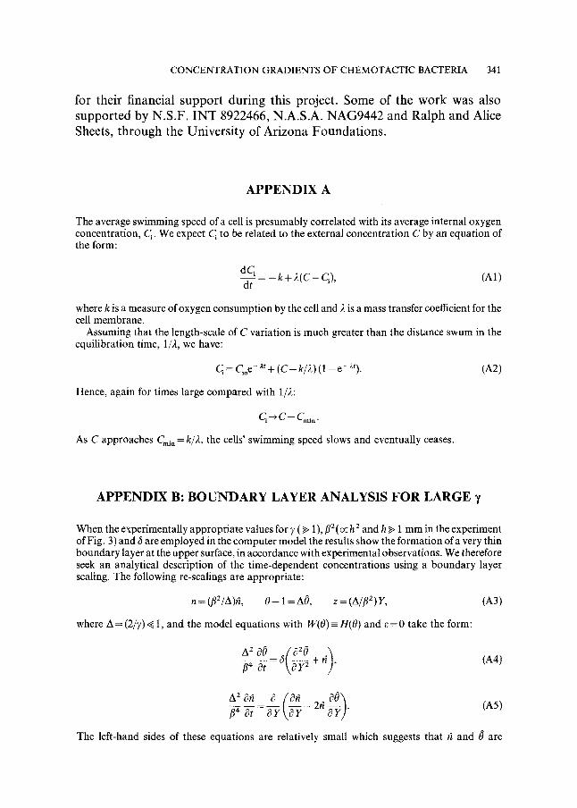
CONCENTRATION GRADIENTS OF CHEMOTACTIC BACTERIA 341
fo r the i r f inanc ia l s u p p o r t d u r i n g this p ro j ec t . S o m e o f the w o r k w a s a l so s u p p o r t e d b y N . S . F . I N T 8922466, N . A . S . A . N A G 9 4 4 2 a n d R a l p h a n d Alice
Shee ts , t h r o u g h the U n i v e r s i t y o f A r i z o n a F o u n d a t i o n s .
A P P E N D I X A
The average swimming speed of a celt is presumably correlated with its average internal oxygen concentration, C i. We expect q to be related to the external concentration C by an equation of the form:
dCi_ dt
- - - - k + 2 ( C - C O, (A1)
where k is a measure of oxygen consumption by the cell and 2 is a mass transfer coefficient for the cell membrane.
Assuming that the length-scale of C variation is much greater than the distance swum in the equilibration time, 1/2, we have:
G = C~oe- ~* + (c-k/,t)(1 - e - z*).
Hence, again for times large compared with 1/2:
(n2)
G--' C-- Cmin.
As C approaches Cml . --k/2, the cells' swimming speed slows and eventually ceases.
A P P E N D I X B: B O U N D A R Y L A Y E R A N A L Y S I S F O R L A R G E ~/
When the experimentally appropriate values for y ( >> 1), f12 (oc h 2 and h ~ 1 mm in the experiment of Fig. 3) and 6 are employed in the computer model the results show the formation of a very thin boundary layer at the upper surface, in accordance with experimental observations. We therefore seek an analytical description of the time-dependent concentrations using a boundary layer scaling. The following re-scalings are appropriate:
n=(fl2/A)fi, 0 - 1 = A 0 , z=(A/fl2)Y, (A3)
where A = (2/7) ~ t, and the model equations with W(O)=-H(O) and e--0 take the form:
A 2 c~O /020 a), ~-~ = 6 ~ y - 7 + (A4)
A z dr1 0 /0ti 00 \ f14 Ot - - ~ g ~ - 2 r / ~ ) . (A5)
The le•hand sides of these equations are relatively small which suggests that r/ and 0 are
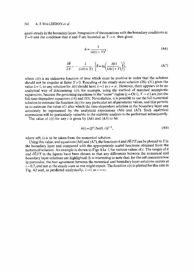
342 A.J. HILLESDON et al.
quasi-steady in the boundary layer. Integration of the equations with the boundary conditions at Y=O and the condition that r~ and 0 are bounded as Y~oo then gives:
1 = _ _ _ (A6) (2(0 + 11)2,
OY- (2(t)+ Y) ~ \(2(t)+ Y)]J '
where 2(t) is an unknown function of time which must be positive in order that the solution should not be singular at finite Y>0. Rescaling of the steady state solution (28)-(31) gives the value 2 - 1 , so any solution for 2(t) should have 2 ~ 1 as t ~ oo. However, there appears to be no analytical way of determining 2(t), for example, using the method of matched asymptotic expansions, because the governing equations in the "outer" region (z = O(1), Y~ oo) are just the full time-dependent equations (14) and (15). Nevertheless, it is possible to use the full numerical solution to estimate the function 2(t) for any particular set of parameter values, and this permits us to estimate the value of t after which the time-dependent solution in the boundary layer can accurately be represented by the analytical expressions (A6) and (AT). Such analytical expressions will be particularly valuable in the stability analysis to be performed subsequently.
The value of 2(0 for any t is given by (A6) and (A3) to be:
2(t) = (fl:/An(O, t)) ~/2, (A8)
where n(0, t) is to be taken from the numerical solution. Using this value, and equations (A6) and (A7), the functions fi and ~0/~ Ycan be plotted vs Yin
the boundary layer and compared with the appropriately scaled functions obtained from the numerical solution. An example is shown in Figs Ala-f, for various values of t. The ranges of and ~0/~ Y in the figures have been chosen so that any differences between the numerical and boundary layer solutions are highlighted. It is interesting to note that, for the cell concentration in particular, the best agreement between the numerical and boundary layer solutions occurs at t = 0.7, and not at the steady state as one might expect. The function 2(Q is plotted for this case in Fig. A2 and, as predicted analytically, 2 ~ 1 as t ~ oo.
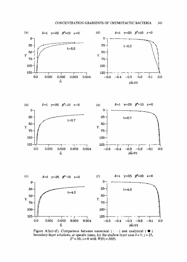
CONCENTRATION GRADIENTS OF CHEMOTACTIC BACTERIA 343
(a)
0-
25-
y 5 0 - I 75-
100-
125 t 0.0
6=1 7=25 #~--10 e:O (d)
0 -
25-
5 0 - Y
75 -
100-
I 125 0.001 0.002 0.003 0.004
fi
6=1 7=25 #2=10 ~=0
t=0.2
1 1 I
-0.5 -0 .4 -0.3 -0.2 -0.1 0.0
aOlaY
(b) 0-
25-
50- Y
75-
100-
125 0.0
5=1 7=25 ,88=10 e=O
f t=0.7
I i I I
0.001 0.002 0.003 0.004 fi
(e)
0-
25-
50- Y
75-
100-
125
5=1 7=25 #z=lO e=O
t=0.7
-0 .5 -0 .4 -0.3 -0 .2 -0.1 0.0 a~/oY
(e)
0 -
6=1 7=25 lSa=lO e=O
50- Y
75-
100-
1 2 5 j
t=4.0
0.0 1 I I
0.001 0.002 0.003 0.004 fi
(f)
0 -
25-
50- Y
75-
1 0 0 -
125-
6=1 7=25 #~=10 e=0
t=4.0
I l I -0 .5 -0 .4 -0 .3 -0.2 -0.1 0.0
o~/oY
Figure Al(a)-(f). Comparison between numerical ( - - ) and analytical ( -0- ) boundary-layer solutions, at specific times, for the shallow-layer case 6 = 1, 7 = 25,
f12= 10, e = 0 with W(O)=H(O).
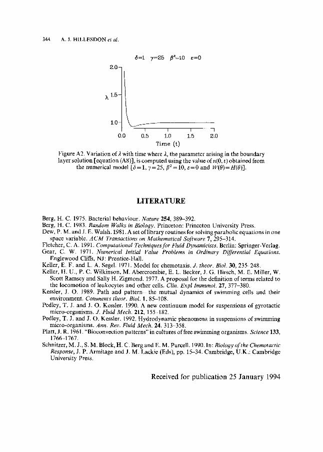
344 A.J. HILLESDON et al.
5=1
2.0-
x l ' 5 -
1.0-
?,=25 fl~=lO ~=0
I I I I
0.0 0.5 1.0 1.5 2.0 Time (t)
Figure A2. Variation of 2 with time where 2, the parameter arising in the boundary layer solution [equation (A8)], is computed using the value of n(O, t) obtained from
the numerical model [6= 1, 7=25, f12= 10, e=0 and W(O)=H(O)].
L I T E R A T U R E
Berg, H. C. 1975. Bacterial behaviour. Nature 254, 389-392. Berg, H. C. 1983. Random Walks in Biology. Princeton: Princeton University Press. Dew, P. M. and J. E. Walsh. 1981. A set of library routines for solving parabolic equations in one
space variable. A CM Transactions on Mathematical Software 7, 295-314. Fletcher, C. A. 1991. Computational Techniques for Fluid Dynamicists. Berlin: Springer-Verlag. Gear, C. W. 1971. Numerical Initial Value Problems in Ordinary Differential Equations.
Englewood Cliffs, NJ: Prentice-Hall. Keller, E. F. and L. A. Segel. 1971. Model for chemotaxis. J. theor. Biol. 30, 235-248. Keller, H. U., P. C. Wilkinson, M. Abercrombie, E. L. Becker, J. G. Hirsch, M. E. Miller, W.
Scott Ramsey and Sally H. Zigmond. 1977. A proposal for the definition of terms related to the locomotion of leukocytes and other cells. Clin. Expl Immunol. 27, 377-380.
Kessler, J. O. 1989. Path and pattern--the mutual dynamics of swimming cells and their environment. Comments theor. Biol. 1, 85-108.
Pedley, T. J. and J. O. Kessler. 1990. A new continuum model for suspensions of gyrotactic micro-organisms. J. Fluid Mech. 212, 155-182.
Pedley, T. J. and J. O. Kessler. 1992. Hydrodynamic phenomena in suspensions of swimming micro-organisms. Ann. Rev. Fluid Mech. 24, 313-358.
Platt, J. R. 1961. "Bioconvection patterns" in cultures of free swimming organisms. Science 133, 1766-1767.
Schnitzer, M. J., S. M. Block, H. C. Berg and E. M. Purcell. 1990. In: Biology of the Chemotactic Response, J. P. Armitage and J. M. Lackie (Eds), pp. 15-34. Cambridge, U.K.: Cambridge University Press.
Received for pub l i ca t ion 25 J a n u a r y 1994